finite state machine watermarking scheme using genetic ... · finite state machine watermarking...
TRANSCRIPT
Finite State Machine Watermarking
Scheme using Genetic Algorithms for
IP Cores Protection
by
Jorge Echavarria
A Dissertation Submitted to the Program in Computer Science.
Computer Science Department in partial fulfillment of the
requirements for the degree of
MASTER IN COMPUTER SCIENCE
at the
National Institute for Astrophysics, Optics and Electronics
November, 2014
Tonantzintla, Puebla
Advisores:
Alicia Morales · Rene Cumplido
Computer Science Department
INAOE
c©INAOE 2014
The author hereby grants to INAOE
permission to reproduce and to distribute copies
of this thesis document in whole part.

To Dalia
Contents
Acronyms xi
Acknowledgements xii
Abstract xiii
Resumen xiv
1 Introduction 1
1.1 Motivation . . . . . . . . . . . . . . . . . . . . . . . . . . . . . . . . . 2
1.2 Goals . . . . . . . . . . . . . . . . . . . . . . . . . . . . . . . . . . . . 3
1.3 Methodology . . . . . . . . . . . . . . . . . . . . . . . . . . . . . . . 3
1.4 Contribution to knowledge . . . . . . . . . . . . . . . . . . . . . . . . 5
1.5 Thesis organization . . . . . . . . . . . . . . . . . . . . . . . . . . . . 5
2 Literature review 7
2.1 Basic concepts . . . . . . . . . . . . . . . . . . . . . . . . . . . . . . . 7
2.1.1 Finite state machine basis . . . . . . . . . . . . . . . . . . . . 7
iii
2.1.2 Watermarking concepts . . . . . . . . . . . . . . . . . . . . . . 9
2.1.3 Evolutionary algorithms . . . . . . . . . . . . . . . . . . . . . 12
2.2 State-of-the-art . . . . . . . . . . . . . . . . . . . . . . . . . . . . . . 14
2.2.1 IP core protection . . . . . . . . . . . . . . . . . . . . . . . . . 14
2.2.2 FSM extraction . . . . . . . . . . . . . . . . . . . . . . . . . . 16
2.2.3 FSM reduction . . . . . . . . . . . . . . . . . . . . . . . . . . 17
3 FSM watermarking procedure 20
3.1 Proposed FSM extraction . . . . . . . . . . . . . . . . . . . . . . . . 22
3.2 Proposed watermark translation . . . . . . . . . . . . . . . . . . . . . 25
3.3 FSM merging . . . . . . . . . . . . . . . . . . . . . . . . . . . . . . . 29
3.3.1 Combinatorial merging . . . . . . . . . . . . . . . . . . . . . . 29
3.3.2 GA based merging . . . . . . . . . . . . . . . . . . . . . . . . 32
3.4 Watermarked FSM reduction . . . . . . . . . . . . . . . . . . . . . . 37
3.4.1 Combinatorial reduction . . . . . . . . . . . . . . . . . . . . . 38
3.4.2 GA based reduction . . . . . . . . . . . . . . . . . . . . . . . . 43
3.5 Selecting the best watermarked design . . . . . . . . . . . . . . . . . 51
3.6 Transitions regrouping . . . . . . . . . . . . . . . . . . . . . . . . . . 53
3.7 Validation . . . . . . . . . . . . . . . . . . . . . . . . . . . . . . . . . 56
3.7.1 Original functionality . . . . . . . . . . . . . . . . . . . . . . . 56
3.7.2 Signature . . . . . . . . . . . . . . . . . . . . . . . . . . . . . 59
4 Experimental results analysis 60
4.1 Experimental setup . . . . . . . . . . . . . . . . . . . . . . . . . . . . 60
4.1.1 Random seeds . . . . . . . . . . . . . . . . . . . . . . . . . . . 61
4.1.2 GA specifics for merging . . . . . . . . . . . . . . . . . . . . . 61
4.1.3 GA specifics for reduction . . . . . . . . . . . . . . . . . . . . 62
4.2 Reported results . . . . . . . . . . . . . . . . . . . . . . . . . . . . . . 62
4.3 Statistical analysis . . . . . . . . . . . . . . . . . . . . . . . . . . . . 65
4.3.1 Wilcoxon signed-rank test . . . . . . . . . . . . . . . . . . . . 66
5 Conclusions 70
5.1 Remarks . . . . . . . . . . . . . . . . . . . . . . . . . . . . . . . . . . 70
5.2 Future work . . . . . . . . . . . . . . . . . . . . . . . . . . . . . . . . 71
5.3 Contributions . . . . . . . . . . . . . . . . . . . . . . . . . . . . . . . 71
Appendices 73
A Wilcoxon signed-rank test 74
B List of equations 78
C VHDL encoding 82

List of Figures
2.1 Hanging states example . . . . . . . . . . . . . . . . . . . . . . . . . 10
3.1 Watermarking Stages flow chart . . . . . . . . . . . . . . . . . . . . . 21
3.2 Loop patterns . . . . . . . . . . . . . . . . . . . . . . . . . . . . . . . 25
3.3 Loop patterns and FSM recognition . . . . . . . . . . . . . . . . . . . 26
3.4 FSMs to be merged . . . . . . . . . . . . . . . . . . . . . . . . . . . . 28
3.5 Don’t care minimization . . . . . . . . . . . . . . . . . . . . . . . . . 31
3.6 Combinatorial FSM merging . . . . . . . . . . . . . . . . . . . . . . . 32
3.7 Merging example . . . . . . . . . . . . . . . . . . . . . . . . . . . . . 35
3.8 Crossover example at position 6. . . . . . . . . . . . . . . . . . . . . . 36
3.9 Mutation example at position 2. . . . . . . . . . . . . . . . . . . . . . 36
3.10 Genetic FSM Merging . . . . . . . . . . . . . . . . . . . . . . . . . . 37
3.11 FSM to be minimized . . . . . . . . . . . . . . . . . . . . . . . . . . . 38
3.12 Combinatorial FSM Reduction . . . . . . . . . . . . . . . . . . . . . . 43
3.13 Crossover example at position 3 . . . . . . . . . . . . . . . . . . . . . 45
vi
3.14 Mutation example at position 2. . . . . . . . . . . . . . . . . . . . . . 46
3.15 Cloud points from different configurations. . . . . . . . . . . . . . . . 48
3.16 Plane interpolation from the cloud points. . . . . . . . . . . . . . . . 50
3.17 Genetic FSM Reduction . . . . . . . . . . . . . . . . . . . . . . . . . 51
3.18 Asymptotes behavior . . . . . . . . . . . . . . . . . . . . . . . . . . . 53
3.19 FSM before and after Don’t Care Minimization . . . . . . . . . . . . 54
3.20 Don’t care minimization of Figure 3.12 . . . . . . . . . . . . . . . . . 56
3.21 FSMs to validate . . . . . . . . . . . . . . . . . . . . . . . . . . . . . 57
3.22 FSMs merging . . . . . . . . . . . . . . . . . . . . . . . . . . . . . . . 59
4.1 z value location in Normal Distribution and its p-value. . . . . . . . . 68
A.1 Distributions of nr . . . . . . . . . . . . . . . . . . . . . . . . . . . . 76
B.1 Sum of all equations. . . . . . . . . . . . . . . . . . . . . . . . . . . . 81
C.1 Next State example . . . . . . . . . . . . . . . . . . . . . . . . . . . . 85
List of Tables
3.1 Probabilities of inserting all the packages. . . . . . . . . . . . . . . . 28
3.2 Transitions to obtain satisfying chain from Figure 3.4b . . . . . . . . 29
3.3 Next-State flow table . . . . . . . . . . . . . . . . . . . . . . . . . . . 40
3.4 Output flow table . . . . . . . . . . . . . . . . . . . . . . . . . . . . . 40
3.5 Compatibilities from Flow Tables 3.3 and 3.4 after 1 iteration . . . . 41
3.6 Compatibilities from Flow Tables 3.3 and 3.4 after a second iteration 42
3.7 Compatibility classes from table 3.6 after second iteration. . . . . . . 42
3.8 φ(x, y) behavior . . . . . . . . . . . . . . . . . . . . . . . . . . . . . . 54
3.9 Transitions regrouping . . . . . . . . . . . . . . . . . . . . . . . . . . 55
3.10 Don’t care minimization steps . . . . . . . . . . . . . . . . . . . . . . 55
3.11 Flow tables . . . . . . . . . . . . . . . . . . . . . . . . . . . . . . . . 58
3.12 Compatibilities of Flow Tables 3.11a and 3.11b . . . . . . . . . . . . . 58
4.1 Comparative table of number of final transitions from Cui’s method
inserting 128 bits [15], and the proposed method inserting 160 bits of
FMS’s. . . . . . . . . . . . . . . . . . . . . . . . . . . . . . . . . . . . 63
viii

4.2 Number of final states from Adbel’s method inserting 40 bits [2], and
the proposed method inserting 160 bits. . . . . . . . . . . . . . . . . . 64
4.3 Number of final hanging states. . . . . . . . . . . . . . . . . . . . . . 65
4.4 Sampling Population with watermark . . . . . . . . . . . . . . . . . . 67
4.5 Sampling Population without watermark . . . . . . . . . . . . . . . . 69
A.1 Possible differences from 3 ranks . . . . . . . . . . . . . . . . . . . . . 76
List of Algorithms
1 GAs general structure. . . . . . . . . . . . . . . . . . . . . . . . . . . . 13
2 Finding and labeling nodes. . . . . . . . . . . . . . . . . . . . . . . . . 23
3 Modules labeling. . . . . . . . . . . . . . . . . . . . . . . . . . . . . . . 24
4 Loops recognition and FSM extraction. . . . . . . . . . . . . . . . . . 24
5 Translating a watermark into a FSM. . . . . . . . . . . . . . . . . . . . 27
6 Combinatorial FSM merging. . . . . . . . . . . . . . . . . . . . . . . . 30
7 GA based FSM merging. . . . . . . . . . . . . . . . . . . . . . . . . . . 33
8 Genetics from GA based FSM merging. . . . . . . . . . . . . . . . . . 34
9 Combinatorial FSM reduction. . . . . . . . . . . . . . . . . . . . . . . 39
10 GA based FSM reduction. . . . . . . . . . . . . . . . . . . . . . . . . . 43
11 Genetics from GA based FSM reduction. . . . . . . . . . . . . . . . . . 44
x
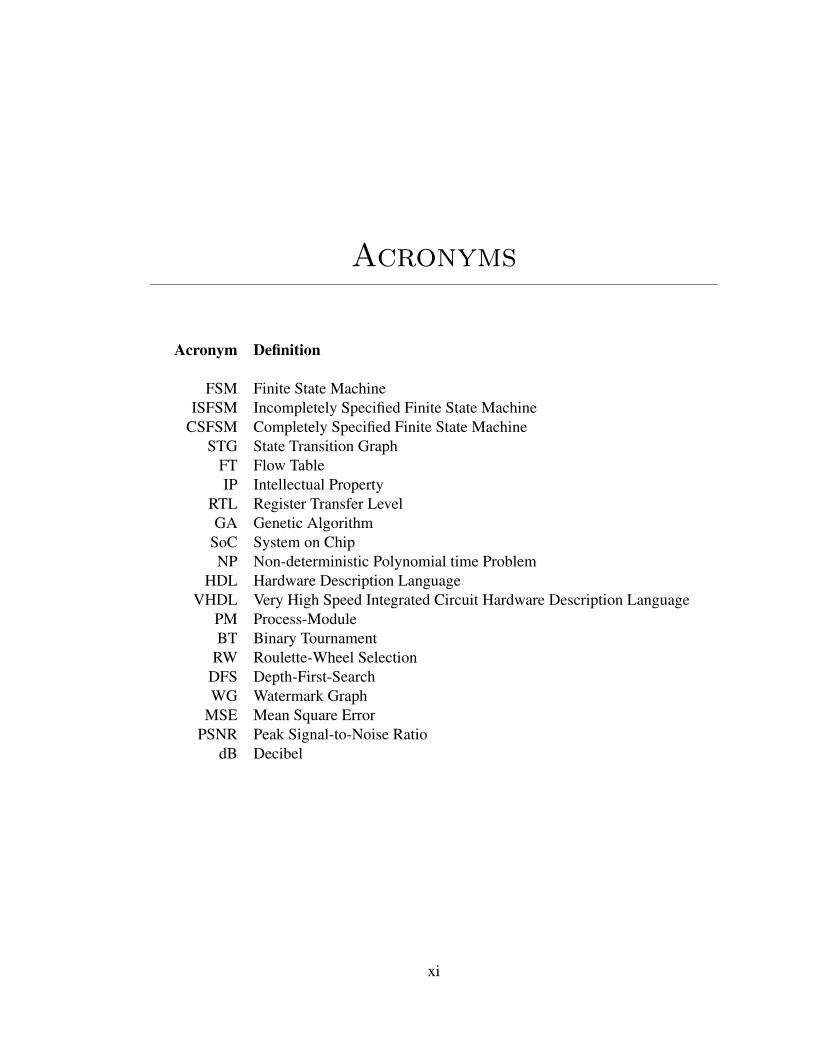
Acronyms
Acronym Definition
FSM Finite State MachineISFSM Incompletely Specified Finite State Machine
CSFSM Completely Specified Finite State MachineSTG State Transition Graph
FT Flow TableIP Intellectual Property
RTL Register Transfer LevelGA Genetic Algorithm
SoC System on ChipNP Non-deterministic Polynomial time Problem
HDL Hardware Description LanguageVHDL Very High Speed Integrated Circuit Hardware Description Language
PM Process-ModuleBT Binary Tournament
RW Roulette-Wheel SelectionDFS Depth-First-SearchWG Watermark Graph
MSE Mean Square ErrorPSNR Peak Signal-to-Noise Ratio
dB Decibel
xi

Acknowledgements
I want to thank to Dr. Morales and Dr. Cumplido for all their support and advice.
Whenever I needed their counsel, whether or not related to my thesis, they were
there for me.
Thank you for your dedication and generosity and your boundless patience and en-
couragement. My most sincere gratitude to both of you.
I thank my mother for everything she has done for me. I would not have accom-
plished absolutely anything without her. And I thank my father for all his support
and, well, just for being him.
Thank you Dalia for always supporting me, you are my inspiration.
Esta investigacion fue realizada con el apoyo del Consejo Nacional de Ciencia y
Tecnologıa (CONACyT) y el Consejo de Ciencia y Tecnologıa del Estado de Puebla
(CONCyTEP)
xii
Abstract
This thesis proposes an improved procedure to watermark Intellectual Property
Cores at Register Transfer Level using Genetic Algorithms. First, watermarking
signature and Intellectual Property Core’s behavioral description are translated into
Finite State Machines in preparation for merging. The resulting Finite State Ma-
chine contains the watermarked Intellectual Property Core maintaining its original
functionality without disruption. Next, a reduction procedure is applied to the wa-
termarked design. At this stage, dealing with hanging states is challenging, if any
of these is deleted, the watermark could be removed and possibly the original In-
tellectual Property Core functionality would not be disrupted. Both Finite State
Machine merging and reduction are NP-Complete problems. In this study an im-
proved objective function is proposed to accurately model the Finite State Machine
reduction problem while applying Genetic Algorithms as optimization techniques at
both stages. Empirical results show a significant improvement in terms of the num-
ber of final hanging states and watermark embedding strength as regards previous
reported approaches.
Results of applying the proposed technique to watermark a number of Finite
State Machines are presented and discussed.
xiii
Resumen
Esta tesis propone un procedimiento para insertar marcas de agua en IP Cores a
nivel de transferencia de registros usando Algoritmos Geneticos. Primero, la firma
y la descripcion del comportamiento del IP Core son traducidos a maquinas de es-
tados finitos para despues ser fusionadas. La maquina de estados finitos resultante
contendra el IP Core firmado manteniendo la funcionalidad original sin ninguna
alteracion. Despues, es aplicado un procedimiento de reduccion de estados al diseno
firmado. Un reto importante en esta etapa es el de lidiar con estados colgantes, que
son un subconjunto de estados pertenecientes a la maquina de estados de la firma, y
que al eliminar cualquier de estos estados, la marca de agua puede ser eliminada sin
alterarse la funcionalidad original. Ambos problemas de fusion y reduccion, son NP-
completos. En este estudio se ha propuesto una funcion objetivo mejorada para mod-
elar adecuadamente el problema de reduccion aplicando algoritmos geneticos como
tecnicas de optimizacion en ambas etapas.
Resultados empıricos muestran mejoras significativas en terminos del numero
final de estados colgantes y en la fuerza de la firma embebida en comparacion con
enfoques reportados en la literatura.
xiv
Chapter 1
Introduction
Throughout history, watermarking has been widely used for copyright protection.
Existing techniques essentially consist in taking advantage of high information re-
dundancy and susceptibility ranges of human’s eye and ear. Inserting the watermark
out of perception boundaries, allows the human to not discern any variation of the
digital media even after been watermarked [29].
In the area of embedded systems, specially in the last pair of decades, the
use of Systems on Chip (SoC), has impacted profoundly and became widespread
alongside manufacturers. Intellectual Property (IP) Cores, reusable logic units, are
widely used in electronic design. Thus, their authenticity is at risk when licensing
to a second party or during redistribution [54].
There are two types of IP Cores, hard and soft cores. Hard cores are the
physical description of some chip and they are commonly offered in binary represen-
tation [32]. Soft cores, on the other hand, are descriptions at higher levels. They
can be distributed as netlists, representing the logical implementation at gate-level.
These kinds of core give the original developer certain security when distributing
multiple times due to the their high reverse engineering complexity. Soft cores have
an even higher description level. Register Transfer Level (RTL) permits designers to
develop their designs in a Hardware Description Language (HDL), such as VHDL
and Verilog.
1
CHAPTER 1. INTRODUCTION 2
The technique proposed in this study inserts the watermark at synthesizable
RTL by modifying its behavioral description. The proposal extracts and merge
Finite State Machines (FSMs) from the IP Core and the watermark respectively.
To achieve this, it is proposed to merge both FSMs using a Genetic Algorithm (GA).
Media watermarking permits to lose data with little information, nevertheless, circuit
watermarking must contain all of its original data at the end the signature must be
difficult to remove, an issue which is tackled by a FSM reduction also based in GAs.
It is also proposed an improvement when designing objective functions aimed to
state reduction by reducing the space of satisfaction.
Among other advantages, IP Cores watermarking by merging and reducing
involving FSMs leads to enhance heat and power dissipation [55] and an effective
use of chip area by reducing the number of flip-flops and gates needed for imple-
mentation [5], fewer states permit handling a less significant number of don’t cares.
Furthermore, as pointed out by Christoforos, digital sequential systems operating
over several time steps, can lead to a state-transition fault usually handled by merg-
ing the original FSM into a larger one that identifies and corrects errors [14].
1.1 Motivation
IP reuse is becoming more and more common nowadays, however, sharing IP Cores
in this competitive market can lead to copyright issues. Inserting a signature into
the circuit behavior results in a secure way to share this information.
It has been previously proposed by several authors, techniques to watermark
FSMs [2,6,15,34,54], however, it has been observed previous to the FSM merging, a
set of hanging states, a group of states from the signature which are not deeply em-
bedded (Defined in Section 2.1.1). It was noted that if any of these states is deleted,
the watermark vanishes, in some cases without disrupting the original functionality,
allowing to copyright infringements.
CHAPTER 1. INTRODUCTION 3
1.2 Goals
The main goal is to watermark IP Cores by FSMs merging using GAs, achieving
invariance of the original design by not disrupting the primary functionality. The
original functionality must be lost if someone tries to delete any part of the signature.
That is, signature and design must be tightly bound.
The particular objectives are:
• To obtain a merged FSM containing the original functionality within the wa-
termark.
• To analyze critical scenarios which could cause losing the watermark.
• To analyze the proposed objective functions oriented to FSM state-reduction
in the literature to better understand the behavior and propose a better way
to narrow the search space.
• To improve the state-reduction process.
• To conduct a comparative empirical analysis related to deterministic and ge-
netic approaches to merging and reduction processes.
• To define a selection criteria of the most appropriate combination of algorith-
mic techniques that solve specific merging and reduction problems.
1.3 Methodology
Below the methodology of the proposed approach will be explained.
CHAPTER 1. INTRODUCTION 4
FSMs extraction
The first step is to extract the FSM which represents the IP Core behavior, then,
it is translated into a FSM the watermark. Both steps are described in Sections 3.1
and 3.2 respectively.
Embedding procedure
After obtaining both FSMs, they are merged to obtain a single FSM with the signa-
ture embedded. That is, after the embedding procedure, the IP Core FSM will be
already watermarked. Nevertheless, after this merging process, a state-reduction is
performed. In Section 3.3.1 a deterministic merging method is described. In Section
3.3.2 a GA based approach is described.
Objective function
In Section 3.4.2 a GA based state-reduction of the watermarked FSM is presented.
To obtain the objective function, a base function was proposed and the behavior
of different state-reduction functions was analyzed to, based on their behavior, to
define the coefficients of said function.
FSM reductions
There are two different types of FSM reduction. First there is a state-reduction
proceeding which is aimed to fuse all compatible states with two different approaches,
one deterministic described in Section 3.4.1, and a GA based approach, described
in Section 3.4.2. The second type of FSM reduction is oriented to transitions, this
reduction is performed by combining similar transitions by regrouping, this method
is explained in Section 3.6.
CHAPTER 1. INTRODUCTION 5
Selecting the best result
As seen above, deterministic and stochastic approaches to perform different pro-
ceedings are used. Thus, there will be 4 different watermarked FSMs and it will be
necessary to choose the most convenient. In Section 3.5 is presented an equation to
select the best result.
1.4 Contribution to knowledge
Limiting the search space of the objective function that evaluates the possible solu-
tions from the GA focused on state-reduction of FSMs, from fitting the model of a
plane of a set of equations that describe the problem.
Empirical analysis of the use of stochastic techniques, particularly GAs aimed
to optimize FSM merging and state reduction processes.
The presence of hanging nodes is critical during watermarking process. Pre-
vious studies by other authors do not address this issue, and to the best of our
knowledge, it is the first time that hanging states are considered, how these states
would affect the watermarking process and how stochastic techniques such as GAs
deal successfully with them.
1.5 Thesis organization
Chapter 2 reviews previous work and theoretical framework related to the method
presented in this thesis. In Chapter 3 each developed algorithm is described; going
through FSMs extraction, merging, reduction and re-translation to Hardware De-
scription Language (HDL); signal validations and synthesis verification is also pre-
sented. In Chapter 4 statistical justifications and experimental results are presented.

CHAPTER 1. INTRODUCTION 6
Finally, in Chapter 5 the conclusions drawn during this project are presented.
Chapter 2
Literature review
This chapter introduces several concepts related to the proposed watermarking
scheme based on Genetic Algorithms (GA) for Intellectual Property (IP) Core pro-
tection. It also presents an extensive literature review of closely related topics to-
gether with several authors and state of the art research in order to contextualize
this thesis work.
2.1 Basic concepts
In this section, basic terminology required to fully understand the method proposed
in this research is described.
2.1.1 Finite state machine basis
A finite state system can be modeled by one or more Finite State Machines (FSM)
that produce outputs on their transitions after receiving inputs [33].
An FSM M is a quintuple
M = (I, S,O, δ, λ)
where I is a finite set of input symbols, S is a finite set of states and O is a finite
7
CHAPTER 2. LITERATURE REVIEW 8
set of output symbols.
δ : S × I → S is the next state function.
λ : S × I → O is the output function.
When the FSM is in a current state si ∈ S and receives an input ai ∈ I,
it moves to the next state by si+1 = δ(si, ai) with si+1 ∈ S and gives as output
bi = λ(si, ai) with bi ∈ O.
LetM(S,E) be a FSM, where E are the transitions. Each transition e(si, si+1) ∈
E with si and si+1 ∈ S, represents state si is a fanin of state si+1 and state si+1 is
a fanout of state si.
FSMs can be represented as State Transition Graphs (STG) and Flow Tables
(FT). STGs are directed graphs whose vertices and edges correspond to states and
state transitions from the FSM respectively [9]. As the STG of an FSM is a directed
graph, graph theory concepts and algorithms are useful in FSM’s analysis. A FT is
a table with rows representing states and columns representing input symbols; an
intersection of a row with a column corresponds to a next state and an output.
An FSM is a Completely Specified Finite State Machine (CSFSM) if there is
a specified next state by the state transition function and a specified output by the
output function for any state and its input. Otherwise, when there are states with
an input that do not have a specific next state or output, the FSM is an Incompletely
Specified Finite State Machine (ISFSM) [22].
Any pair of states si and sj from S are compatible, if and only if, for every
input sequence the next state and the output of si are the same as sj.
λ(δ(si, a(n+1)), a1...an) = λ(δ(sj, a(n+1)), a1...an) (2.1)
A states set Ci = {si1, si2, ..., sin} is called a compatible class if every pair of states
CHAPTER 2. LITERATURE REVIEW 9
is compatible [48]. Cij is the next states set of Ci for every input ai in I. It is said
that Cij is implied by Ci for every input ai in I. Pi is the set of all compatibles
Cij implied by Ci, such that Ci and Pi are disjoint, that is, the cardinality of Cij is
greater than 1, Cij 6⊂ Ci and Ci 6⊂ Cik if Cik ∈ Pi. A compatible Ci dominates a
compatible Cj if Cj ⊂ Ci and Pi ⊂ Pj. A compatible class which is not dominated
by any other is called compatibility prime class (PC). A set of compatible states
Ci is maximal if it is not a subset of another set of compatible states. A set of
compatibles C = {C1, C2, ..., Cn} is closed if, for each element Ci ∈ C, the implied
Cij∀ai is also an element of C.
Let M = (I, S,O, δ, λ) and M ′ = (I, S ′, O, δ′, λ′) be two FSMs with same input
and output sets. If for every state s in S and for every input a in I, it holds that
δ′(φ(s), a) = φ(δ(s, a)) and λ′(φ(s), a) = λ(s, a) and φ is a bijective mapping from S
to S ′, then M and M ′ are isomorphic, that is, both FSMs have the same number of
states and are identical, except for the name of the states.
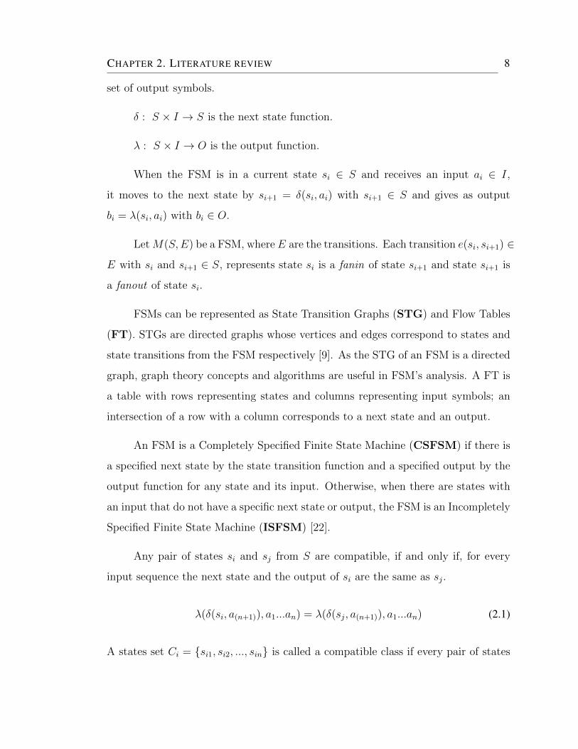
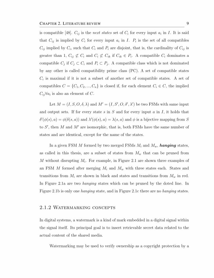
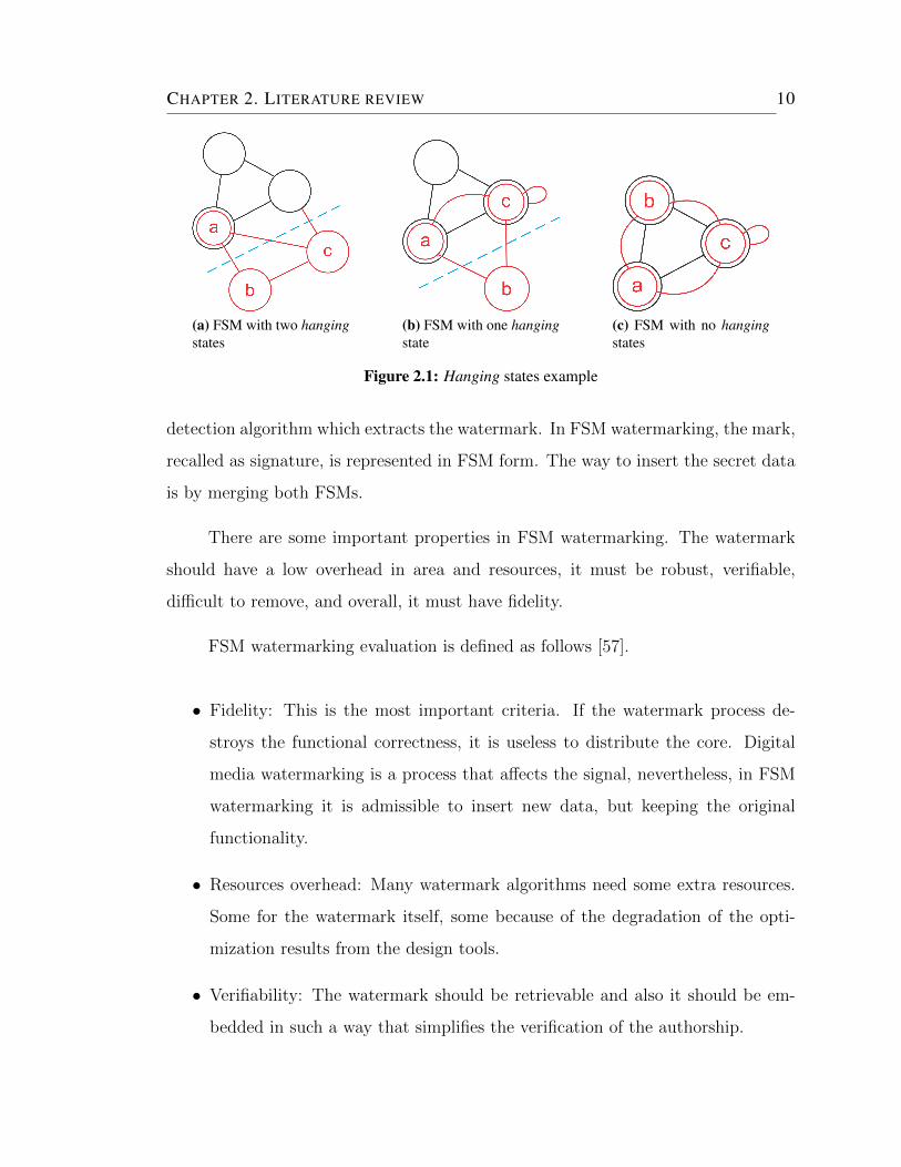
In a given FSM M formed by two merged FSMs Mi and Mw, hanging states,
as called in this thesis, are a subset of states from Mw that can be pruned from
M without disrupting Mi. For example, in Figure 2.1 are shown three examples of
an FSM M formed after merging Mi and Mw with three states each. States and
transitions from Mi are shown in black and states and transitions from Mw in red.
In Figure 2.1a are two hanging states which can be pruned by the doted line. In
Figure 2.1b is only one hanging state, and in Figure 2.1c there are no hanging states.
2.1.2 Watermarking concepts
In digital systems, a watermark is a kind of mark embedded in a digital signal within
the signal itself. Its principal goal is to insert retrievable secret data related to the
actual content of the shared media.
Watermarking may be used to verify ownership as a copyright protection by a
CHAPTER 2. LITERATURE REVIEW 10
(a) FSM with two hangingstates
(b) FSM with one hangingstate
(c) FSM with no hangingstates
Figure 2.1: Hanging states example
detection algorithm which extracts the watermark. In FSM watermarking, the mark,
recalled as signature, is represented in FSM form. The way to insert the secret data
is by merging both FSMs.
There are some important properties in FSM watermarking. The watermark
should have a low overhead in area and resources, it must be robust, verifiable,
difficult to remove, and overall, it must have fidelity.
FSM watermarking evaluation is defined as follows [57].
• Fidelity: This is the most important criteria. If the watermark process de-
stroys the functional correctness, it is useless to distribute the core. Digital
media watermarking is a process that affects the signal, nevertheless, in FSM
watermarking it is admissible to insert new data, but keeping the original
functionality.
• Resources overhead: Many watermark algorithms need some extra resources.
Some for the watermark itself, some because of the degradation of the opti-
mization results from the design tools.
• Verifiability: The watermark should be retrievable and also it should be em-
bedded in such a way that simplifies the verification of the authorship.
CHAPTER 2. LITERATURE REVIEW 11
• Difficult to remove: The watermark should be resistant against removal attack.
The effort to remove the watermark should be greater than an effort needed to
develop a new core or removal of watermark should cause corruptness of the
functionality of the core. Watermarks which are embedded into the function
of the core are more robust against removal than additive watermarks.
• Strong proof of authorship: The watermark should identify the author with
a strong proof. It should be impossible that other persons can claim the
ownership of the core.
• Robust: Meaning that even after adding new transitions or states, the sig-
nature should remain. The watermark procedure must be resistant against
tampering.
In his work, Kalker provided the following watermarking definitions [27]:
- “Robust watermarking is a mechanism to create a communication channel that
is multiplexed into original content”, and which capacity “degrades as a smooth
function of the degradation of the marked content”.
- “Security refers to the inability by unauthorized users to have access to the raw
watermarking channel”. Such an access refers to trying to “remove, detect and
estimate, write and modify the raw watermarking bits”.
There are three types of attacks against FSM watermarking [39].
• Removal attack: Removal attacks are aimed to completely or partially remove
the signature from the watermarked FSM. There are two kinds of removal
attacks. The watermarked FSM can either have states deleted, or they can be
masked in such a way that the signature is no longer retrievable. These types
of attack do not need to know the input signal needed to obtain the signature
back.
CHAPTER 2. LITERATURE REVIEW 12
• Embedding attack: Embedding attacks are aimed to reinsert a signature into
the watermarked design. This is possible by searching a new sequence of states
that will be considered as the new watermark, or by embedding a completely
new signature.
• Read-back Attack: Read-back is a feature that is provided for most FPGA
families. This feature allows to read a configuration out of the FPGA for
easy debugging. The idea of the attack is to read the configuration of the
FPGA through the JTAG or programming interface in order to obtain secret
information.
2.1.3 Evolutionary algorithms
Evolutionary Algorithms (EA) are described in [40] as follows.
- “EAs are non-deterministic techniques that follow the Darwinian Principle of Evo-
lution. A population is randomly or under certain conditions created and formed
by individuals. Competition for survival among individuals determines which ones
will reproduce and pass their genetic material to new individuals in following gen-
erations”.
GAs are a subclass and the most known type of EAs [19]. A GA is a search
heuristic inspired in the process of biologic evolution and natural selection and their
molecular-genetic base. GAs do not guarantee to find the optimal solution of a
certain problem as any other deterministic algorithm, if there is an algorithm to solve
said problem. However, GAs do not attempt to enumerate all possible solutions of
the problem. On the contrary, these heuristic algorithms have the ability to decide
which solutions should survive the evolution process, based on “how close” they are
from the best solution [17]. In Algorithm 1 is presented the general structure of a
GA [19].
CHAPTER 2. LITERATURE REVIEW 13
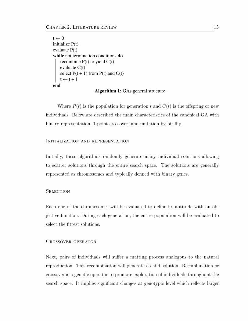
t← 0initialize P(t)evaluate P(t)while not termination conditions do
recombine P(t) to yield C(t)evaluate C(t)select P(t + 1) from P(t) and C(t)t← t + 1
endAlgorithm 1: GAs general structure.
Where P (t) is the population for generation t and C(t) is the offspring or new
individuals. Below are described the main characteristics of the canonical GA with
binary representation, 1-point crossover, and mutation by bit flip.
Initialization and representation
Initially, these algorithms randomly generate many individual solutions allowing
to scatter solutions through the entire search space. The solutions are generally
represented as chromosomes and typically defined with binary genes.
Selection
Each one of the chromosomes will be evaluated to define its aptitude with an ob-
jective function. During each generation, the entire population will be evaluated to
select the fittest solutions.
Crossover operator
Next, pairs of individuals will suffer a matting process analogous to the natural
reproduction. This recombination will generate a child solution. Recombination or
crossover is a genetic operator to promote exploration of individuals throughout the
search space. It implies significant changes at genotypic level which reflects larger

CHAPTER 2. LITERATURE REVIEW 14
steps for exploring new solutions.
Mutation operator
The offspring is later mutated to maintain genetic diversity or to be able to avoid
convergence to local optima [40]. Mutation is a fine genetic operation which implies
small probability based changes at the genotypic level which would reflect short steps
for solutions moving throughout the search space.
Fitness function
Once applied the genetic operators, there will be selected the best individuals to con-
form the next generation population with the objective function mentioned above.
2.2 State-of-the-art
This section provides a literature review concerning to IP Core watermarking. First,
works related to IP Core protection and the different techniques developed during
the years to signature embedding will be listed and commented. Then, different
approaches to extract FSMs directly form IP Cores description will be enumerated.
And finally, two different techniques to state-reduce FSMs, one deterministic and
one stochastic, are described.
2.2.1 IP core protection
Several authors have proposed different approaches to merge FSMs or to embed
signatures into IP Cores [2, 34], being the first one the proposal of Torunoglu and
Charbon [52]. In a low level description, some authors have inserted the signature
by controlling temperature radiation, electromagnetic radiation, power consumption
CHAPTER 2. LITERATURE REVIEW 15
[56] or after synthesis by flip-flops rearranging [41]. At a higher level, there have
been some other authors that insert the signature by merging internal FSMs or
directing the configuration bit-file by fusing look-up tables, [26, 31]. Nevertheless,
these methods are either slow or very difficult to implement. For example, monitoring
power consumption to read out the signature takes several minutes, and monitoring
radiation is not viable because new metal packages absorb radiation [57].
Some other authors have proposed to merge one or more FSMs found in VHDL
coding at a Register Transfer Level (RTL) with a new FSM representing the water-
mark [2, 6, 15, 16, 34, 54]. Cui proposed a hybrid watermarking technique to double
protect the design at two different abstraction levels, by inserting the watermark
during the FSM design, it makes it more difficult to erase the watermark, and by in-
serting the watermark once the design is integrated into the System on Chip (SoC)
the signature can be more easily identified [15, 16]. In Arunkumar approach, the
signature bits are inserted into the outputs of the existing and free transitions of the
STG obtaining a high tampering resistance, nevertheless, by not adding new transi-
tions the approach can not be practical when dealing with CSFSMs [6]. Abdel et al.
proposed the first public-key scheme, their approach utilizes coinciding and unused
transitions to insert time-stamped authenticated watermark bits [2]. Lewandowski
et al. proposed a greedy heuristic to solve the isomorphism problem when trying to
match the IP FSM and the signature FSM, their justification is the high complexity
when trying reverse engineering to retrieve and or delete the signature [34]. Xu pro-
posed to insert the watermark bits into unused transitions when dealing with ISFSMs
and later to convert this final FSM into a CSFSM; when dealing with CSFSMs, they
proposed to insert all watermark bits into new transitions [54], nevertheless, this can
lead to states than complain with the term of hanging states described in Section
2.1.1.
Although IP Core watermarking by FSMs merging can be translated as a sub-
graph matching problem [28], this novel method provides advantages when monitor-

CHAPTER 2. LITERATURE REVIEW 16
ing SoC signals in real time.
Considering the above, in this work the signature is embedded by using FSMs
merging. To make this possible, it is necessary to extract and latter to merge FSMs
directly related to the behavioral description and the watermark. In the next sub-
section works related to FSM extraction will be commented.
2.2.2 FSM extraction
As described below, there have been several proposals to extract FSMs from VHDL
coding at RTL. Some of them are focused in the coding structure, other ones in
sentences and some others create their own models in a random fashion.
Liu proposed a method for extracting FSMs in Hardware Description Language
(HDL) written at RTL by recognizing FSMs general patterns within the Process-
Module (PM) graph [37] . These general patterns are derived from a relationship
between FSM’s current and next states, not the coding order. Thereby, neither hints
nor comments are needed to recognize FSMs. Kubek proposed to define the central
structure of the Finite State Control as a signal (or more signals) [30]. States are
defined as a set of possible values of those signals. Transitions between states can
be encoded by conditional statements like if and case. Pruteanu presented a tool
capable to generate completely or incompletely FSMs, based on the list of arguments
regarding the number of internal states, and the number of inputs and outputs [46].
Jnagal created POWDER, a program that generates random FSMs [24].
Based in literature review, it has been concluded that the best approach to
extract an FSM from HDL coding, is to insert the signals into the FSM transitions.
This will benefit the final number of states due to data will be contained not in
states, but in transitions, letting to handle in a better way the number of hanging
states, which according to the experimental analysis in this thesis, are considered to
be the most vulnerable component of the watermarked FSMs.
CHAPTER 2. LITERATURE REVIEW 17
2.2.3 FSM reduction
FSMs model different structures functionality like circuits, networks, digital systems,
control units, microprocessors and protocols. In digital systems, the outlining is
generally represented in HDL coding and embedded into digital controllers which
are later synthesized.
The use of these systems is so common nowadays that modern synthesizers
extract FSMs from these codes to reduce them during the synthesis process, de-
creasing the use of silicon, among other advantages. The challenge in this research
is facing the lose of states representing the signature embedded in the FSM when it
is optimized by the synthesizer. Because of that, it is proposed to perform a post
state-reduction of the watermarked FSM.
In state-based minimization, several authors have proposed techniques that
require the enumeration of compatible sets trying to reach some maximal class with
the minimum cardinality. Proposals from deterministic and GA based approaches
are listed and discussed below.
Combinatorial scheme
Because the signature’s embedding is carried out by inserting new transitions, when
the IP Core represents an ISFSM; and new transitions, new states and a control
bit when it represents a CSFSM; redundant data which could be lost during the
synthesizer optimization is inserted. The watermarked FSM will have the original
functionality for any input signal, as long as the control bit had been set.
Combinatorial reduction consists in finding compatible states sets. This set of
compatibles can be recombined in different configurations. The main goal consists
in finding the prime compatibility class with minimum cardinality which covers the
original functionality, therefore, the states set that solves the original problem, the
CHAPTER 2. LITERATURE REVIEW 18
merged FSM in its minimal expression [48].
Since the 50’s, Paull and Unger developed the general theory for ISFSMs and
proposed a tabular technique to find compatibility classes of internal states from a
FSM [42]. Nevertheless, their approach considers a large number of cases.
Later in the 60’s, Grasselli and Lucio showed that only some compatibility
classes need to be considered as members of a solution introducing the concept of
prime classes which assures a minimal solution, and reducing this way the solution
space size [21], a concept that gained certain strength among other authors [47].
Some authors like Avedillo et al. suggested the use of a set of maximal compat-
ibles as the input set [8], nevertheless, it is not guaranteed that only using maximal
compatibles there would be found a minimum closed cover class.
Several approaches, including the ones listed above, start with the strategy of
satisfying the cover condition and then handle the closure condition (refer to Section
2.1.1 for details). Ahmad et al. proposed the idea of switching the order between the
two conditions [5], they presented an algorithm that starts with the closure condition
and then handle the cover condition.
Pena proposed an exact algorithm that is not based on the enumeration of
compatible sets, and, therefore, its performance is not dependent on the number of
prime compatibles [43].
State-minimization implies the resolution of an NP Problem [48]. In [13,18,48]
the efficiency a GA performing a stochastic search to solve the conditions mentioned
above was shown.
CHAPTER 2. LITERATURE REVIEW 19
Genetic scheme
Reduction of the number of states in ISFSMs implies solving a NP-Problem [5, 48].
Thus, some authors suggested GAs to solve this kind of problem [13, 48, 55]. In
Sanchez proposal it is required to find all the elements of some compatibility class,
and with it to generate a minimum closed cover class, including all the states of the
original FSM, this class is called prime compatibility (see Section 2.1.1 for details)
[48]. Sanchez proposed to use GAs due to the high complexity of finding the prime
compatibility, this step is a combinatorial problem classified as NP hard [48]. In his
approach, solutions represent compatibility classes.
Due to their evolutionary nature, GAs will search for solutions regard to the
specific inner workings of the problem; specifically when solving combinatorial prob-
lems, GAs provide a great flexibility and do not require much problem-specific knowl-
edge in order to get good solutions. Besides, these algorithms do not have much
mathematical requirements about the optimization of combinatorial problems [19].
Yinshui et al. presented a GA for FSM encoding to minimize area and power
dissipation [55]. In their work, chromosomes represent states sets as a string of
decimals. Later, Chattopadhyay et al. used binary depiction [13]. Their approach
reduces the number of nodes in the binary decision diagram representation of the
FSM by using a GA based method for area and power minimization.
In the following chapter the proposed FSM watermarking scheme will be pre-
sented. Next, the evaluations will be analyzed. And finally, in Chapter 5, the
conclusions will be discussed.
Chapter 3
FSM watermarking procedure
This chapter presents in an ordered manner the main stages of the proposed water-
marking scheme and in particular, the evolutionary approaches proposed for Finite
State Machine (FSM) merging and reduction stages.
In this thesis, a watermark is embedded within the circuits behavioral de-
scription, to secure ownership at a circuit level by using Combinatorial and Genetic
Algorithms (GAs) to extract, merge and optimize FSMs representing the original
behavior and the watermark.
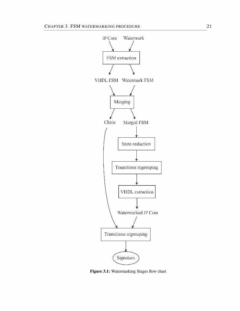
The extraction of the original FSM is explained in Section 3.1, the translation
of the signature FSM is explained in Section 3.2. Those FSMs are merged using
two different approaches. The first approach is a combinatorial algorithm which
operates in a greedy fashion [34] (see Section 3.3.1), the second one, is a GA that
finds the most promising solutions, finding a solution in polynomial time [48] (see
Section 3.3.2).
To secure signature’s states remaining after synthesis, the merged FSM is state-
reduce. The best solution must be selected after reduction, i.e., the solution with
less hanging states remains to next stages.
The reduction also has a combinatorial approach which is explained in Section
3.4.1, and a GA based approach explained in Section 3.4.2.
20
CHAPTER 3. FSM WATERMARKING PROCEDURE 21
Figure 3.1: Watermarking Stages flow chart
CHAPTER 3. FSM WATERMARKING PROCEDURE 22
It is necessary to properly combine adequate algorithms techniques in order to
achieve the best possible solution (see Section 3.5); therefore, the next combinations
are experimentally assessed:
a) Combinatorial Merging & Combinatorial Reduction
b) Combinatorial Merging & GA Based Reduction
c) GA Based Merging & Combinatorial Reduction
d) GA Based Merging & GA Based Reduction
The above procedure’s combinations are investigated in order to determine
which one provides the best performance in terms of copyright protection and FSM
reduction.
All comparisons and experiments were made using FSMs from ACM/SIGDA
benchmarks library [11], specially LGSynth series (High-Level Synthesis Work-
shops) from Collaborative Benchmarking and Experimental Algorithmics Labora-
tory granted by the Design, Verification and Test Division of Mentor Graphics Cor-
poration. It was decided to use this benchmark due to its common use in literature.
3.1 Proposed FSM extraction
Intellectual Property (IP) Cores are regularly offered as synthesizable Hardware
Description Language (HDL) at Register Transfer Level (RTL), typically in VHDL
or Verilog, the dominant HDLs in the electronics industry. In this thesis, VHDL
encoded IP Cores are used for the watermarking process.
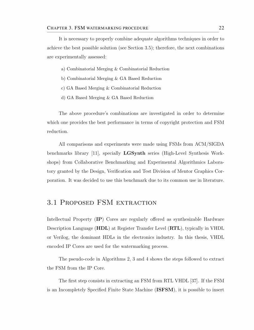
The pseudo-code in Algorithms 2, 3 and 4 shows the steps followed to extract
the FSM from the IP Core.
The first step consists in extracting an FSM from RTL VHDL [37]. If the FSM
is an Incompletely Specified Finite State Machine (ISFSM), it is possible to insert
CHAPTER 3. FSM WATERMARKING PROCEDURE 23
Input: ArchitectureOutput: GraphList of processes← FindProcesses(Architecture)foreach process in List of processes do
if process is triggered by a clock signal thenprocess = Label as SEQ P
elseprocess = Label as COM P
endendforeach a in List of processes do
Graph← InsertNode(node a)foreach b in List of processes do
Graph← InsertNode(node b)if there is a signal between a and b then
InsertEdge(node a, node b)if b is called from a then
node a = Label as moduleelse
node b = Label as moduleend
endend
endreturn Graph
Algorithm 2: Finding and labeling nodes.
extra transitions or states representing the watermark.
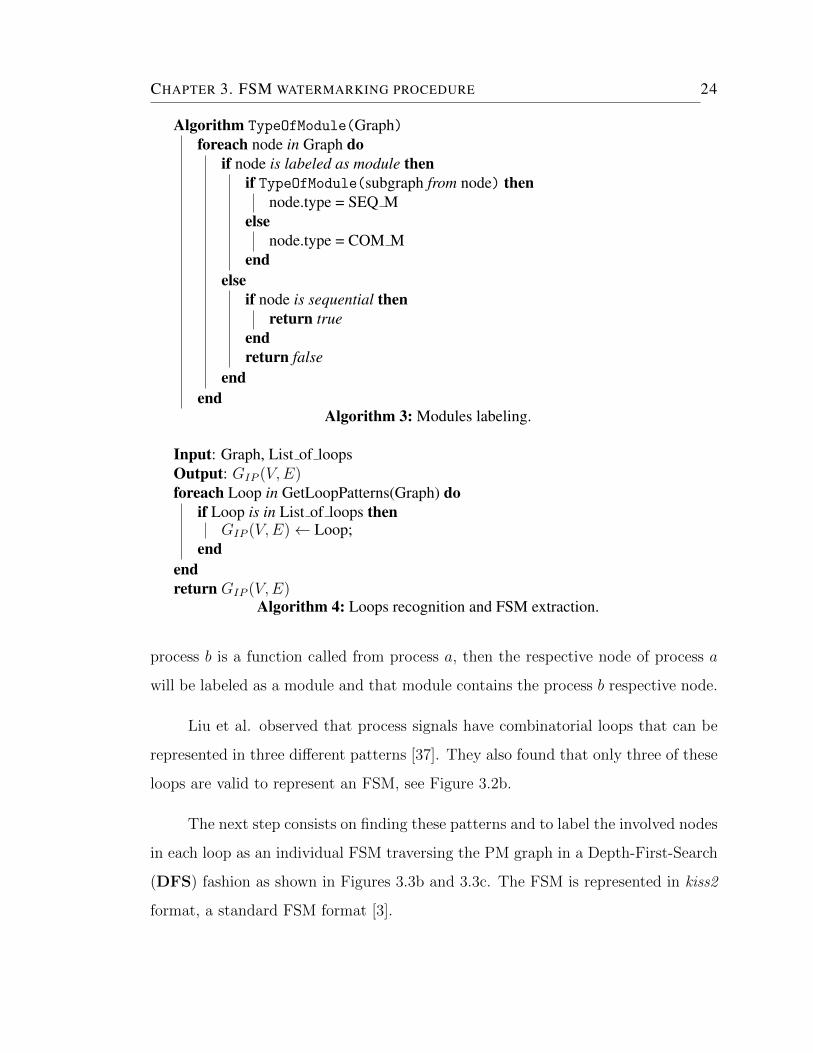
VHDL description will be modeled as a hierarchical modular graph, where each
module will contain processes or more modules if necessary (see Figure 3.2a).
There are two different kinds of modules and processes, sequential and combi-
natorial. Modules with sequential label contain at least one sequential process, and
modules with combinatorial labels, do not contain any sequential process.
Each process at RTL is represented in a Process-Module (PM) graph by a node
as shown in Figure 3.3a. If there is a fanout or fanin from process a to process b, then
a direct transition between their respective nodes is assigned. On the other hand, if
CHAPTER 3. FSM WATERMARKING PROCEDURE 24
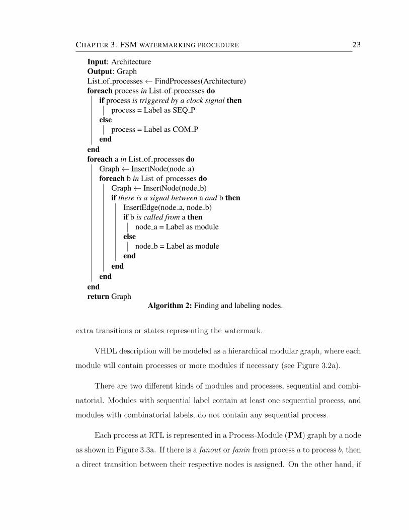
Algorithm TypeOfModule(Graph)foreach node in Graph do
if node is labeled as module thenif TypeOfModule(subgraph from node) then
node.type = SEQ Melse
node.type = COM Mend
elseif node is sequential then
return trueendreturn false
endend
Algorithm 3: Modules labeling.
Input: Graph, List of loopsOutput: GIP (V,E)foreach Loop in GetLoopPatterns(Graph) do
if Loop is in List of loops thenGIP (V,E)← Loop;
endendreturn GIP (V,E)
Algorithm 4: Loops recognition and FSM extraction.
process b is a function called from process a, then the respective node of process a
will be labeled as a module and that module contains the process b respective node.
Liu et al. observed that process signals have combinatorial loops that can be
represented in three different patterns [37]. They also found that only three of these
loops are valid to represent an FSM, see Figure 3.2b.
The next step consists on finding these patterns and to label the involved nodes
in each loop as an individual FSM traversing the PM graph in a Depth-First-Search
(DFS) fashion as shown in Figures 3.3b and 3.3c. The FSM is represented in kiss2
format, a standard FSM format [3].
CHAPTER 3. FSM WATERMARKING PROCEDURE 25
(a) Modules in HDL (b) Valid FSM loop patterns in RTL VHDL
Figure 3.2: Loop patterns
So far, one out of two FSMs that will be merged has been extracted. This FSM
represents the IP Core behavior, in the next section the translation from a file into
the second FSM that will represent the signature, and their subsequent merging will
be explained.
3.2 Proposed watermark translation
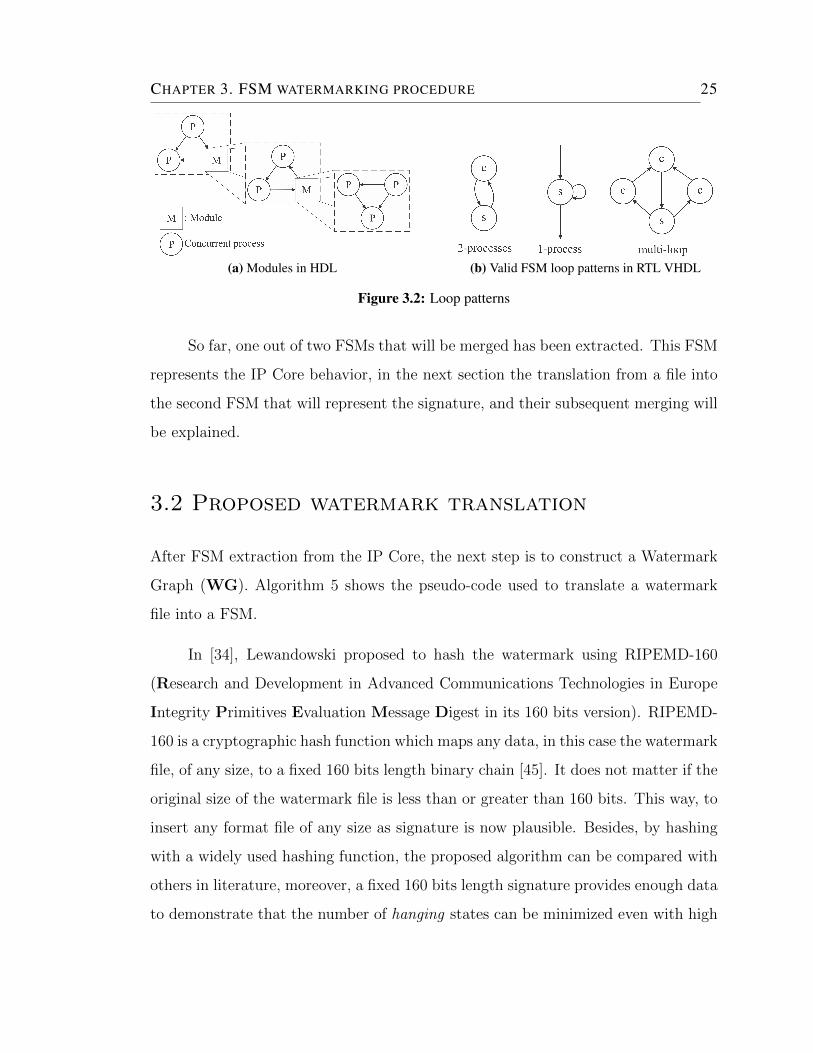
After FSM extraction from the IP Core, the next step is to construct a Watermark
Graph (WG). Algorithm 5 shows the pseudo-code used to translate a watermark
file into a FSM.
In [34], Lewandowski proposed to hash the watermark using RIPEMD-160
(Research and Development in Advanced Communications Technologies in Europe
Integrity Primitives Evaluation Message Digest in its 160 bits version). RIPEMD-
160 is a cryptographic hash function which maps any data, in this case the watermark
file, of any size, to a fixed 160 bits length binary chain [45]. It does not matter if the
original size of the watermark file is less than or greater than 160 bits. This way, to
insert any format file of any size as signature is now plausible. Besides, by hashing
with a widely used hashing function, the proposed algorithm can be compared with
others in literature, moreover, a fixed 160 bits length signature provides enough data
to demonstrate that the number of hanging states can be minimized even with high

CHAPTER 3. FSM WATERMARKING PROCEDURE 26
(a) Original PM graph (b) PM graph loop patterns
(c) Final PM graph FSMs
Figure 3.3: Loop patterns and FSM recognition
CHAPTER 3. FSM WATERMARKING PROCEDURE 27
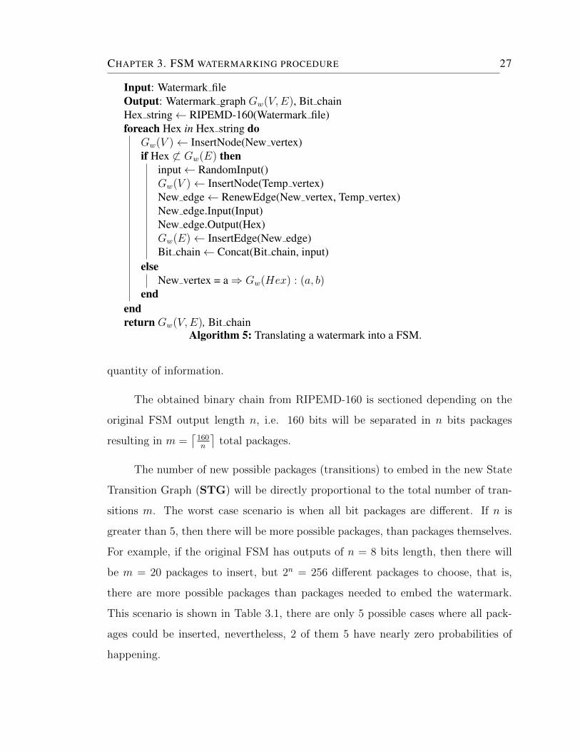
Input: Watermark fileOutput: Watermark graph Gw(V,E), Bit chainHex string← RIPEMD-160(Watermark file)foreach Hex in Hex string do
Gw(V )← InsertNode(New vertex)if Hex 6⊂ Gw(E) then
input← RandomInput()Gw(V )← InsertNode(Temp vertex)New edge← RenewEdge(New vertex, Temp vertex)New edge.Input(Input)New edge.Output(Hex)Gw(E)← InsertEdge(New edge)Bit chain← Concat(Bit chain, input)
elseNew vertex = a⇒ Gw(Hex) : (a, b)
endendreturn Gw(V,E), Bit chain
Algorithm 5: Translating a watermark into a FSM.
quantity of information.
The obtained binary chain from RIPEMD-160 is sectioned depending on the
original FSM output length n, i.e. 160 bits will be separated in n bits packages
resulting in m =⌈160n
⌉total packages.
The number of new possible packages (transitions) to embed in the new State
Transition Graph (STG) will be directly proportional to the total number of tran-
sitions m. The worst case scenario is when all bit packages are different. If n is
greater than 5, then there will be more possible packages, than packages themselves.
For example, if the original FSM has outputs of n = 8 bits length, then there will
be m = 20 packages to insert, but 2n = 256 different packages to choose, that is,
there are more possible packages than packages needed to embed the watermark.
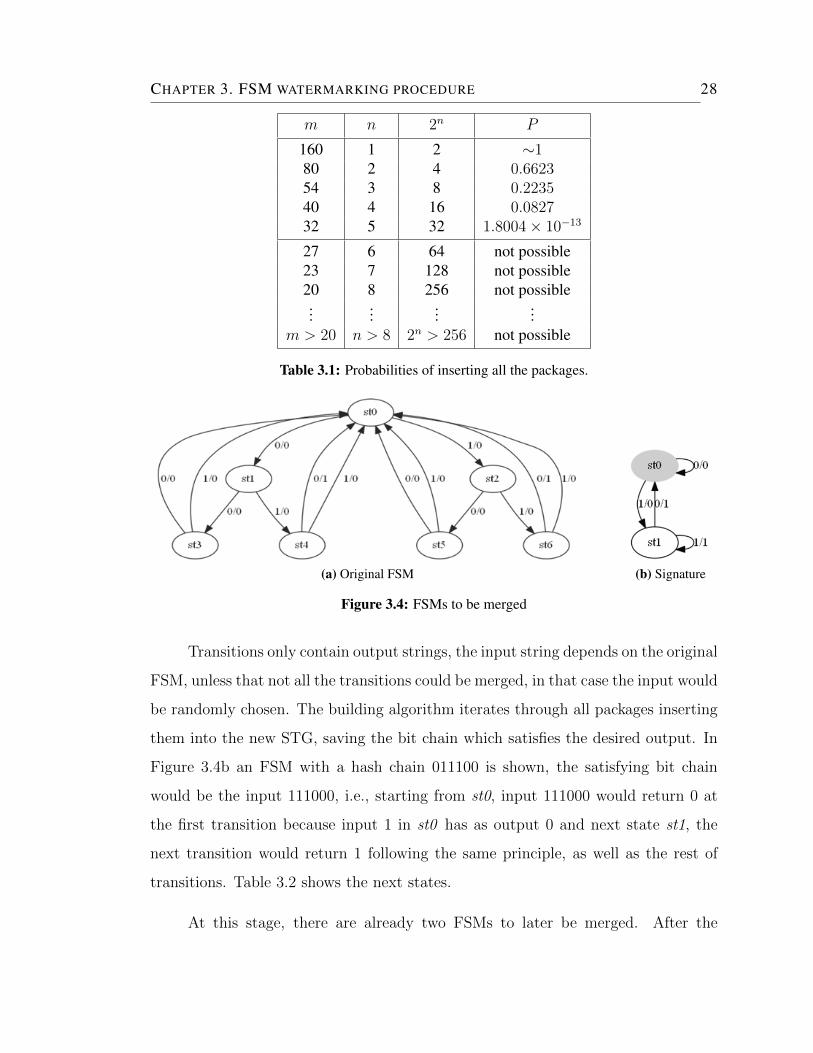
This scenario is shown in Table 3.1, there are only 5 possible cases where all pack-
ages could be inserted, nevertheless, 2 of them 5 have nearly zero probabilities of
happening.
CHAPTER 3. FSM WATERMARKING PROCEDURE 28
m n 2n P
160 1 2 ∼180 2 4 0.662354 3 8 0.223540 4 16 0.082732 5 32 1.8004× 10⁻¹³
27 6 64 not possible23 7 128 not possible20 8 256 not possible...
......
...m > 20 n > 8 2n > 256 not possible
Table 3.1: Probabilities of inserting all the packages.
(a) Original FSM (b) Signature
Figure 3.4: FSMs to be merged
Transitions only contain output strings, the input string depends on the original
FSM, unless that not all the transitions could be merged, in that case the input would
be randomly chosen. The building algorithm iterates through all packages inserting
them into the new STG, saving the bit chain which satisfies the desired output. In
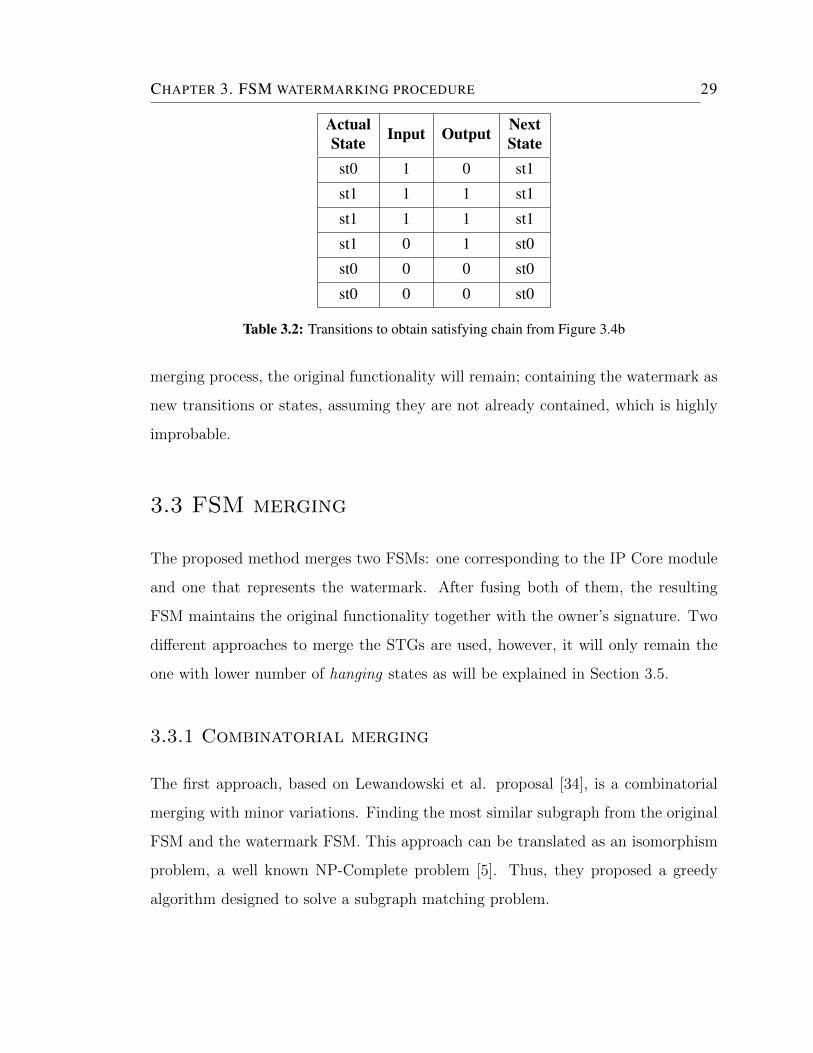
Figure 3.4b an FSM with a hash chain 011100 is shown, the satisfying bit chain
would be the input 111000, i.e., starting from st0, input 111000 would return 0 at
the first transition because input 1 in st0 has as output 0 and next state st1, the
next transition would return 1 following the same principle, as well as the rest of
transitions. Table 3.2 shows the next states.
At this stage, there are already two FSMs to later be merged. After the
CHAPTER 3. FSM WATERMARKING PROCEDURE 29
Actual Input Output NextState Statest0 1 0 st1
st1 1 1 st1
st1 1 1 st1
st1 0 1 st0
st0 0 0 st0
st0 0 0 st0
Table 3.2: Transitions to obtain satisfying chain from Figure 3.4b
merging process, the original functionality will remain; containing the watermark as
new transitions or states, assuming they are not already contained, which is highly
improbable.
3.3 FSM merging
The proposed method merges two FSMs: one corresponding to the IP Core module
and one that represents the watermark. After fusing both of them, the resulting
FSM maintains the original functionality together with the owner’s signature. Two
different approaches to merge the STGs are used, however, it will only remain the
one with lower number of hanging states as will be explained in Section 3.5.
3.3.1 Combinatorial merging
The first approach, based on Lewandowski et al. proposal [34], is a combinatorial
merging with minor variations. Finding the most similar subgraph from the original
FSM and the watermark FSM. This approach can be translated as an isomorphism
problem, a well known NP-Complete problem [5]. Thus, they proposed a greedy
algorithm designed to solve a subgraph matching problem.
CHAPTER 3. FSM WATERMARKING PROCEDURE 30
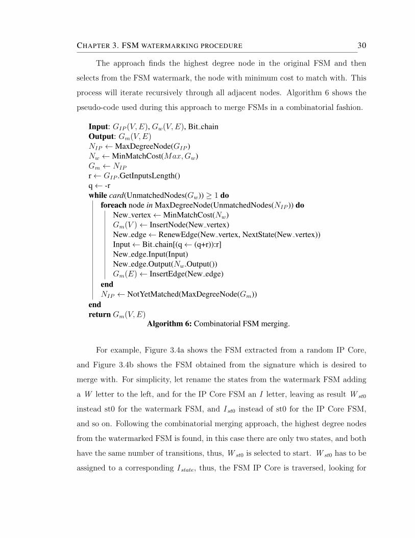
The approach finds the highest degree node in the original FSM and then
selects from the FSM watermark, the node with minimum cost to match with. This
process will iterate recursively through all adjacent nodes. Algorithm 6 shows the
pseudo-code used during this approach to merge FSMs in a combinatorial fashion.
Input: GIP (V,E), Gw(V,E), Bit chainOutput: Gm(V,E)NIP ←MaxDegreeNode(GIP )Nw ←MinMatchCost(Max,Gw)Gm ← NIP
r← GIP .GetInputsLength()q← -rwhile card(UnmatchedNodes(Gw)) ≥ 1 do
foreach node in MaxDegreeNode(UnmatchedNodes(NIP )) doNew vertex←MinMatchCost(Nw)Gm(V )← InsertNode(New vertex)New edge← RenewEdge(New vertex, NextState(New vertex))Input← Bit chain[(q← (q+r)):r]New edge.Input(Input)New edge.Output(Nw.Output())Gm(E)← InsertEdge(New edge)
endNIP ← NotYetMatched(MaxDegreeNode(Gm))
endreturn Gm(V,E)
Algorithm 6: Combinatorial FSM merging.
For example, Figure 3.4a shows the FSM extracted from a random IP Core,
and Figure 3.4b shows the FSM obtained from the signature which is desired to
merge with. For simplicity, let rename the states from the watermark FSM adding
a W letter to the left, and for the IP Core FSM an I letter, leaving as result W st0
instead st0 for the watermark FSM, and I st0 instead of st0 for the IP Core FSM,
and so on. Following the combinatorial merging approach, the highest degree nodes
from the watermarked FSM is found, in this case there are only two states, and both
have the same number of transitions, thus, W st0 is selected to start. W st0 has to be
assigned to a corresponding I state, thus, the FSM IP Core is traversed, looking for
CHAPTER 3. FSM WATERMARKING PROCEDURE 31
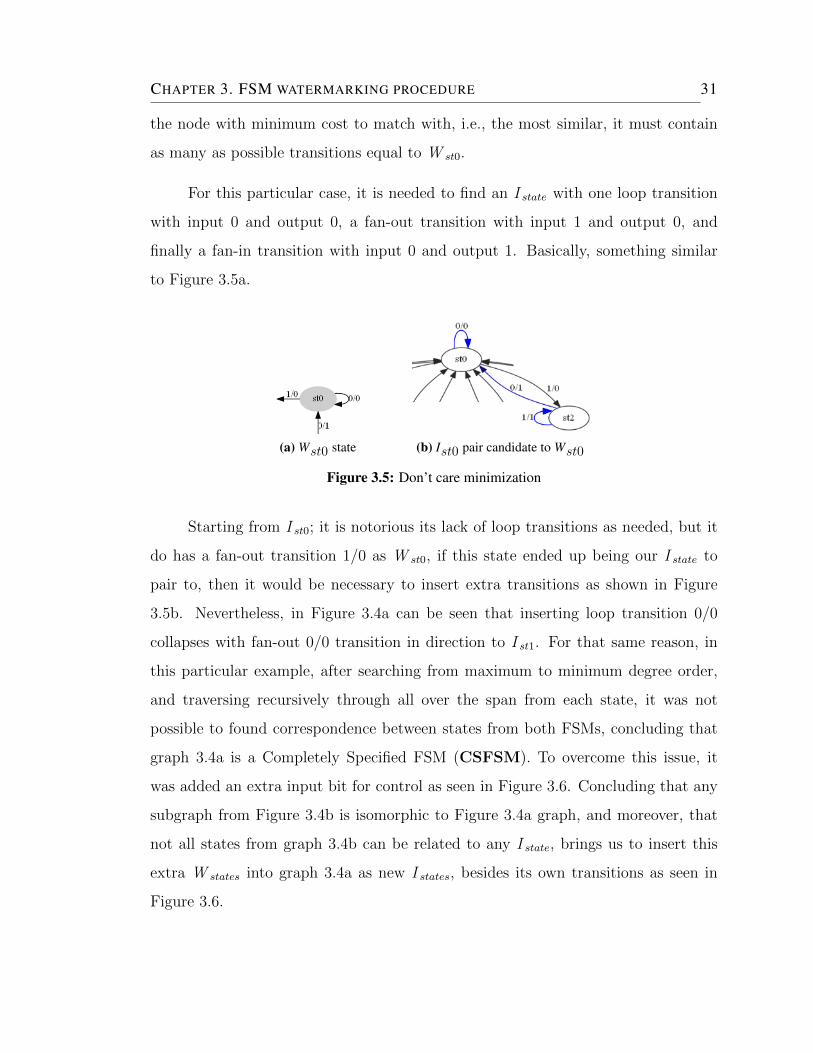
the node with minimum cost to match with, i.e., the most similar, it must contain
as many as possible transitions equal to W st0.
For this particular case, it is needed to find an I state with one loop transition
with input 0 and output 0, a fan-out transition with input 1 and output 0, and
finally a fan-in transition with input 0 and output 1. Basically, something similar
to Figure 3.5a.
(a) Wst0 state (b) Ist0 pair candidate to Wst0
Figure 3.5: Don’t care minimization
Starting from I st0; it is notorious its lack of loop transitions as needed, but it
do has a fan-out transition 1/0 as W st0, if this state ended up being our I state to
pair to, then it would be necessary to insert extra transitions as shown in Figure
3.5b. Nevertheless, in Figure 3.4a can be seen that inserting loop transition 0/0
collapses with fan-out 0/0 transition in direction to I st1. For that same reason, in
this particular example, after searching from maximum to minimum degree order,
and traversing recursively through all over the span from each state, it was not
possible to found correspondence between states from both FSMs, concluding that
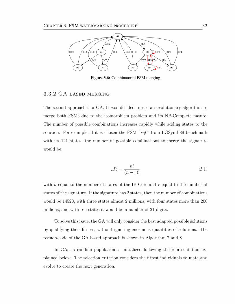
graph 3.4a is a Completely Specified FSM (CSFSM). To overcome this issue, it
was added an extra input bit for control as seen in Figure 3.6. Concluding that any
subgraph from Figure 3.4b is isomorphic to Figure 3.4a graph, and moreover, that
not all states from graph 3.4b can be related to any I state, brings us to insert this
extra W states into graph 3.4a as new I states, besides its own transitions as seen in
Figure 3.6.
CHAPTER 3. FSM WATERMARKING PROCEDURE 32
Figure 3.6: Combinatorial FSM merging
3.3.2 GA based merging
The second approach is a GA. It was decided to use an evolutionary algorithm to
merge both FSMs due to the isomorphism problem and its NP-Complete nature.
The number of possible combinations increases rapidly while adding states to the
solution. For example, if it is chosen the FSM “scf ” from LGSynth89 benchmark
with its 121 states, the number of possible combinations to merge the signature
would be:
nPr =n!
(n− r)!(3.1)
with n equal to the number of states of the IP Core and r equal to the number of
states of the signature. If the signature has 2 states, then the number of combinations
would be 14520, with three states almost 2 millions, with four states more than 200
millions, and with ten states it would be a number of 21 digits.
To solve this issue, the GA will only consider the best adapted possible solutions
by qualifying their fitness, without ignoring enormous quantities of solutions. The
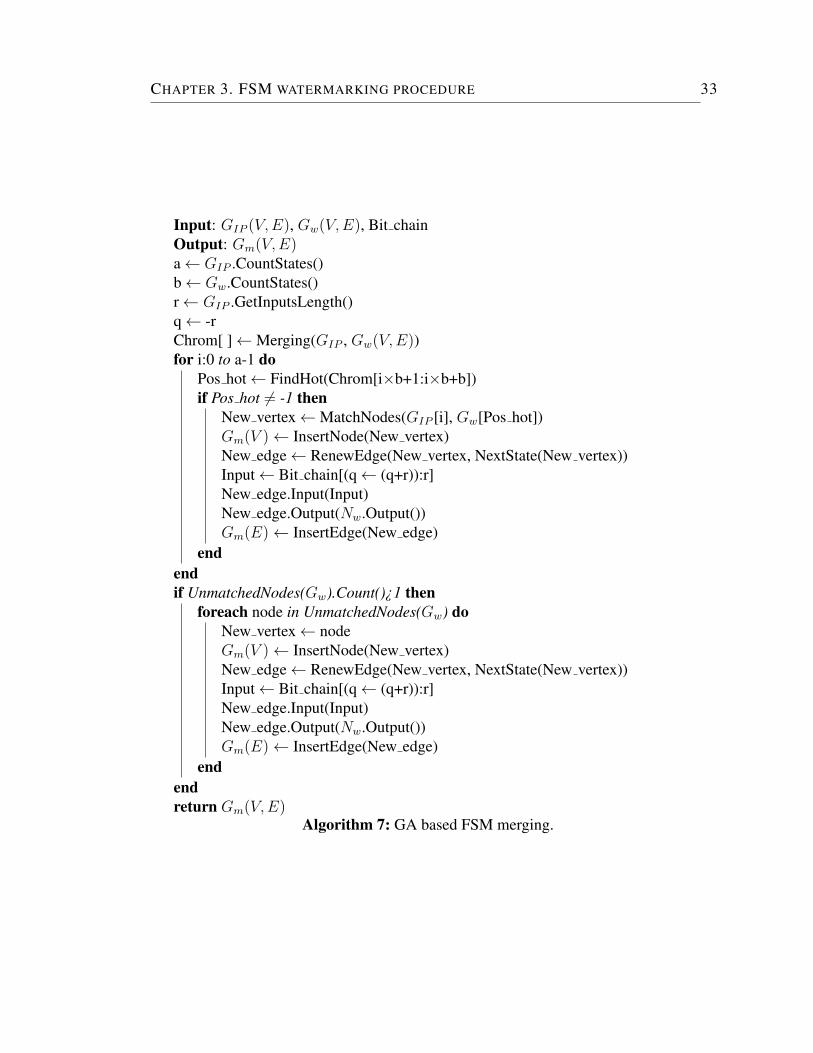
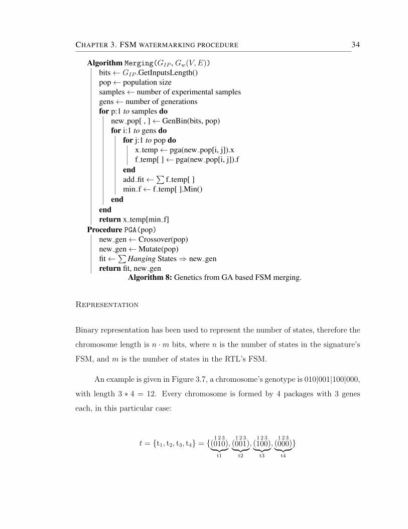
pseudo-code of the GA based approach is shown in Algorithm 7 and 8.
In GAs, a random population is initialized following the representation ex-
plained below. The selection criterion considers the fittest individuals to mate and
evolve to create the next generation.
CHAPTER 3. FSM WATERMARKING PROCEDURE 33
Input: GIP (V,E), Gw(V,E), Bit chainOutput: Gm(V,E)a← GIP .CountStates()b← Gw.CountStates()r← GIP .GetInputsLength()q← -rChrom[ ]←Merging(GIP , Gw(V,E))for i:0 to a-1 do
Pos hot← FindHot(Chrom[i×b+1:i×b+b])if Pos hot 6= -1 then
New vertex←MatchNodes(GIP [i], Gw[Pos hot])Gm(V )← InsertNode(New vertex)New edge← RenewEdge(New vertex, NextState(New vertex))Input← Bit chain[(q← (q+r)):r]New edge.Input(Input)New edge.Output(Nw.Output())Gm(E)← InsertEdge(New edge)
endendif UnmatchedNodes(Gw).Count()¿1 then
foreach node in UnmatchedNodes(Gw) doNew vertex← nodeGm(V )← InsertNode(New vertex)New edge← RenewEdge(New vertex, NextState(New vertex))Input← Bit chain[(q← (q+r)):r]New edge.Input(Input)New edge.Output(Nw.Output())Gm(E)← InsertEdge(New edge)
endendreturn Gm(V,E)
Algorithm 7: GA based FSM merging.
CHAPTER 3. FSM WATERMARKING PROCEDURE 34
Algorithm Merging(GIP , Gw(V,E))bits← GIP .GetInputsLength()pop← population sizesamples← number of experimental samplesgens← number of generationsfor p:1 to samples do
new pop[ , ]← GenBin(bits, pop)for i:1 to gens do
for j:1 to pop dox temp← pga(new pop[i, j]).xf temp[ ]← pga(new pop[i, j]).f
endadd fit←
∑f temp[ ]
min f← f temp[ ].Min()end
endreturn x temp[min f]
Procedure PGA(pop)new gen← Crossover(pop)new gen←Mutate(pop)fit←
∑Hanging States⇒ new gen
return fit, new genAlgorithm 8: Genetics from GA based FSM merging.
Representation
Binary representation has been used to represent the number of states, therefore the
chromosome length is n ·m bits, where n is the number of states in the signature’s
FSM, and m is the number of states in the RTL’s FSM.
An example is given in Figure 3.7, a chromosome’s genotype is 010|001|100|000,
with length 3 ∗ 4 = 12. Every chromosome is formed by 4 packages with 3 genes
each, in this particular case:
t = {t1, t2, t3, t4} = {(1
02
13
0)︸ ︷︷ ︸t1
, (1
02
03
1)︸ ︷︷ ︸t2
, (1
12
03
0)︸ ︷︷ ︸t3
, (1
02
03
0)︸ ︷︷ ︸t4
}
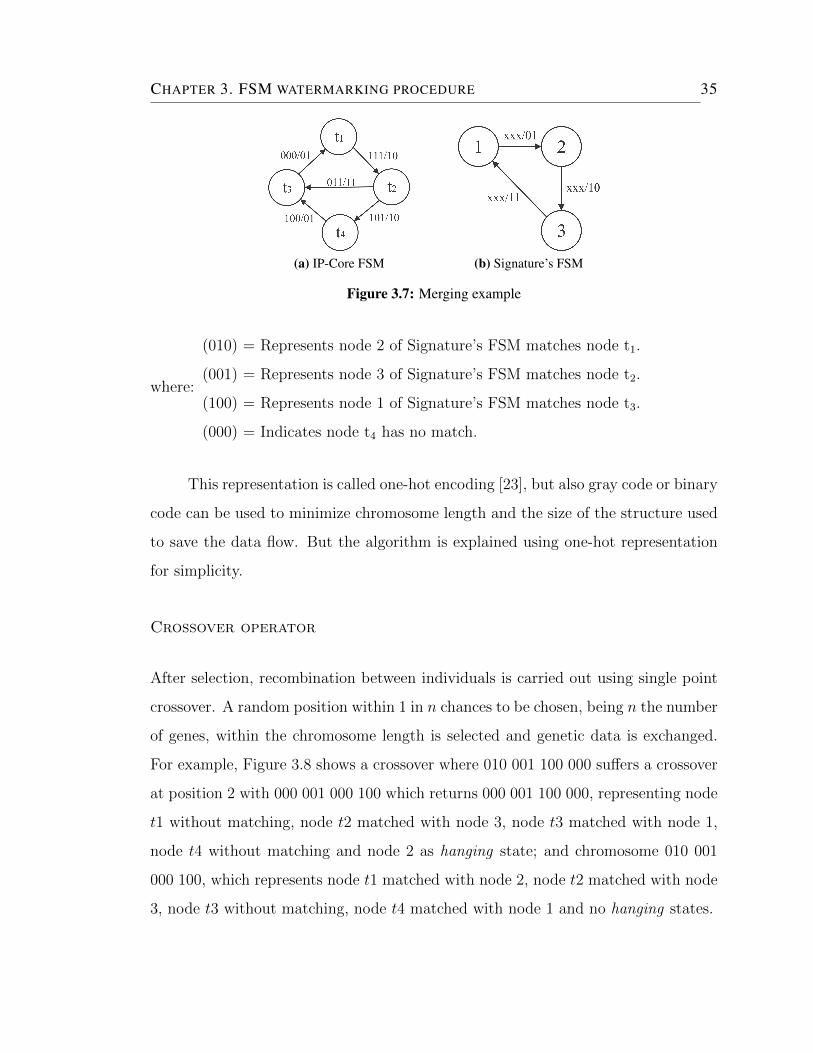
CHAPTER 3. FSM WATERMARKING PROCEDURE 35
(a) IP-Core FSM (b) Signature’s FSM
Figure 3.7: Merging example
where:
(010) = Represents node 2 of Signature’s FSM matches node t1.
(001) = Represents node 3 of Signature’s FSM matches node t2.
(100) = Represents node 1 of Signature’s FSM matches node t3.
(000) = Indicates node t4 has no match.
This representation is called one-hot encoding [23], but also gray code or binary
code can be used to minimize chromosome length and the size of the structure used
to save the data flow. But the algorithm is explained using one-hot representation
for simplicity.
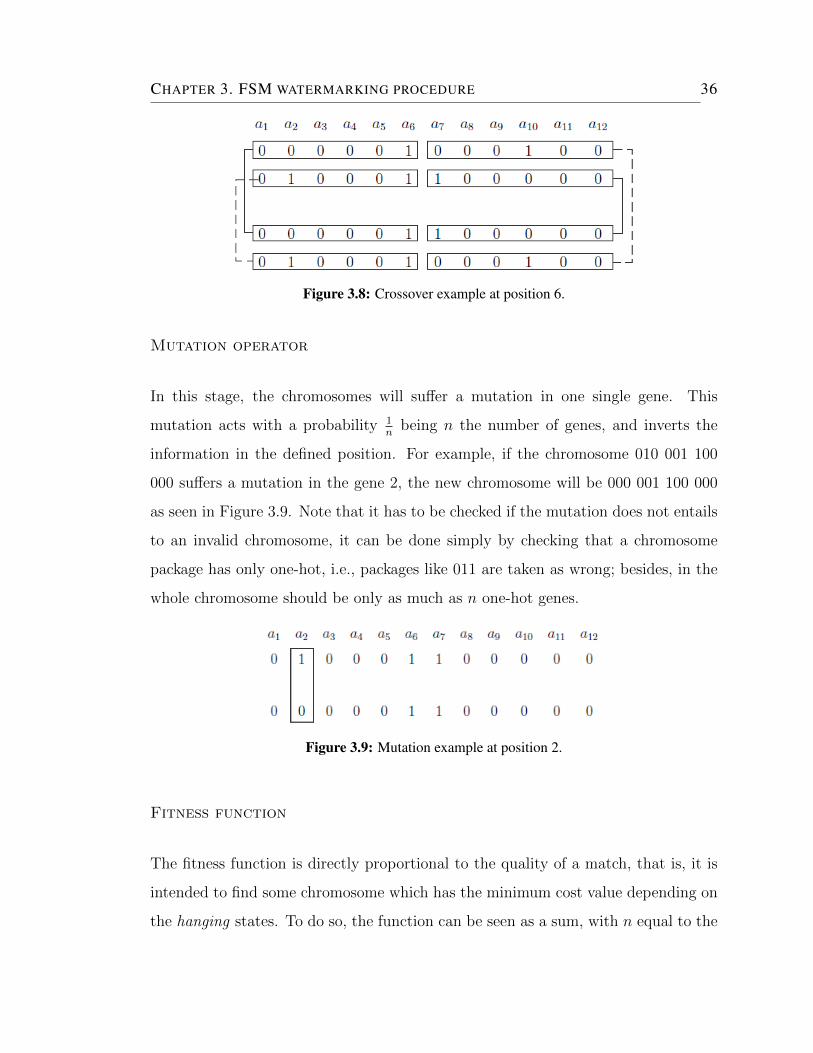
Crossover operator
After selection, recombination between individuals is carried out using single point
crossover. A random position within 1 in n chances to be chosen, being n the number
of genes, within the chromosome length is selected and genetic data is exchanged.
For example, Figure 3.8 shows a crossover where 010 001 100 000 suffers a crossover
at position 2 with 000 001 000 100 which returns 000 001 100 000, representing node
t1 without matching, node t2 matched with node 3, node t3 matched with node 1,
node t4 without matching and node 2 as hanging state; and chromosome 010 001
000 100, which represents node t1 matched with node 2, node t2 matched with node
3, node t3 without matching, node t4 matched with node 1 and no hanging states.
CHAPTER 3. FSM WATERMARKING PROCEDURE 36
Figure 3.8: Crossover example at position 6.
Mutation operator
In this stage, the chromosomes will suffer a mutation in one single gene. This
mutation acts with a probability 1n
being n the number of genes, and inverts the
information in the defined position. For example, if the chromosome 010 001 100
000 suffers a mutation in the gene 2, the new chromosome will be 000 001 100 000
as seen in Figure 3.9. Note that it has to be checked if the mutation does not entails
to an invalid chromosome, it can be done simply by checking that a chromosome
package has only one-hot, i.e., packages like 011 are taken as wrong; besides, in the
whole chromosome should be only as much as n one-hot genes.
Figure 3.9: Mutation example at position 2.
Fitness function
The fitness function is directly proportional to the quality of a match, that is, it is
intended to find some chromosome which has the minimum cost value depending on
the hanging states. To do so, the function can be seen as a sum, with n equal to the
CHAPTER 3. FSM WATERMARKING PROCEDURE 37
number of hanging statesn∑i=1
i. In other words, it is intended to reduce the number
of hanging states.
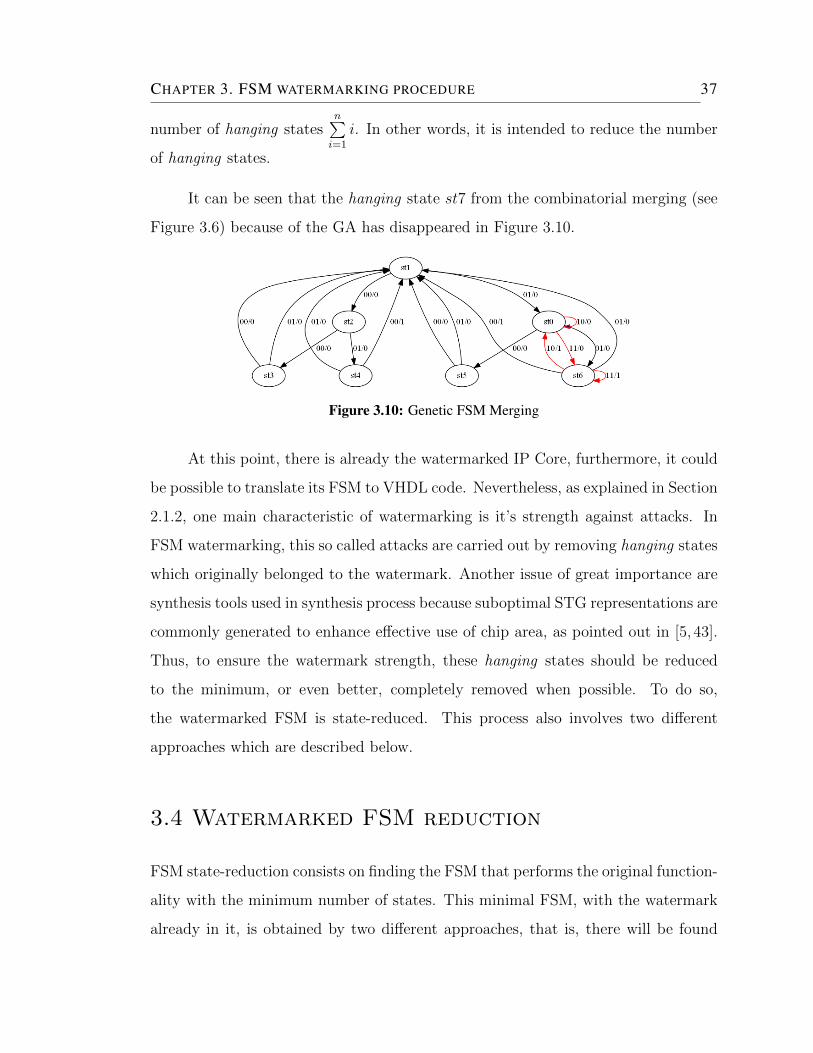
It can be seen that the hanging state st7 from the combinatorial merging (see
Figure 3.6) because of the GA has disappeared in Figure 3.10.
Figure 3.10: Genetic FSM Merging
At this point, there is already the watermarked IP Core, furthermore, it could
be possible to translate its FSM to VHDL code. Nevertheless, as explained in Section
2.1.2, one main characteristic of watermarking is it’s strength against attacks. In
FSM watermarking, this so called attacks are carried out by removing hanging states
which originally belonged to the watermark. Another issue of great importance are
synthesis tools used in synthesis process because suboptimal STG representations are
commonly generated to enhance effective use of chip area, as pointed out in [5, 43].
Thus, to ensure the watermark strength, these hanging states should be reduced
to the minimum, or even better, completely removed when possible. To do so,
the watermarked FSM is state-reduced. This process also involves two different
approaches which are described below.
3.4 Watermarked FSM reduction
FSM state-reduction consists on finding the FSM that performs the original function-
ality with the minimum number of states. This minimal FSM, with the watermark
already in it, is obtained by two different approaches, that is, there will be found
CHAPTER 3. FSM WATERMARKING PROCEDURE 38
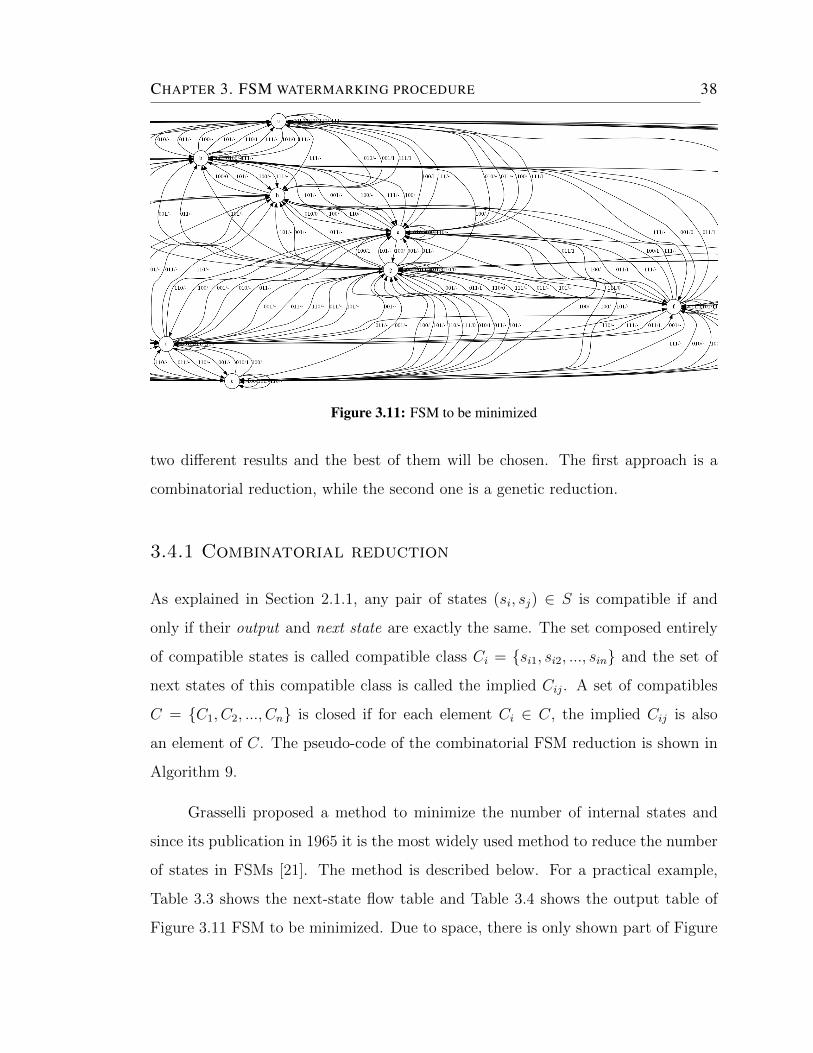
Figure 3.11: FSM to be minimized
two different results and the best of them will be chosen. The first approach is a
combinatorial reduction, while the second one is a genetic reduction.
3.4.1 Combinatorial reduction
As explained in Section 2.1.1, any pair of states (si, sj) ∈ S is compatible if and
only if their output and next state are exactly the same. The set composed entirely
of compatible states is called compatible class Ci = {si1, si2, ..., sin} and the set of
next states of this compatible class is called the implied Cij. A set of compatibles
C = {C1, C2, ..., Cn} is closed if for each element Ci ∈ C, the implied Cij is also
an element of C. The pseudo-code of the combinatorial FSM reduction is shown in
Algorithm 9.
Grasselli proposed a method to minimize the number of internal states and
since its publication in 1965 it is the most widely used method to reduce the number
of states in FSMs [21]. The method is described below. For a practical example,
Table 3.3 shows the next-state flow table and Table 3.4 shows the output table of
Figure 3.11 FSM to be minimized. Due to space, there is only shown part of Figure
CHAPTER 3. FSM WATERMARKING PROCEDURE 39
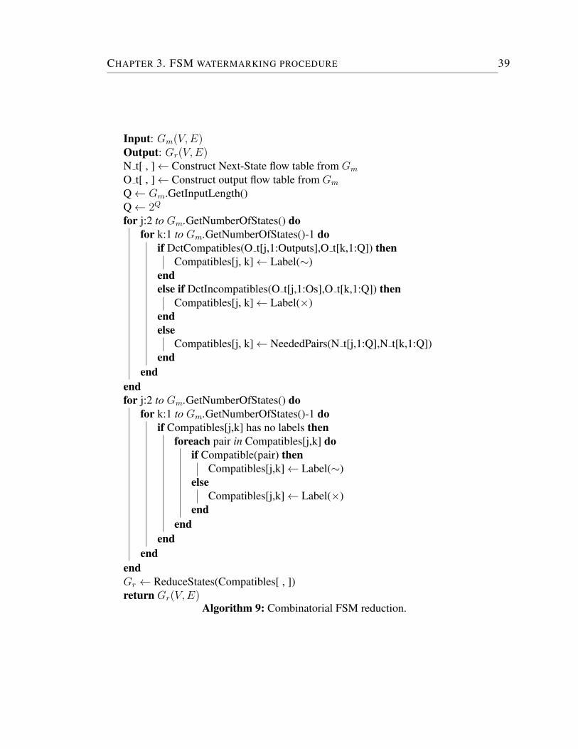
Input: Gm(V,E)Output: Gr(V,E)N t[ , ]← Construct Next-State flow table from Gm
O t[ , ]← Construct output flow table from Gm
Q← Gm.GetInputLength()Q← 2Q
for j:2 to Gm.GetNumberOfStates() dofor k:1 to Gm.GetNumberOfStates()-1 do
if DctCompatibles(O t[j,1:Outputs],O t[k,1:Q]) thenCompatibles[j, k]← Label(∼)
endelse if DctIncompatibles(O t[j,1:Os],O t[k,1:Q]) then
Compatibles[j, k]← Label(×)endelse
Compatibles[j, k]← NeededPairs(N t[j,1:Q],N t[k,1:Q])end
endendfor j:2 to Gm.GetNumberOfStates() do
for k:1 to Gm.GetNumberOfStates()-1 doif Compatibles[j,k] has no labels then
foreach pair in Compatibles[j,k] doif Compatible(pair) then
Compatibles[j,k]← Label(∼)else
Compatibles[j,k]← Label(×)end
endend
endendGr ← ReduceStates(Compatibles[ , ])return Gr(V,E)
Algorithm 9: Combinatorial FSM reduction.
CHAPTER 3. FSM WATERMARKING PROCEDURE 40
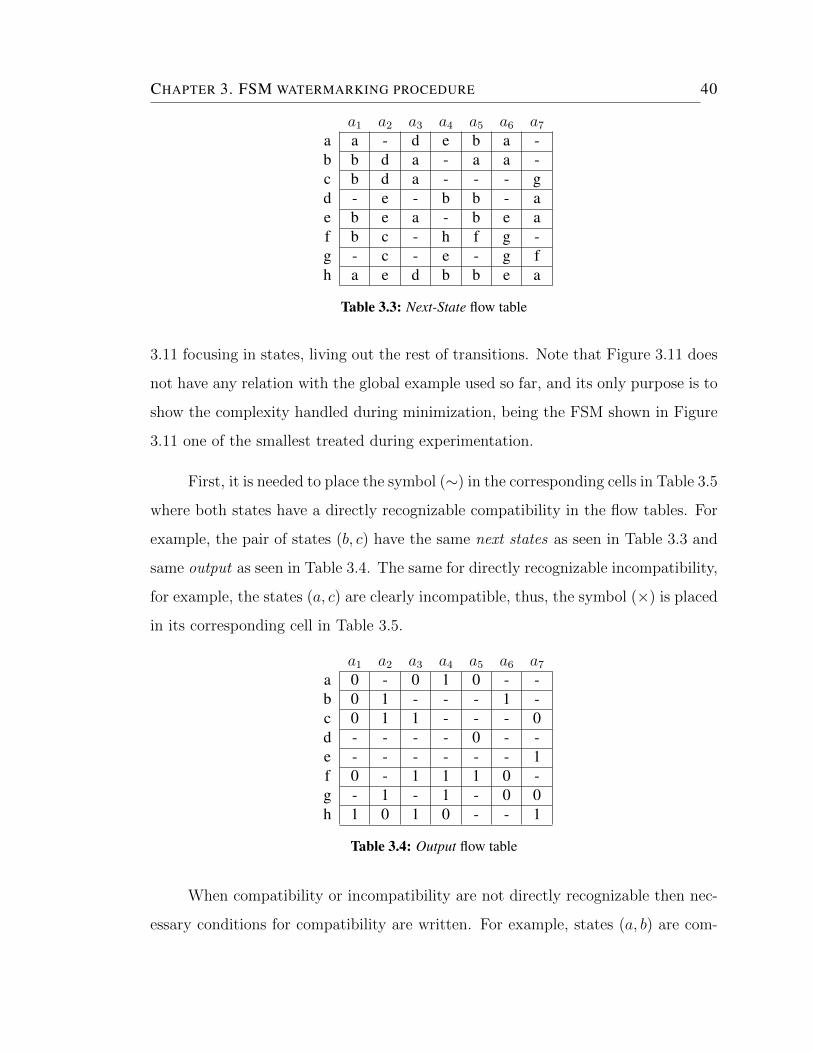
a1 a2 a3 a4 a5 a6 a7a a - d e b a -b b d a - a a -c b d a - - - gd - e - b b - ae b e a - b e af b c - h f g -g - c - e - g fh a e d b b e a
Table 3.3: Next-State flow table
3.11 focusing in states, living out the rest of transitions. Note that Figure 3.11 does
not have any relation with the global example used so far, and its only purpose is to
show the complexity handled during minimization, being the FSM shown in Figure
3.11 one of the smallest treated during experimentation.
First, it is needed to place the symbol (∼) in the corresponding cells in Table 3.5
where both states have a directly recognizable compatibility in the flow tables. For
example, the pair of states (b, c) have the same next states as seen in Table 3.3 and
same output as seen in Table 3.4. The same for directly recognizable incompatibility,
for example, the states (a, c) are clearly incompatible, thus, the symbol (×) is placed
in its corresponding cell in Table 3.5.
a1 a2 a3 a4 a5 a6 a7a 0 - 0 1 0 - -b 0 1 - - - 1 -c 0 1 1 - - - 0d - - - - 0 - -e - - - - - - 1f 0 - 1 1 1 0 -g - 1 - 1 - 0 0h 1 0 1 0 - - 1
Table 3.4: Output flow table
When compatibility or incompatibility are not directly recognizable then nec-
essary conditions for compatibility are written. For example, states (a, b) are com-
CHAPTER 3. FSM WATERMARKING PROCEDURE 41
patible only if states (d, a) are compatible also, thus, this new pair is written in the
cell shared by b and a.
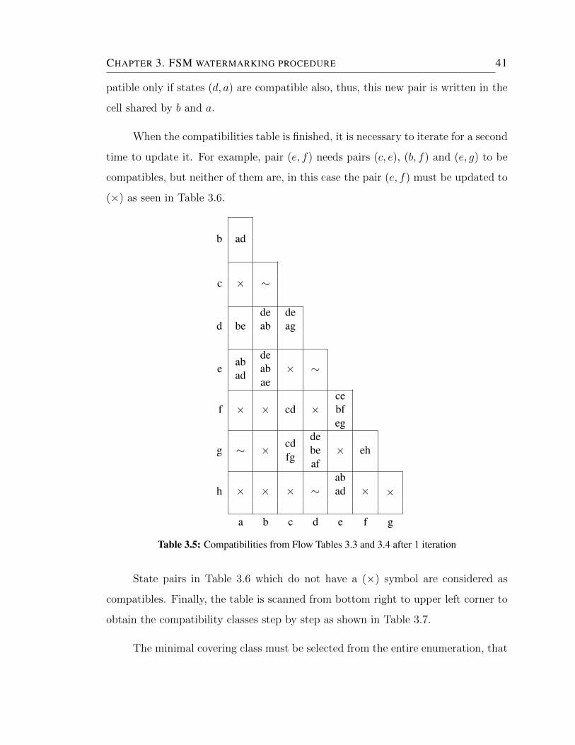
When the compatibilities table is finished, it is necessary to iterate for a second
time to update it. For example, pair (e, f) needs pairs (c, e), (b, f) and (e, g) to be
compatibles, but neither of them are, in this case the pair (e, f) must be updated to
(×) as seen in Table 3.6.
b ad
c × ∼
d bedeab
deag
eabad
deabae
× ∼
f × × cd ×cebfeg
g ∼ × cdfg
debeaf
× eh
h × × × ∼abad × ×
a b c d e f g
Table 3.5: Compatibilities from Flow Tables 3.3 and 3.4 after 1 iteration
State pairs in Table 3.6 which do not have a (×) symbol are considered as
compatibles. Finally, the table is scanned from bottom right to upper left corner to
obtain the compatibility classes step by step as shown in Table 3.7.
The minimal covering class must be selected from the entire enumeration, that
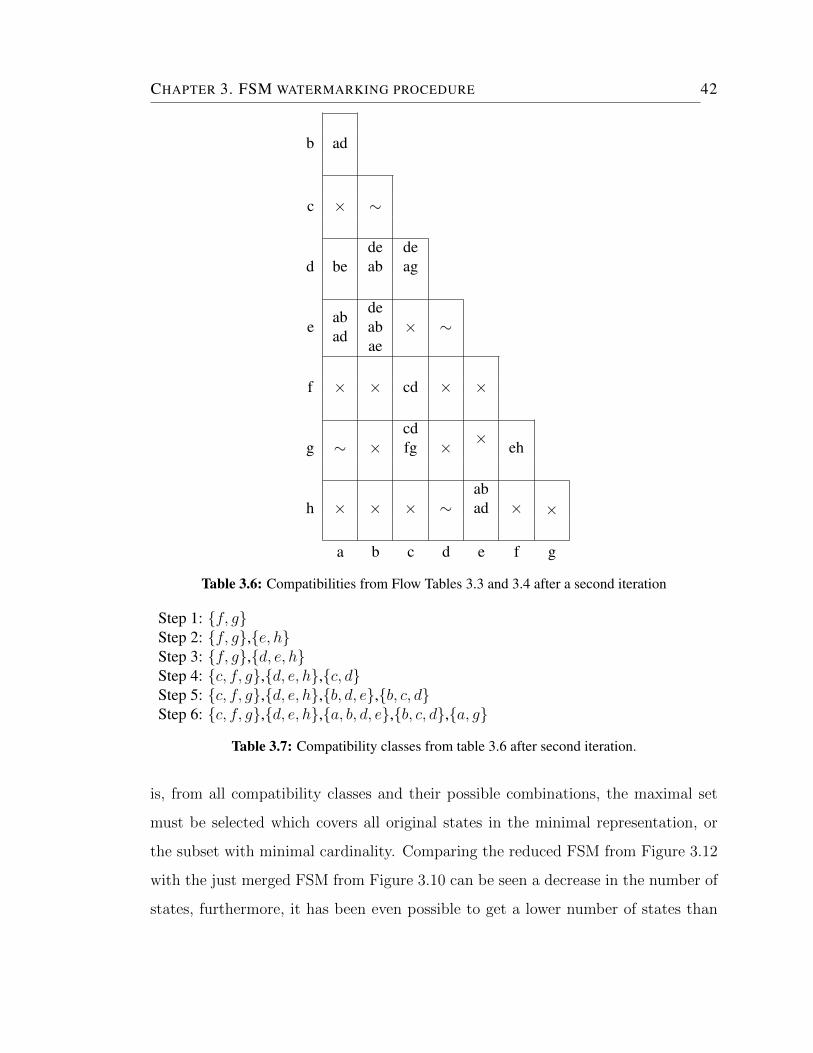
CHAPTER 3. FSM WATERMARKING PROCEDURE 42
b ad
c × ∼
d bedeab
deag
eabad
deabae
× ∼
f × × cd × ×
g ∼ ×cdfg × × eh
h × × × ∼abad × ×
a b c d e f g
Table 3.6: Compatibilities from Flow Tables 3.3 and 3.4 after a second iteration
Step 1: {f, g}Step 2: {f, g},{e, h}Step 3: {f, g},{d, e, h}Step 4: {c, f, g},{d, e, h},{c, d}Step 5: {c, f, g},{d, e, h},{b, d, e},{b, c, d}Step 6: {c, f, g},{d, e, h},{a, b, d, e},{b, c, d},{a, g}
Table 3.7: Compatibility classes from table 3.6 after second iteration.
is, from all compatibility classes and their possible combinations, the maximal set
must be selected which covers all original states in the minimal representation, or
the subset with minimal cardinality. Comparing the reduced FSM from Figure 3.12
with the just merged FSM from Figure 3.10 can be seen a decrease in the number of
states, furthermore, it has been even possible to get a lower number of states than
CHAPTER 3. FSM WATERMARKING PROCEDURE 43
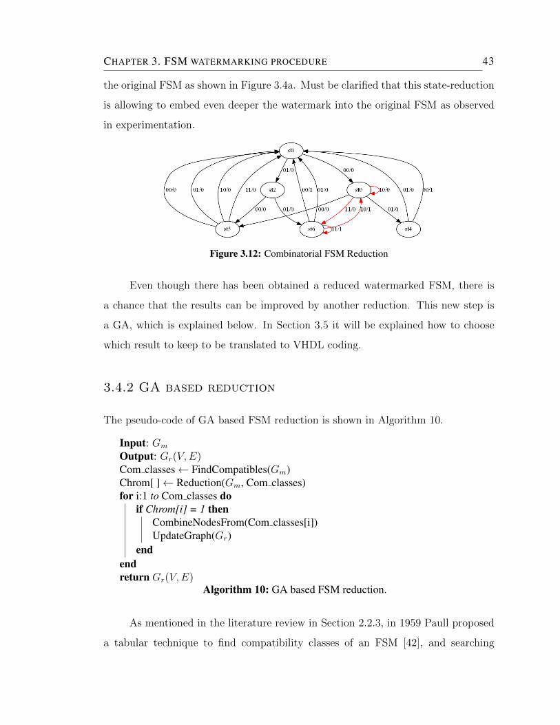
the original FSM as shown in Figure 3.4a. Must be clarified that this state-reduction
is allowing to embed even deeper the watermark into the original FSM as observed
in experimentation.
Figure 3.12: Combinatorial FSM Reduction
Even though there has been obtained a reduced watermarked FSM, there is
a chance that the results can be improved by another reduction. This new step is
a GA, which is explained below. In Section 3.5 it will be explained how to choose
which result to keep to be translated to VHDL coding.
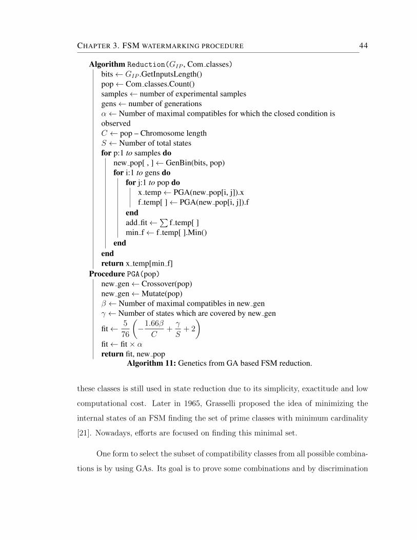
3.4.2 GA based reduction
The pseudo-code of GA based FSM reduction is shown in Algorithm 10.
Input: Gm
Output: Gr(V,E)Com classes← FindCompatibles(Gm)Chrom[ ]← Reduction(Gm, Com classes)for i:1 to Com classes do
if Chrom[i] = 1 thenCombineNodesFrom(Com classes[i])UpdateGraph(Gr)
endendreturn Gr(V,E)
Algorithm 10: GA based FSM reduction.
As mentioned in the literature review in Section 2.2.3, in 1959 Paull proposed
a tabular technique to find compatibility classes of an FSM [42], and searching
CHAPTER 3. FSM WATERMARKING PROCEDURE 44
Algorithm Reduction(GIP , Com classes)bits← GIP .GetInputsLength()pop← Com classes.Count()samples← number of experimental samplesgens← number of generationsα← Number of maximal compatibles for which the closed condition isobservedC ← pop – Chromosome lengthS ← Number of total statesfor p:1 to samples do
new pop[ , ]← GenBin(bits, pop)for i:1 to gens do
for j:1 to pop dox temp← PGA(new pop[i, j]).xf temp[ ]← PGA(new pop[i, j]).f
endadd fit←
∑f temp[ ]
min f← f temp[ ].Min()end
endreturn x temp[min f]
Procedure PGA(pop)new gen← Crossover(pop)new gen←Mutate(pop)β ← Number of maximal compatibles in new genγ ← Number of states which are covered by new gen
fit← 5
76
(−1.66β
C+γ
S+ 2
)fit← fit× αreturn fit, new pop
Algorithm 11: Genetics from GA based FSM reduction.
these classes is still used in state reduction due to its simplicity, exactitude and low
computational cost. Later in 1965, Grasselli proposed the idea of minimizing the
internal states of an FSM finding the set of prime classes with minimum cardinality
[21]. Nowadays, efforts are focused on finding this minimal set.
One form to select the subset of compatibility classes from all possible combina-
tions is by using GAs. Its goal is to prove some combinations and by discrimination
CHAPTER 3. FSM WATERMARKING PROCEDURE 45
Figure 3.13: Crossover example at position 3
to select the best ones and use some characteristics to create new generations of
possible solutions. Like Sanchez, the method proposed uses the same chromosome
representation and operators [48], nevertheless, in this research a new fitness function
that has shown a better performance is proposed.
Chromosomes
Any possible chromosome is represented as a binary string and its length is always
going to be the number of compatibility classes. For example, the chromosome
a1 a2 a3 a4 a5
0 0 1 1 0
represents the compatibility classes from Table 3.7 in step 6 ({a, b, d, e} and {b, c, d}),
note that classes {c, f, g}, {d, e, h}, and {a, g} would not be taken into account.
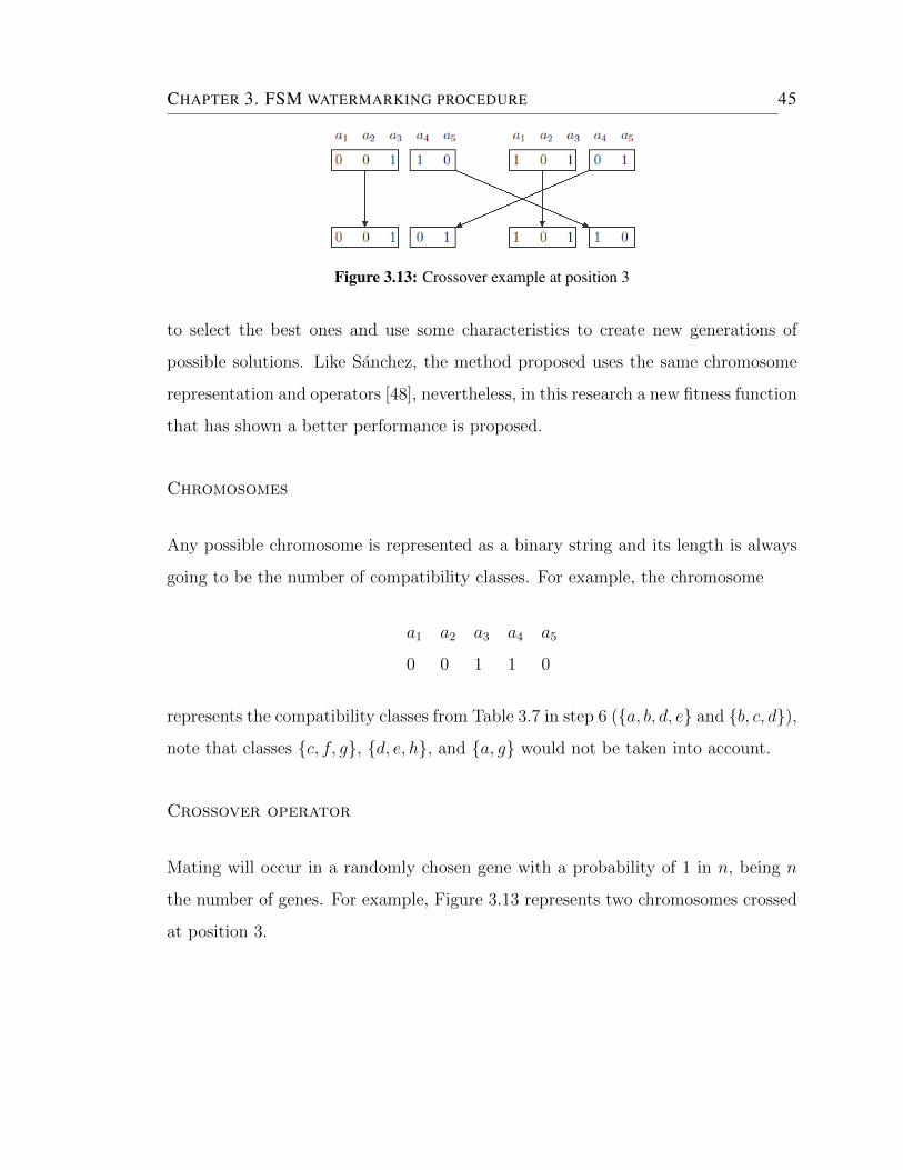
Crossover operator
Mating will occur in a randomly chosen gene with a probability of 1 in n, being n
the number of genes. For example, Figure 3.13 represents two chromosomes crossed
at position 3.
CHAPTER 3. FSM WATERMARKING PROCEDURE 46
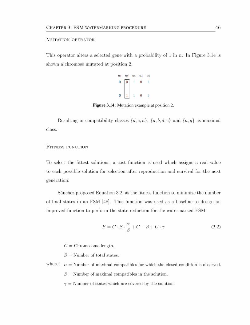
Mutation operator
This operator alters a selected gene with a probability of 1 in n. In Figure 3.14 is
shown a chromose mutated at position 2.
Figure 3.14: Mutation example at position 2.
Resulting in compatibility classes {d, e, h}, {a, b, d, e} and {a, g} as maximal
class.
Fitness function
To select the fittest solutions, a cost function is used which assigns a real value
to each possible solution for selection after reproduction and survival for the next
generation.
Sanchez proposed Equation 3.2, as the fitness function to minimize the number
of final states in an FSM [48]. This function was used as a baseline to design an
improved function to perform the state-reduction for the watermarked FSM.
F = C · S · αβ
+ C − β + C · γ (3.2)
where:
C = Chromosome length.
S = Number of total states.
α = Number of maximal compatibles for which the closed condition is observed.
β = Number of maximal compatibles in the solution.
γ = Number of states which are covered by the solution.
CHAPTER 3. FSM WATERMARKING PROCEDURE 47
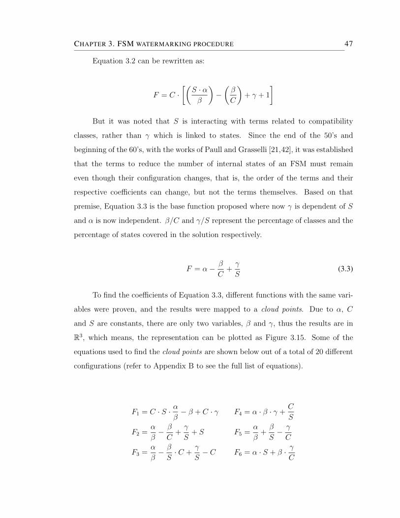
Equation 3.2 can be rewritten as:
F = C ·[(
S · αβ
)−(β
C
)+ γ + 1
]
But it was noted that S is interacting with terms related to compatibility
classes, rather than γ which is linked to states. Since the end of the 50’s and
beginning of the 60’s, with the works of Paull and Grasselli [21,42], it was established
that the terms to reduce the number of internal states of an FSM must remain
even though their configuration changes, that is, the order of the terms and their
respective coefficients can change, but not the terms themselves. Based on that
premise, Equation 3.3 is the base function proposed where now γ is dependent of S
and α is now independent. β/C and γ/S represent the percentage of classes and the
percentage of states covered in the solution respectively.
F = α− β
C+γ
S(3.3)
To find the coefficients of Equation 3.3, different functions with the same vari-
ables were proven, and the results were mapped to a cloud points. Due to α, C
and S are constants, there are only two variables, β and γ, thus the results are in
R3, which means, the representation can be plotted as Figure 3.15. Some of the
equations used to find the cloud points are shown below out of a total of 20 different
configurations (refer to Appendix B to see the full list of equations).
F1 = C · S · αβ− β + C · γ F4 = α · β · γ +
C
S
F2 =α
β− β
C+γ
S+ S F5 =
α
β+β
S− γ
C
F3 =α
β− β
S· C +
γ
S− C F6 = α · S + β · γ
C
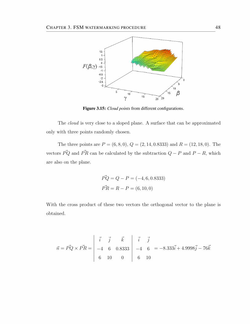
CHAPTER 3. FSM WATERMARKING PROCEDURE 48
Figure 3.15: Cloud points from different configurations.
The cloud is very close to a sloped plane. A surface that can be approximated
only with three points randomly chosen.
The three points are P = (6, 8, 0), Q = (2, 14, 0.8333) and R = (12, 18, 0). The
vectors ~PQ and ~PR can be calculated by the subtraction Q− P and P −R, which
are also on the plane.
~PQ = Q− P = (−4, 6, 0.8333)
~PR = R− P = (6, 10, 0)
With the cross product of these two vectors the orthogonal vector to the plane is
obtained.
~n = ~PQ× ~PR =
∣∣∣∣∣∣∣∣∣~i ~j ~k
−4 6 0.8333
6 10 0
∣∣∣∣∣∣∣∣∣~i ~j
−4 6
6 10
= −8.333~i+ 4.9998~j − 76~k
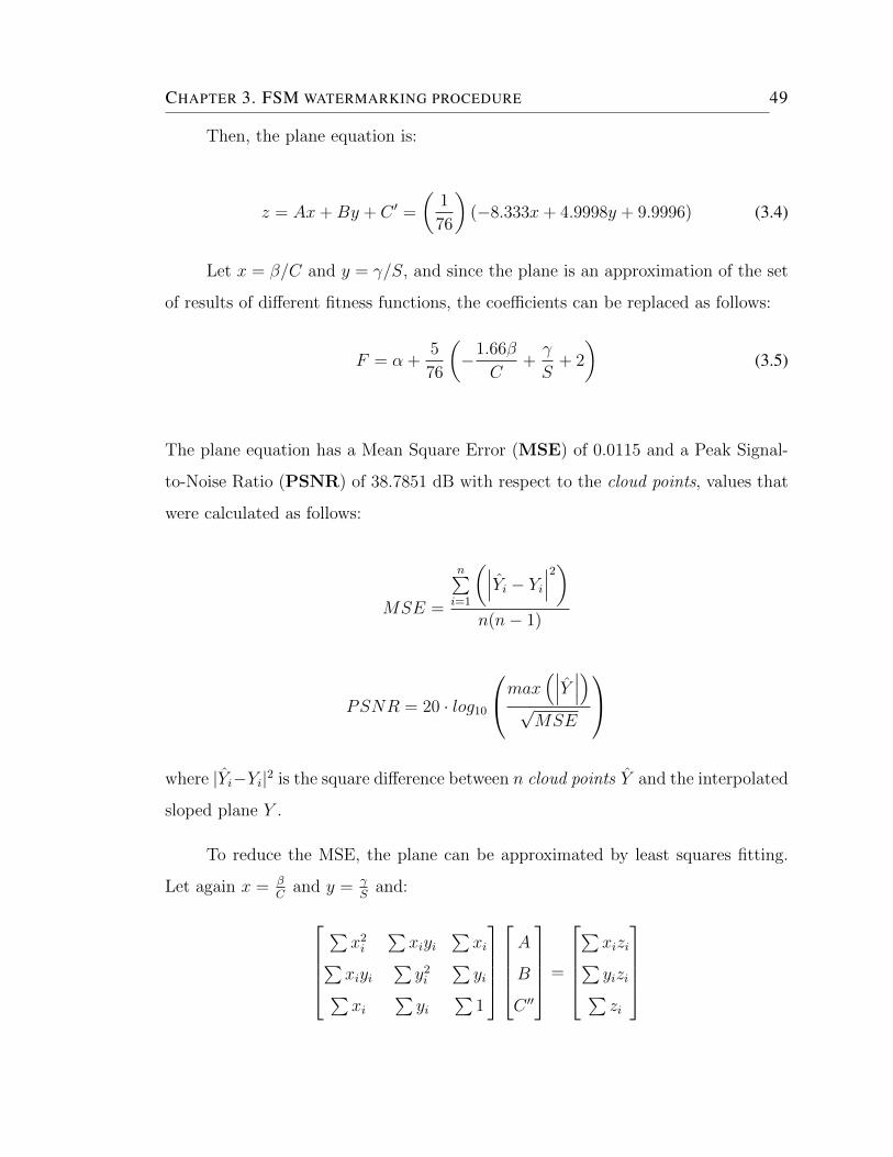
CHAPTER 3. FSM WATERMARKING PROCEDURE 49
Then, the plane equation is:
z = Ax+By + C ′ =
(1
76
)(−8.333x+ 4.9998y + 9.9996) (3.4)
Let x = β/C and y = γ/S, and since the plane is an approximation of the set
of results of different fitness functions, the coefficients can be replaced as follows:
F = α +5
76
(−1.66β
C+γ
S+ 2
)(3.5)
The plane equation has a Mean Square Error (MSE) of 0.0115 and a Peak Signal-
to-Noise Ratio (PSNR) of 38.7851 dB with respect to the cloud points, values that
were calculated as follows:
MSE =
n∑i=1
(∣∣∣Yi − Yi∣∣∣2)n(n− 1)
PSNR = 20 · log10
max(∣∣∣Y ∣∣∣)
√MSE
where |Yi−Yi|2 is the square difference between n cloud points Y and the interpolated
sloped plane Y .
To reduce the MSE, the plane can be approximated by least squares fitting.
Let again x = βC
and y = γS
and:
∑x2i
∑xiyi
∑xi∑
xiyi∑y2i
∑yi∑
xi∑yi
∑1
A
B
C ′′
=
∑xizi∑yizi∑zi
CHAPTER 3. FSM WATERMARKING PROCEDURE 50
which is equal to:10711.44165 21071.35575 1816.07197
21071.35575 47053.38285 4001.177778
1816.07197 4001.177778 568
A
B
C ′′
=
451.8089598
1254.968944
145.6158735
Then, A = −0.0898, B = 0.0516 and C ′′ = 0.1804, letting to:
F ′ = α− 0.0898β
C+ 0.0516
γ
S+ 0.1804 (3.6)
which is now closer to each point in the cloud points with a MSE of 0.0113 and a
PSNR of 38.9049 dB, which with the first approximation give differences of around
2× 10⁻⁴ and 0.1198 respectively.
However, the terms of any of both plane equations can be used to replace the
terms of the fitness function. This is possible because the aim of this approach is
to adjust the results space, allowing to reduce the noise, thus, optimal solutions are
more likely to be found, instead of being scattered through all the searching space.
Figure 3.16: Plane interpolation from the cloud points.
When the algorithm reaches the stop condition (minimum cost value returned
or number of generations), the chromosome with minimal cost value found will in-
dicate the compatibility classes to take into account and thus the remaining states
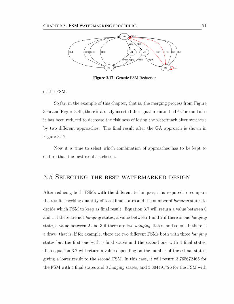
CHAPTER 3. FSM WATERMARKING PROCEDURE 51
Figure 3.17: Genetic FSM Reduction
of the FSM.
So far, in the example of this chapter, that is, the merging process from Figure
3.4a and Figure 3.4b, there is already inserted the signature into the IP Core and also
it has been reduced to decrease the riskiness of losing the watermark after synthesis
by two different approaches. The final result after the GA approach is shown in
Figure 3.17.
Now it is time to select which combination of approaches has to be kept to
endure that the best result is chosen.
3.5 Selecting the best watermarked design
After reducing both FSMs with the different techniques, it is required to compare
the results checking quantity of total final states and the number of hanging states to
decide which FSM to keep as final result. Equation 3.7 will return a value between 0
and 1 if there are not hanging states, a value between 1 and 2 if there is one hanging
state, a value between 2 and 3 if there are two hanging states, and so on. If there is
a draw, that is, if for example, there are two different FSMs both with three hanging
states but the first one with 5 final states and the second one with 4 final states,
then equation 3.7 will return a value depending on the number of these final states,
giving a lower result to the second FSM. In this case, it will return 3.765672465 for
the FSM with 4 final states and 3 hanging states, and 3.804491726 for the FSM with
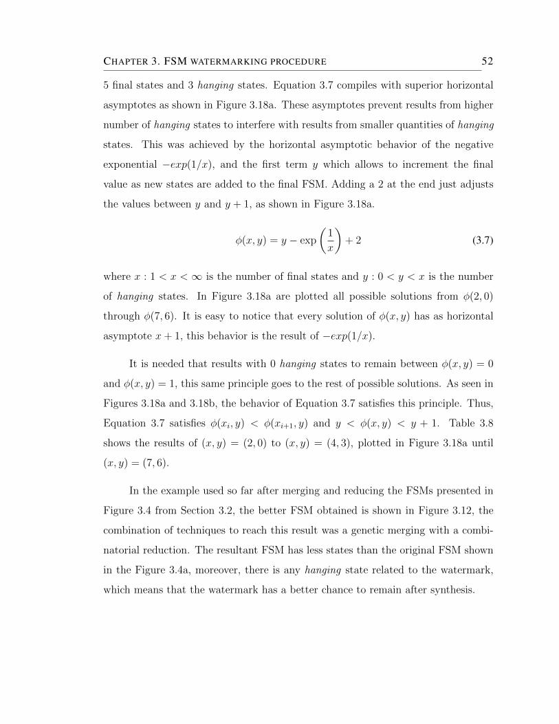
CHAPTER 3. FSM WATERMARKING PROCEDURE 52
5 final states and 3 hanging states. Equation 3.7 compiles with superior horizontal
asymptotes as shown in Figure 3.18a. These asymptotes prevent results from higher
number of hanging states to interfere with results from smaller quantities of hanging
states. This was achieved by the horizontal asymptotic behavior of the negative
exponential −exp(1/x), and the first term y which allows to increment the final
value as new states are added to the final FSM. Adding a 2 at the end just adjusts
the values between y and y + 1, as shown in Figure 3.18a.
φ(x, y) = y − exp
(1
x
)+ 2 (3.7)
where x : 1 < x < ∞ is the number of final states and y : 0 < y < x is the number
of hanging states. In Figure 3.18a are plotted all possible solutions from φ(2, 0)
through φ(7, 6). It is easy to notice that every solution of φ(x, y) has as horizontal
asymptote x+ 1, this behavior is the result of −exp(1/x).
It is needed that results with 0 hanging states to remain between φ(x, y) = 0
and φ(x, y) = 1, this same principle goes to the rest of possible solutions. As seen in
Figures 3.18a and 3.18b, the behavior of Equation 3.7 satisfies this principle. Thus,
Equation 3.7 satisfies φ(xi, y) < φ(xi+1, y) and y < φ(x, y) < y + 1. Table 3.8
shows the results of (x, y) = (2, 0) to (x, y) = (4, 3), plotted in Figure 3.18a until
(x, y) = (7, 6).
In the example used so far after merging and reducing the FSMs presented in
Figure 3.4 from Section 3.2, the better FSM obtained is shown in Figure 3.12, the
combination of techniques to reach this result was a genetic merging with a combi-
natorial reduction. The resultant FSM has less states than the original FSM shown
in the Figure 3.4a, moreover, there is any hanging state related to the watermark,
which means that the watermark has a better chance to remain after synthesis.
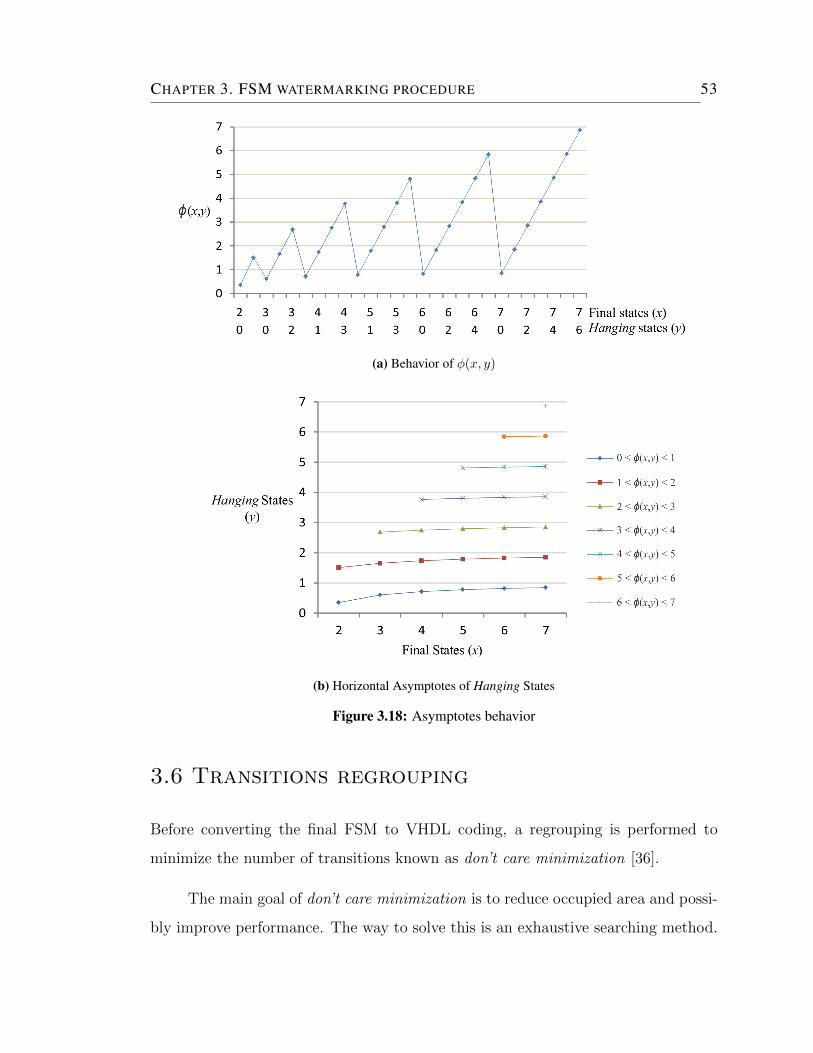
CHAPTER 3. FSM WATERMARKING PROCEDURE 53
(a) Behavior of φ(x, y)
(b) Horizontal Asymptotes of Hanging States
Figure 3.18: Asymptotes behavior
3.6 Transitions regrouping
Before converting the final FSM to VHDL coding, a regrouping is performed to
minimize the number of transitions known as don’t care minimization [36].
The main goal of don’t care minimization is to reduce occupied area and possi-
bly improve performance. The way to solve this is an exhaustive searching method.
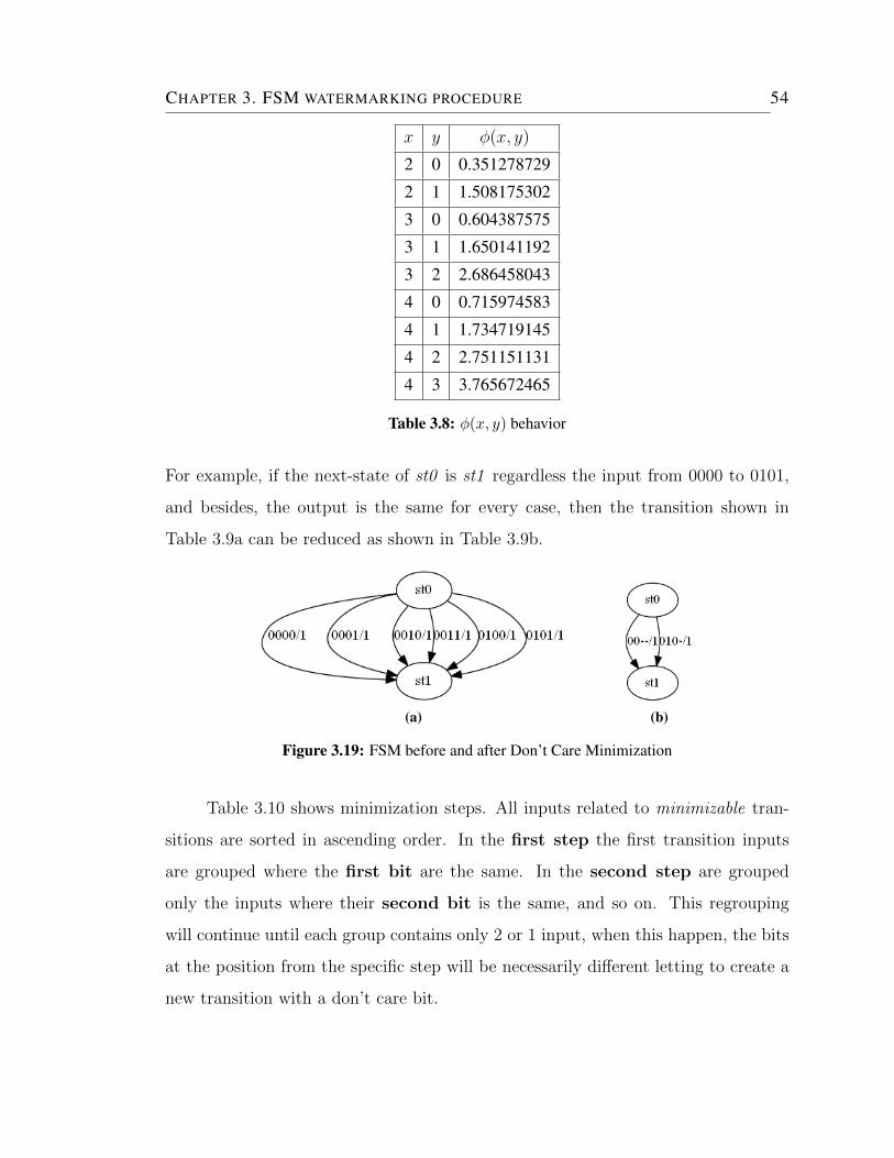
CHAPTER 3. FSM WATERMARKING PROCEDURE 54
x y φ(x, y)
2 0 0.351278729
2 1 1.508175302
3 0 0.604387575
3 1 1.650141192
3 2 2.686458043
4 0 0.715974583
4 1 1.734719145
4 2 2.751151131
4 3 3.765672465
Table 3.8: φ(x, y) behavior
For example, if the next-state of st0 is st1 regardless the input from 0000 to 0101,
and besides, the output is the same for every case, then the transition shown in
Table 3.9a can be reduced as shown in Table 3.9b.
(a) (b)
Figure 3.19: FSM before and after Don’t Care Minimization
Table 3.10 shows minimization steps. All inputs related to minimizable tran-
sitions are sorted in ascending order. In the first step the first transition inputs
are grouped where the first bit are the same. In the second step are grouped
only the inputs where their second bit is the same, and so on. This regrouping
will continue until each group contains only 2 or 1 input, when this happen, the bits
at the position from the specific step will be necessarily different letting to create a
new transition with a don’t care bit.
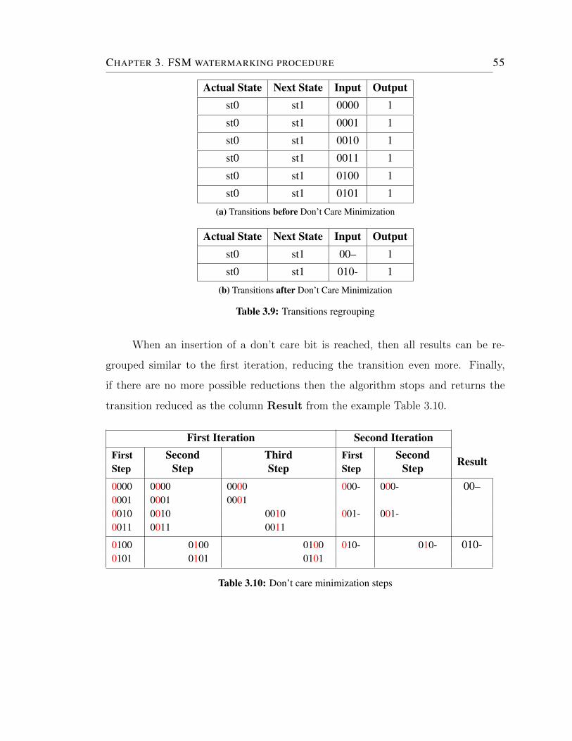
CHAPTER 3. FSM WATERMARKING PROCEDURE 55
Actual State Next State Input Outputst0 st1 0000 1
st0 st1 0001 1
st0 st1 0010 1
st0 st1 0011 1
st0 st1 0100 1
st0 st1 0101 1
(a) Transitions before Don’t Care Minimization
Actual State Next State Input Outputst0 st1 00– 1
st0 st1 010- 1
(b) Transitions after Don’t Care Minimization
Table 3.9: Transitions regrouping
When an insertion of a don’t care bit is reached, then all results can be re-
grouped similar to the first iteration, reducing the transition even more. Finally,
if there are no more possible reductions then the algorithm stops and returns the
transition reduced as the column Result from the example Table 3.10.
First Iteration Second IterationFirst Second Third First Second ResultStep Step Step Step Step0000 0000 0000 000- 000- 00–0001 0001 00010010 0010 0010 001- 001-0011 0011 0011
0100 0100 0100 010- 010- 010-0101 0101 0101
Table 3.10: Don’t care minimization steps
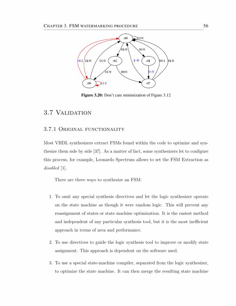
CHAPTER 3. FSM WATERMARKING PROCEDURE 56
Figure 3.20: Don’t care minimization of Figure 3.12
3.7 Validation
3.7.1 Original functionality
Most VHDL synthesizers extract FSMs found within the code to optimize and syn-
thesize them side by side [37]. As a matter of fact, some synthesizers let to configure
this process, for example, Leonardo Spectrum allows to set the FSM Extraction as
disabled [1].
There are three ways to synthesize an FSM:
1. To omit any special synthesis directives and let the logic synthesizer operate
on the state machine as though it were random logic. This will prevent any
reassignment of states or state machine optimization. It is the easiest method
and independent of any particular synthesis tool, but it is the most inefficient
approach in terms of area and performance.
2. To use directives to guide the logic synthesis tool to improve or modify state
assignment. This approach is dependent on the software used.
3. To use a special state-machine compiler, separated from the logic synthesizer,
to optimize the state machine. It can then merge the resulting state machine
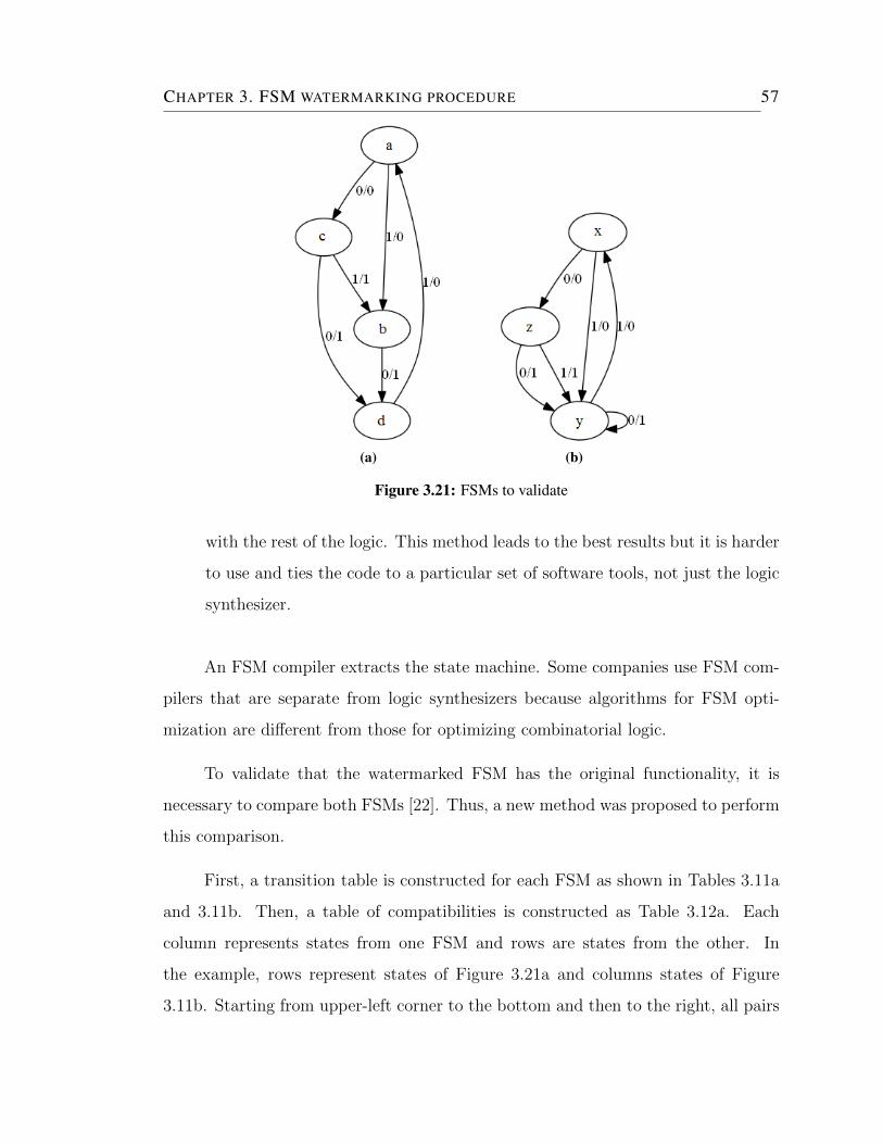
CHAPTER 3. FSM WATERMARKING PROCEDURE 57
(a) (b)
Figure 3.21: FSMs to validate
with the rest of the logic. This method leads to the best results but it is harder
to use and ties the code to a particular set of software tools, not just the logic
synthesizer.
An FSM compiler extracts the state machine. Some companies use FSM com-
pilers that are separate from logic synthesizers because algorithms for FSM opti-
mization are different from those for optimizing combinatorial logic.
To validate that the watermarked FSM has the original functionality, it is
necessary to compare both FSMs [22]. Thus, a new method was proposed to perform
this comparison.
First, a transition table is constructed for each FSM as shown in Tables 3.11a
and 3.11b. Then, a table of compatibilities is constructed as Table 3.12a. Each
column represents states from one FSM and rows are states from the other. In
the example, rows represent states of Figure 3.21a and columns states of Figure
3.11b. Starting from upper-left corner to the bottom and then to the right, all pairs
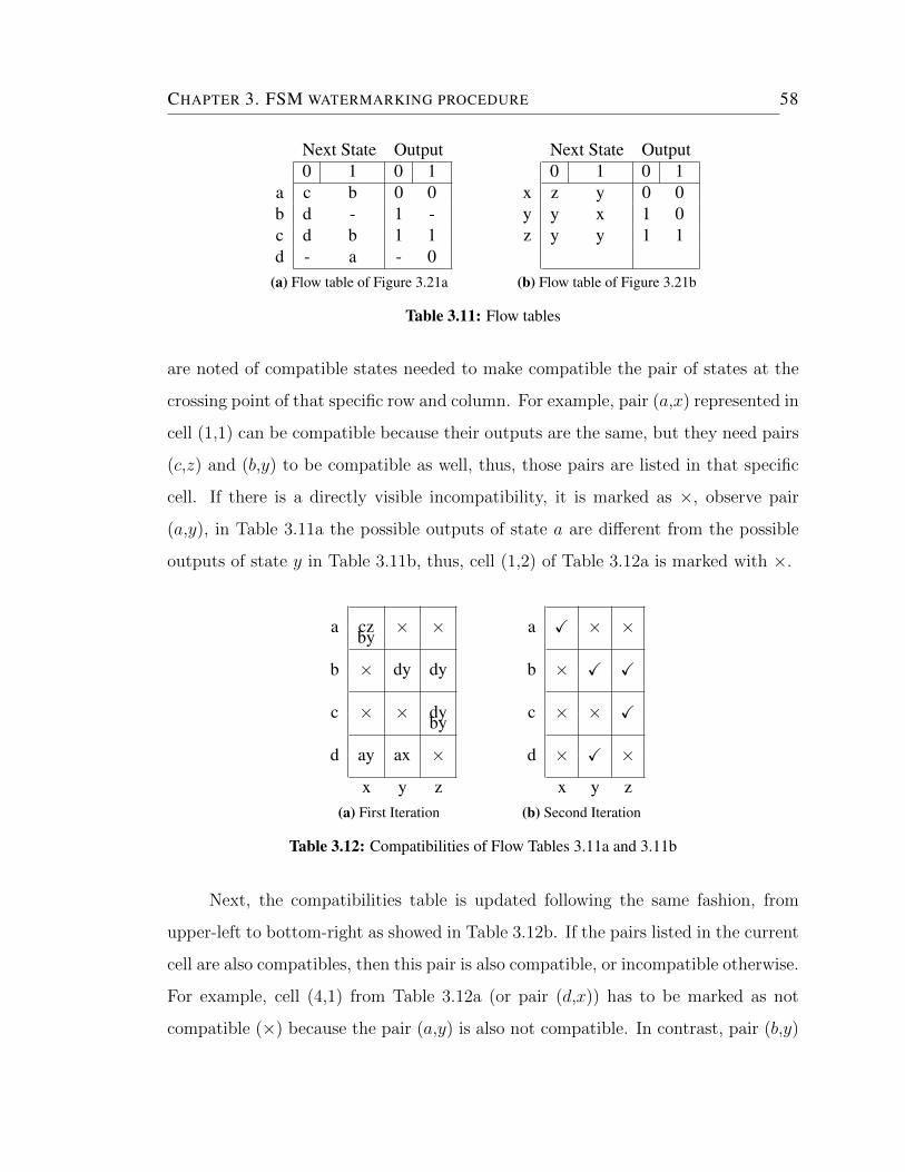
CHAPTER 3. FSM WATERMARKING PROCEDURE 58
Next State Output0 1 0 1
a c b 0 0b d - 1 -c d b 1 1d - a - 0
(a) Flow table of Figure 3.21a
Next State Output0 1 0 1
x z y 0 0y y x 1 0z y y 1 1
(b) Flow table of Figure 3.21b
Table 3.11: Flow tables
are noted of compatible states needed to make compatible the pair of states at the
crossing point of that specific row and column. For example, pair (a,x) represented in
cell (1,1) can be compatible because their outputs are the same, but they need pairs
(c,z) and (b,y) to be compatible as well, thus, those pairs are listed in that specific
cell. If there is a directly visible incompatibility, it is marked as ×, observe pair
(a,y), in Table 3.11a the possible outputs of state a are different from the possible
outputs of state y in Table 3.11b, thus, cell (1,2) of Table 3.12a is marked with ×.
a cz × ×by
b × dy dy
c × × dyby
d ay ax ×
x y z(a) First Iteration
a X × ×
b × X X
c × × X
d × X ×
x y z(b) Second Iteration
Table 3.12: Compatibilities of Flow Tables 3.11a and 3.11b
Next, the compatibilities table is updated following the same fashion, from
upper-left to bottom-right as showed in Table 3.12b. If the pairs listed in the current
cell are also compatibles, then this pair is also compatible, or incompatible otherwise.
For example, cell (4,1) from Table 3.12a (or pair (d,x)) has to be marked as not
compatible (×) because the pair (a,y) is also not compatible. In contrast, pair (b,y)
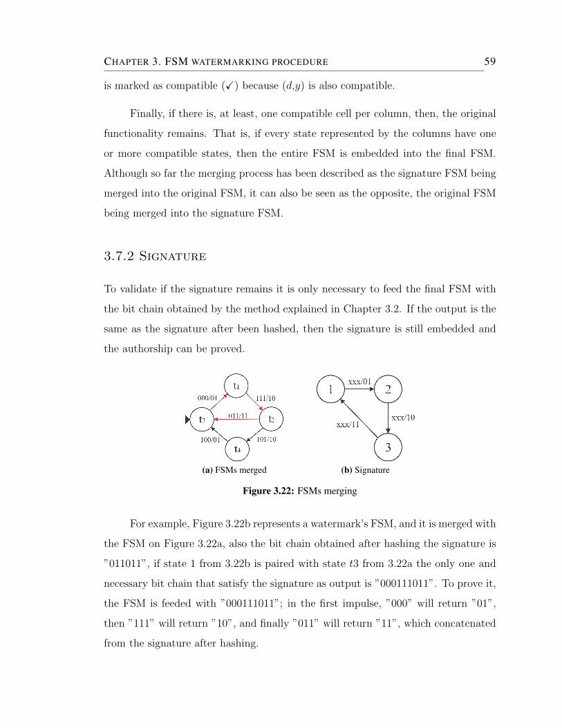
CHAPTER 3. FSM WATERMARKING PROCEDURE 59
is marked as compatible (X) because (d,y) is also compatible.
Finally, if there is, at least, one compatible cell per column, then, the original
functionality remains. That is, if every state represented by the columns have one
or more compatible states, then the entire FSM is embedded into the final FSM.
Although so far the merging process has been described as the signature FSM being
merged into the original FSM, it can also be seen as the opposite, the original FSM
being merged into the signature FSM.
3.7.2 Signature
To validate if the signature remains it is only necessary to feed the final FSM with
the bit chain obtained by the method explained in Chapter 3.2. If the output is the
same as the signature after been hashed, then the signature is still embedded and
the authorship can be proved.
(a) FSMs merged (b) Signature
Figure 3.22: FSMs merging
For example, Figure 3.22b represents a watermark’s FSM, and it is merged with
the FSM on Figure 3.22a, also the bit chain obtained after hashing the signature is
”011011”, if state 1 from 3.22b is paired with state t3 from 3.22a the only one and
necessary bit chain that satisfy the signature as output is ”000111011”. To prove it,
the FSM is feeded with ”000111011”; in the first impulse, ”000” will return ”01”,
then ”111” will return ”10”, and finally ”011” will return ”11”, which concatenated
from the signature after hashing.
Chapter 4
Experimental results analysis
4.1 Experimental setup
All comparisons and experiments were made using Finite State Machines (FSMs)
from ACM/SIGDA benchmarks library [11], specially LGSynth series (High-Level
Synthesis Workshops) from Collaborative Benchmarking and Experimental Algorith-
mics Laboratory granted by the Design, Verification and Test Division of Mentor
Graphics Corporation.
The experimentation were carried out with double precision. The machine used
in every experiment has a machine epsilon in double precision of 2−53 with a mini-
mum positive value in double precision of 4.94065645841247E-324. The processor is
an Intel Core 2 Duo with a clock velocity of 1.5 GHz. The Operating System (OS)
is Windows 7 of 32 bits with 3.00 GB of RAM memory available. The codification
was written in C# 5.0 in .NET 4.5 using Visual Studio 2012.
The Genetic Algorithms (GAs) configuration used during experimentation is
described below.
60
CHAPTER 4. EXPERIMENTAL RESULTS ANALYSIS 61
4.1.1 Random seeds
New population of chromosomes are specified by 50 percent of probability by each
gene. It was used the pseudo-random method of C# to obtain values between 0.0
and 0.99999999999999978 seeded from the system clock. If this pseudo-random value
is greater than 0.5 then the gene is equal to 1, otherwise it is set to 0. Mutation and
mating positions are set by the same pseudo-random method.
4.1.2 GA specifics for merging
Binary representation has been used to represent the number of states, therefore the
chromosome length is n ·m bits, where:
n = number of states in the FSM signature,
m = number of states in the RTL’s FSM.
An initial population is defined by P individuals or solutions.
P = r!−r−1∑i=1
i! with r = max(m,n) (4.1)
Crossover operation works by exchanging genetic material between solutions,
for example, an individual 010001100000 recombining at 2nd crossover position with
individual 000001000100 results in offspring 010001000100 (node 2 matches node t1,
node 3 matches node t2, node t4 has no match, etc) and 000001100000 (node t1 has
no match, node 3 matches node t2, node 1 matches node t3, etc).
During mutation, it is necessary to check if a mutated offspring does not result
in an invalid chromosome. This can be done by verifying that a chromosome package
has only one-hot, for example, packages like 011 are considered invalid; moreover,
a chromosome could represent a maximum of n one-hot genes. For example, if the
chromosome 010001100000 is mutated at gene 2, the new chromosome would be
CHAPTER 4. EXPERIMENTAL RESULTS ANALYSIS 62
000001100000.
4.1.3 GA specifics for reduction
Any possible solution is expressed in binary form representing a combination of
compatibility classes and its length is the total of those classes. There are 2C indi-
viduals in the initial population with C being the number of compatibility classes.
For mating, individuals exchange genetic material according to crossover probability
at a random position. For example, chromosomes 00110 and 10101 recombined at
position 3 would generate offspring 00101 and 10110. After, children are mutated by
flipping genes according to mutation’s probability, for example, chromosome 00101
mutated at position 2 would create chromosome 01101 resulting in compatibility
classes C2, C3 and C5 as maximal classes. The function on Equation 4.2 was used
as objective function.
F = α +5
76
(−1.66β
C+γ
S+ 2
)(4.2)
4.2 Reported results
The proposed method aims to insert information in FSM transitions, yet, reported
results also show the number of states, transitions and bits that have been reduced.
As mentioned above, all results shown here were taken from the LGSynth
benchmark library and compared with the best results found in literature. The
proposals that were chosen to be compare with, are focused in FSM reduction, aimed
to emphasize the final number of states, particularly of hanging states; and FSM
watermarking to compare the number of final transitions, final states and number
of bits embedded.
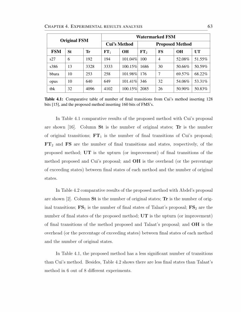
CHAPTER 4. EXPERIMENTAL RESULTS ANALYSIS 63
Original FSMWatermarked FSM
Cui’s Method Proposed MethodFSM St Tr FT1 OH FT2 FS OH UT
s27 6 192 194 101.04% 100 4 52.08% 51.55%
s386 13 3328 3333 100.15% 1686 30 50.66% 50.59%
bbara 10 253 258 101.98% 176 7 69.57% 68.22%
opus 10 640 649 101.41% 346 32 54.06% 53.31%
tbk 32 4096 4102 100.15% 2085 26 50.90% 50.83%
Table 4.1: Comparative table of number of final transitions from Cui’s method inserting 128bits [15], and the proposed method inserting 160 bits of FMS’s.
In Table 4.1 comparative results of the proposed method with Cui’s proposal
are shown [16]. Column St is the number of original states; Tr is the number
of original transitions; FT1 is the number of final transitions of Cui’s proposal;
FT2 and FS are the number of final transitions and states, respectively, of the
proposed method; UT is the upturn (or improvement) of final transitions of the
method proposed and Cui’s proposal; and OH is the overhead (or the percentage
of exceeding states) between final states of each method and the number of original
states.
In Table 4.2 comparative results of the proposed method with Abdel’s proposal
are shown [2]. Column St is the number of original states; Tr is the number of orig-
inal transitions; FS1 is the number of final states of Talaat’s proposal; FS2 are the
number of final states of the proposed method; UT is the upturn (or improvement)
of final transitions of the method proposed and Talaat’s proposal; and OH is the
overhead (or the percentage of exceeding states) between final states of each method
and the number of original states.
In Table 4.1, the proposed method has a less significant number of transitions
than Cui’s method. Besides, Table 4.2 shows there are less final states than Talaat’s
method in 6 out of 8 different experiments.
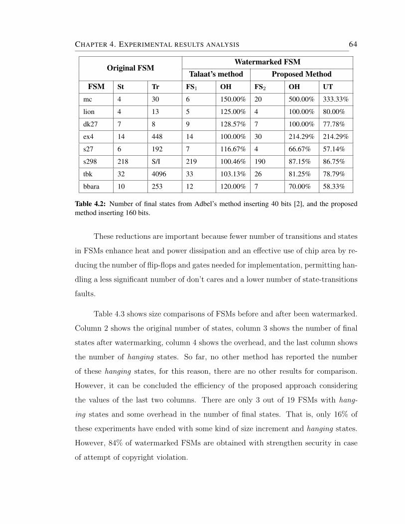
CHAPTER 4. EXPERIMENTAL RESULTS ANALYSIS 64
Original FSMWatermarked FSM
Talaat’s method Proposed MethodFSM St Tr FS1 OH FS2 OH UT
mc 4 30 6 150.00% 20 500.00% 333.33%
lion 4 13 5 125.00% 4 100.00% 80.00%
dk27 7 8 9 128.57% 7 100.00% 77.78%
ex4 14 448 14 100.00% 30 214.29% 214.29%
s27 6 192 7 116.67% 4 66.67% 57.14%
s298 218 S/I 219 100.46% 190 87.15% 86.75%
tbk 32 4096 33 103.13% 26 81.25% 78.79%
bbara 10 253 12 120.00% 7 70.00% 58.33%
Table 4.2: Number of final states from Adbel’s method inserting 40 bits [2], and the proposedmethod inserting 160 bits.
These reductions are important because fewer number of transitions and states
in FSMs enhance heat and power dissipation and an effective use of chip area by re-
ducing the number of flip-flops and gates needed for implementation, permitting han-
dling a less significant number of don’t cares and a lower number of state-transitions
faults.
Table 4.3 shows size comparisons of FSMs before and after been watermarked.
Column 2 shows the original number of states, column 3 shows the number of final
states after watermarking, column 4 shows the overhead, and the last column shows
the number of hanging states. So far, no other method has reported the number
of these hanging states, for this reason, there are no other results for comparison.
However, it can be concluded the efficiency of the proposed approach considering
the values of the last two columns. There are only 3 out of 19 FSMs with hang-
ing states and some overhead in the number of final states. That is, only 16% of
these experiments have ended with some kind of size increment and hanging states.
However, 84% of watermarked FSMs are obtained with strengthen security in case
of attempt of copyright violation.
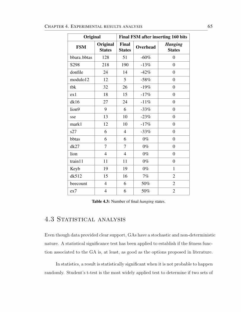
CHAPTER 4. EXPERIMENTAL RESULTS ANALYSIS 65
Original Final FSM after inserting 160 bits
FSM Original Final Overhead HangingStates States States
bbara bbtas 128 51 -60% 0
S298 218 190 -13% 0
donfile 24 14 -42% 0
modulo12 12 5 -58% 0
tbk 32 26 -19% 0
ex1 18 15 -17% 0
dk16 27 24 -11% 0
lion9 9 6 -33% 0
sse 13 10 -23% 0
mark1 12 10 -17% 0
s27 6 4 -33% 0
bbtas 6 6 0% 0
dk27 7 7 0% 0
lion 4 4 0% 0
train11 11 11 0% 0
Keyb 19 19 0% 1
dk512 15 16 7% 2
beecount 4 6 50% 2
ex7 4 6 50% 2
Table 4.3: Number of final hanging states.
4.3 Statistical analysis
Even though data provided clear support, GAs have a stochastic and non-deterministic
nature. A statistical significance test has been applied to establish if the fitness func-
tion associated to the GA is, at least, as good as the options proposed in literature.
In statistics, a result is statistically significant when it is not probable to happen
randomly. Student’s t-test is the most widely applied test to determine if two sets of
CHAPTER 4. EXPERIMENTAL RESULTS ANALYSIS 66
data are significantly different from each other [49], nevertheless, it needs the data
to follow a normal distribution.
There are tests to avoid normal distribution, or nonparametric statistical tests
like Wilcoxon signed-rank test [53].
4.3.1 Wilcoxon signed-rank test
It has been proven by non-parametric statistical hypothesis Wilcoxon signed-rank
test that experimental results shown in Tables 4.4 and 4.5 has statistically signifi-
cant difference when comparing base function in Equation 4.3 with final function in
Equation 4.4. Finally, final function in Equation in 4.4 was compared with Equation
3.2 proposed by Sanchez in [48].
F = α− β
C+γ
S(4.3)
F = α +5
76
(−1.66β
C+γ
S+ 2
)(4.4)
Table 4.4 shows experiments with FSMs after been watermarked, O column is the
number of original states, Fb is the number of states obtained after reduction with
base function in Equation 4.3, Ff is the number of states obtained after reduction
with final function in Equation 4.4, D is Fb-Ff difference and Index and Ranks
columns are inherited from Wilcoxon signed ranked test.
Ranks designated to indexes 1 to 5 are the same because the mean value is
equal to Equation 4.5.
(1
k
) k∑l=1
l =k + 1
2, if k = 5→ 5 + 1
2= 3 (4.5)
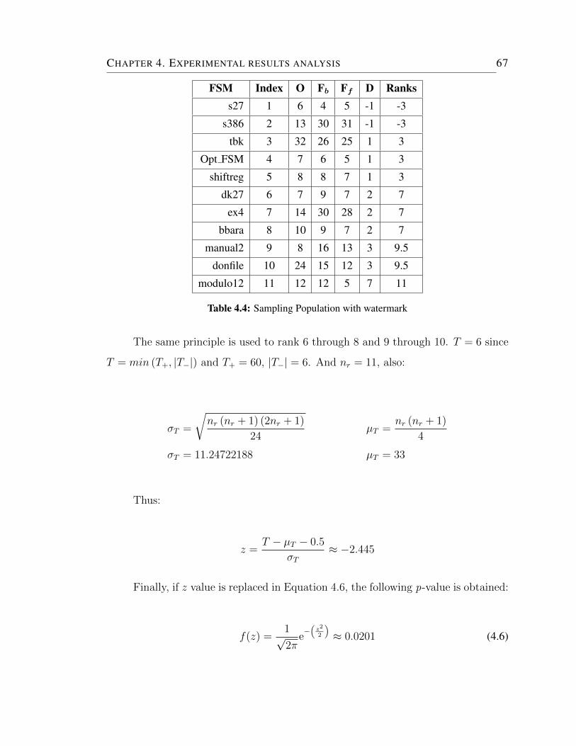
CHAPTER 4. EXPERIMENTAL RESULTS ANALYSIS 67
FSM Index O Fb Ff D Rankss27 1 6 4 5 -1 -3
s386 2 13 30 31 -1 -3
tbk 3 32 26 25 1 3
Opt FSM 4 7 6 5 1 3
shiftreg 5 8 8 7 1 3
dk27 6 7 9 7 2 7
ex4 7 14 30 28 2 7
bbara 8 10 9 7 2 7
manual2 9 8 16 13 3 9.5
donfile 10 24 15 12 3 9.5
modulo12 11 12 12 5 7 11
Table 4.4: Sampling Population with watermark
The same principle is used to rank 6 through 8 and 9 through 10. T = 6 since
T = min (T+, |T−|) and T+ = 60, |T−| = 6. And nr = 11, also:
σT =
√nr (nr + 1) (2nr + 1)
24µT =
nr (nr + 1)
4
σT = 11.24722188 µT = 33
Thus:
z =T − µT − 0.5
σT≈ −2.445
Finally, if z value is replaced in Equation 4.6, the following p-value is obtained:
f(z) =1√2π
e−(
z2
2
)≈ 0.0201 (4.6)
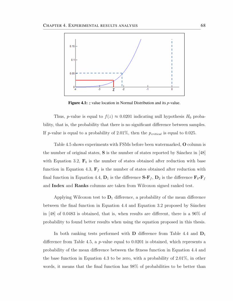
CHAPTER 4. EXPERIMENTAL RESULTS ANALYSIS 68
Figure 4.1: z value location in Normal Distribution and its p-value.
Thus, p-value is equal to f(z) ≈ 0.0201 indicating null hypothesis H0 proba-
bility, that is, the probability that there is no significant difference between samples.
If p-value is equal to a probability of 2.01%, then the pcritical is equal to 0.025.
Table 4.5 shows experiments with FSMs before been watermarked, O column is
the number of original states, S is the number of states reported by Sanchez in [48]
with Equation 3.2, Fb is the number of states obtained after reduction with base
function in Equation 4.3, Ff is the number of states obtained after reduction with
final function in Equation 4.4, D1 is the difference S-Ff , D2 is the difference Fb-Ff
and Index and Ranks columns are taken from Wilcoxon signed ranked test.
Applying Wilcoxon test to D1 difference, a probability of the mean difference
between the final function in Equation 4.4 and Equation 3.2 proposed by Sanchez
in [48] of 0.0483 is obtained, that is, when results are different, there is a 96% of
probability to found better results when using the equation proposed in this thesis.
In both ranking tests performed with D difference from Table 4.4 and D1
difference from Table 4.5, a p-value equal to 0.0201 is obtained, which represents a
probability of the mean difference between the fitness function in Equation 4.4 and
the base function in Equation 4.3 to be zero, with a probability of 2.01%, in other
words, it means that the final function has 98% of probabilities to be better than
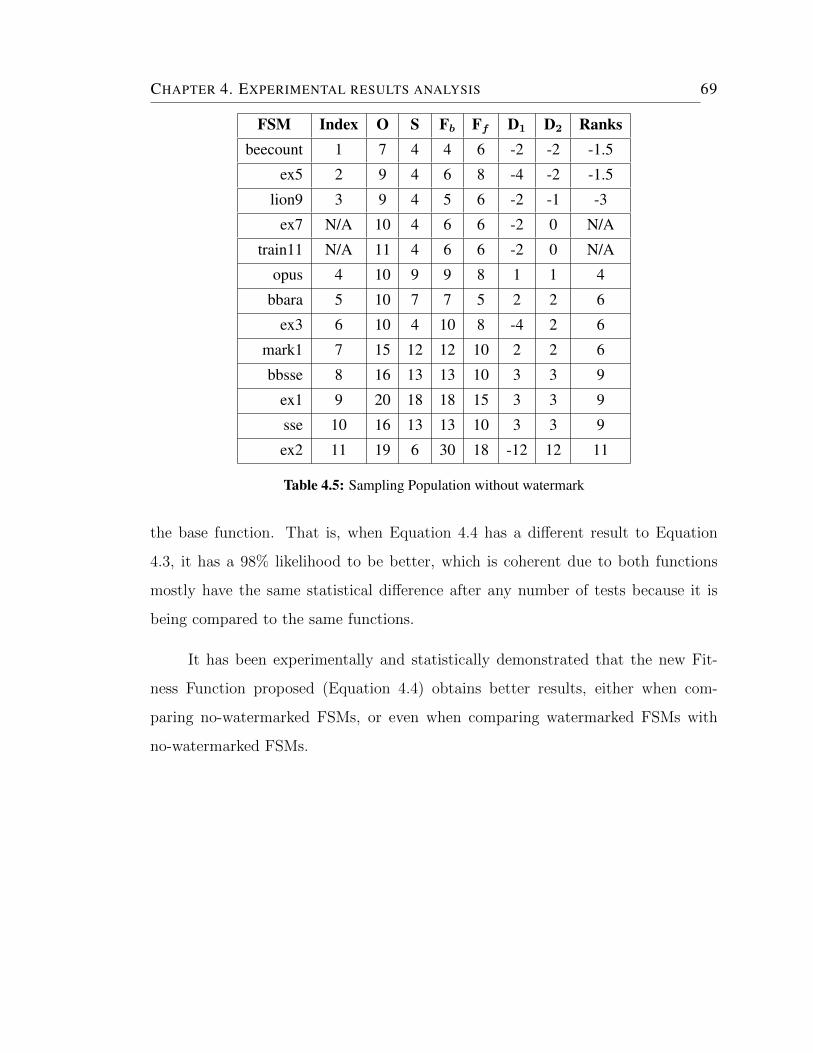
CHAPTER 4. EXPERIMENTAL RESULTS ANALYSIS 69
FSM Index O S Fb Ff D1 D2 Ranksbeecount 1 7 4 4 6 -2 -2 -1.5
ex5 2 9 4 6 8 -4 -2 -1.5
lion9 3 9 4 5 6 -2 -1 -3
ex7 N/A 10 4 6 6 -2 0 N/A
train11 N/A 11 4 6 6 -2 0 N/A
opus 4 10 9 9 8 1 1 4
bbara 5 10 7 7 5 2 2 6
ex3 6 10 4 10 8 -4 2 6
mark1 7 15 12 12 10 2 2 6
bbsse 8 16 13 13 10 3 3 9
ex1 9 20 18 18 15 3 3 9
sse 10 16 13 13 10 3 3 9
ex2 11 19 6 30 18 -12 12 11
Table 4.5: Sampling Population without watermark
the base function. That is, when Equation 4.4 has a different result to Equation
4.3, it has a 98% likelihood to be better, which is coherent due to both functions
mostly have the same statistical difference after any number of tests because it is
being compared to the same functions.
It has been experimentally and statistically demonstrated that the new Fit-
ness Function proposed (Equation 4.4) obtains better results, either when com-
paring no-watermarked FSMs, or even when comparing watermarked FSMs with
no-watermarked FSMs.
Chapter 5
Conclusions
Watermarking IP Cores by merging and state-reduction involving Finite State Ma-
chines using Genetic Algorithms leads to enhance heat and power dissipation and an
effective use of chip area, besides, it also permits handling a smaller number of don’t
cares, all of that with a more secure embedded signature which can be extracted
from any kind of file of any size. When found, even one FSM from HDL coding, is
guaranteed to watermark the IP Core and to recover the signature without original
functionality nor watermark disruption.
5.1 Remarks
This thesis presented a new approach to watermark IP Cores at a behavioral level
by merging and reducing Finite State Machines using Genetic and deterministic
algorithms. The proposed approach is based on previous proposals, achieving a
stronger signature, mainly due to the proposed post state-reduction method and its
new fitness function (see Equation 3.5 from Section 3.4.2).
This equation has been concluded after studying the behavior of several con-
figurations of fitness functions with the same variables and interpolating its charac-
teristic equation (see Section 3.4.2, equation 3.4). By doing this, it was possible to
reduce the space of satisfaction instead of scatter the solutions through all the search
70
CHAPTER 5. CONCLUSIONS 71
space. This conclusion aims to improve Finite State Machine merging by Genetic
Algorithms as future work.
The proposed method consists in extracting and translating HDL code and
some signature file into FSMs. Both FSMs are later merged and state-reduced by
Discrete Combinatorial and Standard Genetic Algorithms. It was presented Equa-
tion 3.7 from Section 3.5, aimed to select which combination of algorithms has
returned the best solution.
It also has been implemented a greedy post transitions-reduction based in a
don’t care approach and a VHDL translation from watermarked FSMs, as seen in
Section 3.6.
5.2 Future work
It has been deduced that hanging states are the true responsible of weak watermark-
ing and that reducing them to the minimum leads to a more secure signature. It also
has been experimentally proven that reducing watermarked Finite State Machines
does not imply to lose the original functionality neither its embedded signature.
It was also proven that Sanchez proposal is an efficient way to find possible com-
binations of prime classes to solve the post states-reduction [48]. It is considered
that their work deserves future research, being a new point of reference the fitness
function proposed in this thesis.
5.3 Contributions
In this thesis it has been shown that it is possible to obtain watermarked FSMs
with fewer states than an FSM without been watermarked. For example, difference
column D in Table 4.4, shows that the reduction method proposed achieved similar
CHAPTER 5. CONCLUSIONS 72
or better results, even tough the FSMs used have more information. Even more, in
almost every case, the final FSMs ends with fewer states than before watermarking.
To make this possible, a better fitness function has been proposed, showing better
performance to state-reduce FSMs.
A proposal to find the coefficients related to objective functions aimed to state
reduction as starting point by surface’s fitting has been also presented. Optimal
solutions are more likely to be found, instead of being scattered through all the
searching space.
Moreover, in addition to reporting differences tables, the number of hanging
states was also reported, a term defined in this thesis; and which to the best of the
knowledge, has never been done. This is important, due to starting from this work,
now it is possible to compare future with previous works concerning to FSM merging
and watermarking mainly aimed to watermark robustness.

Appendices
73
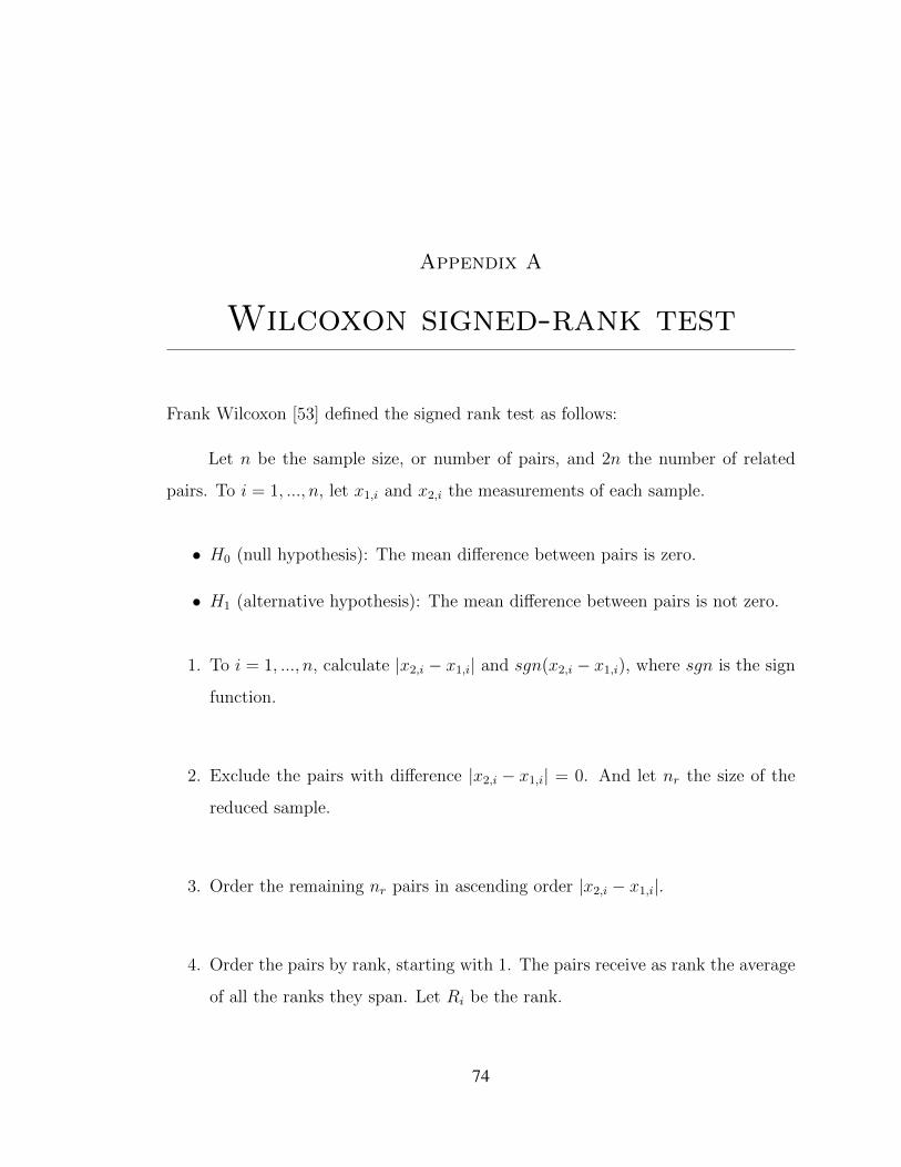
Appendix A
Wilcoxon signed-rank test
Frank Wilcoxon [53] defined the signed rank test as follows:
Let n be the sample size, or number of pairs, and 2n the number of related
pairs. To i = 1, ..., n, let x1,i and x2,i the measurements of each sample.
• H0 (null hypothesis): The mean difference between pairs is zero.
• H1 (alternative hypothesis): The mean difference between pairs is not zero.
1. To i = 1, ..., n, calculate |x2,i − x1,i| and sgn(x2,i − x1,i), where sgn is the sign
function.
2. Exclude the pairs with difference |x2,i − x1,i| = 0. And let nr the size of the
reduced sample.
3. Order the remaining nr pairs in ascending order |x2,i − x1,i|.
4. Order the pairs by rank, starting with 1. The pairs receive as rank the average
of all the ranks they span. Let Ri be the rank.
74
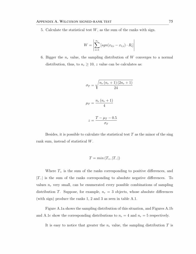
APPENDIX A. WILCOXON SIGNED-RANK TEST 75
5. Calculate the statistical test W , as the sum of the ranks with sign.
W =
∣∣∣∣∣nr∑i=1
[sgn(x2,i − x1,i) ·Ri]
∣∣∣∣∣6. Bigger the nr value, the sampling distribution of W converges to a normal
distribution, thus, to nr ≥ 10, z value can be calculates as:
σT =
√nr (nr + 1) (2nr + 1)
24
µT =nr (nr + 1)
4
z =T − µT − 0.5
σT
Besides, it is possible to calculate the statistical test T as the minor of the sing
rank sum, instead of statistical W .
T = min (T+, |T−|)
Where T+ is the sum of the ranks corresponding to positive differences, and
|T−| is the sum of the ranks corresponding to absolute negative differences. To
values nr very small, can be enumerated every possible combinations of sampling
distribution T . Suppose, for example, nr = 3 objects, whose absolute differences
(with sign) produce the ranks 1, 2 and 3 as seen in table A.1.
Figure A.1a shows the sampling distribution of this situation, and Figures A.1b
and A.1c show the corresponding distributions to nr = 4 and nr = 5 respectively.
It is easy to notice that greater the nr value, the sampling distribution T is
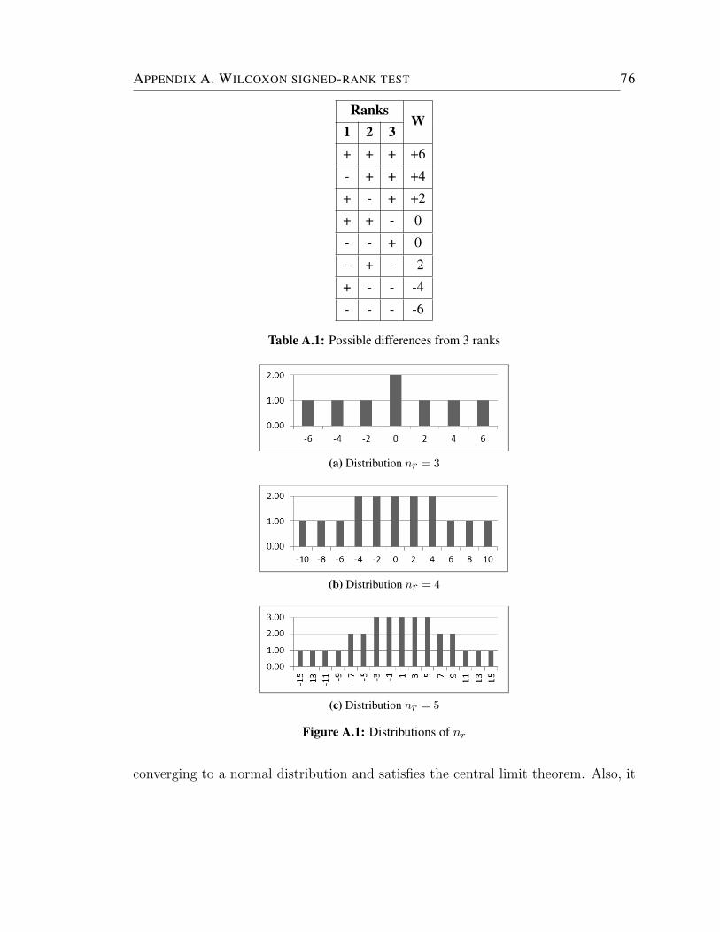
APPENDIX A. WILCOXON SIGNED-RANK TEST 76
RanksW
1 2 3+ + + +6
- + + +4
+ - + +2
+ + - 0
- - + 0
- + - -2
+ - - -4
- - - -6
Table A.1: Possible differences from 3 ranks
(a) Distribution nr = 3
(b) Distribution nr = 4
(c) Distribution nr = 5
Figure A.1: Distributions of nr
converging to a normal distribution and satisfies the central limit theorem. Also, it
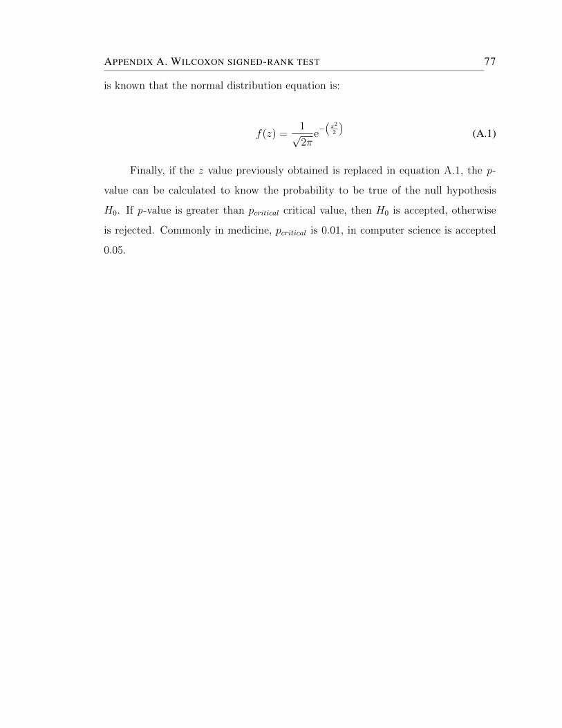
APPENDIX A. WILCOXON SIGNED-RANK TEST 77
is known that the normal distribution equation is:
f(z) =1√2π
e−(
z2
2
)(A.1)
Finally, if the z value previously obtained is replaced in equation A.1, the p-
value can be calculated to know the probability to be true of the null hypothesis
H0. If p-value is greater than pcritical critical value, then H0 is accepted, otherwise
is rejected. Commonly in medicine, pcritical is 0.01, in computer science is accepted
0.05.

Appendix B
List of equations
The 20 equations used to obtain the cloud points are listed below with their respec-
tive characteristic graphs, α, C and S were fixed to the same value for each different
graph. Due to that Genetic Algorithms (GA) are stochastic, each one of the equa-
tions was tested 5 times for each Finite State Machine (FSM). All the FSMs were
taken from LGSynth benchmarks.
In Figure B.1 the sum of all the equations listed below is presented. As seen
in Figure B.1, every equation has a similar behavior, except for F11 and F14 that
have values F (β, γ) up to 400. It was intended that the proposed equations span
their values throughout all the search space. However, when these equations are
bounded to values found during state-reduction for α, β, γ, C and S, they tend
to behave similarly. This similar behavior was the key to find the cloud points
presented in Figure 3.15 from Section 3.4.2. That is, even though their characteristic
graphs are not exactly like the mentioned cloud due to this graphs span the entire
surface by taking every possible F (β, γ) value, when they are evaluated with values
found during state-reduction, they create said cloud because now they are being
only evaluated in such values.
78
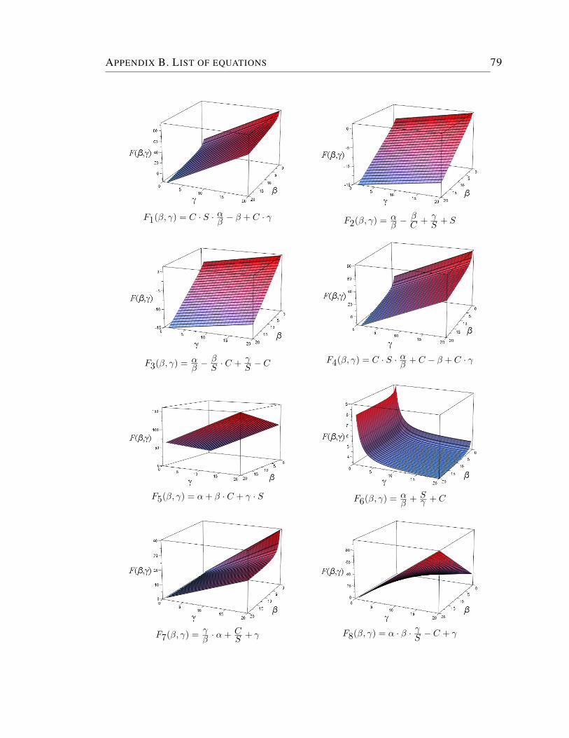
APPENDIX B. LIST OF EQUATIONS 79
F1(β, γ) = C · S · αβ− β + C · γ F2(β, γ) =
αβ− βC +
γS + S
F3(β, γ) =αβ− βS · C +
γS − C
F4(β, γ) = C · S · αβ+ C − β + C · γ
F5(β, γ) = α+ β · C + γ · S F6(β, γ) =αβ+ Sγ + C
F7(β, γ) =γβ· α+ C
S + γ F8(β, γ) = α · β · γS − C + γ
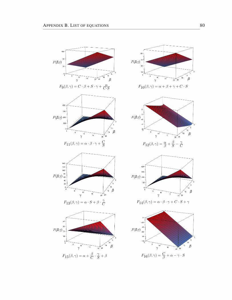
APPENDIX B. LIST OF EQUATIONS 80
F9(β, γ) = C · β + S · γ + αC·S F10(β, γ) = α+ β + γ + C · S
F11(β, γ) = α · β · γ + CS F12(β, γ) =
αβ+βS −
γC
F13(β, γ) = α · S + β · γC F14(β, γ) = α · β · γ + C · S + γ
F15(β, γ) = α+βC ·
γS + β F16(β, γ) =
Cβ
+ α− γ · S
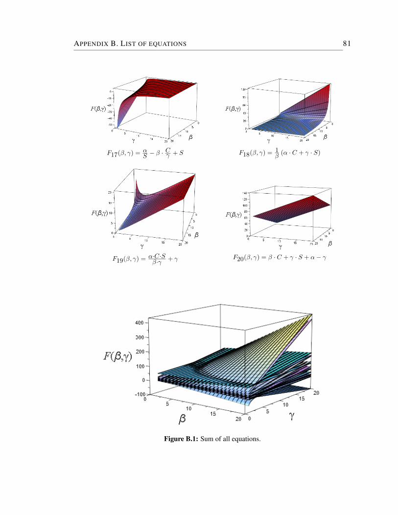
APPENDIX B. LIST OF EQUATIONS 81
F17(β, γ) =αS − β ·
Cγ + S F18(β, γ) =
1β(α · C + γ · S)
F19(β, γ) =α·C·Sβ·γ + γ F20(β, γ) = β · C + γ · S + α− γ
Figure B.1: Sum of all equations.
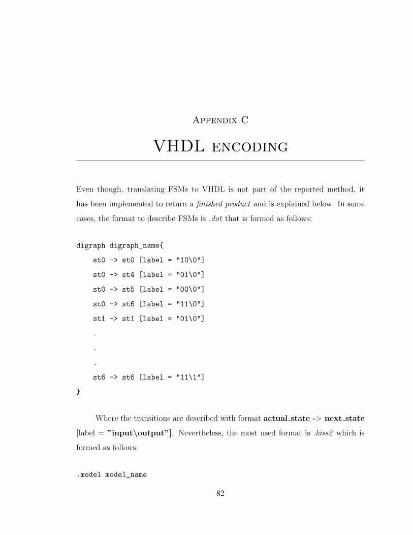
Appendix C
VHDL encoding
Even though, translating FSMs to VHDL is not part of the reported method, it
has been implemented to return a finished product and is explained below. In some
cases, the format to describe FSMs is .dot that is formed as follows:
digraph digraph_name{
st0 -> st0 [label = "10\0"]
st0 -> st4 [label = "01\0"]
st0 -> st5 [label = "00\0"]
st0 -> st6 [label = "11\0"]
st1 -> st1 [label = "01\0"]
.
.
.
st6 -> st6 [label = "11\1"]
}
Where the transitions are described with format actual state -> next state
[label = ”input\output”]. Nevertheless, the most used format is .kiss2 which is
formed as follows:
.model model_name
82
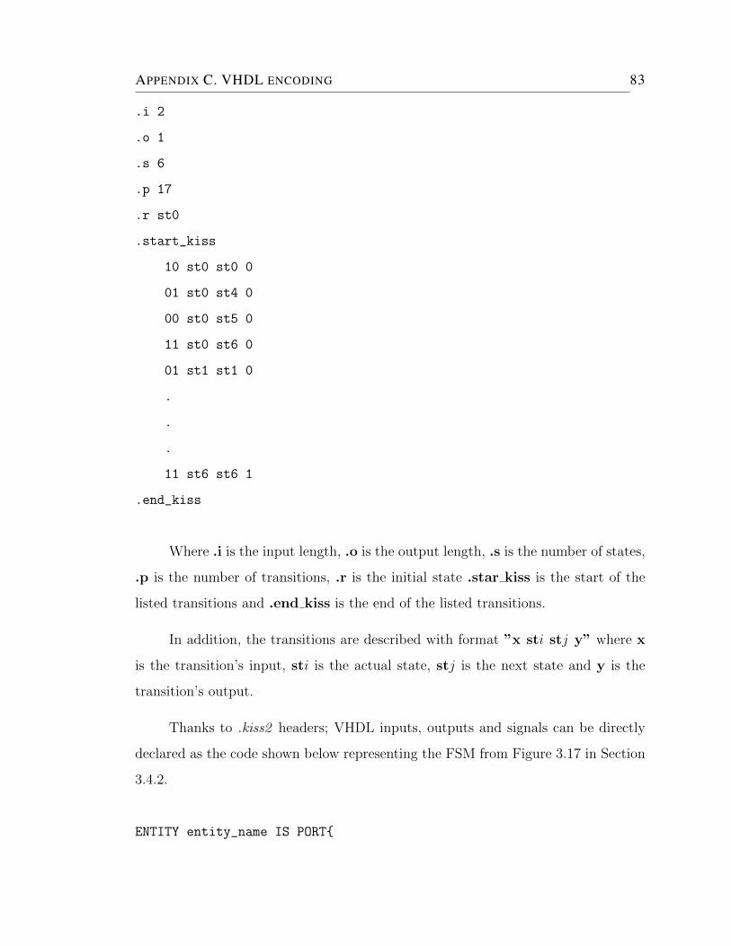
APPENDIX C. VHDL ENCODING 83
.i 2
.o 1
.s 6
.p 17
.r st0
.start_kiss
10 st0 st0 0
01 st0 st4 0
00 st0 st5 0
11 st0 st6 0
01 st1 st1 0
.
.
.
11 st6 st6 1
.end_kiss
Where .i is the input length, .o is the output length, .s is the number of states,
.p is the number of transitions, .r is the initial state .star kiss is the start of the
listed transitions and .end kiss is the end of the listed transitions.
In addition, the transitions are described with format ”x sti stj y” where x
is the transition’s input, sti is the actual state, stj is the next state and y is the
transition’s output.
Thanks to .kiss2 headers; VHDL inputs, outputs and signals can be directly
declared as the code shown below representing the FSM from Figure 3.17 in Section
3.4.2.
ENTITY entity_name IS PORT{
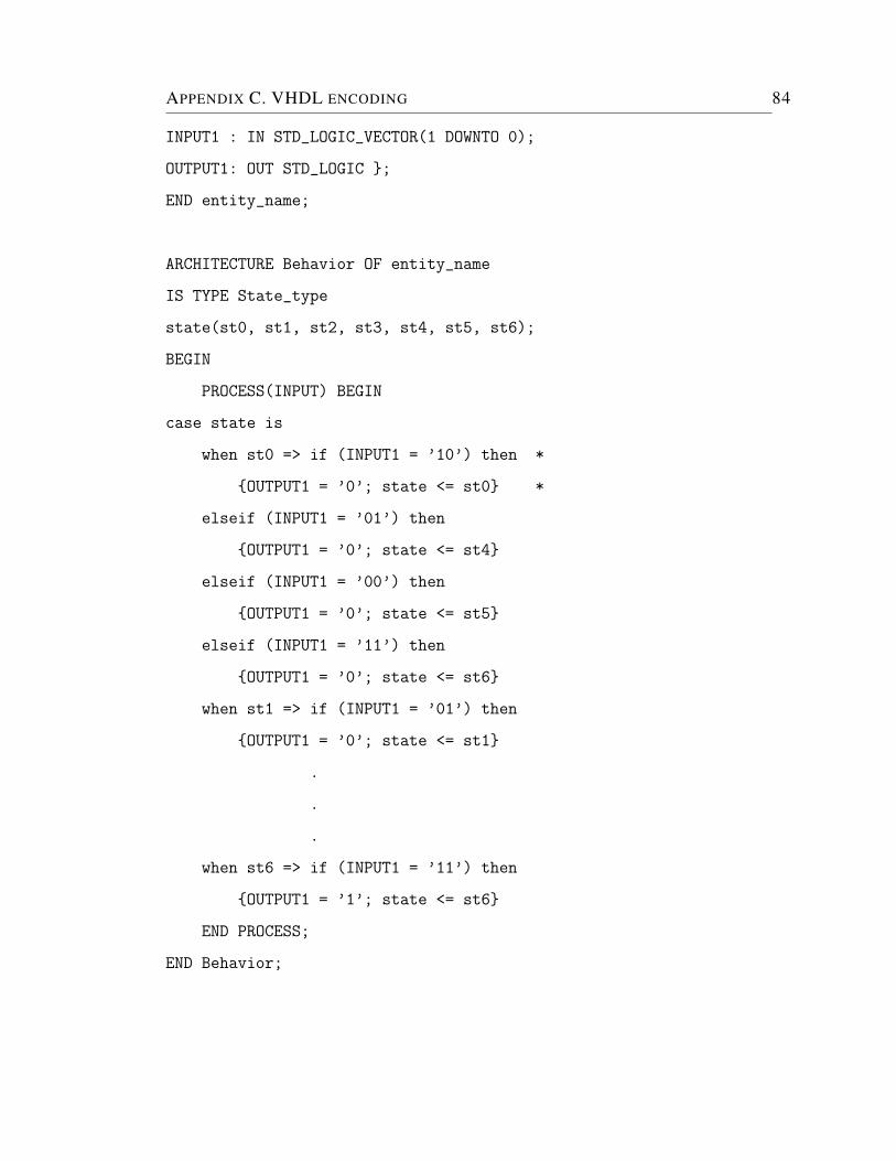
APPENDIX C. VHDL ENCODING 84
INPUT1 : IN STD_LOGIC_VECTOR(1 DOWNTO 0);
OUTPUT1: OUT STD_LOGIC };
END entity_name;
ARCHITECTURE Behavior OF entity_name
IS TYPE State_type
state(st0, st1, st2, st3, st4, st5, st6);
BEGIN
PROCESS(INPUT) BEGIN
case state is
when st0 => if (INPUT1 = ’10’) then *
{OUTPUT1 = ’0’; state <= st0} *
elseif (INPUT1 = ’01’) then
{OUTPUT1 = ’0’; state <= st4}
elseif (INPUT1 = ’00’) then
{OUTPUT1 = ’0’; state <= st5}
elseif (INPUT1 = ’11’) then
{OUTPUT1 = ’0’; state <= st6}
when st1 => if (INPUT1 = ’01’) then
{OUTPUT1 = ’0’; state <= st1}
.
.
.
when st6 => if (INPUT1 = ’11’) then
{OUTPUT1 = ’1’; state <= st6}
END PROCESS;
END Behavior;

APPENDIX C. VHDL ENCODING 85
After declaring ENTITY; the PROCESSES from the ARCHITECTURE
are filled with cases which, at the same time, has whens to represent transitions. For
example, the lines marked with a (*) symbol, indicate that when the actual state is
st0 with an input ’01’, the output will be ’0’ and the next state will return to st0
as shown in Figure C.1.
Figure C.1: Next State example
Thus, it is only necessary to iterate through all states from the FSM to obtain
its transitions and translate them into VHDL.
Bibliography
[1] Leonardo spectrum synthesis, 2012.
http://www.mentor.com/products/fpga/synthesis/leonardo spectrum/. Ac-
cessed: 2013-12-18.
[2] Amr T Abdel-Hamid, Sofiene Tahar, and El Mostapha Aboulhamid. A public-
key watermarking technique for ip designs. In Proceedings of the conference
on Design, Automation and Test in Europe-Volume 1, pages 330–335. IEEE
Computer Society, 2005.
[3] Amr T Abdel-Hamid, Mohamed Zaki, and Sofiene Tahar. A tool converting
finite state machine to vhdl. In Electrical and Computer Engineering, 2004.
Canadian Conference on, volume 4, pages 1907–1910. IEEE, 2004.
[4] Patrick Adenis, Kushal Mukherjee, and Asok Ray. State splitting and state
merging in probabilistic finite state automata. In American Control Conference
(ACC), 2011, pages 5145–5150. IEEE, 2011.
[5] Imtiaz Ahmad and A Shoba Das. A heuristic algorithm for the minimization of
incompletely specified finite state machines. Computers & Electrical Engineer-
ing, 27(2):159–172, 2001.
[6] Shangari.B Arunkumar.P. A new fsm watermarking method to making author-
ship proof for intellectual property of sequential circuit design using stg. Inter-
86
BIBLIOGRAPHY 87
national Journal of Modern Engineering Research, 2(6):4159–4161, November-
December 2012.
[7] Pranav Ashar, Aarti Gupta, and Sharad Malik. Using complete-1-
distinguishability for fsm equivalence checking. In Proceedings of the 1996
IEEE/ACM international conference on Computer-aided design, pages 346–353.
IEEE Computer Society, 1997.
[8] Maria J Avedillo, JM Quintana, and JL Huertas. State merging and state
splitting via state assignment: a new fsm synthesis algorithm. IEE Proceedings-
Computers and Digital Techniques, 141(4):229–237, 1994.
[9] A. Barkalov and L. Titarenko. Logic Synthesis for FSM-Based Control Units.
Lecture Notes in Electrical Engineering. Springer, 2009.
[10] Abhishek Basu, Debapriya Basu Roy, Deep Banerjee, Archan Sengupta,
ANIKET Saha, TIRTHA SANKAR Das, and Subir Kumar Sarkar. Fpga im-
plementation of ip protection through visual information hiding. International
Journal of Engineering Science and Technology, 3(5):4191–4199, 2011.
[11] CBL. The benchmark archives at cbl (up to 1996), December 2007.
http://www.cbl.ncsu.edu/benchmarks/Benchmarks-upto-1996.html.
[12] Edoardo Charbon and Ilhami Torunoglu. Watermarking techniques for elec-
tronic circuit design. In Digital Watermarking, pages 147–169. Springer, 2003.
[13] Santanu Chattopadhyay, Pankaj Yadav, and Ravi Kishore Singh. Multiplexer
targeted finite state machine encoding for area and power minimization. In India
Annual Conference, 2004. Proceedings of the IEEE INDICON 2004. First, pages
12–16. IEEE, 2004.
[14] Hadjicostis Christoforos N. Finite-state machine embeddings for nonconcurrent
error detection and identification. Computer-Aided Design of Integrated Circuits
and Systems, IEEE Transactions on, (2):142–153, 2005.
BIBLIOGRAPHY 88
[15] Aijiao Cui, Chip-Hong Chang, Sofiene Tahar, and Amr T Abdel-Hamid. A
robust fsm watermarking scheme for ip protection of sequential circuit design.
Computer-Aided Design of Integrated Circuits and Systems, IEEE Transactions
on, 30(5):678–690, 2011.
[16] Aijiao Cui, Chip-Hong Chang, and Li Zhang. A hybrid watermarking scheme
for sequential functions. In Circuits and Systems (ISCAS), 2011 IEEE Inter-
national Symposium on, pages 2333–2336. IEEE, 2011.
[17] Agoston E. Eiben and J. E. Smith. Introduction to Evolutionary Computing.
SpringerVerlag, 2003.
[18] O. Garnica, J. Lanchares, and J.M. Sanchez. Finite state machine optimization
using genetic algorithms. In Genetic Algorithms in Engineering Systems: Inno-
vations and Applications, 1997. GALESIA 97. Second International Conference
On (Conf. Publ. No. 446), pages 283–289, Sep 1997.
[19] M. Gen and R. Cheng. Genetic Algorithms and Engineering Optimization. A
Wiley-Interscience publication. Wiley, 2000.
[20] Sezer Goren and F Joel Ferguson. On state reduction of incompletely specified
finite state machines. Computers & Electrical Engineering, 33(1):58–69, 2007.
[21] Antonio Grasselli and Fabrizio Luccio. A method for minimizing the number of
internal states in incompletely specified sequential networks. Electronic Com-
puters, IEEE Transactions on, (3):350–359, 1965.
[22] G.D. Hachtel and F. Somenzi. Logic Synthesis and Verification Algorithms.
Springer, 2006.
[23] David Harris and Sarah Harris. Digital Design and Computer Architecture,
Second Edition. Morgan Kaufmann, 2012.
BIBLIOGRAPHY 89
[24] Rohit Jnagal. Powder: A low power fsm partitioner. n.d., 2008.
http://www.ee.iitb.ac.in/˜microel/download/powder.html. Accessed: 2013-11-
14.
[25] David S Johnson and M Garey. Computers and intractability: A guide to the
theory of np-completeness. Freeman&Co, San Francisco, 1979.
[26] AB. Kahng, J. Lach, W.H. Mangione-Smith, S. Mantik, IL. Markov, M. Potkon-
jak, P. Tucker, Huijuan Wang, and G. Wolfe. Constraint-based watermarking
techniques for design ip protection. Computer-Aided Design of Integrated Cir-
cuits and Systems, IEEE Transactions on, 20(10):1236–1252, Oct 2001.
[27] T Kalker. Considerations on watermarking security. IEEE International Work-
shop on Multimedia Signal Processing, pages 201–206, 2001.
[28] S. Kanjilal, S.T. Chakradhar, and V.D. Agrawal. Test function embedding
algorithms with application to interconnected finite state machines. Computer-
Aided Design of Integrated Circuits and Systems, IEEE Transactions on,
14(9):1115–1127, Sep 1995.
[29] Stefan Katzenbeisser and Fabien A. Petitcolas, editors. Information Hiding
Techniques for Steganography and Digital Watermarking. Artech House, Inc.,
Norwood, MA, USA, 1st edition, 2000.
[30] Jan Kubek. Localisation of the finite state control in the ip cores. In Proceedings
of the 12th Conference STUDENT EEICT 2006 Volume, pages 456–461. Brno
University of Technology, 2006.
[31] J. Lach, W.H. Mangione-Smith, and M. Potkonjak. Fpga fingerprinting tech-
niques for protecting intellectual property. In Custom Integrated Circuits Con-
ference, 1998. Proceedings of the IEEE 1998, pages 299–302, May 1998.
[32] A. Laughton and D.F. Warne. Electrical Engineer’s Reference Book. Elsevier
Science, 2002.
BIBLIOGRAPHY 90
[33] D. Lee and Mihalis Yannakakis. Principles and methods of testing finite state
machines-a survey. Proceedings of the IEEE, 84(8):1090–1123, Aug 1996.
[34] Matthew Lewandowski, Richard Meana, Matthew Morrison, and Srinivas
Katkoori. A novel method for watermarking sequential circuits. In Hardware-
Oriented Security and Trust (HOST), 2012 IEEE International Symposium on,
pages 21–24. IEEE, 2012.
[35] Wei Liang, Xingming Sun, Zhiqiang Ruan, and Jing Long. The design and
fpga implementation of fsm-based intellectual property watermark algorithm at
behavioral level. Information Technology Journal, 10(4), 2011.
[36] Bill Lin, Herve J Touati, and A Richard Newton. Don’t care minimization of
multi-level sequential logic networks. In Computer-Aided Design, 1990. ICCAD-
90. Digest of Technical Papers., 1990 IEEE International Conference on, pages
414–417. IEEE, 1990.
[37] Chien-Nan Liu and Jing-Yang Jou. A fsm extractor for hdl description at rtl
level. In Asia Pacific Conference on Hardware Description Languages, pages
33–38. Citeseer, 1998.
[38] Chien-Nan Jimmy Liu and Jing-Yang Jou. An automatic controller extractor
for hdl descriptions at the rtl. IEEE Design & Test of Computers, 17(3):72–77,
2000.
[39] G. Athisha M. Meenakumari. A Survey on Protection of FPGA Based IP De-
signs. Institute for Research and Development India, 2013.
[40] Alicia Morales-Reyes. Fault Tolerant and Dynamic Evolutionary Optimization
Engines. PhD thesis, College of Science and Engineering, The University of
Edinburgh, 2010.
[41] D. Mukherjee, M. Pedram, and M. Breuer. Merging multiple fsm controllers
for dft/bist hardware. In Computer-Aided Design, 1993. ICCAD-93. Digest of
BIBLIOGRAPHY 91
Technical Papers., 1993 IEEE/ACM International Conference on, pages 720–
725, Nov 1993.
[42] Marvin C Paull and Stephen H Unger. Minimizing the number of states in
incompletely specified sequential switching functions. Electronic Computers,
IRE Transactions on, (3):356–367, 1959.
[43] Jorge M Pena and Arlindo L Oliveira. A new algorithm for exact reduction of
incompletely specified finite state machines. Computer-Aided Design of Inte-
grated Circuits and Systems, IEEE Transactions on, 18(11):1619–1632, 1999.
[44] Andrey Popov and Krasimira Filipova. Genetic algorithms-synthesis of finite
state machines. In Electronics Technology: Meeting the Challenges of Electron-
ics Technology Progress, 2004. 27th International Spring Seminar on, volume 3,
pages 388–392. IEEE, 2004.
[45] Bart Preneel, Hans Dobbertin, and Antoon Bosselaers. The cryptographic hash
function ripemd-160.
[46] Codrin Pruteanu and C Haba. Genfsm: A finite state machine generation tool.
Proc. 9th Int. Conf. Dev. Applicat. Syst, pages 165–168, 2008.
[47] June-Kyung Rho, Gary D Hachtel, Fabio Somenzi, and Reily M Jacoby. Exact
and heuristic algorithms for the minimization of incompletely specified state
machines. Computer-Aided Design of Integrated Circuits and Systems, IEEE
Transactions on, 13(2):167–177, 1994.
[48] JM Sanchez, AO Garnica, and J Lanchares. A genetic algorithm for reducing the
number of states in incompletely specified finite state machines. Microelectronics
journal, 26(5):463–470, 1995.
[49] Shlomo S Sawilowsky. Misconceptions leading to choosing the t test over the
wilcoxon mann-whitney test for shift in location parameter. 2005.
BIBLIOGRAPHY 92
[50] VV Solov’ev. Minimization of mealy finite state machines via internal state
merging. Journal of Communications Technology and Electronics, 56(2):207–
213, 2011.
[51] VV Solov’ev. Complex minimization method for finite state machines imple-
mented on programmable logic devices. Journal of Computer and Systems Sci-
ences International, 53(2):186–194, 2014.
[52] I Torunoglu and E. Charbon. Watermarking-based copyright protection of se-
quential functions. Solid-State Circuits, IEEE Journal of, 35(3):434–440, March
2000.
[53] Frank Wilcoxon. Individual comparisons by ranking methods. Biometrics bul-
letin, pages 80–83, 1945.
[54] Wenchao Xu and Yuesheng Zhu. A digital copyright protection scheme for soft-
ip core based on fsms. In Consumer Electronics, Communications and Networks
(CECNet), 2011 International Conference on, pages 3823–3826. IEEE, 2011.
[55] Xia Yinshui, AEA Almaini, and Wu Xunwei. Power optimization of finite state
machine based on genetic algorithm. J. Electron, 20(3), 2003.
[56] Daniel Ziener, Stefan Aßmus, and Jurgen Teich. Identifying fpga ip-cores based
on lookup table content analysis. In Field Programmable Logic and Applications,
2006. FPL’06. International Conference on, pages 1–6. IEEE, 2006.
[57] Daniel Ziener and Jurgen Teich. New Directions for IP Core Watermarking and
Identification. In Peter M. Athanas, Jurgen Becker, Jurgen Teich, and Ingrid
Verbauwhede, editors, Dynamically Reconfigurable Architectures, number 10281
in Dagstuhl Seminar Proceedings, Dagstuhl, Germany, 2010. Schloss Dagstuhl
- Leibniz-Zentrum fuer Informatik, Germany.