finland post-facto comparison - international actuarial … · · 2015-11-25after having first...

WORKSHOP

A S I MULATION P R O C E D U R E FOR C O M P A R I N G D I F F E R E N T CLAIMS RESERVING METH O D S

BY TEIVO PENTIK,~INEN AND J U K K A R A N T A L A

Finland

A B S T R A C T

The estimation of outstanding claims is one of the important aspects in the management of the insurance business. Various methods have been widely dealt with in the actuarial literature. Exploration of the inaccuracies involved is traditionally based on a post-facto comparison of the estimates against the actual outcomes of the settled claims. However, until recent years it has not been usual to consider the inaccuracies inherent in claims reserving in the context of more comprehensive (risk theoretical) models, the purpose of which is to analyse the insurer as a whole. Important parts of the technique which will be outlined in this paper can be incorporated into over-all risk theory models to introduce the uncertainty involved with technical reserves as one of the components in solvency and other analyses (PENTIKAINEN et al. (1989)).

The idea in this paper is to describe a procedure by which one can explore how various reserving methods react to fictitious variations, fluctuations, trends, etc. which might influence the claims process, and, what is most important, how they reflect on the variables indicating the financial position of the insurer. For this purpose, a claims process is first postulated and claims are simulated and ordered to correspond to an actual handling of the observed claims of a fictitious insurer. Next, the simulation program will 'mime ' an actuary who is calculating the claims reserve on the basis of these 'observed ' claims data. Finally, the simulation is further continued thus generating the settlement of the reserved claims. The difference between reserved amounts and settled amounts gives the reserving (run-off) error in this particular simulated case. By repeating the simulation numerous times (Monte Carlo method) the distribution of the error can be estimated as well as its effect on the total outcome of the insurer.

By varying the assumptions which control the claims process the sensitivity of the reserving method visa-5,-vis the assumed phenomena can be tested. By applying the procedure to several reserving methods in parallel a conception of their properties can be gained, in particular, how robust they are against various variations and irregularities in the claims process.

It is useful to recognize and classify error sources which give rise to the reserving inaccuracies (cf. PENTIK.~INEN et al. (1989) item 2.4b): 1) The model (often simply called reserving rule or formula or method) can be

only a more or less idealized description of the real world and of the actual

ASTIN BULLETIN, Vol. 22, No. 2, 1992

192 TEIVO PENTIK,~INEN AND JUKKA RANTALA

claims settlements; the deviations give rise to what can be termed model errors.

2) The parameters used in calculations are subject to parameter errors owing to the fact that they are to be estimated from various data statistics or found from other more or less uncertain sources.

3) The actual claims and claims settlements are subject to stochastic fluctuations causing deviations from the estimates, stochastic errors, even in those (theoretical) cases where the model and its parameters would be precisely correct.

The above procedure enables us to examine the effects of all these three errors, in fact, it is very general, not being restricted to any specific reserving model or assumptions on the claims process. It is intended for studies of the properties of the reserving methods on a general level. However, it is not meant for post-facto analyses, i.e. in the investigation and estimation of the inaccuracies in reserves in particular concrete cases, for those purposes well-known actuarial and statistical approaches are needed.

It is still worth noting that the approach can find application to other estimations as well. We have, for instance, also treated premiums in an analogous way, although limited to simple examples in this paper.

After having first described our method in general terms a number of numerical examples will be given to illustrate some of its relevant features. They are based on some well-known elementary reserving rules and simple assumptions on the claims process. Also some conclusions on the properties of the reserving rules are derived therefrom. They should be understood merely as examples of the use of our model, not as any real analyses of the reserving methods. Even though our method is aimed at making such conclusions and comparisons between methods, their pertinent performance would require quite extensive studies. Such have been fully beyond the possibilities in this context.

KEYWORDS

Claims reserving; run-off errors; chain ladder; model errors; parameter errors; simulation.

1. BASIC CONCEPTS

1.1. References to related works

A summary of the claim reserving techniques was compiled by VAN EEGHEN (1981). Furthermore, the monograph by TAYLOR (1986) is referred to as is the recent Claims Reserving Manual (1989) of the UK Institute of Actuaries. Enhanced methods for analyses, among others regarding the above listed sources of errors, have been recently proposed, for example, by ASHE (1986), NORBERG (1986), SUNDT (1990) and WRIGHT (1990).

PROCEDURE FOR COMPARING DIFFERENT CLAIMS RESERVING METHODS 193

The run-off errors, as a source of uncertainty in solvency considerations, were dealt with by the Britisch Solvency Working Party in a series of reports: DAYKIN et al. (1984), . . . , DAYKIN and HEY (1990). STANARD (1986), REN- SHAW (1989), VERRALL (1989), (1990) have analysed the properties of the chain ladder method.

The stochastic claim run-off error was analysed by PENTIK~INEN and RANTALA (1986) to which this paper is a continuation. The results were incorporated as a submodel into the application-orientated risk theoretical over-all model in PENTIK,~INEN et al. (1989).

We are going to use, as far as possible, the notations and concepts used in the above-referred papers. However, the terminology adopted in the Manual of IA (1989) is also taken into account. For the convenience of the reader the main features are recapitulated.

1.2. Claims cohorts

In order to clarify the terminology and the notation it is useful to note that the claim process includes the following elements:

l) the event (accident) which cases a claim in year t.

2) The claim is reported to the insurer in year t or later.

3) The claim is settled in year t+s(s _> O) or possibly in several parts in years I - I - S i , l ' + s 2 , . . .

4) If the claim is reported by the end of the accounting year but not yet fully settled, it is called open and a provision is made to meet the outstanding liability either as a case estimate or by using some statistical technique.

5) The claims which are incurred but not yet reported by the end of the accounting year are " IBNR-cla ims"

Following the terminology of Manual of IA (1989) (A 5.1) outstanding claims is an umbrella concept for open and IBNR claims.

It is appropriate to group the claims originating in the same accident year, t, as a "cohor t " . The year t is also called the year of origin. Figure 1.1 illustrates the structure of a cohort and its development.

The accumulated amount of settled claims from development years t, t + 1, t + 2 . . . . . t+s supplemented by the provision of the open claims at the end of year t+s is called, still following the terminology of Manual of IA (1989, p. A5.2, the incurred loss and is denoted by

(I.1) X( t ;O , s )=c la ims originating from year t and paid in years t, t+ 1, . . . , t+s on settled or partially settled claims plus reserve held for the open claims at the end of year t+s.

A notation for the increments of X is also needed:

(1.2) X(t; sl, s2) = X(t; O, s z ) - X ( t ; O, s t - 1)

194

Accumulated clolms X

TEIVO P E N T I K , ~ I N E N A N D J U K K A R A N T A L A

t t + $ t + $n.~:~¢

FIGURE 1.1. The d e v e l o p m e n t o f a c la ims c o h o r t .

and especially

(1.3) X(t; s, s) = X(t; O, s ) - X ( t ; O, s - 1)

which is the increment in the development year t+s (by convention, X(t; O, - 1) = 0).

It is assumed that after some period Smax all claims of the origin year t are settled. The parameter Smax characterizes a feature of the portfolio which is called the length of the run-off tail. Hence, the development time variable s can have values O, 1, . . . , Smax, and,

(1.4) X(t; O, Smax) is the final total amount of claims of the cohort t.

It is also called the loss related to the cohort.

1.3. The reserve for IBNR claims of the cohort t at the end of year t+s is defined as :

(1.5) C(t, s) = Estimate for {X(t; s + I, Smax) } .

Various methods, 'reserving rules', can be applied in this estimation. The purpose of this paper is to find methods and measures .[or the evaluation of the uncertainty involved with the rules.

Concept (1.5) is in conformity with the " L o n d o n marke t" definition presented in the Manual of IA (1989), p. A5.1 where the IBNR-reserve is defined to be equal to the estimated ultimate loss on all outstanding claims less the reserve at the accounting date for open claims. Hence, the uncertainty in the reserve of open claims is included within that of the IBNR-reserve, as thus defined. As stated in the next paragraph, this type of definition seems to be


convenient in this context, because it allows the collective handling of all kinds of uncertainties in claims process. Note that this definition is different from the common accounting practice according to which the provisions for both the open claims and IBNR's are included in the claims reserve.

No safety margins are assumed to be included in the reserve.

1.4. Claims process

The model to be employed is based on the fact that the increment X(t; s, s) is made up of the sum of changes in the status of individual claims. It is helpful to classify "change-causing events" as follows:

I) A claim is reported and added to the paid and/or open claims.

2) An open claim, k, is fully or partly settled in year t+s, the amount being Sk(t, s). For it (possibly) a reserve (case estimate) Ck(t, s - l) was made at the end of the preceding year and now can be released. Then

(1.6) Xk(t,s) = Sk(t ,s)--Ck(t ,s--1) (s> I)

contributes to the change of the cohort 's aggregate loss X(t; s, s). If Ck were exactly correct, then Xk would, of course, be zero, but in practice it will often be non-zero (-4-).

3) The provision Ck for an open claim is changed (possibly without any payment action), for instance, if new information has been obtained.

Both 1) the number of events and 2) the amount of the changes involved in, Xk(t,s) above, are random variables. Our techniques, both simulation and others (PENTIK~INEN and RANTALA (1986)), are based on utilizing probability distributions for both of them. Note that the approach is analogous to that of risk theory. Thanks to FILIP LUNDBERG, HARALD CRAMER and others the collective approach replaced the earlier "individual risk theory" . The number of claims and their size are handled as a "r isk process" without reference to the files of the individual policies which actually are behind the claims. The philosophy proved enormously fruitful notwithstanding that the theory can also be built on the individual bases.

As in general collective risk theory and even still more in the context of claims cohort processes it is crucially important to account for the correlations between the development cells of the cohorts as well as the correlations between consecutive cohorts.

Furthermore, note that the claim size variable X k may also be negative. This can be the case particularly in classes 2) and 3) above. This feature should be kept in mind when the risk theory formulae and distributions are built up (cf. BEARD et al. (1984), Section 1.3, p. 7).

For illustration of the approach numerical examples will be exhibited in Section 4, therefore, some basic features of the claims process need to be specified. This is done in the Appendix. We recall that irrespective of which approach is applied in defining the concept of claim development the technique we are going to present can, with obvious modifications, also be applied to

196 TEIVO PENTIKAINEN AND JUKKA RANTALA

claims processes defined otherwise than the collective one. For example, the procedure allows for the use of the bootstrapping technique for claims simulation (as was remarked by one of the referees of this paper).

1.5. T h e a g g r e g a t e loss process related to the whole business of the insurer consists of the sum of the cohort variables X.

Following the practice adopted by NORBERG (1986) a diagram of the Lexis type is constructed in Figure 1.2. The data array representing a cohort develops as an ascending diagonal. The information which the actuary, or in our simulation the computer, has available for the reserve calculation is in the "run-off trapezium" (in the diagram the vertical pillar at the accounting year t and the area left therefrom). The claims to be estimated for the reserve for outstandings are inherent in all of the still open cohorts and are located in the "triangle of outstandings" right from the column at t:

(1.7) C(t) = ~ C(t-s , s). s ~ t

NOTE. The problem in premium rating is basically the same as in the claims reserving. An estimate for the amount of claims of future cohorts is required. The difference in the claims reserving is that only present and past cohorts are considered and that a number of the earliest notified claims are already known and the estimation is focused to the remaining ones only. It is a bit surprising that the methods developed for premium rating are only little utilized in claims reserving.

E

QJ

E 0

>

Tlag Sma x . . . . . . . . . . . . . . . , ............................................

trapeziun _

x(t-~:o,~/ ~ ~ Accident and

cur renLt ime

L - T - s t - s t t + s ~ ' ~ la E m a x m a x

FIGURE 1.2. Claims process as a sum of cohorts. The current accounting year is denoted by t and the cohort originating in the accident year t - s is represented by an ascending diagonal.


2. RUN-OFF ERROR

2.1. Run-off error, break-up consideration

The run-off error is the remainder ( ± ) which is left of the reserve C(t) when all the outstanding claims are ultimately settled:

s i n , , - - I

(2.1) R ( t ) = f ( t ) - 2 X(t-s;s+l,smax). s = 0

In practice, of course, R can be determined only when the settlement of (practically) all of the outstandings is completed. Our approach is to compute it by continuing the simulation until all of the terms of the sum in (2.1) are obtained.

2.2. Going-concern consideration

Further, the effect of the run-off error on the aggregate loss X(t) is examined. This variable is the conventional entry for the total amount of the claims in the profit and loss accounts of the standard annual reports. In the terms of the definitions and notations introduced in item 1.3 it is

S m l x - - I

(2.2) X ( t ) = 2 X(t-s;s,s)+C(t)-C(t-1). s=0

As was noted in item 1.3. in our considerations the provision for open claims is included in the X terms, not in C, notwithstanding that this does not accord with the common accounting practice.

2.3. Properties of a good reserving method

For the appreciation of the efficiency of the reserving methods a great variety of optimality criteria are proposed in actuarial literature. From the point of view of the company's management the following features might be the most important :

(1) Probability of insufficiency of the reserve should be small (e), more exactly

(2.3) Prob {R + L < 0} < e

where L is a safety loading. (In practice it can either be included in the claims reserve C(t) in addition to the unbiased estimate (I.5) as an extra margin or e.g. as an equalisation provision or it can be available otherwise as a part of the insurer's solvency margin).

(2) The safety loading L should be as small as possible.

(3) The variation of the aggregate claims in the profit and loss account should be as small as possible (particularly in the going-concern approach).


In the next item some potential measures will be proposed for the comparison of different reserving methods having regard for the above criteria (1)-(3).

2.4. Measures of uncertainty

The run-off error R and its impact on X depend self-evidently on the reserving method. This dependence varies with the different claims processes. We shall use as primary measures in describing these effects both the direct values of R and X and their ratios and the standard deviations aR and ax of these variables together with the ratios

(2.4) aR/C, an/P, a x / e and ax/ao

where P is the premium income corresponding to the relevant X (more in item 3.3). Furthermore, a0 is the standard deviation of Xo(t) which is the incurred aggregate loss from which the run-off error is removed. This is obtained from the simulated data, in terms of our notations, Xo(t ) = X(t; 0, Smax) (= the total loss related to the cohort t). Hence, the difference a x - a o is to be credited to run-off error.

Let us also recall that indicators based on the ditribution of extreme deviations or confidence intervals, are good candidates as measures (cf. PENTIK.~INEN and RANTALA (1986)), but at this stage of work we mainly used the standard deviations. They need less simulations, but involve the drawback that the effect of skewness of the distributions is partly lost.

Note that when in the following illustrate the comparison of two or more reserving rules, the very same claim pattern X(t; s, s) is used for all of them. Therefore, it can be expected that the differences revealed in results can be credited to the differing structures of the rules.

3. RESERVING METHODS USED IN THE CASE STUDIES

3.1. Chain Ladder method

This well-known method is chosen as the first of our test examples. It operates auxiliary development coefficients

(3.1) d(s) = Ai (s)/Ao(s).

Where the A's represent the sums of all X ( t - u ; v, v) located in the areas marked by the same symbols in Figure 3.1a.

The claim sums to be estimated for the remaining parts of the cohorts are now obtained by assuming that the cohorts grow in the same proportion as the parallelograms A, i.e.

X ( t - s ; O, s+ 1) = X ( t - s ; O, s) .d(s)

X ( t - s ; O, s+ 2) = X ( t - s ; O, s+ l ) - d ( s + 1) = X ( t - s ; O, s ) .d ( s ) .d ( s+ 1)


k x Ttag

/ " . / S rn~x

. / / " ../"

Si X L ,Ao,/

t -s t - s - i t m a x

~x

t - s

f i ,

t+u

a) A l(s ) is the parallelogram shaded in the b) Development of a cohort. diagram, and Ao(s ) is obtained by removing the top-most row from A~.

FIGURE 3.1. Derivation of the Chain Ladder rule.

etc. Hence, the claims reserve for the cohort t - s is

(3.2)

where

C ( t - s , s) = x ( t - s ; O, s).c~_. (s),

Stun I -- ]

(3.3) c ~ - I ( s ) = H d(s+u)-I u = 0

and the total claims reserve at the end of the accounting year t is

Sma t -- [

(3.4) C(t) = E C(t-s,s). s = 0

Note that cc-i (s) should be recalculated in each accounting year t (hence, a notation cc_ l(t, s) would, perhaps, be more advisable).

The Chain Ladder rule is at its best in the cases where the so-called structural (also called mixing) variation is large. This is a well-known feature and is again confirmed by the numerical example to be set out later as well as also in PENTIK~,INEN and RANTALA (1986, Appendix 1).

3.2. A variant

The chain ladder method can be amended by broadening the " ru n -o f f triangle" to a trapezium from which the parallelograms A are cut, if this is available. The dotted line associated with a "broadening parameter" Ttag (see Fig. 1.2 and 3.1) refers to this variant. Its effect will be tested in Section 4.4 below.


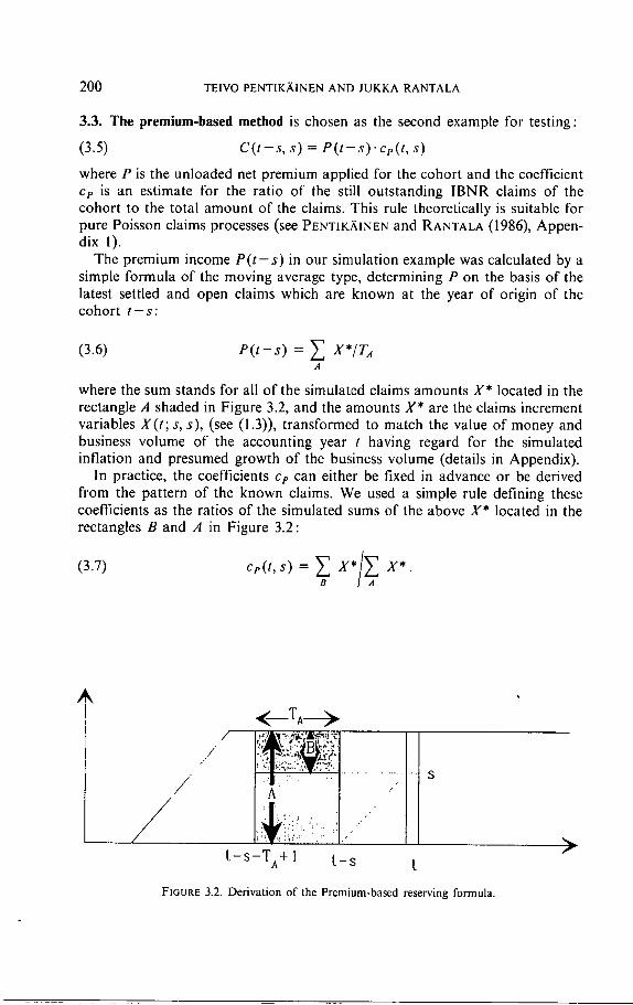
3.3. The premium-based method is chosen as the second example for testing:

(3.5) C(t-s , s) = P(t -s) 'ce( t , s)

where P is the unloaded net premium applied for the cohort and the coefficient Cp is an estimate for the ratio of the still outstanding IBNR claims of the cohort to the total amount of the claims. This rule theoretically is suitable for pure Poisson claims processes (see PENTIK,~INEN and RANTALA (1986), Appen- dix 1).

The premium income P( t - s ) in our simulation example was calculated by a simple formula of the moving average type, determining P on the basis of the latest settled and open claims which are known at the year of origin of the cohort t - s :

(3.6) P( t - s ) = ~ X*/TA A

where the sum stands for all of the simulated claims amounts X* located in the rectangle A shaded in Figure 3.2, and the amounts X* are the claims increment variables X(t; s, s), (see (1.3)), transformed to match the value of money and business volume of the accounting year t having regard for the simulated inflation and presumed growth of the business volume (details in Appendix).

In practice, the coefficients Ce can either be fixed in advance or be derived from the pattern of the known claims. We used a simple rule defining these coefficients as the ratios of the simulated sums of the above X* located in the rectangles B and A in Figure 3.2:

(3.7) C p ( t , s ) = ~ X * / ~ X*.

. /

/

/

~--TA--->

t -s-TA+ I t - s

FIGURE 3.2. Derivation of the Premium-based reserving formula.

f


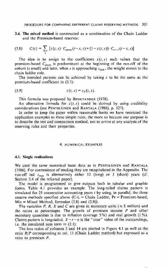
3.4. The mixed method is constructed as a combination of the Chain Ladder and the Premium-based reserves:

(3 .8) C(t) = E [z(l's)'CP rem(l-S's)+(]-g(l'S))'Cc-I(l-S'S)] S

The idea is to assign to the coefficients z( t ,s) such values that the premium-based Cprem is predominant at the beginning of the run-off of the cohort (s small) and later, when s is approaching Smax, the weight moves to the chain ladder rule.

The intended purpose can be achieved by taking z to be the same as the premium-based coefficient in (3.7):

(3.9) z(t, s) = Ce(t, s).

This formula was proposed by BENKTANDER (1976). An alternative formula for z( t ,s) could be derived by using credibility

considerations (see PENTIKAINEN and RANTALA (1986), p. 127). In order to keep the paper within reasonable limits we have restricted the

application examples to these simple rules, the more so because our purpose is to describe the test and comparison method, not to arrive at any analysis of the reserving rules and their properties.

4. NUMERICAL EXAMPLES

4.1. Single realisations

We used the same numerical basic data as in PENTIK,~INEN and RANTALA (1986). For convenience of reading they are recapitulated in the Appendix. The run-off tail Smax is alternatively either 12 (long) or 3 (short) years (cf. Section 3.4 of the referred paper).

The model is programmed to give outputs both in tabular and graphic forms. Table 4.1 provides an example. The long-tailed claims pattern is simulated for 25 consecutive accounting years t by using, ill parallel, the three reserve methods specified above (C-L = Chain Ladder, Pr = Premium-based, Mix = Mixed Method, formulae (3.8) and (3.9)).

The variables P, R, X and C are given in monetary units ( ~ $ million) and the ratios as percentages. The growth of premium income P and other monetary quantities is due to inflation (average 5%) and real growth (1%). Claims pattern is long-tailed. X - r - o is the " t r u e " value of the outstandings, i.e. the simulated sum term in (2.1).

The loss ratios of columns 3 and 14 are plotted in Figure 4.1 as well as the ratio R/P corresponding to col. 11 (Chain Ladder method) but expressed as a ratio to premium P.

2 0 2 TEIVO PENTIK,~INEN AND JUKKA RANTALA

TABLE 4.1

SIMULATED RUN-OFF ERRORS R AND THE AGGREGATE LOSSES X

I 2 3 4 5 6 7 8 9 10 11 12 13 14 15 16

t P Xo/P% X-r-o C(t) R(t) R(t)/C(t)% X(t)/P% C-L Pr Mix C-L Pr Mix C-L Pr Mix C-L Pr Mix

0 65.7 83.8 175.6 184.4 189.8 188.4 1 68.8 98.6 187.3 196.1 197.3 194.2 2 71.0 89.6 195.0 186.4 205.2 193.2 3 73.4 99.2 206.7 183.3 213.1 198.0 4 75.8 107.6 225.3 209.8 221.0 214.5 5 80.4 120.4 248.9 237.6 230.8 227.7 6 85.0 104.5 257.5 260.0 241.5 243.3 7 90.4 117.9 284.0 273.8 254.7 258.8 8 96.6 100.1 288.2 291.6 270.1 279.8 9 104.6 117.1 317.4 328.6 288.9 300.0

10 114.5 114.1 350.0 360.4 311.8 329.0 11 121.7 95.9 361.1 364.1 335.3 349.5 12 130.2 101.9 388.5 365.8 360.3 370.9 13 143.2 101.3 415.9 365.9 390.4 383.4 14 157.2 98.8 435.7 431.4 423.8 432.3 15 169.2 98.2 467.9 459.1 459.4 464.3 16 183.7 93.4 497.7 429.1 499.3 485.5 17 198.0 95.9 532.7 502.2 541.0 531.7 18 212.2 98.3 571.4 572.1 585.0 586.8 19 220 .9 104.7 634.6 631.7 626.7 633.5 20 233.9 88.0 632.0 742.8 666.6 699.8 21 246.9 95.8 681.3 693.3 708.3 711.1 22 256.7 89.3 695.8 713.1 745.9 742.9 23 275 .2 100.6 744.3 727.9 788.0 754.7 24 286.0 88.4 762.8 764.6 828.8 793.8 25 295.3 92.9 786.3 817.0 865.0 822.3

8.8 14.2 12.8 4.8 7.5 6.8 73.9 94.1 77.0 8.8 10.0 6.9 4.5 5.1 3,6 98.6 92.5 90.0

-8.6 10.2 - I . 8 -4.6 5.0 - .9 65.1 89.9 77.4 -23.4 6.4 -8.6 -12.8 3.0 -4.4 79.1 94.0 89.8 -15.4 -4.3 -10.8 -7.3 -1.9 -5.0 118.1 93.5 104.8 -11.2 -18.1 -21.2 -4.7 -7.8 -9.3 125.6 103.2 107.4

2.6 -16.0 -14.2 1.0 -6.6 -5.8 120.8 107.0 112.7 -10.1 -29.2 -25.2 -3.7 -11.5 -9.7 103.9 103.3 105.8

3.3 -18.1 -8.4 1.1 -6.7 -3.0 114.1 111.6 117.4 11.2 -28.6 -17.5 3.4 -9.9 -5.8 124.5 107.1 108.4 10.3 -38.2 -21.0 2.9 -12.3 -6.4 113.4 105.7 111.0 3.1 -25.8 -11.6 .8 -7.7 -3.3 89.9 106.1 103.6

-22.7 -28.3 -17.6 -6.2 -7.8 -4.7 82.1 100.0 97.3 -50.1 -25.6 -32.5 -13.7 -6.5 -8.5 82.2 103.2 90.9

-4.3 -11.9 -3.4 - I . 0 -2.8 - .8 127.9 107.5 117.3 -8.9 -8.6 -3.6 - I . 9 - I . 9 - .8 95.5 100.2 98.1

-68.6 1.6 -12.2 -16.0 .3 -2.5 60.9 98.9 88.7 -30.4 8.4 - .9 -6.1 1.6 - .2 115.1 99.3 101.5

.7 13.6 15.4 .1 2.3 2.6 113.0 100.8 106.0 -2.9 -8.0 -1.2 - .5 -1.3 - .2 103.1 95.0 97.3 110.8 34.7 67.8 14.9 5.2 9.7 136.7 106.3 117.5 12.0 27.0 29.8 1.7 3.8 4.2 55.8 92.7 80.4 17.3 50.1 47.1 2.4 6.7 6.3 91.3 98.3 96.0

-16.4 43.7 10.4 -2.3 5.5 1.4 88.3 98.3 87.3 1.8 66.0 31.0 .2 8.0 3.9 94.8 96.2 95.6

30.7 78.7 36.0 3.8 9.1 4.4 102.7 97.2 94.6

1 . 5

. 5

- . 5 la

1 X / P

X o / P

• - - i I . . . . I . . . . I i ~ ~ . . I , , , , f

5 10 t5 20 25

FIGURE 4.1. The ratios Xo/P ( - -0 - - ) , X/P ( - - - - ) and R/P. Chain Ladder rule.


100

90

BB

70

GB

50

4~ 5 I~ 15 2~ 25

FIGURE 4.2. The premium income P, dellated into the monetary value of the initial time point, as a (delayed) moving average of the loss X 0.

The ra t io RIP and the dev ia t ion o f X/P f rom X o/P are shaded in o rde r to show the s t rong cor re la t ion between them. When R is increasing, it worsens (increases) the loss ra t io and vice versa. No te that X/P f luctuates more than

' o r i g ina l ' Xo/P. Figure 4.2 depic ts the p r emium income P and the aggrega te " n o n - r u n - o f f

a f f ec t ed" loss X0 from which P is der ived accord ing to (3.6) as a mov ing average with the range 10 years and with a necessary t ime lag. F o r clari ty, the effect o f inf lat ion and growth is s t r ipped away from the t ime series by ope ra t ing the var iables in the initial value o f money and vo lume (at t = 0).

Al l the loss ra t ios X/P of Tab le 4.1 and the ra t ios RIP are p lo t ted in F igure 4.3.

1 .5 L o s s rotlos X/P

~m ~ ~ ~"~. K, , ~.~ l'~t

', i , , i ~' i/

.5

Run-oFF errors R/P " /--\

" ~ ~ w " J " l '~ ~ p > ' p ' i D " ~ . / , ~ ' " ' ~ ' , . h ' ( . . . / ~m. , , " ~ " " ~' ~-~" ~ ~ ~ ~ "" " -

'~., ~.~.... ; ~ P ~ - ~ , ~ / \ l Y ~" "¢ ~'~" "V' 'V'

. . . . I . . . . I , i i i I , i i i I . . . . I

-'50 5 10 15 20 2

FIGURE 4.3. Loss ratios X/P and R/P calculated by using Chain Ladder (marked by c), Premium-based (p) and Mixed (m) methods, respectively. The thick line represents Xo/P.

204 TEIVO PENTII,~INEN AND JUKKA RANTALA

A smoother flow of X/P can be achieved at the expense of larger reserve errors R/P.

Simulations confirm the well-known fact (STANARD (1986) and ZEHNWIRT'S article in the Manual of the IA (1989), Vol. II) that the Chain Ladder method has a tendency to show a greater volatility than the other rules compared.

4.2. Monto Carlo simulations

In order to get broader insights into the behaviour of the target variables the simulations exemplified in Figures 4.1 and 4.3 were repeated 50 times for each of the three rules. " A stochastic bundle" is generated in this way in Figure 4.4.

The breadth of the bundle of the simulated realisations gives an idea of the volatility involved with the reserving methods.

A useful observation, seen in Figure 4.4, is that the bundles are stabilized at about a state of equilibrium, i.e. the breadth of the bundles is approximately constant. This feature appeared to be common in those cases we experimented with apart from some extreme situations (premiums defined deterministically and kept unchanged for a long period), where the bundle could have some tendency to diverge. If a reasonably satisfactory attainment of the equilibrium state can be achieved, then it is possible to record the values of the relevant variables, X/P, etc. at each time point t of the run, and to compute the required standard deviations as "s teady-s ta te" characteristics from the set of all of them. This procedure greatly reduces the number of simulations needed compared with approaches which might require a new simulation for each variable value. Table 4.2 is obtained from Figure 4.4 in this way.

TABLE 4.2

STANDARD DEVIATIONS OF THE SIMULATED RATIOS

Chain Ladder Premium-based Mixed

tr x / P 0.126 0.061 0.102 trx/a o 1.749 0.851 1.414 o'R/P 0.079 0.062 0.066

Similar data will be given for a long-tail pattern in the next item. Therein the obviously characteristic features of the methods are more clearly seen.

4.3. Error distributions

The X/P and R/P values simulated, as shown in Figure 4.4, can be recorded and plotted, as in exhibited in Figure 4.5a and in Figure 4.5b which set out the critical tails of distributions.

Confidence limits can be directly read from the picture. For instance, the limit which the Chain Ladder ratio X/P exceeds by 1% probability, is 1.57.


1.5

1

.5

R,L.MI~¢F Ih."r~" RIP

0

0 5 IO 15 2 0 2 5

C h a i n L a d d e r

'-s t LO l l rltlo X/P

.5

- . 5 0 5 10 15 20 25

P r e m i u m - b a s e d

1.5

I

• s Mixed Run-o t r l r w - ro t R /P

- . 5 B 5 10 15 2B 25

FIGURE 4.4. Monto Carlo smlulation of loss ratios X/P and run-off errors R/P for the three reserve rules. Short tail (Sm~ = 3). Premium rule stochastic moving average (3.3 above). Sample size 50.


1 0 a

11~ -1

I 1~ -2

1~-3 - 1 - . 5 0 . 5 1 ] . 5 2

FIGURE 4.5a. The cumulative distributions F(x) and F(r) for the ratios x = X/P and r = R/P, respectively, are obtained from the simulated patterns of these ratios. For clarity, F is plotted for the left-hand tail of the distributions and 1 - F for the right-hand tails in a semi-logarithmic scale. The number of sample points is 15600 for each curve. Long tail Sma x = 12. Premium method stochastic.

F(r) / . - I -F(x)

I : " / \ ' \ . I

Rpr--'-~-'-/k/l/7/ -- xpr - x 0 " Xmix--- Xc't , ,-, R,,,,__.d.,.C/ \ \.] \,,

/~/"Y \ ~. ' : ' 1 1 \

t 1 / •/~i'i/ ' - . 9 - . 8 - - . 7 - - .G - . 5 - . 4 - - . 3 I 1.1 I . Z 1 .3 1 .4 1 . 5 1 . 6 1 . 7 l . f l

FIGURE 4.5b. The tails of the distributions of Figure 4.5a.

Similarly, the limit, which the Premium-based R/P falls below by 1% probability, is - . 58 .

Note that the distributions exhibited in Figure 4.5 are based on the development tail of 12 years which is rather long and, on the other hand, on the portfolio which is relatively small, the average number of claims being 10000.

For a comparison of the exemplified reserving methods, the standard deviations derived from the same simulation as Figure 4.5 are shown in Table 4.3.

PROCEDURE FOR COMPARING DIFFERENT CLAIMS RESERVING METHODS

TABLE 4.3 TTHE BASIC CHARACTERISTICS RELATED TO THE DISTRIBUTIONS OF FIGURE 4.5

207

St.dev Rel.st.d. Variable Mean ¢7 O'/O" 0

Xo; - -/P 1.003 .087 1.000 X; c-liP 1.001 .240 2.759 X; pre/P .980 .065 .745 X; mix/P .993 .125 1.431 R; c-liP -.002 .259 2.979 R; pre/P .039 .267 3.066 R; mix/P .004 .221 2.534

The mean values are shown in the table to verify that they are, as they theoretically should be, close to unity for X/P's and zero for R/P's (in order to check that the simulation variability and programming are under control).

In extreme cases the skewness of the distribution may be considerable and might suggest that it should be seriously regarded in order to avoid the caveat of understating the run-off risk. Some tests (not set out in this paper) also indicated rather great volatility in the development of the tails. We had to leave further studies on this problem for later work.

A feature of interest is the smoothing effect of the premium-based rule. The Premium-based rule, in fact, reduces the range of fluctuation of the loss ratio X/P compared with the case Xo/P from which the run-off error is eliminated. This happens, of course, at the expense of larger run-off errors R/P, as seen in Figures 4.3-4.5 and Table 4.3 when comparing the premium based rule to the mixed one. The adverse tops of the fluctuation of X are spread over a lengthy period.

As expected, the performance of the chain ladder in these examples proved to be rather poor in regard to both the loss ratio and run-off error.

4.4. Stability profiles

The tools developed in the preceding sections are now readily available for the comparison of different reserving methods. We exemplify the idea by applying it to the three methods which were specified in Section 3. For the purpose, the standard deviations ax, aR and a0 are calculated in parallel. Figure 4.6 exhibits an example. The relevant indicators are plotted as columns in order to provide a clear view of their magnitudes. Various patterns of the claim process are simulated for all the three reserving methods. They are constructed from the standard data by allowing options and inserted special variations, as explained in the captions of the figures. The standards are the same as we had in PENTIKAINEN and RANTALA (1986) and a summary is given in the Appendix below.

The left-hand displays of Figure 4.6 represent the relevant standard deviations as ratios to the premium income P. In order to show more clearly the role


ox/P

1 2 3 4 5 1 2 3 4 5 , 2 3 4 5 12345 NO-- to t h a i n - k p r l b a S H I x

oR/P

_ _ °x/°o

I ~ 3 1 5 1 2 3 ' 1 1 5 NO--CO

@ 1 2 3 4 5

Cha I n - L Pr -bmm 12345

Mix

4

.3

2

FIGURE 4.6. Stability profiles. The numbered claims process options processed in parallel are as follows:

1) Short tail, stochastic premium rule (the same as Fig. 4.4 and Table 4.2). 2) Short tail, deterministic premium rule. 3) Long tail, stochastic premium rule. 4) Long tail, deterministic premium rule. 5) Long tail, stochastic premium rule, Chain Ladder with trapezium T~g = 5 (see Fig. 1.2 and 3.1a).

of the run-off inaccuracy the ax'S are also given as ratios to the "no - run -o f f " standard deviations a0 in the right-hand section of the figure.

Figure 4.6 gives rise to the following observations and comments:

* As expected, the short-tail portfolios (1 and 2) are less vulnerable to run-off inaccuracies than are the long-tail patterns.

* The premium-based rule reduces the fluctuations in the loss ratio below even that level which would prevail if the run-off errors were stripped away, i.e. from the level which is shown by the " n o - r o " columns in the figure. But this may happen at the expense of the run-off error being buried in the loss reserve (in particular the option 4 in the figure!).

* The use of a stochastic premium basis reduces the volatility, especially, for the premium method as seen in comparing the option I against 2 and the option 3 against 4 in the left-hand displays. The remarkable differences in the magnitudes of these outcomes indicate that the premium calculation basis is likely of primary concern and possibly its effect often outpaces that of the run-off inaccuracies inherent in the reserving method itself.


* The extension of the conventional run-off triangle of the Chain Ladder methods to a trapezium, as expected, improved the stability, as seen by comparing the options 3 and 5 of the Chain Ladder and Mixed columns.

* Note that in the cases 1, 3 and 5 the stochastic variation of the premium income also is involved.

4.5. Sensitivity testings

The effects of various impulses, shocks and disturbances on these processes can be studied by the same model outlined above.

As an example of these kinds of sensitivity testing an extra increment was given to the structure variable q(t) in accounting years 3 and 4 as shown in Figure 4.7. The outcomes are simulated as "single shots", first without this extra increment, and then with it. The changes in the relevant variables are shown by shading the area between the original and changed curves.

i , $

i . m

L . i u A

Structure variable q(t) • e oe

xd r

A

I t o - J - • I l e •

X/P Chain Ladder X/P Premium-based X/P Mixed

I , , I ."-~-. ~ X \ / - - \ ,

l i s

. t "N \

R/P Chain Ladder R/P Premium-based R/P Mixed

FIGURE 4.7. The effects provoked by an impulse of magnitude 0.1 exerted on the structure function q(t) in years 3 and 4.


" . 3

. 1 1

• I )

"f

, [ i The rate of inflation index = l,(t)/I,(t-l)-I

'V/V \ X/P Chain Ladder X/P Premiurh-based

xdP

i i • i

X/P Mixed

.. i . ...~

R/P Mixed R/P Chain Ladder R/P Premium-based

FIGURE 4.8. The effects provoked by an extra impulse of magnitude 0.14 exerted on the simulated rate of inflation in years 2 and 3.

Both the ratios X/P and R/P are plotted for the three reserving methods as depicted in Figures 4.7 and 4.8. The effect is channeled in two ways:

1) via the premium income P, which was simulated to be the moving average (3.6) and

2) via the reserve calculations.

The change in X 0, of course, wholly arises via the premium channel and the continued effect after the cease of the impulse at t = 4 is due to the moving average rule of P which is based on a retroactive account for claims from a lengthy period preceding the accounting year t.

Note that expectedly the q-impulse has (nearly) no effect on in R(t) in the case of the Chain Ladder method. This is due to the well-known fact that the changes in both terms of the run-off error formula (3.1) offset each other, i.e. the Chain Ladder method automatically adjusts for the change in the level of X.

PROCEDURE FOR COMPARING DIFFERENT CLAIMS RESERVING METHODS 21 l

Figure 4.8 displays the effects which are brought about when an extra shock is given to the simulated flow of inflation, represented by variable I x ( t ) . The technique is the same as in Figure 4.7.

5. DISCUSSION

5.1. Reservation

Let us recall that this paper is intended to desribe a simulation-based approach of how to analyse the various kinds of uncertainties which are involved with claims reserving methods. The numerical examples are only intended to illustrate the method and do not claim to have universal validity in the evaluation of the merits and demerits not even of the exemplified rules, though some observations can be made on the particular portfolios studied. However, we hope that the ideas outlined above might prove useful and inspire further research efforts in acquiring insights into the properties of the most common and often sophisticated reserving methods and, perhaps, to find guidance for their future development.

5.2. Our primary appraisal of the applicability of the outlined testing procedure is positive. Here, as quite commonly in many other contexts, the simulation approach seems to be flexible and susceptible to extension also into the realm of very complex problems and models which otherwise are beyond the tractability of conventional (rigorous) treatment. Obviously the simulation method can compliment the conventional practices which are based on the post-facto recording and analyzing of the observed run-off errors. This approach provides possibilities to s e p a r a t e l y reveal the effects of specified background factors, such as inflation, catastrophes, changes in the portfolio, claims handling, legislation, etc. Even circumstantial irregular impulses can easily be examined. These are useful additional features to the conventional methods which are fully or, at least to a great degree, restricted to deal with the data of total loss as a bulk, and seldom occurring events or combinations of events may not appear at all.

5.3. The purpose of the procedure (when further experience on its usefulness is acquired) may be to test the commonly used or proposed reserving techniques and qualify such ones which prove to be reasonably immune against variations in the structures of background factors, for instance, in claims process, inflation, etc. and against the three sorts of errors referred to above. Possibly a roughly scaled measure to rate the quality of the reserving methods can be found? Furthermore, the testings can provide advance knowledge about reactions of the methods to adverse impulses such as, for example, abruptly increasing inflation.


5.4. Discounting of the future claims settlements is another feature to be incorporated into the analyses. It introduces the effects of the fluctuations and risks related to the investment income, which can be substantial particularly if the business is long-tailed (see DAYKIN et al. (1987b)).

5.5. Effects to be credited to human behaviour

A comment, sometimes heard, is that the reserves may have a tendency to excessive growth during the profitable phase of business cycles and, on the other hand, to be largely reduced in years when the profitability is poor (see for example HEWITT (1986)). Self-evidently, such kinds of " f luc tua t ions" are beyond the scope of our testing methods which presume a strict and conse- quent application of some specified reserving formula. However, the possibility of the " h u m a n behaviour f luctuations" should be kept in mind as one of the potential determinants of observed phenomena for instance in the case where actual reserve inaccuracies have been discovered.

APPENDIX: TECHNICAL DETAILS

Abreviation: P & R = PENTIKAINEN and RANTALA (1986)

I. Definitions and assumptions

We first simulate the " a c t u a l " claims in the areas depicted in Figure 1.2. A random number representing the increment variable (cf. (1.3)) X( t ; s , s ) is generated for each cell, i.e. for all relevant pairs of t and s values.

The random number generator is the same as is represented in BEARD et al. (1984), Section 6.8.3, however, using instead of the NP-generator (BEARD et al. (1984), item 6.8.3b) the so-called WH-(Wilson-Hilferty) generator, which is described in P & R , Section 5.6. The generator is built up on the assumption that the variable X to be simulated is of the (conditional) compound Poisson type. It requires as input parameters the mean, standard deviation and skewness of X(t; s, s). They can be computed when the mean claim number and the lowest moments (not necessarily the whole specified distribution function) of the individual claims are available, for instance, as estimates from observed data or being suitably assumed. Though, in the cases where the number of claims is very small both the number of claims as well as their individual sizes preferably can be directly generated. For brevity, the formulae of mean value only are outlined in what follows, because they reveal the most relevant background factors and their formulation.

The mean of the increment X(t; s, s) is defined, as in P & R , as the product of mean claim number and mean claim size:

(AI) E{X(t; s, s)} = n(t; s , s ) 'm( t ; s, s)

P R O C E D U R E FOR C O M P A R I N G D I F F E R E N T CLAIMS RESERVING METHODS 213

The first factor on the R H S stand for the expected number of the claims in the target cell:

(A2) n (t; s, s) = n. I,, (t)- q (t) . 9,, (s)

where

- - n is the mean claim number at the initial time t = 0,

- - I, is a function representing the growth ( + ) of the business volume,

- - q is the structure (mixing) variable introducing into the model the stochastic fluctuation of the mean claim number controlled by a (first order) time series (see (A4) below), and

- - 9, distributes n ( t ) to the development years t, t + 1, . . . , t+Smax, n ( t ) being the mean of the total claim number of the cohort obtained as the product of the first three factors in (A2).

The mean claim size, the second factor in (AI), is obtained from

(A3) m(t ; s, s) = m . lx( t + s ) .g in(s)

where

- - m is the mean claim size at t = 0,

- - Ix an index representing the changes of the mean claim sizes owing to inflation and possibly also to other reasons. It is calibrated to be = 1 at t = 0 .

- - Finally, 9m allows the possibility to take into account changes in claim sizes which cannot be explained by the index /,., for instance, if it is observed that the average value of delayed claims (s large) has a tendency to differ from that of early paid claims.

Note: Instead of employing two development distributors 9, and 9m an alternative approach is to build the model on the basis of their product Ox = 9 , ' 9m which represents the distribution of the total claim sums between the cohort cells (cf. P& R, Section 1.7).

2 . S p e c i f i c a t i o n s

Portfolio parameters: Expected annual number of claims n = 10000 (see eq. (A2)).

Claim size distribution: the lowest moments about zero at =0.006, a2 = 0.001, a 3 = 0.0001 (Unit suitably $ million, then the average claim size is $ 6000).

Structure function (also called mixing function):

(A4) q(t) = aqq(t-- l )+aqe( t )

where aq = 0 . 6 , O'q = 0.05 and e is a normally distributed (0,1) random number (white noise).


The rate of inflation ."

(A5) i~( t )= I x ( t ) / I x ( t - l ) - I = i o + a i ( i x ( t - l ) - i o ) + a i e ( t ) _ > 'Aio _ + (an optional manually inserted) " s h o c k "

where i0 = 0.05, a i = 0.7 and ai = 0.015.

Real growth of the portfolio I , ( t ) = (1 +in) t with in = 0.01. Development distribution 9,,(s) for s = 0, 1, 2, ... (see eq. (A5) and P & R ,

Section 3.4)

Short tail 0.6, 0,2, 0.15, 0.05

Long tail 0.15, 0.25, 0.15, 0.15, 0.10, 0.05, 0.05, 0.02, 0.02, 0.02, 0.02, 0.01, 0.01.

Formulae of the basic characteristics, see P& R, Section 5.7. Random number generator is described in P & R , Section 5.6 and PENTI-

KAINEN et al. (1989), Appendix A. The transformed amount of loss (claims) in a development cell s of the cohort

of the origin t - s (Item 3.3, eq. (3.6) and (3.7)).

(A6) X*(t , s) = X ( t - s ; s, s)" V (O) /V ( t - s )

where V is an auxiliary variable representing the volume of the business with reference to simulated inflation and assumed real growth of the portfolio:

(A7) V(t) = Ix ( t ) ' l n ( t ) .

3. Discussion

The following features of our numerical simulation might be worth some special comments :

* Parameter n introduces into the model allowance for changes in business volume.

* The structure variable q is stochastic and is generated as a first order time series (see (A 4)). Hence, the n-values obtained for consecutive years are not independent (contrary to what is mostly the case in the traditional risk theory). This correlation is one of the factors which can crucially affect the range fluctuations (cf. PENTIKXlNEN et al. (1989), 2.2).

* Inflation is stochastic and generated by using first order time series (A.5).

* Also other background processes as the structure variation and inflation could be assumed to be stochastic.

* The model can be extended by introducing return on investments and discounting of the future payments. Then a new component of stochasticity is incorporated into the model probably having a significant effect in long-tailed business. However, we had to postpone this to later works.


The portfolio of general insurers mostly consists o f numerous lines and sublines, and reserves need to be made up for all o f them. This feature is not dealt with in this paper, the approaches, which are described, handle the claims as one single block which can either be any of the lines separately or two or more o f them combined. The multi-line problem is considered in PENTIK~INEN et al. (1989), Section 3.1.1a, p. 27 and BEARD et al. (1984) Section 3.7.

REFERENCES

ASHE, F. (1986) An essay at measuring the variance of estimates of outstanding claims payments. ASTIN Bulletin.

BEARO, R.E., PENTIKAINEN, T. and PESONEN, E. (1984) Risk theory, (rewritten) 3. edition, Chapman and Hall, London and New York.

BENKTANDER, G. (1976) An approach to credibility in calculating IBNR for casualty excess Reinsurance. The Actual Review.

CLAIMS RESERVING MANUAL (1989) Institute of Actuaries. London. Coo-rrs, S., DEVITT, E.R.F. and Ross, G.A. (1984) A probabilistic approach to assessing the

financial strength of a general insurance company. Transactions of the International Congress of Actuaries.

DAYKm, C., DEVITT, E.R., KHAN, M.R. and MCCAtJGHAN, J.P. (1984) The solvency of general insurance companies. Journal of the Institute of Actuaries.

DAYKIN, C., BERNSTEm, G. D., COUT'rs, S.M., DEVITT, E. R., HEY, G.B., REYNOLDS, D. I. W. and SMITH, P.D. (1987a) Assessing the solvency and financial strength of a general insurance company. Journal o f the Institute o f Actuaries 114: II, 1987, 227-325.

DAYKIN, C., BERNSTEIN, G. D., Cotrrrs, S. M., DEVITT, E. R., HEY, G. B., REYNOLDS, D. I. W. and SMml, P.D. (1987b) The solvency of general insurance company in terms of emerging costs. ASTIN Bulletin.

DAYKIN, C. D. and HEY, G. B. (1989) A practical risk theory model for the management uncertainty in an general insurance company. ASTIN Colloquium, New York.

DAYKIN, C.D. and HEY, G.B. (1990) Managing uncertainty in a general insurance company. Institute of Actuaries.

VAN EEGHEN, J. (1981) Loss reserving methods. Surveys of Actuarial Studies 3, Nationale- Nederlanden N.V., Rotterdam.

HEWIT'r, C.C. (1986) Discussion contribution on claims reserves, hlsurance." Mathematics and Economics.

HOVlNEN, E. (1981) Additive and Continuous IBNR. Presented in ASTIN Colloquium. NORBERG, R. (1986) A contribution to modelling of IBNR claims. Scandinavian Actuarial

Journal. PENTIK,~INEN, T. (1987) Approximative evaluation of the distribution function. ASTIN Bulletin. PENTIKAmEN, T. and RANTALA, J. (1986) Run-off risk as a part of claims fluctuation. ASTIN

Bulletin. PENTIK.KINEN, T., BONSDORFF, H., PESONEN, M., RANTALA, J. and RUOHONEN, M. (1989) hlsurance

solvency and financial Strength. Finnish Training and Publishing Company Ltd, Helsinki. RENSHAW, A.E. (1989) Chain ladder and interactive modelling (Claims reserving and GLIM).

Journal of the Institute of Actuaries Vol. 116: III, 559-587. STANARD, J.N. (1986) A simulation test of prediction errors of loss reserve estimation techniques.

Proceedings of the Casualty Actuarial Society Vol. LXXII. SUNDT, B. (1990) On prediction of unsettled claims. Nordisk Frrs/ikringstidskrift. TAYLOR, G.C. (1986) Claims Reserving in Non-life hlsurance. North Holland, Amsterdam. VERRALL, R.J. (1989) State space representation of the Chain Ladder linear model. Journal of the

hlstitute of Actuaries Vol. 116: Iii, 589-609. VERRALL, R.J. 0990) Bayes and empirical Baycs estimation for the Chain Ladder model. ASTIN

Bulletin.


WILKIE, A. (1984) A stochastic investment model for actuarial use. Faculty of Actuaries. WRIGHT (1990) A stochastic method for claims reserving in general insurance. Journal of the

Institute of Actuaries Vol. 117, 677-731.

TEIVO PENTIK,~,INEN

Kasavuorentie 12 C 9, 02700 Kauniainen, Finland.

JUKKA RANTALA

Pohjola, Ins.Co, Lapinmiientie 1, 00300 Helsinki, Finland.

finland post-facto comparison - international actuarial … · · 2015-11-25after having first...

Documents