firm demography and location decisions in the united

Purdue UniversityPurdue e-Pubs

Open Access Theses Theses and Dissertations

8-2016

Firm demography and location decisions in theUnited States after 1990Francisco Albert ScottPurdue University

Follow this and additional works at: https://docs.lib.purdue.edu/open_access_theses

Part of the Regional Economics Commons

This document has been made available through Purdue e-Pubs, a service of the Purdue University Libraries. Please contact [email protected] foradditional information.

Recommended CitationScott, Francisco Albert, "Firm demography and location decisions in the United States after 1990" (2016). Open Access Theses. 1000.https://docs.lib.purdue.edu/open_access_theses/1000

https://docs.lib.purdue.edu?utm_source=docs.lib.purdue.edu%2Fopen_access_theses%2F1000&utm_medium=PDF&utm_campaign=PDFCoverPages

https://docs.lib.purdue.edu/open_access_theses?utm_source=docs.lib.purdue.edu%2Fopen_access_theses%2F1000&utm_medium=PDF&utm_campaign=PDFCoverPages

https://docs.lib.purdue.edu/etd?utm_source=docs.lib.purdue.edu%2Fopen_access_theses%2F1000&utm_medium=PDF&utm_campaign=PDFCoverPages

https://docs.lib.purdue.edu/open_access_theses?utm_source=docs.lib.purdue.edu%2Fopen_access_theses%2F1000&utm_medium=PDF&utm_campaign=PDFCoverPages

http://network.bepress.com/hgg/discipline/1307?utm_source=docs.lib.purdue.edu%2Fopen_access_theses%2F1000&utm_medium=PDF&utm_campaign=PDFCoverPages

https://docs.lib.purdue.edu/open_access_theses/1000?utm_source=docs.lib.purdue.edu%2Fopen_access_theses%2F1000&utm_medium=PDF&utm_campaign=PDFCoverPages

Graduate School Form30 Updated

PURDUE UNIVERSITYGRADUATE SCHOOL

Thesis/Dissertation Acceptance

This is to certify that the thesis/dissertation prepared

By

Entitled

For the degree of

Is approved by the final examining committee:

To the best of my knowledge and as understood by the student in the Thesis/Dissertation Agreement, Publication Delay, and Certification Disclaimer (Graduate School Form 32), this thesis/dissertation adheres to the provisions of Purdue University’s “Policy of Integrity in Research” and the use of copyright material.

Approved by Major Professor(s):

Approved by:Head of the Departmental Graduate Program Date

FRANCISCO A. SCOTT

FIRM DEMOGRAPHY AND LOCATION DECISIONS IN THE UNITED STATES AFTER 1990

Master of Science

RAYMOND J. FLORAXChair

BRIGITTE S. WALDORF

JASON HENDERSON

RAYMOND J. FLORAX

GERALD E. SHIVELY 6/22/2016

FIRM DEMOGRAPHY AND LOCATION DECISIONS IN THE

UNITED STATES AFTER 1990

A Thesis

Submitted to the Faculty

of

Purdue University

by

Francisco Albert Scott

In Partial Fulfillment of the

Requirements for the Degree

of

Master of Science

August 2016

Purdue University

West Lafayette, Indiana

ii

To my wife, Isis

iii

ACKNOWLEDGMENTS

I would like to thank my professors, particularly my advisor Dr. Raymond Florax,

for their guidance and support. Professor Florax’s comments were essential for this

thesis, as well as his encouragement to produce a document of which I could be proud.

Thanks Professor! Thanks to my thesis committee, Dr. Waldorf and Dr. Henderson,

for the valuable comments. Dr. Waldorf has a special talent of bringing to surface

the best qualities of her students. Thanks for the discussions and kind words. Dr.

Henderson was really helpful revising the previous version of the thesis and pointing

out the strong and weak features of the document. Many thanks!

Thanks to Profs. Hans Koster and Jos van Ommeren from the Vrije Universiteit

Amsterdam for presenting me the possibility to study migration patterns of firms.

This thesis would not be done without you! Thanks to Prof. Michael Delgado to

teach me the concept of identification.

My sincere thanks to the Purdue Center for Regional Development (PCRD). Bo

and Indraneel, this thesis would not be possible without your kindness and excelence.

Thanks for the fine working environment over these two years!

NETS, the database I use in this thesis, was provided by the Institute for Ex-

ceptional Growth Companies (IEGC), Division of Entrepreneurship and Economic

Development (DEED), University of Wisconsin through a memorandum of under-

standing between IEGC and Purdue Center for Regional Development (PCRD), Pur-

due University. I am thankful to IEGC and PCRD for their support.

I am very thankful to the Brazilian Community in Purdue. It would not be

possible to have a Festa Junina under a heat of 40 degrees Celsius if it wasn’t for you

guys!

iv

Thanks to the SHaPE group and all its members. Presenting different phases of

my thesis at SHaPE seminar helped a lot to smooth things out during the thesis

defense.

I am also thankful for my family and friends in Brazil for the encouragement. Be

and Fausto, thanks for being available to read the draft version of the thesis. Finally,

I thank my wife for never letting me drop the ball.

v

TABLE OF CONTENTS

Page

LIST OF TABLES . . . . . . . . . . . . . . . . . . . . . . . . . . . . . . . . vii

LIST OF FIGURES . . . . . . . . . . . . . . . . . . . . . . . . . . . . . . . ix

ABSTRACT . . . . . . . . . . . . . . . . . . . . . . . . . . . . . . . . . . . x

CHAPTER 1. INTRODUCTION . . . . . . . . . . . . . . . . . . . . . . . . 11.1 Regional Science and Space in Economics . . . . . . . . . . . . . . . 11.2 Location Choice and Agglomeration Externalities . . . . . . . . . . 41.3 Firm Demography in the United States . . . . . . . . . . . . . . . . 61.4 Filling the Gaps: Our Contribution . . . . . . . . . . . . . . . . . . 81.5 The NETS Database . . . . . . . . . . . . . . . . . . . . . . . . . . 10

1.5.1 Geographical Unit of Analysis . . . . . . . . . . . . . . . . . 131.6 Conclusion . . . . . . . . . . . . . . . . . . . . . . . . . . . . . . . . 15

CHAPTER 2. SPACE-TIME DYNAMICS OF AVERAGE FIRM SIZE INTHE US MANUFACTURING INDUSTRY . . . . . . . . . . . . . . . . . 162.1 Space-Time Dynamics of Establishment Location . . . . . . . . . . 16

2.1.1 Motivation . . . . . . . . . . . . . . . . . . . . . . . . . . . . 162.1.2 Method . . . . . . . . . . . . . . . . . . . . . . . . . . . . . 212.1.3 Data and Basic Description . . . . . . . . . . . . . . . . . . 25

2.2 Results . . . . . . . . . . . . . . . . . . . . . . . . . . . . . . . . . . 302.3 Conclusion . . . . . . . . . . . . . . . . . . . . . . . . . . . . . . . . 44

CHAPTER 3. DYNAMIC AGGLOMERATION ECONOMIES, START-UPSAND RELOCATION OF ESTABLISHMENTS . . . . . . . . . . . . . . 473.1 Nursery City Strategy . . . . . . . . . . . . . . . . . . . . . . . . . 473.2 The Model . . . . . . . . . . . . . . . . . . . . . . . . . . . . . . . . 49

3.2.1 The Model Set Up . . . . . . . . . . . . . . . . . . . . . . . 493.2.2 Sales Model . . . . . . . . . . . . . . . . . . . . . . . . . . . 523.2.3 Location Model . . . . . . . . . . . . . . . . . . . . . . . . . 543.2.4 Measurement of Specialization and Diversity . . . . . . . . . 57

3.3 Data . . . . . . . . . . . . . . . . . . . . . . . . . . . . . . . . . . . 593.3.1 Definition of Variables and Descriptive Statistics . . . . . . . 593.3.2 Data Visualization . . . . . . . . . . . . . . . . . . . . . . . 71

3.4 Estimation Results . . . . . . . . . . . . . . . . . . . . . . . . . . . 753.5 Conclusion . . . . . . . . . . . . . . . . . . . . . . . . . . . . . . . . 92

vi

Page

CHAPTER 4. SUMMARY AND RECOMMENDATIONS . . . . . . . . . . 954.1 Revising Hypotheses and Procedures . . . . . . . . . . . . . . . . . 954.2 Findings for Various Hypotheses . . . . . . . . . . . . . . . . . . . . 974.3 Can These Results Inform Public Policy? . . . . . . . . . . . . . . . 1014.4 Future Work . . . . . . . . . . . . . . . . . . . . . . . . . . . . . . . 103

LIST OF REFERENCES . . . . . . . . . . . . . . . . . . . . . . . . . . . . 105

APPENDIX . . . . . . . . . . . . . . . . . . . . . . . . . . . . . . . . . . . . 111

vii

LIST OF TABLES

Table Page

2.1 The Spatial Lag on which Transition Probabilities are Conditioned. . . 25

2.2 Evolution of Average Firm Size in the US Manufacturing Sector, by Quan-tiles, Between 1989-2011. . . . . . . . . . . . . . . . . . . . . . . . . . 28

2.3 Transition Probabilities Based on a First-Order Markov Chain and theLong-run Limiting Distribution Based on Transition Probabilities Inter-action, 1989–2011. . . . . . . . . . . . . . . . . . . . . . . . . . . . . . 31

2.4 Second-order Transition Probabilities Conditional on t− 2. . . . . . . . 33

2.5 Limiting Distribution of Transition Probability Matrices Conditional onLagged Time Structure with the Lag Given in the First Column. . . . . 34

2.6 Spatial Markov Chain Transition Probabilities Conditioned on AverageNeighbor Lag, 1989–2011. . . . . . . . . . . . . . . . . . . . . . . . . . 36

2.7 Limiting Distribution of Transition Probability Matrices Conditioned onAverage Neighbor Lag. . . . . . . . . . . . . . . . . . . . . . . . . . . . 38

2.8 Space-time Regression of the Average Size of Manufacturing Firms, 1989–2011. . . . . . . . . . . . . . . . . . . . . . . . . . . . . . . . . . . . . . 42

3.1 Descriptive Statistics for Variables of the Sales Model for ManufacturingIndustries and Business Services (NAICS 31–33, 51–53). . . . . . . . . 62

3.2 Descriptive Statistics for the Variables of the Sales Model for Manufactur-ing Industries (NAICS 31–33). . . . . . . . . . . . . . . . . . . . . . . . 63

3.3 Descriptive Statistics for Variables of the Location Model. . . . . . . . 64

3.4 Number of Migrants Between Different Type of Regions. . . . . . . . . 66

3.5 Distribution of Movers According to Industrial Sector Using Three Defi-nitions of Nursery City Migration. . . . . . . . . . . . . . . . . . . . . . 69

3.6 Regression on the Log of Establishment Sales, Manufacturing Sectors andBusiness Services, 1992-2011. . . . . . . . . . . . . . . . . . . . . . . . 78

3.7 Regression on the Log of Establishment Sales, for Manufacturing Sectorsonly, from 1992-2011 Period. . . . . . . . . . . . . . . . . . . . . . . . . 81

viii

Table Page

3.8 Location Model Based on Poisson Regression, Manufacturing Sectors andBusiness Services, 1992-2011 . . . . . . . . . . . . . . . . . . . . . . . . 86

3.9 Location Model, Manufacturing Sector. . . . . . . . . . . . . . . . . . . 88

3.10 One-sided Test of Restrictions on the Coefficients of Manufacturing andBusiness Services Location Model Based on Poisson Regression Results,1992-2011. . . . . . . . . . . . . . . . . . . . . . . . . . . . . . . . . . . 90

3.11 One-sided Test on Restrictions on the Coefficients of the Location Modelfor the Manufacturing Sector. . . . . . . . . . . . . . . . . . . . . . . . 91

4.1 Summary of the Main Limiting Transition Probabilities. . . . . . . . . 98

4.2 Summary of the Findings for the Location Model for Two Different Sam-ples. . . . . . . . . . . . . . . . . . . . . . . . . . . . . . . . . . . . . . 100

Appendix Tables

A.1 NAICS Definition. . . . . . . . . . . . . . . . . . . . . . . . . . . . . . 119

ix

LIST OF FIGURES

Figure Page

1.1 Number of Firms in the USA According to YourEconomy.org, 1995–2011. 6

1.2 Sources of Firm Size Variation in the United States According to the NETSDatabase. . . . . . . . . . . . . . . . . . . . . . . . . . . . . . . . . . . 7

1.3 Consistent Gap in the Evolution of NETS and CPS Employment (in Thou-sand) Data, 1992–2011. . . . . . . . . . . . . . . . . . . . . . . . . . . . 13

2.1 Average Firm Size and Number of Establishments for New, Dying andMigrating Industries in the Manufacturing Industry, from 1990–2011. . 27

2.2 Average Size of Manufacturing Firms in the US, in 1989, 2000 and 2011. 29

2.3 Moran’s I for Average Firm Size of Counties in the US, 1989–2011. . . 35

2.4 Fitted Average Firm Size Against Average Establishment Size First Lag. 40

2.5 Fitted Average Firm Size Against Average Establishment Size SecondLag. . . . . . . . . . . . . . . . . . . . . . . . . . . . . . . . . . . . . . 41

3.1 Benefits of Being a Mover When Mass Production Starts. . . . . . . . . 51

3.2 Benefits of Being a Non-mover when Establishment is in the PrototypePhase. . . . . . . . . . . . . . . . . . . . . . . . . . . . . . . . . . . . . 52

3.3 Deviations from the Mean on the Diversity Index, for US Counties in 1992and 2011. . . . . . . . . . . . . . . . . . . . . . . . . . . . . . . . . . . 72

3.4 Count of the Number of Sectors with a Specialization Index Exceeding theDiversity Index, in 1992. . . . . . . . . . . . . . . . . . . . . . . . . . . 73



x

ABSTRACT

Scott, Francisco A. MS, Purdue University, August 2016. Firm Demography andLocation Decisions in the United States after 1990. Major Professor: RaymondJ.G.M. Florax.

This thesis deals with firm formation and location choice of firms in the manufac-

turing (and commercial service) sector in the United States after 1990. The topics of

firm formation and location choice are part of a wider field that is usually referred to

as “firm demography.” We start off with a description of the size structure of firms

by looking at the evolution of the average size of manufacturing firms in counties

in the USA between 1990 and 2011. We hypothesize that the size of manufacturing

firms depends on the firm sizes in proximate regions as well as on the region’s own

average firm size in previous years. Three Markov chain models are proposed to test

this hypothesis, a first-order process, a second-order process and a spatially lagged

Markov chain models. By means of Likelihood Ratio tests we show that the first-

order Markov chain does not suffice to describe average firm size. We recommend the

use of more elaborate space-time modeling to explain the distribution of firm sizes

across counties in the US. Exploratory space-time regressions confirm the relevance

of spatio-temporal processes in the evolution of average size of manufacturing firms

in the US.

The analysis of the second topic is concerned with the location choice of firms, in

particular of new firms (or start-ups). We address the question whether the location

choice of start-ups over their life cycle follows a theoretical framework that is known

as the “nursery city hypothesis.” This hypothesis suggests that firms are initially

best located in highly diversified cities, because in their process of innovation towards

finding their ideal product specification they benefit substantially from externalities

xi

associated with diversity in the city’s production structure. Once start-ups have de-

termined what their ideal product is, one can expect moves or the establishment of

subsidiary firms in highly specialized areas to be beneficial. These benefits accrue

from localization economies. Using information about firm migration between (and

the establishment of subsidiary firms in) different counties in the US, two models

are proposed to see whether firms draw benefits from diverse areas in the beginning

of their product-life-cycle and from specialized regions after migration (or branching

out). We use statistical tests based on a theoretical spatial equilibrium model to

identify whether the nursery strategy hypothesis holds. First, we use an unbalanced

panel with several types of fixed effects (for time, space, sector, and/or establish-

ment) to look at differences in sales between start-ups that moved and did not move

between US counties. Hence, a firm’s sales are used as a proxy for profitability. The

second model uses a location preference modeling strategy to test for location choice

preferences among firms that migrated versus those that did not.

The empirical results show that the nursery city hypothesis should be rejected on

the basis of the sales model. In the location choice model the nursery city hypothesis

only fails to be rejected under specific conditions. Sales proved to be a weak proxy

for profit maximization, as only the firm’s own employment explained most of the

variation in firm sales. Neither specialization nor diversity for movers or non-movers

had an impact on sales. The location model confirms the nursery city pattern if we do

not allow for heterogeneity across counties through fixed effects. Once county fixed

effects are introduced, they strip the advantages of being in a diverse location out of

the model for both movers as well as non-mover start-up firms. In sum, we conclude

that firm location behavior according to the nursery city hypothesis pattern cannot

be detected after accounting for all possible factors explaining heterogeneity across

space, time and sectors.

1

CHAPTER 1. INTRODUCTION

1.1 Regional Science and Space in Economics

Studies on spatial phenomena have generally followed one out of two traditions,

a monodisciplinary or a multidisciplinary analytical perspective. The former per-

spective encapsulates space within the borders of a disciplinary framework; space is

seen as an extra layer of complexity that needs to be addressed based on the core

theoretical principles of a specific area of knowledge (for instance, economics). The

latter perspective puts space in the center of the fundamental research question and

uses tools of various different disciplines to answer an inherently spatial question.

The importance given to space in economics was secondary until recently. Al-

though space was dealt with by von Thunen (1826), Weber (1929), Losch (1954), and

others, it has never come to be looked at as belonging to the core of the economic

discipline.

In a different tradition, the 1950s brought together scholars who wanted to look

at space as the center of attention of their analyses. They started a new, multidisci-

plinary area of research that is known nowadays as regional science. During that time,

a concise body of methods used to study space was not yet well developed (Perloff,

1957), although a cross-fertilization of disciplines started to come together, especially

under the guidance of Isard (1956, 1960). The understanding was that space, in

its pure form, congregates aspects that are traditionally viewed as the territory of

geography, economics, engineering, sociology, and other disciplines.

As space started to gain importance in academic circles, the discipline of economics

started to study more problems from a geographical perspective. The train of thought

is that there is a group of economic problems that are well defined methodologically

2

in standard economics, but that these problems can profit from extended insights if

space is introduced explicitly as a fundamental dimension of the problem. The best

example is maybe the New Economic Geography, in which the spatial distribution of

economic activities is explained as an equilibrium result of centrifugal and centripetal

forces based on “first principles” of the economic discipline (Krugman, 1991; Fujita

et al., 2001). Urban economics is another example.

So, in order to characterize regional economics as a specific branch of regional

science, Dubey (1964) defines what regional economist ought to look for in their

studies. The author suggests economists should study the relationship between areas

as they are affected by a spatially uneven distribution of resources (or endowments)

that cannot freely move between areas. Following this tradition, we propose two

studies that take advantage of the cross-fertilization between economics, geography

and demography, in a field named “firm demography” (van Wissen, 2002).

Firm demography considers important “life” events of firms (van Wissen, 2002).

For instance, some of the topics of interest in firm demography are the timing at

which firms decide to enter or exit markets, how much time elapses between the

decision to enter and exit markets, why firms decide to move or the reasons why

standalone firms open subsidiaries. The impacts of firm decisions across space is

where the cross-fertilization between regional or spatial economics and demography

becomes interesting. Every important life event of firms (for instance, entry, exit,

and migration) impacts the economy of a region, and across space this development

could be uniformly distributed or geographically clustered. Obviously, characteristics

of regions impact firm decisions concurrently.

The second chapter of this thesis deals with a topic related to a key result of

the location choices of firms in terms of areas, and looks specifically at the average

regional size of firms. Average firm size describes the structure of companies in a

region and alludes to how balanced or imbalanced the spatial distribution of small

and big firms is across space. This topic gained considerable attention of applied

economists and planners that sought to develop certain regions by bringing a specific

3

type of business to that location. Two of the classic papers about regional imbalances

in firm location are Perroux (1955) and Hirschman (1958). They deal with space and

time interaction of these imbalances under the hypothesis that dynamic industries

cluster together and are dependent upon each other.

We will seek a more modern description of the phenomena using a Markov chain

approach1 to the case of the United States (US) during the period 1989–2011. The

main idea is that in explaining the spatial distribution of average firm size neither

the temporal nor the spatial dimension should be ignored. Leaving out one of these

dimensions thwarts the assessment of the long run distribution of firms across areas.

The third chapter of this thesis deals with the location choice of start-up firms.

We address the question whether the location choice of start-ups over their life cycle

follows a theoretical framework that is known as the “nursery city hypothesis”. This

hypothesis suggests that firms are initially best located in highly diversified cities.

Diversified cities help start-ups because in the firm’s process of innovation towards

finding their ideal product specification they benefit substantially from externalities

associated with diversity in the cities’ production structure. Once start-ups have

determined what their ideal product is, one can expect moves or the establishment

of subsidiary firms in highly specialized areas to be beneficial.

There has been a strong branch of regional economics that looks at the effects

of spatial interaction in location decisions. It has been noted that innovations and

start-ups locate largely in more productive areas (Henderson, 2003; Rosenthal and

Strange, 2004; Holl, 2004; Guimaraes et al., 2003, 2004; Arauzo-Carod et al., 2010;

Manjon-Antolın and Arauzo-Carod, 2011). However, by looking at the sources of

spatial externalities that have an effect on productivity, one can distinguish between

two forces: specialization and diversity. Identifying the way in which these two facets

influence start-up migration (and branching out) is the issue that we would like to

investigate. The main hypothesis is that start-up relocation is correlated with the

product life cycle of an establishment, in the sense that a firm prefers diversified

1 The Markov chain method was initially used in demography, see Spilerman (1972).

4

regions in the beginning of the product life cycle and more specialized places when

the firm is more mature.

1.2 Location Choice and Agglomeration Externalities

The analyses we propose in this thesis promote the interaction between the the-

ories of location choice and agglomeration theory. The firm location decision is a

function of several economic variables, such as wages, taxes, demand, and positive

and negative externalities. Agglomeration economies are positive externalities de-

rived from the clustering of economic activity. These positive externalities translate

both in advantages of being in a specific area where firms produce similar commodi-

ties (specialization), or advantages of being in an area where a diverse set of firms

produce different products (diversification).

The advantages coming from specialization have been studied longer than those

stemming from diversification or urbanization, since specialization is cited in the lit-

erature at least since Marshall (1890). The main foundation of productivity gains

associated with specialization is input sharing. For instance, suppliers tend to locate

closer to a cluster of manufacturing industries that uses their services or buys their

products as intermediate inputs, in order to minimize transportation costs. As work-

ers bundle around the productive region, the cost of specialized labor decreases. Also,

firms are able to dilute the total fixed cost among themselves by sharing a common

infrastructure (Puga, 2010).

Diversified regions or cities encapsulate other advantages for firms. One of the

attributes of diversification is to provide a flux of information between companies

that are not in the same industrial branch (Jacobs, 1969). The network connection

between managers and different workers are said to provide productivity gains, as

information flows are generated more in close proximity. Moreover, since there is a

myriad of input providers in a diversified place, diversity permits companies to adjust

and seek alternative production processes easily. Not less important, this connection

5

between managers and workers fosters innovation (Saxenian, 1994; Audretsch and

Pena-Legazkue, 2012).

The micro-foundations of agglomeration economies have had a tremendous im-

portance for economists, especially to pursue better modeling strategies to assess the

effects of agglomeration in location decisions. The occurrence and significance of

agglomeration forces has been researched extensively (Rosenthal and Strange, 2003,

2004).

The diversity–specialization taxonomy is of paramount importance for this thesis,

especially in the chapter on start-up migration and branching out by establishing

subsidiaries. This does not imply that this binary categorization of cities or regions

(specialized vs. diversified) holds in the real world. The likely outcome of an urban

system is that specialized and diversified cities co-exist, or in some cases, cannot be

distinguished; specialization and diversity have a complementary role in the success

of a regional economy. For instance, there are cities that can be relatively specialized

and diversified at the same time. Cities with a large number of firms in different

sectors can concurrently harbor a big firm from one sector. Such cities are considered

both diversified and specialized, and are sometimes referred to as “co-agglomerated”

cities. Empirically, most of the measures of agglomeration would capture this region

as a mixed city.

Scholars have incorporated diversity and specialization gradually in their models.

Some partial equilibrium models that dealt with city size allowed for mixed cities

that are both specialized and diversified as a plausible outcome of people and firm

location decisions. However, results from more complex general equilibrium models

converge only towards the existence of specialized cities (Abdel-Rahman and Fujita,

1993). The new generation of general equilibrium models not only allows for both

types of cities separately, but also finds equilibrium solutions where patterns of co-

agglomeration are observed (Abdel-Rahman and Fujita, 1993; Duranton and Puga,

2001; Anas and Xiong, 2003, 2005; Ellison et al., 2007). These sort of models are the

models that we will test in Chapter 3.

6

1.3 Firm Demography in the United States

An analysis of the US firm characteristics is paramount to contextualize firm

behavior in smaller areas. According to the YourEconomy website, the number of

establishments have more than doubled from 1995 to 2011.2 We observe that the

number of firm establishments in the US has increased from more than 12 million

firms to almost 27 million in recent years, as seen in Figure 1.1.

Figure 1.1.: Number of Firms in the USA According to

YourEconomy.org, 1995–2011.

We can decompose the growth of number of establishments into several sources.

Looking at Figure 1.2 we can see the nation’s trend towards smaller firms. The size of

firms (number of employees divided by the number of plants) that entered the market

in the last 20 years decreased at a faster pace than those that ceased operations.

Entry and exit of firms in the market has become more volatile in this century. At

2 YourEconomy (at youreconomy.org) uses the same dataset we use in this thesis.

7

the same time, the birth of firms has surpassed the death of firms, which obviously

increases the number of firms in the US.

Figure 1.2.: Sources of Firm Size Variation in the United States

According to the NETS Database.

The number of firms that migrated during the same period in the US shows

a rather flat trend. This suggests a regularity in migration behavior. Some studies

have looked into migration regularities by studying firms’ preferences for urban areas.

Empirical results are mixed depending on the method used (Guimaraes et al., 2004;

Holl, 2004; Arauzo-Carod et al., 2010). Regularities in firm demography variables,

for instance with respect to migration decisions and the average size of firms, have

been explained largely by theories developed in urban economics. From a theoretical

perspective, there is a convincing hypothesis that positive agglomeration externalities

play an important role in location decisions. Some studies have specifically dealt in

detail with footloose and innovative firms. We take the same approach and focus on

8

manufacturing and business services establishments in the two empirical analyses in

this thesis.

1.4 Filling the Gaps: Our Contribution

Regional economic research has advanced fast in the last few decades. A myriad of

models, indexes, and statistical tests were developed to analyze firm location decisions

(Abdel-Rahman and Fujita, 1993; Fujita et al., 2001; Duranton and Puga, 2001;

Guimaraes et al., 2003; Duranton and Overman, 2005; Ellison et al., 2007; Glaeser

et al., 2010). However, only a few studies analyze firm demography empirically for the

case of the US. Most of the studies are centered on entrepreneurship (Audretsch and

Pena-Legazkue, 2012) or deal with specific regions in other countries (Arbia et al.,

2015).

We propose two topics which are part of firm demography: (1) an assessment of

the average size of manufacturing firms in counties in the US after the 1990s, including

estimates for the long run distribution of firms in the nation, (2) an assessment of

the validity of the nursery city strategy for the migration or establishment start-

up firms. We focus on the average size of manufacturing firms in US counties in

the second chapter of the thesis. We describe the changes in firm size structure of

the manufacturing sector in the US after the 1990s. The change in regional firm

structure, specifically the number of jobs divided by the number of firms, is known

to be a function of several factors that affect entry, exit and relocation of firms. For

instance, a new tax structure, human capital, and agglomeration externalities are

among the main explanation of changes in average firm (Buss, 2001; Audretsch et al.,

2005; Devereux et al., 2007; Glaeser and Kerr, 2009; Delgado et al., 2010). We will

examine changes in firm size over time, while we also check for possible convergence

in average firm size across regions.

We use a discrete Markov chain approach, augmented by a spatial extension, to

investigate convergence of average size of manufacturing firms. This approach had its

9

debut in regional economics studies in Quah (1996). Convergence is well known in the

economic growth literature (Barro and Sala-i Martin, 1992; Quah, 1996; Fingleton,

1997). The hypothetical convergence of growth rates between regions does not find

strong support in the empirical literature (Quah, 1996; Le Gallo, 2004). The accepted

justification for the non-convergence pattern is economic dynamics and complexity

of geographical areas. Regions with certain advantages tend to experience higher

clustering of people and activities in a reinforcing process.

Our hypothesis is that spatial and temporal factors impact the results of average

firm size convergence. Path dependency and spatial correlation tend to be the likely

causes that, in combination, lead to inertia of firm size structure.

The third chapter deals with migration of start-up firms and its relationship with

regional diversity and specialization. Regional governments often desire to be a geo-

graphical cluster of start-ups. Since the world entered the innovation era, firms seek

original ideas and an environment that will foster entrepreneurship. Although some

cities thrive in generating such an environment, there is the question of what happens

when start-ups mature and begin mass production. It is likely that they will look

for ways to increase productivity to overcome competition. Therefore, firms tend to

locate in areas that permit them to be as productive as possible.

New firms are important for the economy in many respects. They can sustain

employment and income growth, since many regions depend largely on newly entered

firms (Kolko and Neumark, 2010). Another important factor is related to the capacity

of innovation by the firm (Audretsch and Keilbach, 2004; Schumpeter, 2013). The

churn of firms has a deep connection with the capacity to adapt to and survive the

introduction of new production processes, resulting in successful companies.

A firm’s location decision is critical for the choice of production process at the

beginning of the product cycle (Duranton and Puga, 1999, 2001; Puga, 2010). This is

the basic concept of Duranton and Puga (2001), who predict that start-ups will enter

the market in a diversified city, where they can enjoy the externalities associated with

urbanization. After maturation, start-ups move to specialized cities, to enjoy a higher

10

productivity associated with input sharing. There is evidence of more diversified

cities being a desired place for non-standardized items, and therefore a magnet for

innovative firm birth (Henderson, 1997; Duranton and Puga, 1999). Also, there is

literature on productivity gains associated with specialized cities (Puga, 2010). We

will test the nursery city theory using two econometric specifications that capture

these changing location advantages, a sales model and a location model.

1.5 The NETS Database

It used to be the case that data sets would not provide details about the geograph-

ical location of firms. However, as space began to be incorporated in several economic

models, more databases with geographical identifiers became available. One exam-

ple is the United Kingdom dataset used in Duranton and Overman (2005), and the

Longitudinal Business Database (Jarmin and Miranda, 2002), as well as the National

Establishment Time-Series (NETS) database (Walls, 2007), both for the US. A nov-

elty of the present thesis is that we take advantage of the entire NETS database for

business services and industrial manufacturing sectors, from 1989 to 2011, to assess

the effects of diversity and specialization on firm location.

There are many advantages to using NETS data to analyze firm location. Impor-

tant advantages are concerned with: (i) the longitudinal nature of the NETS data, and

(ii) information from the NETS database constitutes the population of firms, which

makes computation of indexes for specialization and diversity more precise. More-

over, the analyses will benefit from the presence of self-employed establishments, a

feature not present in other employment databases, such as the Quarterly Census of

Employment and Wages (QCEW).

NETS is a dataset with information about individual establishment characteristics

based upon Duns and Bradstreet (D&B) information compiled by Walls & Associates.

NETS is not a sample, but rather very close to an annual census for businesses

in the US. An individual ID is provided for each and every establishment. Data

11

and information checking is conducted by D&B through extensive contacting of the

establishments that are part of the database.

Since NETS is relatively new compared to other databases, some researchers have

shown concern about the accuracy of the NETS information. While companies face

no penalty in misreporting data for NETS, they have strong incentives to provide

exact information, since these figures are also used for credit purposes.

D&B’s procedures for data collection changed since 1992, when the federal court

allowed regional Bell companies to sell information they collected. Neumark et al.

(2005) suggests one must use NETS data from 1992 forward in the case of individ-

ual establishment information is needed for statistical testing, which is the case for

Chapter 3 in this thesis. However, for information about aggregated spatial units,

data prior to 1992 can also be used.

NETS is different from publicly available labor and establishment databases, such

as those compiled by the Bureau of Labor Statistics and the Census Bureau. NETS

reports proprietors of businesses as job positions. Hence, an individual who owns sev-

eral business is counted multiple times in the employment statistics. Unfortunately,

there is no way to track establishments that have the same owner in the NETS

database. Although this fact might not be seen as a large problem, it is a character-

istic of the dataset that inflates employment data. Also, part-time jobs and full-time

jobs are not differentiated. Walls & Associates encourages us to see employment data

as permanent job positions, meaning that the NETS database does not include a

temporary worker in the yearly employment figures. In this sense, employment data

are perceived as sticky.

There are four different types of information in the NETS dataset for sales and

employment: (i) the establishment reports data on employment and sales, (ii) the

establishment reports a range of employment and sales in which case the bottom of

the range is used, (iii) D&B estimate sales and employment using a cross-sectional

method (Walls & Associates uses time series methods to double check these data and

in case figures match, they use it), and (iv) in the cases where the D&B estimation

12

method does not match the Walls & Associates method, NETS reports the Walls &

Associates figures.

Neumark et al. (2005, 2011) find a high correlation between employment reported

in NETS, the Census Bureau and the Bureau of Labor Statistics, especially when

they look at a longer time horizon (for instance, 5-year averages). A possible source

of bias in NETS is the high number of establishments reporting rounding numbers

for employment figures, such as, 5, 10, 50, 100, etc. This measurement bias may not

be so serious if we believe that companies always round employment figures to the

closest salient numbers (Neumark et al., 2005, 2011).

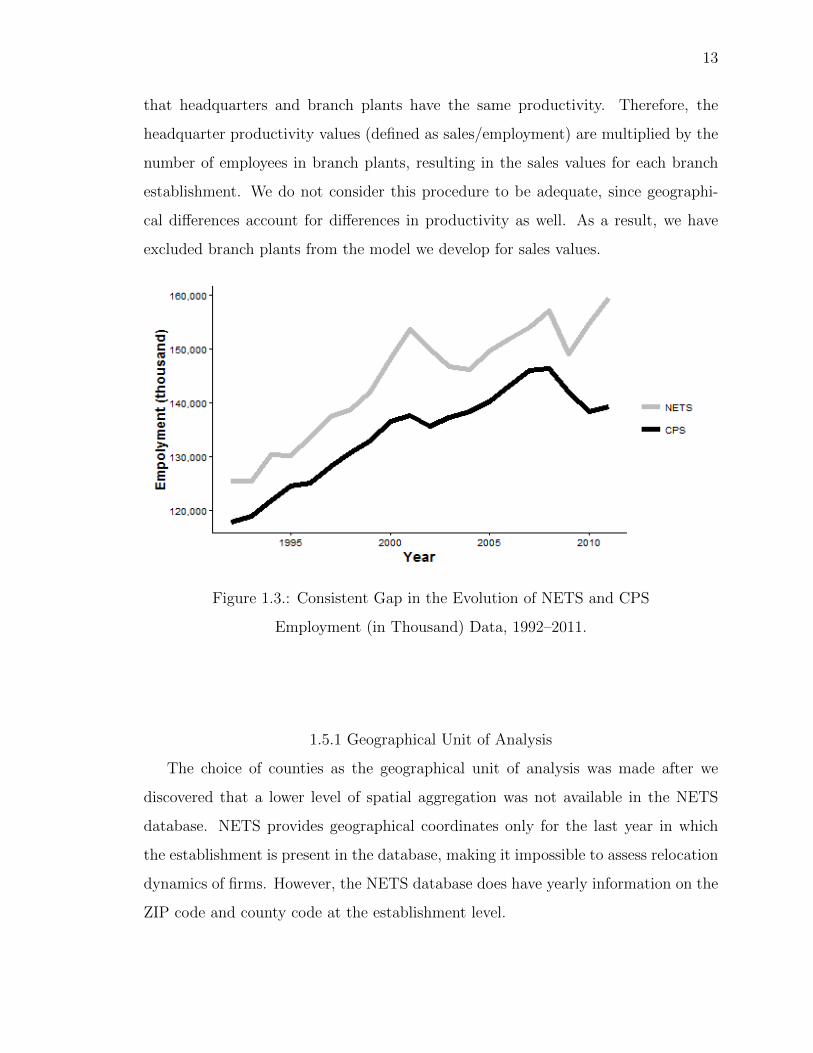
One can see the relationship between NETS employment and the Current Pop-

ulation Survey (CPS)3 employment in Figure 1.3. CPS was chosen due to the fact

it includes self-employment, as does NETS. However, one difference is that NETS

employment is collected at the establishment level, while CPS is a household survey.

Also, NETS is supposedly a population database, whereas CPS is derived from a

sample. Nevertheless, NETS presents larger employment numbers.

NETS does not have the variability one would expect for volatile information such

as sales. When sales are not reported, Walls & Associates estimate the missing value.

Although measurement bias might exist for some firms that do not report sales fig-

ures, we do not see the estimation process as a huge problem. Walls & Associates’

estimation techniques are supposed to decrease bias, because of the use of disaggre-

gate SIC codes and regional proximity matching to attain consistent estimates of

sales values. We can also see that the sales data are also sticky similar to the way in

which employment data are. Again, this is due to the fact of self-reporting and the

estimation process.4 It is also important to notice that the sales of branch establish-

ment are always estimated sales. These estimated sales are based on the assumption

3 CPS data was collected by the Bureau of Labor Statistics and refers to January figures, which isthe same time period in which the NETS snapshots are taken. CPS is, however, seasonally adjusted.4 Several correlation measures were calculated to assess possible sources of bias. Specifically, weestimated the correlation between metropolitan and non-metropolitan areas to see whether differenttrends were present that could be indicative of non-randomness of data. No differences in trend werefound between metropolitan and non-metropolitan areas.

13

that headquarters and branch plants have the same productivity. Therefore, the

headquarter productivity values (defined as sales/employment) are multiplied by the

number of employees in branch plants, resulting in the sales values for each branch

establishment. We do not consider this procedure to be adequate, since geographi-

cal differences account for differences in productivity as well. As a result, we have

excluded branch plants from the model we develop for sales values.

Figure 1.3.: Consistent Gap in the Evolution of NETS and CPS

Employment (in Thousand) Data, 1992–2011.

1.5.1 Geographical Unit of Analysis

The choice of counties as the geographical unit of analysis was made after we

discovered that a lower level of spatial aggregation was not available in the NETS

database. NETS provides geographical coordinates only for the last year in which

the establishment is present in the database, making it impossible to assess relocation

dynamics of firms. However, the NETS database does have yearly information on the

ZIP code and county code at the establishment level.

14

The US has two ZIP code definitions, one used by the United States Postal Service

(USPS), which are used in the NETS database, and another constructed by the

Census Bureau (so-called Zip Code Tabulation Areas, or ZCTAs). The reason why

the Census Bureau had to come up with ZCTAs was that postal ZIP codes change

often, since they are based on optimized mail routes. In this sense, postal ZIP codes

are spatio-temporally very unstable, while ZCTAs have boundaries that are much

more stable.

ZCTAs are constructed based on yearly census blocks. They started being pro-

duced by the Census Bureau in 2000 and by 2010 they were subject to a change in

definition. Theoretically, ZCTA 2000 and ZCTA 2010 are comparable, because they

are built from Census blocks (which are comparable over the years 2000 and 2010). In

practice, however, we would have to decompose both ZCTA into census blocks, match

census blocks and reconstruct a consistent ZCTA for both years. A clear crosswalk

between ZCTA in 2000 and 2010 is not provided by the Census Bureau.

Also, ZCTAs and USPS ZIP codes that share the same 5-digit code may not nec-

essarily cover the same area. The process to develop Postal ZIP code area polygons

is often cited as laborious since these units are not developed and distributed by the

US Postal Service. Rather, private data vendors tend to generate these boundaries.

According to Grubesic and Matisziw (2006) the ZIP code boundaries are created man-

ually after gathering information on residencies and business addresses from USPS.

Then, non-street segments are analyzed. Areas with unclear delineations are identi-

fied and several phone calls are made to area post offices as a checking procedure. It

is therefore unfeasible to produce our own Postal ZIP code.

Fortunately, county boundaries are very stable over the entire period of analysis.

Since we have the county identification number (FIPS) for every establishment, coun-

ties seem to be a natural choice. The drawback of using counties as our geographical

unit of analysis is that their sizes are very different. For larger areas we obviously

loose part of the spatial dynamics.5 Also, counties are not functional regions in an

5 We note, however, that bigger counties have vast uninhabited territories.

15

economic sense, but rather administratively defined areas. On the bright side, coun-

ties are often used for public policy assessment, and we will therefore use counties as

well in our analyses.

1.6 Conclusion

We defined the motivation of the present thesis in Chapter 1. We briefly described

the NETS database, important definitions used in the thesis, and the geographical

unit of analysis (counties). Important areas of regional economics, such as firm de-

mography, location decisions, and agglomeration economies are used extensively in

this thesis.

Chapter 2 deals with the average size of manufacturing firms in the US. We mo-

tivate the study by going back to previous studies on agglomeration, convergence,

and patterns of entry and exit of firms available in the literature of regional eco-

nomics. We use a simple modeling strategy known as Markov chain to describe the

evolution of the average firm size in the manufacturing industry during the period

from 1989–2011. Long run distributions of counties with different firm sizes are found

and reported in the chapter. Moreover, we perform space-time regressions to confirm

some of the results obtained by means of the Markov chain transition probabilities.

Finally, a brief conclusion is at the end.

Chapter 3 looks at patterns of migration of start-up firms. We briefly explain

”nursery city hypothesis”, the theory that motivated the study of start-up relocation.

The theoretical and empirical strategies used to assess the validity of the nursery city

hypothesis are extensively discussed. Results and robustness check are presented as

the main results. Again, we conclude at the end of Chapter 3.

Chapter 4 provides a summary and a general conclusion of the thesis by revising

the hypotheses of Chapter 2 and 3 and presenting the main results. Furthermore, we

contextualize these findings in the public policy debate.

16

CHAPTER 2. SPACE-TIME DYNAMICS OF AVERAGE FIRM SIZE IN

THE US MANUFACTURING INDUSTRY

2.1 Space-Time Dynamics of Establishment Location

2.1.1 Motivation

Firms are attracted by different characteristics of regions when it comes to choos-

ing a location. These characteristics vary from regional amenities, such as temper-

ature and good public transportation, to cost advantages in production (Rosenthal

and Strange, 2003; Glaeser and Kerr, 2009; Arauzo-Carod et al., 2010). Big manu-

facturing plants probably prefer locations close to the input suppliers and with low

land rent cost. Smaller firms might be attracted to areas closer to consumer markets.

The location decisions of firms involve the evaluation of the area’s characteristics that

might help boost profitability, which includes, among other things, the assessment of

other economic agents located there. Hence, the average size of firms in an area is

the outcome of location choices made by companies – both big and small – to locate

in a place. There are a myriad of combinations involving entry rates, exit rates and

migration of firms that might lead to greater or smaller average firm size in a region.

The structure of regions and cities sizes tend not to change in a fast pace (Duranton

and Puga, 1999). Just as city’s size does not change abruptly, the average size of firms

should also not change in a fast pace, unless a positive or negative exogenous shock

affects the region. Some areas have the capabilities to attract big firms with large

scale, while others are a magnet to smaller and innovative companies. Firms assess

17

entry barriers, historical structure of the region, size of regional markets, capacity

to be insulated from external shocks and spatial monopoly opportunities in their

location decision, so the average size of firms depends on these characteristics as

well (Krugman, 1991; Audretsch and Keilbach, 2004; Caves, 2007; Acs et al., 2008;

Neumark et al., 2011).

This chapter describes the regional average size of firms in US counties after

the 1990s, and tests whether path dependency and geographical proximity affect the

probability of a region transitioning from a low average firm size to a large average firm

size structure and vice versa. We hypothesize that a region’s average firm size tends

to stay constant over time, and this constancy is reinforced by the proximity with

regions with the same firm size structure. This chapter also describes and estimates

long-run scenarios of firm size distribution across the United States.

We focus our analysis on the manufacturing industry. The decision to limit the

study to manufacturing sector draws from the evolutionary approach based on the

work of Schumpeter (2013) that also provides a background for the dynamics of new

establishment birth. The evolutionary view argues establishment churn is determined

by the degree of innovative activities, as old traditional sectors are replaced by new

modern ones. Hence, we can also hypothesize that sectors dedicated to innovative

economic activities are more prone to enhance the success of a region due to their

innovative capacity. Historically, manufacturing has a central place in innovation.

Since manufacturing is also largely viewed as a footloose sector, its moving behavior

might affect average firm size of a region too.

Location theory goes back a long way. Since the seminal works of von Thunen

(1826), Weber (1929), and Losch (1954), renewed attention to location factors has

emerged in what is know as the New Economy Geography (Fujita et al., 2001). It

would, however, be misleading to argue that the spatial clustering patterns of firms

have intrigued economists for a long time and many different approaches were devel-

oped to deal with the explanation of location choice (van Wissen, 2002; Pellenbarg

et al., 2002; Rey et al., 2012).

18

There are theoretical milestones on firm location decisions in the economic lit-

erature. Under a profit maximization approach, we hypothesize that firms choose

a location based on expected profits. Therefore, market demand, more productive

labor, and Marshall–Arrow–Romer externalities play a key role in location decisions

(Duranton and Puga, 2001; Brown et al., 2009; Arauzo-Carod et al., 2010).

The idea of modeling the dynamics of establishment location in a space-time

framework comes from the economic growth literature. Many studies have analyzed

the long-run development of economic characteristics, in particular whether there

is convergence in economic variables, for instance, in GDP per capita, income, and

foreign direct investment (Quah, 1996; Bickenbach and Bode, 2003; Rey et al., 2012).

A similarly flavored literature now emerges in firm demography. There is no consensus

in this literature as to why new businesses are established and entrepreneurial activity

grows. However, several studies have found a strong local/regional component to be

important in their analysis (Lee et al., 2004; Glaeser and Kerr, 2009; Glaeser et al.,

2010; Delgado et al., 2010, 2014). The presence of manufacturing, services and/or

natural resource based activities depends on the region and its characteristics. The

reason for firm concentration can also be associated with higher historically present

entrepreneurial activity, barriers to entry and agglomeration externalities associated

with a location.

Agglomeration economies are specific economic advantages coming from spatial

clustering of firms and people that help overcome higher rents and wages for firms in

(growing) urban areas. The micro-foundations of agglomeration economies help us

to connect the location decision of establishments and the locational advantages of a

region. The sources of agglomeration economies are generally grouped in broad cate-

gories, such as localization economies (or Marshallian externalities) and urbanization

economies (Rosenthal and Strange, 2003; Puga, 2010).

As a result of all the abovementioned factors, the size of firms tends to vary across

space. A specific region can attract recently born manufacturing firms; other regions

can be a magnet for manufacturing establishments that are more mature and desire

19

to relocate. In addition, innovative entrepreneurial activity is concentrated in small

innovative establishments which tend to locate in a spatially clustered fashion (Acs

et al., 2008). A higher spatial concentration of the innovative sector fosters entry of

more innovative entrepreneurs. Glaeser et al. (2010) mentions the large entry of small

firms as one of the important causes for the growth of cities.

Several operational measures have been used to capture entrepreneurship. One of

them is small average firm size in a region. However, this measures may identify others

features as well, such as fewer barrier to entry and/or more competitive markets.

Another possible definition, used by Audretsch and Keilbach (2004), is the rate of

new start-ups in the technology sector. This variable is highly correlated with local

success. Kolko and Neumark (2010) try to assess the success of a region by looking

at the changes of employment in regions with greater numbers of locally owned firms,

which is a proxy for local entrepreneurship.

By looking at determinants of local entrepreneurship in a region, Glaeser and Kerr

(2009) find evidence that natural advantages and localized cost measures (natural

resources, transportation cost and labor inputs) are highly correlated with firm entry

patterns. Moreover, a higher number of start-ups is associated with the presence of

industries that hire workers with similar qualifications. Glaeser et al. (2010) argue

that entrepreneurial activity increases in a region with the presence of relevant inputs

– most likely “complex inputs” – like skilled workers.

Relocation is also a type of firm behavior that may affect the number of establish-

ments in a region. In this sense, Delgado et al. (2012) argue industries are affected

by what he calls “cluster environment”.1 Hence, spatial clustering is the result of the

battle between diminishing returns caused by scarcity of economic factors – which

causes migration of capital and workers to places with greater marginal returns – and

the process of agglomeration.

As argued before, a firm will establish in a region if the profit function is higher

than zero after maximization of factors.

1 The authors use a definition created by the US Cluster Mapping Project to define clusters.

20

Formally, as in Rosenthal and Strange (2010):

Π(y, ε) = max(x)a(y)f(x)(1 + ε∗)− c(x) ≥ 0, (2.1)

where y is a vector of local characteristics, x are factors of productions, a is a shifter

and f(x) is the production function with a associated cost c(x). The variable ε∗ is

the critical level of entrance.

Two important aspects must be considered if we want to analyze the evolution

of the average size of manufacturing firms in a given location. The first one is the

spatial scale of the analysis. This involves a crucial ad hoc decision between a higher

or lower spatial resolution. Following Rosenthal and Strange (2003), we could argue

that a higher spatial resolution is preferable, because agglomeration forces attenuate

with geographical distance. However, due to limitations in the available geographical

information2 more aggregate measures must be used.

The second issue is how to compare the number establishments in a region between

different years. The “natural” rate of growth of establishments will mask “real”

changes in firm size if the stock of establishments in the country increases yearly. A

simple measure of “deflation” is to associate the level of employment to the number

of establishments in a region. Mathematically:

LitEit

=

N∑n=1

Lit

N∑n=1

Eit

, (2.2)

where Eit is the number of manufacturing establishment in region i at time t, Lit is

number of employees in manufacturing, and n = 1, ..., N refers to establishment.

The index is adjusted upwards every time a large company with a large number of

employees establishes itself in a region. Thus, a region with higher self employment

2 The database used in this thesis only has the geographical coordinates of establishments at themost recent geographical location, which implies that any approach utilizing grid cells or continuousspace would not capture relocation of establishments.

21

has a smaller index than a region with large establishments. In this sense, the index

of equation (2.2) is the region’s size structure (or we can call it average firm size),

which varies over time.

2.1.2 Method

The dynamics of change in an economic process in a location can be explored in

terms of transition probabilities (Quah, 1996; Rey et al., 2012; Le Gallo, 2004). In

order to assess transition probabilities of for average size of firms classes, we need to

derive a density function of establishment per employees for different time periods,

and compare the evolution of the shape of this distribution between years. After the

characterization of the global distribution of our variable, we can examine the regional

relative movements across distributions by using contingency tables and assuming a

(finite) n-order Markov process to compute transition probabilities. A Markov chain

is a stochastic process in which the probability of a random variable going to state j

in a point of time t+ 1 depends only of the state i at time t (Bickenbach and Bode,

2001). Formally:

P{X(t+ 1) = j|X(t) = i} = pij. (2.3)

The discretization of the data is done as suggested by Quah (1996), dividing the

initial distribution of a variable in classes with a similar number of regions. In our

empirical analysis these classes were constructed by dividing the sample of all regions

in three quantiles.

The evolution of the distribution is represented by the probability matrix M , in

which k is the number of classes provided by the natural breaks (three in our case).

Cell (i, j) in M represents the probability that a region that was in class i at time

t transferred to class j at time t + 1. The frequency of the regions in each class is

represented by the vector Ft (k × 1).

22

The relationship between them is:

Ft+1 = M × Ft, (2.4)

where,

M =

p11 p12 . . . p1N

p21 p22 . . . p2N...

.... . .

...

pN1 pN2 . . . pNN

and

pij ≥ 0,N∑j=1

pij = 1. (2.5)

The transition probability is then given by:

Ft+s = M s × Ft. (2.6)

The (long term) ergodic distribution of F can be found if M is regular (it has no

zero entries), which means the transition probability converges to a limiting matrix

M∗ of rank 1. Therefore, the ergodic distribution F ∗ is characterized by:

F ∗ = M × F ∗. (2.7)

Le Gallo (2004) explains, in this framework each row of M tends to the limiting

distribution as t→∞.

Markov chain transition probabilities are estimated by a Maximum Likelihood

estimator. Bickenbach and Bode (2001) and Bickenbach and Bode (2003) present a

simple optimization for the log-likelihood function used to find unbiased, asymptot-

ically normally distributed transition probabilities.3 If nij is the absolute number of

3 Details about the derivation can be found in Appendix.

23

transitions from state i to state j between t and t+ 1, then:

maxpij

lnL =N∑

i,j=1

nij × ln pij, (2.8)

s.t.∑j

pij = 1, pij ≥ 0, (2.9)

which yields:

pij = nij/∑j

nij. (2.10)

In order to check whether the data generating process conforms with the restric-

tions imposed by the Markov chain theory we need to test the properties of the

Markov process. Two key properties must be tested: the “memoryless” nature of

the time process (the order of time dependence should be zero) and its homogene-

ity in different time periods. We know that the stationarity property is violated by

structural breaks, and by the spatial scale used.4 A higher spatial resolution tends

to capture the heterogeneity of regions better, but at the same time, it increases the

interaction between these areas, implying that the stationary property is harder to

attain.

With that in mind, we will propose a specification for the transition probabilities.

First of all, the order of the Markov chain process must be defined. Bickenbach and

Bode (2003) advises to test primarily lower orders, i.e., order zero against order one,

then first-order Markov chain against second-order, and so forth. The Likelihood

Ratio (LR) test takes the form:

LR(t) = 2T∑t=1

N∑i=1

∑j∈Bi

ni(t)phijpij∼ asyχ2

(N∑i=1

(ai − 1)(bi − 1)

), (2.11)

4 Fingleton (1997) also notes that large one-off shocks are not consistent with transition probabilities.For more details, see Bickenbach and Bode (2003).

24

where phij is a higher order of Markovity, a is the non-zero cells of line j of the

transition probability, and b is the number of non-zero cells of the sum of observations.

We will test time-stationarity by dividing the entire sample (1989–2011) in T time

periods and calculate the respective transition probabilities for these T sub-samples.

The sample is divided considering the exact mid-point of the period, which is also a

recession period between 1989 and 2011. Under the null hypothesis, pij(t) = pij, and

the test is as follows:

LR(t) = 2T∑t=1

N∑i=1

∑j∈Bi

ni(t)pij(t)

pij∼ asyχ2

(N∑i=1

(ai − 1)(bi − 1)

), (2.12)

where pij refers to the entire population and pij(t) refers to the sub-sample. Transition

probabilities with values of zero are excluded from the test statistics. The test has an

asymptotic χ-square distribution with degrees of freedom equal to the positive entries

in the i-th row of the matrix for the entire sample (bi), and the number of sub-samples

(t) in which observations for the i-th row are available (ai), all corrected by the

number of restrictions (Bickenbach and Bode, 2001, 2003). Several other tests can be

developed, but the above tests suffice to check for the formation of clubs of high/low

average firm size in US regions. Geographical concentration of new establishments

in a region can also generate positive externalities and spillovers effects and affect

neighboring regions. In this sense, we should consider the effect that a region with a

high entry of new firms has on its neighbors. The space-time analysis that Rey (2001)

developed, referred to as the “spatial Markov chain”, is suitable for this purpose. The

spatial Markov chain takes the k × k traditional Markov chain and conditions it on

the spatial lag of the surrounding (neighboring) regions in period t− 1. As a result,

we can control for spatial interaction between regions. The k × k × k matrix can be

constructed using the structure of Table 2.1.

If the regional interaction is not important to the dynamics of the transitioning,

then the transition probabilities conditional on spatial lagged class will be similar to

25

those in the non-spatial transition matrix. Hence, the entire spatial matrix will be

equal to a non-spatial matrix transition.

We can formally test whether the transition probability is independent of the

space lags by setting a likelihood test, as in Le Gallo (2004):

LR = 2

{k∑l=1

k∑i=1

j∑l=1

nij(l) log

[pij(l)

pij

]}∼ asyχ2[k(k − 1)2], (2.13)

where k is the number of classes, pij is the non-spatial transition probability, pij(l) is

the conditional probability given state l in period t − 1 and nij(l) is the number of

regions.

With this toolbox in hand we can explore the transition probabilities in US regions.

Table 2.1: The Spatial Lag on which Transition Probabilities are Conditioned.

Lag State t0 Low t1 Medium t1 High t1

Low Low pLowLow|Low pLowMedium|Low pLowHigh|Low

Med pMediumLow|Low pMediumMedium|Low pMediumHigh|Low

High pHighLow|Low pHighMedium|Low pHighHigh|Low

Medium Low pLowLow|Medium pLowMedium|Medium pLowHigh|Medium

Med pMediumLow|Medium pMediumMedium|Medium pMediumHigh|Medium

High pHighLow|Medium pHighMedium|Medium pHighHigh|Medium

High Low pLowLow|High pLowMedium|High pLowHigh|High

Med pMediumLow|High pMediumMedium|High pMediumHigh|High

High pHighLow|High pHighMedium|High pHighHigh|High

2.1.3 Data and Basic Description

Data used in this study goes from 1989 to 2011. The source is the NETS database.

We choose the manufacturing sector (two-digit NAICS code 31–33) to reflect the

26

dynamics of the Schumpeterian innovative process. The lack of information about

the innovative nature of services and the lack of information about Research and

Development and/or value added in each of the manufacturing sectors led us to believe

that studying the whole manufacturing sector would be the best proxy to what we

can call the “innovative sector”.

Hawaii and Alaska are excluded from our database due to remoteness and un-

derstanding that those regions have a rather limited number of firms and they are

not fully integrated with the large consumer markets in the US. Ultimately, we have

3,109 counties to analyze. However, some small counties, such as Loving County,

TX did not have any manufacturing establishment in any of the available years and

were therefore excluded from the database. In addition, there are four counties that

are islands and because of that they do not have a contiguous neighbor. Thus, to be

consistent, we have excluded those as well. In the end, we have 3,094 counties with 23

years of data available. The FIPS code of other excluded counties are 30103, 31007,

31705, 38085, 38087, 46075, 48137, 48261, 48263, 48269, 48301. All of the remaining

counties have a positive average establishment size for at least one year. The basic

statistics can are shown in Table 2.2.

The general trend is towards a lower average establishment size for the analyzed

counties. The median and the mean have decreased from 1989 to 2011. The maximum

value of regional jobs per establishment fluctuated slightly until 2007, but by 2009

the effects of the financial crisis had a big impact on average firm size.

27

Figure 2.1.: Average Firm Size and Number of Establishments for

New, Dying and Migrating Industries in the Manufacturing

Industry, from 1990–2011.

Figure 2.1 shows the variation in average regional firm size over time. We note,

although this is not shown in the Figure, that the trend in the manufacturing sector

is similar to the trend in other sectors: more small firms than large firms entered the

market. Moreover, bigger firms have exited the market more often than small firms.

28

Table 2.2: Evolution of Average Firm Size in the US

Manufacturing Sector, by Quantiles, Between 1989-2011.

Min. 1st Qu. Median Mean 3rd Qu. Max.

Avg. Firm Size 1989 0 10.31 19.55 25.56 33.57 378.65

Avg. Firm Size 1990 0 10.24 19.22 25.10 32.81 382.47

Avg. Firm Size 1991 0 10.14 18.97 24.80 32.66 339.53

Avg. Firm Size 1992 0 10.13 18.69 24.48 32.16 266.40

Avg. Firm Size 1993 0 10.17 18.65 24.35 32.22 345.14

Avg. Firm Size 1994 0 9.92 18.20 23.70 31.16 278.67

Avg. Firm Size 1995 0 9.74 18.33 23.50 31.07 239.17

Avg. Firm Size 1996 0 9.27 17.84 22.69 30.42 201.33

Avg. Firm Size 1997 0 9.26 17.30 22.35 29.43 239.62

Avg. Firm Size 1998 0 9.07 17.34 22.21 29.17 242.69

Avg. Firm Size 1999 0 9.18 17.45 22.49 29.16 475.67

Avg. Firm Size 2000 1 9.22 17.31 22.04 28.97 219.80

Avg. Firm Size 2001 0 8.82 16.74 20.88 27.39 203.00

Avg. Firm Size 2002 0 8.56 15.98 19.98 25.89 203.00

Avg. Firm Size 2003 0 8.34 15.54 19.71 25.34 243.50

Avg. Firm Size 2004 0 8.26 15.27 19.47 25.07 251.00

Avg. Firm Size 2005 0 8.01 14.73 18.62 23.95 204.95

Avg. Firm Size 2006 0 7.83 14.39 18.07 23.36 205.05

Avg. Firm Size 2007 0 7.52 13.82 17.04 21.83 179.26

Avg. Firm Size 2008 0 7.35 12.94 16.03 20.66 178.26

Avg. Firm Size 2009 0 7.65 13.30 16.73 21.74 164.35

Avg. Firm Size 2010 0 7.00 12.20 15.37 19.85 174.94

Avg. Firm Size 2011 0 7.07 12.45 15.72 20.23 199.86

29

Figure 2.2.: Average Size of Manufacturing Firms in the US, in 1989, 2000 and 2011.

Spatially, the same trend can be noticed. By 1989, the East Coast had a high

density of employment per establishment; see Figure 2.2. The West Coast has its

traditional areas of dynamic economic activity, related to urban settlements in Cali-

fornia, Oregon, and Washington. However, even these areas faced a great decrease in

average establishment size from 1989 to 2011. If anything, the distributional statistics

show that a smaller average firm size is a trend in the US during that specific period.

30

2.2 Results

Establishing the order of the Markov chain is a crucial part of obtaining transition

probabilities. In economics, the most popular specification is the first-order Markov

chain, which is used in several applied studies (Quah, 1996; Bickenbach and Bode,

2001, 2003; Le Gallo, 2004; Rey et al., 2012). However, our data may not fit a first-

order Markov chain adequately. In this case, we could have a stochastic process that

is contemporaneous (of order 0), or more time dependent (with an order higher than

1). However, we shall start by fitting the most common model used in economics to

calculate transition probabilities.

Table 2.3 presents the first-order transition probabilities and the limiting vector

for the 1989–2011 period. Low, medium and high classes refer to the first, second

and third terciles of the average size distribution in the year of 1989 used as our

base distribution to assess convergence. As expected, the diagonal of the transition

matrix contains the highest values, which means most of the regions stayed in the

same class of establishment density between 1989 and 2011. Regions where small

establishment are prevalent in 1989 had a more than 95% chance to continue to

have a small average size of firms in 2011. There is a 90% chance of relatively big

average firm size regions to be in the same class between 1989 and 2011, and a 89%

chance for medium average firm size regions not to change class. The likely reason

behind this pattern is the struggle of small manufacturers to grow and expand their

business, while bigger establishments tend to be well established in a region, with

higher persistence than medium size firms (Caves, 2007).5

The second interesting feature of the 1989–2011 transition probabilities is the

comparison between the initial frequency of regions across classes and the long-run

limiting distribution. In 1989, each of the three different classes showed up in almost

one-third of the US regions. In the long run, the limiting distribution shows that

5 Caves (2007) suggests strong presence of barriers of entry and of barriers of exit in some industrialsectors. Mainly, the sunk cost of the capital stock prevents big firms to enter certain markets (anargument that can be extended to have implications for the spatial structure as well), and barriersof exit prevent a firm with low profits to exit the market.

31

regions with low average establishment size would be prevalent (53%), while regions

with high average firm size would become increasingly sparse (14%). One hypothetical

structure for the regions with low average size of manufacturing firms would be to

have a few big establishments surrounded by smaller manufacturing suppliers. Small

establishments in manufacturing are associated with innovation and entrepreneurship

(Glaeser and Kerr, 2009), so these regions might have a high potential for future

growth. For medium average firm size regions the limiting probability is almost the

same as the initial condition.

Table 2.3: Transition Probabilities Based on a First-Order Markov Chain

and the Long-run Limiting Distribution Based on Transition

Probabilities Interaction, 1989–2011.

1989/2011 Low Medium High Initial Dist.

Low 0.9573 0.040 0.0022 0.325

Medium 0.0679 0.893 0.0395 0.332

High 0.0047 0.095 0.9005 0.341

Limiting 0.533 0.325 0.141 1

This simple model needs to fulfill the requisites of the first-order Markov chain

in order to be considered a first-order stochastic process. In our case, a completely

contemporaneous Markov chain is highly unlikely, since location decision are based

on past average profitability, sales volume, and production conditions, among other

factors. In this sense, we test whether the probability of change in the average size of

firms follows a first-order Markov chain as the null hypothesis. The test is constructed

by comparing a first-order Markov chain against a second-order Markov Chain. This

hypothesis is clearly rejected on the basis of an LR-test (LR = 2, 253.19, df = 9,

p-value < 1%). A possible way to attain first-order Markovity is to stretch the time

periods of transition by averaging years. In our case, averaging years would decrease

yearly sample size and it would be unlikely to give any meaningful result. Another

32

option is to increase the spatial resolution in order to capture spatial patterns that

are now hidden under spatial aggregation. This would reflect the potential spatial

heterogeneity of an economic process. As a by-product, we get more reliable estimates

for the Markov chain, but at the same time we increase the probability of violating

Markov properties (Bickenbach and Bode, 2001, 2003).

During the time period of our analysis, the US experienced three economic re-

cessions (1992, 2001 and 2009), according to information of Federal Reserve Bank

(FRED, GDP data). The number of establishments and the level of employment

might have evolved differently because of these external shocks to the local economies,

especially if the establishments were dependent on sectors that were highly affected

by the crises. For that reason, 2001 was chosen as the cutting point to test for time-

independence. The null hypothesis is no differences between the transition probabil-

ities in the period 1989–2001/2001–2011 in comparison to the transition matrix of

1989–2011. The LR-test rejects the null hypothesis (LR = 221.07, df = 18, p-value

< 1%), and hence these matrices are different.

Table 2.4 presents a second-order Markov Chain for the period 1989–2011. The

matrix of transition is now a k×k×k matrix, similar to Table 2.1 . It can be seen that

the diagonals comprise the highest transition probabilities. Thus, it is more likely for

a county to maintain its average firm size than to change it drastically. Vis-a-vis the

first-order transition matrix, the probabilities of staying in the same category, i.e.,

low, medium, or high, conditional on this same category increases for the second-order

case. That is, the diagonal (medium,medium|medium) is greater than the diagonal

(medium,medium) of the first-order Markov chain. Moreover, one can also see that

(medium,medium|medium) is greater than the diagonal (medium,medium|low) of

the second-order Markov chain, which points towards club convergence.

The data generating process of the average size of firms is unknown, so we cannot

know for sure how many time lags influence the average size of manufacturing estab-

lishments in a county. However, the transition probabilities computed along with the

LR-tests reveal a high degree of path dependency. Thus, modeling average manufac-

33

turing firm size using a second-order process seems to capture more variability than

using a simple first-order process.6

Table 2.4: Second-order Transition Probabilities Conditional on t− 2.

1989/2011 Low Medium High

Low

Low 0.969 0.03 0.0018

Medium 0.301 0.69 0.0099

High 0.086 0.10 0.8103

Medium

Low 0.803 0.19 0.0056

Medium 0.060 0.91 0.0299

High 0.003 0.35 0.6435

High

Low 0.8961 0.052 0.052

Medium 0.0253 0.788 0.187

High 0.0046 0.081 0.915

We also find club convergence if we compare the limiting distributions of the

second-order Markov chain. This result is not unexpected, since the second-order

transition probability puts more structure on the transition matrix by trying to cap-

ture path dependency.

Another possible source of disturbance to long-term equilibrium is spatial depen-

dence and spatial heterogeneity. Figure 2.2 shows the map of the contiguous US

territory at the level of counties. We can immediately see the difference between av-

erage firm size on the East and West Coast and average firm size in the manufacturing

belt areas. Krugman (1991) argues the manufacturing belt is the result of a historical

process of spatial concentration that involves transportation costs, demand variables,

and urban areas, so a degree of path dependency may be present here. Space should

therefore also be an important aspect represented in the specification of the Markov

6 Despite the fact that first-order Markov chain is not a likely DGP process and more information canbe attained from higher orders chains, there is a high correlation between the first lag of establishmentfirm size and its contemporaneous value.

34

chain. Specifically, we would like to evaluate how spatially proximate regions move

from different average firm size classes throughout the years, i.e, whether they move

together, stay in the same class or have opposite movements.

Table 2.5: Limiting Distribution of Transition Probability Matrices

Conditional on Lagged Time Structure with the Lag Given in the First

Column.

Limiting Distributions Low Medium High

Low 0.897 0.0898 0.0134

Medium 0.221 0.715 0.0634

High 0.0931 0.266 0.6410

In order to assess the relationship between neighboring regions we can use a mea-

sure of spatial correlation for the 21 years of data available. The result of Moran’s I

tests7 with 999 permutations for the 23 years available are presented in Figure 2.3.

The spatial relationship is estimated by using a queen contiguity weight matrix.8

The queen spatial weights matrix is used despite the evidence of Rosenthal and

Strange (2004) that the extent of spatial spillovers effects due to agglomeration ex-

hibits a strong distance decay pattern. As this is certainly true for agglomeration

process, we are already using a aggregated spatial structure with counties, and the

capacity to capture some of the spatial heterogeneity was therefore already lost. A

distance-based spatial weight structure seems impractical at this level of spatial ag-

gregation, given the bigger-size counties towards the west would require a cut-off

point that makes that too many neighbors will be identified in the eastern part of the

country.

7 For more information about Moran’s I, see Anselin (2013).8 A queen contiguity matrix define neighbors as those with shared border or shared vertex with aregion’s geography.

35

Figure 2.3.: Moran’s I for Average Firm Size of Counties in the US, 1989–2011.

The Global Moran’s Index is positive and statistically significantly different from

zero for all the years. The Moran’s I index is low, as we can see in Figure 2.3. The

spatial Markov chain process will nevertheless be reparameterized in order to evaluate

the dynamics of regional average firm size conditional on the regional average size of

firms of the neighbors. As a result, we can see the influence of the spatial structure

on the Markov chain transition probabilities. Spatial lags are calculated by averaging

the neighbors (given by a queen contiguity weights matrix) and applying the same

class division as used for the non-spatial transition matrix. The spatial transition

probability is a k×k×k matrix where different k×k matrices are computed conditional

on k lag structures. In our case, we have three 3× 3 matrices, as in Table 2.4.

The spatial Markov chain shows some interesting trends. The first trend is that,

in 2011, a county is more likely to stay in the same class it belonged to in 1989, even

conditional on its own spatial lag class. That is to say that the probability to be

in be a county with low average establishment size is higher if conditioned on low

average establishment size of the neighbors. The same is true for medium-medium

and high-high transitions. This result is similar in conclusion to the second-order

36

Markov chain model, showing that both time and space matter in modeling average

regional firm size.

Table 2.6: Spatial Markov Chain Transition Probabilities Conditioned on

Average Neighbor Lag, 1989–2011.

1989/2011 t0/t1 Low Medium High

Lag Low

Low 0.976 0.022 0.0014

Medium 0.117 0.853 0.0294

High 0.028 0.128 0.8441

Lag Medium

Low 0.9406 0.057 0.0024

Medium 0.0636 0.904 0.0327

High 0.0051 0.123 0.8719

Lag High

Low 0.9152 0.079 0.0063

Medium 0.0472 0.888 0.0653

High 0.0019 0.071 0.9266

Another interesting feature relates to the effect on transitions when the neighbors

have a low average establishment size (first 3 × 3 matrix in Table 2.6). When com-

pared to the non-spatial transition probability matrices, the probability that a region

experiences decreasing average establishment size is higher when the neighbors also

have low average establishment size. This may be indicative of spillover effects. At

the same time, it is easier for a region to have a growing average establishment size

if the region has neighbors with high average establishment sizes. Thus, despite the

low value of Moran’s I, the transition probabilities are clearly affected by the spatial

structure.

The question we may pose is whether the spatial matrices are statistically different

from the non-spatial transition matrix. The LR-test rejects the null hypothesis of

equality between the spatial and non-spatial transition matrices (LR = 756.7615,

df = 27, p-value < 1%). Thus, given the results and the test statistic, it is likely

37

that space affects average establishment sizes in regions across the US. However, the

magnitude of Moran’s I is generally very low, closer to a global spatial randomness,

and it poses questioning on how strong is the spatial influence.

Finally, Table 2.7 shows the limiting distribution of the different type regions

conditional on including spatially lagged neighbor information. The results differ

among lags, and they also do not resemble what is found for non-spatial Markov

chains. For instance, 80% of the regions surrounded by counties with low average

establishment sizes will themselves become regions with low average establishment

size in the long run.

Counties with medium establishment size regions as neighbors will tend towards

low establishment size or medium establishment size with almost the same probability,

close to 45%. It will be less likely that regions with such neighbors become regions

with a high average firm size.

It is more likely a region will develop into a region with medium and high av-

erage establishment size when neighbors have a higher number of employees per es-

tablishment. However, probabilities conditioned on the lag ”high” are more evenly

distributed between classes than those probabilities conditioned on the lags ”low”

or ”medium”. A region whose neighbors have a large average size of manufacturing

firms can be seen as a growth pole, or a system of poles as in Lasuen (1973), with dif-

ferently sized manufacturing firms located closely together. The large establishments

in the multi-size pole would influence the expansion in size of smaller manufacturing

establishments.

These results suggest differences between the limiting distribution of non-spatial

and spatial transition probabilities. The non-spatial transitions clearly tend towards

lower average establishment sizes. In the spatial transitions, we see an increasingly

uniform distribution of regions as we condition on higher values of spatial lags. Since

the LR-tests suggest we cannot look at the first-order Markov chain process as the

most likely true data generating process, one can use the spatial transition to take

care of possible spatial heterogeneity in the estimation of transition probabilities.

38

More elaborate regression models can be used to complement the unconditional

regression analyses of average firm size based on Markov chains. These models are

referred to as “spatial process models” or “spatial cross-section models” if they only

consider the spatial dimension (Anselin, 2013), or “spatial panel models” if they

contain both the space and the time dimension (Elhorst, 2014). Implicitly, the spatial

and spatio-temporal processes embedded in these spatial econometric models is also

of the Markov-chain type, utilizing first- or higher-order correlation patterns across

space and time.

Table 2.7: Limiting Distribution of Transition Probability Matrices

Conditioned on Average Neighbor Lag.

Limiting Distributions Low Medium High

Lag Low 0.808 0.155 0.0366

Lag Medium 0.462 0.422 0.116

Lag High 0.229 0.397 0.373

Exploratory, unconditional Markov-type regressions provide an assessment of the

magnitude of the impact of space and time, as well as a robustness check on the

importance of these variables to explain average firm size. One caveat of the un-

conditional Markov chain regression approach is the presence of a high number of

omitted variables that might influence the size of manufacturing plants in a region.

Average firm size is correlated not only with certain characteristics of an area, such as

amenities and infrastructure, but also with the age of firms, the capacity to innovate,

socio-economic variables, and variables related to personal characteristics and man-

agerial capabilities of the entrepreneur (Caves, 2007; Acs et al., 2008). The direction

of the relationship is not always clear and not much has been done in the literature

in terms of model identification in a regression framework. Our goal is not to tackle

these issues directly, but rather to propose a simple correlation assessment of space

and time that might serve as a guide to future work.

39

The Likelihood Ratio tests conduced throughout this chapter point to the rejection

of first-order Markov chain as the preferred modeling strategy to explain or “describe”

the average size of firms at the levels of counties. In addition, the tests clearly show

that higher orders of Markovity and the inclusion of space in the model should be

favored. Hence, we propose three econometric specifications that incorporate space

and time in different ways. We include a measure of space and two time lags are in

the regression models below. We start off by fitting a linear second-order polynomial

expansion on space that includes two lags of the average firm size and the latitude,

longitude, their squares and an interaction term between them. This polynomial

expansion reads as:

Yct = β1Yct−1 + β2Yct−2 + β3Lc + β4LGc + β5L2c + β6LG

2c+

β7(Lc × LGc) + εct,(2.14)

where Y is average establishment size, c is county, t is year, L is latitude, and LG

is longitude of the centroid of the county. The regression is estimated as a pooled

panel, since latitude and longitude are controlling for the spatial distribution of es-

tablishments (henceforth referred to as the “spatial trend”). Time lags examine the

influence of the average size of manufacturing firms (at the county level) at t− 1 and

t− 2 for the average size of manufacturing firms at time t. Results are in Table 2.8.

Based on this regression, we can see the high correlation on the first lag with

contemporaneous average firm size. For every employee per establishment in period

t− 1, we obtain 0.8 employees per establishment in year t. The result is statistically

significant and indicates the high association between average establishment size and

its first lag. The second lag coefficient is only 0.12, meaning there is an impact of 0.12

employee per establishment two years ago for every contemporaneous employee per

establishment. The association is barely significant at 10% level. We can clearly see

that the first order has a strong linear relationship by looking at the the fitted average

establishment size values against the first and second order lags of that variable; see

Figures 2.4 and 2.5.

40

Latitude and longitude are also important to “explain” the variability of firm

size. The further North and East in the United States, the higher the average size of

the manufacturing firm. The square of latitude and longitude show that this rate of

growth marginally decreases. The model has a good fit, but the average firm size of the

geographical neighbors is not yet included explicitly in the model. Moreover, present

and lagged dependent variables may be correlated with unobservable variables, which

would make the ordinary least squares (OLS) estimation inconsistent.

Figure 2.4.: Fitted Average Firm Size Against Average Establishment Size First Lag.

41

Figure 2.5.: Fitted Average Firm Size Against Average Establishment

Size Second Lag.

A simple way to solve the problem is to include spatial fixed effects and take ad-

vantage of the panel structure of the data set. The within transformation is generally

used to sweep the fixed effects out and permit estimation of the parameters of the

regression using transformed variables. By using a fixed effect estimation, all time

invariant variables are also averaged out of the estimation – including the spatial

trend – making the error term not correlated with the independent variables.

However, in our case, the within transformation cannot sweep out all the correla-

tion between the independent variables and the error. This is because the average of

the error term produced by the data transformation in the within estimation is likely

correlated with the average of the lags of the dependent variable used to transform

the time lagged variables in the RHS of the equation9 (Anderson and Hsiao, 1981;

Arellano and Bond, 1991; Baltagi, 2008). We are therefore going to use first-difference

transformations to eliminate the fixed effects and the dynamic panel process devel-

oped by Arellano and Bond (1991) to estimate the parameters of the equation.

9 See Appendix for a econometric assessment.

42

The results are remarkably similar to the pooled model estimated with OLS.

Both time lags are statistically different from zero, and a change of one employee per

establishment in t− 1 leads to an increase of 0.78 employee/establishment in period

t.

Table 2.8: Space-time Regression of the Average Size of Manufacturing

Firms, 1989–2011.

(1) (2) (3)

Coef. S.E. Coef. S.E. Coef M.E. S.E.

Intercept -0.38 2.08

Avg. Firm Sizet−1 0.80** 0.07 0.78** 0.05 0.71** 0.78 0.003

Avg. Firm Sizet−2 0.12* 0.07 0.12** 0.04 0.06** 0.065 0.003

Avg. Firm Size,

Spatial Lag0.09** 0.004

Latitude 0.33** 0.12

Longitude 0.96** 0.26

Latitude2 -0.10** 0.02

Longitude2 -0.26** 0.07

Latitude x Longitude -0.07 0.05

County Fixed Effects No Yes Yes

Adj. R2 0.89

Corr(y,y)2 0.90

LogLik

Note: n = 64, 976. (1) Pooled OLS with White-corrected standard errors. (2) GMM

Dynamic Panel estimated as in Arellano and Bond (1991), where the matrix of in-

struments is based on yi,t−2. (3) Spatial fixed effect panel. Marginal effects (M.E.)

are computed based on a first-order queen contiguity spatial weights matrix.

43

The parameter associated with the two-period time lag is smaller, implying that

a one-employee increase in the average size of firms in period t−2 increases the man-

ufacturing establishment size by 0.12 employees on average in period t. Although we

are more confident that the effects of time lags are being captured by this model than

by the pooled OLS specification, we have not incorporated an explicit spatial process

in the model yet. The spatial Markov chain model shows that the average size of

manufacturing firms at the geographical neighbors impacts the average size of man-

ufacturing firms in a region. The limiting distribution of the transition probabilities

suggests neighboring regions have an impact in the spatial system.

One way to capture this spatial interaction is to use a specification with a spatially

lagged dependent variable. Unobservable variables correlated with the independent

variable can be captured by county fixed effects. The equation to be estimated reads

as:

Yct = β1Yct−1 + β2Yct−2 + β3 + β4WYct + τc + εct, (2.15)

where W is a first-order queen contiguity matrix, and τ are county fixed effects.

A caveat of this model is that we still have to use the within transformation to

eliminate the fixed effects.10 The presence of time lags on the right-hand side of the

equation may render the estimator biased in case fixed-effects are eliminated with the

within transformation (Atems, 2013). The estimated coefficients are very similar to

the estimates obtained by pooled OLS and in the dynamic panel model. Again, both

time lags are statistically different from zero. We proceed and calculate the marginal

effects based on the spatial multiplier. Since the parameter of Wy is small, 0.09, the

total marginal effects are not very different from the estimated coefficients associated

with yt−1 and yt−2.

The results of the panel regressions support the results of the previous Markov

chain analyses. The spatial trend in the pooled model suggests that average firm size

10 Details on the estimation process are provided in Appendix.

44

increases towards the Northeast, which is where the Manufacturing Belt is located.

Moreover, in all the space-time models the one-period lagged regional average size

of manufacturing firms is highly correlated with the contemporaneous firm size. The

two-period lag explains part of the variability as well, but its impact on the contem-

poraneous average size of manufacturing firms is much more limited. The spatial lag

model shows that the spatial autoregressive process is not strong, which is similar to

the conclusion we attained with the spatial Markov chain analysis, but it is never-

theless a relevant component in the explanation of the spatio-temporal distribution

of regional average firm size in the US.

2.3 Conclusion

This chapter investigates the evolution of the dynamics of average regional es-

tablishment size in the manufacturing industry using a Markov chain approach. The

study covers the period from 1989 to 2011. We use counties as the spatial unit of anal-

ysis, knowing that this is not the best spatial resolution for location choice models,

but it is meaningful in terms of public policy.

In order to evaluate the dynamics of average firm size, we fit a first-order Markov

chain process, assuming that this may adequately reflect the true underlying data

generation process of the average size of manufacturing firms. Our hypothesis is that

convergence of manufacturing establishment density will not be attained, since regions

have different firm structure and heterogeneous employment adjustment processes,

leading to different patterns of spatial and temporal dependence. The limiting vector

of transition probabilities points to convergence towards a lower level average firm

size. This idea is consistent with the evolution of the the summary statistics, which

show that counties in the US have been evolving towards dominance of small firms.

However, the assumptions used to fit a first-order Markov chain are not met, which

makes the estimation of long-run transition probabilities likely unreliable. By fitting

a second-order Markov chain, we can see that regions are more inert in a class of firm

45

size the longer in time they have been in that very same class. This points to path

(or time) dependence, a characteristic that is not uncommon in the US (Krugman,

1991).

Our results also suggest this dynamic is not governed strongly by spatial depen-

dence. On the contrary, the Moran’s I statistics are close to 0.04 in several years,

indicating a very low degree of spatial clustering at the county level. However, this is

not to say that space does not matter, since the probability of transition to other firm

size classes may still be influenced by the firm size structure in proximate regions.

Therefore, a spatial Markov chain was estimated using the neighbor’s average firm

size in the manufacturing sector. Transition probabilities were calculated conditional

on these spatially lagged values. We observe that the resulting transition probabili-

ties, conditional on neighbors, are quite different among each other and statistically

different from the non-spatial matrices. In essence, there appears to be a different

convergence pattern depending on the average firm size structure of the neighbors.

Again, a self-re-enforcing pattern of club convergence towards the same class as your

neighbors is an obvious result of our analysis. This is to say that econometric specifi-

cations should account for space-time dynamics to establish meaningful relationships

that might affect entry, exit, persistence and migration of firms.

We estimated space-time regressions to start off the discussion of regression based

studies on average firm size. The regressions confirm the importance of time lags,

since they are highly correlated with the contemporaneous average size of manufac-

turing firms in the United States. The spatial lag coefficient is small, but also highly

significant. The results of the regressions resemble those of the Markov chain models

and are a confirmation of the importance of space and time to firm size.

Planners should also look at the patterns we observe when trying to attract firms

to a county. It is hard to attract big firms to a region when the probability of success

of plants with high employment is low. Focusing on local strengths is the best option

for development of a region, and assessment of firm size structure is a good clue for

the type of company one would like to attract. In addition, the synergies with other

46

counties may as well be a source of concern for the regional planner. The average size

of firms in neighboring regions affects the firm size distribution in the region under

consideration.

Location decision are difficult to assess. In this chapter we have tried to develop

a clearer view on the location preferences of manufacturing firms. The changes in

the density of certain class sizes of manufacturing establishments sheds light on the

process of adjustment of a region over the years. Once more, looking at the ex

post results of location decisions of manufacturing firms may be useful to planners

and researchers who want to tackle a specific problem, such as outsourcing to other

regions or countries. It is clear that regions will not have the same advantages for

every type of industry, but it seems that small manufacturing establishment have

gained increasing importance over the years in United States. So, the analysis of

the joint influence of space and time is paramount to explaining and planning the

spatio-temporal dynamics in the development of the manufacturing industry.

47

CHAPTER 3. DYNAMIC AGGLOMERATION ECONOMIES, START-UPS AND

RELOCATION OF ESTABLISHMENTS

3.1 Nursery City Strategy

This chapter1 tests the validity of the nursery city hypothesis, comprised in a

theory developed by Duranton and Puga (2001). In the article, the authors hypothe-

size an optimal strategy of migration for start-up firms that takes into consideration

the establishment’s product cycle, its production process, the maturing period and

agglomeration economies. The bases of the model are the existence and relevance

of urban and location economies,2 the existence of city developers, free migration

of consumers, optimal investment to keep churn of start-ups, and the assumption

that start-ups do not enter the market with an optimal production process. Start-

ups achieve the ideal production process by experimenting with different mixes of

inputs. Relocation happens every time companies identify this optimal production

process and seek competitive advantages to start mass production (Duranton and

Puga, 2001).

The nursery strategy can be described as the firm’s preference for diversified cities

in the start-up phase. Once a company starts mass production, relocation to other

regions becomes more attractive as specialized cities provide competitive advantages

over diversified cities. As in Jacobs (1969), a diversified region is key to explaining

1 This chapter has been developed in cooperation with Dr. Jos van Ommeren and Dr. Hans Kosterfrom the VU University Amsterdam in the Netherlands, and my advisor at Purdue University.2 The cost of using the same intermediate products diminishes due to more intense usage of interme-diate suppliers. This guarantees that spatial clustering of firms having the same or closely relatedproduction processes in a city or region will decrease the cost of production. Moreover, city size islimited by urban crowding. Specialization advantages are therefore created by location economies.Alternatively, urban economies are created by the diversity in sectoral structure that is typical forlarge urban agglomerations. See Duranton and Puga (2001) and Puga (2010).

48

innovation and the process of product development that takes place in early stages

of the life of companies. Later, specialized regions are important and explain the

relocation of firms, as establishments will seek cost advantages of being close to a

pool of labor, of information exchange with firms in the same sector, and of the usage

of suppliers that cater necessary ingredients for the specialized production process

(Duranton and Puga, 2001; Puga, 2010).

The nursery city model builds heavily on the coexistence of diversified and special-

ized cities/regions. The model guarantees the coexistence of diversified and special-

ized cities in a steady-state equilibrium if five conditions are met: (i) an establishment

must relocate to a more specialized location once it develops the ideal production pro-

cess, (ii) firms start mass production when they achieve the ideal production process,

(iii) firms stay in diversified cities until they find their ideal production process, (iv)

firms constantly try to find the optimal production process, and (v) establishments

do not relocate across specialized cities to find their ideal production process.

Higher profits that can be obtained in mass production lead establishments to end

the “prototype” phase. However, migration is only beneficial once the cost advantages

of producing in a different location are sufficiently large to compensate the costs of

moving. Moreover, some conditions prevent establishments to migrate, even if firms

achieve the ideal production process: (i) the cost of producing in the diversified city

is too low compared to specialized places, (ii) the cost of relocation is too high once

the ideal mix of inputs is found, (iii) the cost of relocation is too low before an ideal

mix of inputs is found (if this is the case, firms may migrate before finishing finding

the ideal production process), and (iv) the advantages obtained from migration to a

specialized city are too small (Duranton and Puga, 2001).

Duranton and Puga (2001) develop the insight that a “balanced urban structure”

is not the one in which cities are equally specialized and diversified. On the contrary,

firms take advantage of an urban structure in which cities/regions foster innovation

and the churning of new ideas (diversified cities), while others raise the profitability

of establishments through specialization. This chapter provides an empirical assess-

49

ment of Duranton and Puga’s theoretical analysis, and tests whether firms that move

are doing so to obtain benefits from specialized areas after they enter the “mass

production” period of their product cycle.

3.2 The Model

3.2.1 The Model Set Up

According to Duranton and Puga (2001) once a start-up initiates mass production,

profitability increases by the relocation to more specialized areas. To assess this

hypothesis, we propose two models based on a random utility maximization (RUM)

framework. RUM models take into account the differences in profitability caused

by different location choices within a spatial system. Hence, firms choose a location

under the assumption of profit maximization behavior.

Let π?isc be the profitability of a start-up i for sector s in region c. This start-up

will randomly try different production processes until it finds the most profitable one.

Each production process has a different cost, and start-ups will benefit from having

contact with firms involved in different production process, because of knowledge

spillovers. Once a firm enters the market, diversity is initially a positive characteristic

of the area surrounding the geographical location of the firm.

Alternatively, a city specialized in one sector does not allow the firm to have

contact with different production processes and, hence, does not help start-ups to

find the optimal product they would like to produce. Instead, a specialized city

provides location externalities that drive profitability up for a specific combination of

inputs. Then, for diversity Dc, specialization Ssc, and a set of input combinations A,

a functional specification for profit is:

π?isc = Sα

?

sc Dβ?

c Aδi . (3.1)

50

At the same time, if πisc represents the profit function of the same establishment

after relocation, then:

πisc = SαscDβcA

δi . (3.2)

Once an establishment finds the optimal production process, the migration to places

where firms can profit from economies of scale and sharing of inputs becomes desirable.

In other words, the establishment needs to relocate to the more specialized place Ssc.

Then diversity of a region, Dc could still have a positive impact on sales through

positive externalities, but not in a sense as crucial as before.

We also know that an establishment will only migrate if profitability of a region

to which it is moving is greater than profitability in the original geographical loca-

tion. Taking logarithms on both sides of equation (3.2) after differentiating between

profitability of movers and stayers (or non-movers) leads to:

log

(πiπ?i

)= log(Ssc)(α− α?) + log(Dc)(β − β?). (3.3)

First-order conditions lead to:

∂log( πiπ?i)

∂log(Ssc)= (α− α?), (3.4)

and:

∂log( πiπ?i)

∂log(Dc)= (β − β?). (3.5)

Equation (3.4) shows the gains of relocation, that is, the cost advantages of being

in a specialized region. Equation (3.5) shows the opposite; that is, the advantages

of of being in a diversified region. We must remember that by the nursery city

theory, Equation (3.4) has a real effect on the decision of moving, while equation

(3.5) represents the willingness to stay in the same region as the establishment initially

chose to locate.

51

By symmetry, we find advantages of staying at the same location as:

∂log(π?i

πi)

∂log(Ssc)= (α? − α), (3.6)

and:

∂log(π?i

πi)

∂log(Dc)= (β? − β), (3.7)

with obvious advantages of diversity depending on the magnitude of the βs.

Figure 3.1.: Benefits of Being a Mover When Mass Production Starts.

It is known that specialization and diversity tend to impact location decisions pos-

itively (Arauzo-Carod et al., 2010). However, using the Duranton and Puga (2001)

argument, the advantages of migration come specifically from specialization, as diver-

sity impacts the decision on where to begin production. Duranton and Puga (2001)

also claim that the nursery city migration strategy is likely to occur in some sectors,

such as certain manufacturing and business services sectors, and not, or only sparsely

in other industries. In particular sectors that can relocate easily (“footloose”) and do

not depend on the availability of natural resources, makes them likely candidates for

migration.

52

The advantages of being a mover by the time an establishment starts mass pro-

duction are represented in Figure 3.1. Similarly, the benefits of being a non-mover are

represented in Figure 3.2. Identification of the nursery city hypothesis comes from

the difference between α and α? and β and β?. We expect α > α? and β? > β for

firms whose behavior is driven by the nursery city strategy.

Figure 3.2.: Benefits of Being a Non-mover when Establishment is in the

Prototype Phase.

3.2.2 Sales Model

In the first specification of a nursery city model we use sales as the dependent

variable. We consider sales as a proxy for profitability.3 Sales can be a surrogate for

profitability once cost saving measures, such as relocation, permits an establishment

to place cheaper products on the market and gain market share. The profitability

of firms increases in case the quantity sold more than compensates the decrease in

3 We could also change perspective and consider the assumption of sales maximization as the mainbehavioral driver of firm behavior Baumol (1958). However, spatial general equilibrium models,such as Duranton and Puga (2001) are based on profit maximization, so we will follow their model.

53

prices.4 Let yit(s,c) denote the total sales of firm i from industry s in county c in year

t. We then estimate the following regression:

log(yit(s,c)) = αritlog(Ssct) + α?(1− rit)log(Ssct)+

+ βritlog(Dct) + β?(1− rit)log(Dct) + εit(s,c),(3.8)

where the question mark indicates firms that have not relocated since their initial

location choice, rit is a dummy variable indicating whether a firm has been relocated

since start-up, Ssct is a index of specialization and Dct is a index of diversification.

The subscript i represents individual firm, s represents sector, c is region, and t is

time. The symbols α, β, α? and β? are parameters to be estimated and εit(s,c) is

an independently and identically distributed error term. We expect that under the

nursery strategy α? < α and β? > β.

The above equation is unlikely to identify causal effects for α and β. First, there

may be general trends in the economy leading to higher or lower sales, so we control

for time fixed effects ζt. The second problem that thwarts identification is the presence

of unobserved location characteristics that may be correlated with specialization or

diversity. For example, larger cities tend to be more diversified (Duranton and Puga,

1999, 2001). We therefore control for density of (manufacturing and business estab-

lishment) workers in the city, denoted by nc, to control for changes in urban costs;

see Behrens and Bougna (2015). We also include location fixed effects, implying that

we identify the effects of specialization and diversity based on temporal variation. In

this way we control at least for all time-invariant unobserved characteristics and for

all unobserved effects that are correlated with overall employment density. A third

problem is that more productive firms select themselves into more productive places

(Behrens and Bougna, 2015). To control for the general level of sales at the life cycle

of the firm and the size of the firm, we control for firm characteristics xit, including

the workforce of the firm, and industrial sector dummies. More importantly, to con-

4 For this to be true, the only assumption needed is that the demand curve exhibits exponentialdecay.

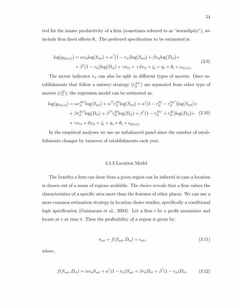
54

trol for the innate productivity of a firm (sometimes referred to as “serendipity”), we

include firm fixed effects θi. The preferred specification to be estimated is:

log(yit(s,c)) = αritlog(Ssct) + α?(1− rit)log(Ssct) + βritlog(Dct)+

+ β?(1− rit)log(Dct) + γnct + +δxit + ζt + ηc + θi + εit(s,c).(3.9)

The mover indicator rit can also be split in different types of movers. Once es-

tablishments that follow a nursery strategy (rNCit ) are separated from other type of

movers (rMit ), the regression model can be estimated as:

log(yit(s,c)) = αrNCit log(Ssct) + α??rMit log(Ssct) + α?(1− rMit − rNCit )log(Ssct)+

+ βrNCit log(Dct) + β??rMit log(Dct) + β?(1− rNCit + rMit )log(Dct)+

+ γnct + δxit + ζt + ηc + θi + εit(s,c).

(3.10)

In the empirical analyses we use an unbalanced panel since the number of estab-

lishments changes by turnover of establishments each year.

3.2.3 Location Model

The benefits a firm can draw from a given region can be inferred in case a location

is chosen out of a menu of regions available. The choice reveals that a firm values the

characteristics of a specific area more than the features of other places. We can use a

more common estimation strategy in location choice studies, specifically a conditional

logit specification (Guimaraes et al., 2003). Let a firm i be a profit maximizer and

locate at c at time t. Then the profitability of a region is given by:

πict = f(Ssct, Dct) + εict, (3.11)

where,

f(Ssct, Dct) = αritSsct + α?(1− rit)Ssct + βritDct + β?(1− rit)Dct. (3.12)

55

We assume εict is distributed according to an Extreme Value Type I distribution.

Then, the probability Πict that a firm i is located in c at time t is:

Πict =ef(Ssct,Dct)∑Kk=1 e

f(Sskt,Dkt), (3.13)

where the establishment can choose from k possible locations. We make the assump-

tion that firms evaluate regions by a set of characteristics common to all locations. If

this is true then equation (3.13) is the conditional logit and we can find the parame-

ters of the model via maximum likelihood (McFadden et al., 1978; Guimaraes et al.,

2003; Schmidheiny and Brulhart, 2011). The log-likelihood function, for c locations,

is given by:

L =C∑c

NclogΠc =C∑c

Ncx′cβ −

C∑c

[Nclog(

C∑c

ex′cβ)

], (3.14)

where x is a set of covariates. This model has a large computational burden when

the number of location choices is big. To decrease this computational intensity, we

can use a random sample of firms, as proposed by McFadden et al. (1978). If the

sample has too many location choices, Guimaraes et al. (2003, 2004) have shown that

the log-likelihood function of the conditional logit model (CLM) has a link with the

log- likelihood function of the Poisson model.5 However, the equivalence of the log-

likelihood of the conditional logit and the Poisson regression only exists if we do not

include establishment-specific characteristics. So, one can estimate a Poisson model

such as:

nscrt = αritSsct + α?(1− rit)Ssct + βritDct + β?(1− rit)Dct + γrct + ζt + ηc + εscrt,

(3.15)

5 See Appendix for a proof.

56

where nscrt is the number of establishment located in county c. We differentiate

between establishments that are migrants r, and that belong to different industrial

sectors, s.

CLM models have limitations since they rest on the assumption of Independence

of Irrelevant Alternatives (IIA). In this context, IIA implies that the characteristics

other than those related the spatial units (in our case, counties) are not relevant for

the location choice of the firm. In this sense, locations must be chosen based on the

comparison of location characteristics after controlling for observable characteristics

of a firm’s “group” characteristics, such as migrants or non-migrants, and industrial

sector. However, we know that unobservable characteristics of a region also have an

impact on location decisions. Hence, Poisson regressions can be altered to include

random and fixed effects (as long as establishment characteristics are left out) and

provide a less computationally intensive model for count data (Guimaraes et al., 2004).

The model is estimate for start-ups that are part of either manufacturing or business

services sector. A different specification might take into account only manufacturing

services, a more standard sector used in location choices.

There are two ways to define movers. A start-up can physically relocate from one

place to another and be considered a mover. A more intuitive way to think of firms

moving is when headquarters open subsidiaries in another location. Although the

headquarters has not physically moved, it certainly can “relocate” to another place,

through the opening of branches. These branches are likely to respond to a parent

firm’s business strategy and for that reason their behavior differs from standalone

firms.

Hence, it may be interesting to think about a more elaborate model that includes

both mover and non-mover start-ups, along with firms that are a result of a strategy

of branching out.

In equation (3.15), all firms that are branches as well as not located in the same re-

gion as the headquarters are defined to be movers. In this way, we can split movers be-

57

tween establishments that move physically and establishments which are subsidiaries.

Our model then assumes the form:

nscmbt = αmitSsct + α??bitSsct + α?(1−mit − bit)Ssct+

+ βmitDct + β??bitDct + β?(1−mit − bit)Dct+

+ γrct + δbct + ζt + ηc + εscmbt,

(3.16)

where bit is a firm that branched out and mit is a firm that physically moved. Again,

in equation (3.15) we define movers as establishments that are branches or estab-

lishments that have physically moved from one region to another. By definition,

bit and mit are mutually exclusive. An establishment is either a branch or a stan-

dalone/headquarter located for the first time in a region. Thus, the model of equation

(3.17) has the same interpretation as equation (3.15). We can split mit between nurs-

ery movers and movers with other strategies:

nscmbt = αmNCit (Ssct) + α??mM

it (Ssct) + α???bitSsct + α?(1−mit − bit)Ssct+

+ βmNCit (Dct) + β??mM

it (Dct) + β???bitDct + β?(1−mit)Dct+

+ γrct + δbct + ζt + ηc + εscmbt.

(3.17)

The nursery city hypothesis is derived from a theory based on the relocation of

firms between cities. Rural areas are not mentioned in the model. However, our

data structure permits only a precise identification of movers between counties.6 As

a result, we will consider an establishment to be moving or branching out when it has

changed location between counties.

3.2.4 Measurement of Specialization and Diversity

Diversity and specialization are two key features of our model specification and we

need an appropriate measurement for them. Several indexes have been proposed to

6 See the data subsection for more details.

58

describe a region as specialized or diversified, and not all of them are equivalent (Du-

ranton and Puga, 1999; Beaudry and Schiffauerova, 2009; Palan, 2010; van Egeraat

et al., 2015). Indexes of specialization can assume various forms, but can broadly be

divided between absolute and relative indexes.

Absolute indexes are those that take the individual sector employment share of

total regional employment as value. For example, an index in which the higher

absolute share of employment is interpreted as a more specialized/diversified region

is an absolute index. The inverse Hirschman–Herfindahl index is an example of such

a category of indexes. Alternatively, a relative specialization index focuses on the

deviation of a region’s employment share in a given sector relative to a benchmark,

e.g., the national employment share of the same industry. Here, the higher the positive

deviation from the benchmark, the more specialized a region is (Palan, 2010).

A crucial aspect of studies on specialization is that the choice of index matters

to the results obtained. A good index has to comply to certain characteristics and

axioms, such as: (i) the order in which one sets up the employment share calcula-

tion should not matter (axiom of anonimity); (ii) exchange of employment from a

more specialized sector to a less specialized sector will imply the region is less ab-

solutely specialized7 (axiom of progressive transfer); (iii) heterogeneity from smaller

sectors contributes less to the index than bigger sector heterogeneity (decomposabil-

ity). Moreover, a good index needs to have bonds; see Palan (2010).

In this study, we use the share of industry employment (measure by 3-digit NAICS)

to total employment in a county as our specialization index (Duranton and Puga,

1999). The index is very simple, but captures the importance of a sector to the

general economy of a county. Formally:

Ssc =EscEc

, (3.18)

7 Until the point that one unit of employment transfer flips the more specialized sector into a lessspecialized sector.

59

where E is employment, s refers to sector, and c is the county. The diversified index

we use is the inverse of Hirschman–Herfindahl index. Mathematically:

IHHc =1∑I

i (Ssc)2, (3.19)

where Sic is the share of employment of a sector in total employment in a region. The

term inside parentheses will be the unit and the IHH index will assume the value of

1 in the case where a region is completely dominated by one sector. Thus, the higher

the index, the more diversified the region.

One potential drawback from the models we propose is the lack of a measure for

agglomeration. Industry concentration that would not be limited by a geographic

frontier is considered a direct measure of agglomeration. Such an indicator could be

calculated with a distance based approach, instead of areal aggregation. Whenever we

use an aggregate measure of specialization and diversity in the econometric specifica-

tion, we lose important information of the interaction between economic forces within

counties (Duranton and Overman, 2005; Briant et al., 2010). We obviously also incur

aggregation bias. Unfortunately, yearly geo-referenced location of establishments is

not available from the NETS database, which renders such a measurement impossible.

3.3 Data

3.3.1 Definition of Variables and Descriptive Statistics

In this subsection we describe the variables used in the regression. County employ-

ment is the sum of employment in the manufacturing and business services industries.

An establishment’s “own employment” is the number of employees in period t for each

establishment i. We do not allow establishments that enter the market with more than

60

300 employees to be considered a start-up,8 since it is likely that these establishments

are a spin-off of other firms. We allow, however, for start-ups to have employment

growth in other subsequent periods, so there are establishments with more than 300

employees in the database.9

Sector fixed effects are based on 3 digits of the NAICS code. Individual fixed effects

are considered to be the unique identifiers for the establishments in the database,

region fixed effects are determined by county FIPS code, and year fixed effects takes

into consideration the 21 years of data available. Alaska and Hawaii were excluded

from the analysis, so 48 states and the District of Columbia are present in our analysis,

as in Chapter 2.

Duranton and Puga (2001) predominantly use the manufacturing sector to assess

empirical evidence of migration patterns that conform with the nursery city strategy.

We would like to extend this framework by introducing not only manufacturing, but

also those sectors that are prone to providing services to manufacturing or to other

businesses. We therefore include in the database all manufacturing sectors (NAICS

code 31–33) and business service sectors (NAICS code 51, 52, and 53). The busi-

ness service sector comprises a broad range of financial activities and communication

industries and around 75% of the database pertains to this category. Descriptive

statistics are presented for the entire population using both business services and

manufacturing industries. We also present basic statistics for the manufacturing sec-

tor only.

The sales model variables are described in Table 3.1. The establishments had, on

average, 3.9 employees, and on average sold $470,000 from 1992 to 2011. The mean

value for diversity is 0.62, which means that most counties are located in places with

a value below the yearly median for diversity, as indicated by the inverse Hirschman–

8 Allowing for 300 employees is a conservative measure. The reason why we are not stricter in ourdefinition of start-up is to allow for establishments that require scale to enter a market.9 As a rule of thumb, we did not allow for an establishment to grow beyond 1,000 employees.Establishments with employees above this number were also excluded from the database.

61

Herfindhal index. Some counties, however, are well above the yearly median, as we

can infer from the maximum value for diversity.

The mean value for specialization is greater than unity. Therefore, on average,

establishments tend to locate in places that are more specialized.10 This fact is

interesting, since based on Duranton and Puga (2001), one could imagine that start-

ups would locate in places that are diversified rather than specialized. The presence of

movers, which are in theory prone to locate in specialized places, is unlikely the cause

of this result, since they only represent 1.95% of the total number of observations in

the database. The largest job market for both manufacturing and business services

is Los Angeles County, in California.

To avoid having to estimate a model with too many observations, a 15% data

sample was obtained for the sales model. The descriptive statistics for the population

and the sample are similar, which indicates that the estimated coefficients can be

generalized to the population.

Descriptive statistics for the location model are presented in Table 3.3.11 The

full population in the location model comprises 28,934,493 establishments, a higher

figure than the sales model due to the inclusion of establishments that branch out to

different locations. Since all establishments that branch out are considered “movers”

in the database, the number of movers increases considerably in the location model:

branching-out movers represent 7.42% of the database and movers, defined as stan-

dalone establishments that migrate to another county, amount to 1.9% of the database.

There are no substantial changes in the descriptive statistics of specialization and

diversity due to the inclusion of branching out. There are still more establishments

located in more specialized areas, as opposed to diversified locations. Compared with

the sales model, the average specialization and diversification are lower once branch-

out establishments are included in the database. The extremes of the specialization

10 Specialization is a characteristic of a sector in a region and therefore comprises all establishments,regardless whether they are start-ups or not.11 If every region had one mover and one non-mover establishment for each sector in every year, wewould have 3,109 counties × 21 years × 36 sectors × 2 (mover and non-movers). However, somecombinations are not present in the data, so the actual database is smaller.

62

index and the diversity index are the same for the location model and the sales model,

since these values do not depend on establishment information. The Poisson model

optimization is more involved and requires smaller sample was required.

Table 3.1: Descriptive Statistics for Variables of the Sales Model for

Manufacturing Industries and Business Services (NAICS 31–33, 51–53).

Sales

(1,000)

Inverse of

HHSpecialization

Employment on

Manuf. And Bus.

Services

Own-

Employment

Population

Min. 0.001 0.269 0.001 65 1

1st Qu. 113 0.417 1.261 87,326 2

Median 175 0.510 1.876 341,777 2

Mean 470 0.622 3.079 738,405 3.879

3rd Qu. 250 0.664 2.947 813,453 3

Max. 2,128,000 22.060 864.611 4,994,121 999

Movers 1.95%

Sample

Min. 0.001 0.269 0.001 131 1

1st Qu. 113 0.417 1.261 87,038 2

Median 175 0.511 1.875 341,471 2

Mean 467 0.622 3.075 736,621 3.892

3rd Qu. 250 0.665 2.946 809,440 3

Max. 2,128,000 22.060 864.611 4, 994,121 950

Movers 1.94%

Note: n = 26, 289, 394 for population and 3, 917, 731 for the sample. Diversity and sp-

cialization are calculated in standard deviations from the median.

63

Thus, a 1% sample was used to estimate the Poisson model with fixed effects. The

diversity and specialization indexes in the population and the sample are fairly similar,

as shown by the descriptive statistics. The number of branch-out establishments in

the sample is higher than in the population, slightly more than 1% point.

Table 3.2: Descriptive Statistics for the Variables of the Sales Model for

Manufacturing Industries (NAICS 31–33).

Sales

(1,000)

Inverse of

HHSpecialization

Employment on

Manuf. And Bus.

Services

Own-

Employment

Population

Min. 0.001 0.2694 0.001 119 1

1st Qu. 78 0.4163 0.97 63,144 1

Median 150 0.5152 1.96 268,052 2

Mean 728 0.6364 3.99 691,336 5.65

3rd Qu. 310 0.6799 3.65 759,389 4

Max. 1,722,000 22.06 864.61 4,994,121 999

Movers 2.80%

Sample

Min. 0.025 0.2694 0.004 187 1

1st Qu. 77 0.4164 0.97 63,634 1

Median 150 0.5144 1.95 268,105 2

Mean 719 0.6364 4.03 686,446 5.624

3rd Qu. 310 0.6791 3.63 758,927 4

Max. 1,722,000 22.06 864.61 4,994,121 990

Movers 2.78%

Note: n = 5, 975, 945 for the population and 896, 137 for the sample. Diversity and sp-

ecialization are calculated in standard deviations from the median.

64

Table 3.4 presents the distribution of movers according to the characteristics of the

counties to which establishments migrate. In the theoretical perspective of Duranton

and Puga (2001), cities are either specialized or diversified.

Table 3.3: Descriptive Statistics for Variables of the Location Model.

Inverse of

HHSpecialization

Population

Min. 0.2643 0.001

1st Qu. 0.4168 1.242

Median 0.5109 1.86

Mean 0.6258 3.098

3rd Qu. 0.6681 2.927

Max. 22.06 864.611

Branchmover 7.42%

Mover 1.94%

Sample

Min. 0.2643 0.0067

1st Qu. 0.4158 1.2452

Median 0.5116 1.8568

Mean 0.6292 3.1662

3rd Qu. 0.6684 2.9114

Max. 22.06 864.611

Branchmover 8.52%

Mover 1.92%

Note: n = 28, 796, 230 for the population.

Diversity and Specialization are calculated

in standard deviations from the median.

65

The matrix represents the combination of diversity and specialization of the county

to which the migrants moved. All 110,140 establishments are represented in the

combination matrix. One can see clearly from the table that the migration of firms

exhibits different preferences for the combination of diversity and specialization. For

instance, the establishment is allocated to the quadrant ++ if the destination county

is more specialized and more diverse than the county of origin. On the other hand,

if an establishment migrated to a less diversified and less specialized county, the

movement is counted in quadrant - - of the matrix. Therefore, each entry of the

matrix represents a combination of diversity and specialization: if the migration path

of a firm is Ssct < Sskt+1, then county k is more specialized than county c and the

firm will be counted as a (+) on the specialization row. On the other hand, if the

movement from the same firm entails that Dct < Dskt+1, it receives a (+) in the

diversity column. The result would be categorized as ++.

Looking at the pattern in which firms migrate, there is not enough evidence to

infer that any of the migratory movements is dominant. Firms that migrate to more

specialized/diversified cities represent almost 27% of the movers. Establishments that

migrated to more specialized and less diverse counties represent 21.4% of all movers,

while firms that move from more specialized to less diverse counties total more than

18.8%. Almost 33% of the movers go to less diversified and specialized places.12

Duranton and Puga (2001) provide evidence that most of the migratory move-

ments in France are from regions in which diversification is above the median to areas

where specialization is above the median. They compare sectors such as R&D, busi-

ness services, textiles, metal products and machinery, among other sectors in order to

find these results. This result provides evidence of the use of the nursery city strat-

egy for these sectors. As we can see from Table 3.5, in column NurseryDP-Movers

Ratio this is the case for start-ups in the US as well. This column shows the ratio

of firms that migrated from above the median diverse counties to above the median

12 All measures of diversity and specialization are normalized by the yearly median in the case ofthe diversity, and by the sector-specific yearly median, in the case of the specialization index.

66

specialized counties divided by the total number of firms that migrated during the

period. The share of nursery city movers is 72%, even higher than the Duranton

and Puga (2001) figures. Sectors such as printing, data processing, real estate and

telecommunications have a nursery city ratio surpassing 80%. The smallest value for

this ratio is for the sector producing wood and furniture products, an industry known

for its concentration in a few regions in the US.

Table 3.4: Number of Migrants Between Different Type of Regions.

Specialization

(+) (-)

Diversity

(+)29,601 20,739

(26.9%) (18.8%)

(-)23,599 36,201

(21.4%) (32.9%)

Note: The matrix describes the num-

ber of migrants that chose the des-

tination county in which diversity

(rows) and specialization (columns)

are above (+) and below the median

(-). All 110,140 migrants are taken

into account.

However, a different story emerges once we look at migration where the county

of origin is above the median specialized and the county of destination is above the

median diversified. This migratory movement can be seen in Table 3.5, in the column

Inverse Nursery DP. The share of establishments that move from counties that are

above the median specialized to counties that are above the median diversified (Inverse

Nursery DP) to total movers (76.1%) is bigger than the share of migrants under

the Duranton and Puga (2001) definition of nursery city. Moreover, most sectors

67

that have high above the median diversification to above the median specialization

migratory ratios, also have large figures in terms of movements between above the

median specialization to above the median diversification counties, as seen in Table

3.5. For instance, the Nursery City DP-Movers ratio for sector 311 is as large as

the Inverse Nursery City DP-Movers ratio, with 59% for the former and 60% for the

latter. This points to evidence that migrating establishments in manufacturing and

in business services in the US have a preference for geographical locations that are

diversified and specialized at the same time.

The intention of the nursery city hypothesis is to differentiate between two types

of location benefits for young firms. One is the interaction with the external business

environment that leads to innovation (optimal production process); the other is the

assessment of characteristics that would cut production costs. Thus, we propose that

the nursery city migrants are those in which the destination county is more specialized

and less diversified than the county of origin. The advantage of this approach is

that it takes into consideration the complex interaction between specialization and

diversification of a region, by treating these variables as a continuum measure rather

than as a binary indicator. In this way, every firm in the database can be a nursery

city migrant, even if the the firm migrates between below the median diversified and

specialized locations.

This strategy is also consistent with the literature on firm migration. If the loca-

tion of firms is bounded by proximity and limited information, then places far away

from the original location of the firms would not be considered as possible destina-

tions (Pellenbarg et al., 2002). As a result, regions that are below the national median

for specialization but closer to the area the establishment is originally located in can

still offer advantages from migration. The only condition is that the destination area

is more specialized than the original location. The assumption of profit maximiza-

tion behavior will still be consistent, although it is constrained by limited spatial

information.

68

Once we look at migrant firms under our definition, nursery city movers drop

in quantity considerably. Using this definition, the ratio of total nursery strategy

movers to total movers drops to 21.4%, as already shown in Table 3.4. Table 3.5

breaks this value up between different sectors. The highly clustered Forest Nurseries

and Gathering of Forest Products sector now has the higher share of nursery movers

in the database, while it had the least using the Duranton and Puga definition.

Insurance carriers and related activities, and printing and related support activities

are a sector in the left-tail of the distribution as far as the share of nursery city movers

is concerned (only 18%). Hence, the choice of how we define movers is crucial, and

in the spirit of the theoretical argument of the original paper, we prefer the latter

definition of nursery city migration.

It should be noted again that in order to compare diversity and specialization, one

needs to normalize these indexes. We normalize by scaling the specialization index

by the annual national median for different sectors. Diversity is normalized by the

annual national median, because it is a measure that pertains to areas, not to sectors.

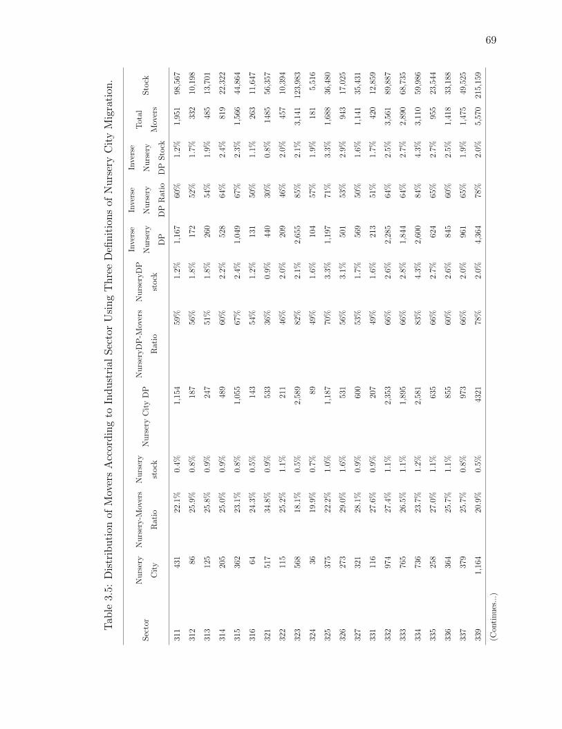
69

Tab

le3.

5:D

istr

ibuti

onof

Mov

ers

Acc

ordin

gto

Indust

rial

Sec

tor

Usi

ng

Thre

eD

efinit

ions

ofN

urs

ery

Cit

yM

igra

tion

.

Sec

tor

Nu

rser

y

Cit

y

Nu

rser

y-M

over

s

Rat

io

Nu

rser

y

stock

Nu

rser

yC

ity

DP

Nu

rser

yD

P-M

over

s

Rat

io

Nu

rser

yD

P

stock

Inve

rse

Nu

rser

y

DP

Inve

rse

Nu

rser

y

DP

Rat

io

Inve

rse

Nu

rser

y

DP

Sto

ck

Tot

al

Mov

ers

Sto

ck

311

431

22.1

%0.

4%1,

154

59%

1.2%

1,16

760

%1.

2%1,

951

98,5

67

312

8625

.9%

0.8%

187

56%

1.8%

172

52%

1.7%

332

10,1

98

313

125

25.8

%0.

9%24

751

%1.

8%26

054

%1.

9%48

513

,701

314

205

25.0

%0.

9%48

960

%2.

2%52

864

%2.

4%81

922

,322

315

362

23.1

%0.

8%1,

055

67%

2.4%

1,04

967

%2.

3%1,

566

44,8

64

316

6424

.3%

0.5%

143

54%

1.2%

131

50%

1.1%

263

11,6

47

321

517

34.8

%0.

9%53

336

%0.

9%44

030

%0.

8%14

8556

,357

322

115

25.2

%1.

1%21

146

%2.

0%20

946

%2.

0%45

710

,394

323

568

18.1

%0.

5%2,

589

82%

2.1%

2,65

585

%2.

1%3,

141

123,

983

324

3619

.9%

0.7%

8949

%1.

6%10

457

%1.

9%18

15,

516

325

375

22.2

%1.

0%1,

187

70%

3.3%

1,19

771

%3.

3%1,

688

36,4

80

326

273

29.0

%1.

6%53

156

%3.

1%50

153

%2.

9%94

317

,025

327

321

28.1

%0.

9%60

053

%1.

7%56

950

%1.

6%1,

141

35,4

31

331

116

27.6

%0.

9%20

749

%1.

6%21

351

%1.

7%42

012

,859

332

974

27.4

%1.

1%2,

353

66%

2.6%

2,28

564

%2.

5%3,

561

89,8

87

333

765

26.5

%1.

1%1,

895

66%

2.8%

1,84

464

%2.

7%2,

890

68,7

35

334

736

23.7

%1.

2%2,

581

83%

4.3%

2,60

084

%4.

3%3,

110

59,9

86

335

258

27.0

%1.

1%63

566

%2.

7%62

465

%2.

7%95

523

,544

336

364

25.7

%1.

1%85

560

%2.

6%84

560

%2.

5%1,

418

33,1

88

337

379

25.7

%0.

8%97

366

%2.

0%96

165

%1.

9%1,

475

49,5

25

339

1,16

420

.9%

0.5%

4321

78%

2.0%

4,36

478

%2.

0%5,

570

215,

159

(Con

tinu

es..

.)

70

conti

nu

ed

Sec

tor

Nu

rser

y

Cit

y

Nu

rser

y-M

over

s

Rat

io

Nu

rser

y

stock

Nu

rser

yC

ity

DP

Nu

rser

yD

P-M

over

s

Rat

io

Nu

rser

yD

P

stock

Inve

rse

Nu

rser

y

DP

Inve

rse

Nu

rser

y

DP

Rat

io

Inve

rse

Nu

rser

y

DP

Sto

ck

Tot

al

Mov

ers

Sto

ck

511

1,10

020

.8%

0.6%

4,26

781

%2.

2%4,

368

83%

2.2%

5,27

819

8,19

7

512

770

18.3

%0.

4%3,

566

85%

1.8%

3,63

086

%1.

8%4,

209

203,

553

515

9619

.6%

0.4%

274

56%

1.2%

292

59%

1.3%

491

23,0

99

517

810

19.9

%0.

3%3,

246

80%

1.3%

3,25

080

%1.

3%4,

063

249,

127

518

1,07

019

.6%

0.8%

4,62

485

%3.

6%4,

675

86%

3.7%

5,46

712

6,87

7

519

6327

.8%

0.3%

105

46%

0.4%

108

48%

0.5%

227

23,9

50

522

1,96

819

.9%

0.5%

6,31

864

%1.

7%6,

536

66%

1.7%

9,87

237

7,21

6

523

1,70

519

.1%

0.2%

7,91

488

%1.

1%7,

929

89%

1.1%

8,94

974

0,70

2

524

1,70

118

.1%

0.4%

7,30

578

%1.

6%7,

275

78%

1.6%

9,37

244

9,07

1

525

236

18.7

%0.

5%1,

071

85%

2.3%

1,07

085

%2.

3%1,

263

45,6

03

531

5,00

321

.9%

0.3%

18,9

6683

%1.

3%18

,831

82%

1.3%

22,8

321,

486,

728

532

806

19.5

%0.

3%3,

061

74%

1.2%

3,08

175

%1.

2%4,

124

261,

868

533

3726

.1%

1.0%

8459

%2.

3%10

272

%2.

8%14

23,

639

Tot

al23

,599

21.4

%0.

5%83

,636

75.9

%1.

6%83

,865

76.1

%1.

6%11

0,14

05,

228,

998

Mig

rant:

nu

rser

yci

ty(m

igra

tion

tom

ore

spec

iali

zed

and

less

div

ersi

fied

cou

nty

),nu

rser

yci

tyD

P(m

igra

tion

from

div

ersi

fied

cou

nty

tosp

ecia

lize

dco

unty

),

and

the

Inve

rse

ofD

P(m

igra

tion

from

spec

iali

zed

tod

iver

sifi

edco

unty

).

71

3.3.2 Data Visualization

Specialization and diversity measured at the level of counties do not reflect the

preferred level of spatial aggregation in the literature. Cities are regarded as the

most interesting and dynamic spatial unit available, because of the high agglomer-

ation of people and businesses on a relatively small area of land. Other studies use

metropolitan areas to grasp the notion of an urbanized space, although in practice

metropolitan areas contain portions of rural areas as well (Abdel-Rahman and Fujita,

1993; Saxenian, 1994; Glaeser et al., 2010).

A glance of the evolution of diversity in US counties is presented in Figure 3.3.

This figure presents the deviations from the mean of the IHH index, as calculated in

equation (3.19), for 1992 and 2011. The first noticeable difference between the initial

and final distribution of diversity across counties is in southern California. In 2011,

IHH values in dynamic regions were closer to the nation’s average than in 1992. The

Midwest is generally considered a non-diversified area, although some small counties

with high IHH are present. Cook County, where the city of Chicago is located, is an

example of such diversified region in the Midwest. The East Coast is also perceived

as a diversified area. Historically, the East Coast has stayed a very diversified area

of the US over a long period of time.

Visualizing specialization in space is more involved than seeing diversity. The

specialization index is computed for 36 sectors based on the 3-digit NAICS code,

which means each county has 36 different measures of specialization. Moreover, the

specialization index, as shown in equation (3.18), is not comparable between differ-

ent industries, unless we normalize the index. However, even when normalized, the

many combinations between specialization in different sectors makes it difficult to

adequately present specialization in a concise map.

One way out of these difficulties of comparability is to utilize a normalized special-

ization index of each sector and compare it to a normalized diversity index. Counting

the number of sectors in which specialization is higher than diversity in each county

provides a summarized view on which regions are specialized rather than diversified.

72

The higher the number presented in Figures 3.4, 3.5, and 3.6 the more specialized the

county is.

Figure 3.3.: Deviations from the Mean on the Diversity Index, for US

Counties in 1992 and 2011.

Three maps provide more details. Figure 3.4 describes how specialized counties

were in 1992. Noticeable differences between the East and West Coast are obvious. In

the West, we notice that the specialization index is greater than the diversity index,

73

on the East Coast more counties with a highly specialized sector are present. This is

particularly true for the manufacturing belt. The middle part of the US is somewhat

in between, with most of the counties with approximately 12 to 16 sectors with higher

values of specialization than diversification.

Skimming through Figure 3.5 and comparing it to the values of 1992, one can

notice more counties became specialized. The lighter gray associated with fewer

specialized sectors on the West Coast in 1992 has turned to a darker grey. Again,

this is consistent with the loss in diversity of that region, as shown in Figure 3.3. More

specialized counties can also be noticed in the middle of the nation, especially in the

area ranging from Texas to Arizona. The East Coast appears to be as specialized as

in 1992.

Figure 3.4.: Count of the Number of Sectors with a Specialization Index

Exceeding the Diversity Index, in 1992.

74

Figure 3.6 refers to 2011. It is interesting to observe the spatial pattern of the

extent of diversity and specialization after the financial crisis of 2008. The crisis

surely impacted the entrance rate of new businesses, as it also caused many others to

go bankrupt, which is evident from layoff statistics and the weakening of the labor

market (Elsby et al., 2010). Geographically, the counties in the heart of the nation

seemed to have faced a decrease in specialization. Despite this fact, comparing both

coastal areas between 2000 and 2011 leads to the same patterns as observed before.



The geographical description of specialization and diversity is important. In more

recent years, county diversity has been falling in comparison to the beginning of the

1990s. At the same time, manufacturing sectors and business services have jointly

gained importance in several counties during the 1990s, which is evident from spe-

cialization indicators that have surpassed the diversity index. This movement was

75

not followed in the 2000s and the likely causes for that are outsourcing, the success of

China in low-technology manufacturing sectors, and the financial crisis. These causes

will not be explored in any detail here.



3.4 Estimation Results

The estimation results for the sales model and the location model are presented

in the following sequence. Table 3.6 shows the sales model when both manufacturing

and business services sectors are included. Table 3.8 also presents the outcomes of

the location model when all sectors are included. Tables 3.7 and 3.9 are the results

for the sales and location model for the manufacturing sector only. The baseline sales

model follows equation (3.9), which includes fixed effects for establishments, years,

76

counties, and industrial sectors. The extensions of the model per equation (3.10)

are next. The fixed effects are included parsimoniously in the sales model, by first

introducing establishment and year fixed effects, then county fixed effects, and finally

industry fixed effects; see columns (1)–(3), respectively. Results of the model that

differentiates nursery city movers from other types of movers are presented in columns

(4)–(6).

The coefficient of diversity for establishments that do not move are expected to be

greater than the coefficient of diversity for movers; see equation (3.4). By symmetry,

movers would benefit from specialization. Again, this comes from the fact that firms

would gain competitiveness by moving to specialized regions at the expense of leaving

more diversified areas.

The dependent variable sales is used to capture advantages of moving. An increase

in sales after migration means firms are more competitive, hence acquiring market

share. Also, the firm that has moved is hypothesized to start mass production, which

implies economies of scale. The baseline results in Table 3.6 indicate that sales are not

impacted significantly by the degree of specialization nor by the degree of diversity of

counties. Estimated coefficients for sector specialization negatively impact sales for

both movers and non-movers in the model, regardless of the inclusion of different fixed

effects. However, this variable is statistically not different from zero for movers, and

only statistically significant at the 10%-level for non-movers. Sales are not impacted

by diversity.

These sales model baseline results reveal a tendency that can be observed across

all the different sales model specifications: the variable that is highly correlated with

sales is the number of employees working in an establishment. Whenever the number

of employees increase by 1%, sales will increase by 0.95%. That is to say that scale

explains greatly the variability in sales in start-up establishments. At the same time,

gains from outside the firm do not have an impact on sales performance. We need to

keep in mind that the nursery city strategy does not relate directly to sales perfor-

77

mance, but would impact it indirectly. However, the baseline model does not tell us

much about this hypothesis.

An improvement in the model would be to differentiate movers between those

establishments following the nursery city strategy (as in equation (3.10)) and those

who follow another strategy for relocation. These models are provided in columns (4),

(5), and (6) of Table 3.8. The estimation results for the above mentioned coefficients

are negative but statistically not different from zero. Again, most of the variation

in sales is explained by the number of employees. The employment-sales elasticity is

robust across several specifications, and has a value of approximately 0.95.

In almost all models, the dummy mover captures the advantages in migration.

It seems to be the case that movers are getting advantages by relocating to a more

suitable geographical location in terms of sales. Local or regional demand is unlikely

to be the explanation for this increase in sales values since not all establishments

included in the database are dependent on local markets. However, if the establish-

ment is part of a big supply chain, migration may increase sales as the start-up is now

geographically closer to its customers. On average, sales figures for movers are 2%

higher than sales of non-movers. The inclusion of more fixed effects does not change

the results. County fixed effects and sector dummies do not affect the magnitude of

the coefficients. One important fixed effect is the fixed effect that controls for un-

observable establishment characteristics, such as managerial proficiency and inherent

quality of the production process. Year fixed effects may also be crucial as it controls

for short-term market conditions. The inclusion of several fixed effects may lead to

over-specification of the model, since not much variation is left.

78

Table 3.6: Regression on the Log of Establishment Sales,

Manufacturing Sectors and Business Services, 1992-2011.

Base Model Nursery City

(1) (2) (3) (4) (5) (6)

Div (mover) -0.004 0.004 0.004

(0.008) (0.01) (0.01)

Spec (mover) -0.0004 −0.006. -0.005

(0.004) (0.004) (0.004)

Div (non-mover) -0.004 -0.002 -0.002 -0.004 -0.002 -0.002

(0.003) (0.004) (0.004) (0.003) (0.005) (0.005)

Spec (non-mover) −0.004. -0.005 −0.004. −0.004. -0.005** -0.005*

(0.001) (0.002) (0.002) (0.002) (0.002) (0.002)

County Emp.

(Bus. Serv. &

Manuf.)

0.0007 0.012** 0.012 0.001 0.012** 0.012

(0.002) (0.011) (0.011) (0.002) (0.011) (0.011)

Firm-Empl. 0.951** 0.951* 0.951** 0.951** 0.951** 0.951**

(0.002) (0.002) (0.002) (0.003) (0.002) (0.003)

Move (1/0) 0.021** 0.02 0.02* 0.02** 0.021** 0.021**

(0.006) (0.007) (0.007) (0.006) (0.007) (0.007)

Div (NC mover) -0.005 0.0154 0.015

(0.016) (0.017) (0.017)

Spec (NC mover) 0.006 -0.003 -0.003

(0.007) (0.007) (0.007)

Div (O. mover) -0.0006 0.002 0.002

(0.009) (0.011) (0.012)

Spec (O. mover) -0.005 −0.009. -0.009

(0.005) (0.005) (0.005)

continued on next page

79

Table 3.6: continued


Establishment Yes Yes Yes Yes Yes Yes

Years Yes Yes Yes Yes Yes Yes

County No Yes Yes No Yes Yes

Industry No No Yes No No Yes

Adj. R2 0.506 0.505 0.505 0.506 0.505 0.505

F -test 112.6** 112.7** 112.7** 112.6** 112.7 ** 112.7**

Note: n = 3,917,731. Diversity and specialization are calculated in deviations

from the median. The symbols **, *, . refer to the 1, 5, and 10% level of signifi-

cance. All variables are in log, except the dummies. Div is diversity and Spec is

specialization. NC refers to nursery city. O. is Other.

Duranton and Puga (2001) focus their analysis in the manufacturing industries.

Once we restrict the sample to the manufacturing sectors and we perform the anal-

ysis only for manufacturing, results change slightly, although the conclusions remain

largely the same. Establishment employment still is a crucial predictor of increase in

sales, with an elasticity of approximately 0.94. The only difference is that being a

mover has no impact on sales in the manufacturing sample. Despite the lack of sta-

tistical significance in most of what we considered to be the key variables for location

decisions, i.e., specialization and diversity, this model is informative in other ways.

It certainly does not tell the nursery city story, as in Duranton and Puga (2001),

but it shows other interesting characteristics. At first glance it seems that sales are

not an adequate operationalization for gains in productivity caused by input sharing.

Sectoral input share acts by driving the input costs down, but it does not necessarily

translate in more sales in dollar values. The size of the company, i.e., the number

of employees is the variable driving the results. This is consistent with other empir-

ical results and common sense (Caves, 2007), since bigger companies will sell more.

80

Sales for footloose companies are not entirely dependent on local market, meaning

it is hard to evaluate migration decisions by this model. Narrowing the sectors used

in the estimation to only manufacturing industries does not have an effect on the

estimation results, and firm employees are still the driver of sales figures.

The fitting of the models is considered high, with above 50% of the variability

being explained by these variables. This points to the direction of own employment

and the mover dummy as important key factors for this model, since they are the

only variables with a high statistical significance. It also means that fixed effects

accounting for non-observables are helping to explain some of the variation.

81

Table 3.7: Regression on the Log of Establishment Sales,

for Manufacturing Sectors only, from 1992-2011 Period.


(1) (2) (3) (4) (5) (6)

Div (mover) 0.035* 0.048* 0.048.

(0.015) (0.026) (0.026)

Spec (mover) 0.005 -0.002 -0.002

(0.005) (0.006) (0.006)

Div (non-mover) 0.007 0.007 0.007 0.007 0.007 0.007

(0.005) (0.006) (0.006) (0.005) (0.007) (0.007)

Spec (non-mover) -0.010** -0.009** -0.009** -0.009** -0.01** -0.01**

(0.002) (0.002) (0.002) (0.002) (0.002) (0.002)

County Emp.

(Bus. Serv. &

Manuf.)

-0.002 0.013 0.013 -0.003 0.013 0.013

(0.003) (0.02) (0.02) (0.004) (0.020) (0.02)

Firm-Empl. 0.938** 0.938** 0.938** 0.938** 0.938* 0.938**

(0.004) (0.004) (0.004) (0.004) (0.004) (0.004)

Move (1/0) -0.006 -0.007 -0.008 -0.004 -0.004 -0.004

(0.009) (0.017) (0.017) (0.009) (0.017) (0.0167)

Div (NC mover) 0.037 0.08. 0.081.

(0.026) (0.0434) (0.043)

Spec (NC mover) 0.0007 -0.013 -0.014

(0.008) (0.011) (0.011)

Div (O. mover) 0.031 0.035 0.036

(0.015) (0.025) (0.025)

Spec (O. mover) 0.009. 0.002 0.001

(0.006) (0.008) (0.008)


82



(1) (2) (3) (4) (5) (6)

Years No Yes Yes No Yes Yes

Industry No Yes Yes No Yes Yes

County No No Yes No No Yes

Adj. R2 0.508 0.504 0.504 0.508 0.504 0.504

F -test 169.6** 168.4** 168.5** 168.5** 168.4** 169.6**

Note: n = 896,137 Diversity and specialization are calculated in deviations from

the median. The symbols **, *, . refer to the 1, 5, and 10% level of significance.

All variables are in log, except the dummies. Div is diversity and Spec is specia-

lization. NC refers to nursery city.

The location models provides more insight into the relevance of the nursery city

strategy. In these models the characteristics of groups of firms (for instance, sector,

mover or non-movers) and the characteristics of the county, such as specialization

and diversity, increase the probability of an establishment choosing a specific location

(McFadden et al., 1978; Guimaraes et al., 2003, 2004).

Similar to before, the columns (1)–(3) of Tables 3.8 and 3.9 present results of the

base models (movers vs. non-movers). Columns (4)–(6) of the tables present the

specification where the behavior of nursery city movers is assessed.

In contradistinction to the sales model, specialization and diversity are statistically

significant in most of the specifications in Table 3.8. Model (1), which does not

include any fixed effects, attributes a large importance to these two indexes. For

instance, start-ups that are in the prototype phase (non-movers) will increase 63%

in a county as diversity increases one standard deviation from the median. Diversity

is still important for start-ups that migrated, as the increase of one deviation from

the median increases the presence of movers in a county by 20%. Therefore, these

83

results are compatible with the nursery city hypothesis. What do not conform to

the Duranton and Puga (2001) model are the results obtained when specialization

increases in the county. Although the interaction between movers and specialization

suggests an increase of 0.01% for the increase of one deviation from the median in the

county specialization, this value is not statistically significantly different from zero.

However, the same increase in specialization would enlarge the presence of non-mover

start-ups in the county by 0.3%. As one can see, diversity increases would drive more

establishments to a county than specialization in this model.

Model (2) includes fixed effects for years and industrial sectors. Although di-

versity still plays a major role in this model, some changes are noteworthy. First,

the magnitude of the coefficients of diversity increases. A more than 37% increase

in migrant establishments opting for a county would be noted if diversity increased

by one standard deviation from the median. This number is 98% for non-mover

start-ups, again confirming the nursery city hypothesis that diversity is more impor-

tant for non-movers. Specialization becomes statistically significant, although with a

smaller magnitude. One standard deviation from the median would increase mover

establishments in a county by 0.5%, and non-mover establishments by 0.7%

Model (3) includes all fixed effects and is our preferred specification among the

baseline models, since it controls for all characteristics that can affect identification.

The fixed effects for counties swipe out the positive effect of the diversity index.

Hence, the diversity index may be picking up some county amenity-type feature in

models (1) and (2) and once we control for unobserved county characteristics, the

effect of diversity disappears. Then, an increase of one standard deviation from the

median in diversity would decrease movers by 83%. At the same time, this increment

in diversity in a county decreases non-migrant start-ups by 26%. This result is at

odds with the theory that states start-ups will have preference for more diversified

regions.

The estimation results show a similar pattern with respect to the introduction of

fixed effects once we explicitly insert nursery city movers into the model. Model (4)

84

has no fixed effects and reveals that diversity increases 62.6% of non-mover establish-

ments in a county with the increase of one standard deviation from the median. At the

same time, diversity increases 5.6% of nursery city movers in a county, a result that

conforms to the nursery strategy theory. Specialization has no effect in the decision

choices since the interaction of the index with nursery city movers and non-movers

is not statistically different from zero. These results change once we include year

and sector fixed effects: specialization becomes statistically significant, affecting the

choice of nursery city movers by 1.2% and non-movers by 0.1% as the index increases

by one standard deviation from the median. The diversity index also affects location

choice of establishments in equation (5), since increasing one standard deviation from

the median in this index increases both start-ups as well as movers by 97% and 11.5%,

respectively. These results are in line with the nursery city hypothesis.

However, the diversity index coefficients turn to negative once we introduce fixed

effects for counties. Although the diversity coefficient of non-mover start-ups is greater

than the value of diversity for nursery city movers, we still have the odd situation in

which positive increments in diversity would drive establishments away from a county.

The literature has been emphatic in estimating positive effects of urbanization

economics on location decisions (Holl, 2004; Manjon-Antolın and Arauzo-Carod, 2011;

Renski, 2011). Only a few contributions have dealt with start-ups and relocation,

and included location fixed effects along with a firm diversity measure. Holl (2004) is

probably the closest we have from a location decision model similar to this study. The

author finds a negative coefficient for ”lack of diversity” (the Hirschman–Herfindhal

index instead of its inverse, as we have used here). Thus, in most studies, unobservable

characteristics of regions and cities are not accounted for. Hence, if we look at the

model without county fixed effects, results are consistent not only with previous

literature, but also with main argument of Duranton and Puga (2001) about the

migration behavior of start-ups.

A feature of this model that can also be explored is the presence of other types

of strategies, such as branching out to to subsidiary establishments. Branches seem

85

to closely follow the behavior of other movers. For instance, in models (3) and (4)

in Table 3.8, the diversity index has positive effects on the presence of branches in

a county, but the impact is not greater than for non-movers. The specialization

index in model (1) is not statistically significant, but specialization has a small and

significant role in attracting more branch establishment to a county when fixed effects

are introduced. These results are not so different from movers who base their behavior

on other strategies.

Another modeling possibility is to restrict the sample to the manufacturing sector

and perform the same analysis based on equation (3.17). The results can be seen

in Table 3.9. Once again, the base model is presented first in columns (1)– (3), and

subsequently in columns (4)– (6) movers are differentiated according to nursery city,

branches and an other strategy.

Table 3.9 shows that the dummy variable mover has gained in importance. In five

out of six specifications, being a mover has a strong positive effect on location choices,

implying that manufacturing firms obtain benefits by relocating from the original

county to another location. The only specification in which this is not true is the

specification where county fixed effects are included in model (6). The magnitude of

the dummy mover is comparable to the benefits obtained by diversity for non-movers

in almost all regressions. The exceptions are regressions (3) and (6) in which inclusion

of location fixed effects changes the sign of the diversity coefficients associated with

stayers and movers.

Benefits of diversity to non-mover start-ups tend to be larger than to movers in

the manufacturing sample. The signs of some coefficients have the wrong direction,

and this is again associated with the introduction of county fixed effects. In general,

there are no benefits for movers that migrate to a more specialized place. However,

we find small benefits associated with start-ups that do not migrate and are located

in a more specialized county. In general, the nursery city strategy is not observed in

the manufacturing sector.

86

Table 3.8: Location Model Based on Poisson Regression,

Manufacturing Sectors and Business Services, 1992-2011


(1) (2) (3) (4) (5) (6)

Div (mover) 0.205** 0.373** -0.830**

(0.031) (0.061) (0.118)

Spec (mover) 0.0001 0.005** 0.005**

(0.001) (0.001) (0.002)

Div (non-mover) 0.636** 0.980** -0.261** 0.626** 0.97** -0.196**

(0.08) (0.132) (0.046) (0.082) (0.126) (0.047)

Spec (non-mover) 0.003* 0.007** 0.008** 0.004. 0.001** 0.012**

(0.001) (0.001) (0.002) (0.002) (0.002) (0.003)

Mover (1/0) 0.151 0.401** 0.087 0.252* 0.542** 0.015.

(0.098) (0.130) (0.154) (0.103) (0.145) (0.169)

Div (NC mover) 0.056** 0.115** -1.07**

(0.019) (0.04) (0.138)

Spec (NC mover) 0.002 0.012** 0.009**

(0.001) (0.001) (0.001)

Div (O. mover) 0.045** 0.0724** -0.923**

(0.015) (0.026) (0.125)

Spec (O. mover) −0.004. 0.009** 0.014

(0.002) (0.003) (0.011)

Div (Bran. mov.) 0.129** 0.004** -0.73**

(0.022) (0.046) (0.115)

Spec (Bran. mov.) 0.001 0.011** 0.005**

(0.001) (0.001) (0.001)




87



(1) (2) (3) (4) (5) (6)


Pseudo R2 0.079 0.216 0.396 0.080 0.211 0.385

Note: n = 137,947 for (4), (5), (6) and 137,330 for (1), (2), (3). Diversity and

Specialization are calculated as deviations from the median and therefore directly

comparable. The symbols **, * and . refer to the 1, 5 and 10% level of significance

. Div is diversity and Spec is specialization. Bran is Branch and O. is other

Diversity and specialization are directly comparable since they are normalized by

the median. In all models, including the full sample as well as the manufacturing

sample, the magnitude of diversity seems to be larger than the magnitude of special-

ization. This means that impacts of diversity on a county’s attractiveness are more

important than sector specialization, a result that is in accordance with most of the

literature on urbanization and specialization economies (Arauzo-Carod et al., 2010).

As a general trend, the results from location models only change when county fixed

effects are included, which seems to amplify the necessity to look at amenity-types

factors driving start-up location rather than directly compare advantages coming from

diversity or specialization.

We can test the magnitude of coefficients is what it is suggested in the nursery

city strategy. In case we reject the hypothesis that diversity impacts the location

decision of non-migrants more than migrants, there is additional evidence that the

nursery city strategy is not a leading behavioral principle. Concurrently, we would

like to see that specialization impacts the behavior of movers more than non-movers.

If this is not the case, there may be other causes to migratory movement, which are

not further explored in this chapter.

88

Table 3.9: Location Model, Manufacturing Sector.


(1) (2) (3) (4) (5) (6)

Div (mover) 0.069** 0.069** -0.638

(0.021) (0.026) (0.147)

Spec (mover) 0.001 0.002** 0.003

(0.0006) (0.0006) (0.002)

Div (non-mov.) 0.397** 0.465** -0.168** 0.41** 0.482** -0.097*

(0.087) (0.104) (0.044) (0.09) (0.114) (0.044)

Spec (non-mov.) 0.006** 0.007** 0.014** 0.002* 0.004** 0.009**

(0.002) (0.002) (0.002) (0.001) (0.001) (0.003)

Mover (1/0) 0.323** 0.492** 0.592** 0.35** 0.472** 0.327

(0.109) (0.14) (0.202) (0.13) (0.160) (0.204)

Div (NC mov.) 0.02* -0.005 -0.498**

(0.01) (0.020) (0.152)

Spec (NC mov.) -0.0001 -0.0002 -0.004

(0.0002) (0.001) (0.003)

Div (O. mov.) 0.02* -0.001 -0.526**

(0.01) (0.015) (0.180)

Spec (O. mov.) -0.0013* -0.006** -0.004

(0.0006) (0.002) (0.004)

Div (Bran.) 0.05** 0.095** -0.450**

(0.01) (0.024) (0.148)

Spec (Bran.) 0.0004 0.002** 0.006**

(0.0004) (0.001) (0.001)





89



(1) (2) (3) (4) (5) (6)

Pseudo R2 0.03 0.05 0.13 0.03 0.06 0.14

Note: n = 52,031 for (4), (5), (6) and 48,661 for (1), (2), (3). Diversity and speci-

alization are calculated as deviations from the median and therefore directly com-

parable. The symbols **, * and . refer to the 1, 5 and 10% level of significance.

Div is diversity and Spec is specialization. O. is other and Bran. is branch, mov.

is mover

As the sales model points to diversity and specialization not having an impact

on establishment sales, we do not report restrictions on the estimated coefficients of

these models. The coefficients are not different from zero and no interesting additional

information was obtained from implementing the restrictions.

Thus, restrictions can be applied to the six sets of regression coefficients estimated

in the location model for manufacturing and business services. First, there are two

restrictions regarding the nursery city strategy, which are applied to the base models

(1)–(3) in Table 3.8: (i) the coefficient of non-movers is smaller than the coefficients

of movers for specialization, and (ii) the coefficient of non-movers is greater than

the coefficients of movers for diversity. We can apply a similar set of restrictions on

the nursery city models (4)–(6): (i) the coefficient of non-movers is greater than the

coefficients of nursery city movers for diversity, and (ii) the coefficient of non-movers

is smaller than the coefficients of nursery city movers for specialization.

Results for the sample that comprises both manufacturing and business services

establishments are presented in Table 3.10. In regression (1), where we do not control

for non-observable characteristics related to time, location, and sector, the one-sided

z-test does not reject the null hypothesis for diversity. The same cannot be said

for specialization, since the hypothesis that specialization impacts movers more than

90

non-movers is rejected at the 5%-level of confidence. Tests performed on models (2)

and (3) lead to the same conclusion. Thus, diversity follows what is expected on the

basis of the nursery city strategy.

Table 3.10: One-sided Test of Restrictions on the Coefficients of Manufacturing and

Business Services Location Model Based on Poisson Regression Results, 1992-2011.


Restriction (1) (2) (3) (4) (5) (6)

Movers < Non-Movers

(Diversity)0.430 0.606 0.569

Movers > Non-Movers

(Specialization)-0.003** -0.002** -0.002*

NC Movers < Non-Movers

(Diversity)0.570 0.854 0.869

NC Movers > Non-Movers

(Specialization)-0.002 0.0016 -0.002

Note: NC refers to nursery city. Numbers in table are the difference in means from

estimated coefficients. ∗∗, ∗ refer to 1%, and 5% significance level.

The same analysis is performed in the in the nursery city model. For these set

of regressions, we would also expect the null hypothesis not to be rejected, since

differentiation between movers were made, with explicit modeling of nursery city

movers. According to the one-sided z-tests, we cannot reject the null hypothesis that

the magnitude of the coefficients are as expected by the theory in any of the models.

These results reinforce the conclusion that differentiating between nursery movers and

other migratory strategies produces a more accurate picture of the migration behavior

of start-up firms. In the Table 3.10, NC refers to nursery city mover. Differences in

means of specific coefficients of the Poisson model are presented in the table.

The same restrictions were tested in the sample with only manufacturing estab-

lishments. In all specifications, the diversity coefficients show a pattern that signals

91

that the manufacturing sector follow the nursery city strategy. However, specializa-

tion does not. This was expected since most of the location choices of movers are not

impacted by specialization in the specification that include only the manufacturing

sector, as can be seen in Table 3.9.

Table 3.11: One-sided Test on Restrictions on the Coefficients of the

Location Model for the Manufacturing Sector.


Restriction (1) (2) (3) (4) (5) (6)

Movers < Non-Movers

(Diversity)0.327 0.395 0.470

Movers > Non-Movers

(Specialization)-0.005** -0.004* -0.011*

NC Mover < Non-Movers

(Diversity)0.327 0.395 0.470

NC Mover > Non-Movers

(Specialization)-0.005** -0.004* -0.011*

Note: NC refers to nursery city. Numbers in table are the difference in means from

estimated coefficients. ∗∗, ∗ refer to 1%, and 5% significance level.

The main results points towards the necessity to look at other characteristics of

regions in order to evaluate the relocation behavior of firms. Diversity and specializa-

tion lead to interesting conclusions when unobservable characteristics are not included

in the model. However, when these firm-specific effects are included, the nursery city

explanation starts to look less appealing, at least for the specifications utilized in this

thesis.

92

3.5 Conclusion

The nursery strategy developed by Duranton and Puga (2001) is one of the finest

theoretical explanations of the behavior of start-up firms in the field of regional eco-

nomics. The theory incorporates product-life cycle characteristics and standard ag-

glomeration theory to explain the relocation behavior of firms, which is an intriguing

topic that has not been subjected to extensive statistical testing.

The main hypothesis of this chapter is that the nursery city strategy may be

observed in the US if we can compare benefits stemming from relocation of start-

ups in industrial sectors prone to migration. The manufacturing sector and business

services are sectors that many regions are interested in having within their boundaries.

In addition, many firms in these sectors can relocate, because they are in principle

footlose.

The best strategy to identify differences in establishments that relocated from a

region as opposed to those that stayed is to estimate the benefits associated with

moving behavior. Under a profit maximization setup, start-ups that are stayers are

drawing advantages of being in the place they originally chose as their production

location. According to Duranton and Puga (2001), this behavior is associated with

the life-cycle of start-ups and their (initial) preference for diversity. Moreover, firms

that relocate are better off in regions that are specialized, since mass production

requires cost minimization in the phase of mass production.

Evaluation of the nursery city strategy is performed for two economic and econo-

metric models, one traditional, aggregate location choice model and one sales model

based on microdata. We argue that identification is obtained by including fixed effects

that would capture possible unobservable characteristics correlated with specializa-

tion and diversity. The caveat of doing so is to exclude other space- or time-constant

predictors of our model, for instance, infrastructure variables or weather. The pre-

ferred specification for both models does not show that the general hypothesis of the

93

nursery city strategy is corroborated. This chapter also identifies nursery movers as

those that migrate to cities that are jointly more specialized and less diversified.

The sales model was found to be inappropriate to deal with location choices.

Mostly, sales are not a good operationalization of productivity differences under profit

maximization. The best predictor for sales increase is the number of employees of

the firm, a somewhat trivial result. Diversity and localization do not statistically

significantly impact sales in any way.

The location model provides interesting results. The nursery city strategy is cor-

roborated for the sample that includes business services and manufacturing industries

until we include county fixed effects in the model. Also, one can conclude that diver-

sity stands out as an important factor in the results, since this index is statistically

significant and large in magnitude. Unfortunately, we observe negative signs on di-

versity coefficients once county fixed effects are included, which makes it difficult to

conclude that nursery city strategy is what governs start-up migration. Location pref-

erences seem to be hardly influenced by other county characteristics, such as county

employment.

These results are somewhat difficult to compare with the literature, as different

techniques and definitions are used to investigate location choice behaviors. As ar-

gued before, the location model estimated through discrete choice models and count

models have been standard in the assessment of firm location. However, the literature

treats agglomeration interchangeably as diversification or specialization. In studies

for the US, agglomeration generally reveals a positive impact on location decisions

(Luger and Shetty, 1985; Head et al., 1995; Coughlin and Segev, 2000; List, 2001;

Gabe, 2003; Guimaraes et al., 2004; Gabe and Bell, 2004; Strauss-Kahn and Vives,

2009). Although rarely assessing both urbanization and specialization together, these

studies provide a consistent finding regarding the sign of the estimated effects of ag-

glomeration economies for location decisions. However, we should note that in the

literature, establishments are taken as homogeneous within a sector. As an alterna-

tive, this chapter evaluated the difference between decisions of start-ups that chose to

94

relocate from where they were originally producing to another geographical location.

Hence, although the methodology used to assess the location choice is the same, the

hypothesis is somewhat different, which might explain the odd signs of some of the

estimated parameters in comparison to the location choice literature.

Studies on start-ups and relocation are scarce compared to empirical studies on

the location decision of sectors, but they have reinforced the idea that agglomera-

tion economies are a significant contributor to firm migration decisions (Holl, 2004;

Arauzo-Carod et al., 2010; Manjon-Antolın and Arauzo-Carod, 2011). This study is

not different: agglomeration forces are indeed important, but not in the same magni-

tude as expected by Duranton and Puga (2001). In conclusion, there is no evidence

that migration from diverse to specialized counties has a significant impact on the

profitability of start-ups once we control for (unobservable) factors that influence

relocation decisions.

95

CHAPTER 4. SUMMARY AND RECOMMENDATIONS

4.1 Revising Hypotheses and Procedures

Two topics related to location decisions of firms, or rather establishments, are

investigated in this thesis. The empirical data we use pertain to the manufacturing

and the business services sectors, in the US, during the last few decades. In Chapter

2, we look at the spatio-temporal distribution of average size of manufacturing firms

in counties in the US between 1990 and 2011. We allow average manufacturing firm

size to belong to classes defined as small, medium, or big1 in a region. We argue

that these three classes or states depend on how long the region has been in a given

state. In addition, we investigate whether the state of average firm size of geographical

neighbors impacts the size structure of firms in a county. The objective of the chapter

is to describe the spatio-temporal evolution of average firm size in the manufacturing

sector at the level of counties.

In Chapter 3, we propose a procedure to test the nursery firm hypothesis. The

nursery city hypothesis argues that start-up establishments prefer diversified cities

at the prototype phase of their product cycle; in other words, immediately after

the establishments enter the market place. Later, when start-ups begin to mass

produce commodities, migration to specialized cities becomes more attractive. We

test whether this hypothesis is valid for business services and for the manufacturing

sector as a whole or only for the manufacturing industry.

The geographical unit of analysis is counties in the US. Many studies have already

stressed the importance of using smaller geographical units in order to adequately

capture spatial heterogeneity (Rosenthal and Strange, 2003; Arauzo-Carod et al.,

1 Defined as the terciles of the distribution of average size of manufacturing firms in 1989.

96

2010). However, in a study across time, spatial units must be stable, or to put it

differently, the geography of the observations has to be constant. In the context of

the National Establishment Time Series (NETS) data we use, we can only attain this

situation for counties.

To test whether average size of manufacturing firms is constant across time and

space, we employ a transition probability technique known as Markov chains. A

Markov chain process is a stochastic process that tests whether a movement between

“regimes” depend on the regimes (or classes) from the past. We test transition proba-

bilities in 21 years with a first-order and a second-order Markov chain. We also employ

a modification of the Markov chain process by conditioning the transition probabil-

ities on the regime that prevails among geographical neighbors. This is known as

a spatial Markov chain process. If the second-order Markov chain and the spatial

Markov chain are different from the first-order process, there is evidence that look-

ing at transition probabilities between classes of regional average firm size without

explicitly considering the time and space dimensions is misleading.

In Chapter 3, we employ a regression-based evaluation of the nursery city hypoth-

esis. In a first step, we define nursery city migrants, since Duranton and Puga (2001)

does not have a definition of how to empirically characterize migratory movements

using both diversity and specialization at the cities of origin and destination. In the

second step, two regression models were proposed to evaluate benefits from being

located in either a diversified or a specialized county. We first estimated a model

that evaluates the impact of diversity and specialization on sales, both for establish-

ments that migrated and those that did not migrate. The second specification uses

the Random Utility Model (RUM) framework to assess the location preferences of

movers and non-movers through a Poisson regression. The probability of a mover

and a non-mover choosing the same location is set to be a function of the pay-offs

of diversity and specialization. The differences between these probabilities are then

evaluated to assess whether the data show a pattern consistent with the nursery city

hypothesis. In the final step, we test whether the coefficients of movers and non-

97

movers are equal both with respect to diversity and specialization, respectively. With

this set of statistical tests, it is possible to assess statistically whether preferences of

movers and non-movers differ.

4.2 Findings for Various Hypotheses

In Chapter 2, the Markov chain models pointed to the importance of evaluating

time and space when assessing the average regional firm size of the manufacturing

industry. Statistical tests on the differences between first-order Markov chain and

second-order Markov chain processes show that useful information can be attained

by introducing more time periods in the Markov chain modeling procedure. At the

same time, despite the fact that spatial correlation is weak, spatial Markov chains

can also provide more information with respect to the transition probabilities between

different size classes as compared to a simpler first-order stochastic process.

In terms of limiting transitions probabilities, all Markov chain models predict

convergence towards a lower regional average size of manufacturing firms, a feature

that was expected given the trends in the descriptive statistics. However, when we

condition the transition probabilities on time and/or space, club convergence is found.

For instance, the probability of a region to be low average firm size in the first-order

Markov chain is lower than the conditional probability of a region to be low average

firm size given it was already low average firm size in the previous period. The same

conclusion is reached when we condition transition probabilities on average firm size

in neighboring regions. If the neighbors are low average firm size, then the probability

of a low average firm size county to continue to be low increases. Table 4.1 concisely

summarizes these results.

Thus, it becomes clear that description of the the regional size structure of man-

ufacturing firms must be done contextualizing it in time and also taking into account

the characteristics of neighboring regions. Also, the conditional transition probabil-

ities show the increasing importance of small establishments in the economy of the

98

US. Geographically, we find that the distribution of small size establishment is more

disperse in recent years. This trend tends to continue in the future, as pointed out

by the findings of conditional and unconditional long run distributions.

Table 4.1: Summary of the Main Limiting Transition Probabilities.

Limiting distributions Low Medium High

First-Order 0.533 0.325 0.141

Condition on time (own-state) 0.897 0.715 0.641

Condition on neighbor (own-state) 0.808 0.422 0.373

Note: The second and third line represent the limiting distribution

of the region’s space and time lag, e.g., the probability of becoming

a region with low average firm size given that neighbors are low

average firm size as well; similarly over time.

In Chapter 3, it has been shown that most of the migration of start-up firms,

belonging to the business services and the manufacturing industry in the US, goes

from above-the-median-specialized places to above-the-median-diversified places. Al-

though Duranton and Puga (2001) treat cities as either specialized or diversified in

their theoretical paper, Chapter 3 shows that this binary classification can be im-

proved if we treat specialization and diversity as continuous variables. Under this

alternative categorization a nursery city migrant is defined as an establishment that

migrates to a county that is jointly less diversified than the original county and more

specialized than the original location. It has been shown that this classification pro-

duces different results as compared to the original Duranton and Puga (2001) paper.

In terms of percentage nursery city movers in relation to total movers we notice an

approximately 75% share of nursery city movers if considered using the definition of

the original paper, but we end up with approximately 21% with utilizing our modified

definition.

99

Both the sales model and the location model are operationalized using two main

specifications: one in which we consider the difference between movers in general and

non-movers, and the other in which nursery city migrants are differentiated from mi-

grants with other moving strategies. Identification of the diversity and specialization

effects is attained by use of fixed effects for establishments (in the sales model only),

as well as year, industry, and county fixed effects. Each one of those sets of fixed

effects controls for a characteristics that can be correlated to diversity and specializa-

tion and thwart identification of the effects we want to estimate. Thus, the preferred

specification contains all the fixed effects.

Benefits from migration come from specialization and benefits from firms that do

not choose to migrate come from diversity. The nursery city hypothesis would be

corroborated if the diversity coefficient of non-movers is greater than the estimated

parameters of movers. At the same time, the coefficient of mover interacted with spe-

cialization should be greater than then the parameter of non-movers interacted with

the same index. All these estimates should be statistically significant and positive.

If these conditions are met, there is evidence that the nursery city strategy is indeed

what governs the location and relocation behavior of start-up firms. However, this is

not what the proposed models show.

Diversity and specialization are not statistically significant in most of the sales

model specifications. The exception is the model for business services and manufac-

turing, in which the coefficient of specialization for non-movers is significant at 5%

confidence level when all fixed effects are included. In the manufacturing-only estab-

lishment sample, this same coefficient is highly significant, but with a negative sign.

Since these results are at odds with most of the literature about location decisions,

it is likely that sales is not capturing location advantages that a county could offer.

Probably, this model captures the scale at which the establishment can produce, as

100

we can see by the importance of the number of employees in explaining the level of

sales.2

Table 4.2 displays in which specification the nursery city is attained in the location

model. We are looking for the situation where all the conditions presented in the table

are true (identified with the word ”Yes”). In that case, the nursery city hypothesis

is valid for manufacturing and business service start-ups migrating between counties

in the US. All the models presented differentiate between nursery migrants and other

types of movers. As one can see, the specification for the entire sample, including year

and industry fixed effects, is the only sample in which the nursery city hypothesis is

not rejected. However, county fixed effects were not included in this specification,

which can cause the error term to be correlated across space with our agglomeration

indexes.

Table 4.2: Summary of the Findings for the Location Model for Two

Different Samples.

Manufacturing Whole Sample

(4) (5) (6) (4) (5) (6)

Diversity NC < Diversity non-mover? Yes Yes Yes Yes Yes Yes

Diversity Coefficient Positive? Yes No No Yes Yes No

Spec. NC >Spec. non-mover? No No No Yes Yes Yes

Spec. Coefficient Positive? No No No Yes Yes Yes

All Statistically significant (1%)? No No No No Yes Yes

Note: NC refers to nursery city Mover.

Our preferred specification does not show evidence that the nursery city hypothesis

holds. It is therefore warranted to state that there is no evidence that establishments

draw benefits from migrating to more specialized and less diversified counties as

2 Alternative specifications with sales per employee as the dependent variable were used as well, butthese alternative definitions do not change the results and conclusions in a meaningful way.

101

compared to the agglomeration externality situation at their original start-up location.

Once we do not condition on unobserved county characteristics, diversity seems to

capture most of the desirable features that would attract start-up firms to a place.

4.3 Can These Results Inform Public Policy?

There are intrinsic differences between geographical locations, be they cities or

counties, that make them more attractive to certain businesses and people (van Wis-

sen, 2002; Hoogstra et al., 2005; Albouy, 2015). Decision makers and planners con-

cerned with the not so prosperous and rather stagnant regions have a strong interest

in trying to escape from the situation where the areas under their administration are

less attractive as compared to other places. Retaining already existent businesses,

fostering entrepreneurship, and attracting new businesses are obvious ways of in-

creasing the prosperity and economic well being of a region. The creation/attraction

of dynamic and innovative firms may function as the exogenous shock needed to re-

establish a regional path of growth. However, it is not always the case that planning

efforts succeed. Thus, having a well-documented assessment of the regional economy

is of paramount importance to any public policy implementation.

Taking the results from this thesis and formulating public policy recommendations

is a difficult task. The two empirical chapters are exercises to understand topics of

firm demography from a regional perspective. Speculating on how our results may be

applicable and useful in a real-world situation is nevertheless useful and interesting.

Chapter 2 has one main conclusion and two recommendations. The main con-

clusion is that average firm size at the level of regions (counties) is rather stable: if

the average regional firm size is divided into a limited number of classes, our results

show that counties tend to remain in the same size class over time (in our case 1989–

2011). However, in the long run, more counties will converge to a lower average firm

size. The recommendations are to consider average firm size in both their spatial and

temporal context. So, in order to attract big firms to a county with a relatively low

102

average firm size, planners could look at counties whose neighbors have a relatively

high average firm size. According to our results, this county has a higher probability

of attracting relatively sizable firms. However, if a region’s neighbors also exhibit a

relatively low average firm size, it is likely that the region’s firm size-structure will

not change much in the long run. Concurrently, planners need to be careful in their

efforts to bring in “big” manufacturing firms to places that are historically endowed

with relatively small firms. It may be that the presence of a new big firm, changes the

region’s production structure in terms of diversity and specialization in a fundamen-

tal way. Chapter 3 demonstrates the relevance of these regional production structure

characteristics.

A careful and thorough assessment of regional characteristics is likely a good start

in terms of planning ahead to identify the type of businesses one would like to retain

or attract, given the capabilities of a county. One of these capabilities is the scale at

which firms can produce, and evaluating the region’s average firm size may be the

first step towards avoiding to spend money from tax payers on enterprises that are

likely to have only a small impact.

At the same time, many regions like to think of themselves as the next Silicon

Valley. Regions try to attract start-ups at a higher rate by creating an environment

that is diversified, where different businesses would likely innovate and create new

jobs. Projects such as Downtown Las Vegas3 try to create this business-friendly

environment through diversification in order to be able to attract new businesses.

However, depending on the level of specialization of a region, new firms seeking cost

saving externalities may prefer to locate in a specialized county.

Chapter 4 has shown that while diversity and specialization of counties are im-

portant to location decisions of start-up firms (regardless of whether the impact is

positive or negative), a planner must think about other types of characteristics of a

region, especially those features that are not directly tangible or quantifiable. This

3 This project focuses on city entrepreneurs by creating conditions for innovative firms to locate indowntown Las Vegas.

103

is even more relevant because the rejection of the nursery citysectionhypothesis when

county characteristics are taken into account points towards the importance of mea-

suring the impact of geographical and social advantages in view of location decisions

of start-up firms. Ignoring these characteristics may lead to the erroneous conclusion

that the diversity of businesses in a city or county is the most important aspect when

it comes to attracting start-ups, when, in reality, entrepreneurs may only be seeking

counties with better weather of a higher quality of life, for example.

4.4 Future Work

Improving the quality of research is a non-linear task. There is always the possi-

bility to test other specifications and add robustness checks. However, sometimes a

step back is more useful.

We can imagine the usefulness of more empirical studies focusing on the regional

average size of manufacturing firms. The components of change of average firm size are

growth in establishment employment, entry, exit, and migration of firms of different

sizes. Thus, studying these variables and how they interact in space is a useful next

step. However, identification of what drives entry, exit and migration is a difficult

task. Looking for programs to attract businesses, e.g., through tax breaks, may be

a good idea to see whether changes in policy effectively change the industrial size

structure of a region. Alternatively, looking at the attractiveness of regions/counties

considering other types of amenities may also be a good idea in approaching the type

of location models presented in Chapter 3. In terms of originality, such research would

probably not be considered to be very innovative, as various authors have analyzed

location choice from different points of view (van Wissen, 2002; Pellenbarg et al.,

2002; Audretsch and Keilbach, 2004; Neumark et al., 2005; Acs et al., 2008; Neumark

et al., 2011).

Expanding Chapter 3 utilizing the same location preference framework as we have

used so far is cumbersome. We have already provided evidence that the nursery city

104

hypothesis can not be corroborated in a regular location model framework, nor with

sales as a proxy for profitability. However, some limitations of the model should be

highlighted. The most obvious is validity, since identification of the model merely

comes from the use of fixed effects accounting for characteristics of the county and

several other unobservable factors. Implicitly, we have left selection of people out

of the model, even although the literature discusses whether firms follow people or

people follow firms (Hoogstra et al., 2005). Moreover, the argument used by Duranton

and Puga (2001) does not touch upon the demographic characteristics of cities. So,

we have implicitly assumed that demographic characteristics of cities are stable over

the life cycle of a firm. Hence, we implicitly assume that these demographic effects

are being picked up by location fixed effects, which is not necessarily true.

Therefore, one option is to include demographic characteristics of cities (or coun-

ties) as a way to explain prevalence of new businesses for particular places. However,

we need to take into account that inverse causation might thwart identification, since

prevalence of start-ups may also bring educated people, more services, etc. to a re-

gion. At the same time, trying to account for amenities is an attractive way to expand

the usefulness and appropriateness of location choice models. The other option is to

change the estimation procedure by explicitly developing a quasi-experiment. The

differentiation between benefits for movers and non-movers resembles a regression

discontinuity design. This is an approach that deserves more and better exploration

in the future, assuming that the right setup to estimate these discontinuities can be

found. Alternatively, a sample selection model utilizing matching techniques to ac-

count for the fact that movers constitute only a small part of sample, could also be

exploited. All these options seem viable, relevant and interesting, but they do require

a complete re-assessment of the sampling procedures and the methodological design,

effectively leading to a new identification strategy. We hope to be able to tackle these

possibilities in the near future.

LIST OF REFERENCES

105

LIST OF REFERENCES

Abdel-Rahman, H. M. and M. Fujita (1993). Specialization and diversification in asystem of cities. Journal of Urban Economics 33 (2), 189–222.

Acs, Z. J., E. L. Glaeser, R. E. Litan, L. Fleming, S. J. Goetz, W. R. Kerr, S. Klepper,S. S. Rosenthal, O. Sorenson, and W. C. Strange (2008). Entrepreneurship and urbansuccess: Toward a policy consensus. Available at SSRN 1092493 .

Albouy, D. (2015). What are cities worth? Land rents, local productivity, and thetotal value of amenities. Review of Economics and Statistics (To be published).

Anas, A. and K. Xiong (2003). Intercity trade and the industrial diversification ofcities. Journal of Urban Economics 54 (2), 258–276.

Anas, A. and K. Xiong (2005). The formation and growth of specialized cities:Efficiency without developers or Malthusian traps. Regional Science and UrbanEconomics 35 (4), 445–470.

Anderson, T. W. and C. Hsiao (1981). Estimation of dynamic models with errorcomponents. Journal of the American Statistical Association 76 (375), 598–606.

Anselin, L. (2013). Spatial econometrics: Methods and models, Volume 4. SpringerScience & Business Media.

Arauzo-Carod, J.-M., D. Liviano-Solis, and M. Manjon-Antolın (2010). Empiricalstudies in industrial location: An assessment of their methods and results. Journalof Regional Science 50 (3), 685–711.

Arbia, G., P. Cella, G. Espa, and D. Giuliani (2015). A micro spatial analysis offirm demography: The case of food stores in the area of Trento (Italy). EmpiricalEconomics 48 (3), 923–937.

Arellano, M. and S. Bond (1991). Some tests of specification for panel data: Montecarlo evidence and an application to employment equations. The Review of EconomicStudies 58 (2), 277–297.

Atems, B. (2013). The spatial dynamics of growth and inequality: Evidence usingUS county-level data. Economics Letters 118 (1), 19–22.

Audretsch, D. and M. Keilbach (2004). Entrepreneurship capital and economicperformance. Regional Studies 38 (8), 949–959.

Audretsch, D. B., E. E. Lehmann, and S. Warning (2005). University spillovers andnew firm location. Research Policy 34 (7), 1113–1122.

106

Audretsch, D. B. and I. Pena-Legazkue (2012). Entrepreneurial activity and re-gional competitiveness: An introduction to the special issue. Small Business Eco-nomics 39 (3), 531–537.

Baltagi, B. (2008). Econometric analysis of panel data, Volume 1. John Wiley &Sons.

Barro, R. J. and X. Sala-i Martin (1992). Convergence. Journal of Political Economy ,223–251.

Baumol, W. J. (1958). On the theory of oligopoly. Economica, 187–198.

Beaudry, C. and A. Schiffauerova (2009). Who’s right, Marshall or Jacobs? Thelocalization versus urbanization debate. Research Policy 38 (2), 318–337.

Behrens, K. and T. Bougna (2015). An anatomy of the geographical concentrationof Canadian manufacturing industries. Regional Science and Urban Economics 51,47–69.

Bickenbach, F. and E. Bode (2001). Markov or not Markov? This should be aquestion. Technical report, Kieler Arbeitspapiere.

Bickenbach, F. and E. Bode (2003). Evaluating the Markov property in studies ofeconomic convergence. International Regional Science Review 26 (3), 363–392.

Briant, A., P.-P. Combes, and M. Lafourcade (2010). Dots to boxes: Do the sizeand shape of spatial units jeopardize economic geography estimations? Journal ofUrban Economics 67 (3), 287–302.

Brown, J. P., R. J. Florax, and K. T. McNamara (2009). Determinants of investmentflows in us manufacturing. The Review of Regional Studies 39 (3), 269–286.

Buss, T. F. (2001). The effect of state tax incentives on economic growth and firmlocation decisions: An overview of the literature. Economic Development Quar-terly 15 (1), 90–105.

Caves, R. E. (2007). In praise of the old IO. International Journal of IndustrialOrganization 25 (1), 1–12.

Coughlin, C. C. and E. Segev (2000). Location determinants of new foreign-ownedmanufacturing plants. Journal of Regional Science 40 (2), 323–351.

Delgado, M., C. Ketels, M. E. Porter, and S. Stern (2012). The determinants ofnational competitiveness. Technical report, National Bureau of Economic Research.

Delgado, M., M. E. Porter, and S. Stern (2010). Clusters and entrepreneurship.Journal of Economic Geography 10 (4), 495–518.

Delgado, M., M. E. Porter, and S. Stern (2014). Clusters, convergence, and economicperformance. Research Policy 43 (10), 1785–1799.

Devereux, M. P., R. Griffith, and H. Simpson (2007). Firm location decisions, re-gional grants and agglomeration externalities. Journal of Public Economics 91 (3),413–435.

107

Dubey, V. (1964). The definition of regional economics. Journal of Regional Sci-ence 5 (2), 25–29.

Duranton, G. and H. G. Overman (2005). Testing for localization using micro-geographic data. Review of Economic Studies , 1077–1106.

Duranton, G. and D. Puga (2001). Nursery cities: Urban diversity, process innova-tion, and the life cycle of products. American Economic Review , 1454–1477.

Duranton, G. and G. Puga (1999). Diversity and specialization in cities: Why,where and when does it matter? Technical report, Centre for Economic PerformanceDiscussion Paper 433, August, London School of Economics and Political Science.

Elhorst, J. P. (2014). Spatial econometrics: From cross-sectional data to spatialpanels. Springer.

Ellison, G., E. L. Glaeser, and W. Kerr (2007). What causes industry agglomera-tion? Evidence from coagglomeration patterns. Technical report, National Bureauof Economic Research.

Elsby, M. W., B. Hobijn, and A. Sahin (2010). The labor market in the greatrecession. Technical report, National Bureau of Economic Research.

Fingleton, B. (1997). Specification and testing of Markov chain models: An ap-plication to convergence in the european union. Oxford Bulletin of Economics andStatistics 59 (3), 385–403.

Fujita, M., P. R. Krugman, and A. Venables (2001). The spatial economy: Cities,regions, and international trade. MIT press.

Gabe, T. (2003). Local industry agglomeration and new business activity. Growthand Change 34 (1), 17–39.

Gabe, T. M. and K. P. Bell (2004). Tradeoffs between local taxes and governmentspending as determinants of business location. Journal of Regional Science 44 (1),21–41.

Gaure, S. (2013). OLS with multiple high dimensional category variables. Compu-tational Statistics & Data Analysis 66, 8–18.

Glaeser, E. L. and W. R. Kerr (2009). Local industrial conditions and entrepreneur-ship: How much of the spatial distribution can we explain? Journal of Economics& Management Strategy 18 (3), 623–663.

Glaeser, E. L., S. S. Rosenthal, and W. C. Strange (2010). Urban economics andentrepreneurship. Journal of Urban Economics 67 (1), 1–14.

Grubesic, T. H. and T. C. Matisziw (2006). On the use of ZIP codes and ZIP codetabulation areas (ZCTAs) for the spatial analysis of epidemiological data. Interna-tional Journal of Health Geographics 5 (1), 58.

Guimaraes, P., O. Figueirdo, and D. Woodward (2003). A tractable approach to thefirm location decision problem. Review of Economics and Statistics 85 (1), 201–204.

108

Guimaraes, P., O. Figueiredo, and D. Woodward (2004). Industrial location model-ing: Extending the random utility framework. Journal of Regional Science 44 (1),1–20.

Guimaraes, P., P. Portugal, et al. (2010). A simple feasible procedure to fit modelswith high-dimensional fixed effects. Stata Journal 10 (4), 628.

Head, K., J. Ries, and D. Swenson (1995). Agglomeration benefits and locationchoice: Evidence from Japanese manufacturing investments in the United States.Journal of International Economics 38 (3), 223–247.

Henderson, J. V. (2003). Marshall’s scale economies. Journal of Urban Eco-nomics 53 (1), 1–28.

Henderson, V. (1997). Externalities and industrial development. Journal of UrbanEconomics 42 (3), 449–470.

Hirschman, A. O. (1958). Interregional and international transmission of economicgrowth. Regional Development and Planning , 623–641.

Holl, A. (2004). Start-ups and relocations: Manufacturing plant location in Portugal.Papers in Regional Science 83 (4), 649–668.

Hoogstra, G., J. Van Dijk, and R. J. Florax (2005). Do jobs follow people or peoplefollow jobs? A meta-analysis of Carlino–Mills studies. Louvain-la-Neuve: EuropeanRegional Science Association (ERSA).

Isard, W. (1956). Regional science, the concept of region, and regional structure.Papers in Regional Science 2 (1), 13–26.

Isard, W. (1960). Methods of regional analysis. Ripol Klassik.

Jacobs, J. (1969). Strategies for helping cities. The American Economic Review ,652–656.

Jarmin, R. S. and J. Miranda (2002). The longitudinal business database. Availableat SSRN 2128793 .

Kolko, J. and D. Neumark (2010). Does local business ownership insulate cities fromeconomic shocks? Journal of Urban Economics 67 (1), 103–115.

Krugman, P. (1991). History and industry location: The case of the manufacturingbelt. The American Economic Review , 80–83.

Lasuen, J. R. (1973). Urbanization and development - the temporal interactionbetween geographical and sectoral clusters. Urban Studies 10 (2), 163–188.

Le Gallo, J. (2004). Space-time analysis of GDP disparities among European regions:A Markov chains approach. International Regional Science Review 27 (2), 138–163.

Lee, S. Y., R. Florida, and Z. Acs (2004). Creativity and entrepreneurship: Aregional analysis of new firm formation. Regional Studies 38 (8), 879–891.

List, J. A. (2001). US county-level determinants of inbound FDI: Evidence from atwo-step modified count data model. International Journal of Industrial Organiza-tion 19 (6), 953–973.

109

Losch, A. (1954). Economics of location. Yale University Press.

Lovell, M. C. (2008). A simple proof of the FWL theorem. The Journal of EconomicEducation 39 (1), 88–91.

Luger, M. I. and S. Shetty (1985). Determinants of foreign plant start-ups in theUnited States: Lessons for policymakers in the Southeast. Vand. J. Transnat’l L. 18,223.

Manjon-Antolın, M. C. and J.-M. Arauzo-Carod (2011). Locations and relocations:Determinants, modelling, and interrelations. The Annals of Regional Science 47 (1),131–146.

Marshall, A. (1890). Principles of political economy. Maxmillan, New York.

McFadden, D. et al. (1978). Modelling the choice of residential location. Institute ofTransportation Studies, University of California.

Millo, G., G. Piras, et al. (2012). splm: Spatial panel data models in R. Journal ofStatistical Software 47 (1), 1–38.

Neumark, D., B. Wall, and J. Zhang (2011). Do small businesses create more jobs?New evidence for the United States from the National Establishment Time Series.The Review of Economics and Statistics 93 (1), 16–29.

Neumark, D., J. Zhang, and B. Wall (2005). Employment dynamics and businessrelocation: New evidence from the National Establishment Time Series. Technicalreport, National Bureau of Economic Research.

Palan, N. (2010). Measurement of specialization–the choice of indices. Technicalreport, FIW.

Pellenbarg, P. H., L. J. Van Wissen, and J. Van Dijk (2002). Firm migration.Industrial Location Economics , 110.

Perloff, H. S. (1957). Regional studies at US universities: A survey of regionallyoriented research and graduate education activities. Resources for the Future.

Perroux, F. (1955). A note on the notion of growth pole. Applied Economy 1 (2),307–320.

Puga, D. (2010). The magnitude and causes of agglomeration economies. Journalof Regional Science 50 (1), 203–219.

Quah, D. T. (1996). Empirics for economic growth and convergence. EuropeanEconomic Review 40 (6), 1353–1375.

Renski, H. (2011). External economies of localization, urbanization and industrialdiversity and new firm survival. Papers in Regional Science 90 (3), 473–502.

Rey, S. J. (2001). Spatial empirics for economic growth and convergence. Geograph-ical Analysis 33 (3), 195–214.

Rey, S. J., E. A. Mack, and J. Koschinsky (2012). Exploratory space-time analysisof burglary patterns. Journal of Quantitative Criminology 28 (3), 509–531.

110

Rosenthal, S. S. and W. C. Strange (2003). Geography, industrial organization, andagglomeration. Review of Economics and Statistics 85 (2), 377–393.

Rosenthal, S. S. and W. C. Strange (2004). Evidence on the nature and sources ofagglomeration economies. Handbook of Regional and Urban Economics 4, 2119–2171.

Rosenthal, S. S. and W. C. Strange (2010). Small establishments/big effects: Ag-glomeration, industrial organization and entrepreneurship. In Agglomeration Eco-nomics, pp. 277–302. University of Chicago Press.

Saxenian, A. (1994). Inside-out: Regional networks and industrial adaptation insilicon valley and route 128. Cityscape 2 (2), 41–60.

Schmidheiny, K. and M. Brulhart (2011). On the equivalence of location choice mod-els: Conditional logit, nested logit and poisson. Journal of Urban Economics 69 (2),214–222.

Schumpeter, J. A. (2013). Capitalism, socialism and democracy. Routledge.

Shalizi, C. (2009). Note: Maximum likelihood estimation for Markov chains. Coursematerial.

Spilerman, S. (1972). The analysis of mobility processes by the introduction ofindependent variables into a Markov chain. American Sociological Review , 277–294.

Strauss-Kahn, V. and X. Vives (2009). Why and where do headquarters move?Regional Science and Urban Economics 39 (2), 168–186.

van Egeraat, C., E. Morgenroth, R. Kroes, D. Curran, and J. Gleeson (2015). Ameasure for identifying substantial geographic concentrations. Technical report,University Library of Munich, Germany.

van Wissen, L. J. (2002). Demography of the firm: A useful metaphor? EuropeanJournal of Population/Revue Europeenne de Demographie 18 (3), 263–279.

Walls, D. W. (2007). National Establishment Time Series database c©: Dataoverview. In 2007 Kauffman Symposium on Entrepreneurship and Innovation Data.

Weber, A. (1929). Theory of the location of industries [translated by CJ Friedrichfrom Webers 1909 book]. Chicago: The University of Chicago Press.

APPENDIX

111

APPENDIX: ECONOMETRIC DETAILS

First, I want to derive the maximum likelihood estimation for the time discrete

Markov chain. This section is based largely on Shalizi (2009). We want to derive a

maximum likelihood estimator to fit a m state Markov chain. Each entry of matrix,

pij will be a probability to transition from state i to state j. Thus,

pij = Pr(Xt+1 = j|Xt = i). (A.1)

Although we do not observe the true DGP of the random variable Xn1 , xn1 , we can

hypothesize the likelihood of the realization of the data to equal:

Pr(Xn1 = xn1 ) = Pr(X1 = x1)

n∏t=2

Pr(Xt = xt|Xt−1 = xt−1). (A.2)

Rewriting equation (A.2) in terms of transition probabilities, we get:

L = Pr(X1 = x1)n∏t=2

pxtxt−1 . (A.3)

Then, count the number that i transitioned for j in the time spam analyzed to

get:

L = Pr(X1 = x1)k∏i=1

k∏j=1

pnij

ij . (A.4)

Before we maximize the log of the likelihood equation (A.4) we have to constraint

the sum of the matrix rows to 1, since probabilities are defined between 0 and 1. Thus

we can set m constraint λm for each of the transition classes:

112

λm =∑j

pij = 1. (A.5)

Then the objective function is:

L −j∑1

λi(∑j

pij − 1). (A.6)

The first-order condition with respect to pij will lead to:

pij = nij/λi, (A.7)

if we sum over j in both sides of equation (A.7), we will find λ =∑j

1 nij, as seen by

the constraint term.

Then, we want to estimate dynamic panel model in the fashion of Arellano–Bond.

Dynamic panels are models in which the panel data contains time lags of the depen-

dent variable.

yi,t = α + β1yi,t−1 + β2Xi,t + vi,t, (A.8)

where i refers to individual characteristics, t is time, and vi,t = τi + εi,t. Note that

ε is i.i.d. and τi is a time invariant error component. This time invariant regional

component comes from natural advantages that a region has: Climate amenities

that might influence the decision of entrepreneurs, better conditions of infrastructure,

among others. In this sense, it is easy to see that both yi,t and yi,t−1 are correlated with

the error term, since τi is time invariant and, therefore, correlated with all periods of

y. As a result OLS is biased and inconsistent. Common to panel data, the within

transformation for the fixed effects estimator is also correlated with the error, given

that the average of yit−1 is correlated with the average of the error.

113

In order to have a consistent estimator, we use the first difference transformation

to eliminate the time invariant error component and use an IV estimation to identify

the time lags. A two-step GMM estimator proposed by (Arellano and Bond, 1991)

can be used to estimate the coefficients. We can see that by first differentiating our

data, we get rid of the unobservable time invariant error component:

yit − yit−1 = φ1(yi,t−1 − yi,t−2) + φ2(xit − xit−1) + (vi,t − vi,t−1). (A.9)

We also can see that the level of the variable yit−2 may be a good instrument for

the first difference of the lagged variable, since it is correlated with the first difference

of the lagged variable and not correlated with the first difference of the error structure,

as long the error is not serially correlated . These assumption can be translated to

the moment conditions below:

E[(yi,t − yi,t−1)× yi,t−j] = 0, (A.10)

where j = 1, 2, . . . , T .

Then, a possible matrix of instruments, Q, is:

Q =

yi1 0 . . . 0

0 [yi1, yi2] . . . 0...

.... . .

...

0 0 . . . [yit, . . . yi,t−1]

The two stages dynamic panel estimator of Arellano and Bond (1991) can be

summarized in the following equation:

φ1

φ2

= ([∆yi,t−1,∆x]′QV −1n Q′[∆yi,t−1,∆x])−1×

([∆yi,t−1,∆x]′QV −1n Q′[∆yi,t−1,∆x]),

(A.11)

114

where V −1n is a multiplication of the sqaured error term by the matrix of instru-

ments. For more information regarding dynamic panels – including proofs – see

Baltagi (2008).

We follow by explaining the spatial fixed effects model. A general spatial panel

model has the form:

y = ρ(IT ⊗WN)y +Xβ + u, (A.12)

where y is the dependent variable (NT × 1) X is a matrix of independent variables

(NT × k) and W is a spatial weights matrix of dimension N.

A fixed effect spatial panel model can be written as:

y = ρ(IT ⊗WN)y + (ιT ⊗ IN)τ +Xβ + u, (A.13)

where ι is a vector column of ones, of dimension T, τ corresponds to fixed effects,

and u ∼ N(0, σ2). Then, we use the within transformation to sweep fixed effects out.

Using the transformed data, the log-likelihood function used to find the parameters

is:

L = −NT2

ln(2πσ2) + T ln|In − ρWN | −NT

2σ2eT e, (A.14)

where ln|In − ρWN | is the Jacobian determinant. Millo et al. (2012) and Elhorst

(2014) discuss a concentrated likelihood function to optimze the likelihood function,

as well as derive the AsyVar (β, ρ, σ2). Please refer to them for proofs.

It is important to explain the Frisch–Waugh–Lowell Theorem and the within trans-

formation. The estimation of panel data with fixed effects can be done in several ways.

The most popular methods are the Least Square Dummy Regression (LSDR) or the

within transformation, in which you average the fixed effects out from your database

conditional on your fixed effects. This means only time varying covariates will be

estimated (Baltagi, 2008; Gaure, 2013). The model we want to estimate:

115

y = Xβ +Dα + ε, (A.15)

where y is the dependent variable, X is a set of independent variables, D is a matrix

of dummies representing fixed effects, and β ad α are parameters to be estimated. If

D = [D1, D2, D3, ...Di] the demeaning process starts to get cumbersome, particularly

if the categorical variables have large number of levels (Baltagi, 2008; Gaure, 2013).

However, we still can manage find β and α using the Frisch–Waugh–Lovell Theorem

and the method of alterning projections.

The Frisch–Waugh–Lovell Theorem states that β can be found if we regress the

the residual of the the regression of a dependent variable on a subset of independent

variables on the residual of the regression of a subset of of independent variables in

the remaining subset of independent variable. An easy proof of this theorem is found

in Lovell (2008).

Gaure (2013) assumes that the model is well specified and multicolinearities occur

only in the D matrix - maybe because of spurius correlation. To make sure the

crossproduct of D is invertible, we specify a full-rank matrix of D, Df , by removing

linearly dependent columns, thus finding rank(D) = rank(Df ). However, for now let

us assume D is one fixed factor. Then, the normal equation is:

X ′X X ′Df

Df D′fDf

β

αf .

=

X ′Df

y. (A.16)

Following Guimaraes et al. (2010), and solving the normal equation, we will find

X ′Xβ +X ′Df = X ′yαf

D′fXβ +D′fDfα = D′y.

(A.17)

Solving the equations separately, as in Guimaraes et al. (2010), we will get:

β = (X ′X)−1X ′(y −Df αf )

αf = (D′fDf )−1D′f (y −Xβ)

(A.18)

116

Another way to see this relationship is by following Gaure (2013) that does it with

a little more algebra and gets to the following equation after the normal equation:

X ′(I −Df (D′D)−1D′)Xβ = X ′(I −Df (D

′D)−1D′)y. (A.19)

We know that equation (A.19) yields:

(PX)′(PX)β = (PX)′(Py), (A.20)

which is the same as the OLS estimate escalated by projections on all variables. This

permits the inclusion of a larger number of fixed effects, since we can estimate the

models by demeaning the fixed effects from all variables and then use this projected

values to get to β. Residuals are identical to the OLS case, as we would expect. Thus,

we just indicated a way that one can estimate β without having to estimate the full

model with an disproportional amount of fixed effects. However, if Df is is a large

matrix, say with millions of entries, computational burden is a problem, even if we

do not have to invert (DfDf )−1. That is because demeaning variables by all the fixed

effects can take time.

Thus, we can use the method of alternating projections to get an approximation

of Py and PX. It has been prove that this method provide a point-wise convergence

on vectors, that is a convergence in a topological strong sense. According to Gaure

(2013) we can use the following algorithm:

1. Set a tolerance level θ;

2. Pick a vector from y or X, and call it zj;

3. For categorical variable Df i, subtract the group mean from zj. Get zj+1;

4. If | zj+1 − zj |< θ, stop demeaning, otherwise go item 2;

5. If Df i has more than one fixed effect, than repeat the operation for i = 1, 2, ..., e

or until tolerance level is reached for each fixed effect.

117

The parameters α can also be retrieved, using the Kaczmarz method. Since we

are not interested in the α coefficient, please see Gaure (2013) for details.

We largely rely on McFadden et al. (1978), Guimaraes et al. (2003), and Guimaraes

et al. (2004) to prove the equivalence between the conditional logit model and the

Poisson model. The random utility model was developed as a discrete choice model

to deal with a profit maximization behavior of firms that want to choose a location

to produce. Under IIA, firms i from sector s will choose from 1, ..., C location pos-

sibilities. Let Xsc be a matrix of explanatory variables and γsc sector characteristics

in a region that assumes 1 if the characteristic is present in a sector by region and

0 otherwise. Then the choice of location c is conditional on how sector s values Xsc

from one location better than the others is given by:

pc|s =exp(θγsc + β′Xsc)∑Cc=1 exp(θγsc + β′Xsc)

, (A.21)

in which, according to Guimaraes et al. (2004) the log-likelihood function is

L =S∑s=1

C∑c

nsc log(pc|s), (A.22)

in which nsc is the number of firms from sector s that selected a certain location c.

If nsc follows a Poisson-distribution, then:

E(nsc) = exp(θ′γsc + β′Xsc), (A.23)

which has the following log-likelihood:

L =S∑s

C∑c

− exp(θγsc + β′Xsc) + nsc(θγsc + β′Xsc)− log(nsc!). (A.24)

Then, taking the F.O.C. with respect to α will lead us to:

118

∂L∂θs

=C∑c

(nc − exp(θs + β′Xsc) = 0. (A.25)

Following Guimaraes et al. (2003) notation, we can set:

exp(θs) =ns∑C

c exp(β′Xsc), (A.26)

where ns =∑C

c nsc. Thus, after concentration of parameters θs’s, we obtain the

following log-likelihood function:

L =S∑s

C∑c

nsc log(pc|s)−N +S∑s

log(ns)−S∑s

C∑c

log(nsc!). (A.27)

Maximization of ML functions of the conditional logit model and the Poisson

model with respect to pc|s yields the same estimated coefficients. This results can

also hold to any set of group fixed effect g that would replace s. As long as s ⊂ g,

the models are equivalent.

We apply these concepts to estimate models for different industrial categories,

defined by the following NACIS categories.

119

Table A.1: NAICS Definition.

NAICS Name

311 Food Manufacturing

312Beverage and Tobacco Product

Manufacturing

313 Textile Mills

314 Textile Product Mills

315 Apparel Manufacturing

316 Leather and Allied Product Manufacturing

321 Wood Product Manufacturing

322 Paper Manufacturing

323 Printing and Related Support Activities

324 Petroleum and Coal Products Manufacturing

325 Chemical Manufacturing

326 Plastics and Rubber Products Manufacturing

327 Nonmetallic Mineral Product Manufacturing

331 Primary Metal Manufacturing

332 Fabricated Metal Product Manufacturing

333 Machinery Manufacturing

334Computer and Electronic Product

Manufacturing

335Electrical Equipment, Appliance, and

Component Manufacturing

336 Transportation Equipment Manufacturing

337 Furniture and Related Product Manufacturing

339 Miscellaneous Manufacturing

511 Publishing Industries (except Internet)


120

Table A.1: continued

NAICS Name

512 Motion Picture and Sound Recording Industries

515 Broadcasting (except Internet)

517 Telecommunications

518Data Processing, Hosting, and Related

Services

519 Other Information Services

521 Monetary Authorities-Central Bank

522 Credit Intermediation and Related Activities

523Securities, Commodity Contracts, and

Other Financial Investments Act.

524 Insurance Carriers and Related Activities

525 Funds, Trusts, and Other Financial Vehicles

531 Real Estate

532 Rental and Leasing Services

533Lessors of Nonfinancial Intangible Assets

(except Copyrighted Works)

firm demography and location decisions in the united

Documents