firm heterogeneity, capacity utilization, and the … fagnart, licandro, and portier of the main...

Review of Economic Dynamics 2, 433–455 (1999)Article ID redy.1998.0057, available online at http://www.idealibrary.com on

Firm Heterogeneity, Capacity Utilization, and theBusiness Cycle*

Jean-Francois Fagnart

THEMA Universite de Cergy-Pontoise

Omar Licandro

FEDEA

and

Franck Portier†

GREMAQ and IDEI, Universite des Sciences Sociales de Toulouse

Received May 16, 1997

In a stochastic dynamic general equilibrium framework, we introduce the conceptof capacity utilization (as opposed to capital utilization). We consider an economywhere monopolistic firms use a putty-clay technology and decide on their produc-tive capacity and technology under uncertainty. An idiosyncratic uncertainty aboutthe exact position of the demand curve faced by each firm explains why some pro-ductive capacities remain idle and why individual capacity utilization rates differacross firms. A variable capacity utilization allows for a good description of some

*We thank Pierre Malgrange for comments on an earlier draft and the participants atseminars or workshops at MAD-University of Paris I, Universities of Copenhagen, Lau-sanne, Maastricht and Vigo. We are also indebted to an anonymous referee and the editor,Ed Prescott. We gratefully acknowledge the financial support of the Commission of the Euro-pean Union (contracts ERBCHRXCT940658 and ERBFMBICT950091), the Ministry of Sci-entific Research of the Belgian French Speaking Community (PAC 62-93/98) and the CICYTunder contract SEC-95-0131. This work was started while Franck Portier was at CEPREMAP.

†Corresponding author: Franck Portier: IDEI, Universite des Sciences Sociales, PlaceA. France, 31042 Toulouse Cedex, France; E-mail: [email protected]; Phone: +33 (0)5 61 12 88 40; Fax: +33 (0) 5 61 12 86 37.

433

1094-2025/99 $30.00Copyright © 1999 by Academic Press

All rights of reproduction in any form reserved.

434 fagnart, licandro, and portier

of the main stylized facts of the business cycle, propagates and magnifies aggregatetechnological shocks and generates endogenous persistence (i.e., the output growthrate displays positive serial correlation). Journal of Economic Literature Classifica-tion Numbers: E22, E32. © 1999 Academic Press

1. INTRODUCTION

Understanding the mechanisms generating economic fluctuations in re-sponse to technological shocks is a central theme in the real business cycleliterature. In this perspective, several recent contributions have aimed atincorporating stronger propagation mechanisms into stylized business cyclemodels. The presence of idle resources that can be readily engaged in pro-duction activities has so reappeared as a potentially important issue in theunderstanding of business cycle fluctuations. In particular, several authorshave introduced the possibility of variable capital utilization into standardreal business cycle models. The present article investigates this issue whileproposing explicit microfoundations of the existence of idle equipment insome firms.

The underutilization of some productive equipments in actual economiesis rather well illustrated by the existing microeconomic evidence. For in-stance, Bresnahan and Ramey (1993) report that in the American automo-bile industry, the most usual way of adjusting production is to shut the plantdown for a week. Similarly, the business surveys achieved in most WesternEuropean countries show consistently through time that an important pro-portion of firms run excess capacities.

Modeling the very idea of excess capacity or idleness of some productionunits is not a trivial undertaking. Most existing works in the business cycleliterature do not tackle it explicitly but model instead the idea that physi-cal capital is a production factor that can be used with a variable intensity.To this end, a capital utilization variable is introduced in the productionfunction of a representative firm.1 According to the reason why this uti-lization rate fluctuates through the cycle, those models can be divided intotwo subsets. A first set of works (a.o. Greenwood et al., 1988; Burnside andEichenbaum, 1996; Licandro and Puch, 1995) assumes that capital utiliza-tion affects capital depreciation: a more intensive use of equipment impliesa faster depreciation. This depreciation cost leads to an optimal utilizationrate that is below one and varies with the state of the aggregate technology.

1 In the case of a Cobb–Douglas technology, no concept of production capacity can actuallybe defined: indeed, the maximum level of output that a firm can produce with a given levelof capital is a priori infinite. Even though this remark is quite incidental, it questions therelevance of a direct comparison between the capital utilization rate of such a model and thecapacity utilization measure proposed by the Federal Reserve Bank.

firm heterogeneity 435

A second strand of the literature (Kydland and Prescott, 1988; Bils and Cho,1994) supposes that the utilization rate of capital increases when employ-ees work a larger number of hours and/or more intensively. The optimalutilization level then reflects the trade-off between the output gain result-ing from a longer or more intensive utilization and the utility loss inducedby the marginal work effort corresponding to this increased utilization.

Both types of modeling have been rather successful. In both cases, thevariability in capital utilization substantially magnifies and propagates theimpact of technological shocks. These results sound promising but one mayremain unsatisfied by the fact that in those models, the capital utilizationvariability relies on a mechanism without obvious microfoundations. A linkbetween utilization and the number of worked hours—as assumed by thesecond set of works quoted above—seems quite plausible; but one maydoubt that the cyclical behavior of utilization first follows from considera-tions of disutility of work and overtime payments. The depreciation in useassumption also appears disputable: capacity utilization fluctuations are un-likely to be guided by the concern of not depreciating equipments too much.As Burnside and Eichenbaum (1996) recognize, the “depreciation in use”assumption should thus only be viewed as a very crude approximation ofthe multiple means that firms use to regulate their production.

The choice of a highly stylized description of the underutilization phe-nomenon is a first natural step and possibly a useful shortcut. However, thefirst attempt to rationalize explicitly equipment idleness in a real businesscycle framework (Cooley et al., 1995) has given rise to somewhat differentconclusions about the importance of the underutilization phenomenon inpropagating technological shocks. Cooley et al. (1995) assume that produc-tion takes place in different plants, which face idiosyncratic technologicalshocks. Operating a plant implies a fixed cost. Depending on the idiosyn-cratic shock (s)he observes, the plant manager must thus decide whetherto operate the plant (and to bear the fixed cost) or to leave the plant idle.The macroeconomic equilibrium is characterized by a variable proportionof operating plants.2 The authors conclude that, except for variations in fac-tors shares, the cyclical properties of the model are close to the ones of astandard real business cycle economy. Moreover, introducing a variable ca-pacity utilization does not increase the internal propagation mechanisms ofthe model: a more variable aggregate technological shock is even necessaryfor reproducing output variability.

2 The Cooley et al. (1995) modeling of capacity idleness is theoretically close to the Hansen(1985) and Rogerson (1988) models of labor supply. In both cases, the existence of a fixed cost(to operate a plant or to go to work) introduces a nonconvexity in the agent’s optimizationprogram, which disappears at the aggregate level. See Hornstein and Prescott (1993) for atheoretical characterization of this type of environment.


In the face of these rather contrasted results, it seems to us quite worth-while to investigate the cyclical implications of the capacity utilization phe-nomenon in a framework with explicit microfoundations. To this end, weconstruct a stochastic general equilibrium model that uses the descriptionof the capacity utilization phenomenon proposed by Sneessens (1987) andFagnart et al. (1997). These works rely on three basic intuitions: (i) the veryconcept of productive capacity suggests that in the short run, the possibili-ties of substitution between production factors are limited;3 (ii) given thistechnological rigidity, the presence of uncertainty at the time of capacitychoices can explain why the installed productive equipments of the econ-omy are usually underutilized in equilibrium; (iii) idiosyncratic uncertaintycan explain why, as reported in business surveys, some firms produce at fullcapacity while others face demand shortages and run excess capacities. Inpurely descriptive terms, our model is thus qualitatively different from theone of Cooley et al. (1995) where idleness takes the form of a proportionof totally idle plants. In our case, there is a nondegenerated distributionof utilization rates across firms, which seems to have a higher descriptiverealism.

The real business cycle exercise we perform allows us to show that theproportion of firms with excess capacities plays an important role in mag-nifying and propagating aggregate (technological) shocks, contrary to theconclusion of Cooley et al. (1995). Moreover, our model fits the main styl-ized facts of the business cycle and displays a positive serial correlation ofoutput growth rate.

The rest of the paper is organized as follows: Section 2 presents anddescribes the model; Section 3 discusses the calibration; Section 4 presentsthe results and concludes.

2. THE MODEL

The general structure of our artificial economy with imperfect compe-tition is rather standard. There are two productive sectors: a competitivesector produces a final good; a monopolistic sector produces intermediategoods. These intermediate goods are the only inputs necessary for produc-ing the final good. Capital and labor are used in the production of theintermediate goods.

The main specificity of our modeling concerns the production technol-ogy of firms in the monopolistic sector. In order to obtain a simple conceptof productive capacity, we assume that intermediate firms use a putty-clay

3 E.g., this may be the case simply because implementing those substitutions requires time.


technology: capital and labor are substitute ex ante (i.e., before investing)but complement ex post (i.e., once equipments are installed).4 This meansthat each firm makes a capacity choice when investing. Under monopolis-tic competition, this capacity choice problem is well defined: the optimalcapacity depends indeed crucially on the firm’s expectations regarding itsfuture demand constraints.

When investing, a monopolistic firm is supposed to face uncertainty aboutboth the aggregate state of the technology and the exact position of itsdemand curve. The latter source of uncertainty is purely idiosyncratic. Itexplains the presence of heterogeneity between firms in equilibrium, a pos-itive proportion of firms running excess capacities. In order to keep ourmodeling tractable, we assume this idiosyncratic shock is not serially cor-related. Therefore, its realization influences exclusively contemporary pro-duction and employment decisions, but not the investment decisions. Thisimplies that monopolistic firms will always be ex ante identical and will differex post only. When investing, all the firms indeed have the same informa-tion regarding the future and thus make the same capacity choice. Oncethe idiosyncratic uncertainty is resolved, firms make different productionand employment decisions.

In order to avoid a price aggregation problem in the monopolistic sec-tor, we will furthermore assume that monopolistic prices are announcedwhen firms know the state of the aggregate technology but have not ob-served yet the exact position of their demand curve. When setting prices,all the firms thus face the same uncertainty about their market share. Thisassumption allows us to extend the ex ante symmetry between monopolisticfirms to price decisions (the ex post heterogeneity thus only bears on the de-cisions of production, employment and utilization). One should notice thatthis assumption on the price behavior of firms does not have any impor-tant effect on the way the economy responds to an aggregate technologicalshock. Prices are announced when the aggregate technology is known: theyare thus perfectly flexible in this respect.

The model is closed by introducing an infinitely living consumer–worker.

2.1. Final Good Sector

There is a single final good produced by a representative firm. It is soldon a competitive market and can be used for consumption or investment.The production technology is represented by a constant returns-to-scaleCES function defined over a continuum of intermediate goods (inputs). Yt

units of final good are produced with yt�j� units of each input j, j ∈ �0; 1�,

4 Our putty-clay assumption is very roughly modeled. We only assume that capital andblueprint employment are predetermined variables. See Section 2.2.1.


according to

Yt =[∫

0

1yt�j��θ−1�/θvt�j�1/θ dj

]θ/�θ−1�: (1)

Each vt�j��≥ 0� represents a productivity shock drawn from an i.i.d. distri-bution function F�v�, with unit mean and density function f�v�. F is definedover the support �v; v� with 0 < v < 1 < v.

The firm purchases inputs in the intermediate goods sector. The totalsupply of input j is limited to a quantity qt�j� (see Section 2.2.1 for details),equal to the productive capacity of the corresponding input supplying firm.

When maximizing its profit function, the final firm faces no uncertainty:it knows the input prices �pt�j��j , the supply constraints �qt�j��j and therealizations of productivity shocks �vt�j��j . The final good is assumed to bethe numeraire of the economy and its price is normalized to 1. Since inputfirms are always ex ante identical [i.e., pt�j� = pt and qt�j� = qt , ∀ j], wecan simplify our notations and write the optimization program of the finalfirm as follows:

max�yt�j��j

Yt −∫ 1

0pt yt�j� dj

subject to the supply constraints yt�j� ≤ qt , ∀ j ∈ �0; 1�; Yt being definedby (1).

The presence of supply constraints in the above optimization programstems from the fact that input prices are set in advance. The demand forsome inputs may thus be constrained by the productive capacity of thesuppliers. In other words, and to use the terminology of Clower (1967),the notional demands for some inputs can be rationed; the final firm mustthen derive effective demands by taking the binding supply constraints intoaccount.

The solution to the above problem can be described by the followingsystem of equations: ∀j ∈ �0; 1�,

yt�j� ={p−θt Ytvt�j� if vt�j� ≤ vtqt if vt�j� ≥ vt ;

(2)

with vt =qt

p−θt Yt

; (3)

Yt being defined by (1). vt represents the critical value of the productivityshock vt�j� for which the unconstrained demand [i.e., p−θt Ytvt�j�] equalsthe supply constraint qt . The symmetry in capacities and prices implies thatthe critical value vt is the same for all j’s. We thus simplify our notationsby omitting index j.


The law of large numbers implies that, for a proportion F�vt� of inputs,the realized value of the productivity shock is below vt : an input for whichvt ≤ vt is purchased in quantity p−θt Ytvt . The other inputs [a proportion1-F�vt� of all inputs] are supply constrained and purchased in quantity qt .From (1) and (2), the final output supply Yt can thus be written as

Yt ={[p−θt Yt

]�θ−1�/θ ∫ vtvv dF�v� + �qt��θ−1�/θ

∫ vvt

v1/θ dF�v�}θ/�θ−1�

: (4)

This expression nests the standard case where no supply constraint is bind-ing: when F�vt� = 1 (or vt → v), (4) implies indeed that the optimal pro-duction level Yt is indeterminate; the relative price of inputs is then neces-sarily equal to 1. If some capacity constraints are binding, (4) determinesYt as a function of the supply constraints qt and the relative input price pt(pt then departing from 1 as we explain in Section 2.4).

2.2. Intermediate Inputs Sector

We now describe the monopolistic sector of the economy.

2.2.1. Individual Firm’s Technology

We model the idea that input firms use a “putty-clay” technology in a verystylized way. Investments achieved during period t − 1 become productiveat the beginning of period t. When investing in t − 1, a firm designs its fu-ture productive equipment by choosing simultaneously a quantity of capitalgoods kt and a blueprint employment level bt according to the followingCobb–Douglas technology:

qt = Atkαt b

1−αt with 0 < α < 1:

Blueprint employment bt represents the number of available work-stationsin the firm. When all these work-stations are operated full time, the firmis at full capacity qt . For the sequel, it is more convenient to model theinvestment decision as the choice of both kt and the blueprint capital–laborratio xt(= kt/bt). We thus rewrite the previous equation as follows:

qt = Atxα−1t kt; (5)

where Atxtα−1 is the technical productivity of capital.

The firm has naturally the possibility of hiring less units of labor than bt .Below bt , the marginal productivity of labor on the installed equipments isconstant and equal to Atxt

α. If the firms hires lt ≤ bt units of labor, it thusproduces Atx

αt lt units of output.

During period t, the aggregate productivity parameter, At , is supposedto follow an autoregressive stochastic process:

logAt = ρ logAt−1 + εt where 0 < ρ < 1: (6)

εt is an i.i.d. normal innovation with zero mean and standard deviation σε.


Finally, we assume that each firm has to bear a fixed cost of productionequal to 8 units of final good. This assumption allows us to reduce thevalue of pure profits in the calibration of the model.

2.2.2. Decision Sequence

From a monopolistic firm’s point of view, two exogenous variables ex-hibit a random behavior: the aggregate productivity parameter At and theidiosyncratic productivity shock vt , which is perceived as a demand shock.The investment decisions kt and xt are made without knowing either At

or vt with certainty. After observing At , but under demand uncertainty, thefirm takes its price decision pt . Once all the uncertainty is resolved, thefirm takes its production and employment decisions. We present now thesedecisions in a backward way.

Output and employment. The optimal production plan of a firm facinga demand shock v is summarized by (2). The firm adjusts instantaneouslyits labor demand lt to the needs of the production plan, i.e.,

lt =yt

Atxtα: (7)

Note that such a production/employment plan is necessarily the optimalone. Since monopolistic prices are set above the (constant) marginal costof production (see below), it is profitable to produce as much as possible:if the firm has idle capacities, it is willing to serve all the demand that isforthcoming at the announced price. Hence, it produces as described in (2).

Price decision. After observing At , input firms can compute the equilib-rium values of all the aggregate variables at date t (the remaining uncer-tainty is indeed purely idiosyncratic). The price decision of any firm at datet is thus the solution to the following static problem:

maxpt

Ev

[(pt −

wtAtx

αt

)yt

];

where yt is given by (2); kt and xt are given. The expectation operator Evrepresents firm’s expectations when the only remaining uncertainty bearson vt (i.e., conditionally on At and all past information). Hence, the wagerate wt and the final output Yt can be perfectly foreseen. Only yt remainsuncertain. Its conditional expectation takes the following form [see (2)]:

Ev�yt� = pt−θYt

∫ vtvv dF�v� + qt

∫ vvt

dF�v�; (8)

where vt is given by (3).


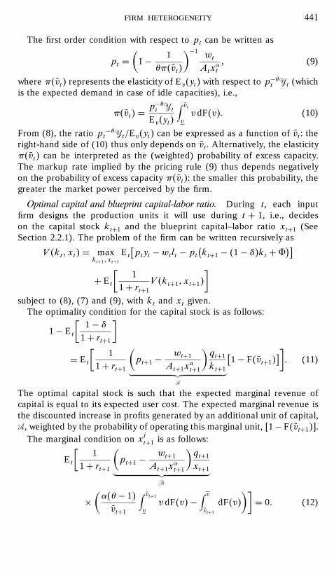
The first order condition with respect to pt can be written as

pt =(

1− 1θπ�vt�

)−1 wtAtx

αt

; (9)

where π�vt� represents the elasticity of Ev�yt� with respect to p−θt Yt (whichis the expected demand in case of idle capacities), i.e.,

π�vt� =p−θt Yt

Ev�yt�∫ vtvv dF�v�: (10)

From (8), the ratio pt−θYt/Ev�yt� can be expressed as a function of vt : theright-hand side of (10) thus only depends on vt . Alternatively, the elasticityπ�vt� can be interpreted as the (weighted) probability of excess capacity.The markup rate implied by the pricing rule (9) thus depends negativelyon the probability of excess capacity π�vt�: the smaller this probability, thegreater the market power perceived by the firm.

Optimal capital and blueprint capital-labor ratio. During t, each inputfirm designs the production units it will use during t + 1, i.e., decideson the capital stock kt+1 and the blueprint capital–labor ratio xt+1 (SeeSection 2.2.1). The problem of the firm can be written recursively as

V �kt; xt� = maxkt+1; xt+1

Et[ptyt −wtlt − pt

(kt+1 − �1− δ�kt +8

)]+ Et

[1

1+ rt+1V �kt+1; xt+1�

]subject to (8), (7) and (9), with kt and xt given.

The optimality condition for the capital stock is as follows:

1− Et

[1− δ

1+ rt+1

]= Et

[1

1+ rt+1

(pt+1 −

wt+1

At+1xαt+1

)qt+1

kt+1︸︷︷︸A

[1− F�vt+1�

]]: (11)

The optimal capital stock is such that the expected marginal revenue ofcapital is equal to its expected user cost. The expected marginal revenue isthe discounted increase in profits generated by an additional unit of capital,A, weighted by the probability of operating this marginal unit, �1−F�vt+1��.

The marginal condition on xjt+1 is as follows:

Et

[1

1+ rt+1

(pt+1 −

wt+1

At+1xαt+1

)qt+1

xt+1︸︷︷︸B

×(α�θ− 1�vt+1

∫ vt+1

vv dF�v� −

∫ vvt+1

dF�v�)]= 0: (12)


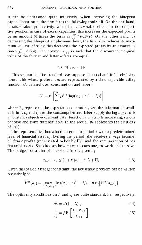
It can be understood quite intuitively. When increasing the blueprintcapital–labor ratio, the firm faces the following trade-off. On the one hand,it raises labor productivity, which has a favorable effect on its competi-tive position in case of excess capacities; this increases the expected profitsby an amount B times the term in

∫ vt+1v v dF�v�. On the other hand, by

decreasing the blueprint employment level, the firm also reduces its maxi-mum volume of sales; this decreases the expected profits by an amount Btimes

∫ vvt+1

dF�v�. The optimal xjt+1 is such that the discounted marginalvalue of the former and latter effects are equal.

2.3. Households

This section is quite standard. We suppose identical and infinitely livinghouseholds whose preferences are represented by a time separable utilityfunction Ut defined over consumption and labor:

Ut = Et

[∞∑s=tβs−t

(log�cs� + v�1− ls�

)]where Et represents the expectation operator given the information avail-able in t. cs and ls are the consumption and labor supply during s ≥ t. β isa constant subjective discount rate. Function v is strictly increasing, strictlyconcave and twice differentiable. In the sequel, vll represents the elasticityof v′�·�.

The representative household enters into period t with a predeterminedlevel of financial asset at . During the period, she receives a wage income,all firms’ profits (represented below by 5t), and the remuneration of herfinancial assets. She chooses how much to consume, to work and to save.The budget constraint of household in t is given by

at+1 + ct ≤ �1+ rt�at +wtlt +5t: (13)

Given this period t budget constraint, the household problem can be writtenrecursively as

V H�at� = maxct ; lt ; at+1

{log�ct� + v�1− lt� + βEt

[V H�at+1

]}The optimality conditions on lt and ct are quite standard, i.e., respectively,

wt = v′�1− lt�ct; (14)

1ct= βEt

[1+ rt+1

ct+1

]: (15)


2.4. General Equilibrium and Stationary State

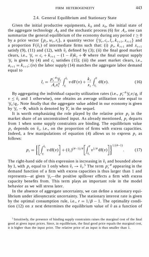
Given the initial productive equipments, k0 and x0, the initial state ofthe aggregate technology A0 and the stochastic process (6) for At , one cansummarize the general equilibrium of the economy during any period t ≥ 0by a price vector �pt;wt; rt�, a quantity vector �Yt ; ct; lt; kt+1; xt+1� anda proportion F�vt� of intermediate firms such that: (i) pt , kt+1 and xt+1satisfy (9), (11) and (12), with vt defined by (3); (ii) the final good marketclears, i.e., Yt = ct + kt+1 − �1 − δ�kt + 8 where the final output supplyYt is given by (4) and ct satisfies (15); (iii) the asset market clears, i.e.,at+1 = kt+1; (iv) the labor supply (14) matches the aggregate labor demandequal to

lt =p−θt Yt

Atxαt

∫ vtvv dF�v� + kt

xt

∫ vvt

df�v�: (16)

By aggregating the individual capacity utilization rates (i.e., p−θt Ytv/qt ifv ≤ vt and 1 otherwise), one obtains an average utilization rate equal toYt/qt . Note finally that the aggregate value added in our economy is givenby Yt −8, which is denoted by Yt in the sequel.

It is worth emphasizing the role played by the relative price pt in themarket share of an unconstrained input. As already mentioned, pt departsfrom 1 when some supply constraints are binding. The equilibrium valuept depends on vt , i.e., on the proportion of firms with excess capacities.Indeed, a few manipulations of equation (4) allows us to express pt asfollows:

pt ={[∫ vt

vv df�v�

]+ �vt��θ−1�/θ

[∫ vvt

v1/θ df�v�]}1/�θ−1�

: (17)

The right-hand side of this expression is increasing in vt and bounded aboveby 1, with pt equal to 1 only when vt → vt .5 The term p−θt appearing in thedemand function of a firm with excess capacities is thus larger than 1 andrepresents—at given Yt—the positive spillover effects a firm with excesscapacity benefits from. This term plays an important role in the modelbehavior as we will stress later.

In the absence of aggregate uncertainty, we can define a stationary equi-librium under idiosyncratic uncertainty. The stationary interest rate is givenby the optimal consumption rule, i.e., r = 1/β − 1. The optimality condi-tion (12) on x next determines the equilibrium value of v as a function of

5 Intuitively, the presence of binding supply constraints raises the marginal cost of the finalgood at given input prices. Since, in equilibrium, the final good price equals the marginal cost,it is higher than the input price. The relative price of an input is thus smaller than 1.


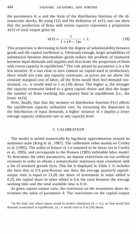
the parameters θ, α and the form of the distribution function of the id-iosyncratic shocks. By using (12) and the definition of π�v�, one can showthat the production of firms with excess capacity represents a proportionπ�v� of total output given by

π�v� = 11+ �θ− 1�α < 1: (18)

This proportion is decreasing in both the degree of substitutability betweengoods and the capital coefficient α. Obviously enough, larger possibilities ofsubstitution between intermediate goods reduce the problem of mismatchbetween input demands and supplies and thus lower the proportion of firmswith excess capacity in equilibrium.6 The role played by parameter α is a bitless intuitive. If α was close to zero (almost no capital used in production),there would not exist any capacity constraint; as prices are set above theconstant marginal cost of labor, all the firms would then feel demand con-strained, i.e., π would tend to 1 as (18) shows. The higher α, the strongerthe capacity constraint linked to a given capital choice and thus the largerthe number of firms reaching this capacity limit in equilibrium [i.e., thelower π�v�].

Note, finally, that that the variance of distribution function F�v� affectsthe equilibrium capacity utilization rate: by increasing the dispersion inthe distribution of input demands, a higher variance of v implies a loweraverage capacity utilization rate at any capacity level.

3. CALIBRATION

The model is solved numerically by log-linear approximation around itsstationary state (King et al., 1987). The calibration relies mainly on Cooleyet al. (1995). The utility of leisure v�·� is assumed to be linear (as in Cooleyet al., 1995), and corresponds to the Hansen (1985) indivisible labor model.To determine the other parameters, we impose restrictions on our artificialeconomy in order to obtain a nonstochastic stationary state consistent witha list of standard growth facts. This list is displayed in Table I. It includesthe facts that in US post-Korean war data, the average quarterly capital–output ratio is equal to 13.28, the share of investment in value added is0.25, the capital share in value added is 0.4, the ratio between the averageworking time and the total available time is 0.31.

At given capital–output ratio, the restriction on the investment share de-termines the value of parameter δ. The restrictions on the capital–output

6 In the limit case where inputs would be perfect substitutes (θ→∞), no firm would feeldemand constrained in equilibrium, i.e., π would tend to 0 as (18) shows.


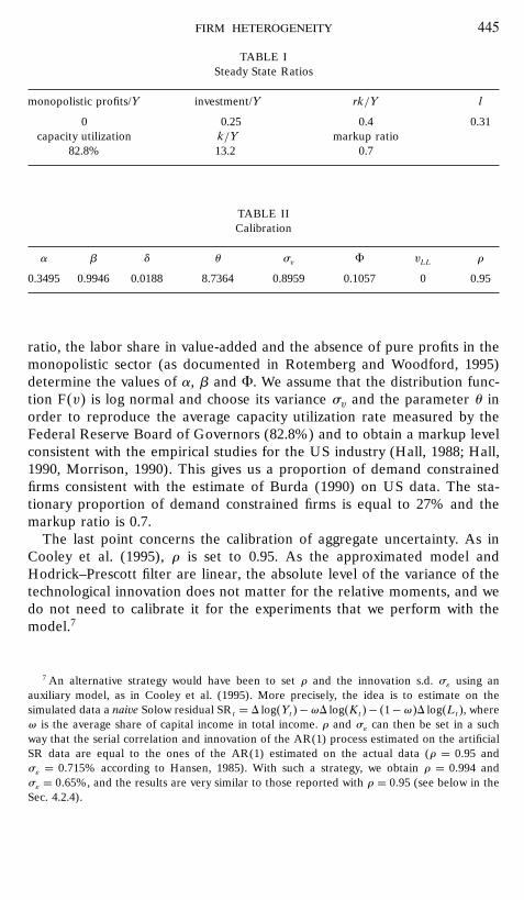
TABLE ISteady State Ratios

monopolistic profits/Y investment/Y rk/Y l

0 0.25 0.4 0.31capacity utilization k/Y markup ratio

82.8% 13.2 0.7

TABLE IICalibration

α β δ θ σv 8 vLL ρ

0.3495 0.9946 0.0188 8.7364 0.8959 0.1057 0 0.95

ratio, the labor share in value-added and the absence of pure profits in themonopolistic sector (as documented in Rotemberg and Woodford, 1995)determine the values of α, β and 8. We assume that the distribution func-tion F�v� is log normal and choose its variance σv and the parameter θ inorder to reproduce the average capacity utilization rate measured by theFederal Reserve Board of Governors (82.8%) and to obtain a markup levelconsistent with the empirical studies for the US industry (Hall, 1988; Hall,1990, Morrison, 1990). This gives us a proportion of demand constrainedfirms consistent with the estimate of Burda (1990) on US data. The sta-tionary proportion of demand constrained firms is equal to 27% and themarkup ratio is 0.7.

The last point concerns the calibration of aggregate uncertainty. As inCooley et al. (1995), ρ is set to 0.95. As the approximated model andHodrick–Prescott filter are linear, the absolute level of the variance of thetechnological innovation does not matter for the relative moments, and wedo not need to calibrate it for the experiments that we perform with themodel.7

7 An alternative strategy would have been to set ρ and the innovation s.d. σε using anauxiliary model, as in Cooley et al. (1995). More precisely, the idea is to estimate on thesimulated data a naive Solow residual SRt = 1 log�Yt�−ω1 log�Kt�− �1−ω�1 log�Lt�, whereω is the average share of capital income in total income. ρ and σε can then be set in a suchway that the serial correlation and innovation of the AR(1) process estimated on the artificialSR data are equal to the ones of the AR(1) estimated on the actual data (ρ = 0:95 andσε = 0:715% according to Hansen, 1985). With such a strategy, we obtain ρ = 0:994 andσε = 0:65%, and the results are very similar to those reported with ρ = 0:95 (see below in theSec. 4.2.4).


4. RESULTS

4.1. Impulse Responses to an Aggregate Technological Shock

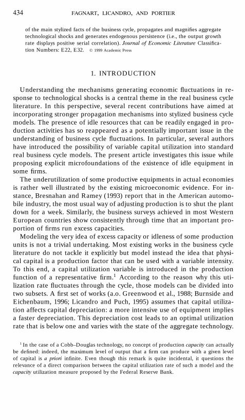
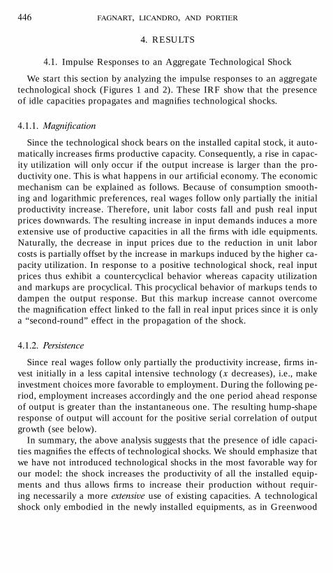
We start this section by analyzing the impulse responses to an aggregatetechnological shock (Figures 1 and 2). These IRF show that the presenceof idle capacities propagates and magnifies technological shocks.

4.1.1. Magnification

Since the technological shock bears on the installed capital stock, it auto-matically increases firms productive capacity. Consequently, a rise in capac-ity utilization will only occur if the output increase is larger than the pro-ductivity one. This is what happens in our artificial economy. The economicmechanism can be explained as follows. Because of consumption smooth-ing and logarithmic preferences, real wages follow only partially the initialproductivity increase. Therefore, unit labor costs fall and push real inputprices downwards. The resulting increase in input demands induces a moreextensive use of productive capacities in all the firms with idle equipments.Naturally, the decrease in input prices due to the reduction in unit laborcosts is partially offset by the increase in markups induced by the higher ca-pacity utilization. In response to a positive technological shock, real inputprices thus exhibit a countercyclical behavior whereas capacity utilizationand markups are procyclical. This procyclical behavior of markups tends todampen the output response. But this markup increase cannot overcomethe magnification effect linked to the fall in real input prices since it is onlya “second-round” effect in the propagation of the shock.

4.1.2. Persistence

Since real wages follow only partially the productivity increase, firms in-vest initially in a less capital intensive technology (x decreases), i.e., makeinvestment choices more favorable to employment. During the following pe-riod, employment increases accordingly and the one period ahead responseof output is greater than the instantaneous one. The resulting hump-shaperesponse of output will account for the positive serial correlation of outputgrowth (see below).

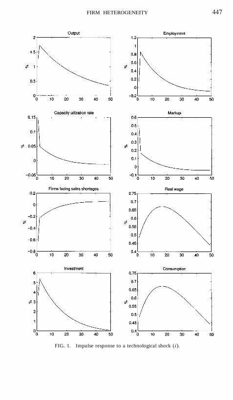
In summary, the above analysis suggests that the presence of idle capaci-ties magnifies the effects of technological shocks. We should emphasize thatwe have not introduced technological shocks in the most favorable way forour model: the shock increases the productivity of all the installed equip-ments and thus allows firms to increase their production without requir-ing necessarily a more extensive use of existing capacities. A technologicalshock only embodied in the newly installed equipments, as in Greenwood


FIG. 1. Impulse response to a technological shock �i�.


FIGURE 2

et al. (1988), would have implied more variation in the capacity utilizationmargin.

4.2. Simulation Results

All the simulated series have been detrended by using the Hodrick–Prescott filter. The results are obtained from 100 simulations of 150 pointseach.

4.2.1. The Artificial Business Cycle

The artificial business cycle displayed by the model is given in Table III.The “data” columns correspond to quarterly US time series from 1954:1 to1991:3. Output is gross national product, consumption corresponds to pur-chases of nondurable and services, and investment (I in Table III) is fixedinvestment. All these variables are measured in 1982 dollars. Hours rep-resent total weekly hours in all industries based on the current populationsurvey.

The relative variations of investment and consumption are well repro-duced. Hours are slightly more variable than productivity. As in the USbusiness cycle, the variability of the labor share is about one-third of the


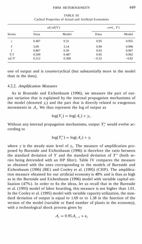
TABLE IIICyclical Properties of Actual and Artificial Economies

sd/sd�Y � cor�·; Y �Series Data Model Data Model

c 0.497 0.31 0.95 0.955

I 3.09 3.14 0.99 0.996l 0.867 0.50 0.93 0.907Y/l 0.509 0.487 0.95 0.902wl/Y 0.312 0.308 −0.32 −0.82

one of output and is countercyclical (but substantially more in the modelthan in the data).

4.2.2. Amplification Measures

As in Brunside and Eichenbaum (1996), we measure the part of out-put variation that is explained by the internal propagation mechanisms ofthe model (denoted yt) and the part that is directly related to exogenousmovements in At . We thus represent the log of output as

log�Yt� = log�At� + yt :Without any internal propagation mechanisms, output Y ∗t would evolve ac-cording to

log�Y ∗t � = log�At� + y;where y is the steady state level of yt . The measure of amplification pro-posed by Burnside and Eichenbaum (1996) is therefore the ratio betweenthe standard deviation of Y and the standard deviation of Y ∗ (both se-ries being detrended with an HP filter). Table IV compares the measureso obtained with the ones corresponding to the models of Burnside andEichenbaum (1996) (BE) and Cooley et al. (1995) (CHP). The amplifica-tion measure obtained for our artificial economy is 48% and is thus as highas in the Burnside and Eichenbaum (1996) model with variable capital uti-lization (47%). In order to fix the ideas, let us recall that in the Burnsideet al. (1993) model of labor hoarding, this measure is not higher than 1.01.In the Cooley et al. (1995) model with variable capacity utilization, the stan-dard deviation of output is equal to 1.69 or to 1.38 in the function of theversion of the model (variable or fixed number of plants in the economy),with a technological shock process given by

At = 0:95At−1 + εt


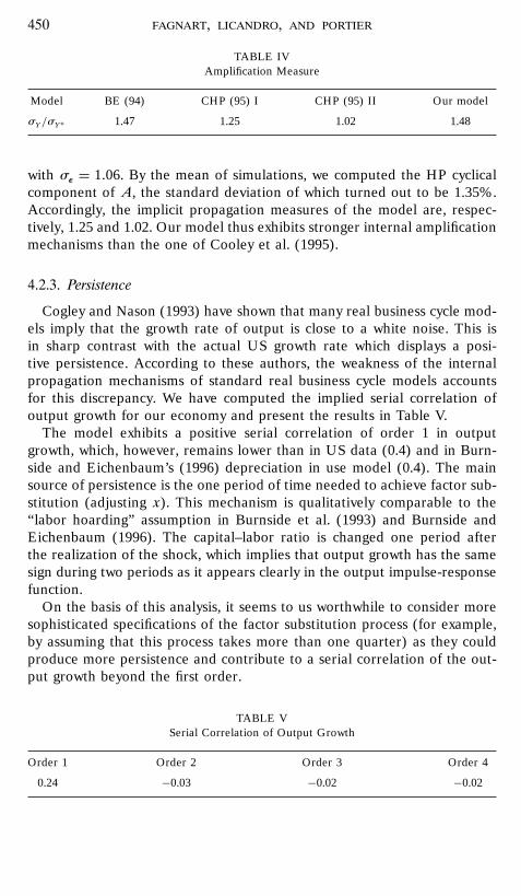
TABLE IVAmplification Measure

Model BE (94) CHP (95) I CHP (95) II Our model

σY/σY∗ 1.47 1.25 1.02 1.48

with σε = 1:06. By the mean of simulations, we computed the HP cyclicalcomponent of A, the standard deviation of which turned out to be 1.35%.Accordingly, the implicit propagation measures of the model are, respec-tively, 1.25 and 1.02. Our model thus exhibits stronger internal amplificationmechanisms than the one of Cooley et al. (1995).

4.2.3. Persistence

Cogley and Nason (1993) have shown that many real business cycle mod-els imply that the growth rate of output is close to a white noise. This isin sharp contrast with the actual US growth rate which displays a posi-tive persistence. According to these authors, the weakness of the internalpropagation mechanisms of standard real business cycle models accountsfor this discrepancy. We have computed the implied serial correlation ofoutput growth for our economy and present the results in Table V.

The model exhibits a positive serial correlation of order 1 in outputgrowth, which, however, remains lower than in US data (0.4) and in Burn-side and Eichenbaum’s (1996) depreciation in use model (0.4). The mainsource of persistence is the one period of time needed to achieve factor sub-stitution (adjusting x). This mechanism is qualitatively comparable to the“labor hoarding” assumption in Burnside et al. (1993) and Burnside andEichenbaum (1996). The capital–labor ratio is changed one period afterthe realization of the shock, which implies that output growth has the samesign during two periods as it appears clearly in the output impulse-responsefunction.

On the basis of this analysis, it seems to us worthwhile to consider moresophisticated specifications of the factor substitution process (for example,by assuming that this process takes more than one quarter) as they couldproduce more persistence and contribute to a serial correlation of the out-put growth beyond the first order.

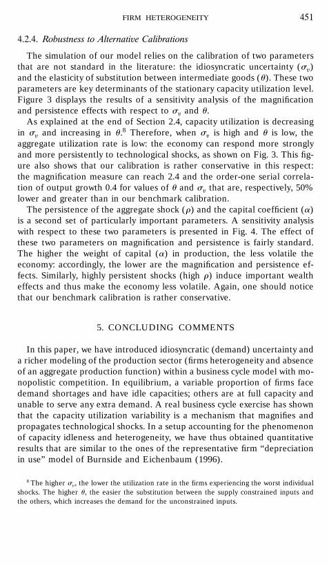
TABLE VSerial Correlation of Output Growth

Order 1 Order 2 Order 3 Order 4

0.24 −0.03 −0.02 −0.02


4.2.4. Robustness to Alternative Calibrations

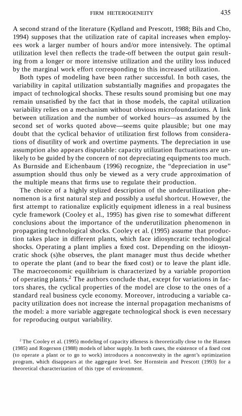
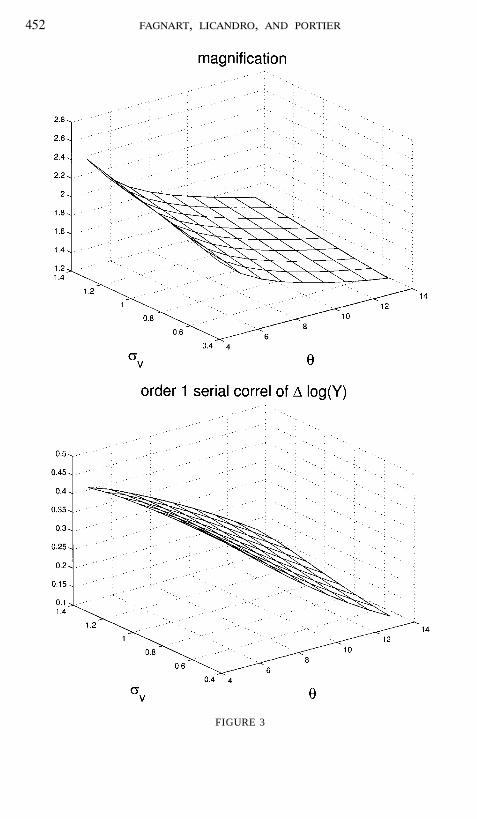
The simulation of our model relies on the calibration of two parametersthat are not standard in the literature: the idiosyncratic uncertainty (σv)and the elasticity of substitution between intermediate goods (θ). These twoparameters are key determinants of the stationary capacity utilization level.Figure 3 displays the results of a sensitivity analysis of the magnificationand persistence effects with respect to σv and θ.

As explained at the end of Section 2.4, capacity utilization is decreasingin σv and increasing in θ.8 Therefore, when σv is high and θ is low, theaggregate utilization rate is low: the economy can respond more stronglyand more persistently to technological shocks, as shown on Fig. 3. This fig-ure also shows that our calibration is rather conservative in this respect:the magnification measure can reach 2.4 and the order-one serial correla-tion of output growth 0.4 for values of θ and σv that are, respectively, 50%lower and greater than in our benchmark calibration.

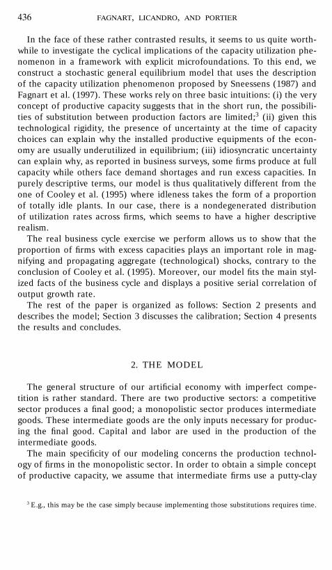
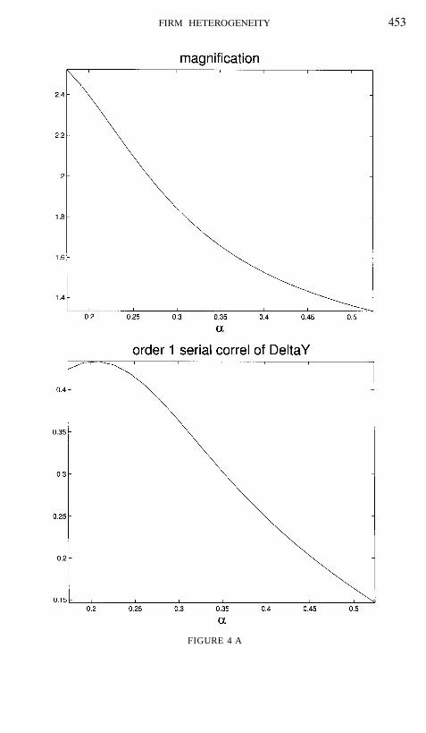
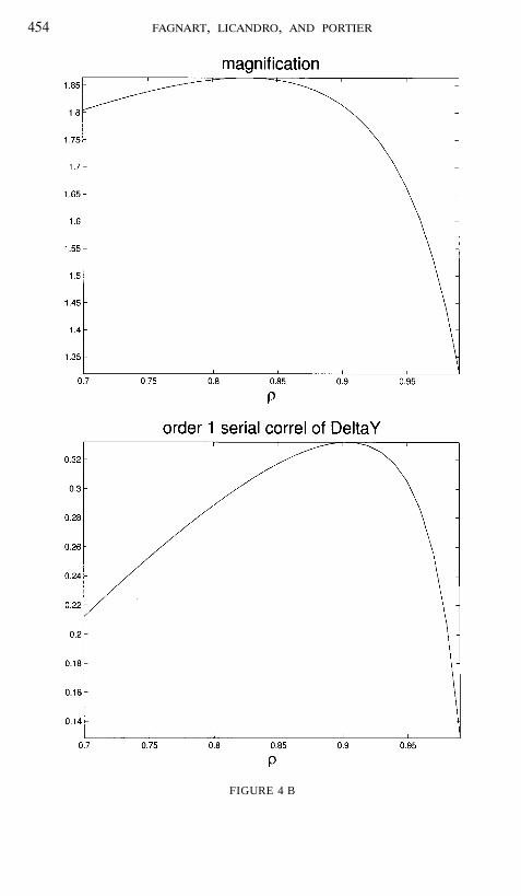
The persistence of the aggregate shock (ρ) and the capital coefficient (α)is a second set of particularly important parameters. A sensitivity analysiswith respect to these two parameters is presented in Fig. 4. The effect ofthese two parameters on magnification and persistence is fairly standard.The higher the weight of capital (α) in production, the less volatile theeconomy: accordingly, the lower are the magnification and persistence ef-fects. Similarly, highly persistent shocks (high ρ) induce important wealtheffects and thus make the economy less volatile. Again, one should noticethat our benchmark calibration is rather conservative.

5. CONCLUDING COMMENTS

In this paper, we have introduced idiosyncratic (demand) uncertainty anda richer modeling of the production sector (firms heterogeneity and absenceof an aggregate production function) within a business cycle model with mo-nopolistic competition. In equilibrium, a variable proportion of firms facedemand shortages and have idle capacities; others are at full capacity andunable to serve any extra demand. A real business cycle exercise has shownthat the capacity utilization variability is a mechanism that magnifies andpropagates technological shocks. In a setup accounting for the phenomenonof capacity idleness and heterogeneity, we have thus obtained quantitativeresults that are similar to the ones of the representative firm “depreciationin use” model of Burnside and Eichenbaum (1996).

8 The higher σv, the lower the utilization rate in the firms experiencing the worst individualshocks. The higher θ, the easier the substitution between the supply constrained inputs andthe others, which increases the demand for the unconstrained inputs.


FIGURE 3


FIGURE 4 A


FIGURE 4 B


REFERENCES

Bils, M., and Cho, J-O. (1994). “Cyclical factor utilization,” Journal of Monetary Economics33, 319–354.

Bresnahan, T., and Ramey, V. (1993). “Segment shifts and capacity utilization in the U.S.automobile industry,” American Economic Review 83, 213–218.

Burda, M. (1990). “Is Mismatch Really the Problem? Some Estimates of the Chelwood GateII model with U.S. Data,” in Europe’s Unemployment Problem (J. Dreze and C. Bean, Eds.),pp. 451–79. Cambridge, MA: MIT Press.

Burnside, C., and Eichenbaum, M. (1996). “Factor hoarding and the propagation of businesscycle shocks,” American Economic Review 86, 1157–1174.

Burnside, C., Eichenbaum, M., and Rebelo, S. (1993). “Labor hoarding and the businesscycle,” Journal of Political Economy 101(2), 104–121.

Clower, R. (1967). “A reconsideration of the microfoundations of money,” Western EconomicJournal 6(4), 1–9.

Cogley, J., and Nason, T. (1993). “Do Real Business Cycles Models Pass the Nelson–PlosserTest?” Working paper, University of British Columbia.

Cooley, T., Hansen, G., and Prescott, E. (1995). “Equilibrium business cycle with idle resourcesand variable capacity utilization,” Economic Theory 6, 35–49.

Fagnart, J. F., Licandro, O., and Sneessens, H. (1997). “Capacity Utilization Dynamics andMarket Power,” Journal of Economic Dynamics and Control 22, 123–140.

Greenwood, J., Hercowitz, Z., and Huffman, G. (1998). “Investment, capacity utilisation, andthe real business cycle,” American Economic Review 78, 402–417.

Hall, R. (1988). “The relation between price and marginal cost in U.S. industry,” Journal ofPolitical Economy 96, 921–948.

Hall, R. (1990). “Invariance Properties of Solow’s Productivity Residual,” in Growth, Pro-ductivity and Unemployment, Essays to Celebrate Bob Solow’s Birthday (P. Diamond, Ed.).Cambridge, MA: MIT Press.

Hansen, G. (1985). “Indivisible labor and the business cycles,” Journal of Monetary Economics16(3), 309–327.

Hornstein, A., and Prescott, E. (1993). “The firm and the plant in general equilibrium the-ory,” in General Equilibrium, Growth and Trade II (R. Becker, M. Boldrin, R. Jones, andW. Thomson, Eds.). San Diego: Academic.

King, R., Plosser, C., and Rebelo, S. (1987). “Production Growth and Business Cycles: Tech-nical Appendix,” Working paper, University of Rochester (revised May 1990).

Kydland, F., and Prescott, E. (1988). “The workweek of capital and its cyclical implications,”Journal of Monetary Economics 21(2/3), 343–360.

Licandro, O., and Puch, L. (1995). “Capacity Utilization, Maintenance Costs and the Busi-ness Cycle,” Working paper 95-34, Universidad Carlos III de Madrid (forthcoming Annalesd’Economie et de Statistique).

Morrison, C. (1990). “Market Power, Economic Profitability and Productivity Growth Mea-surement: an Integrated Structural Approach,” Working paper 3355, National Bureau ofEconomic Research.

Rogerson, R. (1988). “Indivisible labor, lotteries and equilibrium,” Journal of Monetary Eco-nomics 21(1), 3–16.

Rotemberg, J., and Woodford, M. (1995). “Dynamic general equilibrium models with imper-fectly competitive product markets,” in Frontiers of Business Cycle Research (T. Cooley, Ed.).Princeton, NJ: Princeton University Press.

Sneessens, H. (1987). “Investment and the inflation-unemployment tradeoff in a macroeco-nomic rationing model with monopolistic competition,” European Economic Review 31, 781–815.

firm heterogeneity, capacity utilization, and the … fagnart, licandro, and portier of the main...

Documents