Firm-Specificity of Asset, Managerial Capability,

and Labor Market Competition

Hodaka Morita∗ Cheng-Tao Tang†

July 2018

∗School of Economics, University of New South Wales. Email: hodakamorita@gmail.com†GSIR, International University of Japan. Email: chengtao.tang@gmail.com

Abstract

We develop a model that captures the link between specificity of a firm’s asset and capa-

bility of the firm’s top management, two important sources of profitability. It contributes

to strands of economics and management literature by proposing a logic through which

firm-specificity and heterogeneity are determined endogenously through labor market

competition. Higher importance of managerial capability raises labor mobility, which

reduces firm-specificity of asset and human capital, and firm size, whereas higher im-

portance of asset specificity yields opposite effects. Our findings yield novel empirical

implications and predictions, given that the importance of managerial capability differs

across industries, countries and time.Â

1 Introduction

Firms let their employees operate their assets to produce and sell goods and services.

Specificity of a firm’s asset and capability of its top management are two important

sources of the firm’s profitability. In this paper, we develop a new theoretical model that

captures the link between specificity of a firm’s asset and capability of the firm’s top

management, where the degree of firm-specificity is endogenously determined through

firms’ competition in the labor market.

In the resource-based view of the firm (Wernerfelt, 1984; Barney, 1991), firm-specificity

of the asset, often referred to as heterogeneity of firm resources (physical capital, human

capital, and organizational capital resources), has been identified as a critical source of

sustained competitive advantage. The point here is that heterogeneity of firm resources

enables a firm to conceive and implement a value-creating strategy that is unique and

unable to be imitated by other firms, leading the firm to establish a sustained competi-

tive advantage (Barney, 1991). Among the three broad categories of firm resources just

mentioned, in this paper we focus on physical capital resources, human capital resources,

and the interaction between the two.

In transaction cost economics (Williamson, 1979; 1985), firm-specificity of an asset,

referred to as asset specificity, also serves as a key concept in the analysis of governance

structure. If a seller tailors the nature of its physical capital specifically to its trans-

actions with a buyer, the seller can increase efficiency of its production for the buyer

(Williamson, 1979; Riordan and Williamson, 1985). Furthermore, there is an impor-

tant link between relation specificity of physical capital and human capital, because,

if employees operate firm-specific physical capital, their training and learning-by-doing

to operate the physical capital also become firm-specific (Williamson, 1979). In our

theoretical model, we incorporate this link, which is a key element for the endogenous

determination of firm-specificity of asset and human capital in the presence of labor

market competition.

The capability of a firm’s top management is a critical determinant of the firm’s prof-

itability, because it is the top management that sets the strategy for the firm, determines

its organizational structure, and establishes systems and processes for implementing the

strategy (Porter and Nohria, 2010). It has been widely recognized that the capabilities

1

of top managements differ across firms. Several papers have explored theoretical models

in which an individual with higher managerial talent assumes a top position of a larger

firm (see Lucas, 1978; Rosen, 1982; Gabaix and Landier, 2008; Terviö, 2008).1

In our model, a firm that has realized a high managerial capability hires some workers

from a firm that has realized a low managerial capability. The labor mobility generated

by ex ante uncertainty of firms’ managerial capabilities plays a key role in the endoge-

nous determination of firm-specificity of asset and human capital. It has been widely

recognized that capabilities of top managements are mostly innate, uncertain, and ex

ante unknown.2 Given the uncertainty, Pan, Wang and Weisbach (2015) empirically

study the process through which the market learns about the CEO’s ability, and Denis,

Denis and Walker’s (2015) empirical study concludes that the need for assessment of the

CEO’s ability is an important element of the structure of newly formed boards. Closely

related to the uncertainty of top managements’ capabilities, several papers have studied

firm-dynamics models in which the efficiency of firms in an industry is different across

firms, and no firm knows its own true efficiency ex ante (Jovanovic, 1982; Lippman and

Rumelt, 1982; Hopenhayn, 1992).

The importance of top management’s capability (hereafter referred to as managerial

capability) differs across an industry’s life cycle, countries, and time. For instance, as an

industry evolves from infancy stage, firms typically undergo revolutionary technological

changes. Thus, a business’s success depends on the quality of its strategic decision mak-

ing because firms during this stage are surrounded by a high level of uncertainty about

the needs of customers, the products and services that will prove to be the most desired,

and the best configuration of activities and technologies to deliver them. Whereas in the

mature phase of an industry, institutional structures become clear and the opportunity

for radical innovation is few. These arguments suggest that the importance of managerial

capability is higher during the early phase of an industry’s life cycle with revolutionary

technological changes and higher level of uncertainty, while the importance tends to be

lower in the mature phase of an industry with less technological advancement and lower1See also Oi (1983) for a related analysis.2As Goleman (1998) puts it, “Every business person knows a story about a highly intelligent, highly

skilled executive who was promoted into a leadership position only to fail at the job. And they also knowa story about someone with solid—but not extraordinary—intellectual abilities and technical skills whowas promoted into a similar position and then soared. See also Aaker (2011), who points out that agifted CEO needs two qualities, executive talent and strategic judgement, which come with birth, andnot training in his view.

2

level of uncertainty.

How do differences in the importance of managerial capability affect firm-specificity

of assets, the nature of human capital acquisition within firms, firm size, and labor mo-

bility? Our two-period duopoly model of labor market competition provides an answer

to this question. We find that, as the importance of managerial capability increases,

firms make their asset less firm-specific, a smaller number of workers are hired (implying

smaller average firm size), and labor mobility increases. Also, lower firm-specificity of

asset leads to lower firm-specificity of skills acquired by workers.

The logic behind our result is as follows. In period 1, each firm hires a certain number

of workers and determines the degree of firm-specificity of its asset (physical capital)

without knowing its own managerial capabilities. As the importance of managerial

capability increases, each firm anticipates that a larger number of workers switch their

employers in period 2. This is because the higher importance of managerial capability

makes firms’ productivity more sensitive to their managerial capabilities, implying that

period 2 productivity between a high-capability and a low-capability firm becomes larger.

Anticipation of the higher labor turnover rate decreases a firm’s incentive to invest in

raising firm-specificity of its asset, because higher firm-specificity of the asset increases

its worker’s period 2 output only if the worker is already familiarized with firm-specific

nature of the firm’s asset through period 1 employment in the same firm. Lower asset

specificity increases transferability of the firm’s employees skills to the other firm and

hence reduces firm-specificity of their human capital. The link between asset specificity

and firm-specificity of human capital, not emphasized in the existing literature, is a

driving force of our key results.

A higher labor turnover rate leads to lower firm-specificity of the asset, which, in

turn, reduces each firm’s incentive to hire workers in period 1, through two channels.

First, lower firm-specificity reduces period-2 output of a retained worker. Second, lower

firm-specificity increases the fraction of workers who switch employers in period 2. These

two effects together reduce the expected period-2 productivity of each period-1 worker,

implying that the number of workers employed by each firm in period 1 decreases as the

importance of managerial capability increases.

Our theoretical framework yields empirical implications and predictions from a pre-

viously unexplored perspective. First, it enriches a prediction of transaction cost eco-

3

nomics (TCE) on the relationship between uncertainty and governance structure by

indicating that uncertainty has an indirect effect on vertical integration transmitting

through asset specificity. In TCE, the three critical dimensions for characterizing trans-

actions are uncertainty, the frequency with which transactions recur, and the degree to

which transaction-specific investments are incurred (that is, the degree of asset speci-

ficity) (Williamson, 1979; 1985). A standard prediction of TCE is that, in line with asset

specificity and frequent transactions, higher uncertainty makes vertical integration more

likely. This TCE prediction holds true in our framework only if uncertainty’s positive

direct effect outweighs its negative indirect effect; while the opposite relationship, not

compatible with TCE prediction, is still suited in ours. Existing empirical evidence on

this TCE prediction, in fact, are rather mixed, suggesting that channels through which

uncertainty affects the likelihood of vertical integration can be richer than the standard

one. Our analysis contributes to the TCE literature by pointing out a possible new

channel and its implication in estimation. See Section 5.1 for details.

Furthermore, given that the importance of managerial capability can differ as an

industry goes through stages of its life cycle, our model predicts that labor mobility is

higher, specificity of asset and human capital is lower, and average firm size is smaller

in the early or growing phases of an industry’s life cycle that features rapid change

of markets and disruptive technologies. Also, as the economy makes a transition from

industrial capitalism to post-industrial capitalism, modern economies are becoming in-

creasingly knowledge-intensive which renders the disadvantage to the firms that heavily

rely on physical assets. This aspect allows us to apply the model results in explaining

the observed difference in the labor mobility, specificity of asset and human capital, and

firm size across countries and time (see Section 5.2 and 5.3 for more discussions).

2 Relationships with literature

As mentioned in the previous section, our theoretical analysis makes a contribution to

TCE by proposing a new prediction on the relationship between uncertainty and gover-

nance structure. In this section, we discuss our contributions to the resource-based view

(RBV) of the firm and the human capital theory. In the RBV literature, several authors

have pointed out the importance of developing a theory in which firm heterogeneity,

4

the central concept of the RBV, is determined endogenously rather than assumed ex-

gonenouly (see Mahoney and Pandian, 1992; Helfat and Peteraf, 2003; Hoopes, Madsen

and Walker, 2003). Mahoney and Pandian (1992), for example, point out, “A major ad-

vancement in the strategy field is the development of models where firm heterogeneity

is an endogenous creation of economic actors."

As mentioned earlier, several papers have previously explored models in which an

individual with higher managerial talent assumes a top position of a larger firm (Lucas,

1978; Rosen, 1982; Gabaix and Landier, 2008; Terviö, 2008). These papers can be viewed

as contributions to the RBV literature because they analyse the process in which the

distribution of managerial capabilities endogenously determines the size distribution of

firms, where the difference in firm size is an important element of firm heterogeneity.

Our contribution to the RBV literature is complementary to these earlier contribu-

tions. As in these models, the distribution of managerial capabilities (which is assumed

to be binary in our model for simplicity) is the driving force of firm heterogeneity in our

model. However, elements of firm heterogeneity determined endogenously and the logic

behind the determination in our model are fundamentally different from those in the ear-

lier models. That is, in our model, firm heterogeneities of physical capital and human

capital are the key elements that are endogenously determined, and these heterogeneities

in turn lead to heterogeneity in firm size as well.

Labor mobility generated by ex ante uncertainty of managerial capabilities and the

link between firm-specificities of asset and human capital are the driving forces of firm

heterogeneities of physical capital and human capital, which in turn determine the aver-

age firm size in our model. Consistent with the earlier models, our model also captures

the idea that a firm with higher managerial capability ends up with a larger firm size

in the sense that some workers move from a low capability firm to a high capability

firm in our model. See Murphy and Zabojnik (2004) for a related model, which an-

alyze interconnections among the CEO’s managerial capability, firm-specificity of the

capability, and the optimal firm size. Murphy and Zabojnik (2004) show that, as the

relative importance of firm-specific managerial capability decreases, the importance of

the match between managerial capability and firm size increases, implying that filling

CEO positions with outside hires rather than internal candidates become more likely.

Firm-specificity of managerial capability is an exogenous parameter in their model.

5

Parallel to our contribution to the RBV literature, we contribute to the human

capital theory literature by analysing the process in which firm-specificity of human

capital is endogenously determined. Since the seminal contribution by Becker (1962),

the distinction between general and firm-specific human capital has played an important

role in the literature. Firm-specific human capital raises the productivity of the worker at

his current firm but not elsewhere, whereas general human capital increases the worker’s

productivity at his current firm and at other firms.

To the best of our knowledge, firm-specificity of human capital is exogenously as-

sumed in most exisiting models of human capital, but there are several recent exceptions

including Morita (2001) and Lazear (2009). Our contribution to the literature is comple-

mentary to these earlier contributions, but the nature and the logic behind determination

of firm-specificity in our model are fundamentally different from those in their models.

Morita (2001) proposes a model of labor market competition in which multiplicity

of equilibria provides an explanation for the U.S.-Japanese differences in employment

practices and the nature of technological improvement. The model assumes that, if

a firm conducts continuous process improvement, the firm’s technology is improved

but a degree of firm-specificity is introduced. The link between continuous process

improvement and the firm-specificity of training, along with labor mobility generated

by stochastic worker-firm match qualities, lead to strategic complementarity, which in

turn causes multiplicity of equilibria. In the Japanese equilibrium, each firm conducts

continuous process improvement because other firms do so, and as a consequence training

provided by such a firm becomes less effective (more firm-specific) in other firms. This

lowers the turnover rate, which, in turn, increases firms’ incentives to train employees.

In the U.S. equilibrium, training is general, which raises the turnover rate and decreases

incentives to train.

Our model is related to Morita’s (2001) model in the sense that the link between firm-

specificity of asset and firm-specificity of human capital, a driving force of our results,

is similar to the link between continuous process improvement and firm-specificity of

training. The key logic and insight, however, are different. In our model, it is ex ante

uncertainty of managerial capabilities, not worker-firm match qualities, that generates

labor turnover. As the importance of managerial capability increases, firms anticipate a

higher labor turnover rate, and this reduces asset specificity, firm-specificity of human

6

capital, and firm size, in equilibrium. Comparative statics analyses with respect to the

importance of managerial capability yield key results and implications in our model,

whereas an explanation for cross-country differences based on multiplicity of equilibria,

which does not arise in our model, is the key insight of Morita’s (2001) model.

Notice that, regarding uncertainty, our focus is on uncertainty of managerial capa-

bility, whereas uncertainty in labour productivity is another important issue. Bai and

Wang (2003) analyze a fixed wage contract model to study the effects of uncertainty in

labor productivity on investment in firm-specific human capital (SHC), wage and the

probability of separation. They find that wage and SHC are always positively corre-

lated, but SHC investment and the probability of separation do not have a monotonic

relationship. Human capital is assumed to be firm-specific in Bai and Wang’s (2003)

model, and hence endogenous determination of firm-specificity of human capital is not

an issue there.

Lazear (2009) and Gathmann and Schönberg (2010) propose a new theory of hu-

man capital in which all skills are general but firms use them with different weights

attached. The difference in skill-weights determines firm-specificity (or transferability)

of the worker’s skill set in their models. In Lazear’s (2009) approach, workers are ex-

ogenously assigned to a firm and then choose how much to invest in each skill. In

Gathmann and Schönberg’s (2010) approach, each worker is endowed with a produc-

tivity in each skill and then chooses an occupation, where different occupations have

different skill-weights. An important difference between these models and our model is

that the difference in skill-weights is exogenously assumed in the former, whereas the

degree of firm-specificity is endogenously determined in the latter.

3 The model

Consider an industry with two ex ante identical firms in a two-period setting. Only one

homogenous good is produced in this industry and the price is normalized to one. Labor

is the only input, and a firm’s output is a summation of its employees’ outputs. There

exists a large number of individuals, where each individual is of measure zero. In each

period, labor supply is perfectly inelastic and fixed at one unit for each individual. To

keep the analysis simple, firms and individuals do not discount the future, and they are

7

risk-neutral.

At the beginning of period 1, each individual has the same general human capital

and looks identical to the firms. Each individual can apply to a firm for employment.

Each firm i simultaneously makes a first-period wage offer wi,1 to hire desired number

of individuals from its applicants. Let ni denote the number of firm i’s first-period

employees. Individuals not employed by a firm become self-employed and remain so

until the end of period 2, earning ω > 0 per period.

Each firm’s production efficiency is determined by its managerial capability and the

level of its asset specificity, where managerial capability is interpreted as representing

the ability of a firm’s top management to develop an effective strategy and a unique

competitive position. The realization of firm i’s managerial capability ai is given by

ai = k + xi, where xi reflects a mean-preserving shock according to a symmetric binary

distribution with Pr(xi = x) = Pr(xi = −x) = 12 and k(≥ 0) is the mean of the

managerial capability. This specification is consistent with the widely held view that

the ability of a firm’s top management is mostly innate, and difficult to observe or assess

ex ante. Each firm i’s managerial capability ai becomes common knowledge at the end

of the period 1 operation.

Higher managerial capability ai increases firm i’s production efficiency by increasing

its worker’s output. Notice that the difference of managerial capabilities between a high-

capability and a low-capability firm, 2x, represents the sensitivity of firms’ production

efficiency to their managerial capabilities. Hence we interpret that the parameter x

represents the importance of managerial capability, which increases as firms’ productivity

becomes more sensitive to the difference of their managerial capabilities. In contrast,

the parameter k does not capture the importance of managerial capability because it

remains constant whether the firm’s managerial capability is high or low.

Also at the beginning of period 1, each firm i can invest zi ≥ 0 in its level of asset

specificity at a cost of c(zi) ≥ 0, where c(·) is a convex function. The asset specificity

refers to the extent to which a firm tailors its non-human asset for its particular use. To

obtain closed-form solutions in the analysis, let c(z) = 12θz

2 and θ > 0.

Each firm chooses its level of asset specificity at the same time as making its first-

period wage offer to individuals, and commits to the investment level. Any worker

employed by a firm in period 1 acquires a certain level of industry specific skill, which

8

increases the worker’s second-period productivity by d (a positive constant). At the

same time, a worker gets familiarized with the specificity of his first-period employer i’s

asset through learning-by-doing in period 1. If the worker is retained by the same firm

in period 2, his familiarity with asset specificity increases his second-period productivity

by f(zi), where f(0) = 0 and f ′(zi) > 0 for all zi ≥ 0. That is, a higher level of asset

specificity increases a worker’s second-period productivity if the worker has already

familiarized with it. Taken together, if a worker stays with his period 1 employer i

in period 2, his second-period production efficiency is d + f(zi), whereas, if a worker

switches his employers between periods 1 and 2, his second-period production efficiency

is d. Without loss of generality, we assume that d = 1. And to obtain closed-form

solutions, let f(zi) = szi where s > 0. Here s captures the importance of a firm’s asset

specificity on its retained workers.

To produce the good, each worker also requires employer supervision. Assume that

firm i’s per worker supervision cost is bni in each period, where b > 0. That is, as

the number of workers increases, each worker’s net output declines because each worker

receives less supervision from the employer.3 Each firm i’s period 1 profit is

niai − bn2i −1

2θz2i −Wi,1,

where Wi,1 denotes firm i’s first-period total wage bill.

At the beginning of period 2, each firm i can make its second-period wage offer wij

(i 6= j) to poach firm j’s employees, and can also make offer wii to retain its period 1

employees. Each worker can apply for one firm. Each firm can hire a desired number

of workers from its applicants. If a worker applied for a firm and not hired, then the

worker must take an outside option. Note that, when a firm makes wage offers, it knows

its realization of managerial capability. Hence, the wage offer can be different across

retained workers and new hires. Let mi(> −ni) denote either the number of firm i’s

newly hired workers in the second period if mi ≥ 0, or the number of dismissed workers3See Zábojník and Bernhardt (2001) and DeVaro and Morita (2013) for a similar specification.

9

if mi < 0. Each firm i’s period 2 profit is

ni(ai + 1 + szi) +mi(ai + 1)− b (ni +mi)

2 −Wi,2 if mi ≥ 0

(ni +mi) (ai + 1 + szi)− b (ni +mi)2 −Wi,2 if mi < 0

,

whereWi,2 denotes firm i ’s second-period total wage bill. Firm i expands in its firm size

if the net change in the number of workers in period 2 is positive; firm i contracts in its

firm size if the net change in the number of workers is negative. A firm stays unchanged

in its size only if it does not expand nor contract.

The timing of the game is as follows.

Period 1

[Stage 1] Each individual can apply to a firm or become self-employment. Each firm i

simultaneously makes first-period wage offers wi,1 to hire desired number of individuals

from its applicants, where i = 1, 2. At the same time, each firm chooses its level of

asset specificity zi by incurring a cost. Each individual can apply to a firm or become

self-employed. Individuals choose to work for a firm when indifferent between accepting

wage offers and self-employment. Self-employed workers remain so for both periods,

earning a wage ω each period.

[Stage 2] Each firm i that employed ni workers at Stage 1 produces niai units of the

good. At the same time, firm i’s managerial capability ai = k + xi is realized and

becomes common knowledge.

Period 2

[Stage 3] Each firm i can offer wij(i 6= j) to the other firm’s period 1 employees, and

can offer wii to retain its period 1 employees. Each worker can apply for one firm.

Each firm can hire a desired number of workers from its applicants. No workers who

were self-employed in period 1 can be employed by a firm in the industry for period 2

production.4

[Stage 4] Each firm i produces the good according to its workers’ production efficiency,

in which each retained worker produces ai+ 1 + szi units and each new worker produces4Even though we allow this possibility, no firms employ self-employed workers for period 2 production

if ω is large enough. See footnote XYZ for details.

10

1 unit.

4 Analysis

In this section, we consider the symmetric Subgame Perfect Nash Equilibria (SPNE) in

pure strategy. That is, each firm i chooses the same level of asset specificity and hire

the same number of first-period workers in equilibrium.

We focus on equilibria in which a strictly positive number (measure) of workers

move from one firm to the other at the beginning of period 2 whenever the realizations

of managerial capability are different in both firms, given that in reality expansion

and contraction of firm size are common in most industries. Proposition 1 identifies

necessary and sufficient conditions for such an equilibrium to exist, and characterizes

the equilibrium. Proposition 2 and 3 then present comparative statics results on the level

of asset specificity, the firm size and the expected labor turnover rate in the equilibrium.

Note, all proofs are in the Appendix.

Suppose that there exists an equilibrium in which a strictly positive number of work-

ers switch employers in period 2 when firms’ managerial capabilities are different. Con-

sider a Stage 3 subgame where the uncertainty of managerial capability is realized.

There are four cases, namely ai > aj , ai < aj , ai = aj = k + x, and ai = aj = k − x.

First consider the case where firm i realizes its higher managerial capability and firm

j realizes its lower ability; (ai, aj) = (k + x, k − x). If firm i expands in its firm size,

firm i makes offers wij = k + x + 1 − 2b(ni + mi) to hire mi(> 0) new workers, where

k + x+ 1− 2b(ni +mi) is the expected productivity of firm j’s first-period employee in

firm i given mi new workers are employed. While firm j contracts in its firm size and is

willing to offer wjj = k−x+ 1 + szj − 2b(nj +mj) to retain nj +mj period 1 employees

where mj < 0. Also, firm i makes offers to retain its period 1 employees such that wii

equals to these workers’ expected productivity in firm j given all i’s period 1 employees

are retained; it means wii = k − x+ 1− 2b(nj +mj).

In the equilibrium, both firms offer the same second-period wage to workers in firm

j such that wij = wjj . This condition, plus the condition that the desired number

of workers from expansion equals that from contraction in the equilibrium, we obtain

mi = −mj = 14b [2x− szj − 2b(ni− nj)] ≡ mE

i (ni, zj , nj). Then, the equilibrium second-

11

period wage for workers retained in firm j and newly hired in firm i becomes 12 [2 + 2k+

szj − 2b(ni + nj)] ≡ wE−i,2(ni, zj , nj); while firm i offers 12 [2 + 2k − szj − 2b(ni + nj)] ≡

wEi,2(ni, zj , nj) to retain all its period 1 employees (see Claim 1 in the Appendix for

details).

Further notice that, in the case where firm i expands and firm j contracts in the

equilibrium, the following condition must hold:

0 <1

4b[2x− szj − 2b(ni − nj)] < nj . (1)

The right-hand side of condition (1) holds with strictly inequality; otherwise, firm j will

shut down. Hence, in the SPNE outcome where both firms realize different managerial

capabilities, the firm realizing higher capability expands and the other realizing lower

capability contracts in their sizes. Firm i’s second-period profit conditional on ai = k+x

is given by

πEi (zi, ni, zj , nj) ≡ ni(k + x+ 1 + szi) +mEi (ni, zj , nj)(k + x+ 1) (2)

−b(ni +mEi (ni, zj , nj))

2 − (niwEi,2(ni, zj , nj) +mE

i (ni, zj , nj)wE−i,2(ni, zj , nj))

Next consider the case where firm i learns its lower managerial capability and firm j

learns its higher capability; (ai, aj) = (k−x, k+x). Let wCi,2(zi, ni, nj) andmCi (zi, ni, nj)

be defined analogously given firm i retains some of its period 1 employees and thus

contracts in its firm size. In the similar vein as the analysis in previous case, we obtain

that firm i’s second-period profit conditional on ai = k − x is given by5

πCi (zi, ni, nj) ≡ (ni −mCi (zi, ni, nj))(k − x+ 1 + szi) (3)

−b(ni −mCi (zi, ni, nj))

2 − (ni −mCi (zi, ni, nj))w

Ci,2(zi, ni, nj).

Now consider a Stage 3 subgame where both firms realize the same managerial ca-

pabilities, ai = aj . In this case, firm i’s period 1 employees has the same expected

productivity in the other firm j. Each firm i thus offers the same second period wage

ai+1−2b(ni+mi) to the workers in the other firm. Then, in the equilibriummi = 0 holds5The condition 0 < mC

i (zi, ni, nj) < ni also holds in the equilibrium. It is the same as condition (1)given that we focus on symmetric equilibrium.

12

and there is no labor mobility. That is, each firm retains all of its first-period employees

and stays unchanged in its firm sizes in the equilibrium. Let wSi,2(ai, ni) ≡ ai + 1− 2bni.

Then firm i’s second-period profit conditional on ai = aj is given by

πSi (zi, ni) ≡ ni(ai + 1 + szi)− bn2i − niwSi,2(ai, ni). (4)

Note that πSi (zi, ni) is independent of managerial capability when ai = aj (see Claim

1 in the Appendix for details). Hence, given that the equilibrium is symmetric and

strictly positive number of workers move across firms whenever both firms have different

managerial capabilities, each firm i’s expected profit in period 2 is

πi,2(zi, ni, zj , nj) ≡ Pr(ai > aj)πEi (zi, ni, zj , nj) (5)

+ Pr(ai < aj)πCi (zi, ni, nj) + Pr(ai = aj)π

Si (zi, ni),

where the probability of each outcome (ai, aj) is 14 .

At Stage 1, each firm i offers the same first-period wage wi,1 to hire individuals from

its applicants, given that firms and individuals are ex ante identical. An individual who

receives an offer from firm i at Stage 1 anticipates his/her second-period wage will be

wEi,2(ni, zj , nj) if ai > aj at Stage 3, wCi,2(zi, ni, nj) if ai < aj , and wSi,2(ai, ni) if ai = aj .

Since 2ω is the lifetime wage for self-employed individuals, wi,1 +E[wi,2(zi, ni, zj , nj)] =

2ω holds for a worker employed by firm i where

E[wi,2(zi, ni, zj , nj)] = Pr(ai > aj)wEi,2(ni, zj , nj) (6)

+ Pr(ai < aj)wCi,2(zi, ni, nj) + Pr(ai = aj)w

Si,2(ai, ni).

Hence wi,1 = wi,1(zi, ni, zj , nj) where

wi,1(zi, ni, zj , nj) ≡ 2ω − E[wi,2(zi, ni, zj , nj)]. (7)

Since firm i’s period 1 profit is niai − bn2i − 12θz

2i −Wi,1, firm i’s expected overall profit

is Πi(zi, ni, zj , nj) in equilibrium, where

Πi(zi, ni, zj , nj) ≡ ni[k+E(xi)−bni−wi,1(zi, ni, zj , nj)]−1

2θz2i +πi,2(zi, ni, zj , nj). (8)

13

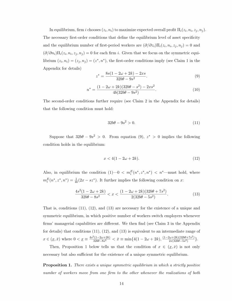
In equilibrium, firm i chooses (zi, ni) to maximize expected overall profit Πi(zi, ni, zj , nj).

The necessary first-order conditions that define the equilibrium level of asset specificity

and the equilibrium number of first-period workers are (∂/∂zi)Πi(zi, ni, zj , nj) = 0 and

(∂/∂ni)Πi(zi, ni, zj , nj) = 0 for each firm i. Given that we focus on the symmetric equi-

librium (zi, ni) = (zj , nj) = (z∗, n∗), the first-order conditions imply (see Claim 1 in the

Appendix for details)

z∗ =8s(1− 2ω + 2k)− 2xs

32bθ − 9s2. (9)

n∗ =(1− 2ω + 2k)(32bθ − s2)− 2xs2

4b(32bθ − 9s2). (10)

The second-order conditions further require (see Claim 2 in the Appendix for details)

that the following condition must hold:

32bθ − 9s2 > 0. (11)

Suppose that 32bθ − 9s2 > 0. From equation (9), z∗ > 0 implies the following

condition holds in the equilibrium:

x < 4(1− 2ω + 2k). (12)

Also, in equilibrium the condition (1)—0 < mEi (n∗, z∗, n∗) < n∗—must hold, where

mEi (n∗, z∗, n∗) = 1

4b(2x− sz∗). It further implies the following condition on x:

4s2(1− 2ω + 2k)

32bθ − 8s2< x <

(1− 2ω + 2k)(32bθ + 7s2)

2(32bθ − 5s2). (13)

That is, conditions (11), (12), and (13) are necessary for the existence of a unique and

symmetric equilibrium, in which positive number of workers switch employers whenever

firms’ managerial capabilities are different. We then find (see Claim 3 in the Appendix

for details) that conditions (11), (12), and (13) is equivalent to an intermediate range of

x ∈ (x, x̄) where 0 < x ≡ 4s2(1−2ω+2k)32bθ−8s2 < x̄ ≡ min{4(1− 2ω + 2k), (1−2ω+2k)(32bθ+7s2)

2x(32bθ−5s2) }.

Then, Proposition 1 below tells us that the condition of x ∈ (x, x̄) is not only

necessary but also sufficient for the existence of a unique symmetric equilibrium.

Proposition 1. There exists a unique symmetric equilibrium in which a strictly positive

number of workers move from one firm to the other whenever the realizations of both

14

firms’ managerial capabilities are different in period 2, if and only if x ∈ (x, x̄). The

equilibrium is characterized by each firm i’s level of asset specificity and number of first-

period workers (zi, ni) = (z∗, n∗) =(8s(1−2ω+2k)−2xs

32bθ−9s2 , (1−2ω+2k)(32bθ−s2)−2xs24b(32bθ−9s2)

).

Proposition 1 can be understood as follows. If the difference between high and low

managerial capability is too small, labor mobility will not occur since the workers in the

firm facing low capability still have relatively high productivity once been retained. If

the difference between high and low managerial capability is too large, a firm under-

went contraction will completely shut down given that the productivity of its workers is

relatively high in its rival firm.

Also note that in equilibriummEi (n∗, z∗, n∗) = mC

i (z∗, n∗, n∗) ≡ m∗ and wCi,2(z∗, n∗, n∗) =

wE−j,2(n∗, z∗, n∗) ≡ wSwitch2 , and let wEi,2(n

∗, z∗, n∗) ≡ wRetain2 and wi,1(z∗, n∗, z∗, n∗) ≡

w∗1. Then, in the equilibrium each firm chooses the level of asset specificity z∗, makes

first-period wage offer w∗1 to hire n∗ workers at Stage 1. At Stage 3 if both firms have

different managerial capabilities, firm i who realizes higher managerial capability retains

all its first-period employees at wage wRetain2 and expands in its firm size by hiring m∗

workers from firm j (j 6= i) at wage wSwitch2 , whereas firm j contracts in its firm size

and retains n∗ − m∗ workers at second-period wage wSwitch2 . Hence if ai 6= aj , there

exists a strictly positive number of workers, m∗, moving from the low-capability firm to

the high-capability firm in the equilibrium. At Stage 3 if ai = aj , each firm i retains

all its first-period workers at the second-period wage wSi,2(ai, n∗) and stays unchanged

in its firm size; thus there is no labor mobility. Then, the expected number of workers

who switch their employers at the beginning of period 2 is 14(2m∗), and each firm i’s

expected labor turnover rate is 14

(2m∗

n∗

)in the equilibrium.

We will now turn to comparative statics on the equilibrium level of the asset speci-

ficity z∗ and the firm size n∗, and the expected equilibrium turnover rate 14

(2m∗

n∗

). Note

that the period 1 number of workers n∗ can be interpreted as average firm size measured

by employment since n∗ determines each firm’s expected number of workers over two

periods.

Proposition 2. As the importance of managerial capability (captured by x) increases,

the level of asset specificity decreases, the average firm size decreases, and the expected

labor turnover rate increases in the equilibrium.

15

The key result here is that, as the importance of managerial capability increases,

the expected number of workers who switch their employers (expected labor mobility)

in period 2 becomes larger, and each firm’s asset specificity and average employment

size decreases. The logic behind this result can be explained as follows. When firm i

chooses the level of its asset specificity and the number of workers it employs in period

1, it estimates the expected number of its first-period employees that the firm will retain

for second-period operation, and the expected number of workers that the firm hires

from its rival firm j in period 2. A higher importance of managerial capability increases

the difference of period 2 productivity between a high-capability and a low-capability

firm. Then, as the importance of managerial capability increases, each firm anticipates

a larger number of workers switch their employers in period 2 if both firms’ managerial

capabilities turn out to be different. Hence a higher importance of managerial capability

decreases the expected number of retained workers, and it increases the expected number

of workers who switch employers. Holding the initial number of workers constant, this

reduces each firm’s incentive to choose higher specificity of its asset. This is because

higher firm-specificity increases a worker’s period 2 productivity only if the worker was

employed by the same firm in period 1 to be familiarized with the nature of the firm-

specificity.

Lower firm-specificity of asset, in turn, reduces each firm’s incentive to hire workers

in period 1 through two channels. First, lower firm-specificity reduces period 2 output

of a retained worker. Second, lower firm-specificity increases the fraction of workers

who switch employers in period 2 if the two firms realize different managerial capability.

These two effects together reduce the expected period 2 productivity of each period 1

worker, implying that the number of workers employed by each firm in period 1 decreases

as the importance of managerial capability increases. The last result of Proposition 2

naturally follows from the key result mentioned above. As the importance of managerial

capability increases, the expected labor turnover rate, measured by the ratio of expected

number of workers who switch their employers in period 2 to the number of first-period

workers, increases unambiguously in the equilibrium.

Proposition 3. As the importance of a firm’s asset specificity (captured by s) increases,

the level of asset specificity increases, the average firm size increases, and the expected

labor turnover rate decreases in the equilibrium.

16

Recall that in period 1 firm i estimates the number of workers it will retain and

hire from the rival firm in period 2, respectively. As the importance of firm i’s asset

specificity increases, firm i will retain more of its first-period employees during the

contraction phase, while hire fewer workers from its rival during the expansion phase

since new workers become relatively less productive in firm i. This implies that each

firm anticipates a smaller number of workers switch their employers in period 2 if the

realized managerial capabilities are different. Lower expected labor mobility, along with

the higher return from retained workers (captured by s), implies that a firm has higher

incentive to choose a higher level of asset specificity. These two effects are mutually

reinforcing because the higher level of asset specificity reduces the expected turnover

rate by increasing the retained workers’ productivity. The results of the average firm

size and expected turnover rate follow through the logic analogous to the one explained

for Proposition 2.

5 Discussion

5.1 An application to the TCE prediction on uncertainty

Our theoretical framework enriches a prediction of TCE on the relationship between

uncertainty and governance structure. As mentioned in Introduction, a standard pre-

diction of TCE is that, in line with asset specificity and frequent transactions, higher

uncertainty makes vertical integration more likely.

Our model incorporates uncertainty of each firm’s managerial capability, where the

degree of uncertainty increases as the importance of managerial capability shock in-

creases. A key prediction of our model can then be restated in terms of uncertainty

as follows: Higher uncertainty increases labor mobility, which in turn reduces the de-

gree of each firm’s asset specificity. Then, applying another standard prediction of TCE

that higher degree of asset specificity makes vertical integration more likely, our model

implies a mediation process where the uncertainty (exogenous variable) affects vertical

integration through asset specificity (an intermediate variable or a mediator).

17

Consider estimating the following structural equations with such mediation process:

Yi = β0 + β1Mi + β2Xi + εi1, (14)

Mi = γ0 + γ1Xi + εi2, (15)

where Xi and Mi represents the observed level of uncertainty and asset specificity, re-

spectively, and Yi is the observed vertical integration choice.6 In this mediation process,

the total effect of the uncertainty can be decomposed into direct and indirect effects.

The direct effect equals the effect of uncertainty on vertical integration choice that is not

transmitted by the mediator—asset specificity. This direct effect thus corresponds to

the TCE prediction where the coefficient β2 is positive. On the other hand, our model

points out that there exists an indirect effect of the uncertainty on vertical integration

going through asset specificity, in which the coefficient γ1 is negative. The total ef-

fect of the uncertainty on vertical integration thus equals β2 + γ1β1. Notice that TCE

predictions also require β1 be positive. Hence, the sign of β2 + γ1β1 is indeterminate.

When uncertainty’s (negative) indirect effect outweighs its (positive) direct effect, our

model predicts that uncertainty makes vertical integration less likely. This prediction is

opposite to the standard TCE prediction. The structural equations thus imply a richer

relationship between uncertainty and governance structure.

Another implication of this setting is that it highlights a twofold estimation chal-

lenge. First, an endogeneity problem exists in a regression model if only asset specificity

is included in the explanatory variables. A similar point has been made by Macher and

Richman (2008)’s empirical TCE review article. They state “Virtually all of the [em-

pirical] studies examined in this survey treat the specificity of assets and the level of a

firm’s investment in those assets as exogenous. These are, however, choice variables ...

should therefore be treated as endogenous.” Here we identify one cause (i.e., exclusion

of uncertainty) of such endogeneity of asset specificity.

Second, if the underlying regression model has the structure as in equations (14)

and (15), estimating uncertainty effect in a single linear regression model with asset

specificity included in explanatory variables as in equation (14) (i.e., without considering6The key identification assumption for such causal mechanism, a process in which a causal variable

of interest influences the outcome, is error terms εi1 and εi1 are uncorrelated. See Imai, Keele andYamamoto (2010) and Imai, Keele, Tingley and Yamamoto (2011) for the proofs and discussions underwhich γ̂1β̂1 is a valid estimator (i.e., asymptotically consistent) of the indirect (mediation) effect.

18

the indirect effect of uncertainty) results in multicollinearity problem. Because there is a

linear relationship between uncertainty and asset specificity. Consequently, the resulting

estimate can be either imprecise or numerically inaccurate even though it is not biased.

Our structural equations thus reconcile the seemingly mixed results of uncertainty effect

on vertical integration in TCE empirical literature.7

Specificially, Lieberman (1991) finds in his study of chemical products that volatility

in the firm’s downstream detrended market sales appears to have little influence on

integration decisions. Anderson and Schmittlein (1984) find in their study of the electric

components industry, “Contrary to the transaction cost model, neither frequency of

transactions nor interaction of specificity and environmental uncertainty [forecast error

in sales] is significantly related to integration.” By using data from multiple industries,

Norton (1988) finds in the industries of motels and refreshment places that detrended

percentage variations in retail sales have negative effect on integration choice, in which

the negative effect in the latter industry is significant. Notice that the studies referred to

above adopt the variance of detrended sales or of forecasting errors or the instability of

market shares as their empirical measures for uncertainty.8 This uncertainty measure is

consistent with our model environment since our model predicts that higher uncertainty

results in higher labor mobility, leading to higher volatility of market share. But these

empirical studies, in fact, test the TCE prediction that β2 is positive, ignoring the

indirect channel that our model identifies. As a result, their estimates are imprecise and

may have sizable change due to high degree of multicollinearity. Also, the insignificant

or negative sign of their uncertainty coefficient, despite not lending support to TCE

prediction on the surface, can still be compatible under our setup.

5.2 An application to different phases of an industry’s life cycle

The second application concerns the idea that the importance of managerial capability

shock can differ as an industry goes through stages of its life cycle (Helfat and Peteraf,

2003). For example, as an industry evolves from infancy stage, firms typically undergo7For review articles, see Shelanski and Klein (1995); Lafontaine and Slade (2007); Macher and

Richman (2008). As argued by Macher and Richman (2008), although TCE predictions have earnedempirical success in many of its central tenets, several prior empirical studies do not lend support tothe role of uncertainty in the decision of vertical integration.

8This type of uncertainty measure, as mentioned by Lafontaine and Slade (2007), is common in theempirical literature.

19

revolutionary technological changes that is characterized by Schumpeter’s “creative de-

struction” (Agarwal, Sarkar and Echambadi, 2002; Winter, 1984). Thus, a business’s

success critically depends on the quality of its strategic decision making because firms

during this stage are surrounded by a high level of uncertainty about the needs of cus-

tomers, the products and services that will prove to be the most desired, and the best

configuration of activities and technologies to deliver them. Whereas in the mature phase

of an industry, institutional structures become clear and the opportunity for radical in-

novation is few. It follows that firms during this stage face lower level of uncertainty,

and thus strategic decision making is less important for them.9 These arguments suggest

that the importance of managerial capability shock is higher during the early phase of

an industry’s life cycle with revolutionary technological changes and higher level of un-

certainty, while the degree tends to be lower in the mature phase of an industry with less

technological advancement and lower level of uncertainty. Our model then predicts that

labor mobility is higher, specificity of asset and human capital is lower, and average firm

size is smaller in the early or growing phases of an industry’s life cycle and vice-versa in

the later or mature phases.

These predictions are consistent with empirical and observational evidence. Concern-

ing firm size, Dinlersoz and MacDonald (2009) show that average firm size, measured

by employment (but not output), in U.S. manufacturing industries from 1963 until 1997

falls over time during the rapid entry phase of the industry’s life-cycle, where the rapid

entry phase occurs during the first stage of life cycle and when there exists greater

technological improvement. In addition, using manufacturing firm data from Portugal,

Italy, and Spain, respectively, Cabral and Mata (2003), Angelini and Generale (2008),

and Segarra and Teruel (2012) all confirm that the firm size distribution of employees

clearly skewed to the right (most of the mass is on small firms) and the skewness tends to

diminish with firm age.10 That is, the smaller the firm size, the younger the firm. Since

young firms account for a much higher fraction in the starting stages of an industry’s9See also empirical study by Katila and Shane (2005). Using data on firms’ efforts to commercialize

technological inventions, they find that firms’ innovation activity in response to market competitivenessdiffers depending on firm newness. Giving that entries of new firms occur mostly during the early stageof an industry’s life cycle, this finding suggests that the importance of managerial capability shockdiffers across different life cycle stages.

10Cabral and Mata (2003) consider the cohort of firms that entered Portuguese manufacturing in 1984and follow them until 1991. Angelini and Generale (2008) study the firm size distribution of employeesby pooling Italian manufacturing firm data in 1992, 1995, 1998, and 2001. Segarra and Teruel (2012)use Spanish manufacturing firms data in both 2001 and 2006.

20

life cycle, this result also implies average firm size tends to be smaller during the earlier

life cycle stages.

Concerning labor mobility, Benner (2002) studies labor markets in Silicon Valley

and points out that, “The rapid turnover and volatility in employment in Silicon Val-

ley is integrally connected to the nature of competition in the region’s high-technology

industries. In these industries, markets and technology change extremely rapidly and

in unpredictable ways.” Notice that, compared with U.S. automobile industry, Silicon

Valley is considered as high-tech clusters consisting of relatively young firms or star-

tups with concentrated entrepreneurship,11 reflecting a growing stage of the industry

evolution.

5.3 An application to U.S.-Japanese differences

The U.S. and Japan have been considered representing two contrasting employment

systems, which attracts significant attention in the literature of international comparison

in how internal labor markets operate. By capturing the interconnections among asset

specificity, acquisition of firm-specific human capital, managerial capability, and labor

mobility, our model offers new explanations for and predictions on the U.S.-Japanese

differences based on the cross-country differences in the importance of both managerial

capability and firm-specificity of asset.

Acemoglu, Aghion and Zilibotti (2006) argue in their analysis of technology frontiers

and firm selection that managerial skill is more important for undertaking innovative ac-

tivities than for adopting and imitating existing technologies from the world technology

frontier. They then point out, based on their analysis of the correlation between distance

to the frontier and R&D intensity using data from the OECD sectoral database, that

innovation becomes more important as the economy approaches the world technology

frontier and there remains less room for adoption and imitation. Following their analysis

and argument, we argue that the importance of managerial capability was substantially

lower in Japan than in the U.S. when most Japanese industries were catching up with

the West in the postwar growth period (Okimoto, 1989).

On the other hand, as the economy makes the transition from industrial capitalism11Zhang (2003) shows that, in Silicon Valley, more than half of the 2002 top 40 technology companies

were not even founded two decades ago.

21

to post-industrial capitalism, modern economies are becoming increasingly knowledge

intensive which renders the disadvantage to the firms that heavily rely on physical assets.

For example, Iwai (2002) points out that, in the new era of post-industrial capitalism, the

physical assets have surrendered their central position to the knowledge-based human

assets that money can no longer buy and control.12 The advent of knowledge economy

thus reduces the importance of firm-specificity of asset across the world. But different

countries have different paths in making their transition to the knowledge economy.

Based on the knowledge assessment methodology (KAM) developed by World Bank

Institute that traces the challenges and opportunities of major economies’ transition to

knowledge-based economy from 1995, the U.S. has a better shape than Japan in their

development of knowledge economy (Shibata, 2006). Following this reasoning, we argue

that the importance of firm-specificity of asset is higher in Japan than in the U.S.

Combining the above argument where Japan has lower importance of managerial

capability and higher importance of firm-specificity of asset compared with U.S., the

predictions of our model point out to the same direction. That is, labor mobility was

lower, and specificity of asset and human capital was higher in Japan than in the U.S.,

especially in the catching up period.13

These predictions are consistent with empirical and observational evidence. Concern-

ing labor mobility, it was found that the labor turnover rate was much higher in U.S.

than in Japan (see Hashimoto and Raisian, 1985; Mincer and Higuchi, 1988). Hashimoto

and Raisian (1985), for instance, found that the 15-year job retention rates of the male

population between the early 1960s and the late 1970s were much higher in Japan than in

the United States across all age groups. Concerning firm-specific human capital, Koike

(1977, 1988) found, in his comparative analysis of Japanese and U.S. industrial rela-

tions, that Japanese workers acquired more firm-specific human capital through rotation

among related jobs (see also Dertouzos, Lester and Solow, 1989; Ito, 1991). Concerning12Also, Drucker (1993) for example, has argued that in the new economy, knowledge is not just

another resource alongside the traditional factors of production—labor, capital, and land—but the onlymeaningful resource today.

13In an alternative approach where promotion serves as a signal of the worker’s ability, Owan (2004)shows that late-promotion practice which commonly observed in Japanese firms results in low turnoverrate and long-term employment relationship; whereas early-promotion practice which is commonly ob-served in U.S. results in the opposite effects. Moreover, Chang and Wang (1995) explain the lowerturnover rate and higher human capital accumulation in Japan than in the U.S. Their model is charac-terized by multiple equilibria and is analyzed in the framework where current employers have superiorinformation on the abilities of their employees.

22

specificity of asset, we are unaware of direct observations or evidence. However, it is

well known that Japanese firms conducted continuous process improvement more than

U.S. firms did in the postwar growth period.14 As argued by Morita (2001), if a firm

conducts continuous process improvement, the technology is improved but a degree of

specificity is introduced. This is because, in general, continuous process improvement

involves a number of small changes and modifications, which lead to highly firm-specific

technologies. This then suggests that specificity of asset was higher in Japanese firms

than in the U.S. firms in the postwar growth period.

The Japanese economy has already caught up with the West, and most Japanese

industries have got much closer to the world technology frontier. This increases the

importance of managerial capability in which undertaking innovative activities now be-

comes crucially sensitive to higher managerial capability. Our model then predicts that

the degree of the U.S.-Japanese differences become smaller. That is, labor mobility had

increased, and specificity of asset and human capital has decreased in Japan. In reality,

however, such transitions in Japan are likely to take place rather slowly due to vested

interests and institutional inertia embedded in the Japanese economic system (Lincoln,

2001). Several empirical studies have been undertaken recently to find out whether or

not the Japanese employment system has exhibited significant changes, but findings are

not clear-cut thus far.15

6 Conclusion

We have developed a model of labor market competition that captures the link between

capability of a firm’s top management, specificity of a firm’s asset, and firm-specificity of

human capital. Firm-specificity of asset is a key concept in the RBV of the firm and TCE,

and distinction between general and firm-specific human capital has played an important

role in the human capital theory literature. We have contributed to these literatures by

proposing a model in which the degree of firm-specificity is endogenously determined,14See Morita (2001) for a review of evidence.15For example, Kambayashi and Kato (2017) study labor mobility and conduct cross-national analysis

of micro data from Japan Employment Status Survey and U.S. Current Population Survey. They findthat, on the one hand, core employees (age of 30-44 with at least five years of tenure) in Japan continuedto enjoy much higher job stability than the U.S. counterparts consistently over the last twenty-five years.On the other hand, job stability for mid-career hires and youth employees deteriorated in Japan over thelast twenty-five years, whereas there was no comparable decline in job stability in the U.S. counterparts.

23

where labor mobility generated by ex ante uncertainty of managerial capabilities and

the link between firm-specificities of asset and human capital are the driving forces

of the endogenous determination. Furthermore, our theoretical framework enriches a

prediction of TCE on the relationship between uncertainty and governance structure by

indicating that higher uncertainty can make vertical integration less likely. Given that

the importance of managerial capability differs across industries, countries and time,

our theoretical results yield empirical implications and predictions from a previously

unexplored perspective.

24

Appendix

Proof of Proposition 1:

Suppose that there exists a symmetric equilibrium characterized by (zi, ni) = (z∗, n∗)

for each i, in which a strictly positive number of workers switch employers in period 2

whenever the realizations of managerial capability are different in both firms. In the

text, it has been shown that conditions (11), (12), and (13) are necessary for such an

equilibrium to exist. Here, in Claim 1–3 below, we present proof of some computational

details that have not been presented in the text.

Claim 1: In a symmetric equilibrium where a strictly positive number of workers

switch employers in period 2 whenever the realizations of managerial capability are dif-

ferent in both firms, each firm i chooses zi = z∗ = 8s(1−2ω+2k)−2xs32bθ−9s2 and ni = n∗ =

(1−2ω+2k)(32bθ−s2)−2xs24b(32bθ−9s2) .

Proof of Claim 1: Suppose that there exists an equilibrium in which a strictly positive

number of workers switch employers in period 2 when firms’ managerial capabilities

are different. First notice that in the Stage 3 subgame, firm i’s second-period profit

conditional on ai = k + x and ai 6= aj is πEi (zi, ni, zj , nj) = ni(k + x + 1 + szi) +

mEi (ni, zj , nj)(k+x+1)−b(ni+mE

i (ni, zj , nj))2−(niw

Ei,2(ni, zj , nj)+m

Ei (ni, zj , nj)w

E−i,2(ni, zj , nj))

as analyzed in the text, implying that

πEi (zi, ni, zj , nj) =1

16b{4[(b(ni + nj) + x)2 + 4bsnizi

](16)

+4s(3bni − bnj − x)zj + (szj)2},

given mEi (ni, zj , nj) = 1

4b [2x−szj−2b(ni−nj)], wEi,2(ni, zj , nj) = 12 [2+2k−szj−2b(ni+

nj)], and wE−i,2(ni, zj , nj) = 12 [2 + 2k + szj − 2b(ni + nj)]. Second notice that, if firm i

contracts and firm j expands, the equilibrium size of of expansion/contraction can be

solved analogously, which is 14b [−2x−szj−2b(ni−nj)]. This case where firm i contracts

and firm j expands can be ruled out since −2x−szj−2b(ni−nj) < 0 for any symmetric

equilibrium—a contradiction. Third, it cannot be the case that firm i retains only some

of its period 1 employees and firm j (j 6= i) hires some workers from i in the equilibrium.

The reason is as follows. Suppose firm i retains ni − li of its period 1 employees, where

li > 0, and hire ri(> 0) workers from firm j in which the size of the expansion is positive

25

and equals ri − li; firm j retains nj − rj of its period 1 employees, where rj > 0, and

hire lj(> 0) workers from firm i in which the size of contraction is rj − lj . Then, firm

i offers k + x + 1 − 2b(ni + ri − li) ≡ wEi,O to hire ri outside workers and firm j offers

k−x+1+szj−2b(nj−rj+lj) ≡ wCj,R to retain nj−rj of its period 1 employees, in which

wEi,O = wCj,R and the size of expansion ri−li ≡ mi equals that of contraction rj−lj ≡ −mj

in equilibrium. We have mi = −mj = 14b [2x− szj − 2b(ni − nj)]. Similarly, firm i offers

k+x+1+szi−2b(ni+ri− li) ≡ wEi,R to retain ni− li of its period 1 employees and firm j

offers k−x+1−2b(nj−rj+lj) ≡ wCj,O to hire lj outside workers, in which wEi,R = wCj,O in

equilibrium. The implied expansion/contraction size in equilibrium from this later case is14b [2x+szi−2b(ni−nj)]. Given that 1

4b [2x−szj−2b(ni−nj)] 6= 14b [2x+szi−2b(ni−nj)] for

any symmetric equilibrium, firm i (expansion firm) will retain all its period 1 employees.

Consider the Stage 3 subgame where (ai, aj) = (x−k, k+x). If firm i contracts and

firm j expands in their firm sizes, firm i makes offers wii = k−x+1+szi−2b(ni+mi) to

retain ni+mi (mi < 0) workers from its period 1 employees where k−x+1+szi−2b(ni+

mi) is the expected productivity of firm i’s first-period employee in i given ni+mi of them

are retained. While firm j is willing to offer wji = k+x+1−2b(nj+mj) to hire mj(> 0)

new workers, where k+ x+ 1− 2b(nj +mj) equals the expected productivity of firm i’s

first-period employees in firm j. In the equilibrium, both firms offer the same second-

period wage to the workers in firm i such that wii = wji, and the number of workers

from contraction equals that from expansion, −mi = mj ≡ mCi (zi, ni, nj). We obtain

mCi (zi, ni, nj) = 1

4b [2x−szi+2b(ni−nj)]. Then, the equilibrium second-period wage for

workers retained in firm i and newly hired in firm j becomes 12 [2+2k+szi−2b(ni+nj)] ≡

wCi,2(zi, ni, nj). Notice that, if firm i expands and firm j contracts in the equilibrium, the

expansion/contraction size is 14b [−2x− szi + 2b(ni−nj)]. This equilibrium can be ruled

out given −2x− szi + 2b(ni − nj) < 0 for any symmetric equilibrium—a contradiction.

Further notice that, 0 < mCi (zi, ni, nj) < ni holds in the equilibrium, which suggests

0 < 14b [2x − szi + 2b(ni − nj)] < ni. This condition is the same as the condition (1) in

the equilibrium. Lastly, notice that firm i will not hire some of firm j’s workers while

maintaining the contraction size, mCi (zi, ni, nj), in the equilibrium. Because this does

not hold for symmetric equilibrium as analyzed in the previous paragraph. Then, firm i’s

second-period profit conditional on ai = k−x is πCi (zi, ni, nj) = (ni−mCi (zi, ni, nj))(k−

26

x+ 1 + szi)− b(ni−mCi (zi, ni, nj))

2− (ni−mCi (zi, ni, nj))w

Ci,2(zi, ni, nj), implying that

πCi (zi, ni, nj) =1

16b[2x− szi − 2b(ni + nj)]

2. (17)

Next consider the Stage 3 subgame where both firms have the same managerial

capabilities, ai = aj . First note that it cannot be the case that one firm expands and

the other contracts given that either −szj + 2b(ni − nj) ≯ 0 or −szi + 2b(nj − ni) ≯ 0

(the gap of realized managerial capability is now 0) under symmetric equilibrium. Then,

both firms must stay unchanged in their firm sizes in the equilibrium. That is, each firm

i will offer the wage to the extent that the expected productivity from the outside

workers are the same at the level ai + 1 − 2b(ni + mi) where mi = 0 holds in the

equilibrium. That is, each firm i make offers wSi,2(ai, ni) = ai + 1− 2bni to retain all of

its first-period employees. Then firm i’s second-period profit conditional on ai = aj is

πSi (zi, ni) = ni(ai + 1 + szi)− bn2i − niwSi,2(ai, ni), implying that

πSi (zi, ni) = ni(szi + bni). (18)

Consequently, in the equilibrium each firm i’s expected profit in period 2 is πi,2(zi, ni, zj , nj) =

Pr(ai > aj)πEi (zi, ni, zj , nj) + Pr(ai < aj)π

Ci (zi, ni, nj) + Pr(ai = aj)π

Si (zi, ni), where

Pr(ai > aj) = Pr(ai < aj) = 14 and Pr(ai = aj) = 1

2 .

Also, wi,1 + E[wi,2(zi, ni, zj , nj)] = 2ω holds for a worker employed by firm i in

the equilibrium where E[wi,2(zi, ni, zj , nj)] = Pr(ai > aj)wEi,2(ni, zj , nj) + Pr(ai <

aj)wCi,2(zi, ni, nj) + Pr(ai = aj)w

Si,2(ai, ni) and 2ω is the lifetime wage for self-employed

individuals. Note that wCi,2(zi, ni, nj) = wE−j,2(zi, ni, nj) so that the second-period

wage of the new workers who are hired by expansion firm is actually determined by

contraction firm’s strategic variables. By substituting the value of wEi,2(zi, ni, zj , nj),

wCi,2(zi, ni, zj , nj), and wSi,2(ai, ni), we obtain

E[wi,2(zi, ni, zj , nj)] = 1 + k +1

8[s(zi − zj)− 4b(3ni + nj)]. (19)

Then, we find wi,1 = wi,1(zi, ni, zj , nj) where

w∗i,1(zi, ni, zj , nj) = 2ω − (1 + k)− 1

8[s(zi − zj)− 4b(3ni + nj)]. (20)

27

Hence, each firm i’s expected overall profit is Πi(zi, ni, zj , nj) = niE(ai) − bn2i −12θz

2i −Wi,1 + π2(zi, ni, zj , nj), implying that

Πi(zi, ni, zj , nj) = ni[k + E(xi)− bni − w1(zi, ni, zj , nj)]−1

2θz2i (21)

+1

4πEi (zi, ni, zj , nj) +

1

4πCi (zi, ni, nj) +

1

2πSi (zi, ni)

=1

64b{{−8b2(5ni − nj)(3ni + nj) + 8x2 − 4sx(zi + zj) + s2(z2i + z2j )

+4b[snj(zi − zj) + ni(16− 32ω + 15szi + szj + 32k)− 8θz2i ]},

where πEi (zi, ni, zj , nj), πCi (zi, ni, nj), and πSi (zi, ni) are defined in the equations (16),

(17), and (18) respectively. Let compute the partial derivatives of Π(zi, ni, zj , nj). We

find

(∂/∂zi)Πi(zi, ni, zj , nj) =s

32b[2b(15ni + nj)− 2x+ szi]− θzi,

(∂/∂ni)Πi(zi, ni, zj , nj) = 1− 2ω + 2k +1

16[15szi + szj − 4b(15ni + nj)].

Given that (zi, ni) = (zj , nj) = (z∗, n∗) in the symmetric equilibrium, the first-order

conditions imply (s

32b

)(sz∗ − 2x) + (sn∗ − θz∗) = 0

1− 2ω + 2k + sz∗ − 4bn∗ = 0

. (22)

Solving the simultaneous equations, we obtain z∗ = 8s(1−2ω+2k)−2xs32bθ−9s2 and n∗ = (1−2ω+2k)(32bθ−s2)−2xs2

4b(32bθ−9s2)

in the equilibrium. �

Claim 2: In a symmetric equilibrium where a strictly positive number of workers switch

employers in period 2 whenever the realizations of managerial capability are different

in both firms, condition (11) presented in the text is necessary for each firm i’s choice

(zi, ni) = (z∗, n∗).

Proof of Claim 2: Let us check the second-order condition of firm i’s maximization prob-

lem over its profit function Πi(zi, ni, zj , nj) to rule out candidate critical point under dif-

ferent parameterization. We have (∂2/∂z2i )Πi(zi, ni, zj , nj) = s2

32b−θ, (∂2/∂n2i )Πi(zi, ni, zj , nj) =

−154 b, and (∂2/∂zi∂ni)Πi(zi, ni, zj , nj) = (∂2/∂ni∂zi)Πi(zi, ni, zj , nj) = 15

16s. Hence, the

first-order leading principal minor of D2Πi(zi, ni, zj , nj) is negative and the second-order

28

leading principal minor ofD2Πi(zi, ni, zj , nj) is 15128(32bθ−8.5s2). That is,D2Πi(zi, ni, zj , nj)

is negative definite over all zi ≥ 0 and ni ≥ 0 if 32bθ − 8.5s2 > 0. We need to show

that there does not exist a range of parametrization for the existence of symmetric

equilibrium such that 8.5s2 < 32bθ < 9s2 holds for the solution z∗ > 0 and n∗ > 0.

Suppose 8.5s2 < 32bθ < 9s2 holds. Then given that the denominator of z∗ is

negative, x ≥ 4(1 − 2ω + 2k) implies 1 − 2ω + 2k > 0 must hold. Also, given 0 <

mEi (n∗, z∗, n∗) < n∗ where mE

i (n∗, z∗, n∗) = 14b(2x− sz

∗), we have (1−2ω+2k)(32bθ+7s2)2(32bθ−5s2) <

x < 4s2(1−2ω+2k)32bθ−8s2 . Notice that (32bθ+7s2)

2(32bθ−5s2)−4s2

32bθ−8s2 = (32bθ)2−288bθs2−16s42(32bθ−5s2)(32bθ−8s2) = (32bθ−8s2)(32bθ−2s2)+32bθs2

2(32bθ−5s2)(32bθ−8s2) >

0 given 32bθ − 8.5s2 > 0. That is, the range of x satisfying (1−2ω+2k)(32bθ+7s2)2(32bθ−5s2) < x <

4s2(1−2ω+2k)32bθ−8s2 is an empty set. We thus complete the proof. �

Claim 3: For any given parameterization, there exists unique values x̄ and x, respec-

tively, such that conditions (11), (12), and (13) hold if and only if x ∈ (x, x̄). There

exists a range of parameterizations in which 0 < x < x̄.

Proof of Claim 3: Suppose x < 4(1 − 2ω + 2k) so that condition (12) holds. Then,

4(1 − 2ω + 2k) > 0 must hold. Using condition (11) and 4(1 − 2ω + 2k) > 0, we have

4(1 − 2ω + 2k) > 4s2(1−2ω+2k)32bθ−8s2 . Concerning the case where x < (1−2ω+2k)(32bθ+7s2)

2(32bθ−5s2) so

that the RHS of inequality (13) holds. We find (1−2ω+2k)(32bθ+7s2)2(32bθ−5s2) − 4s2(1−2ω+2k)

32bθ−8s2 =

(1−2ω+2k)2(32bθ−5s2)(32bθ−8s2) [(32bθ)2 − 288bθs2 − 16s4] = (1−2ω+2k)

2(32bθ−5s2)(32bθ−8s2) [(32bθ− 8s2)(32bθ−

2s2) + 32bθs2] > 0, given condition (11) and 4(1 − 2ω + 2k) > 0. Let x ∈ (x, x̄) where

x̄ = min{4(1 − 2ω + 2k), (1−2ω+2k)(32bθ+7s2)2x(32bθ−5s2) } and x = 4s2(1−2ω+2k)

32bθ−8s2 such that the range

of x satisfying this condition is non-empty. Note that 4s2(1−2ω+2k)32bθ−8s2 > 0. This implies

the result. �

Claim 1–3, along with the analysis presented in the text, imply the following nec-

essary part of the proposition: “Suppose that there exists a unique symmetric equilib-

rium in which a strictly positive number of workers move from one firm to the other

whenever the realizations of both firms’ managerial capabilities are different in period

2. Then x ∈ (x, x̄) where 0 < x < x̄ must hold.” We now check sufficiency. Sup-

pose that 0 < x < x < x̄ holds, and that each firm i chooses (zi, ni) = (z∗, n∗) =(8s(1−2ω+2k)−2xs

32bθ−9s2 , (1−2ω+2k)(32bθ−s2)−2xs24b(32bθ−9s2)

). First note that z∗ > 0 and n∗ > 0 hold given

0 < x < x < x̄. Then, following the procedure in the text and Claim 1, firm i’s optimal

29

decision in period 2 is to expand in its firm size if (ai, aj) = (k + x, k − x), to contract

in its firm size if (ai, aj) = (k − x, k + x), and to stay unchanged in its firm size if

ai = aj . This is the case if the condition (1) (0 < 14b [2x− szj − 2b(ni−nj)] < nj) holds,

suggesting each firm i’s expected overall profit at Stage 1 is Πi(zi, ni, zj , nj). Notice

that, 0 < 14b [2x − szj − 2b(ni − nj)] < nj holds true for (zi, ni) = (zj , nj) = (z∗, n∗).

That is, if 0 < x < x ≤ x̄, there exists a symmetric equilibrium with the following prop-

erties: (i) (zi, ni) = (z∗, n∗) =(8s(1−2ω+2k)−2xs

32bθ−9s2 , (1−2ω+2k)(32bθ−s2)−2xs24b(32bθ−9s2)

)where z∗ > 0

and n∗ > 0; (ii) at Stage 1, each firm chooses the level of asset specificity z∗ and makes

first-period wage offer w∗1 to n∗ individuals, and employs n∗ workers; (iii) at Stage 3 if

both firms have different managerial capabilities, firm i who realizes higher managerial

capability retains all its first-period employees at wage wRetain2 and expands in its firm

size by hiring m∗ workers from firm j (j 6= i) at wage wSwitch2 , whereas firm j contracts

in its firm size and retains n∗ −m∗ workers at second-period wage wSwitch2 ; if ai = aj ,

each firm i retains all its first-period workers at the second-period wage wSi,2(ai, n∗) and

stays unchanged in its firm size; (iv) the expected number of workers who switch their

employers at the beginning of period 2 is m∗ conditional on both firms have different

managerial capabilities.

Finally, if 0 < x < x < x̄, the symmetric equilibrium described in the previous

paragraph is also unique. Because the implied condition (11) (32bθ − 9s2 > 0) ensures

that Πi(zi, ni, z∗, n∗) is globally concave over all zi > 0 and ni > 0, and the only

solution satisfying both (∂/∂zi)Πi(zi, ni, z∗, n∗) = 0 and (∂/∂ni)Πi(zi, ni, z

∗, n∗) = 0

for each firm i is (zi, ni) = (z∗, n∗). This completes the proof of the proposition. �

Proof of Proposition 2 and 3:

(i) Note z∗ = 8s(1−2ω+2k)−2xs32bθ−9s2 , we find ∂z∗

∂x = −2s32bθ−9s2 < 0 given 32bθ − 9s2 > 0. Also,

∂z∗

∂s = [8(1−2ω+2k)−2x](32bθ−9s2)+[8s(1−2ω+2k)−2xs](18s)(32bθ−9s2)2 > 0 given 8s(1−2ω+ 2k)−2xs > 0

and 32bθ − 9s2 > 0.

(ii) Note n∗ = (1−2ω+2k)(32bθ−s2)−2xs24b(32bθ−9s2) , we find ∂n∗

∂x = −2s24b(32bθ−9s2) < 0. Also, ∂n∗

∂s =

32s[4(1−2ω+2k)−x](32bθ−9s2)2 > 0 given 8s(1− 2ω + 2k)− 2xs > 0.

(iii) Note m∗ = 14b(2x− sz

∗), we find ∂m∗

∂x = 14b(2− s

∂z∗

∂x ) > 0 given ∂z∗

∂x < 0. Then given∂n∗

∂x < 0 and ∂m∗

∂x > 0, we find ∂(142m∗

n∗ )/∂x = 1(2n∗)2 [∂m

∗

∂x (2n∗)−m∗(∂n∗∂x )] > 0. Also, we

30

find ∂m∗

∂s = − 14b

(z∗ + s∂z

∗

∂s

)< 0 given z∗ ≥ 0 and ∂z∗

∂s > 0. Then given ∂n∗

∂s > 0 and∂m∗

∂s < 0, we find ∂(142m∗

n∗ )/∂s = 1(2n∗)2 [∂m

∗

∂s (2n∗)−m∗(∂2n∗∂s )] < 0. �

31

References

Aaker, David, Great CEOs are Born, Not Made, Harvard Business Review, July 2011.

Acemoglu, Daron, Philippe Aghion, and Fabrizio Zilibotti, “Distance to Fron-

tier, Selection, and Economic Growth,” Journal of the European Economic Associa-

tion, 2006, 4 (1), 37–74.

Agarwal, Ratshree, MB Sarkar, and Raj Echambadi, “The Conditioning Effect

of Time on Firm Survival: An Industry Life Cycle Approach,” The Academy of Man-

agement Journal, 2002, 45 (5), 971–994.

Anderson, Erin and David C. Schmittlein, “Integration of the Sales Force: An

Empirical Examination,” The Rand Journal of Economics, 1984, 15 (3), 385–395.

Angelini, Paolo and Andrea Generale, “On the Evolution of Firm Size Distribu-

tions,” American Economic Review, 2008, 98 (1), 426–38.

Bai, Chong-En and Yijiang Wang, “Uncertainty in Labor Productivity and Specific

Human Capital Investment,” Journal of Labor Economics, 2003, 21 (3), 651–675.

Barney, Jay, “Firm Resources and Sustained Competitive Advantage,” Journal of Man-

agement, 1991, 17 (1), 99–120.

Becker, Gary S., “Investment in Human Capital: A Theoretical Analysis,” Journal of

Political Economy, 1962, 70 (5), 9–49.

Benner, Chris, Work in the New Economy: Flexible Labor Markets in Silicon Valley,

Malden, MA: Wiley, 2002.

Cabral, Luis and Jose Mata, “On the Evolution of the Firm Size Distribution: Facts

and Theory,” American Economic Review, 2003, 93 (4), 1075–1090.

Chang, Chun and Yijiang Wang, “A Framework for Understanding Differences in

Labor Turnover and Human Capital Investment,” Journal of Economic Behavior &

Organization, 1995, 28 (1), 91–105.

Denis, David J., Diane K. Denis, and Mark D. Walker, “CEO Assessment and

the Structure of Newly Formed Boards,” The Review of Financial Studies, 2015, 28

(12), 3338–3366.

32

Dertouzos, Michael L., Richard Lester, and Robert Solow, Made in America,

Cambridge, MA: MIT Press, 1989.

DeVaro, Jed and Hodaka Morita, “Internal Promotion and External Recruitment:

A Theoretical and Empirical Analysis,” Journal of Labor Economics, 2013, 31 (2),

227–269.

Dinlersoz, Emin M. and Glenn MacDonald, “The Industry Life-Cycle of the Size

Distribution of Firms,” Review of Economic Dynamics, 2009, 12 (4), 648–667.

Drucker, Peter F., Managing for the Future, London: Routledge, 1993.

Gabaix, Xavier and Augustin Landier, “Why has CEO Pay Increased So Much,”

The Quarterly Journal of Economics, 2008, 123 (1), 49–100.

Goleman, Daniel, “What Makes a Leader?,” Harvard Business Review, 1998, 76, 92–

102.

Hashimoto, Masanori and John Raisian, “Employment Tenure and Earnings Pro-

files in Japan and the United States,” The American Economic Review, 1985, 75 (4),

721–735.

Helfat, Constance E and Margaret A Peteraf, “The Dynamic Resource-Based

View: Capability Lifecycles,” Strategic Management Journal, 2003, 24 (10), 997–1010.

Hoopes, David G., Tammy L. Madsen, and Gordon Walker, “Guest Editors’

Introduction to the Special Issue: Why Is There a Resource-Based View? Toward a

Theory of Competitive Heterogeneity,” Strategic Management Journal, 2003, 24 (10),

889–902.

Hopenhayn, Hugo A., “Entry, Exit, and firm Dynamics in Long Run Equilibrium,”

Econometrica, 1992, 60 (5), 1127–1150.

Imai, Kosuke, Luke Keele, and Teppei Yamamoto, “Identification, Inference and

Sensitivity Analysis for Causal Mediation Effects,” Statistical Science, 2010, 25 (1),

51–71.

33

, , Dustin Tingley, and Teppei Yamamoto, “Unpacking the Black Box of

Causality: Learning about Causal Mechanisms from Experimental and Observational

Studies,” American Political Science Review, 2011, 105 (4), 765–789.

Ito, Takatoshi, The Japanese Economy, Cambridge, MA: MIT Press, 1991.

Iwai, Katsuhito, “The Nature of the Business Corporation: Its Legal Structure and

Economic Functions,” The Japanese Economic Review, 2002, 53 (3), 243–273.

Jovanovic, Boyan, “Selection and the Evolution of Industry,” Econometrica, 1982, 50

(3), 649–670.

Kambayashi, Ryo and Takao Kato, “Long-Term Employment and Job Security

over the Past 25 Years: A Comparative Study of Japan and the United States,” ILR

Review, 2017, 70 (2), 359–394.

Katila, Riitta and Scott Shane, “When Does Lack of Resources Make New Firms

Innovative?,” The Academy of Management Journal, 2005, 48 (5), 814–829.

Koike, Kazuo, Shokuba no Rodo Kumiai to Sanka (Labor Union of Workplace and

Participation), Tokyo: Toyokeizai Shinposha, 1977.

, Understanding Industrial Relations in Modern Japan, Springer, 1988.

Lafontaine, Francine and Margaret Slade, “Vertical Integration and Firm Bound-

aries: The Evidence,” Journal of Economic Literature, 2007, 45 (3), 629–685.

Lazear, Edward P., “Firm-Specific Human Capital: A Skill-Weights Approach,” Jour-

nal of Political Economy, 2009, 117 (5), 914–940.

Lieberman, Marvin B., “Determinants of Vertical Integration: An Empirical Test,”

The Journal of Industrial Economics, 1991, 39 (5), 451–66.

Lincoln, Edward J., Arthritic Japan: The Slow Pace of Economic Reform, DC: Brook-

ings Institution Press, 2001.

Lippman, Steven A. and Richard P. Rumelt, “Uncertain Imitability: An Anal-

ysis of Interfirm Differences in Efficiency under Competition,” The Bell Journal of

Economics, 1982, 13 (2), 418–438.

34

Lucas, Robert E., “On the Size Distribution of Business Firms,” The Bell Journal of

Economics, 1978, 9 (2), 508–523.

Macher, Jeffrey T. and Barak D. Richman, “Transaction Cost Economics: An

Assessment of Empirical Research in the Social Sciences,” Business and Politics, 2008,

10 (1), 1–63.

Mahoney, Joseph T. and J. Rajendran Pandian, “The Resource-Based View

Within the Conversation of Strategic Management,” Strategic Management Journal,

1992, 13 (5), 363–380.

Mincer, Jacob and Yoshio Higuchi, “Wage Structures and Labor Turnover in the

U.S. and in Japan,” Journal of the Japanese and International Economies, 1988, 2

(2), 97–133.

Morita, Hodaka, “Choice of Technology and Labour Market Consequences: An Expla-

nation of US-Japanese Differences,” The Economic Journal, 2001, 111 (468), 29–50.

Murphy, Kevin J and Jan Zabojnik, “CEO Pay and Appointments: A Market-

Based Explanation for Recent Trends,” The American Economic Review, 2004, 94

(2), 192–196.

Norton, Seth W, “An Empirical Look at Franchising as an Organizational Form,”

Journal of Business, 1988, 61 (2), 197–218.

Oi, Walter Y., “Heterogeneous Firms and the Organization of Production,” Economic

Inquiry, 1983, 21 (2), 147–171.

Okimoto, Daniel I., Between MITI and the Market: Japanese Industrial Policy for

High Technology, CA: Stanford University Press, 1989.

Owan, Hideo, “Promotion, Turnover, Earnings, and Firm-Sponsored Training,” Jour-

nal of Labor Economics, 2004, 22 (4), 955–978.

Pan, Yihui, Tracy Yue Wang, and Michael S. Weisbach, “Learning About CEO

Ability and Stock Return Volatility,” The Review of Financial Studies, 2015, 28 (6),

1623–1666.

35

Porter, Michael E. and Nitin Nohria, “What Is Leadership: The CEO’s Role in

Large, Complex Organizations,” in Nitin Nohria and Rakesh Khurana, eds., Handbook

of Leadership Theory and Practice, Harvard Business Press, 2010, chapter 16.

Riordan, Michael H. and Oliver E. Williamson, “Asset Specificity and Economic

Organization,” International Journal of Industrial Organization, 1985, 3 (4), 365–378.

Rosen, Sherwin, “Authority, Control, and the Distribution of Earnings,” The Bell

Journal of Economics, 1982, 13 (2), 311–323.

Segarra, Agustí and Mercedes Teruel, “An Appraisal of Firm Size Distribution:

Does Sample Size Matter?,” Journal of Economic Behavior & Organization, 2012, 82

(1), 314–328.

Shelanski, Howard A. and Peter G. Klein, “Empirical Research in Transaction

Cost Economics: A Review and Assessment,” The Journal of Law, Economics, &

Organization, 1995, 11 (2), 335–361.

Shibata, Tsutomu, Japan, Moving Toward a More Advanced Knowledge Economy:

Volume 1. Assessment and Lessons, DC: World Bank, 2006.

Terviö, Marko, “The Difference That CEOs Make: An Assignment Model Approach,”

The American Economic Review, 2008, 98 (3), 642–668.

Wernerfelt, Birger, “A Resource-Based View of the Firm,” Strategic Management

Journal, 1984, 5 (2), 171–180.

Williamson, Oliver E., “Transaction-Cost Economics: The Governance of Contractual

Relations,” The Journal of Law and Economics, 1979, 22 (2), 233–261.

, The Economic Institutions of Capitalism, Simon and Schuster, 1985.

Winter, Sidney G, “Schumpeterian Competition in Alternative Technological

Regimes,” Journal of Economic Behavior & Organization, 1984, 5 (3-4), 287–320.

Zábojník, Ján and Dan Bernhardt, “Corporate Tournaments, Human Capital Ac-

quisition, and the Firm Size—Wage Relation,” The Review of Economic Studies, 2001,

68 (3), 693–716.

36

Zhang, Junfu, High-Tech Start-Ups and Industry Dynamics in Silicon Valley, San

Francisco, CA: Public Policy Institute of California, 2003.

37