Firms, Contracts, and Trade Structure

Pol Antras

Massachusetts Institute of Technology

Introduction

• Roughly 13 of world trade is intrafirm trade (13 of U.S. exports and more

than 40% of U.S. imports).

• The volume of intrafirm trade shows some strong patterns:

— it is heavily concentrated in capital-intensive industries;

— it flows mostly between capital-abundant countries.

• I will show that these strong patterns can be rationalized combining

elements of a Grossman-Hart-Moore view of the firm together with

elements of a Helpman-Krugman view of international trade.

A Closer Look at the Facts

• Fact 1: In a cross-section of industries, the share of intrafirm imports

in total U.S. imports is larger the higher the capital intensity of the

exporting industry (Figure 1).

— e.g., firms in the U.S. import chemical products from affiliate par-

ties, but import textiles from independent firms overseas.

[FIGURE 1 HERE]

[FIGURE 1 AVERAGED HERE]

• Fact 2: In a cross-section of countries, the share of intrafirm imports

in total U.S. imports is larger the higher the capital-labor ratio of the

exporting country (Figure 2).

— e.g., firms in the U.S. import from Switzerland within the bound-

aries of their firms, but import from Egypt at arm’s length.

[FIGURE 2 HERE]

Main Questions

• Why are capital-intensive goods transacted within firm boundaries

while labor-intensive goods are traded mostly at arm’s length?

• Why is the share of intrafirm imports higher for capital-abundant coun-tries?

• Are these facts related?

• To answer these questions we need to introduce some elements of thetheory of the firm into standard trade models.

My Answers

• I develop a property-rights model of the boundaries of the firm in whichthe endogenous benefits of integration outweigh its endogenous costsonly in capital-intensive industries → close to Fact 1.

• I then embed this framework in a general-equilibrium, factor-proportionsmodel of international trade, with imperfect competition and productdifferentiation.

• In the general equilibrium, capital-abundant countries capture largershares of a country’s imports of capital-intensive goods.

• Fact 2 follows from the interaction of transaction-cost minimization(Fact 1) and comparative advantage.

Sketch of the Argument

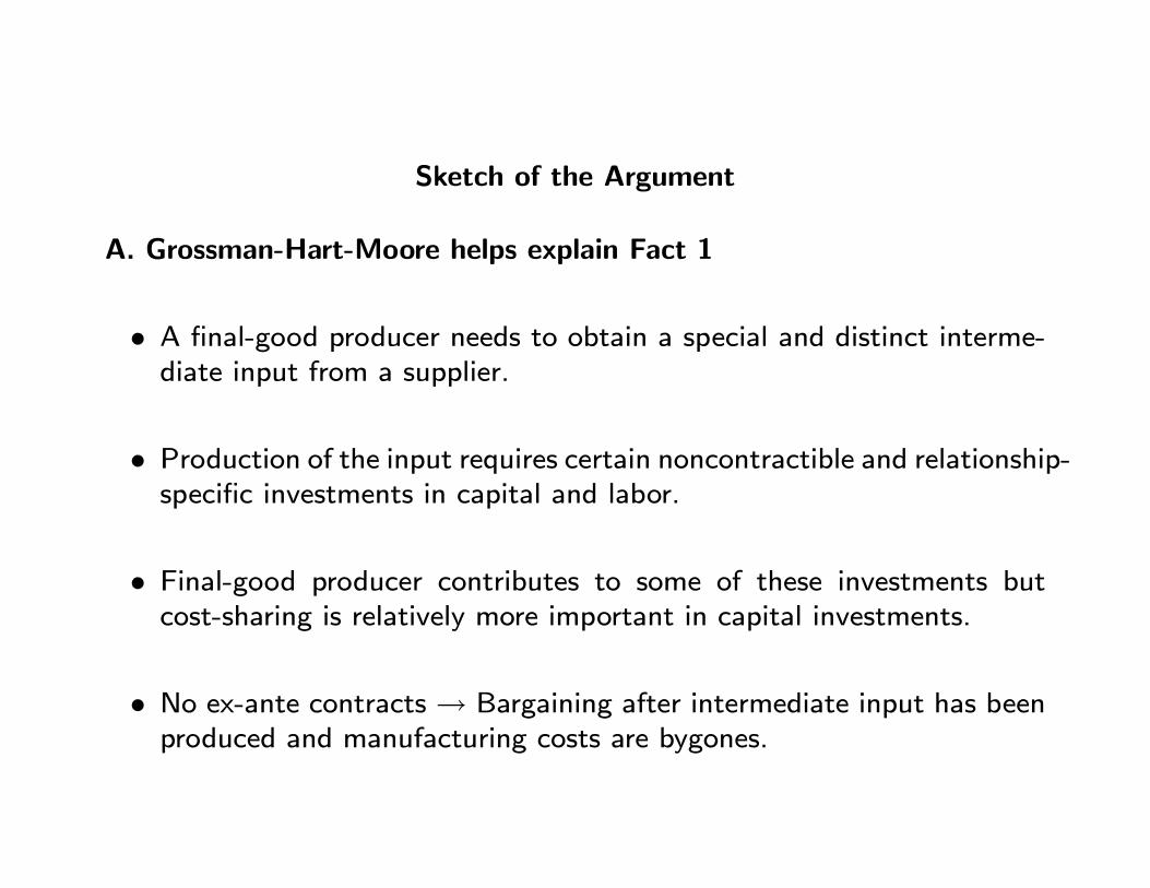
A. Grossman-Hart-Moore helps explain Fact 1

• A final-good producer needs to obtain a special and distinct interme-diate input from a supplier.

• Production of the input requires certain noncontractible and relationship-specific investments in capital and labor.

• Final-good producer contributes to some of these investments butcost-sharing is relatively more important in capital investments.

• No ex-ante contracts → Bargaining after intermediate input has beenproduced and manufacturing costs are bygones.

A. Grossman-Hart-Moore helps explain Fact 1 (continued)

• Ex-post bargaining + lock-in → underinvestment in both capital and

labor.

• Two options: vertical integration or outsourcing. Ownership = enti-

tlement of some residual rights of control → outside option for the

final-good is higher under integration than under outsourcing.

• Inefficiency in labor investments is shown to be relatively higher underintegration than under outsourcing; conversely for capital.

• Ex-ante: choose outsourcing only when the investment in labor isrelatively important in production → close to Fact 1.

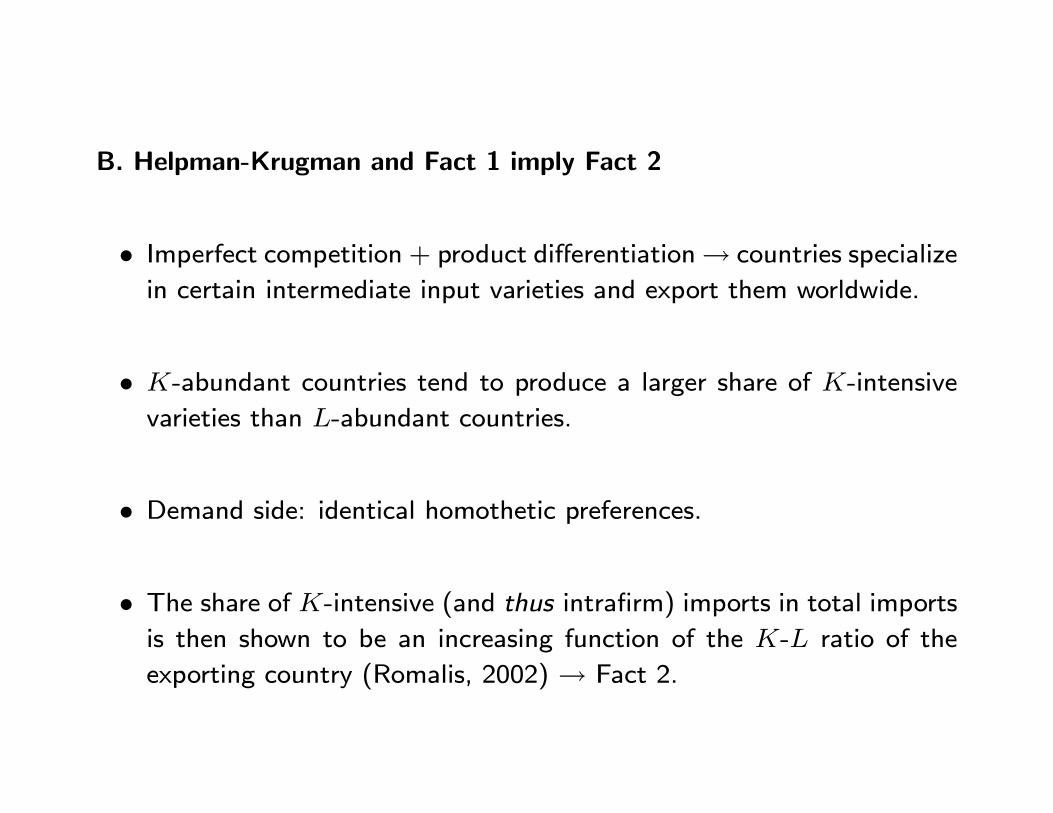
B. Helpman-Krugman and Fact 1 imply Fact 2

• Imperfect competition + product differentiation→ countries specialize

in certain intermediate input varieties and export them worldwide.

• -abundant countries tend to produce a larger share of -intensive

varieties than -abundant countries.

• Demand side: identical homothetic preferences.

• The share of -intensive (and thus intrafirm) imports in total importsis then shown to be an increasing function of the - ratio of the

exporting country (Romalis, 2002) → Fact 2.

Empirical Support

• Business practices suggest that cost-sharing is more common in capitalexpenditures than in labor expenditures.

— Dunning (1993) - MNE with subcontractors - provision of machin-ery and specialized tools, prefinancing of machinery, procurement

assistance in obtaining capital equipment, labor training.

— Milgrom and Roberts (1993) - GM paid for firm- or product-specific

capital equipment needed by the supplier to meet special require-

ments, even though this equipment would be located at the sup-

plier’s facility.

— Aoki (1990) - Japanese firms - close connections with suppliers butconsiderable autonomy in personnel administration.

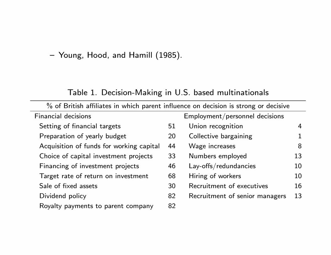
— Young, Hood, and Hamill (1985).

Table 1. Decision-Making in U.S. based multinationals

% of British affiliates in which parent influence on decision is strong or decisive

Financial decisions Employment/personnel decisions

Setting of financial targets 51 Union recognition 4

Preparation of yearly budget 20 Collective bargaining 1

Acquisition of funds for working capital 44 Wage increases 8

Choice of capital investment projects 33 Numbers employed 13

Financing of investment projects 46 Lay-offs/redundancies 10

Target rate of return on investment 68 Hiring of workers 10

Sale of fixed assets 30 Recruitment of executives 16

Dividend policy 82 Recruitment of senior managers 13

Royalty payments to parent company 82

Broad Road Map

• Related Literature

• Set-up of the Model.

• Sketch of Solution and Main Results.

• Econometric Evidence.

• Conclusions.

Related Literature

• General Equilibrium Models of the Multinational Firm:

— Helpman (1984), Markusen (1984), Brainard (1997), Markusen &

Venables (1998) - common failure to model internalization.

— Ethier (1986), Ethier-Markusen (1996) study internalization, but

not its implications for intrafirm trade.

• Incomplete Contracts in General Equilibrium:

— Grossman-Helpman (2002) - closed economy, Williamsonian ap-

proach.

The Closed-Economy Model

• Two-factor (), two-sector () closed economy.

• and are inelastically supplied and freely mobile across sectors.

• In each sector, firms use and to produce a continuum of differ-

entiated varieties.

• Preferences of the representative consumer are of the form:

=µZ

0()

¶µZ

0()

¶1−

with ∈ (0 1).

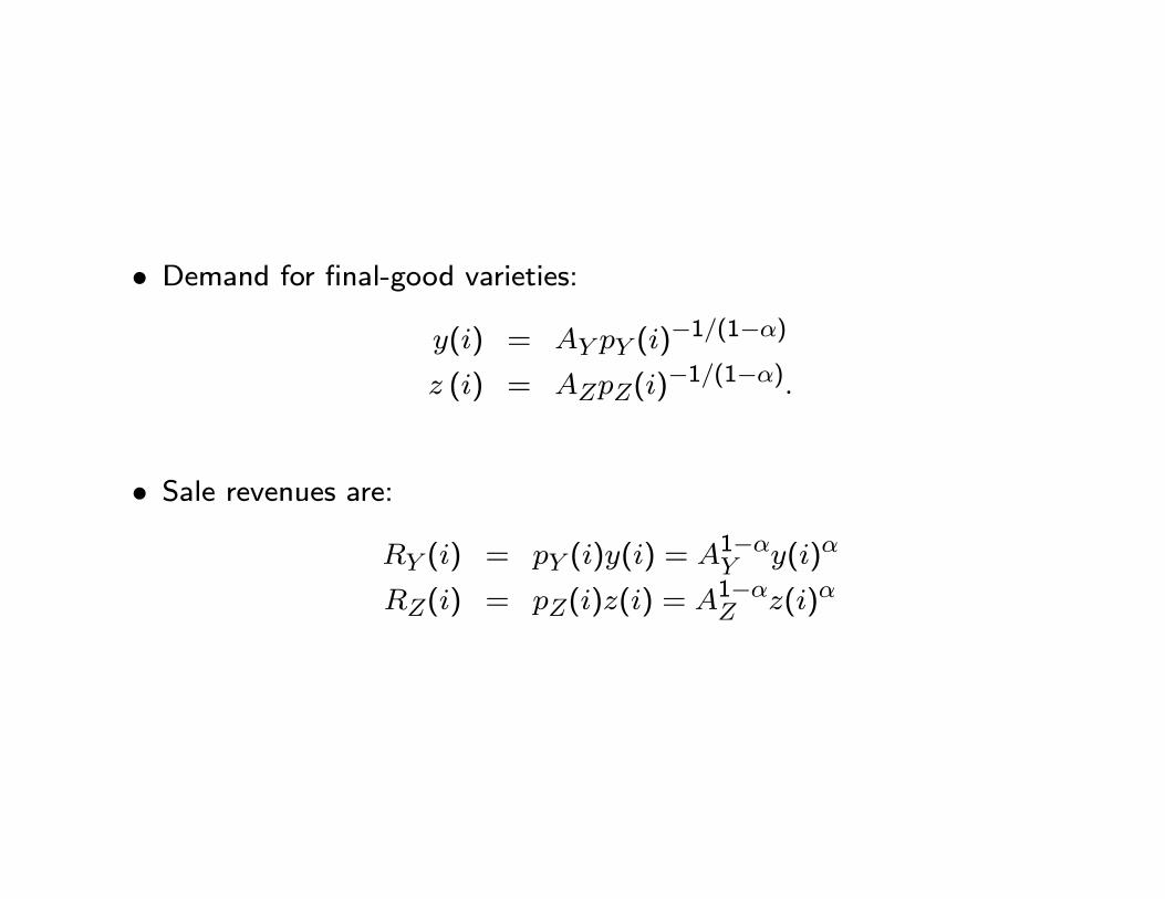
• Demand for final-good varieties:

() = ()−1(1−)

() = ()−1(1−)

• Sale revenues are:

() = ()() = 1− ()

() = ()() = 1− ()

Technology

• Each variety () requires a special and distinct intermediate input

() (() requires ()).

• The input must be of high quality, otherwise output is zero.

• If the input is of high quality, production of the final good requires nofurther costs and () = (), () = ().

Technology (2)

• Production of a high-quality intermediate input requires a combinationof capital () and labor ().

() =

Ã()

! Ã ()

1−

!1−,

for ∈ {}. Let 1 0.

• Low-quality intermediate inputs can be produced at a negligible cost.

• Total fixed costs are 1−, ∈ {}.

Firm structure

• Before any production takes places, decides whether it wants to

enter a given market, and if so, whether to obtain the input from a

vertically-integrated or from a stand-alone .

• Upon entry, makes a lump-sum transfer () to . () is such

that breaks even (ex-ante competitive fringe).

• chooses the mode of organization so as to maximize its ex-ante

profits.

Firm structure (2)

• The labor investment is undertaken by . The capital investment is undertaken by .

• These investments are incurred upon entry and are useless outside therelationship - Williamson’s fundamental transformation.

Contract Incompleteness

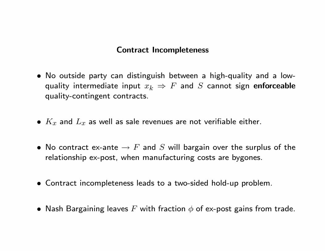
• No outside party can distinguish between a high-quality and a low-quality intermediate input ⇒ and cannot sign enforceablequality-contingent contracts.

• and as well as sale revenues are not verifiable either.

• No contract ex-ante → and will bargain over the surplus of therelationship ex-post, when manufacturing costs are bygones.

• Contract incompleteness leads to a two-sided hold-up problem.

• Nash Bargaining leaves with fraction of ex-post gains from trade.

Contract Incompleteness (2)

• As in Grossman and Hart (1986), ownership will affect the distributionof ex-post surplus through its effect on each party’s outside option.

• Input is completely specific to → outside option for is zero re-

gardless of ownership structure.

• If is a stand-alone firm → ’s outside option is also zero.

• By integrating , obtains the residual rights over a fraction ∈(0 1) of the amount of () produced, which translate into sale rev-

enues of ().

Payoffs in the Nash Bargaining

Final-good producer SupplierNon-Integration () (1− )()

Integration ()³1−

´()

where

= + (1− )

• and are set non-cooperatively to maximize these payoffs. Trade-

off: → 1− 1− .

[FIGURE 3 HERE]

Sketch of the Solution

1. Firm Behavior for a Given Demand

2. Factor Intensity and the Equilibrium Mode of Organization.

3. Industry Equilibrium.

4. General Equilibrium of the Integrated Economy.

5. Split the world endowment of and between ≥ 2 countries andstudy pattern of production and trade.

Firm Behavior for a Given Demand

The Program

maxe∈{} ³

³e´ ³e´´

³e´ = argmax

e

³

³e´´−

³e´ = argmax

³1− e´

³

³e´ ´−

Integrated pairs

• Combining the FOCs of the two constraints with e = yields optimal

, → → and .

• Transfer is chosen s.t. = 0.

• ’s profits are then

=³1− (1− ) + (1− 2 )

´ ×

×

⎛⎜⎝ 1−

³1−

´1−⎞⎟⎠−1−

− 1−

Stand-alone pairs

• Analogous with replacing throughout.

• Find

= (1− (1− ) + (1− 2 )) ×

×Ã

1−

(1− )1−

! −1−

− 1−

Comparison with Complete Contracts

• Compare to case in which the two parties could contract ex-ante andagree on maximizing the value of the relationship, given by

− −

• Incomplete contracts leads to underinvestment in and . Under-

investment in is relatively more severe under integration. Underin-

vestment in is relatively more severe under outsourcing (see Figure

4).

[FIGURE 4 HERE]

Factor Intensity and Ownership Structure

• Let Θ( ) ≡ be profits under integration relative to out-

sourcing.

Proposition 1 There exists a unique b ∈ (0 1) such that Θ(b) = 1.

Furthermore, for all b, Θ() 1 and for all b, Θ() 1.

• All firms with capital intensity below (above) a certain threshold bchoose to outsource (vertically-integrate) production of the interme-

diate input.

Factor Intensity and Ownership Structure (2)

• Getting closer to Fact 1.

• Cobb-Douglas assumption makes Θ () independent of factor prices.Block-recursiveness.

• Other Comparative Statics: Θ(·) 0.

Why is providing ?

• Otherwise, would choose and to

max (1− ) − −

Lemma 1 If 12, final-good producers will always decide to

provide the capital required for production.

• Key Point: the supplier is never given full control. There is an un-modelled non-contractible and inalienable investment by that is in-

dispensable for sale revenues to be positive→ No forward integration.

Empirical Support

• Business practices suggest that cost-sharing is more common in capitalexpenditures than in labor expenditures.

— Dunning (1993) - MNE with subcontractors - provision of machin-ery and specialized tools, prefinancing of machinery, procurement

assistance in obtaining capital equipment, labor training.

— Milgrom and Roberts (1993) - GM paid for firm- or product-specific

capital equipment needed by the supplier to meet special require-

ments, even though this equipment would be located at the sup-

plier’s facility.

— Aoki (1990) - Japanese firms - close connections with suppliers butconsiderable autonomy in personnel administration.

— Young, Hood, and Hamill (1985).

Table 1. Decision-Making in U.S. based multinationals

% of British affiliates in which parent influence on decision is strong or decisive

Financial decisions Employment/personnel decisions

Setting of financial targets 51 Union recognition 4

Preparation of yearly budget 20 Collective bargaining 1

Acquisition of funds for working capital 44 Wage increases 8

Choice of capital investment projects 33 Numbers employed 13

Financing of investment projects 46 Lay-offs/redundancies 10

Target rate of return on investment 68 Hiring of workers 10

Sale of fixed assets 30 Recruitment of executives 16

Dividend policy 82 Recruitment of senior managers 13

Royalty payments to parent company 82

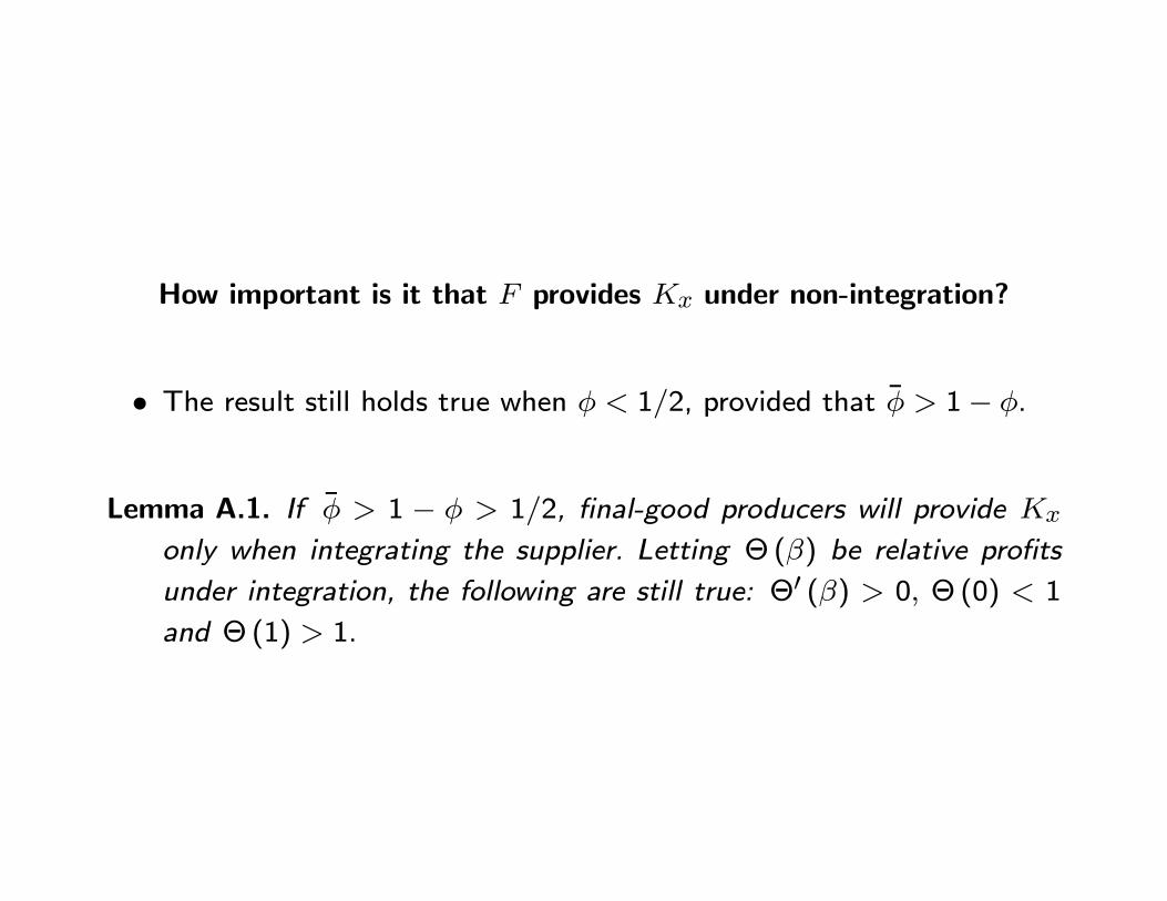
How important is it that provides under non-integration?

• The result still holds true when 12, provided that 1− .

Lemma A.1. If 1 − 12, final-good producers will provide

only when integrating the supplier. Letting Θ () be relative profits

under integration, the following are still true: Θ0 () 0 Θ (0) 1

and Θ (1) 1.

The Program under Partial Contractibility

• Let = , where is contractible, and let ( ) = .

maxe∈{} ³

³e´ ³e´´

³e´ = argmax

e

³

³e´´−

³e´ = argmax

³1− e´

³

³e´ ´−

•

³e´ and ³e´ are independent of . Get same solution.• Key: marginal cost of is increasing in . Setting in advance doesnot solve hold-up.

Industry Equilibrium (Y industry)

• In equilibrium, free entry implies that no firm makes positive profits;

will adjust to ensure = 0.

• Three potential equilibrium modes of organization in industry .

Lemma 3 A mixed equilibrium in industry only exists in a knife-edge

case, namely when =b. An equilibrium with pervasive integration

in industry exists only if b. An equilibrium with pervasive

outsourcing in industry exists only if b.

General Equilibrium

Assumption 2: b .

• In the GE of the integrated economy, income equals spending,

= +

and the product, capital and labor markets clear:X∈{}

³ +

´=

X∈{}

³ +

´=

General Equilibrium (2)

• Equilibrium wage-rental is given by

=

1−

=

(1−g ) + (1− )(1−g)g + (1− )g

,

where the effective capital shares are:

g = ³1 + (1− ) (2− 1)

´g = (1 + (1− )(2− 1))

Note that g g, i.e., contract incompleteness does not createFIR.

• If 12, g and g =⇒ is depressed relative to

complete-contracting world.

The Multi-Country Model

• Now suppose the world is divided in ≥ 2 countries, with country receiving an endowment

³

´.

• Assume that preferences are identical in all countries.

• Factors of production are internationally immobile.

• Assume that for all ∈ , is not “too different” from (sufficient conditions below) → FPE → Integrated Equilibrium.

• Intermediate inputs can be traded at zero cost. Final goods are non-tradable ⇒ each has costless plants.

Pattern of Production

• The factor market clearing conditions in country ∈ are now:X∈{}

³ +

´=

X∈{}

³ +

´=

• FPE ⇒ Differences in production patterns are channelled through and .

• (Hecksher-Ohlin Theorem) If country is relatively capital-abundant

(i.e. ), then and

, where is

’s share in world income, i.e

= +

+

• For the above allocation to be consistent with FPE, we require 0

and 0, or equivalently:

Assumption 3:f ³

1−f ´(1−)

f³1−f´(1−) for all ∈ .

[FIGURE 5 HERE]

Pattern of Trade

• All world trade is in intermediate inputs and .

• A given country ∈ will host + producers of final-goodvarieties.

— a measure will be importing from their integrated suppliers inevery country 6= ;

— a measure will be importing from their independent suppliersin every country 6= .

• Each of these final-good producers in will import a fraction ofworld output of the corresponding variety.

• Average cost transfer pricing → = and = .

• Volume of imports from is

= ³ +

´= ( +)

• Intrafirm imports from are:

− =

• Hence, the share is simply:

− =

µ³1−g´ (1− )

−g

¶³g −g´µ(1− )

+

¶

Main Predictions

• Let = .

Lemma 3 The volume − of U.S. intrafirm imports from country

is an increasing function of the capital-labor ratio and the size

of the exporting country.

Proposition 2 The share − of intrafirm imports in total U.S. imports

from country is an increasing function of the capital-labor ratio

of the exporting country and is independent of its size .

[FIGURE 6 HERE]

[FIGURE 7 HERE]

Econometric Evidence

Specification

1. ln³−

´= 1 + 2 ln () + 0

3 + . Expect 2 0

2. ln³−

´= 1 + 2 ln

³

´+ 3 ln

³´+ 0

4 + . Expect

2 = (1− )³1− −g´ ' 12 and 3 = 0.

3. ln³

−

´= 1+2 ln

³

´+3 ln

³´+ 0

4+. Expect

2 = (1− )³1−g´ ³1− −g´ ' 155 and 3 = 1.

Data: LHS Variables

• Intrafirm U.S. imports are from BEA and comprise:

1. imports shipped by overseas MOFA to their U.S. parents.

2. imports shipped to M.O. U.S. affiliates by their foreign parent.

• Panel of 23 industries and 4 (benchmark) years: 1987, 1989, 1992,and 1994.

• Cross-section of 28 countries for 1992.

• Total U.S. imports are from Feenstra.

Table 2. Share of Intrafirm Imports in total U.S. Imports (%)

by Industry (avg. 1987-94) by Country (1992)

DRU 65.5 FOO 13.9 CHE 64.1 ESP 15.5

OCH 40.9 PAP 12.7 SGP 55.4 AUS 15.5

VEH 39.8 FME 12.6 IRL 53.7 JPN 14.2

ELE 37.3 STO 11.8 CAN 45.1 ISR 12.4

COM 36.7 INS 11.1 NDL 42.2 HKG 11.2

CHE 35.9 TRA 10.7 MEX 41.7 PHL 8.4

CLE 35.7 PLA 9.1 PAN 35.8 ITA 8.1

RUB 23.9 PRI 6.1 GBR 33.2 ARG 5.1

AUD 23.8 LUM 4.1 DEU 31.9 COL 4.6

OEL 18.9 OMA 2.6 MYS 30.1 OAN 4.6

IMA 17.3 TEX 2.3 BEL 27.3 VEN 1.4

BEV 15.1 BRA 25.9 CHL 1.3

FRA 21.6 IDN 1.3

SWE 16.8 EGY 0.1

Data: RHS Variables

• ln(), ln() and ln( ) from NBER-Manufacturing

• ln(&) and ln() from FTC line-of-business

• ln (), ln (), ln () and from Hall and Jones

(1999)

• and from World Development Report (1992).

• from Price Waterhouse.

Table 3. Descriptive Statistics

Obs Mean St. dev. Min Max

ln³−

´

92 -1.90 0.92 -4.74 -0.19

ln() 92 4.26 0.57 3.21 5.73

ln() 92 -0.69 0.60 -1.78 0.60

ln(&) 92 -4.20 1.00 -6.07 -2.47

ln() 92 -4.27 1.10 -6.63 -2.24

ln() 92 1.63 0.92 0.06 3.48

ln( ) 92 -0.66 0.18 -1.13 -0.32

ln³−

´28 -2.08 1.44 -6.67 -0.45

ln () 28 10.54 0.86 8.13 11.59

ln () 28 16.03 1.20 13.63 18.16

ln () 28 0.82 0.19 0.47 1.10

28 0.32 0.08 0.15 0.44

28 6.36 1.22 4.19 8.24

26 7.83 1.23 4.73 9.57

26 6.70 1.22 3.52 8.67

ln³

−

´28 6.36 2.64 -1.39 10.49

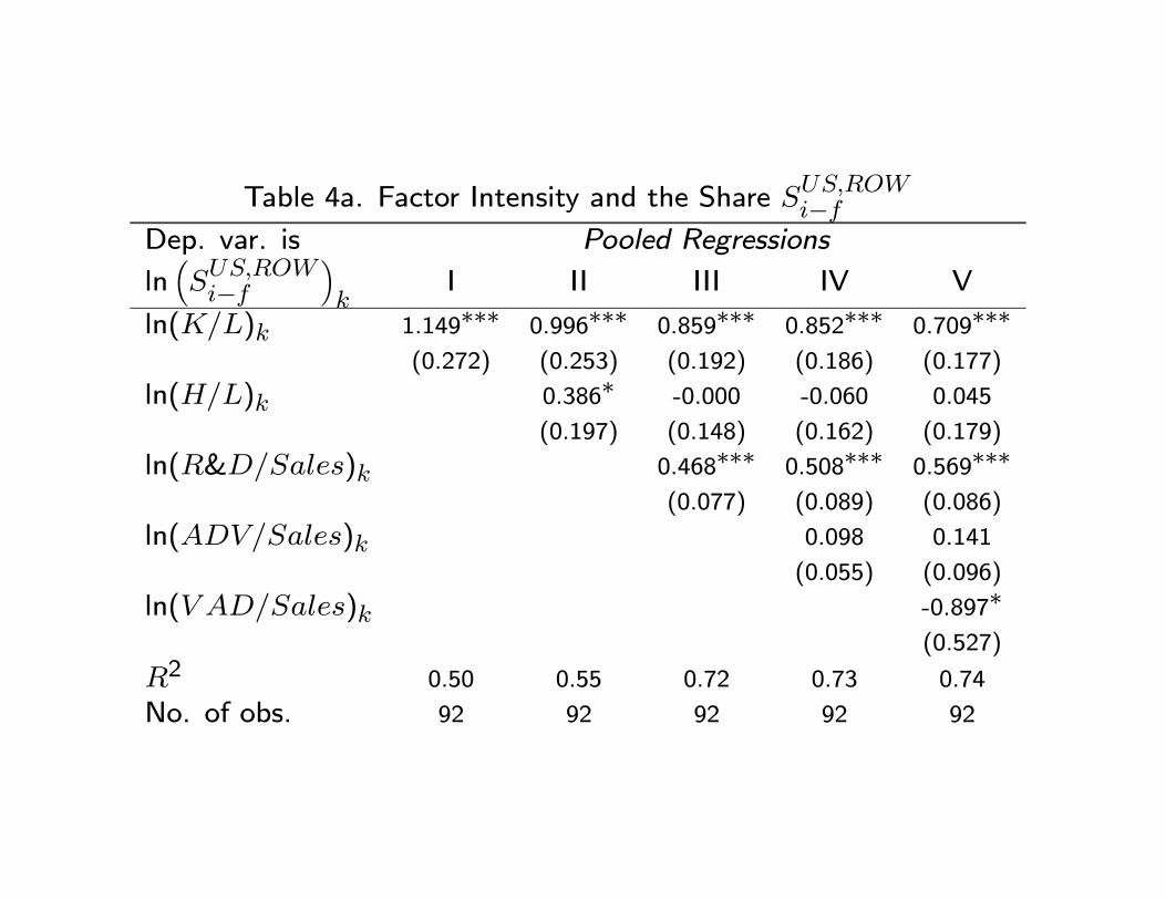
Table 4a. Factor Intensity and the Share −Dep. var. is Pooled Regressions

ln³−

´

I II III IV V

ln() 1.149∗∗∗ 0.996∗∗∗ 0.859∗∗∗ 0.852∗∗∗ 0.709∗∗∗

(0.272) (0.253) (0.192) (0.186) (0.177)

ln() 0.386∗ -0.000 -0.060 0.045

(0.197) (0.148) (0.162) (0.179)

ln(&) 0.468∗∗∗ 0.508∗∗∗ 0.569∗∗∗

(0.077) (0.089) (0.086)

ln() 0.098 0.141

(0.055) (0.096)

ln( ) -0.897∗

(0.527)

2 0.50 0.55 0.72 0.73 0.74

No. of obs. 92 92 92 92 92

Table 4b. Factor Intensity and the Share −Dep. var. is Random Effects Regressions

ln³−

´

I II III IV V

ln() 0.947∗∗∗ 0.861∗∗∗ 0.796∗∗∗ 0.789∗∗∗ 0.804∗∗∗

(0.187) (0.190) (0.160) (0.161) (0.184)

ln() 0.369 -0.015 -0.078 -0.089

(0.213) (0.191) (0.204) (0.214)

ln(&) 0.485∗∗∗ 0.528∗∗∗ 0.520∗∗∗

(0.117) (0.127) (0.135)

ln() 0.088 0.080

(0.096) (0.105)

ln( ) 0.103

(0.622)

2 0.50 0.55 0.72 0.73 0.73

No. of obs. 92 92 92 92 92

Table 5. Factor Endowments and the Share −Dep. var. is

ln³−

´I II III IV V

ln () 1.141∗∗∗ 1.110∗∗∗ 1.244∗∗∗ 1.049∗∗∗ 1.119∗∗

(0.289) (0.299) (0.427) (0.368) (0.399)

ln () -0.133 -0.159 -0.090 0.017

(0.168) (0.164) (0.177) (0.220)

ln () -1.024 -0.374 -0.822

(1.647) (1.584) (1.389)

-0.202 -0.384∗

(0.156) (0.218)

0.292

(0.273)

1.856

(2.932)

2 0.46 0.47 0.48 0.36 0.43

No. of obs. 28 28 28 26 26

Table 6. Factor Endowments and the volume −

Dep. var. is

ln³

−

´I II III IV V

ln () 2.048∗∗∗ 2.192∗∗∗ 2.188∗∗∗ 1.841∗∗∗ 2.096∗∗∗

(0.480) (0.458) (0.716) (0.623) (0.695)

ln () 0.607∗∗ 0.608∗∗ 0.435 0.700

(0.229) (0.268) (0.332) (0.419)

ln () 0.031 0.892 0.708

(3.289) (3.147) (3.052)

-0.624∗∗ -1.006∗∗

(0.259) (0.474)

0.674

(0.560)

-0.647(5.295)

2 0.44 0.52 0.52 0.42 0.49

No. of obs. 28 28 28 26 26

Conclusions

What I did:

• I unveiled two systematic patterns in the intrafirm component of in-ternational trade.

• Traditional trade theory is silent on the boundaries of firms. The theoryof the firm has mostly been partial-equilibrium in scope and has ignoredthe international dimensions of certain intrafirm transactions.

• Building on two workhorse models in international trade and the theoryof the firm, I have constructed a model that, by determining both thepattern of international trade and the boundaries of firms in a unifiedframework, predicts these systematic patterns.

What next?

• Antras (2002)

— Dynamic, Ricardian model of North-South trade in which incom-plete contracting leads to endogenous product cycles as well asendogenous organizational cycles.

— New product cycle: manufacturing shifted to the South first withinfirm boundaries, and only later to independent firms in the South.

• Antras and Helpman (2003)

— Interaction of industry-wide determinants of integration with firm-level heterogeneity → richer patterns of organizational structureboth across and within industries.

Figure 1: Share of Intrafirm U.S. Imports and Relative Factor Intensities

log

of (M

if / M

)

log of (Capital / Employment)3 4 5 6

-4.5

-3

-1.5

0

aud

bev

checlecom

dru

ele

fme foo

ima

ins

lum

och

oel

oma

pap

pla

pri

rub

sto

tex

tra

veh

Notes: The Y-axis corresponds to the logarithm of the share of intrafirm imports in total U.S. imports for 23 manufacturing industries averaged over 4 years: 1987, 1989, 1992, 1994. The X-axis measures the average log of that industry’s ratio of capital stock to total employment, using U.S. data. See Table A.1. for industry codes and Appendix A.4. for data sources.

y = -6.86 + 1.17 x(1.02) (0.24)

R2 = 0.54

Figure 2: Share of Intrafirm Imports and Relative Factor Endowments

Notes: The Y-axis corresponds to the logarithm of the share of intrafirm imports in total U.S. imports for 28 exporting countries in 1992. The X-axis measures the log of the exporting country’s physical capital stock divided by its total number of workers. See Table A.2. for country codes and Appendix A.4. for details on data sources.

log

of (M

if / M

)

log of Capital-Labor Ratio7.5 9 10.5 12

-6

-4

-2

0

ARG

AUS

BELBRA

CAN

CHE

CHL

COL

DEU

EGY

ESP

FRA

GBR

HKG

IDN

IRL

ISR

ITA

JPN

MEXMYS

NDL

OAN

PAN

PHL

SGP

SWE

VEN

y = -14.11 + 1.14 x(2.55) (0.29)

R2 = 0.46

Figure 3: Timing of Events

t0

Choice of ownershipEx-ante transfer T

Fixed costs

t2

Generalized Nash bargaining

t3

Final good produced and

sold

t1

Investments Kx and Lxand intermediate x produced

Figure 4: Complete vs. Incomplete Contracts

Lx

Kx

FV

S *

Kx*

Kx,V

Lx*

F *SV SO

FO

Lx,V Lx,O

Kx,O

A

B

C

Figure 5: Pattern of Production for = 2

ON

OS

LN

KN

KS

LS

w/r B’

E

Y

Z

C

B

nYN

nYS

nZN

nZS

Figure 6: Volume of Intrafirm Imports

OS

KN

KS

LS

w/r B’

EY

Z

C

B

LNON

Figure 7: Share of Intrafirm Imports

ON

OS

LN

KS

LS

w/r B’

B

Y

Z

C

E

KN