first steps in tropical geometry - math.uni-frankfurt.detheobald/publications/tropical.pdf ·...

Contemporary Mathematics

First Steps in Tropical Geometry

Jurgen Richter-Gebert, Bernd Sturmfels, and Thorsten Theobald

Abstract. Tropical algebraic geometry is the geometry of the tropical semi-ring (

�, min, +). Its objects are polyhedral cell complexes which behave like

complex algebraic varieties. We give an introduction to this theory, with anemphasis on plane curves and linear spaces. New results include a completedescription of the families of quadrics through four points in the tropical projec-tive plane and a counterexample to the incidence version of Pappus’ Theorem.

1. Introduction

Idempotent semirings arise in a variety of contexts in applied mathematics,including control theory, optimization and mathematical physics ([2, 3, 9]). Animportant such semiring is the min-plus algebra or tropical semiring (R,⊕,�). Theunderlying set R is the set of real numbers, sometimes augmented by +∞. Thearithmetic operations of tropical addition ⊕ and tropical multiplication � are

x ⊕ y := min{x, y} and a � b := a + b.

The tropical semiring is idempotent in the sense that a ⊕ a ⊕ · · · ⊕ a = a. Whilelinear algebra and matrix theory over idempotent semirings are well-developed andhave had numerous successes in applications, the corresponding analytic geometryhas received less attention until quite recently (see [3] and the references therein).

The n-dimensional real vector space Rn is a module over the tropical semiring(R,⊕,�), with the operations of coordinatewise tropical addition

(a1, . . . , an) ⊕ (b1, . . . , bn) =(

min{a1, b1}, . . . , min{an, bn})

.

and tropical scalar multiplication (which is “scalar addition” classically).

λ � (a1, a2, . . . , an) =(

λ + a1, λ + a2, . . . , λ + an

)

.

Here are two suggestions of how one might define a tropical linear space.

Suggestion 1. A tropical linear space L is a subset of Rn which consists of allsolutions (x1, x2, . . . , xn) to a finite system of tropical linear equations

a1 � x1 ⊕ · · · ⊕ an � xn = b1 � x1 ⊕ · · · ⊕ bn � xn.

Bernd Sturmfels was partially supported by NSF grant DMS-0200729 and a John-von-Neumann Professorship during the summer semester 2003 at Technische Universitat Munchen.2000 Mathematics Subject Classification 14A25, 15A03, 16Y60, 52B70, 68W30.

c©0000 (copyright holder)

1

2 JURGEN RICHTER-GEBERT, BERND STURMFELS, AND THORSTEN THEOBALD

Suggestion 2. A tropical linear space L in Rn consists of all tropical linearcombinations λ�a ⊕ µ� b ⊕ · · · ⊕ ν� c of a fixed finite subset {a, b, . . . , c} ⊂ Rn.

In both cases, the set L is closed under tropical scalar multiplication, L =L + R(1, 1, . . . , 1). We therefore identify L with its image in the tropical projectivespace

TPn−1 = Rn/R(1, 1, . . . , 1).

Let us consider the case of lines in the tropical projective plane (n = 3). Accordingto Suggestion 1, a line in TP

2 would be the solution set of one linear equation

a � x ⊕ b � y ⊕ c � z = a′ � x ⊕ b′ � y ⊕ c′ � z.

Figure 1 shows that such lines are one-dimensional in most cases, but can be two-dimensional. There is a total of twelve combinatorial types; see [3, Figure 5].

O

N

P O

N

P

x = 2 � x ⊕ 1 � y ⊕ 4 � z x = x ⊕ 1 � y ⊕ 4 � z

Figure 1. Two lines according to Suggestion 1. In all our picturesof the tropical projective plane TP

2 we normalize with z = 0.

Suggestion 2 implies that a line in TP2 is the span of two points a and b. This

is the set of the following points in TP2 as the scalars λ and µ range over R:

λ�a⊕µ� b =(

min{λ+a1, µ+ b1}, min{λ+a2, µ+ b2}, min{λ+a3, µ+ b3})

.

Such “lines” are pairs of segments connecting the two points a and b. See Figure 2.

O

N

Pa

b

O

N

P

a

b

O

N

P

a

b

Figure 2. The three combinatorial types of lines in Suggestion 2.

As shown in Figure 3, the span of three points a, b and c in TP2 is usually atwo-dimensional figure. Such figures are called tropical triangles.

FIRST STEPS IN TROPICAL GEOMETRY 3

O

N

P

a

b

c

O

N

P

a

b

c

O

N

P a

b

c

Figure 3. Different combinatorial types of the span of three points.

It is our opinion that both of the suggested definitions of linear spaces are in-correct. Suggestion 2 gives lines that are too small. They are just tropical segmentsas in Figure 2. Also if we attempt to get the entire plane TP2 by the construction inSuggestion 2, then we end up only with tropical triangles as in Figure 3. The linesarising from Suggestion 1 are bigger, but they are sometimes too big. Certainly, noline should be two-dimensional. We wish to argue that both suggestions, in spiteof their algebraic appeal, are not satisfactory for geometry. What we want is this:

Requirement. Lines are one-dimensional objects. Two general lines in the planeshould meet in one point. Two general points in the plane should lie on one line.

Our third and final definition of tropical linear space, to be presented in thenext section, will meet this requirement. We hope that the reader will agree thatthe resulting figures are not too big and not too small but just right.

This paper is organized as follows. In Section 2 we present the general definitionof tropical algebraic varieties. In Section 3 we explain how certain tropical varieties,such as curves in the plane, can be constructed by elementary polyhedral means.Bezout’s Theorem is discussed in Section 4. In Section 5 we study linear systems ofequations in tropical geometry. The tropical Cramer’s rule is shown to compute thestable solutions of these systems. We apply this to construct the unique tropicalconic through any five given points in the plane TP

2. In Section 6, we constructthe pencil of conics through any four points. We show that of the 105 trivalenttrees with six nodes representing such lines [15, §3] precisely 14 trees arise from

quadruples of points in TP2. Section 7 addresses the validity of incidence theorems

in tropical geometry. We show that Pappus’ Theorem is false in general, but weconjecture that a certain constructive version of Pappus’ Theorem is valid. We alsoreport on first steps in implementing tropical geometry in the software Cinderella[11].

Tropical algebraic geometry is an emerging field of mathematics, and differentresearchers have used different names for tropical varieties: logarithmic limit sets,Bergman fans, Bieri-Groves sets, and non-archimedean amoebas. All of these no-tions are essentially the same. Recent references include [5, 6, 7, 14, 17, 19]. Forthe relationship to Maslov dequantization see [20].

2. Algebraic definition of tropical varieties

In our algebraic definition of tropical varieties, we start from a lifting to thefield of algebraic functions in one variable. Similar liftings have already been used


in the max-plus literature in the context of Cramer’s rule and eigenvalue problems(see [8, 13]). Our own version of Cramer’s rule will be given in Section 5.

The order of a rational function in one complex variable t is the order of its zeroor pole at the origin. It is computed as the smallest exponent in the numeratorpolynomial minus the smallest exponent in the denominator polynomial. Thisdefinition of order extends uniquely to the algebraic closure K = C(t) of the fieldC(t) of rational functions. Namely, any non-zero algebraic function p(t) ∈ K canbe locally expressed as a Puiseux series

p(t) = c1tq1 + c2t

q2 + c3tq3 + · · · .

Here c1, c2, . . . are non-zero complex numbers and q1 < q2 < · · · are rational num-bers with bounded denominators. The order of p(t) is the exponent q1. The orderof an n-tuple of algebraic functions is the n-tuple of their orders. This gives a map

(1) order : (K\{0})n → Qn ⊂ Rn.

Let I be any ideal in the Laurent polynomial ring K[x±11 , . . . , x±1

n ] and consider itsaffine variety V (I) ⊂ (K\{0})n over the algebraically closed field K. The imageof V (I) under the map (1) is a subset of Qn. We take its topological closure. Theresulting subset of Rn is the tropical variety T (I).

Definition 2.1. A tropical algebraic variety is any subset of Rn of the form

T (I) = order(V (I)),

where I is an ideal in the ring of Laurent polynomials in n unknowns with coeffi-cients in the field K of algebraic functions in one complex variable t.

An ideal I ⊂ K[x±11 , . . . , x±1

n ] is homogeneous if all monomials xi11 · · ·xin

n ap-pearing in a given generator of I have the same total degree i1 + · · · + in. Sucha homogeneous ideal I defines a variety V (I) in projective space Pn−1

K minus thecoordinate hyperplanes xi = 0. Its image under the order map (1) becomes a subsetof tropical projective space TP

n−1 = Rn/R(1, 1, . . . , 1).

Definition 2.2. A tropical projective variety is a subset of TPn−1 of the form

T (I) = order(V (I))/R(1, 1, . . . , 1)

where I is a homogeneous ideal in the Laurent polynomial ring K[x±11 , . . . , x±1

n ].

We are now prepared to give the correct definition of tropical linear space.

Definition 2.3. A tropical linear space is a subset of tropical projective spaceTP

n−1 of the form T (I) where the ideal I is generated by linear forms

p1(t) · x1 + p2(t) · x2 + · · · + pn(t) · xn

whose coefficients pi(t) are algebraic functions in one complex variable t.

Before discussing the geometry of tropical varieties in general, let us first seethat this definition satisfies the requirement expressed in the introduction.

Example 2.4. Lines in the tropical plane are defined by principal ideals

I = 〈 p1(t) · x1 + p2(t) · x2 + p3(t) · x3 〉.


O

C

D

EF

G

H

N

P O

C

D

E

N

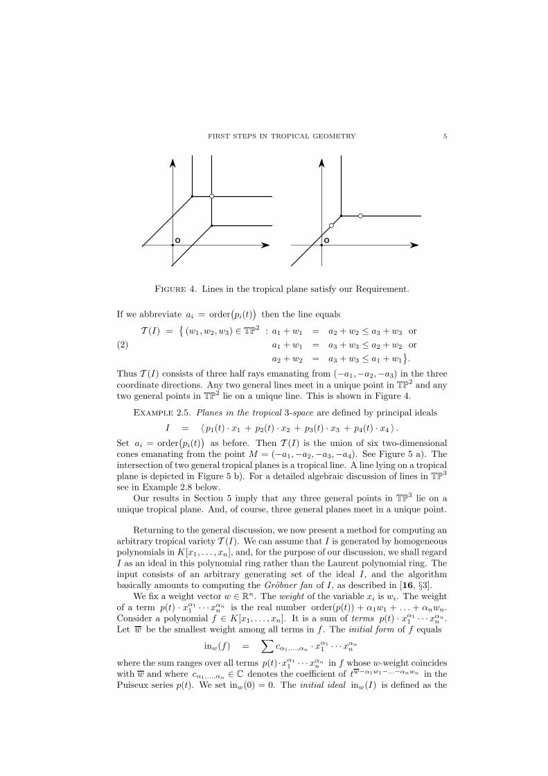
P

Figure 4. Lines in the tropical plane satisfy our Requirement.

If we abbreviate ai = order(

pi(t))

then the line equals

T (I) ={

(w1, w2, w3) ∈ TP2 : a1 + w1 = a2 + w2 ≤ a3 + w3 or

a1 + w1 = a3 + w3 ≤ a2 + w2 or(2)

a2 + w2 = a3 + w3 ≤ a1 + w1

}

.

Thus T (I) consists of three half rays emanating from (−a1,−a2,−a3) in the threecoordinate directions. Any two general lines meet in a unique point in TP

2 and anytwo general points in TP2 lie on a unique line. This is shown in Figure 4.

Example 2.5. Planes in the tropical 3-space are defined by principal ideals

I = 〈 p1(t) · x1 + p2(t) · x2 + p3(t) · x3 + p4(t) · x4 〉 .

Set ai = order(

pi(t))

as before. Then T (I) is the union of six two-dimensionalcones emanating from the point M = (−a1,−a2,−a3,−a4). See Figure 5 a). Theintersection of two general tropical planes is a tropical line. A line lying on a tropicalplane is depicted in Figure 5 b). For a detailed algebraic discussion of lines in TP

3

see in Example 2.8 below.Our results in Section 5 imply that any three general points in TP

3 lie on aunique tropical plane. And, of course, three general planes meet in a unique point.

Returning to the general discussion, we now present a method for computing anarbitrary tropical variety T (I). We can assume that I is generated by homogeneouspolynomials in K[x1, . . . , xn], and, for the purpose of our discussion, we shall regardI as an ideal in this polynomial ring rather than the Laurent polynomial ring. Theinput consists of an arbitrary generating set of the ideal I , and the algorithmbasically amounts to computing the Grobner fan of I , as described in [16, §3].

We fix a weight vector w ∈ Rn. The weight of the variable xi is wi. The weightof a term p(t) · xα1

1 · · ·xαn

n is the real number order(p(t)) + α1w1 + . . . + αnwn.Consider a polynomial f ∈ K[x1, . . . , xn]. It is a sum of terms p(t) · xα1

1 · · ·xαn

n .Let w be the smallest weight among all terms in f . The initial form of f equals

inw(f) =∑

cα1,...,αn· xα1

1 · · ·xαn

n

where the sum ranges over all terms p(t) ·xα11 · · ·xαn

n in f whose w-weight coincideswith w and where cα1,...,αn

∈ C denotes the coefficient of tw−α1w1−...−αnwn in thePuiseux series p(t). We set inw(0) = 0. The initial ideal inw(I) is defined as the


4

3

1

2M

4

3

1

2M

a) b)

Figure 5. A tropical plane and a tropical line in TP3.

ideal generated by all initial forms inw(f) as f runs over I . For a fixed ideal I ,there are only finitely many initial ideals, and they can be computed using thealgorithms in [16, §3]. This implies the following result; see also [17, §9] and [15].

Theorem 2.6. Every ideal I has a finite subset G with the following properties:

(1) If w ∈ T (I) then {inw(g) : g ∈ G}

generates the initial ideal inw(I).

(2) If w 6∈ T (I) then {inw(g) : g ∈ G}

contains a monomial.

The finite set G in this theorem is said to be a tropical basis of the ideal I . IfI is generated by a single polynomial f , then the singleton {f} is a tropical basisof I . If I is generated by linear forms, then the set of all circuits in I is a tropicalbasis of I . These are the linear forms in I whose set of variables is minimal withrespect to inclusion. For any ideal I we have T (I) = ∩g∈GT (〈g〉). We note that anearlier version of this paper made the claim that every universal Grobner basis ofI is automatically a tropical basis, but this claim is not true.

Theorem 2.6 implies that every tropical variety T (I) is a polyhedral cell com-plex, i.e., it is a finite union of closed convex polyhedra in TP

n−1 where the inter-section of any two polyhedra is a common face. Bieri and Groves [1] proved thatthe dimension of this cell complex coincides with the Krull dimension of the ringK[x±1

1 , . . . , x±1n ]/I . An alternative proof using Grobner bases appears in [17, §9].

Theorem 2.7. If V (I) is equidimensional of dimension d then so is T (I).

In order to appreciate the role played by the tropical basis G as the represen-tation of its ideal I , one needs to look at varieties that are not hypersurfaces. Thesimplest example is that of a line in the three-dimensional space TP3.

Example 2.8. A line in three-space is the tropical variety T (I) of an ideal Iwhich is generated by a two-dimensional space of linear forms in K[x1, x2, x3, x4].


A tropical basis of such an ideal I consists of four linear forms,

U ={

p12(t) · x2 + p13(t) · x3 + p14(t) · x4,

−p12(t) · x1 + p23(t) · x3 + p24(t) · x4,

−p13(t) · x1 − p23(t) · x2 + p34(t) · x4,

−p14(t) · x1 − p24(t) · x2 − p34(t) · x3

}

,

where the coefficients of the linear forms satisfy the Grassmann-Plucker relation

(3) p12(t) · p34(t) − p13(t) · p24(t) + p14(t) · p23(t) = 0.

We abbreviate aij = order(

pij(t))

. According to Theorem 2.6, the line T (I) is the

set of all points w ∈ TP3 which satisfy a Boolean combination of linear inequalities:(

a12 + x2 = a13 + x3 ≤ a14 + x4 or

a12 + x2 = a14 + x4 ≤ a13 + x3 or a13 + x3 = a14 + x4 ≤ a12 + x2

)

and(

a12 + x1 = a23 + x3 ≤ a24 + x4 or

a12 + x1 = a24 + x4 ≤ a23 + x3 or a23 + x3 = a24 + x4 ≤ a12 + x1

)

and(

a13 + x1 = a23 + x2 ≤ a34 + x4 or

a13 + x1 = a34 + x4 ≤ a23 + x2 or a23 + x2 = a34 + x4 ≤ a13 + x1

)

and(

a14 + x1 = a24 + x2 ≤ a34 + x3 or

a14 + x1 = a34 + x3 ≤ a24 + x2 or a24 + x2 = a34 + x3 ≤ a14 + x1

)

.

To resolve this Boolean combination, one distinguishes three cases arising from (3):

Case [12, 34] : a14 + a23 = a13 + a24 ≤ a12 + a34,Case [13, 24] : a14 + a23 = a12 + a34 ≤ a13 + a24,Case [14, 23] : a13 + a24 = a12 + a34 ≤ a14 + a23.

In each case, the line T (I) consists of a line segment, with two of the four coordinaterays emanating from each end point. The two end points of the line segment are

Case [12, 34] : (a23 + a34, a13 + a34, a14 + a23, a13 + a23) and(a13 + a24, a13 + a14, a12 + a14, a12 + a13) ,

Case [13, 24] : (a24 + a34, a14 + a34, a14 + a24, a12 + a34) and(a23 + a34, a13 + a34, a12 + a34, a13 + a23) ,

Case [14, 23] : (a23 + a34, a13 + a34, a12 + a34, a13 + a23) and(a24 + a34, a14 + a34, a14 + a24, a12 + a34) .

1

2

3

4

1 2

3 4

1 2

34

Figure 6. The three types of tropical lines in TP3.


The three types of lines in TP3 are depicted in Figure 6. Combinatorially, they

are the trivalent trees with four labeled leaves. It was shown in [15] that lines inTPn−1 correspond to trivalent trees with n labeled leaves. See Example 3.8 below.

3. Polyhedral construction of tropical varieties

After our excursion in the last section to polynomials over the field K, let usnow return to the tropical semiring (R,⊕,�). Our aim is to derive an elementarydescription of tropical varieties. A tropical monomial is an expression of the form

(4) c � xa11 � · · · � xan

n ,

where the powers of the variables are computed tropically as well, for instance,x3

1 = x1�x1�x1. The tropical monomial (4) represents the classical linear function

Rn → R , (x1, . . . , xn) 7→ a1x1 + · · · + anxn + c.

A tropical polynomial is a finite tropical sum of tropical monomials,

(5) F = c1 � xa111 � · · · � xa1n

n ⊕ · · · ⊕ cr � xar11 � · · · � xarn

n .

Remark 3.1. The tropical polynomial F is a piecewise linear concave function,given as the minimum of r linear functions (x1, . . . , xn) 7→ aj1x1 + · · ·+ajnxn +cj.

We define the tropical hypersurface T (F ) as the set of all points x = (x1, . . . , xn)in Rn with the property that F is not linear at x. Equivalently, T (F ) is theset of points x at which the minimum is attained by two or more of the linearfunctions. Figure 7 shows the graph of the piecewise-linear concave function F andthe resulting curve T (F ) ⊂ R2 for a quadratic tropical polynomial F (x, y).

e

d+yf+x

c+2ya+2x b+x+y

Figure 7. The graph of a piecewise linear concave function on R2.

Lemma 3.2. If F is a tropical polynomial then there exists a polynomial f ∈K[x1, . . . , xn] such that T (F ) = T (〈f〉), and vice versa.

Proof. If F is the tropical polynomial (5) then we define

(6) f =

r∑

i=1

pi(t) · xai11 · · ·xain

n ,


where pi(t) ∈ K is any Puiseux series of order ci, for instance, pi(t) = tci . SinceG = {f} is a tropical basis for its ideal, Theorem 2.6 implies T (F ) = T (〈f〉).Conversely, given any polynomial f we can define a tropical polynomial F definingthe same tropical hypersurface in Rn by setting ci = order(pi(t)). �

Theorem 3.3. Every purely (n − 1)-dimensional tropical variety in Rn is atropical hypersurface and hence equals T (F ) for some tropical polynomial F .

Proof. Let X = T (I) be a tropical variety of pure dimension n−1 in Rn. Thismeans that every maximal face of the polyhedral complex is a convex polyhedronof dimension n − 1. If P1, . . . , Ps are the minimal primes of the ideal I then

X = T (P1) ∪ T (P2) ∪ · · · ∪ T (Ps).

Each T (Pi) is pure of codimension 1, hence Theorem 2.7 implies that Pi is a codi-mension 1 prime in the polynomial ring K[x1, . . . , xn]. The prime ideal Pi is gen-erated by a single irreducible polynomial, Pi = 〈fi〉. If we set f = f1f2 · · · fs thenX = T (〈f〉), and Lemma 3.2 gives the desired conclusion. �

Theorem 3.3 states that every tropical hypersurface in Rn has an elementaryconstruction as the locus where a piecewise linear concave function fails to belinear. Tropical hypersurfaces in TP

n−1 arise in the same manner from homogeneoustropical polynomials (5), where ai1+· · ·+ain is the same for all i. We next describethis elementary construction for some curves in TP

2 and some surfaces in TP3.

Example 3.4. Quadratic curves in the plane are defined by tropical quadrics

F = a1�x�x ⊕ a2�x�y ⊕ a3�y�y ⊕ a4�y�z ⊕ a5�z�z ⊕ a6�x�z.

The curve T (F ) is a graph which has six unbounded edges and at most threebounded edges. The unbounded edges are pairs of parallel half rays in the threecoordinate directions. The number of bounded edges depends on the 3 × 3-matrix

(7)

a1 a2 a6

a2 a3 a4

a6 a4 a5

.

We regard the row vectors of this matrix as three points in TP2. If all three pointsare identical then T (F ) is a tropical line counted with multiplicity two. If the threepoints lie on a tropical line then T (F ) is the union of two tropical lines. Here thenumber of bounded edges of T (F ) is two. In the general situation, the three pointsdo not lie on a tropical line. Up to symmetry, there are five such general cases:

Case a: T (F ) looks like a tropical line of multiplicity two (depicted in Figure 8 a)).This happens if and only if

2a2 ≥ a1 + a3 and 2a4 ≥ a3 + a5 and 2a6 ≥ a1 + a5 .

Case b: T (F ) has two double half rays: There are three symmetric possibilities.The one in Figure 8 b) occurs if and only if

2a2 ≥ a1 + a3 and 2a4 ≥ a3 + a5 and 2a6 < a1 + a5 .

Case c: T (F ) has one double half ray: The double half ray is emanating in they-direction if and only if

2a2 < a1 + a3 and 2a4 < a3 + a5 and 2a6 ≥ a1 + a5 .


Figure 8 c) depicts the two combinatorial types for this situation. They are distin-guished by whether 2a2 + a5 − a1 − 2a4 is negative or positive.

a) b) c)

Figure 8. Types of non-proper tropical conics in TP2.

Case d: T (F ) has one vertex not on any half ray. This happens if and only if

a2 + a4 < a3 + a6 and a2 + a6 < a1 + a4 and a4 + a6 < a2 + a5 .

If one of these inequalities becomes an equation, then T (F ) is a union of two lines.

Case e: T (F ) has four vertices and each of them lies on some half ray. Algebraically,

2a2 < a1 + a3 and 2a4 < a3 + a5 and 2a6 < a1 + a5

and (a2 + a4 > a3 + a6 or a2 + a6 > a1 + a4 or a4 + a6 > a2 + a5) .

d) e)

Figure 9. Types of proper tropical conics in TP2.

The curves in cases d) and e) are called proper conics. They are shown in

Figure 9. The set of proper conics forms a polyhedral cone. Its closure in TP5 is

called the cone of proper conics. This cone is defined by the three inequalities

(8) 2a2 ≤ a1 + a3 and 2a4 ≤ a3 + a5 and 2a6 ≤ a1 + a5 .

We will see later that proper conics play a special role in interpolation. �

We next describe arbitrary curves in the tropical plane TP2. Let A be a subsetof {(i, j, k) ∈ N3

0 : i + j + k = d} for some d and consider a tropical polynomial

(9) F (x, y, z) =∑

(i,j,k)∈A

aijk � xi � yj � zk , where aijk ∈ R.

Then T (F ) is a tropical curve in the tropical projective plane TP2, and Theorem 3.3

implies that every tropical curve in TP2 has the form T (F ) for some F .


Here is an algorithm for drawing the curve T (F ) in the plane. The input tothis algorithm is the support A and the list of coefficients aijk . For any pair ofpoints (i′, j′, k′), (i′′, j′′, k′′) ∈ A, consider the system of linear inequalities

ai′j′k′ + i′x + j′y + k′z = ai′′j′′k′′ + i′′x + j′′y + k′′z

≤ aijk + ix + jy + kz for (i, j, k) ∈ A .

The solution set to this system is either empty or a point or a segment or a ray inTP

2. The tropical curve T (F ) is the union of these segments and rays.It appears as if the running time of this procedure is quadratic in the cardinality

of A, as we are considering arbitrary pairs of points (i′, j′, k′) and (i′′, j′′, k′′) in A.However, most of these pairs can be ruled out a priori. The following refinedalgorithm runs in time O(m log m) where m is the cardinality of A. Compute theconvex hull of the points (i, j, k, aijk). This is a three-dimensional polytope. Thelower faces of this polytope project bijectively onto the convex hull of A underdeleting the last coordinate. This defines a regular subdivision ∆ of A. A pair ofvertices (i′, j′, k′) and (i′′, j′′, k′′) needs to be considered if and only if they form anedge in the regular subdivision ∆. The segments of T (F ) arise from the interioredges of ∆, and the rays of T (F ) arise from the boundary edges of ∆. This shows:

Proposition 3.5. The tropical curve T (F ) is an embedded graph in TP2 which

is dual to the regular subdivision ∆ of the support A of the tropical polynomial F .Corresponding edges of T (F ) and ∆ are perpendicular.

If the coefficients of F in (9) are sufficiently generic then the subdivision ∆ isa regular triangulation. This means that the curve T (F ) is a trivalent graph.

Figure 10. Tropical biquadratic curves.

Figure 10 shows two tropical curves whose support is a square with side lengthtwo. In both cases, the corresponding subdivision ∆ is drawn below the curve T (F ).


These are tropical versions of biquadratic curves in P1 × P1, so they representfamilies of elliptic curves over K. The unique cycle in T (F ) arises from the interiorvertex of ∆. The same construction yields tropical Calabi-Yau hypersurfaces in alldimensions.

All the edges in a tropical curve T (F ) have a natural multiplicity, which is thelattice length of the corresponding edge in ∆. In our algorithm, the multiplicityis computed as the greatest common divisor of i′ − i′′, j′ − j′′ and k′ − k′′. Let pbe any vertex of the tropical curve T (F ), let v1, v2, . . . , vr be the primitive latticevectors in the directions of the edges emanating from p, and let m1, m2, . . . , mr bethe multiplicities of these edges. Then the following equilibrium condition holds:

(10) m1 · v1 + m2 · v2 + · · · + mr · vr = 0.

The validity of this identity can be seen by considering the convex r-gon dual to pin the subdivision ∆. The edges of this r-gon are obtained from the vectors mi · vi

by a 90 degree rotation. But, clearly, the edges of a convex polygon sum to zero.Our next theorem states that this equilibrium condition actually characterizes

tropical curves in TP2. This remarkable fact provides an alternative definition oftropical curves. A subset Γ of TP

2 is a rational graph if Γ is a finite union ofrays and segments whose endpoints and directions have coordinates in the rationalnumbers Q, and each ray or segment has a positive integral multiplicity. A rationalgraph Γ is said to be balanced if the condition (10) holds at each vertex p of Γ.

Theorem 3.6. The tropical curves in TP2 are the balanced rational graphs.

Proof. We have shown that every tropical curve is a balanced rational graph.For the converse, suppose that Γ is any rational graph which is balanced. Consider-ing the connected components of Γ separately, we can assume that Γ is connected.By a theorem of Crapo and Whiteley ([4], see also [10, Section 13.1]), the balancedgraph Γ is the projection of the lower edges of a convex polytope. The rationality ofΓ ensures that we can choose this polytope to be rational. Its defining inequalitieshave the form ix+ jy +kz ≥ aijk for some real numbers aijk . Now define a tropicalpolynomial F as in (5). Then our algorithm implies that Γ equals T (F ). Theorem3.3 completes the proof. �

Our polyhedral construction of curves can be generalized to hypersurfaces intropical projective space TP

n−1. This raises the question whether the class of alltropical varieties has a similar characterization. If so, then perhaps the algebraic in-troduction in Section 2 was irrelevant? We wish to argue that this is most certainlynot the case. Here is the crucial definition. A subset of Rn or TP

n−1 is a tropicalprevariety if it is the intersection of finitely many tropical hypersurfaces T (F ).

Lemma 3.7. Every tropical variety is a tropical prevariety, but not conversely.

Proof. By Theorem 2.6 and Theorem 3.3, every tropical variety is a finiteintersection of tropical hypersurfaces, arising from the polynomials in a tropicalbasis. But there are many examples of tropical prevarieties which are not tropicalvarieties. Consider the tropical lines T (L) and T (L′) where

L = 0 � x ⊕ 0 � y ⊕ 0 � z and L′ = 0 � x ⊕ 0 � y ⊕ 1 � z .

Then T (L) ∩ T (L′) is the half ray consisting of all points (a, a, 0) with a ≤ 0.Such a half ray is not a tropical variety. �


When performing constructions in tropical algebraic geometry, it appears to becrucial that we work with tropical varieties and not just with tropical prevarieties.The distinction between these two categories is very subtle, with the algebraicnotion of a tropical basis providing the key. In order for a tropical prevariety tobe a tropical variety, the defining tropical hypersurfaces must obey some strongcombinatorial consistency conditions, namely, those present among the Newtonpolytopes of some polynomials which form a tropical basis.

Synthetic constructions of families of tropical varieties that are not hypersur-faces require great care. The simplest case is that of lines in projective space TP

n−1.

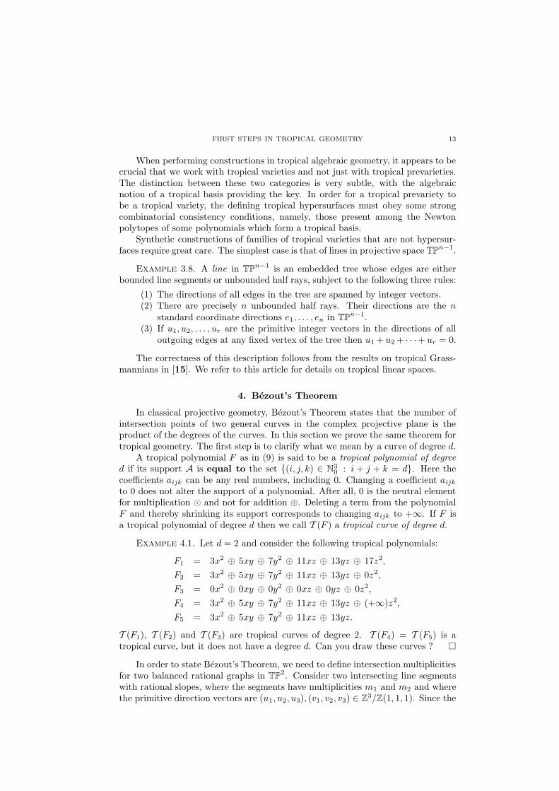
Example 3.8. A line in TPn−1 is an embedded tree whose edges are either

bounded line segments or unbounded half rays, subject to the following three rules:

(1) The directions of all edges in the tree are spanned by integer vectors.(2) There are precisely n unbounded half rays. Their directions are the n

standard coordinate directions e1, . . . , en in TPn−1.(3) If u1, u2, . . . , ur are the primitive integer vectors in the directions of all

outgoing edges at any fixed vertex of the tree then u1 + u2 + · · ·+ ur = 0.

The correctness of this description follows from the results on tropical Grass-mannians in [15]. We refer to this article for details on tropical linear spaces.

4. Bezout’s Theorem

In classical projective geometry, Bezout’s Theorem states that the number ofintersection points of two general curves in the complex projective plane is theproduct of the degrees of the curves. In this section we prove the same theorem fortropical geometry. The first step is to clarify what we mean by a curve of degree d.

A tropical polynomial F as in (9) is said to be a tropical polynomial of degreed if its support A is equal to the set {(i, j, k) ∈ N3

0 : i + j + k = d}. Here thecoefficients aijk can be any real numbers, including 0. Changing a coefficient aijk

to 0 does not alter the support of a polynomial. After all, 0 is the neutral elementfor multiplication � and not for addition ⊕. Deleting a term from the polynomialF and thereby shrinking its support corresponds to changing aijk to +∞. If F isa tropical polynomial of degree d then we call T (F ) a tropical curve of degree d.

Example 4.1. Let d = 2 and consider the following tropical polynomials:

F1 = 3x2 ⊕ 5xy ⊕ 7y2 ⊕ 11xz ⊕ 13yz ⊕ 17z2,

F2 = 3x2 ⊕ 5xy ⊕ 7y2 ⊕ 11xz ⊕ 13yz ⊕ 0z2,

F3 = 0x2 ⊕ 0xy ⊕ 0y2 ⊕ 0xz ⊕ 0yz ⊕ 0z2,

F4 = 3x2 ⊕ 5xy ⊕ 7y2 ⊕ 11xz ⊕ 13yz ⊕ (+∞)z2,

F5 = 3x2 ⊕ 5xy ⊕ 7y2 ⊕ 11xz ⊕ 13yz.

T (F1), T (F2) and T (F3) are tropical curves of degree 2. T (F4) = T (F5) is atropical curve, but it does not have a degree d. Can you draw these curves ? �

In order to state Bezout’s Theorem, we need to define intersection multiplicitiesfor two balanced rational graphs in TP

2. Consider two intersecting line segmentswith rational slopes, where the segments have multiplicities m1 and m2 and wherethe primitive direction vectors are (u1, u2, u3), (v1, v2, v3) ∈ Z3/Z(1, 1, 1). Since the


line segments are not parallel, the following determinant is nonzero:

det

u1 u2 u3

v1 v2 v3

1 1 1

The (tropical) multiplicity of the intersection point is defined as the absolute valueof this determinant times m1 times m2.

Theorem 4.2. Consider two tropical curves C and D of degrees c and d inthe tropical projective plane TP2. If the two curves intersect in finitely many pointsthen the number of intersection points, counting multiplicities, is equal to c · d.

B

AB

A

Figure 11. Non-transversal intersection of a line and a conic.

We say that the curves C and D intersect transversally if each intersection pointlies in the relative interior of an edge of C and in the relative interior of an edgeof D. Theorem 4.2 is now properly stated for the case of transversal intersections.Figure 11 shows a non-transversal intersection of a tropical conic with a tropicalline. In the left picture a slight perturbation of the situation is shown. It showsthat the point of intersection really comes from two points of intersection and hasto be counted with the multiplicity that is the sum of the two points in the nearbysituation. We will first give the proof of Bezout’s Theorem for the transversal case,and subsequently we will discuss the case of non-transversal intersections.

Proof. The statement holds for curves in special position for which all inter-section points occur among the half rays of the first curve in x-direction and thehalf rays of the second curve in y-direction. Such a position is shown in Figure 12.

The following homotopy moves any instance of two transversally intersectingcurves to such a special situation. We fix the first curve C and we translate thesecond curve D with constant velocity along a sufficiently general piecewise linearpath. Let Dt denote the curve D at time t ≥ 0. We can assume that for no valueof t a vertex of C coincides with a vertex of Dt and that for all but finitely manyvalues of t the two curves C and Dt intersect transversally. Suppose these specialvalues of t are the time stamps t1 < t2 < · · · < tr. For any value of t strictlybetween two successive time stamps ti and ti+1, the number of intersection pointsin C ∩ Dt remains unchanged, and so does the multiplicity of each intersectionpoint. We claim that the total intersection number also remains unchanged acrossa time stamp ti.

Let P be the set of branching points of C which are also contained in Dtiand

the set of branching points of Dtiwhich are also contained in C. Since P is finite


Figure 12. Two conics intersect in four points.

it suffices to show the invariance of intersection multiplicity for any point p ∈ P .Either p is a vertex of C and lies in the relative interior of a segment of Dti

, orp is a vertex of Dti

and lies in the relative interior of a line segment of C. Thetwo cases are symmetric, so we may assume that p is a vertex of Dti

and lies inthe relative interior of a segment S of C. Let ` be the line underlying S and u bethe weighted outgoing direction vector of p along `. Further let v(1), . . . , v(k) andw(1), . . . , w(l) be the weighted direction vectors of the outgoing edges of p into thetwo open half planes defined by `. At an infinitesimal time t before and after ti thetotal intersection multiplicities at the neighborhoods of p are

m′ =k

∑

i=1

∣

∣

∣

∣

∣

∣

det

u1 u2 u3

v(i)1 v

(i)2 v

(i)3

1 1 1

∣

∣

∣

∣

∣

∣

and m′′ =l

∑

j=1

∣

∣

∣

∣

∣

∣

det

u1 u2 u3

w(j)1 w

(j)2 w

(j)3

1 1 1

∣

∣

∣

∣

∣

∣

.

Since within each of the two sums the determinants have the same sign, equality ofm′ and m′′ follows immediately from the equilibrium condition at p.

In case of a non-transversal intersection, the intersection multiplicity is the(well-defined) multiplicity of any perturbation in which all intersections are transver-sal (see Figure 11). The validity of this definition and the correctness of Bezout’stheorem now follows from our previous proof for the transversal case. �

The statement of Bezout’s Theorem is also valid for the intersection of n − 1tropical hypersurfaces of degrees d1, d2, . . . , dn−1 in TP

n−1. If they intersect infinitely many points, then the number of these points (counting multiplicities) isalways d1d2 · · · dn−1. Moreover, also Bernstein’s Theorem for sparse systems ofpolynomial equations remains valid in the tropical setting. This theorem states thatthe number of intersection points always equals the mixed volume of the Newtonpolytopes. For a discussion of the tropical Bernstein Theorem see [17, Section 9.1].

Families of tropical complete intersections have an important feature which isnot familiar from the classical situation, namely, intersections can be continuedacross the entire parameter space of coefficients. We explain this for the intersec-tion of two curves C and D of degrees c and d in TP

2. Suppose the (geometric)intersection of C and D is not finite. Pick any nearby curves Cε and Dε such thatCε and Dε intersect in finitely many points. Then Cε ∩ Dε has cardinality cd.

Theorem 4.3. The limit of the point configuration Cε ∩ Dε is independent ofthe choice of perturbations. It is a well-defined subset of cd points in C ∩ D.


Of course, as always, we are counting multiplicities in the intersection Cε ∩ Dε

and hence also in its limit as ε tends to 0. This limit is a configuration of pointswith multiplicities, where the sum of all multiplicities is cd. We call this limit thestable intersection of the curves C and D, and we denote this multiset of points by

C ∩st D = limε→0

(Cε ∩ Dε).

Hence we can strengthen the statement of Bezout’s Theorem as follows:

Corollary 4.4. Any two curves of degrees c and d in the tropical projectiveplane TP2 intersect stably in a well-defined set of cd points, counting multiplicities.

A BA B A B

Figure 13. Stable intersections of a line and a conic.

The proof of Theorem 4.3 follows from our proof of the tropical Bezout’s Theo-rem. We shall illustrate the statement by two examples. Figure 13 shows the stableintersections of a line and a conic. In the first picture they intersect transversallyin the points A and B. In the second picture the line is moved to a position wherethe intersection is no longer transversal. The situation in the third picture is evenmore special. However, observe that for any nearby transversal situation the in-tersection points will be close to A and B. In all three pictures, the pair of pointsA and B is the stable intersection of the line and the conic. In this manner we canconstruct a continuous piecewise linear map which maps any pair of conics to theirfour intersection points.

A

B

C

D

A

B

C

D

A

B

C

D

Figure 14. The stable intersection of a conic with itself.

Figure 14 illustrates another fascinating feature of stable intersections. It showsthe intersection of a conic with a translate of itself in a sequence of three pictures.The points in the stable intersection are labeled A, B, C, D. Observe that in thethird picture, where the conic is intersected with itself, the stable intersections


coincide with the four vertices of the conic. The same works for all tropical hyper-surfaces in all dimensions. The stable self-intersection of a tropical hypersurface inTP

n−1 is its set of vertices, each counted with an appropriate multiplicity.Our discussion suggests a general result to the effect that there is no monodromy

in tropical geometry. It would be worthwhile to make this statement precise.

5. Solving linear equations using Cramer’s rule

We now consider the problem of intersecting k tropical hyperplanes in TPn−1.

If these hyperplanes are in general position then their intersection is a tropical linearspace of dimension n−k−1. If they are in special position then their intersection isa tropical prevariety of dimension larger than n−k−1 but it is usually not a tropicalvariety. However, just like in the previous section, this prevariety always contains awell-defined stable intersection which is a tropical linear space of dimension n−k−1.The map which computes this stable intersection is nothing but Cramer’s Rule. Theaim of this section is to make these statements precise and to outline their proofs.

Let A = (aij) be a k × k-matrix with entries in R ∪ {+∞}. We define thetropical determinant of A by evaluating the expansion formula tropically:

dettrop(A) =⊕

σ∈Sk

(a1,σ1 � · · · � ak,σk) = min

σ∈Sk

(a1,σ1 + · · · + ak,σk) .

Here Sk is the group of permutations of {1, 2, . . . , k}. The matrix A is said to betropically singular if this minimum is attained more than once. This is equivalentto saying that A is in the tropical variety defined by the ordinary k×k-determinant.

Lemma 5.1. The matrix A is tropically singular if and only if the k points whosecoordinates are the column vectors of A lie on a tropical hyperplane in TP

k−1.

Proof. If A is tropically singular then we can choose a k × k-matrix U(t)

with entries in the field K = Q(t) such that det(U(t)) = 0 and order(U(t)) = A.There exists a non-zero vector v(t) ∈ Kn in the kernel of U(t). The identityU(t) · v(t) = 0 implies that the column vectors of A lie on the tropical hyperplaneT

(

v1(t) · x1 + · · · + vn(t) · xn

)

. The converse direction follows analogously. �

The tropical determinant of a matrix is also known as the min-plus permanent.In tropical geometry, just like in algebraic geometry over a field of characteristic 2,the determinant and the permanent are indistinguishable. In practice, one doesnot compute the tropical determinant of a k × k-matrix by first computing all k !sums a1,σ1 + · · · + ak,σk

and then taking the minimum. This process would takeexponential time in k. Instead, one recognizes this task as an assignment problem.A well-known result from combinatorial optimization [12, Corollary 17.4b] implies

Remark 5.2. The tropical determinant of a k × k-matrix can be computed inO(k3) arithmetic operations.

Fix a k×n-matrix C = (cij) with k < n. Each row gives a tropical linear form

Fi = ci1 � x1 ⊕ ci2 � x2 ⊕ · · · ⊕ cin � xn.

For any k-subset I = {i1, . . . , ik} of {1, 2, . . . , n}, we let CI denote the k × k-submatrix of C with column indices I , and we abbreviate its tropical determinant

wI = dettrop(CI ).


Let J = {j0, j1, · · · , jn−k} be any (n − k + 1)-subset of {1, . . . , n} and J c its com-plement. The following tropical linear form is a circuit of the k × n-matrix C:

GJ = wJc∪{j0} � xj0 ⊕ wJc∪{j1} � xj1 ⊕ · · · ⊕ wJc∪{jn−k} � xjn−k.

We form the intersection of the(

n

k−1

)

tropical hyperplanes defined by the circuits:

(11)⋂

1≤j0<j1<···<jk≤n

T(

GJ

)

⊂ TPn−1.

Similarly, we form the intersection of the k tropical hyperplanes given by the rows:

(12) T (F1) ∩ T (F2) ∩ · · · ∩ T (Fk) ⊂ TPn−1.

The problem of solving a system of k tropical linear equations in n unknowns is thesame as computing the intersection (12). We saw in Section 3 that (12) is in generalonly a prevariety, even for k = 2, n = 3. In higher dimensions this prevariety canhave maximal faces of different dimensions. The intersection (11) is much nicer.We show that it is the stable version of the poorly behaved intersection (12):

Theorem 5.3. The intersection (11) is a tropical linear space of codimension kin TP

n−1. It is always contained in the prevariety (12). The two intersections areequal if and only if none of the k × k-submatrices CI of C is tropically singular.

Proof. Consider the vector w ∈ R(n

k) whose coordinates are the tropical k × k-determinants wI . Then w is a point on the tropical Grassmannian [15]. By [15,

Theorem 3.8], the point w represents a tropical linear space Lw in TPn−1. The

tropical linear space Lw has codimension k, and it is precisely the set (11).The second assertion follows from the if-direction in the third assertion. Indeed,

if C is any k × n-matrix which has a tropically singular k × k-submatrix then wecan find a family of matrices C(ε), ε > 0, with limε→0C

(ε) = C such that each

C(ε) has all k × k-matrices tropically non-singular. Let w(ε) ∈ R(n

k) be the vectorof tropical k × k-subdeterminants of C(ε). The tropical linear space Lw(ε) dependscontinuously on the parameter ε. If x is any point in the plane Lw then thereexists a sequence of points x(ε) ∈ Lw(ε) such that limε→0x

(ε) = x. Now consider

the tropical linear form F(ε)i given by the i-th row of the matrix Cε. By the

if-direction of the third assertion, the point x(ε) lies in the tropical hypersurface

T (F(ε)i ). This hypersurface also depends continuously on ε, and therefore we get

the desired conclusion x ∈ T (Fi) for all i.We next prove the only if-direction in the third assertion. Suppose that the

k × k-matrix CI is tropically singular. By Lemma 5.1, there exists a vector p ∈ Rk

in the tropical kernel of CI . We can augment p to a vector in the tropical kernel (12)of C by placing any sufficiently large positive reals in the other n − k coordinates.Hence the prevariety (12) contains a polyhedral cone of dimension n− k in TP

n−1.What is left to prove at this point is the most difficult part of Theorem 5.3,

namely, assuming that the k × k-submatrices of C are tropically non-singular thenwe must show that the tropical prevariety (12) is contained in the tropical linearspace (11). We will now interrupt the general proof to give a detailed discussion ofthe special case n = k + 1, when (11) and (12) consist of a single point in TPn−1.Thereafter we shall return to the third assertion in Theorem 5.3 for n ≥ k + 2. �

Let C be a rational (n−1)×n-matrix whose n maximal square submatrices aretropically non-singular. We claim that the associated system of n−1 tropical linear


equations in n unknowns has a unique solution point p in tropical projective spaceTPn−1. In the next two paragraphs, we shall explain how the results on linkagetrees in [18, Theorem 2.4] can be used to prove both this result and to devise apolynomial-time algorithm for computing the point p from the matrix C.

Let Y be an (n − 1) × n-matrix of indeterminates, and consider the problemof minimizing the dot product C · Y =

∑

ij cijyij subject to the constraints thatY is non-negative, all its row sums are n and all its column sums are n − 1. Thisis a transportation problem which can be solved in polynomial time in the binaryencoding of C. Our hypothesis that the maximal minors of C are tropically non-singular means that C specifies a coherent matching field. Theorem 2.8 in [18]implies that the above transportation problem has a unique optimal solution Y ∗.Each row of Y ∗ has precisely two non-zero entries: this data specifies the linkagetree T as in Theorem 2.4 of [18]. Thus T is a tree on the nodes 1, 2, . . . , n whoseedges are labeled by 1, 2, . . . , n − 1. If the two non-zero entries of the i-th row ofY ∗ are in columns ji and ki then {ji, ki} is the edge labeled by i. We claim thatour desired point p = (p1, . . . , pn) satisfies the equations

(13) ciji+ pji

= ciki+ pki

i = 1, 2, . . . , n − 1.

Since T is a tree, these equations have a unique solution p which can be computedin polynomial time from Y ∗ and hence from C. It remains to prove the claim thatp solves the tropical equations and is unique with this property.

We may assume without loss of generality that the zero vector (0, 0, . . . , 0) isa solution of the given tropical equations. We can change the given matrix C byscalar addition in each column until each column is non-negative and has at leastone zero entry. Then each row of C is non-negative and has at least two zero entries.The objective function value of our transportation problem is zero, and the set ofzero entries of C supports a unique linkage tree T . Now our tropical linear systemconsists of the n − 1 equations

pji= pki

i = 1, 2, . . . , n − 1

and (n− 1)(n− 2) inequalities pji≤ cik, one for each position (i, k) which is not in

the matching field. The zero vector p = (0, 0, . . . , 0) is the unique solution to theseequations and inequalities. This argument completes the proof of Theorem 5.3 forthe case n = k + 1. We summarize our discussion as follows.

Corollary 5.4. Solving a system of n−1 tropical linear equations in n un-knowns amounts to computing the linkage tree of the coefficient matrix C. This canbe done in polynomial time by solving the transportation problem with cost matrixC, row sums n and column sums n− 1. The solution p is given by the system (13).

We note that the solution to the inhomogeneous square system of tropical linearequations A�x = b presented in [8] corresponds to a special linkage tree. This treeis a star with center indexed by b and leaves indexed by the n columns of A.

Proof of Theorem 5.3 (continued). We now sketch the proof of the if-direction in the third assertion for n ≥ k + 2. Suppose C has no tropically singulark × k-submatrix. We wish to show that if a point x lies in (12) then it also liesin (11). Clearly, it suffices to show this for the zero vector x = 0. Thus we will show:If 0 is in (12) then it is in (11). After tropical scalar multiplication, we may assumethat the coefficients ci1, . . . , cin of Fi are non-negative and their minimum is 0.


Since 0 ∈ T (F ), this minimum is attained twice. At this stage, the k× n-matrix Cis non-negative and each row contains at least two zero entries.

We next apply the combinatorial theory developed in [18]. Our hypothesisstates that the minimum in the definition of a tropical k × k-subdeterminant ofC is uniquely attained. Thus it specifies a coherent matching field. Let Σ be thesupport set of this matching field. It contains all the locations (i, j) of zero entriesof C. This means that the prevariety (12) remains unchanged if we replace allentries outside of Σ by +∞. Now, using the results in [18, §4], we can transformour matrix C by tropical row operations to an equivalent matrix C ′ whose rowsare tropical k × k-minors. The tropical linear forms F ′

i given by the rows of thatmatrix C ′ are circuits. But they still have the same intersection (12). From theSupport Theorem in [18] we infer that this intersection has codimension k locallyaround x = 0. This holds for any point x in the relative interior of any maximalface of the polyhedral complex (12), and therefore the complexes (12) and (11) areequal. �

We apply the Theorem 5.3 (with n = 6) to study families of conics in thetropical projective plane TP2. The support set for conics is

A ={

(2, 0, 0), (1, 1, 0), (0, 2, 0), (0, 1, 1), (0, 0, 2), (1, 0, 1)}

.

We identify points a = (a1, a2, a3, a4, a5, a6) with tropical conics T (F ) as in Ex-ample 3.4. Fix a configuration of points Pi = (xi, yi, zi) ∈ TP

2 for i = 1, 2, . . . , k.Let C be the k × 6-matrix whose row vectors are

(2xi, xi + yi, 2yi, yi + zi, 2zi, xi + zi) , 1 ≤ i ≤ k .

Lemma 5.5. The vector a lies in the tropical kernel of the matrix C if and onlyif the points P1, P2, . . . , Pk lie on the conics T (F ).

The implications of Theorem 5.3 for k = 4 constitute the subject of the nextsection. For k = 5 we conclude the following results.

Corollary 5.6. Any five points in TP2 lie on a conic. The conic is unique ifand only if the points are not on a curve whose support is a proper subset of A.

A

BE

C

D

Figure 15. Conic through five points.


The unique conic through five general points is computed by Cramer’s rulefrom the matrix C, that is, the coefficient ai is the tropical 5 × 5-determinantgotten from C by deleting the i-th column. The remarkable fact is that the conicgiven by Cramer’s rule is stable, i.e., the unique conic through any perturbationof the given points will converge to that conic, in analogy to the discussion at theend of Section 4. It turns out that the stable conics given by quintuples of pointsin TP2 are always proper, that is, they belong to types (d) and (e) in Example 3.4.

Theorem 5.7. The unique stable conic through any five given (not necessarilydistinct) points is proper.

Proof. For τ ∈ {x2, xy, y2, xz, yz, z2} let aτ denote the tropical 5 × 5-sub-determinant of the 5 × 6 coefficient matrix obtained by omitting the column asso-ciated with the term τ . Since for any x and y we have

2 · min{2x, 2y} ≤ min{2x, x + y} + min{x + y, 2y} ,

the definition of the tropical determinant implies

2axy ≤ ax2 + ay2 ,

and similarly

2axz ≤ ax2 + az2 , 2ayz ≤ ay2 + az2 .

This shows that the conic with these coefficients is proper. This proves our claim.�

We have implemented the computation of the stable conic through five givenpoints into the geometry software Cinderella. The user clicks any five points withthe mouse onto the computer screen. The program then sets up the corresponding5 × 6-matrix C, it computes the six tropical 5 × 5-minors of C, and it then drawsthe curve onto the screen. This is done with the lifting method shown in Figure 7.

The presence of stability (i.e. the absence of monodromy) ensures that the soft-ware behaves smoothly and always produces the correct picture of the stable properconic. For instance, if the user inputs the same point five times then Cinderella

will correctly draw the double line (from case (a) of Example 3.4) with vertex atthat point. Can you guess what happens if the user clicks one point twice andanother point three times ?

6. Quadratic curves through four given points

In this section we study the set of tropical conics passing through four givenpoints Pi = (xi, yi, zi) ∈ TP2, 1 ≤ i ≤ 4. By Theorem 5.3, if all 4 × 4-submatricesof the 4 × 6-matrix C with rows

(2xi, xi + yi, 2yi, yi + zi, 2zi, xi + zi) , 1 ≤ i ≤ 4 ,

are tropically nonsingular, then this set of conics is a tropical line in TP5. By

Example 3.8 these are trees with six leaves. In the following we only considerquadruples of points which satisfy this genericity condition. We note that thepencil of conics contains several distinguished conics.

(1) Three degenerate conics which are the pairs of two lines (see Figure 16).(2) Conics in which one of the four points is a vertex of the conic (see Fig-

ure 17).


A

B

C

D

A

B

C

D

A

B

C

D

Figure 16. Pairs of two lines through four given points

Figure 17. One of the given points is a vertex of a conic.

(3) Conics in which the coefficient of one term converges to +∞. Figure 18shows the limits of these conics. Geometrically, the tentacle of the conicassociated with the distinguished term is missing. Note that conics of thattype have only three internal vertices.

Figure 19 depicts the tree of conics through the four points (0, 6, 0), (5, 3, 0),(10, 0, 0), (8, 8, 0). The six leaves are the limit conics in Figure 18.

Hence, the combinatorial type of a pencil of conics is described by a tree with sixlabeled leaves x2, xy, y2, yz, z2, xz and four trivalent (unlabeled) internal vertices.Since the number of trivalent trees with n labeled leaves is the Schroder number

(2n − 5)!! = (2n − 5) · (2n − 7) · · · 5 · 3 · 1 ,

there are at most 105 different combinatorial types of pencil of conics. These 105trees come in two symmetry classes:

Caterpillar trees: There are 90 trees in which each of the four vertices isadjacent to at least one half ray (such as the tree in Figure 19).

Snowflake trees: There are 15 trees in which there exists one vertex whichis not adjacent to any half ray.


Figure 18. The six limits conics through four given points

We say that a tree Γ is realizable by a pencil of conics if there exists a configu-ration of four points in TP2 whose pencil of conics gives the tree Γ. The followingstatements characterize which of the 105 trees are realizable.

Theorem 6.1. A tree Γ is realizable if and only if Γ can be embedded as aplanar graph into the unit disc such that the six labeled vertices are located in thecyclic order x2, xy, y2, yz, z2, zx on the boundary of the disc.

Corollary 6.2. Exactly 14 of the 105 trees are realizable. Twelve of them arecaterpillar trees and two of them are snowflake trees.

Figure 20 shows one of the realizable caterpillar trees and one of the realizablesnowflake trees. In particular, the statement shows that a snowflake tree can beobtained as the complete intersection of four tropical hyperplanes in TP

5. ByExample 6.2 in [15]), the tropical 3-plane in TP

5 which is dual to the snowflaketree is not a complete intersection.

In order to prove Theorem 6.1, we consider the following more general setting.Let A = {a1, a2, . . . , an} be an n-element subset of {(i, j, k) ∈ N3

0 : i + j + k = d}for some d. Consider a tree Γ with n leaves which are labeled by the elements of A.The combinatorial type of the tree Γ is specified by the induced subtrees on fourleaves {ai, aj , ak, al}. The four possible subtrees are denoted as follows:

(ij|kl) , (ik|jl) , (il|jk) , (ijkl).

The first three trees are the trivalent trees on i, j, k, l and the last tree is the treewith one 4-valent node. We say that Γ is compatible with A if the following conditionholds: if (ij|kl) is a trivalent subtree of Γ, then the convex hull of ai, aj , ak, and al

has at least one of the segments conv(ai, aj) or conv(ak, al) as an edge.The space of curves with support A is identified with the tropical projective

space TPn−1. Now consider a configuration C of n − 2 points in TP

2 which doesnot lie on any tropical curve with support A\{ai, aj} for any pair i, j. Then the set

of all curves with support A which pass through C is a tropical line ΓC in TPn−1.Combinatorially, the line ΓC is a tree whose leaves are labeled by A.

Theorem 6.3. For every configuration C, the tree ΓC is compatible with A.


A

B

C

D

A

B

C

D

A

B

C

D

A

B

C

D

A

B

C

D

A

B

C

D

A

B

C

D

A

B

C

D

A

B

C

D

A

B

C

D

A

B

C

D

A

B

C

D

A

B

C

D

A

B

C

D

A

B

C

D

A

B

C

D

A

B

C

D

A

B

C

D

A

B

C

D

A

B

C

D

A

B

C

D

A

B

C

D

A

B

C

D

A

B

C

D

A

B

C

D

Figure 19. The tree of conics through four given points

Proof. The theorem is trivial for n ≤ 3. In the case n = 4, it is provedby examining all combinatorial types of four-element-configurations of A and two-point configurations in the plane. This involves an exhaustive case analysis whichwe omit here. For the general case n ≥ 5, we assume by induction that the resultis already known for n − 1.


x2xyy2

yz

z2

xz

x2xyy2

yz

z2

xz

Figure 20. A realizable caterpillar and a realizable snowflake

The Plucker coordinate pij of the line ΓC is the tropical determinant of the(n − 2) × (n − 2)-matrix whose rows are labeled by C, whose columns are labeledby A\{ai, aj} and whose entries are the dot products of the row labels with thecolumn labels. Fix any quadruple ijkl and consider the restricted Plucker vector

P = (pij , pik, pil, pjk, pjl, pkl).

Supposing that n 6∈ {i, j, k, l}, we can compute these six tropical (n− 2)× (n− 2)-determinants by tropical Laplace expansion with respect to the last row n:

P =⊕

c∈C

(an · c) � (p(c)ij , p

(c)ik , p

(c)il , p

(c)jk , p

(c)jl , p

(c)kl ).

Here p(c)ij is the tropical (n − 3) × (n − 3)-minor gotten from the matrix for pij by

deleting column n and row c. Each of the Plucker vectors in this sum defines a treewhich is compatible with the set {ai, aj , ak, al}, since ΓC\{c} is compatible withA\{an} by induction. The proof now follows from a lemma to the effect a tropicallinear combination of compatible Plucker vectors is always compatible. �

Corollary 6.4. If conv(A) is a convex polygon which has a1, a2, . . . , an onits boundary, then the compatible trees are precisely the planar trees whose leavesform an n-gon. The number of compatible trees is the Catalan number 1

n−1

(

2n−4n−2

)

.

We do not know whether every tree Γ which is compatible with A can berealized as Γ = ΓC by some configuration C of n− 2 points in TP2. For the specialcase

A ={

(2, 0, 0), (1, 1, 0), (0, 2, 0), (0, 1, 1), (0, 0, 2), (1, 0, 1)}

,

there are 14 compatible trees, by Corollary 6.4, and we checked that each of them isrealizable. This proves Theorem 6.1 and Corollary 6.2 on quadratic curves throughfour given points.

7. Incidence Theorems and Tropical Cinderella

The previous sections showed that central concepts of classical projective ge-ometry (such as intersection multiplicities, Bezout’s and Bernstein’s Theorem, aswell as determinants) can be transferred to tropical geometry. In this section, wereport on first insights on the question in how far projective incidence theoremscarry over to the tropical world. By pointing out some pitfalls, we would like toargue that these generalizations require great care.

Our investigations were supported by a prototype of a tropical version of thedynamic geometry software Cinderella [11] (most pictures in this article were


generated with this tool). This software supports the interactive manipulation ofelementary geometric constructions. Here, an elementary geometric construction isconsidered as a construction sequence that starts with a set of free elements (e.g.,points) and proceeds by constructively adding new dependent elements (e.g., theline passing through two points, intersection points of two lines, conics throughfive points). Once a construction is finished, one can explore its dynamic behaviorby simply dragging the free elements. The dependent elements move accordingto the construction sequence. Our experimental version of this software providesbasic operations for join (i.e., the line passing through two points), meet (i.e., theintersection point of two lines) and the stable conic through five points in TP

2, asdiscussed in Section 5.

The possibilities and limitations of dynamic geometry are tightly connected tothe degenerate situations which can occur. E.g., a real user might choose two pointsa, b in the plane which are identical, in which case the line through a and b is neitherunique in classical projective geometry nor unique in tropical geometry. Thus, forthe purposes of dynamic geometry software it is very desirable to have as fewdegeneracies as possible. In contrast to classical geometry, tropical geometry offersthe distinguished feature to have absolutely no degeneracies in our basic operations.Namely, as discussed in Sections 4 and Section 5, the concept of stable intersectionsalways defines a distinguished solution, say, for the line passing through two givenpoints a and b. This holds true even if the two points coincide or if there is aninfinite number of tropical lines passing through a and b.

Let a ⊗ b denote the tropical cross product

a ⊗ b := (a2 � b3 ⊕ a3 � b2, a3 � b1 ⊕ a1 � b3, a1 � b2 ⊕ a2 � b1) .

The stable join of two points a, b ∈ TP2 is the tropical line

T (u1 � x ⊕ u2 � y ⊕ u3 � z)

defined by u := a ⊗ b. Similarly, the stable meet of two lines

T (u1 � x ⊕ u2 � y ⊕ u3 � z) and T (v1 � x ⊕ v2 � y ⊕ v3 � z)

is the point u ⊗ v.Three (tropical or projective) lines a, b, c are said to be concurrent if a, b, and c

have a point in common. Pappus’ Theorem is concerned with certain concurrenciesamong nine lines. In classical projective geometry, it is well-known that one has tobe careful in stating the right non-degeneracy assumptions. However, we will seethat we have to be even more careful in the tropical world.

The following statement expresses one version of Pappus’ Theorem that holdsin the usual projective plane over an arbitrary field.

Pappus’ Theorem, incidence version: Let a, a′, a′′, b, b′, b′′, c, c′, c′′ be nine dis-tinct lines in the projective plane. If the following triples of lines

[a, a′, a′′], [b, b′, b′′], [c, c′, c′′], [a, b, c], [a′, b′, c′], [a′′, b, c′], [a′, b′′, c], [a, b′, c′′]

are concurrent then also [a′′, b′′, c′′] are concurrent.

In Figure 21, the points in which the lines meet are labeled by 1, . . . , 8. Thefinal common intersection point of the three lines a′′, b′′, c′′ is labeled by 9.


a

b

c

a’

c’

b’

a’’

c’’

b’’

1

2 3

4

5

6

8

7

9

Figure 21. Pappus’ theorem in classical projective geometry. Thelines a′′, b′′ and c′′ are drawn in bold.

Experimentally, it turns out that a tropical analogue of this statement holdsfor many instances. However, Figure 21 shows a counterexample, which proves thatthe above version of Pappus’ Theorem does not generally hold in the tropical plane.

a’

b’

c’

a’’

b’’

c’’

a

c

b

Figure 22. A tropical non-Pappus configuration: the triples[a, a′, a′′], [b, b′, b′′], [c, c′, c′′], [a, b, c], [a′, b′, c′], [a′′, b, c′], [a′, b′′, c],[a, b′, c′′] are concurrent, but [a′′, b′′, c′′] is not.

In this picture all concurrencies of the hypotheses are satisfied, but the conclu-sion is violated. Concrete coordinates for the lines in this counterexample are givenby the following matrix:

a b c a′ b′ c′ a′′ b′′ c′′

−4 −2 −9 −5 −4 −7 2 6 06 5 0 6 2 0 6 4 00 0 0 0 0 0 0 0 0

The main reason why the conclusion of the tropical incidence version of Pappus’Theorem holds for many examples is that there is also a constructive version in theprojective plane that we conjecture to hold also in the tropical projective plane.


Pappus’ Theorem, constructive version: Let 1, 2, 3, 4, 5 be five freely cho-sen points in the projective plane given by homogeneous coordinates. Define thefollowing additional three points and nine lines by a sequence of (stable) join and(stable) meet operations (carried out by cross-products):

a := 1 ⊗ 4, b := 2 ⊗ 4, c := 3 ⊗ 4, a′ := 1 ⊗ 5, b′ := 2 ⊗ 5, c′ := 3 ⊗ 5,6 := b ⊗ c′, 7 := a′ ⊗ c, 8 := a ⊗ b′, a′′ := 1 ⊗ 6, b′′ := 2 ⊗ 7, c′′ := 3 ⊗ 8.

Then the three tropical lines a′′, b′′ and c′′ are concurrent.

The construction is organized in a way such that the eight hypotheses of theincidence-theoretic version of the theorem are satisfied automatically by the con-struction. For instance, a, a′, a′′ meet in a point (namely point 1) since they allarise from a join operation in which 1 is involved. For some choices of the initialpoints it may happen that during the construction the cross product of two linearlydependent vectors is calculated. In this case the final conclusion is automatic.

a

b

c

a’

b’

c’

c’’

b’’

a’’

1

2

3

4

5 6

7

8

a

b

c

a’

b’

c’ c’’

b’’

a’’

1

2

3

4

5

6

7

8

Figure 23. The constructive tropical Pappus’ Theorem.

There is strong experimental evidence that this constructive version of Pappus’Theorem also holds in the tropical projective plane. Here, the vanishing of thedeterminant is replaced by the property that the matrix with rows a′′, b′′, and c′′ istropically singular. The construction sequence is carried out by using the tropicalcross product. As mentioned before, degenerate cross products cannot occur.

Figure 23 shows two possible situations of how the final conclusion of the the-orem can hold. Either the three lines are in a degenerate position (right picture)or they meet properly (left picture). In the latter case, the final coincidence arisessince there exists an interesting subconfiguration in the picture that is an incidencetheorem of classical affine geometry. This subconfiguration is formed by the points4, 5, 6, 7, 8 and the three straight lines passing through them (which are rays of thenine tropical lines). The rays form three bundles of parallel lines. If the incidencesat 4, 5, 6, 7, 8 are satisfied, then the final coincidence of the bold lines are satisfiedas well. So the tropical constructive Pappus’ Theorem seems to hold since the finalconcurrence arises either from degeneracy or from an affine incidence theorem.

So far, we do not have a proof for the tropical constructive version of Pappus’Theorem. However, let us point out that in principle, one can decide the validity


of the tropical version by an exhaustive enumeration of all combinatorial equiva-lence classes of realizations of the hypotheses (which correspond to cones in thehypotheses-space of the construction). However, this requires to check many dif-ferent situations, since already a complete quadrilateral (i.e., joining four points byall six possible lines) can be tropically realized in 3141 different combinatorial ways.

References

[1] R. Bieri, J.R.J. Groves. The geometry of the set of characters induced by valuations. J. ReineAngew. Math. 347:168–195, 1984.

[2] G. Cohen, S. Gaubert, and J.-P. Quadrat. Max-plus algebra and system theory: Where weare and where to go now. Annual Reviews in Control 23:207–219, 1999.

[3] G. Cohen, S. Gaubert, and J.-P. Quadrat. Duality and separation theorems in idempotentsemimodules. To appear in Linear Algebra and Its Applications. arXiv:math.FA/0212294.

[4] H. Crapo and W. Whiteley. Statistics of frameworks and motions of panel structures, a pro-jective geometric introduction. Structural Topology 6:42–82, 1982.

[5] M. Einsiedler, M. Kapranov, D. Lind, and T. Ward. Non-archimedean amoebas. Preprint,2003.

[6] I. Itenberg, V. Kharlamov, and E. Shustin: Welschinger invariant and enumeration of realplane rational curves. Int. Math. Res. Notices 49:2639–2653, 2003.

[7] G. Mikhalkin. Counting curves via lattice paths in polygons. arXiv:math.AG/0209253.[8] G.J. Olsder and C. Roos. Cramer and Cayley-Hamilton in the max algebra. Linear Algebra

and Its Applications 101:87–108, 1988.[9] J.-E. Pin. Tropical semirings. Idempotency (Bristol, 1994), 50–69, Publ. Newton Inst., 11,

Cambridge Univ. Press, Cambridge, 1998.[10] J. Richter-Gebert. Realization Spaces of Polytopes. Lecture Notes in Mathematics, vol. 1643,

Springer-Verlag, Berlin, 1996.[11] J. Richter-Gebert and U.H. Kortenkamp. The Interactive Geometry Software Cinderella.

Springer-Verlag, Berlin, 1999.[12] A. Schrijver. Combinatorial Optimization. Algorithms and Combinatorics, vol. 24. Springer-

Verlag, Berlin, 2003.[13] B. De Schutter and B. De Moor. A note on the characteristic equation in the max-plus

algebra. Linear Algebra and Its Applications 261:237–250, 1997.[14] E. Shustin. Patchworking singular algebraic curves, non-archimedean amoebas and enumer-

ative geometry. arXiv:math.AG/0211278.[15] D. Speyer and B. Sturmfels. The tropical Grassmannian. To appear in Advances in Geometry.

arXiv:math.AG/0304218.[16] B. Sturmfels. Grobner Bases and Convex Polytopes. University Lecture Series, no. 7, Amer-

ican Mathematical Society, Providence, RI, 1996.[17] B. Sturmfels. Solving Systems of Polynomial Equations. CBMS Regional Conference Series

in Math., no. 97, American Mathematical Society, Providence, RI, 2002.[18] B. Sturmfels and A. Zelevinsky. Maximal minors and their leading terms. Adv. Math. 98:65–

112, 1993.[19] S. Tillmann. Boundary slopes and the logarithmic limit set. arXiv:math.GT/0306055.[20] O. Viro. Dequantization of real algebraic geometry on a logarithmic paper. Proc. 3rd European

Congress of Mathematics 2000 (Barcelona), vol. I, Progr. Math. 201, 135–146, Birkhauser,Basel, 2001.

Jurgen Richter-Gebert: Zentrum Mathematik, Technische Universitat Munchen,

Boltzmannstr. 3, D-85747 Garching bei Munchen, Germany

Bernd Sturmfels: Department of Mathematics, University of California at Berke-ley, Berkeley, CA 94720, USA

Thorsten Theobald: Zentrum Mathematik, Technische Universitat Munchen, Boltz-mannstr. 3, D-85747 Garching bei Munchen, Germany

first steps in tropical geometry - math.uni-frankfurt.detheobald/publications/tropical.pdf ·...

Documents