First versus Second-Mover Advantage with Information Asymmetryabout the Size of New Markets

November 14, 2008

Eric Rasmusen∗and Young-Ro Yoon ∗∗

Abstract

Is it better to move first, or second— to innovate, or to imitate? We look at this in a contextwith both asymmetric information and payoff externalities. Suppose two players, one with superiorinformation about market quality, consider entering one of two new markets immediately or waitinguntil the last possible date. We show that the more accurate the informed player’s information,the more he wants to delay to keep his information private. The less-informed player also wantsto delay, but in order to learn. The less accurate the informed player’s information, the more bothplayers want to move first to foreclose a market. More accurate information can lead to inefficiencyby increasing the players’ incentive to delay. Thus, a moderate delay cost can increase industryprofits.

JEL codes: D81, D82, L13.

Keywords: Market Entry, First- and Second Mover Advantage, Payoff Externalities, InformationalExternalities, Endogenous Timing

Location of this paper: http://www.rasmusen.org/papers/entry-rasmusen-yoon.pdf

*Dan R. and Catherine M. Dalton Professor, Department of Business Economics and PublicPolicy, Kelley School of Business, Indiana University. E-mail: Erasmuse@indiana.edu. Web:http://www.rasmusen.org.** Department of Economics, Indiana University Bloomington, Wylie Hall 211, 100 S. Woodlawn,Bloomington, Indiana 47405, Office: ( 812)-855-8035, Fax: 812-855-3736. E-mail: Yoon6@indiana.edu.Web: http://mypage.iu.edu/∼yoon6/.

0

1 Introduction

Some companies are better than others at introducing new products or entering new markets. Onekind of advantage is technological– some companies can serve customers at lower cost. Anotherkind of advantage is informational– some companies are better at predicting which new productsor markets will be profitable. If this advantage is known, though, it brings with it the peril ofattracting imitation. If Burger King knows that McDonald’s is better at marketing research, itmight follow McDonald’s entry into a new town, free riding on its information. If Airbus knowsthat Boeing has an advantage in gauging the strength of demand (or the cost of development) fora new superjumbo class of jets, Airbus may imitate Boeing’s entry into that market. Enteringfirst, however, can result in preemption, a concern very much in the minds of Airbus and Boeingwhen they actually did consider entering that market in the 1990’s (see Esty & Ghemawat (2002)).A firm with information that a new market will be profitable must choose its entry time andannouncement date to trade off the advantage of preemption against the disadvantage of disclosingits private information.

Whether it is better to move first or second is an old question in game theory, the subject ofan extensive literature that we will later discuss. discuss below. The choice of when to move hasmost commonly been seen as a question of whether it is better to commit or to outbid– of whetheractions are strategic substitutes or strategic complements.

Uncertainty is another reason to delay. There are two dimensions to uncertainty: when itis resolved, and whether information is asymmetric. When information is symmetric, there isa second-mover advantage if the leader’s choice causes uncertainty to be resolved– for example,through profits observed after entry. If, on the other hand, information is asymmetric, the less-informed player wants to delay so as to observe the better-informed player’s move and learn fromit. The better- informed player wants to delay to keep his information private. We will look at theconflict between these two motivations.

In our model, whether it is best to move first or to move second depends on the quality ofinformation. If the informed player’s information is inaccurate, there is a first mover advantagefor both players, the advantage of being able to foreclose a market. Both players know that theinformed player’s information is weak, so their main concern is to avoid competing in the samemarket.Choosing the same market does not necessarily put them both in the big market. Instead,they might both end up in the small market, the worst possible outcome.

On the other hand, if the informed player’s information is relatively accurate, the second-mover advantage dominates. Both players know that the informed player has a good chance ofpicking the big market, and this outweighs the disadvantage of competing in the same market. Theuninformed player wants to imitate, and the informed player wants to evade imitation. There areboth offensive and defensive reasons to delay.

If duopoly competition is not severe, the greater precision of information can lead to ineffi-ciency. More precise information increases the informed player’s incentive to conceal through delay.

1

Industry profits fall because this prevents both players from being in the market most likely to belarge.

The paper is organized as follows. Section 3 introduces the model. Section 4 considers the casein which timing of entry is exogenous, and Section 5 considers the case where timing is endogenous.Section 6 is a modification of the model which adds a cost of delayed entry to the model. Also itshows what happens when we reverse our assumption that a player prefers to be a duopolist in thebig market to a monopolist in the small one. Section 7 concludes.

2 The Model

An informed player (I) and an uninformed player (U) each will enter either the North (N) orthe South (S) market, one of which is bigger than the other. In the first period they choosesimultaneously to enter North, enter South, or wait. If one player waits and the other does not, thewaiting player can observe the entering player’s first-period choice before choosing his own marketin the second period. The second mover cannot observe profits, however, which are received only atthe end of the game. Player i’s action set can thus be represented as A = {ai, ti}, where i ∈ {U, I}denotes the player, ai ∈ L = {N,S} denotes the market entered, and t = {t1, t2} denotes the periodof entry.

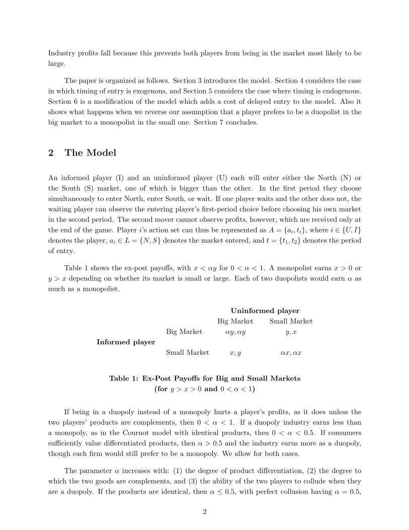
Table 1 shows the ex-post payoffs, with x < αy for 0 < α < 1. A monopolist earns x > 0 ory > x depending on whether its market is small or large. Each of two duopolists would earn α asmuch as a monopolist.

Uninformed playerBig Market Small Market

Big Market αy, αy y, x

Informed playerSmall Market x, y αx, αx

Table 1: Ex-Post Payoffs for Big and Small Markets(for y > x > 0 and 0 < α < 1)

If being in a duopoly instead of a monopoly hurts a player’s profits, as it does unless thetwo players’ products are complements, then 0 < α < 1. If a duopoly industry earns less thana monopoly, as in the Cournot model with identical products, then 0 < α < 0.5. If consumerssufficiently value differentiated products, then α > 0.5 and the industry earns more as a duopoly,though each firm would still prefer to be a monopoly. We allow for both cases.

The parameter α increases with: (1) the degree of product differentiation, (2) the degree towhich the two goods are complements, and (3) the ability of the two players to collude when theyare a duopoly. If the products are identical, then α ≤ 0.5, with perfect collusion having α = 0.5,

2

Bertrand competition having α = 0, and Cournot competition having 0 < α < 0.5. If there isperfect collusion, then 0.5 ≤ α < 1, depending on the degree of product differentiation and productcomplementarity.

We will assume that x < αy; that is, the single-firm duopoly profit in a big market is greaterthan the monopoly profit in a small market. Thus, the follower would be willing to crowd into amarket despite the leader’s presence if he were sure the market was big (though perhaps not if hewere unsure).

The common prior is that both markets are equally likely to be the big market. Before thefirst period, the informed player observes the signal θ ∈ Θ = {N,S} which correct identifies the bigmarket with probability p ≥ 1

2 . As the precision, p, approaches 12 , the signal becomes useless; as

it approaches 1, it becomes perfect. The uninformed player does not observe the informed player’ssignal, but he does know p.

The informed player’s pure strategy is

sI = (tI(θ), aI(θ|tI = t1), aI(θ|tI = tU = t2), aI(θ|tU = t1, tI = t2)) (1)

For given θ, the informed player decides when to enter and whether to follow his signal or not.If aI = θ, we will say that he “uses the signal”. The uninformed player’s strategy is

sU = (tU , aU |(tU = t1), aU |(tI = tU = t2), aU (aI |tI = t1, tU = t2)) (2)

since he observes no signal. We also will allow mixed-strategies for both players.

Let λ be the uninformed player’s belief as to the probability that the informed player usesthe signal in choosing a market. The strategy profile s = {sU , sI} and λ is a perfect Bayesianequilibrium if EπI(sI , sU ) and EπU (sI , sU ) are maximized for given λ and s = {sU , sI} and λ isconsistent with sI in terms of Bayesian updating.

One particular value of p is critical for determining the equilibrium, so let us define:

p ≡ y − xα

(y − x) (α + 1)(3)

It will turn out that for p < p there is a first-mover advantage and for p > p there is asecond-mover advantage.1

We have not yet specified the timing of moves. In Section 3 we will specify which player goesfirst exogenously. In Section 4 we will let the players decide endogenously.

3 Exogenous Timing of Entry

We will start by assuming that the sequence of entry is exogenous, a necessary prelude to theanalysis of endogenous entry. For simplicity, we will assume that if the uninformed player moves

1xxx Is there any meaning to the equation for pbar that we could discuss?

3

without having observed the informed player’s action, he chooses his market by flipping a fair coin.2

The possible exogenous-timing games are (1) the players move simultaneously, (2) the unin-formed player must move first, and (3) the informed player must move first. Proposition 1 sayswhat happens in the equilibrium of each game.

xxx Let us denote the probability that the uninformed player chooses North when he has noinformation by q. Without loss of generality assume that q ≥ .5. q∗

Proposition 1.1) Consider the perfect bayesian equilibria of the entry game when timing is exogenous.1) Suppose entry is simultaneous. If q ≤ q∗ = xxx, the informed player uses his signal and theinformed player is indifferent about which market he chooses.2) Suppose entry is sequential.2-1) If the uninformed player chooses first and q < q∗, he is indifferent about which market hechooses. The informed player uses the signal if p > p, chooses the opposite of the uninformedplayer if p < p, and is indifferent if p = p.2-2) If the informed player chooses first, he uses the signal. The uninformed player imitates him ifif p > p, chooses the opposite of the informed player if p < p, and is indifferent if p = p.

Proof : In the appendix.

Proposition 1 says that when the informed player is the leader, he should use his signal ratherthan try to conceal it by randomization. As proved in the Appendix, there is no pooling or semi-pooling equilibrium. The equilibrium is separating, so the uninformed player can infer the signal θ

perfectly. This is critical in making the players want to delay when θ is relatively precise.

When the informed player is the follower, he has all the less reason to randomize. He knowshe is better informed, so it is natural for him to use the signal, but he must also consider thecompetition that arises when both players are in the same market. Hence, the degree of hisinformation quality affects his decision on whether to use his signal or not. If his informationquality is relatively low, i.e., p < p, he has more reason to worry that the signal is wrong. If theuninformed player already accidentally selected the location signalled by θ, the informed playerwill be reluctant to do the same because of the possibility that both players end up in a smallmarket, yielding the lowest payoff, αx. In this case, the informed player cares more about avoidingcompetition than being in a big market, so he selects the location opposite to what the signalreveals.

On the other hand, if his information quality is relatively high, i.e., p ∈ (p, 1), he has relativelystrong confidence in the correctness of the signal. Even if the uninformed player already chose thelocation signalled by θ, it is better to join him there in what is very likely the best market, becauseαy > x. Hence, regardless of the uninformed player’s choice of location, the informed player uses

2xxx discuss this assumption. Is it innocuous? I we should drop it. It’s not entirely innocuous. I think if there’s

poor information and the players enter simultaneously, then if the Uninformed player always entered Market North

instead of randomizing the players would have higher payoffs than if he randomizes, because they can discoordinate.

4

the signal.

Similar reasoning applies to the uninformed player’s strategy. If the informed player’s infor-mation quality is low, the uninformed player thinks mainly of avoiding competition and divergesin his choice of market, but if the quality is high, he imitates.

From (5), it can be checked that

∂p

∂y=

(α− 1) x

(α + 1) (y − x)2< 0,

∂p

∂x=

(1− α) y

(α + 1) (y − x)2> 0,

∂ (p)∂α

= − x + y

(α + 1)2 (y − x)< 0 (4)

As the large market size y increases, the parameter set for which p ∈ (p, 1) increases. Asy increases, each firm’s payoff from being a duopolist in the large market increases, whereas thepayoff x from being a small-market monopolist stays the same. Hence, as y increases, the informedplayer puts more emphasis on being in the big market and has more reason to follow his signal. Theuninformed player knows this, so he too relies more on the signal– which means that y increases hebecomes more eager to imitate the informed player. On the other hand, as x, the profit when a playeroperates as a monopolist in a small market, increases, the parameter set for which p ∈ (p, 1) falls.The loss from being in a small market decreases and each player’s incentive to avoid competitionin one market grows relative to the incentive to be in a big market. As x rises, whichever player isthe follower becomes more likely to diverge from the leader’s choice. Finally, as α increases, eachfirm’s payoff from being a duopolist in the same market increases. Hence, each firm’s incentive toavoid being in the same market decreases. Hence, the parameter set of p for which the informedplayer sticks to his signal and and the uninformed player wants to imitate the informed player’schoice increases.

3.1 The Expected Payoffs

We wish to make the timing of entry over the two periods endogenous, and this requires settingout the possible payoffs from different timings.

The informed player’s expected payoff is one of two expressions, (7) or (8), depending onwhether the uninformed player will have a chance to observe him or not. If the informed playergoes first and the uninformed player second, the uninformed player can deduce the signal θ perfectly,so his action aU is perfectly predictable. Hence, the informed player’s expected payoff is:

πI(tU , tI) =∑

w∈{N,S}

Pr(w| θ)πI (aI , aU , w) (5)

If, however, the uninformed player has no chance to infer the informed player’s signal, hechooses aU only using his prior, and we have assumed he randomizes 50-50. Hence, the informedplayer’s expected payoff is:

πI(tU , tI) = (0.5)

∑w∈{N,S}

Pr(w| θ)πI (aI , aU = N,w) +∑

w∈{N,S}

Pr(w| θ)πI (aI , aU = S, w)

(6)

5

These two equations cover the four possible combinations of timing. Payoff (7) is for (tU , tI) =(t2, t1) and payoff (8) is for (tU , tI) = (t1, t2), (t2, t2) and (t1, t1).

On the other hand, the uninformed player’s expected payoff is:

πU (tU , tI) =∑

θ∈{N,S}

∑w∈{N,S}

Pr(w, θ)πU (aI , aU , w) (7)

Here, note that his posterior belief should be about the true state w and I’s signal, Pr(w, θ), becauseI has no chance to observe aI and therefore no chance to infer θ before he makes a decision.

Straightforward calculations yield the payoffs in Tables 1 and 2.

tI

t1 t2

t1y+xα−p(y−x)(1−α)

2 , (x−px+py)(α+1)2

(x+y)2 , (x+y)

2

tU

t2 (y + px− py) , (x− px + py) y+xα−p(y−x)(1−α)2 , (x−px+py)(α+1)

2

Table 2: Ex-Ante Expected Payoffs Depending on the Period of Entry When theSignal Is Imprecise: 1

2 < p < p

tI

t1 t2

t1y+xα−p(y−x)(1−α)

2 , (x−px+py)(α+1)2

y+xα−p(y−x)(1−α)2 , (x−px+py)(α+1)

2

tU

t2 α (x− px + py) , α (x− px + py) y+xα−p(y−x)(1−α)2 , (x−px+py)(α+1)

2

Table 3: Ex-Ante Expected Payoffs Depending on the Period of Entry When theSignal Is Precise: p < p < 1

We will use Tables 2 and 3 to find the equilibrium when firms choose their times of entryendogenously.

6

4 Endogenous Timing of Entry

4.1 First-Mover and Second Mover Advantage

Now we will find the conditions under which a player wishes to enter first. Denote i’s ex-anteexpected payoff when he enters as the leader, follower, or simultaneously by πL

i , πFi , and πS

i .

When the signal is imprecise, p < p, Table 2 tells us that:

πSU < πF

U < πLU and πS

I < πFI < πL

I (8)

Each player’s best response as follower is to choose a different location from the leader, eventhough we have assumed that it is better to be a duopolist in the big market than a monopolistin the small market (α > x/y). As the follower, he can operate as a monopolist in one market bydiverging from the leader. This follower behavior is why equation (10) says that a player’s expectedprofits are highest if he is the leader.

If the informed player is the leader, he uses his signal. Since the other player diverges, theinformed player more likely than not ends up as a monopolist in the big market. If he enters asthe follower, however, he should diverge from the uninformed player even if that puts him in themarket he believes is likely to be small. Though if he chooses the signalled market the most likelyoutcome is duopoly in the big market, which is better than duopoly in the small market, it mightbe duopoly in the small market, the worst possible outcome.

The uninformed player’s reasoning is similar. If he enters as the follower, he should choose alocation opposite to the leader, even though he knows that the leader has chosen what is probablythe big market. He would prefer to be the leader, since then he has probability .5 of ending up asa monopolist in the big market, compared to a probability of 1 − p, which is less than .5, as thefollower.

In this weak-information case, the payoff from sharing the market is lower than from beingthe follower: for either player: πS

U < πFU and πS

I < πFI . If p is low, a player’s weak confidence in

the signal (his or the other player’s) is so low that he puts more emphasis on avoiding competition.If both players choose locations simultaneously, they might both end up as monopolists, but theymight not. Acting as the follower is better even if it reduces the chance of being in the big marketbecause it at least prevents the possibility of sharing a small market. The best situation is to bethe leader, the next-best is to be the follower, and the worst case is to enter simultaneously.

When information is precise, and p > p, Table 3 tells us that:

πSU = πL

U < πFU and πL

I < πSI = πF

I (9)

Expression (11) says that if information precision is high, then each player does best as thefollower. The informed player knows that if the uninformed player has a chance to observe his

7

choice, he will choose the same location. For relatively high p, however, he has strong confidencein his signal and the payoff from being either a monopolist or a duopolist in the signalled marketis high. Hence, he enters late to prevent his choice from being revealed and imitated. In fact, hispayoff from simultaneous entry is just as high as from being the follower: πS

I = πFI . If both players

enter simultaneously, the uninformed player still has no chance to observe the informed player’schoice, and the probability the informed player will end up sharing that market is .5.

As for the uninformed player, if the signal is relatively precise then his ideal is to observe theinformed player’s choice and imitate it. If he cannot, he is indifferent between being the leaderor choosing simultaneously: πS

U = πLU . In either case, he has no chance to observe the informed

player’s choice and to infer the signal value. Hence, his expected profits are the same in both cases.

Thus, if information precision is relatively low, there is a first- mover advantage; but if infor-mation precision is high, there is a second- mover advantage. If p < p, a player would prefer to gofirst, but he will delay entry if he thinks the other player will enter first, so as to avoid ending upin the same market. If p > p̄, the uninformed player would like to delay entry in order to observethe informed player’s choice, but if he does delay, the informed player will also delay to preventthat observation. Both end up delaying because of the conflict between two types of second moveradvantage: one from learning and the other from preventing learning.

4.2 The Equilibrium

Using the payoffs from Tables 2 and 3 we can characterize the endogenous timing of entry.

Proposition 2. When entry timing is endogenous, then:1) If information is precise enough, i.e., p > p̄ , there is a second-mover advantage. In equilibrium,the informed player enters in the second period, and the uninformed player is indifferent about whenhe enters.2) If information is not precise enough, i.e., p ≤ p̄, there is a first-mover advantage. There are twopure-strategy equilibria, one for each of two players entering first, and a mixed strategy equilibriumin which the informed player enters without delay with probability z and the uninformed playerenters without delay with probability w:

(z, w) =(

(x− px + py) (α− 1)(2xα− y − x− 2pxα + 2pyα)

,(x− px + py) (α− 1)

(2xα− y − x− 2pxα + 2pyα)

)(10)

Proof : In the appendix.

The signal’s precision is high if p > p. The informed player delays entry and enters in period2 to conceal his information. The uninformed player can only use his prior belief of .5, and hisexpected payoff is the same whenever and wherever he enters.

The signal’s precision is low if p ≤ p. There are two pure-strategy equilibria, in which theplayers enter sequentially into separate markets. Because the information quality is low the players

8

hesitate to rely on it and are most concerned with avoiding competition. One player, at least, hasincentive to delay, but his benefit is not from imitating the leader, but from diverging.

If p ≤ p there is also the mixed strategy equilibrium, in which a player has no safe choice. Sincethe other player is mixing too, if he enters early he might end up competing in the same market,but the same thing could happen if he enters late. Entering early does have the advantage thatif the other player enters late, the leader can preempt the signalled market (if he is the informedplayer) or have a .5 chance of preempting the signalled market (if he is the uninformed player), andthis must be balanced by a higher probability of ending up competing in the same market. Hencethere is some probability of early entry greater than .5 for each player which leaves each of themindifferent about when to enter, and that is the equilibrium mixing probability.

The comparative statics on the mixing probabilities of choosing early entry yield that:

∂z

∂p=

∂w

∂p=

(1− α) (x + y) (y − x)(2xα− y − x− 2pxα + 2pyα)2

> 0 (11)

∂z

∂x=

∂w

∂x=

(α− 1) (2p− 1) y

(x + y − 2xα + 2pxα− 2pyα)2< 0 (12)

∂z

∂y=

∂w

∂y=

(1− α) (2p− 1) x

(2xα− y − x− 2pxα + 2pyα)2> 0 (13)

Inequality (13) says that when information precision increases, both players choose early entrywith higher probability. The increase in information precision p makes choosing the signalled marketmore attractive. For both players to still be willing to choose the unsignalled market, it must bethat choosing the signalled market results in greater probability of undesirable competition. Theway this probability increases is for both of them to increase their probability of early entry untilthe likelihood of competition has risen enough for them to again be indifferent about their timesof entry.

Inequalities (14) and (15) say that the probability of early entry falls with x, the size of thesmall market, and rises with y, the size of the big market. When the size of the small marketincreases, that increases the benefit from waiting and possibly being the only player to enter inperiod 2. As a result, the probability of early entry by the other player does not have to be so highto keep the player indifferent about his time of entry. The effect of an increase in the size of thebig market is parallel: that increases the benefit from possibly being the only early entrant andthe disadvantage of entering early and making the same choice as the other player must increaseto balance that benefit.

Thus, we have shown that whether a first- or a second-mover advantage emerges depends onwhether the preemption effect is dominant, so that the leader does not care about informationleakage, or the information effect is dominant, so the leader’s main concern is to prevent imitation.When knowledge of which market is best is imperfect, the presence of payoff externalities makes

9

preemption possible even when both players would prefer a sure big market duopoly to small marketmonopoly.

3

4.3 Efficiency

Usually in information models, we analyze only ex ante efficiency— whether equilibrium decisionsmaximize the sum of expected payoffs given the information available to the players at the startof the game. Here, however, it is also possible that equilibrium leads to ex post efficiency— thatequilibrium decisions maximize the sum of actual payoffs, as if decisions were made by a socialplanner who had no uncertainty. Here, of course, the uncertainty is over which market is big,and even the informed player’s information is imperfect. Let us use the word “efficient” to mean“maximizing the sum of each firm’s ex-post payoff,” since we have not specified demand preciselyenough to discuss consumer welfare, which will depend on product variety and the loss from amarket being unserved as well as on equilibrium prices.

In our model a player prefers to be a duopolist in the big market than a monopolist in thesmall market, i.e., αy > x. If 2αy > x + y, that is, if α > x+y

2y , it is efficient for both firms to bein the big market, since duopoly profits are large relative to monopoly profits and the differencebetween market sizes is large. Otherwise, efficiency requires that the firms choose different markets.

Suppose the informed player’s information is imprecise ( p > p). From Proposition 2, thepure-strategy equilibria have sequential entry into two different markets. If α < x+y

2y , this is theefficient outcome. Thus, if competition hurts profits enough or the markets are close enough insize, imprecise information results in the firms maximizing industry profits ex post, at least if theequilibrium is in pure strategies.

Ex ante, neither player knows with certainty which is the big market, so the best a plannermaximizing industry profit can do is to either locate both firms at the signalled market or toput them in different markets. Locating in the same market is ex ante efficient if and only if2α(py + (1− p)x) ≥ x + y, which can be expressed in two ways: 4

α ≥ x + y

2[py + (1− p)x]or p ≥ y + x− 2xα

2α(y − x)(14)

If the planner has only the players’ information about which market is big, expected profitsfrom co-location will naturally be lower than when he knew perfectly which was big. Thus, thedegree of product differentiation or duopoly cooperation α has to be bigger than in Proposition 3.

3 xxx Add a proposition saying that the informed player always benefits from greater precision, even if it pushes

him over the critical threshold.4 When both are in the same market, it is the big market with probability p and the small market with probability

1 − p. Hence, πI = πU = pαy + (1 − p)αx and πI + πU = 2α (py + (1− p)x). If both are in the separate market,

πI+πU = x+y. Finally, locating both firms in the same market is ex ante efficient if and only if 2α(py+(1−p)x) ≥ x+y.

10

That degree will now depend on the quality of information, p now too, as shown in equation (16).Proposition 4 characterizes ex-ante efficiency using both α and p.

Proposition 4. Ex-ante efficiency depends on the ratio of duopoly profit to monopoly profit (α)and the quality of information (p) as follows.1) Suppose that duopoly profit is low relative to monopoly profit, so x

y < α < x+y2y . Then all pure-

strategy equilibria are efficient.1-1) If p < p, both pure strategy equilibria are efficient and the mixed strategy equilibrium is not.(A1 in Figure 1)1-2) If p < p, all equilibria are efficient. (A2 in Figure 1)2) Suppose that duopoly profit is high relative to monopoly profit, so x+y

2y < α. Then improvedinformation can lead to the inefficient equilibria.2-1) If p < p, both pure strategy equilibria are efficient but the mixed strategy equilibrium is not.(A5 in Figure 1)2-2) If p < p < y+x−2xα

2α(y−x) , all equilibria are efficient. (A4 in Figure 1)

2-3) If y+x−2xα2α(y−x) < p , all equilibria are inefficient. (A3 in Figure 1)

Proof : In the appendix.

Figure 1: Information Quality, Market Size, and Efficiency for x = 1 and y = 5(see end of paper)

Figure 1 illustrates the possible equilibrium regions for the case where the monopoly profitsare x = 1 in the small market and y = 5 in the large market. The values of p lie between .5 and1, and values of the duopoly/monopoly profit ratio lie between x/y and 1, given our assumptionthat the duopoly profit in the big market is greater than the monopoly profit in the small market,i.e., αy > x. The vertical line represents the boundary condition that α = x+y

2y and the two slopinglines represent p = p and p = y+x−2xα

2α(y−x) .

If we ignore mixed-strategy equilibria, the parameter set of α and p for which the equilibriaare efficient (areas A1, A2, A4 and A5) increases as the information quality declines and duopolyrelative to monopoly profits rise. In area A3, where the duopoly competition is not severe, ex-anteefficiency requires both firms to locate in the market signaled as big, but the informed player delaysto conceal his greater information precision. The uninformed player enters randomly and theymight end up in separate markets, which is inefficient. In this sense, more accurate informationhurts efficiency.

11

5 Modifications to the Model

5.1 What if It Is Costly to Delay Entry?

We have assumed that entering in the first or the second period have the same direct cost. In fact,we can imagine the cost being higher in either direction— that entering early is more costly, or thatentering late is more costly. A higher cost of early entry does not change the model in interestingways. It reinforces the strong-information equilibrium of delayed entry and it would not modifythe weak-information sequential equilibria unless the direct cost were very high.

What is more interesting is when there is a cost to delay. Such a cost has little impact wheninformation is weak, but with strong information the pure strategy equilibrium disappears and isreplaced by a mixed strategy equilibrium. In showing this, we will also be able to show when theuninformed player’s second mover advantage from learning is stronger than the informed player’sone from preventing learning.

Let us assume that each player has the same exogenous delay cost c of entering in the secondperiod. Then, Propositions 5 and 6 characterize the equilibrium.

Proposition 5. Suppose that 12 < p < p̄, and the entry in the second period incurs a cost of c > 0.

1) If c > c∗, the unique equilibrium is (tU , tI) = (t1, t1).2) If 0 < c < c∗, there exist two pure strategy equilibria (tU , tI) = (t1, t2) , (t2, t1) and one mixedstrategy equilibrium (z, w) where z = Pr(tU = t1) and w = Pr(tI = t1).The values of z, w, and c∗ are z = w = (px−x−2c−py+xα−pxα+pyα)

(2xα−y−x−2pxα+2pyα) and c∗ = (y+px−py−xα+pxα−pyα)2 .

Proof: In the appendix.

Proposition 5 covers the weak-information case. If the delay cost c is low enough, the equilib-rium is similar to what we found in Proposition 2 for c = 0: two equilibria with sequential entryand a mixed strategy equilibrium. Only the mixing probability changes, to depend on c, becausenow late entry has fallen in attractiveness. If, on the other hand, c is large, both players enter earlyin the unique equilibrium. The critical value c∗ equals the cost of losing the chance to observe andof entering simultaneously instead, so c∗ = πF

U −πSU = πF

I −πSI (an equality apparent from Table 2).

If delay’s direct cost is less than its equilibrium benefit, i.e., c < c∗, the equilibrium in which eachplayer gives more weight to avoiding competition in the same market can be sustained. Otherwise,both players enter simultaneously in period 1.

We will soon proceed to the strong-information case, but first let us make some observationson which player gains most from delay. Let dU and dI denote each player’s gain from being thefollower instead of the leader in a game with an exogenous sequence of moves.

Lemma 2. Suppose that p̄ < p < 1. There exists a value α∗ = x+y2y ∈

(xy , 1

)such that:

1) If α ∈(

xy , α∗

), then dU < dI for all p ∈ (p̄, 1) . That is, the uninformed player has less benefit

12

from delay.2) If α ∈ (α∗, 1), for p ∈

(p̄, y+x−2xα

2α(y−x)

), dU < dI and for p ∈

(y+x−2xα2α(y−x) , 1

), dU > dI . For

information weak enough, the informed player has the bigger benefit from delay, but for stronginformation, the uninformed player does.

Proof : In the appendix.

The value dU is the gain from delay that allows learning (imitating the choice of the informedplayer) and the value dI is the gain from delay that preventing learning (preventing the uninformedplayer’s imitation). If duopoly competition is severe, so α is small, the dU < dI and the gainfrom preventing learning is the greater. This makes sense because strong duopoly competitionreduces the imitator’s benefit to imitation and increases the leader’s cost from it. If competitionis not so severe, the benefit from discovering the signalled market might dominate the negativepayoff externality. The learning benefit does not outweigh the negative payoff externality if theinformation is relatively weak (or perhaps we should say “moderately strong,” since we are inthe strong-information case throughout Lemma 2). Learning does outweigh the externality if theinformation is strong enough, so in that case it is the uninformed player whose benefit from delayis the greater.

Lemma 2 is interesting in itself, but it also is useful for characterizing the equilibrium, sincethe delay cost cutoffs will differ for each player, unlike in the weak-information case, as Proposition6 says.

Proposition 6. Suppose that αy > x , p̄ < p < 1 and the delay cost is strictly positive: c > 0 .1) If c > Max{dU , dI}, the two players both enter in period 1;2) If Min{dU , dI} < c < Max{dU , dI}, the player with the lowest delay benefit enters in period 1and the other enters in period 2;3) If c < Min{dU , dI}, the unique equilibrium is a mixed strategy equilibrium in which the playersrandomize over their period of entry.

The first two cases are simple. The interesting case is the third one where c is positive butbelow the delay gains of either player. In this case, the unique equilibrium is a mixed strategies. Tosee this, consider the pure strategy combinations. Suppose (tU , tI) = (t1, t1). Then, the uninformedplayer has an incentive to deviate to tU = t2 in order to observe the informed player’s choice. If(tU , tI) = (t2, t1), however, the informed player has an incentive to deviate to tI = t2 to preventthe uninformed player from observing his choice. If they both enter in the second period, so(tU , tI) = (t2, t2), the uninformed player has incentive to deviate to tU = t1 because delay does notallow him to observe the informed player’s move, but it does incur cost c. But if (tU , tI) = (t1, t2),the informed player might as well deviate to enter in the first period, since in this strong-informationcase he will follow his signal anyway and so his simultaneous move payoff is the same as his sequentialmove payoff except for the delay cost c. Thus, there is no pure strategy Nash equilibrium.

Proposition 6 says that in the strong-information case, the asymmetry between the two kinds

13

of second-mover advantage, for learning and for preventing learning, can lead to sequential equilibriainstead of both players’ delaying as we found when c = 0 in Proposition 2. From Lemma 2, theinformed player will be the last to enter for moderate values of c if duopoly competition is intenseor information quality is only moderately strong, because his benefit from preventing competitionwill be greater than the uninformed player’s benefit from learning. If duopoly competition is not sointense and information quality is very strong, then the uninformed player will be the last to enterbecause his gain from learning outweighs the loss from duopoly pricing. If the value of c is smallenough, however, both players would be willing to pay it to acquire a second-mover advantage. Ifthey both do delay, however, they will enter simultaneously, which is no better for the uninformedplayer than entering first and which is worse taking into account his delay cost c, so he will not delayunless there is some probability that the informed player will enter early. Entering simultaneouslyin period 1, however, is just as good for the informed player as delaying entry to period 2, so theinformed player will not delay unless there is some probability that the uninformed player will enterlate. Hence, a mixed strategy equilibrium results.

The importance of having only a mixed-strategy equilibrium can be overrated, since if c is smallit will take only a small probability of each player entering early to support the equilibrium andit will look much like the pure-strategy equilibrium when both players delay with certainty. Whatis more interesting is the asymmetric second-mover advantages from learning and from preventinglearning: that bigger negative payoff externalities and worse information tend to make the secondmover advantage from preventing learning bigger than that from the learning itself, in contrast tothe conclusion in Yoon (2006).

Recall that in the former section, we checked that when duopoly competition is not severe,more accurate information can lead to inefficient equilibria because of the informed player’s incentiveto conceal information. The corresponding conditions are α ∈

(x+y2y , 1

)and p ∈

(y+x−2xα2α(y−x) , 1

). Now

note that according to Lemma 2, if a delay of entry is costly, for these parameter sets of α and p,dU > dI . Then, if dI < c < dU , the informed player should act as the leader and the uninformedplayer has a chance to observe his choice and therefore imitate it. Hence, the ex-ante efficiencycan be attained. That is, when the duopoly competition is not severe and the informed player’sinformation is quite accurate, the moderate but not too high delay cost can resolve the inefficiencyand therefore function as a means to increases welfare.

5.2 What if a Monopolist in the Small Market Would Have Higher Profits than

a Duopolist in the Big Market? (αy < x)

So far we have assumed that a player would rather be a duopolist in the big market than amonopolist in the small market. Then what would happen if we assume instead that αy < x?In this case, we can easily conjecture that the new assumption reduces the value of being in thebig market as a duopolist, so the first mover advantage of preemption now outweighs the secondmover advantage of learning for the uninformed player. The learning motive, in fact, collapsescompletely, because obtaining the benefit of learning requires that the follower become a duopolist,which is inferior to being a monopolist even if the identity of the big market is learned perfectly.

14

Therefore, the equilibrium we can expect is same as the one derived when αy < x and the qualityof information is poor. The detailed analysis is analogous to that used in the former sections, sowe skip it here.

Proposition 7 Suppose that αy < x , so a firm prefers being a monopolist in a small market tobeing a duopolist in a big market. Then, for all p ∈

(12 , 1

), there exist two pure-strategy equilibria

(tU , tI) = (t2, t1), (t1, t2) and one mixed-strategy equilibrium (z, w) where z = Pr(tU = t1) andw = Pr(tI = t1). The values (z, w) are identical to those found earlier in equation (15).

The sequential entry in both pure equilibria is based on each player’s incentive to avoid thecompetition in the same market. The mixed strategy equilibrium in which players randomize theirentry date survives, but only because the reason for the mixing is not to learn or prevent learning,but the uncertainty mixing creates over which market to choose to avoid competition. Also, it canbe checked that the pure strategy equilibria are ex-post efficient.5

Proposition 8. Suppose that αy < x, so a player prefers being a monopolist in the small marketto being a duopolist in the big market. Then, for all p ∈

(12 , 1

), the two pure strategy equilibria

(tU , tI) = (t2, t1), (t1, t2) are ex-post efficient.

Proof : What is efficient depends on α. If α < x+y2y , the socially efficient case is the one where each

player operates as separate monopolists. If α > x+y2y , it is the one where both players compete in

the big market. Our condition is αy < x where xy < x+y

2y . Hence, if αy < x, the socially efficientcase is the one where each player operates as a monopolist in a separate market. Recall that eachplayer’s best response as the follower is to choose a different location from that of the leader. Also,in both pure equilibria, both players’ timings of actions are sequential always. Therefore, both purestrategy equilibria are ex-post efficient. �

6 The Literature

The Stackelberg model [Heinrich von Stackelberg [1934]) is an early model of first-mover advantage,a sequential-move quantity game in which the first mover, by committing to a large quantity, gainsa profit advantage over the second mover compared to in the simultaneous-move Cournot model.Articles by Esther Gal-or (1985, 1987), J. Hamilton & S. Slutsky (1990), and Paul Klemperer &Margaret Meyer (1986) analyze variations of this game. Anderson & Engers (1994), in particular,

5 As an example, consider the Cournot model with linear demand and identical products. In that model, the

duopoly profit per player is less than the half of the monopoly profit, i.e., α < 12. Proposition 3 told us that when the

signal of the more-informed player is relatively weak and xy

< α < x+y2y

then both pure strategy equilibria are ex-post

efficient. That case applies in the linear Cournot model, since 12

< x+y2y

. Proposition 6 adds that the equilibria are

ex-post efficient even if α < xy. Thus, in the linear Cournot model with weak information, ex-post efficiency is always

attained in the pure strategy equilibria. In conditions of severe enough competition, unlike our main case where

duopoly was relatively attractive, improved information does not cause a shift an equilibrium with lower industry

profits.

15

looks at what happens when the timing of entry is endogenous. Two articles by Eric Van Damme& S. Hurskens (1999, 2004) look at whether a player would prefer to move first or second in variousother games in which both player are already in the market and the choice variables are priceor quantity. With linear quantity setting in a price-setting duopoly game when the timing ofcommitment is decided endogenously, they show that in the risk- dominant equilibrium, the high-cost player will choose to wait and the low-cost player will emerge as the endogenous Stackelberg andprice leader. Although the timing of action is decided endogenously, in both models, informationalexternalities do not play any role.

Similarly, there is a large literature on the war of attrition and pre-emption games in whichplayers do not learn about the market as a result of entry. Argenziano & Schmidt-Dengler (2008)provides a good survey of pre-emption games, and Brunnermeier & Morgan (2004) gives a gooddiscussion of “clock games”. Bouis, Huisman & Kort (2006) adds uncertainty in the form of changesin market demand, but this is observed even without entry, and its main interest is in changing theintervals between entry.

Those articles are about commitment, in a setting without information about the market beingrevealed by entry. Gal-Or (1987) shows that a player with superior information on demand mayprefer ex ante to have to move simultaneously rather than first, because otherwise if demand isstrong the player will reveal that to its rival by its choice of high output (though George Mailath[1993] shows that if the well- informed player has the option of moving first, it will always takethat option, since to delay reveals that it is trying to hide strong demand). Hans-Theo Normann(1997, 2002) also looks at what happens when one duopolist is better informed when he makes hisquantity decision. Levin & Peck (2003) looks at a different kind of asymmetric information: firmsdiffer in their entry cost, and must decide when to enter a natural monopoly in a variant of thegrab-the- dollar game.

In all these models, the players are making decisions about how hard to compete in one market,not whether to compete at all, and the quality of the informed player’s information is unimportant.In the present paper, two major concerns will be what happens when the well- informed player turnsout to be wrong after all (since he will not have perfect information), and whether it is efficient tohave entry in two markets rather than one. Also, the decisions will be binary– to enter a marketor not– rather than a continuous quantity or price decision, so we can focus strictly on the orderof moves rather than on distortions arising from entry deterrence tactics.

In other models, players are symmetric but there is uncertainty and the first player’s movecreates new information. In Rafael Rob (1991), entry has an informational and payoff externality,but the players are not asymmetrically informed, and the market is competitive. The timing ofactions is given exogenously, and the focus is on the second mover’s advantage from seeing whathappens to the first mover. Rob does not analyze the possible advantage to moving second toprevent the other player from learning. Patrick Bolton & Chris Harris, Midori Hirokawa & DanSasaki (2001) and Heidrun Hoppe (2000) (see too Heidrun Hoppe & Ulrich Lehmann-Grube (2001))also look at what happens when the first mover’s move reveals something about the state of theworld, as opposed to something about the first mover’s information. In the present paper, what

16

the second mover gets from observing the first mover’s choice is not direct information about theunknown true state. Market quality is only revealed after both players have moved, so there isno “Who will bell the cat?” problem. Instead, the players are asymmetrically informed, and oneplayer’s move reveals something about his information.

Appelbaum and Lim (1985), Spencer and Brander (1992), and Somma (1999) also deal withthe topic of market preemption and delay. The main focus of these papers is the tradeoff betweenprecommitment and delay’s flexibility in a situation where uncertainty is resolved exogenously overtime. Although precommitment may give market dominance, it can also hurt profits because therealized true state might not be fit with an early decision. Delay has option value; the choice canbe made later after uncertainty is resolved. Hence, a firm needs to decide which is more important,precommitment or flexibility, which can be interpreted as a decision on the allocation of investmentin the various environments. This model is distinct from the flexibility-precommitment literaturebecause, in this model, the uncertainty is not resolved until both firms make their choices. Delaydoes not provide protection against uncertainty. On the other hand, a follower might learn fromthe leader’s choice by being able to infer the leader’s superior information. Our focus, in fact, ison that informational externality.

Another setting has players asymmetrically informed, but without any payoff externality.Christopher Chamley and Douglas Gale (1994) and Jianbo Zhang (1997) discuss strategic delayand the endogenous timing of action when only informational externalities are present and there isno negative payoff externality from one player choosing the same action as another, though thereis some intrinsic cost to delay. In Chamley and Gale (1994), a player has an incentive to delayhis action to observe other players’ decisions for information updating. Zhang (1997) links thisresult to informational cascades. He concludes that the most-informed player is least willing towait, because he has the least to learn than other players. He acts as the leader, and other playersmimic him immediately. In these models, although the action timing is endogenous, there are notpayoff externalities from actions. Each player’s main concern is whether the cost of delay is worthlearning other players’ information.

Whether it is best to move first or second has received attention outside of economics too. Anexample in the marketing is the empirical study by Venkatesh Shankar, Gregory Carpenter andLakshman Krishnamurthi (1998); examples from management strategy are the articles by MarvinLieberman and David Montgomery (1988, 1998).

In the present paper, the timing of actions is endogenous and the action has both informationaland payoff externalities. Two papers look at this combination.

In Yoon (2006) there is also a less-informed player who delays to learn and a better-informedplayer who delays to prevent learning in a war of attrition. Although both players benefit frombeing the follower, the gain from learning is greater than from preventing learning, so the leader isthe better-informed player. The conclusion is different from the present paper’s because the payoffstructure is different. Yoon (2006) models reputation and career concerns rather than entry. Hence,although the best outcome is to be correct alone (as here), the worst outcome is to be incorrect

17

alone, not to be incorrect in company with the other player. In a model of market entry, the worstoutcome is for both players to end up in a small market, having made the same mistake. Thatpossible payoff is crucial to why the quality of information determines whether the advantage is tothe first or the second mover. It also is why the relative magnitude of the gain from learning andthe gain from preventing learning will depend on the business environment in the present model.

Frisell (2003), like the present paper, asks who will enter first, a less informed or a betterinformed player. He uses a continuous-time model of the war of attrition: who is willing to waitthe longest, when delay means a loss in profits? He finds, if we may adapt his model to ourpaper’s context, that if a firm’s duopoly profit is higher than its monopoly profit (a case we do notconsider in this paper) or just a little lower, the informed player enters first. If duopoly profit isenough lower, however, the informed player waits longer. What matters is the ratio of duopoly tomonopoly profits, not the degree of information superiority (a degree which will play an importantrole in the present paper). In contrast to the model to be laid out here, delay costs are crucialto the entry decision, but delay can be infinitely long. Here, there will be a deadline for entry.Players must decide to enter either early, or late. One player cannot simply outwait the other–if he waits, the result will be simultaneous choices. If both players want to move late, they cando so, but they will be simultaneous movers. As a result, in our model a player who moves latemust be concerned about ending up in the same market as his rival by accident, even if he hasprevented purposeful imitation. The use of discrete instead of continuous time is merely a matterof modelling convenience, but the existence of an entry deadline is a substantive difference betweentwo papers. A deadline models either the closing of the entry opportunity or the necessity ofchoosing which market to enter without having observed the other player’s decision. Closing ofthe entry opportunity is important if additional firms can enter after a certain date, or if demandor regulatory conditions might become less favorable. Observation of the entry decision becomesdifficult if observable entry must be preceded by lengthy planning and purchase of site-specificinputs. Indefinite delay to avoid simultaneous entry then does not incur a stationary delay cost;it risks a sharp loss. We will find, in contrast to Frisell, that even if industry profits suffer heavilywhen both players are in the same market, the informed player may decide to move first if he is notmuch better informed. Frisell does not look at industry profits, but we will see that the possibilityof simultaneous entry also has implications for them.

7 Concluding Remarks

Often, a player must make a choice knowing that the choice may be imitated by another player.This choice might be of a new geographic market, as in our model, or of a new product, whichcould be modelled with exactly the same mathematics. Moving first may or may not deter entryinto the market by the rival player, but it certainly will reveal information. Hence, in a setting ofendogenous timing of entry, the decision on the timing of entry can be interpreted as the decision onthe flow of his private information. Of course, how is revealed information used by the other playeraffects the decision on the timing of entry. If the informed player’s information is not strong, theattempt by both players to avoid crowding into one market results in the pure strategy equilibrium

18

in which they operate as monopolists in separate markets. On the other hand, if the informedplayer’s information is relatively valuable, the rival player wants to learn it and imitate his choice.Hence, an informed player may well choose to delay entry to prevent imitation, which results in anequilibrium in which no learning is available. This kind of strategic delay by both players increasesthe probability that they end up in the same market, so the good information that causes the delaycan actually end up reducing industry profits.

19

8 Appendix

In the Appendix, ”I ” denotes the ”informed player” and ” U ” denotes the ”uninformed player”.

8.1 Proof of Proposition 1

First, consider the case where the entry is simultaneous. In this case, it is obvious that U choosesrandomly between N and S because no additional information is observable except his prior beliefthat Pr (w = N) = Pr (w = S) = .5. Now, as for the best response of I, without loss of generality,assume that θ = N . Then,

EπI [aI = N, aU , w] =∑

w∈{N,S}

Pr(w| θ = N) [.5πI (·, aU = N) + .5πI (·, aU = S)] (A1)

=12

(x− px + py) (α + 1)

EπI [aI = S, aU , w] =∑

w∈{N,S}

Pr(w| θ = N) [.5πI (·, aU = N) + .5πI (·, aU = S)] (A2)

=12

(y + px− py) (α + 1)

where (A1) is the expected payoff when informed player uses his signal and (A2) is the one whenhe deviates from it. Then:

EπI [aI = N, aU , w]− EπI [aI = S, aU , w] =12

(y − x) (2p− 1) (α + 1) > 0 (A3)

So, I’s best response is aI = N . This implies that if θ = S, it should be that aI = S. Hence, I’sbest response is to use his signal.

Second, consider the case where the entry is sequential.

1) What if U moves first? There are two cases depending on whether I’s signal equals U’saction or not: θ = aU and θ 6= aU .Case i: θ = aU . Without loss of generality, assume that θ = aU = N . Then, under the posteriorbeliefs Pr(w = N | θ = N) = p and Pr(w = S| θ = N) = 1− p,

EπI(aI = θ, aU , w) =∑

w∈{N,S}

Pr(w| θ = N)πI (aI = θ, aU , w) = p (αy) + (1− p) (αx) (A4)

EπI(aI 6= θ, aU , w) =∑

w∈{N,S}

Pr(w| θ = N)πI (aI 6= θ, aU , w) = p (x) + (1− p) (y) (A5)

where (A4) is I’s expected payoff when he uses his signal and (A5) is the one when he deviatesfrom his signal. Then, if p R (xα−y)

(α+1)(x−y) = p, EπI(aI = θ, aU , w) R EπI(aI 6= θ, aU , w) wherep ∈

(12 , 1

).

20

Case ii: θ 6= aU . Without loss of generality, assume that θ = N and aU = S. Then, under theposterior beliefs Pr(w = N | θ = N) = p and Pr(w = S| θ = N) = 1− p,

EπI(aI = θ, aU , w) =∑

w∈{N,S}

Pr(w| θ = N)πU (aI = θ, aU , w) = py + (1− p) x (A6)

EπI(aI 6= θ, aU , w) =∑

w∈{N,S}

Pr(w| θ = N)πU (aI 6= θ, aU , w) = p (αx) + (1− p) (αy) (A7)

Thus, if p > (yα−x)(α+1)(y−x) , (A6) > (A7) and if p < (yα−x)

(α+1)(y−x) , (A6) < (A7). However, (yα−x)(α+1)(y−x)−

12 =

(α−1)(x+y)2(α+1)(y−x) < 0. Hence, for all p ∈

(12 , 1

), (A6) > (A7).

Therefore, I’s best response is as follows: If p > (xα−y)(α+1)(x−y) = p, regardless of U’s choice in round

1, I uses his signal. On the other hand, when p < p, if θ = aU , he deviates from his signal and ifθ 6= aU , he uses his signal.

2) What if I moves first? This is the harder case, because what U observes is aI , not θ. As θ

is private information, U does not know whether I follows his signal or not in deciding a location.Here, note that whether θ = N or θ = S, both cases are ex-ante symmetric. Hence, intuitively apooling strategy or semi-separating strategy cannot constitute equilibrium. The following analysisshows that the separating strategy which constitutes equilibrium is the one which implies that Ifollows his signal in selecting location.

U must assign some belief λ for that aI = θ. In a pure strategy equilibrium, this belief isλ ∈ {0, 1}. As a first step in looking at beliefs, suppose that U’s belief λ does equal zero or one.Suppose U believes aI = θ, i.e., λ = 1. Without loss of generality, let aI = N . U’s posterior beliefsare Pr(w = N | θ = N) = p and Pr(w = S| θ = N) = 1− p , so

EπU (aI = θ, aU , w) =∑

w∈{N,S}

Pr(w| θ = N)πU (aI = aU , w) = p (αy) + (1− p) (αx) (A8)

EπU (aI 6= θ, aU , w) =∑

w∈{N,S}

Pr(w| θ = N)πU (aU 6= aI , w) = p (x) + (1− p) (y) (A9)

Next, suppose U believes that aI 6= θ, i.e., λ = 0. Then, U’s posterior beliefs are Pr(w = N | θ =S) = 1− p and Pr(w = S| θ = S) = p, so

EπU (aI = θ, aU , w) =∑

w∈{N,S}

Pr(w| θ = S)πU (aI = aU , w) = (1− p) (αy) + p (αx) (A10)

EπU (aI 6= θ, aU , w) =∑

w∈{N,S}

Pr(w| θ = S)πU (aI 6= aU , w) = (1− p) (x) + p (y) (A11)

More generally, I might mix, so U’s belief that aI = θ would be λ ∈ [0, 1]. Then

EπU (aI = θ, aU , w)

(A12)

= λ

∑w∈{N,S}

Pr(w| θ = N)πU (aI = aU , w)

+ (1− λ)

∑w∈{N,S}

Pr(w| θ = S)πU (aI = aU , w)

21

EπU (aI 6= θ, aU , w)

(A13)

= λ

∑w∈{N,S}

Pr(w| θ = N)πU (aU 6= aI , w)

+ (1− λ)

∑w∈{N,S}

Pr(w| θ = S)πU (aI 6= aU , w)

Consequently,

λ T λ∗ =⇒ EπU (aU = aI , w) T EπU (aU 6= aI , w) (A14)

where λ∗ = (x−px+py−yα−pxα+pyα)(y−x)(2p−1)(α+1) . We will state and prove Lemma A.1, included only here in the

Appendix to help prove Proposition 1.

Lemma A.1. Suppose that I chose a location as the leader.a) Suppose that p ∈

(12 , p

). Then, for all λ ∈ [0, 1], U diverges from I’s choice.

b) Suppose that p ∈ (p, 1). Then, there exists λ∗ ∈ (0, 1) such that if λ ∈ (λ∗, 1], U imitates I’schoice, if λ ∈ [0, λ∗) , U diverges from I’s choice, and if λ = λ∗, U is indifferent between imitatingand diverging.

Proof of Lemma A.1. We start by checking whether λ∗ ∈ (0, 1) or not. First, for λ∗, ifp > yα−x

(y−x)(α+1) , λ∗ > 0 and if p < yα−x(y−x)(α+1) , λ∗ < 0. However, yα−x

(y−x)(α+1) −12 = (α−1)(x+y)

2(α+1)(y−x) < 0.

So, for p ∈(

12 , 1

), λ∗ > 0. Also, from λ∗−1 = (y+px−py−xα+pxα−pyα)

(α+1)(2p−1)(y−x) , if p > y−αx(y−x)(α+1) , λ∗ > 1 and

if p < y−αx(y−x)(α+1) , λ∗ < 1 where y−αx

(y−x)(α+1) ∈(

12 , 1

). Therefore, we can summarize as follows: a) If

p ∈(

12 , y−αx

(y−x)(α+1)

)then for all λ ∈ [0, 1], EπU (aU = aI) < EπU (aU 6= aI). b) If p ∈

(y−αx

(y−x)(α+1) , 1)

then if λ > λ∗, EπU (aU = aI) > EπU (aU 6= aI), if λ < λ∗ , EπU (aU = aI) < EπU (aU 6= aI), and ifλ = λ∗, EπU (aU = aI) = EπU (aU 6= aI). �

Let us now return to the informed player’s best response, which we can derive using LemmaA.1. In following, we denote y−αx

(y−x)(α+1) ≡ p̄. Without loss of generality, assume θ = N . Then, I’sposterior beliefs are Pr(w = N | θ = N) = p and Pr(w = S| θ = N) = 1− p.

First, assume that p ∈(

12 , p

). In this case, U chooses a location different from I’s choice for

all λ ∈ [0, 1]. Then

EπI (aI = θ, aU , w) =∑

w∈{N,S}

Pr(w| θ = N)πU (aI = θ 6= aU , w) = p (y) + (1− p) (x) (A15)

EπI (aI 6= θ, aU , w) =∑

w∈{N,S}

Pr(w| θ = N)πU (aI 6= θ = aU , w) = p (x) + (1− p) (y) (A16)

andEπI(aI = θ, aU , w)− EπI(aI 6= θ, aU , w) = (y − x) (2p− 1) > 0 (A17)

Thus, I’s best response is to choose the location following his signal, which is consistent to U’sbelief that λ ∈ [0, 1].

22

Next, let p ∈ (p, 1). First, suppose λ > λ∗, so U imitates I. Then:

EπI (aI = θ, aU , w) =∑

w∈{N,S}

Pr(w| θ = N)πU (aI = θ = aU , w) = p (αy) + (1− p) (αx) (A18)

EπI (aI 6= θ, aU , w) =∑

w∈{N,S}

Pr(w| θ = N)πU (aI = aU 6= θ, w) = p (αx) + (1− p) (αy) (A19)

and:EπI(aI = θ, aU , w)− EπI(aI 6= θ, aU , w) = α (y − x) (2p− 1) > 0 (A20)

Hence, I’s best response is to choose a location following the signal, which is consistent to U’s beliefthat λ > λ∗.Second, suppose λ < λ∗, so U diverges from I’s choice. Then, from (A15) - (A16), I chooses alocation following the signal. However, this is inconsistent to U’s belief that λ < λ∗ . Hence, thiscase is excluded.Third, suppose λ = λ∗, so , U is indifferent between imitating and diverging from aI . Suppose σU

is the probability that U imitates I’s choice. Then:

EπI (aI = θ, aU , w)− EπI (aI 6= θ, aU , w)

(A21)

= σ

∑w∈{N,S}

Pr(w| θ = N)πU (aI = aU , w)

+ (1− σ)

∑w∈{N,S}

Pr(w| θ = N)πU (aI 6= aU , w)

−

σ

∑w∈{N,S}

Pr(w| θ = N)πU (aI = aU , w)

+ (1− σ)

∑w∈{N,S}

Pr(w| θ = N)πU (aI 6= aU , w)

= (y − x) (2p− 1) (ασ − σ + 1)

It can be checked that EπI (aI = θ, aU , w) = EπI (aI 6= θ, aU , w) only at σ = 11−α . But 1

1−α /∈[0, 1] for 0 < α < 1. Hence, there exists no σ ∈ [0, 1] which yields EπI (aI = θ, aU , w) =EπI (aI 6= θ, aU , w).

Finally, I’s best response in round 1 is to act so as to reveal his signal perfectly. Since U’sbelief must be correct in equilibrium, it must be λ = 1 and his strategy must be to diverge fromaI if p < p and to imitate aI if p > p, as stated in Proposition 1. �

8.2 Proof of Proposition 2

Denote z = Pr(tU = t1) and w = Pr(tI = t1). Also, let Ei(ti = tk) denote i’s expected payoffwhen he acts at round k, where i ∈ {I, U} and k ∈ {1, 2}.

23

(1) Consider the case in which 12 < p < p. From Table 2:

EU [tU = t1] = w

(−(p (y − x) (1− α)− y − xα)

2

)+ (1− w)

(12

(x + y))

(A22)

EU [tU = t2] = w (y + px− py) + (1− w)(−(p (y − x) (1− α)− y − xα)

2

)(A23)

Thus:

EU [tU = t1]− EU [tU = t2] = w

(xα− 1

2y − 1

2x− pxα + pyα

)+

(12

)(x− px + py) (1− α)

(A24)For p ∈

(12 , p

), xα− 1

2y − 12x− pxα + pyα < 0. Hence U’s best response for given w is:

w < w∗ =⇒ z = 1, w = w∗ =⇒ z ∈ [0, 1], w > w∗ =⇒ z = 0 (A25)

where w∗ = (x−px+py)(α−1)(2xα−y−x−2pxα+2pyα) ∈ (0, 1). Returning to Table 2 for I’s payoffs:

EI [tI = t1] = z

(12

(x− px + py) (α + 1))

+ (1− z) (x− px + py) (A26)

EI [tI = t2] = z

(12

(x + y))

+ (1− z)(

12

(x− px + py) (α + 1))

(A27)

Thus:

EI [tI = t1]− EI [tI = t2] = z

(xα− 1

2y − 1

2x− pxα + pyα

)+

12

(x− px + py) (1− α) (A28)

Equation (A28) is identical to (A24). Hence, I’s best response for z is the same as U’s one for w:

z < z∗ =⇒ w = 1, z = z∗ =⇒ w ∈ [0, 1], z > z∗ =⇒ w = 0 (A29)

Finally, the intersection of the players’ best response functions (A25) and (A29) yields that (z, w) =(0, 1), (1, 0) and (z∗, w∗) – there exist two pure strategy equilibria (tU , tI) = (t2, t1), (t1, t2) and onemixed strategy equilibrium (z, w) =

((x−px+py)(α−1)

(2xα−y−x−2pxα+2pyα) ,(x−px+py)(α−1)

(2xα−y−x−2pxα+2pyα)

).

(2) Consider the case in which p < p < 1. Table 3 gives U ’s payoffs as:

EU [tU = t1] = −(p (y − x) (1− α)− y − xα)2

(A30)

EU [tU = t2] = w (α (x− px + py)) + (1− w)(−(p (y − x) (1− α)− y − xα)

2

)(A31)

Thus:EU [tU = t1]− EU [tU = t2] =

12w (p (− (y − x) (α + 1)) + y − xα) (A32)

Note that for p < p < 1, p (− (y − x) (α + 1)) + y − xα < 0. So U’s best response for w is:

w < 0 =⇒ z = 1, w = 0 =⇒ z ∈ [0, 1], w > 0 =⇒ z = 0 (A33)

Next, Table 3 gives I’s payoffs as:

EI [tI = t1] =z

(12

(x− px + py) (α + 1))

+ (1− z) (α (x− px + py)) (A34)

EI [tI = t2] =12

(x− px + py) (α + 1) (A35)

24

Thus:

EI [tI = t1]− EI [tI = t2] = z

(12

(x− px + py) (1− α))

+12

(x− px + py) (α− 1) (A36)

Hence, I’s best response to the uninformed player is:

z > 1 =⇒ w = 1, z = 1 =⇒ w ∈ [0, 1], z < 1 =⇒ w = 0 (A37)

The intersections of both players’ best response functions (A33) and (A37) yield that z ∈ [0, 1] andw = 0. �

8.3 Proof of Proposition 4

Case 1: When p̄ < p < 1: Recall that if p̄ < p < 1 , in equilibrium, tI = t2 and z ∈ [0, 1] wherez = Pr(tU = t1). From Table 3:∑

i∈{U,I}

πi (t1, t1) =∑

i∈{U,I}

πi (t1, t2) =∑

i∈{U,I}

πi (t2, t2) =12

(x + y + 2xα− 2pxα + 2pyα) (A38)

∑i∈{U,I}

πi (t2, t1) = 2α (x− px + py) (A39)

The computation of (A38) and (A39) yields the following result: A) Suppose that x+y2y < α < 1.

Then, if p̄ < p < y+x−2xα2α(y−x) , (A38) > (A39) but if y+x−2xα

2α(y−x) < p < 1 , (A38) < (A39). B) Suppose

that xy < α < x+y

2y . Then, for all p ∈ (p̄, 1) (A38) > (A39). First, assume that x+y2y < α < 1.

If p < p < y+x−2xα2α(y−x) , the ex-ante efficient case is (tU , tI) = (t1, t1), (t1, t2) or (t2, t2). If U uses

a pure strategy, i.e., z ∈ {0, 1}, the outcome is (t1, t2) or (t2, t2), which is ex-ante efficient. If Uuses a mixed strategy, i.e., z ∈ (0, 1), then EπU = − (p(y−x)(1−α)−y−xα)

2 and EπI = (x−px+py)(α+1)2 .

So EπU + EπI = 12 (x + y + 2xα− 2pxα + 2pyα), which is also ex-ante efficient. Therefore, all

equilibria are ex-ante efficient. On the other hand, if y+x−2xα2α(y−x) < p < 1, the ex-ante efficient case

is the one where (tU , tI) = (t2, t1). Since tI = t2 in equilibrium, the equilibrium is not ex-anteefficient. Second, assume that x

y < α < x+y2y . Then, for all p ∈

(12 , 1

), the ex-ante efficient case

is (tU , tI) = (t1, t1), (t1, t2) or (t2, t2). From the analysis for the case where x+y2y < α < 1 and

p̄ < p < y+x−2xα2α(y−x) , all equilibria are ex-ante efficient.

Case 2: When 12 < p < p̄: Recall that if 1

2 < p < p, the equilibrium is (tU , tI) = (t1, t2), (t2, t1)and the mixed strategy equilibrium (z, w) where z = Pr(tU = t1) and w = Pr(tI = t1).6 FromTable 2, ∑

i∈{U,I}

πi (t1, t1) =∑

i∈{U,I}

πi (t2, t2) =12

(x + y + 2xα− 2pxα + 2pyα) (A40)

∑i∈{U,I}

πi (t1, t2) =∑

i∈{U,I}

πi (t2, t1) = x + y (A41)

6(z, w) =(

(x−px+py)(α−1)(2xα−y−x−2pxα+2pyα)

, (x−px+py)(α−1)(2xα−y−x−2pxα+2pyα)

)

25

Comparison of (A40) and (A41) yields that for all p ∈(

12 , p

), (A40) < (A41). Therefore, for the

ex-ante efficiency, the players must enter sequentially. Hence the pure-strategy equilibria (tU , tI) =(t2, t1), (t1, t2) are ex-ante efficient. As for the mixed strategy equilibrium, the computation yieldsthat:

(EπU + EπI)− (x + y) (A42)

=p2

(2 (y − x)2

(α2 + 1

))+ p

(2 (y − x)

(x− y − xα− yα + 2xα2

))+

(x2 − 2xyα + y2 − 2x2α + 2x2α2

)2 (2xα− y − x− 2pxα + 2pyα)

For p ∈(

12 , p

), the denominator is negative. The numerator is a convex function of p and it attains

the minimum of (x+y)2(α−1)2

2(α2+1)> 0. Therefore, for all p ∈

(12 , p

), EπU + EπI < x + y, which means

that the mixed strategy equilibrium is ex-ante inefficient. �

8.4 Proof of Proposition 5

Denote z = Pr(tU = t1) and w = Pr(tI = t1) . Also, denote Ei(ti = tk) as i’s expected payoffwhen he acts at round k where i ∈ {U, I} and k ∈ {1, 2}. From Table 2 and (A24):

EU [tU = t1]− EU [tU = t2] = w

(xα− 1

2y − 1

2x− pxα + pyα

)+

(12

)(x− px + py) (1− α) + c

(A43)As xα− 1

2y − 12x− pxα + pyα < 0 for p ∈

(12 , y−xα

(y−x)(α+1)

),

w < w∗1 =⇒ z = 1, w = w∗

1 =⇒ z ∈ [0, 1], w > w∗1 =⇒ z = 0 (A44)

where w∗1 = (x−px+py)(α−1)−2c

(2xα−y−x−2pxα+2pyα) . It can be checked that the numerator is also negative, so w∗ > 0.

Also, w∗1 − 1 = − (2c−y−px+py+xα−pxα+pyα)

(2xα−y−x−2pxα+2pyα) which has a negative denominator. Then, if c > c∗, thenumerator is positive and if c < c∗, it is negative where c∗ = 1

2 (y + px− py − xα + pxα− pyα).

Hence, for p ∈(

12 , y−xα

(y−x)(α+1)

), if c > c∗, w∗

1 > 1 and if 0 < c < c∗, w∗1 < 1. Thus, U’s best response

function is: a) If c > c∗, z = 1. b) If c < c∗, it is (A44). Using an analogous procedure, it can bechecked that I’s best response function is as follows: a) If c > c∗, w = 1. b) If c < c∗,

z < z∗1 =⇒ w = 1, z = z∗1 =⇒ w ∈ [0, 1], z > z∗1 =⇒ w = 0 (A45)

Then the equilibrium is: a) If c > c∗, (z, w) = (1, 1), b) If c < c∗, (z, w) = (0, 1) , (1, 0) and (z, w)where z = w = (px−x−2c−py+xα−pxα+pyα)

(2xα−y−x−2pxα+2pyα) . �

8.5 Proof of Lemma 2

Player U gains from a delay by being able to observe I’s choice. Hence, dU = πFu − πL

u = πFu − πS

u .Player I’s gain from a delay is from preventing U from observing his choice. Hence, dI = πF

I −πLI =

πSI − πL

I . Then,

dU − dI = p (yα− xα) + xα− 12y − 1

2x (A46)

26

So, if p > (x+y−2xα)2(y−x)α , dU > dI and if p < (x+y−2xα)

2(y−x)α , dU < dI . It is easily verified that: (x+y−2xα)2(y−x)α > 1

2

and (x+y−2xα)2(y−x)α > p ≡ y−xα

(y−x)(α+1) . However, (x+y−2xα)2(y−x)α − 1 = − (2yα−y−x)

2(y−x)α . Here, 2yα − y − x isan increasing function of α. Also, from the condition that αy > x, we know x

y < α. Then,

2yα− y − x|α=xy

< 0 and 2yα− y − x|α=1 > 0. Hence, there exists α∗ = x+y2y ∈

(xy , 1

)such

that if α ∈(

xy , α∗

), (x+y−2xα)

2(y−x)α > 1 and if α ∈ (α∗, 1), (x+y−2xα)2(y−x)α < 1. Finally, if α ∈

(xy , α∗

),

dU < dI for all p ∈ (p̄, 1). On the other hand, if α ∈ (α∗, 1), for p ∈(p̄, (x+y−2xα)

2(y−x)α

), dU < dI and if

p ∈(

(x+y−2xα)2(y−x)α , 1

), dU > dI . �

27

9 References

Anderson, Simon P. & Engers, Maxim (1994) “Strategic Investment and Timing of Entry,” Inter-national Economic Review, 35, No. 4: 833-853 (November 1994).

Appelbaum, E. & Lim, Chin, 1985, “Contestable Markets and Uncertainty,” RAND Journalof Economics, 16(1): 28-40.

Argenziano, Rossella & Philipp Schmidt-Dengler (2008) “N-Player Preemption Games,” Avail-able at SSRN: http://ssrn.com/abstract=968427.

Bolton, Patrick and Christopher Harris (1999) “Strategic Experimentation,” Econometrica,67(2): 349-374 (March 1999).

Bouis, R., Huisman, K.J.M. & P.M. Kort (2006) “Investment in Oligopoly under Uncertainty:The Accordion Effect,” Discussion Paper 69, Tilburg University, Center for Economic Research,working paper.

Brunnermeier, M.K. & Morgan, J. (2006) ”Clock Games: Theory and Experiments,” Compe-tition Policy Center. Paper CPC07-072. http://repositories.cdlib.org/iber/cpc/CPC07-072

Chamley, Christopher and Douglas Gale (1994) “Information Revelation and Strategic Delayin a Model of Investment,” Econometrica, 62(5): 1065-1085 (September 1994).

Esty, B. & P. Ghemawat (2002) “Airbus vs. Boeing in Superjumbos: A Case of Failed Preemp-tion,” http://www.olin.wustl.edu/cres/research/calendar/files/Airbus vs Boeing.pdf (February 14,2002).

Frisell, Lars (2003) “On the Interplay of Informational Spillovers and Payoff Externalities,”RAND Journal of Economics, 34(3): 582- 592 (Autumn 2003).

Gal-Or, Esther (1985) “First Mover and Second Mover Advantages,” International EconomicReview, 26(3): 649-653 (October 1985).

Gal-Or, Esther (1987) “First Mover Disadvantages with Private Information,” Review of Eco-nomic Studies, 54(2): 279-292 ( April 1987).

Hamilton, J. H. and S. M. Slutsky (1990) “Endogenous Timing in Duopoly Games: Stackelbergor Cournot Equilibria,” Games and Economic Behavior. 2: 29-46.

Hirokawa, Midori and Dan Sasaki(2001) “Endogenously Asynchronous Entries into an Uncer-tain Industry,” Journal of Economics & Management Strategy, 10(3): 435-461 (Fall 2001).

Hoppe, Heidrun C. (2000) “Second-Mover Advantages in the Strategic Adoption of New Tech-nology under Uncertainty,” International Journal of Industrial Organization, 18: 315-338.

Hoppe, Heidrun C. and Ulrich Lehmann-Grube (2001) “Second-Mover Advantages in Dynamic

28

Quality Competition,” Journal of Economics & Management Strategy, 10(3): 419-433 (Fall 2001).

Klemperer, Paul and Margaret Meyer (1986) “Price Competition vs. Quantity Competition:The Role of Uncertainty,” RAND Journal of Economics, 17: 618-643.

Levin, Dan and Peck, James (2003) “To Grab for the Market or to Bide One’s Time: ADynamic Model of Entry,” RAND Journal of Economics, 34(3): 536-556.

Lieberman, Marvin B. and David B. Montgomery (1988) “First-Mover Advantages,” StrategicManagement Journal, Special Issue: Strategy Content Research, 9: 41-58 (Summer 1988).

Lieberman, Marvin B. and David B. Montgomery (1998) “First-Mover (Dis) Advantages:Retrospective and Link with the Resource-Based View,” Strategic Management Journal, 19(12):1111-1125 (December 1998).

Mailath, George J., 1993, “Endogenous Sequencing of Firm Decisions,” Journal of EconomicTheory, 59: 169-182.

Normann,Hans-Theo (1997) “Endogenous Stackelberg Equilibria with Incomplete Informa-tion,” Journal of Economics (Zeitschrift fur Nationalokonomie), 66: 177-187.

Normann,Hans-Theo (2002) “Endogenous Timing with Incomplete Information and with Ob-servable Delay,” Games and Economic Behavior, 39(2): 282-291 (May 2002).

Rasmusen, Eric Bennett (1989) Games and Information, Oxford: Basil Blackwell, 1989.Fourth edition 2006.

Rasmusen, Eric Bennett (1997) “Signal Jamming and Limit Pricing: A Unified Approach,”in Public Policy and Economic Analysis, Ed. Moriki Hosoe and Eric Rasmusen. Fukuoka, Japan:Kyushu University Press, 1997. http://works.bepress.com/rasmusen/60.

Rob, Rafael (1991) “Learning and Capacity Expansion under Demand Uncertainty,” Reviewof Economic Studies 58: 655-675.

Schumpeter, Joseph (1911) Theorie der wirtschaftlichen Entwicklung (translated as The The-ory of Economic Development: An Inquiry into Profits, Capital, Credit, Interest, and the BusinessCycle.

Shankar, Venkatesh, Gregory S. Carpenter, and Lakshman Krishnamurthi ( 1998) “Late MoverAdvantage: How Innovative Late Entrants Outsell Pioneers,” Journal of Marketing Research, 35(1): 54-70 ( February 1998).

Somma, E., 1999, “The Effect of Incomplete Information about Future Technological Oppor-tunities on Preemption,” International Journal of Industrial Organization, 17 (6), 765-799.

Spencer, B.J., and Brander, J.A., 1992, “Pre-Commitment and Flexibility: Application toOligopoly Theory,” European Economic Review, 36, 1601-1626

29

Stackelberg, Heinrich von (1934) Marktform und Gleichgewicht, Berlin: J. Springer. Trans-lated by Alan Peacock as The Theory of the Market Economy, London: William Hodge (1952).

Van Damme. E. and S. Hurkens, (1999) “Endogenous Stackelberg Leadership,” Games andEconomic Behavior 28: 105-209.

Van Damme. E. and S. Hurkens, (2004) “Endogenous Price Leadership,” Games and Eco-nomic Behavior 47: 404-420.

Yoon, Young-Ro (2007) “Endogenous timing of Actions under Conflict between Two Typesof Second Mover Advantage, ” CAEPR Working Paper No. 2007-013, Department of Economics,Indiana University, SSRN:http://ssrn.com/abstract=1003843.

Zhang, Jianbo (1997) “Strategic Delay and the Onset of Investment Cascades,” RAND Jour-nal of Economics , 28(1): 188-205 (Spring 1997).

30