Fiscal Decentralization and Spending Efficiency of Local Governments An Empirical Investigation on a Sample of Italian Municipalities

Lorenzo BOETTI (University of Torino – lorenzo.boetti@libero.it)

Massimiliano PIACENZA ♣

(University of Torino – piacenza@econ.unito.it)

Gilberto TURATI (University of Torino – turati@econ.unito.it)

Preliminary

August 29th, 2009

Abstract. In Italy, as in other countries, recent legislative reforms (simply discussed or partially implemented) aim at increasing the fiscal autonomy of local governments, in order to align spending with funding responsibility and, by this way, to improve both the efficiency and the effectiveness of public services provided to the citizens. The purpose of this paper is to assess spending efficiency for Italian municipalities, and to investigate – in particular – the effects of fiscal decentralization, considering also the role played by electoral accountability of incumbent politicians. The analysis relies on a sample of 262 Italian municipalities and exploits both parametric (SFA) and nonparametric (DEA) frontier techniques to study efficiency performances and their main determinants. Consistently with fiscal federalism theories, our preliminary results suggest that more autonomous municipalities exhibit less inefficient spending behaviours. Moreover, the tighter budget constraint implied by the Domestic Stability Pact, which limits the deficit of some local governments, appears to be an important driver of spending efficiency. Finally, in line with the electoral budget cycle approach, we find that the shorter is the distance from next elections year the higher is excess spending with respect to the best-practice frontier. Other political features of governing coalition, such as for instance age and gender of the mayor, do not seem generally to exert any significant impact on inefficiency levels.

Keywords: Local government performance, Fiscal decentralization, Electoral accountability, Spending efficiency, Parametric and nonparametric frontiers

JEL: D24, H71, H72, H77, R51

♣ Corresponding author: University of Torino – School of Economics, Department of Economics and Public Finance «G. Prato», Corso Unione Sovietica 218 bis, 10134 – Torino, ITALY. Phone: +39-011-6706188, Fax: +39-011-6706062.

2

1. Introduction

In Italy, as in other countries, recent legislative reforms (simply discussed or partially

implemented) aim at increasing the fiscal autonomy of local governments. Increasing

fiscal autonomy implies a better alignment between spending and funding responsibilities

and, as suggested by economists, a potential improvement of both the efficiency and the

effectiveness of public services provided to citizens. Indeed, in analysing the role played

by fiscal autonomy, modern theoretical literature on fiscal federalism has highlighted

the importance of electoral accountability of incumbent politicians (e.g., Besley and

Case, 1995, Besley and Smart, 2007, Bordignon et al., 2004, Hindriks and Lockwood,

2008), leading empirical research to consider also this issue in assessing spending

efficiency of local governments.

Following this line of research, the purpose of this paper is to assess spending efficiency

for Italian municipalities, analysing – in particular – the impact of fiscal decentralization,

taking also into account the influence of some political factors. Exploiting a sample of

262 municipalities belonging to the Province of Turin, we compute efficiency scores

adopting two different reference technologies, one nonparametric (Data Envelopment

Analysis model) and one parametric best-practice frontier (Stochastic Frontier Analysis

model). According to existing empirical literature (e.g., De Borger and Kerstens,1995;

Worthington, 2000; Afonso and Fernandes, 2006; Balaguer-Coll et al., 2007), we

selected output indicators that are proxies for the amount of services provided by

municipalities in the most fundamental competencies both for their budget and for their

citizens. Specifically, we consider as outputs the number of inhabitants, the total length

of municipal roads, the amounts of waste collected, and the sum of the number of pupils

enrolled in nursery, primary and secondary schools and the number of people over 75

years old for measuring the needs of education, elderly care and other social services.

Inputs are represented by disaggregated current expenditures in general administration,

road maintenance and local mobility, garbage collection and disposal, education, elderly

care and other social services. This represents an improvement with respect to previous

literature, that so far has relied on a crude measure of current expenditure considered as

a whole.

We assess the level of spending efficiency for all municipalities with both

methodologies, characterise the returns to scale that dominate the provision of public

services, and finally try to identify an optimal size for the municipalities. We then

3

investigate the impact on spending efficiency of several variables, especially proxies for

fiscal decentralization and political accountability, in two different ways. In the

nonparametric approach we use a two-stage analysis based on a Tobit regression model,

while in the parametric one we include the explicative factors for inefficiency directly in

the frontier model (following the approach proposed by Battese and Coelli, 1995). To

this end, we consider as a measure of fiscal decentralization the ratio of local (or

‘municipal’) taxes on current expenditure. We also augment our empirical models by

considering the potential incentives towards higher efficiency due to the tighter budget

constraint imposed to some local governments by the Domestic Stability Pact (DSP).

Finally, we test whether the behaviour of incumbent politicians in proximity of new

elections, as well as the political orientation of local government, significantly impact

on spending efficiency levels. Our results show that all variables accounting for

decentralization and accountability are almost always significant determinants of

efficiency.

The remainder of the paper is structured as follows. In Section 2, we briefly review the

relevant literature, focusing especially on inputs and outputs definitions in assessing

local governments’ performance. In Section 3, we present the data and the empirical

methodology. Section 4 discusses inefficiency estimates and the analysis concerning the

effects of fiscal decentralization and other inefficiency determinants. Section 5 provides

final remarks and some preliminary conclusions.

2. Review of the literature on local governments’ efficiency

The literature on efficiency measurement in economics is rather recent (e.g., Debreu,

1955). Early studies originated by an interest in industrial and agricultural firms. Indeed,

the ‘traditional’ approach to evaluate production efficiency, using both input and output

quantitative indicators and information about their prices, is easier to apply to

manufacturing private firms. For public firms (and, more generally, for all firms

operating in the services sector), it is more difficult to find good indicators that express

the quality of services provided (and the market prices for inputs and outputs given their

not-for-profit nature). These difficulties are even more important when considering

efficiency of local governments, a problem that the economic literature started dealing

with since the Nineties.

4

It is possible to identify two groups of studies in the literature on local governments

efficiency. On the one hand, there are studies that evaluate ‘global’ efficiency, covering

all (or at least several) services provided by local governments (e.g., Athanassopoulos

and Triantis, 1998, for Greek municipalities; Sousa and Ramos, 1999, for Brazilian

municipalities; Balaguer-Coll et al., 2007, for Valencian municipalities; Afonso and

Fernandes, 2005, for Portuguese municipalities; De Borger and Kerstens, 1996, for

Belgian municipalities; Worthington, 2000, for New South Wales municipalities;

Lokkainen and Susiluoto, 2005, for Finnish municipalities). On the other hand, there are

studies that evaluate the efficiency in the provision of a particular local service, as it is

the case, for instance, of waste collection (e.g., Worthington and Dollery, 2001), fire

prevention (e.g., Navarro and Ortiz, 2003), municipal police (e.g., (Diez-Ticio and

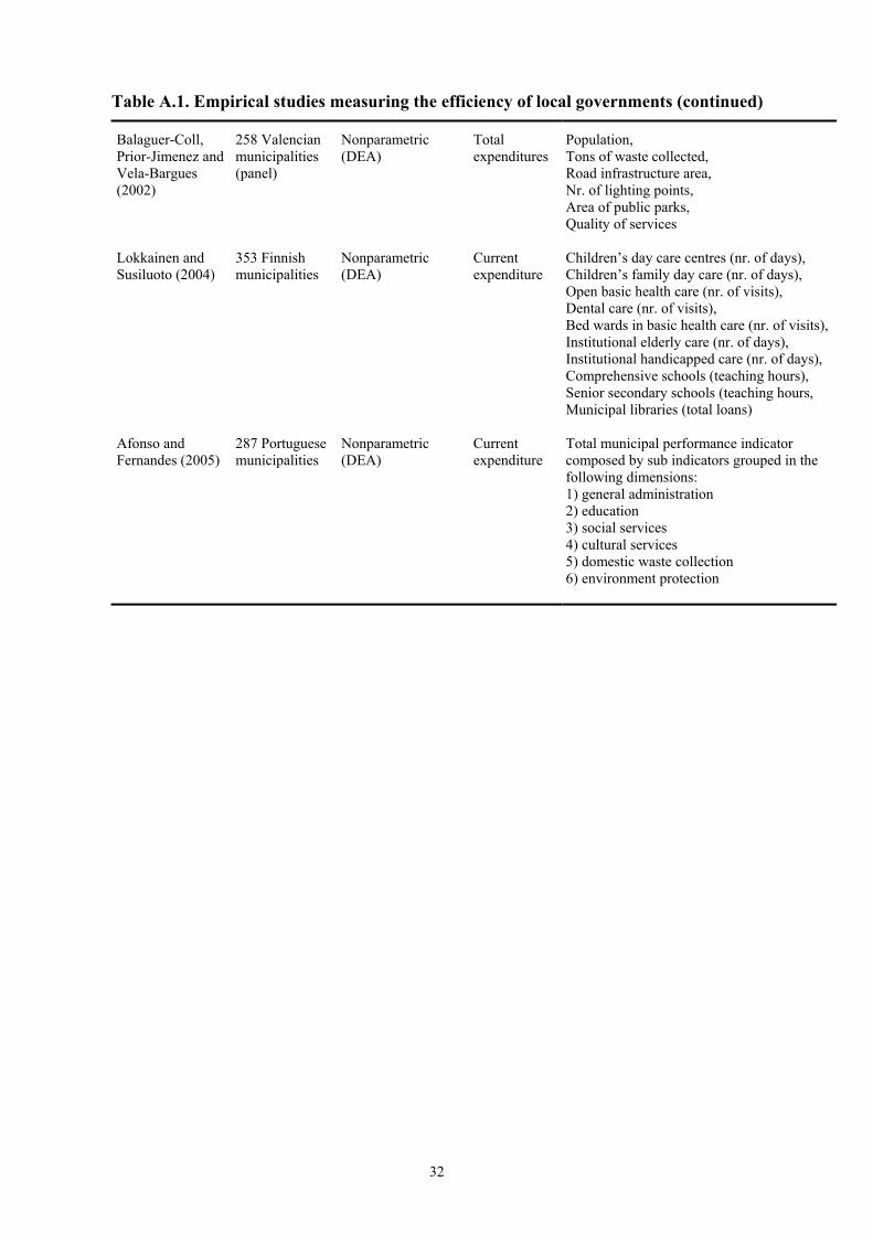
Mancebón, 2002), or water services (García-Sánchez, 2006). Table A.1 in the Appendix

provides a summary of the main features of these studies analysing ‘global’ efficiency

of municipal spending. All these works follow a rather consolidate scheme, made of

three successive steps:

1) first, one needs to choose indicators for inputs and outputs, and the methodology for

efficiency measurement;

2) second, an analysis of efficiency scores and their statistical distribution is

performed. In the case the researchers have used different techniques for measuring

efficiency, they also analyse the correlation between results obtained with different

methodologies;

3) finally, an investigation of the potential determinants of efficiency scores, generally

using a Tobit model is considered. Table A.2 in the Appendix summarise the main

results available in the literature on this point.

Because of its innovations and its accuracy, the study of De Borger and Kerstens (1996)

on Belgian municipalities represents the reference for all the following literature on

efficiency measurement in local governments. The authors were the first to use different

methodologies (following both approaches, parametric-SFA and nonparametric-DEA)

to measure the expenditure-efficiency of local governments. The use of more than one

methodology to measure efficiency stems from the attempt to check the robustness of

the results obtained through different measurement techniques. This example was

followed, e.g., by Worthington (2000) and Athanassopoulos and Triantis (1998), while

5

most of the authors preferred to avoid assuming a specific functional form for public

services provision, and to rely exclusively on nonparametric techniques only.

In the literature, the choice of input and output variables is strongly influenced by the

institutional framework under scrutiny. In particular, the output variables need to

represent the largest possible share of all the functions performed by local governments.

Therefore, according to the fundamental and juridical functions attributed to local

governments, we find more attention: on infrastructures’ maintenance and construction

in the Australian context; on educational and social services in Belgium and Finland; on

the efforts against poverty and illiteracy in Brazil; and on waste collection and territorial

planning respectively in Spain and Greece. On the contrary, given its feature to be more

comparable than other variables, almost every study individuates municipal current

expenditure as the only input consumed in the production of local services.

As for the determinants of efficiency, the literature explored the role of economic,

social, political, demographic, and geographic variables. Among all these, economic

variables appear to play the most important role. In particular, it is interesting to note

the role of grants and taxes. In all the studies, it appears that a high level of dependency

from central government transfers worsens the efficiency scores. As for taxation, results

are somewhat mixed. A positive relationship between high local tax rates and efficiency

scores emerges in Vanden Eeckaut et al. (1993) and De Borger and Kerstens (1996).

Hence, the impact on efficiency and – especially – on political control of public

spending depends on the main source of municipal revenue (taxes or grants). On the

contrary, in Balaguer-Coll et al. (2002), a high per capita level of tax revenues, as well

as of grants, has a negative influence on efficiency, because a larger availability of

public resources makes softer the budget constraint. These insights also characterize the

modern literature on fiscal federalism (e.g., Oates, 2005). The availability of more

revenues, both in the form of grants and local taxes, reduces the awareness of local

politicians to control spending. However, besides this ‘size’ effect, also the composition

of revenues matters. In particular, a higher dependency ratio (that is, a higher share of

transfers from central government to finance local spending) creates room for the

opportunistic behaviour of local politicians, because of bailout expectations and soft

budget constraint problems.

Other variables frequently used as explicative factors for spending efficiency are the

average municipal income and the educational level. They have an opposite impact on

6

efficiency, respectively negative and positive, because of their different influence on

citizens’ awareness and interest in public spending. As for demographic and geographic

controls, authors find a positive effect of population density and a negative effect of

marginal location of municipalities on efficiency, both effects explained by the

difficulties in services provision. Finally, political variables are almost all relevant but

the political orientation of local administration. Indeed, while Vanden Eeckaut et al.

(1993) and Athanassopoulos and Triantis (1998) highlight a negative relationship

between spending efficiency and both the number of parties in the governing coalition

and the parties affiliated to the central government, De Borger and Kerstens (1996) find

that the political orientation of local government does not seem to have a clear impact.

3. Empirical strategy

3.1. Data and variables

Our sample is composed by 262 municipalities belonging to the Province of Turin. The

Province of Turin represents an interesting case study, since it is the Italian Province

with the highest number of local governments (315), thus ensuring a great variability in

the data. This variability is confirmed not only by looking at the demographical

dimension (the Province includes Moncenisio, with 48 inhabitants, and Turin, with over

900,000 residents), but also in terms of territorial morphology (more than 10% of

municipalities is situated over 1,000 metres of altitude), management of public services,

political and economic characteristics, etc. However, at least to some extent, this huge

heterogeneity introduces potential biases in our analysis, especially for the presence of

municipalities that produce different services in different situations: the biggest

municipalities and those located at a high altitude. Therefore, we have decided to

exclude Turin and other municipalities over 15,000 inhabitants from the sample,

because they are clearly not comparable along several dimensions (like the type of

services produced) with the other ones1. Moreover, we excluded the municipalities

1 For instance, the share of current expenditure in the four sectors considered in our analysis represents less than 80% of their current spending for largest municipalities. Notice that small municipalities are prevailing in the sample, with almost 60% having less than 2000 inhabitants. Furthermore, the upper bound of 15,000 inhabitants represents an important threshold also from the perspective of the Italian political framework, as it indicates the minimum number of inhabitants for a municipality to be subject to the second ballot in municipal elections.

7

located over 900 meters of altitude2, as they show too high levels of expenditures with

respect to other municipalities (on average, 1800 Euro against 560 Euro per capita),

given the fact that their provision of services is strongly influenced not only by the

morphology of their territory, but probably also by heavy tourist inflows.

Data we use in the empirical analysis were provided by different institutions and refer to

the year 2005. The most relevant information comes from the Budgets of Italian

municipalities published by the Ministry of the Interior (the so-called Certificati

Consuntivi). Other important data, especially for output variables, have been obtained

from the statistical services of Regione Piemonte and Provincia di Torino. The selection

of input and output variables is strongly influenced by the Italian institutional

framework. Specifically, we selected indicators by looking at the most fundamental

competencies, both for municipal budget and for citizens. In Italy, municipal current

expenditure is classified in 12 macro-functions.

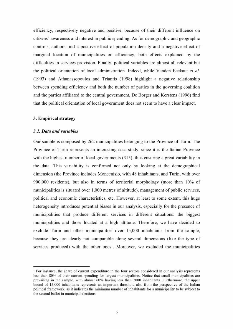
[FIGURE 1 HERE]

More than 90% of current expenditure in our sample is represented by five of these

macro-functions (see figure 1): General administration (39%); Territorial and

environmental management (22%); Educational services (13%); Child care, elderly care

and other social services (9%); Road maintenance and local mobility (8%). Clearly, the

share of these functions on local current expenditure varies according to the size of each

municipality: for instance, moving from the smallest municipalities (0-500 inhabitants)

to the biggest ones (between 10,000 and 15,000 inhabitants), the weight of general

administration decreases from 54% to 31%, while educational and social services

increase respectively from 6% and 5% to 13% and 12%. In our analysis, we use current

expenditures of municipalities (EXP) in each of these functions as input indicator. For

General administration, Educational services, Road maintenance and local mobility we

consider total expenditure as registered in the municipal budget. For Territorial and

environmental management and for Social services we just consider a fraction of total

expenditure. In fact, within Territorial and environmental management, Garbage

collection and disposal covers only a share, although relevant, of total expenditure

related to this function (60-70%). Therefore, we use only the expenditure dedicated to

this service, and not the entire function’s one, so as to improve the relationship with the 2 Dividing the municipalities according to their altitude, one can observe that just starting from 900 meters they show levels of average current spending beyond 1000 Euro per capita.

8

selected output indicator. Similarly, we separate from Social services’ total expenditure

the component specifically devoted to public welfare and elderly care. Our input

represents, on average, 86% of total current expenditure, with little variations across

different demographical classes of municipalities. Notice that this selection procedure

represents a significant improvement with respect to previous literature on local

governments’ efficiency, which has so far relied on a crude measure of current

expenditure considered as a whole.

We have then selected four output indicators directly connected with these expenditure

categories: the total population; the amounts of waste collected; the total length of

municipal roads; the number of people in needs of care (i.e. those under 14 years old –

enrolled in nursery, primary and secondary schools – and those over 75 years old). Even

if it is clearly not a direct output of local production, total population (POP) is assumed

to proxy for all the various administrative tasks Municipalities are involved in (e.g.,

maintaining the register of births, marriages, and deaths; issuing certificates, etc). The

number of people under 14 years old and over 75 year old (DEPEND) represents a

consistent fraction of the needy and it is strictly connected to educational and care

services. The amounts of waste collected (WASTE) is the direct result of the principal

competence in territorial and environmental management, i.e. garbage collection and

disposal. Total length of municipal roads (ROAD) is aimed at proxying especially the

competencies of municipalities in managing existing road infrastructures – i.e. road

maintenance, public lights, public transport arrangements, etc. – rather than in building

new roads (that belong to the capital expenditure category). This choice is in line with

the input variable as defined above. Table 1 shows the descriptive statistics for all

output and input indicators used in DEA and SFA models.

[TABLE 1 HERE]

It is worth noticing that our sample does not show input price variability. Indeed, there

is no wage flexibility as salary scales and allowances of municipal personnel are

completely fixed; moreover, all municipalities have access to the same capital market,

and obtain most of their funds from the same specialized financial institutions. Thus, the

hypothesis of identical input prices across municipalities is quite reasonable.3

Consequently, throughout the analysis we focus on the measurement of ‘global’ cost

3 About this issue, see also the discussion in De Borger and Kerstens (1996).

9

efficiency or, better, spending efficiency, as it is more closely related to the nature of

our data than pure technical efficiency.

3.2. Methodology

The techniques adopted to assess productive efficiency are usually classified in

parametric and nonparametric methods. We estimate here both a nonparametric

deterministic frontier (DEA) and a parametric stochastic frontier (SFA). Each

methodology actually presents advantages and flaws, but the literature has not been able

so far to establish when a technique is strictly superior to the other.

In parametric techniques, the functional form of the efficient frontier has to be defined a

priori, while in nonparametric techniques no functional form is pre-determined and only

basic properties of the production set are imposed as constraints to obtain the estimates.

On the other hand, SFA technique models both managerial inefficiencies and

uncontrollable factors (i.e., stochastic disturbances) that might impact on production

performances, while standard deterministic frontiers like DEA are able to account only

for inefficiency. Given these pros and cons, it is therefore important to check the

robustness of our results by using both approaches to investigate municipal spending

efficiency and its main determinants.

3.1. Data Envelopment Analysis

Data Envelopment Analysis, originating from Farrell (1957) seminal work and

popularised by Charnes et al. (1978), assumes the existence of a convex production

frontier. The production frontier in the DEA approach is constructed using linear

programming methods. The terminology ‘envelopment’ stems from the fact that the

production frontier really envelops the set of all observations.

The analytical description of the linear programming problem to be solved, in the

Variable Returns to Scale (VRS) hypothesis, is sketched below. Suppose there are k

inputs and m outputs for n DMUs. For the i-th DMU, qi is the column vector of the

outputs and xi is the column vector of the inputs. We can also define X as the (k×n)

input matrix and Q as the (m×n) output matrix. The DEA model is then specified as the

mathematical programming problem in (1), for a given i-th DMU:

10

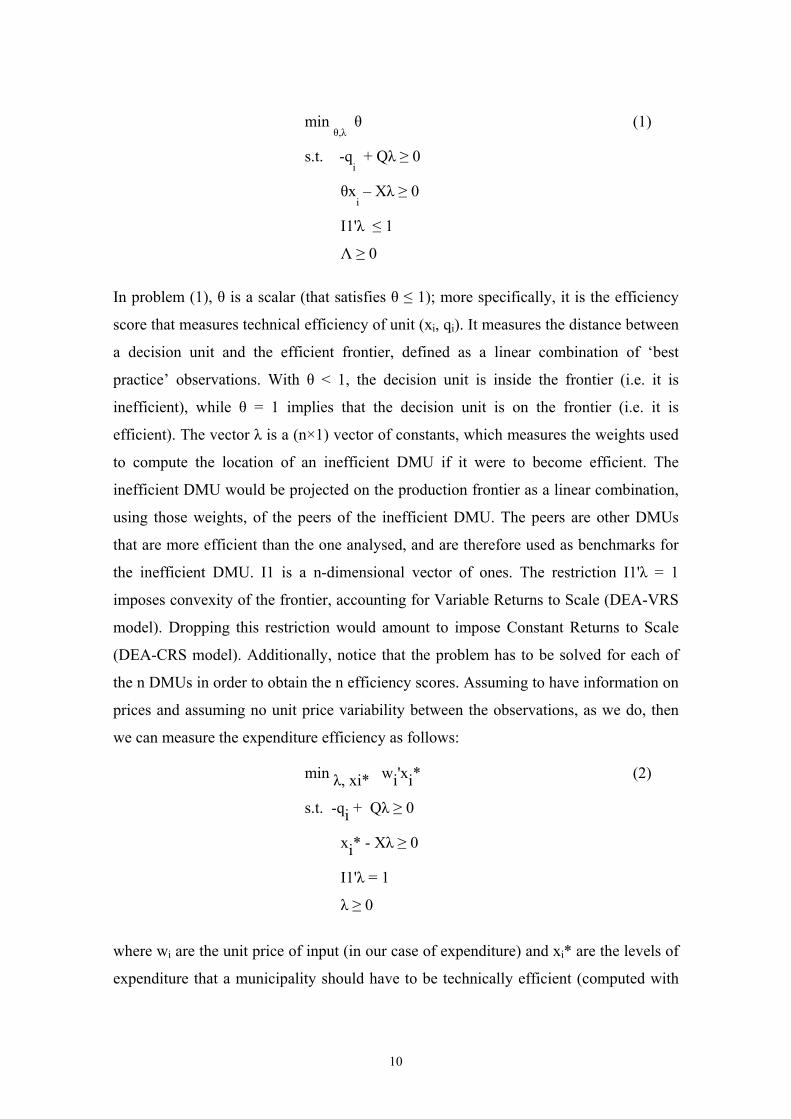
min

θ,λ θ

s.t. -qi + Qλ ≥ 0

θxi – Xλ ≥ 0

I1'λ ≤ 1

Λ ≥ 0

(1)

In problem (1), θ is a scalar (that satisfies θ ≤ 1); more specifically, it is the efficiency

score that measures technical efficiency of unit (xi, qi). It measures the distance between

a decision unit and the efficient frontier, defined as a linear combination of ‘best

practice’ observations. With θ < 1, the decision unit is inside the frontier (i.e. it is

inefficient), while θ = 1 implies that the decision unit is on the frontier (i.e. it is

efficient). The vector λ is a (n×1) vector of constants, which measures the weights used

to compute the location of an inefficient DMU if it were to become efficient. The

inefficient DMU would be projected on the production frontier as a linear combination,

using those weights, of the peers of the inefficient DMU. The peers are other DMUs

that are more efficient than the one analysed, and are therefore used as benchmarks for

the inefficient DMU. I1 is a n-dimensional vector of ones. The restriction I1'λ = 1

imposes convexity of the frontier, accounting for Variable Returns to Scale (DEA-VRS

model). Dropping this restriction would amount to impose Constant Returns to Scale

(DEA-CRS model). Additionally, notice that the problem has to be solved for each of

the n DMUs in order to obtain the n efficiency scores. Assuming to have information on

prices and assuming no unit price variability between the observations, as we do, then

we can measure the expenditure efficiency as follows:

min λ, xi* wi'xi*

s.t. -qi + Qλ ≥ 0

xi* - Xλ ≥ 0

I1'λ = 1

λ ≥ 0

(2)

where wi are the unit price of input (in our case of expenditure) and xi* are the levels of

expenditure that a municipality should have to be technically efficient (computed with

11

the previous DEA-VRS model). Then, it is possible to evaluate the allocative efficiency

component of total efficiency as the ratio between cost and technical efficiency.

2.2. Stochastic Frontier Analysis

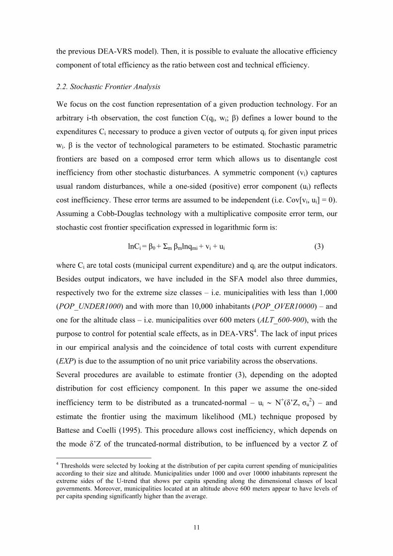
We focus on the cost function representation of a given production technology. For an

arbitrary i-th observation, the cost function C(qi, wi; β) defines a lower bound to the

expenditures Ci necessary to produce a given vector of outputs qi for given input prices

wi. β is the vector of technological parameters to be estimated. Stochastic parametric

frontiers are based on a composed error term which allows us to disentangle cost

inefficiency from other stochastic disturbances. A symmetric component (vi) captures

usual random disturbances, while a one-sided (positive) error component (ui) reflects

cost inefficiency. These error terms are assumed to be independent (i.e. Cov[vi, ui] = 0).

Assuming a Cobb-Douglas technology with a multiplicative composite error term, our

stochastic cost frontier specification expressed in logarithmic form is:

lnCi = β0 + Σm βmlnqmi + vi + ui (3)

where Ci are total costs (municipal current expenditure) and qi are the output indicators.

Besides output indicators, we have included in the SFA model also three dummies,

respectively two for the extreme size classes – i.e. municipalities with less than 1,000

(POP_UNDER1000) and with more than 10,000 inhabitants (POP_OVER10000) – and

one for the altitude class – i.e. municipalities over 600 meters (ALT_600-900), with the

purpose to control for potential scale effects, as in DEA-VRS4. The lack of input prices

in our empirical analysis and the coincidence of total costs with current expenditure

(EXP) is due to the assumption of no unit price variability across the observations.

Several procedures are available to estimate frontier (3), depending on the adopted

distribution for cost efficiency component. In this paper we assume the one-sided

inefficiency term to be distributed as a truncated-normal – ui ∼ N+(δ’Z, σu2) – and

estimate the frontier using the maximum likelihood (ML) technique proposed by

Battese and Coelli (1995). This procedure allows cost inefficiency, which depends on

the mode δ’Z of the truncated-normal distribution, to be influenced by a vector Z of

4 Thresholds were selected by looking at the distribution of per capita current spending of municipalities according to their size and altitude. Municipalities under 1000 and over 10000 inhabitants represent the extreme sides of the U-trend that shows per capita spending along the dimensional classes of local governments. Moreover, municipalities located at an altitude above 600 meters appear to have levels of per capita spending significantly higher than the average.

12

environmental observable factors. As for the symmetric random noise component vi, it

is assumed to be independently and identically distributed as a N(0, σv2).

Table 2 shows the estimates of equation (3) for our sample of 262 municipalities, using

EXP as dependent variable and the output indicators defined above and considering four

different SFA specifications (from Model 1 to Model 4) according to the set of selected

environmental variables.

[TABLE 2 HERE]

SFA estimates highlight the prevalence of inefficiency with respect to random noise in

determining global error term (ui + vi): γ – the share of total variance due to deviations

from the ‘best practice’ – varies from 0.687 in the SFA-Model 3 to 0.599 in the SFA-

Model 4. The municipality population (POP) and the amounts of waste collected

(WASTE) are particularly relevant in explaining the variability observed in current

expenditure levels. Moreover, constant returns to scale seem to dominate municipal

services provision, given the sum of estimated elasticities with respect to the four

outputs being very close to 1. This result depends crucially from the fact that 83% of

our observations do not belong to the two extremes of dimensional classes (i.e. under

500 and between 10,000 and 15,000 inhabitants, respectively). The importance of

demographical size and the altitude in defining cost frontier is also stressed by the

significant coefficients for the three dummies POP_UNDER1000, POP_OVER10000

and ALT_600-900, which point to the presence of some adverse scale impact on current

spending for the smallest and the biggest municipalities, as well as for the mountainous

and tourist ones.

4. Results

4.1. Comparing SFA and DEA inefficiency scores

We begin the discussion of our results with a classification of our municipalities based

on their size according to the number of inhabitants, that will help us in the analysis of

efficiency scores. Municipalities are divided in seven dimensional classes, following the

same classification introduced by the Ministry of Interior: under 499 inhabitants (13.5%

of observations), between 500 and 999 (22%), between 1,000 and 1,999 (25%), between

2,000 and 2,999 (9%), between 3,000 and 4,999 (15%), between 5,000 and 9,999

(11%), and finally over 10,000 (3.5%). We compare the results obtained from five

13

different models, one DEA-VRS and four SFA, where the last ones vary from the

poorest to the richest as for the included inefficiency determinants (i.e. the vector Z).

An elementary insight is obtained by considering the dichotomous classification of the

observations as either efficient or inefficient according to DEA evaluation (in SFA, by

construction, no observation is completely efficient): 22 municipalities – belonging

especially to the biggest and smallest dimensional classes (between 10,000 and 15,000

and under 500 inhabitants) – emerge as efficient units with a score equal to 1 (table 3).

[TABLE 3 HERE]

Considering both methodologies and all models, average inefficiency score is close to

0.22 for DEA-VRS and between 0.26 and 0.28 for SFA. It means that municipalities, on

average, could achieve the same output levels with about a 25% current spending

reduction. The scores distributions appear concentrated around the mean in both DEA

and SFA, since they exhibit a median close to the mean, and the 90% of observations

with less than 50% of spending inefficiency. Not surprisingly, standard deviation does

not show very high values, even if in SFA it is higher because of the presence of more

extreme score estimates.

[FIGURE 2 HERE]

The correlation between DEA and SFA inefficiency scores is very high both for VRS

and CRS specification. This means that the inclusion of the dummies for extreme

dimensions in stochastic cost frontier help to control for the effects of variable returns to

scale on efficiency estimates, like in DEA-VRS, even if they do not vanish completely.

Indeed, as previously discussed, SFA models highlight practically constant returns to

scale, like in DEA-CRS specification. Such a result is probably driven by the prevalence

in our sample of municipalities of small and medium sizes (82% of observations), for

which returns to scale appear to be constant looking at the difference between DEA-

CRS and DEA-VRS (see figure 2). Variable returns to scale appear instead to

characterise municipalities under 1,000 and between 10,000 and 15,000 inhabitants. The

first ones show increasing returns to scale, perhaps because of the influence of fixed

costs on current expenditures, that are very large for several services (e.g., waste

collection, general administration). The second ones mainly exhibit decreasing returns

to scale, probably as they produce a wider range of more complex services; this is

particularly true for elderly care and welfare spending (10% of current expenditures),

14

that include different social assistance items. Notice that the adopted variable DEPEND

is probably unable to fully capture the output results to be matched with the expenditure

devoted to this category. As for the best dimensional scale for providing the essential

public services considered in this study, the municipalities between 2,000 and 5,000

inhabitants seem to correspond to the optimal size; this evidence emerges by looking at

both the difference between DEA-CRS and DEA-VRS scores and SFA inefficiency

estimates (see figure 2).

As a final remark, in DEA-VRS model spending inefficiency (net of scale inefficiency)

seems to decrease with municipal size. This probably means that public managers are

subjected to a more severe control from their citizens when the latter can ask for

differentiated and more effective services. To explore this issue more in depth, we turn

now our attention to the possible determinants of estimated inefficiency.

4.2. Fiscal decentralization and other inefficiency determinants

We study the effects of fiscal decentralization and other possible explicative factors for

estimated inefficiency by adopting two different approaches. For DEA-VRS spending

model we use a standard two-stage analysis. Therefore, we take DEA-VRS inefficiency

scores and regress them on a set Z of environmental variables. We rely on a second-

stage Tobit regression, a censored model that permits us to make a proper inference on

the factors underlying inefficiency scores, considering also the presence of fully

efficient units. This choice is fundamental especially when using DEA, as the frontier

includes efficient observations with scores that take value 1. As for SFA spending

models, we adopt instead the single-stage estimation procedure proposed by Battese and

Coelli (1995, BC95 from now on): explanatory variables for inefficiency levels are

introduced directly in SFA equation (3) through a parametric specification of the error

term ui. Besides a measure of fiscal decentralization – the key issue of this study – the

other environmental variables included in both the Tobit and BC95 specifications

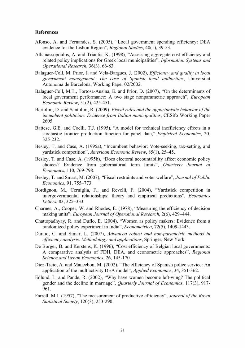
embrace a variety of economic, political and institutional factors. Descriptive statistics

for all the potential determinants of spending inefficiency are shown in table 4.

[TABLE 4 HERE]

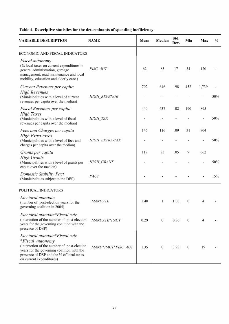
Tables 5 and 6 present the results for the determinants of spending inefficiency obtained

using SFA (BC95 model) and DEA-VRS (Tobit model) scores, respectively. We

15

estimated four different models for each group of scores, by augmenting the basic

specification (Model 1) with a richer set of explanatory variables (from Model 2 to

Model 4). All the estimates are extremely similar in terms of both the statistical

significance and the signs of coefficients, suggesting that our results are robust to

alternative model specifications.

In both set of estimates, the index of fiscal decentralization appears to have an

important influence on spending inefficiency. Similarly to other countries, Italian

municipalities rely on three main different sources of revenues: local taxes, central

government grants, and fees and charges. We define fiscal autonomy (FISC_AUT) as

the percentage of current expenditures (in the selected five functions) covered by local

taxes. Notice that it is the first time that such an indicator of fiscal decentralization is

used as explanatory variable for spending inefficiency. It appears that a municipality

with a higher share of current revenues derived from local taxes is more efficient, giving

support to the theoretical insight that a higher accountability of local politicians can be

obtained by increasing their responsibilities in terms of funding.

[TABLES 5 AND 6 HERE]

The impact of local taxes on municipal efficiency confirms previous findings in the

literature, and suggest that the other sources of revenues act in the opposite direction.

De Borger and Kerstens (1996) – using the local tax rates to proxy for fiscal autonomy

– refer to the ‘flypaper-effect’ to explain this relationship. Taxpayers are not able to

know the real entity of local government’s budget constraint, when the degree of fiscal

imbalance is high (Oates, 1999); in other words, citizens find more difficult to know the

level of grants rather than that of taxes. Therefore, it is easier for local politicians to turn

aside taxpayers’ attention from their inefficient behaviour, providing more expenditure,

just as the flypaper with the flies. Oates (1999) suggests also that transfers increase

public spending more than an equally increase of citizens’ income would increase their

purchase. Therefore, the share of current expenditures covered by local taxes appears to

have a positive effect on efficiency since local politicians are made more accountable,

given the tighter control exerted by the citizens-taxpayers. Local representatives, in fact,

use less easily local taxation than transfers and charges, as citizens are more aware of it.

In a similar vein, Silkman and Young (1982) underline another important aspect linked

to the relationship between fiscal autonomy and spending efficiency. In their opinion,

16

an inefficient behaviour of municipalities has a price, that is shared with other levels of

government according with the volume of funds that local governments receive from

them. In this case, local politicians can attribute bad management performance to

superior governments. Hence, a more precise definition of responsibilities for local

governments, not only from spending side but also from revenue side, should increase

spending efficiency.

Finally, our evidence is also in accordance with the predictions provided by electoral

accountability models, which the second-generation theory of fiscal federalism relies on

(e.g., Besley and Case, 1995a, Besley and Smart, 2007, Bordignon et al., 2004, Hindriks

and Lockwood, 2008). According to this framework, the presence of asymmetric

information between electorates (the principals) and politicians (the agents) can be seen

as the main reason why the government’s performance is inefficient. The crucial point

here is that fiscal decentralization can create an incentive to reduce rent diversion and/or

the influence of lobbies, leading to a higher probability of re-election of incumbent

politicians through mechanisms of tax competition and yardstick competition among

local governments.

The dummy HIGH_REVENUE is another fiscal variable showing a significant impact

on inefficiency in all estimates. It is equal to 1 for the municipalities with a per capita

level of current revenues over the median (over 646 Euro per capita)5. The first three

models using both SFA and DEA scores show a positive influence of this variable on

spending inefficiency. However, before interpreting this result in the light of the

literature on soft budget constraint and fiscal bailout problems in decentralized settings

(e.g., Prud’Homme, 1995, McLure, 1967, Inman, 2003), it is important to observe the

results obtained with Model 4. In this specification, municipal per capita current

revenues have been decomposed into their three principal sources: taxes (HIGH_TAX),

fees and charges (HIGH_EXTRA-TAX), and grants (HIGH_GRANT). Like for total

revenues, for each source we individuated municipalities characterised by a per capita

level exceeding the median6. Contrary to most of previous literature, our findings show

that the significant and positive effect of higher current revenues on inefficiency is not

due to a stronger incidence of grants, but of taxes as well as fees and charges. This

5 We use this kind of indicator because the distribution of per capita current revenues exhibit a particular variability: the values under the median are rather close (between 477 and 646 Euro per capita), while over the median they jump from 646 to 1,739 Euro per capita. 6 See previous footnote.

17

confirms the evidence emerged in Balaguer-Coll et al. (2002, 2007): a local government

that is highly capable of generating own revenues would be less motivated to manage

them efficiently. This insight also comes from property rights and principal-agent

literature, that outlines several reasons why politicians and public managers may lack

proper incentives to effectively audit and control expenditures. Moreover, the relevant

result for taxes and fees and charges is justified by the nature of our sample, where the

average weight of the central and regional transfers on the local current revenues is very

low (16%) with respect to the national mean (25%)7. Overall, these findings, linked to

the previous one on the impact of fical decentralization, highlight that, while more

autonomous municipalities tend to exhibit less inefficient spending behaviours, an

excessively large disposability of public resources – in particular, from taxes and fees

and charges – seems to exert a negative influence on spending efficiency, as it makes

softer the budget constraint for local governors.

The importance of the budget constraint faced by the municipalities is also investigated

directly trough the dummy variable PACT, that distinguishes local governments subject

to the Domestic Stability Pact (DSP) from the other ones. The DSP is a set of fiscal

rules that was introduced in Italy since 1999, as a consequence of the Stability and

Growth Pact (Amsterdam Treaty, 1997), to limit local administrations’ expenditures.

Fiscal rules usually consist in a limitation to the budget deficit and/or a direct limit to

the spending growth rate. The scope of the law spans over all levels of the Italian

territorial administrative structure: regions, provinces and municipalities. However,

starting from 2001, municipalities with less than 5,000 inhabitants were excluded from

the DSP. From our analysis, the presence of the DSP appears to have a significant and

reducing effect on spending inefficiency, even if only for DEA-VRS models (table 6),

probably because in SFA models this factor partly captures a size effect. Thus, the

imposition of a tighter budget constraint should reduce the opportunistic behaviour of

incumbent politicians and improve spending efficiency.

We now focus on some political features of municipalities. Both DEA-VRS and SFA

estimates in Model 1, 2 and 4 show that electoral mandate has a significant and positive

influence on spending inefficiency. The variable MANDATE assumes 5 different values

(from 0 to 4) and represents the number of post-election years for the mayor and the

7 See IRES Piemonte, Osservatorio sulla Finanza Locale del Piemonte, and Ministero dell’Interno, Dati sui Certificati di Bilancio dei Comuni.

18

governing coalition. This result is linked to previously quoted literature on political

accountability and in line with the electoral budget cycle approach. According to this

theoretical strand, incumbent politicians tend to enlarge spending in proximity of new

elections in order to increase their chances to be re-elected. (e.g., Rogoff, 1990, Besley

and Case, 1995b). Our empirical analysis seems to provide a clear evidence of the

electoral budget cycle effect, as the shorter is the distance from new elections year the

larger is the deviation from the best-practice frontier.

In Model 3, we have tested another landmark of the literature on the opportunistic

behaviour of incumbent politicians based on their desire to be re-elected. Interacting the

variable MANDATE with the variable PACT, we find that MANDATE*PACT impacts

on spending inefficiency in a significant and positive way, while the pure effect

associated to the number of post-election years loses its statistical significance. To

summarize, as in the recent contributions by Mink and De Haan (2005) and Bartolini

and Santolini (2009), there is evidence of an electoral budget cycle effect: spending

inefficiency increases in proximity of the election year, and the DSP seems quite

effective in controlling the budget of local administrations; however, the introduction of

such a fiscal rule (DSP) tend to strengthen remarkably the opportunistic behaviour for

those incumbent politicians that are closer to the end of their electoral mandate. We

finally add the variable MAND*PACT*FISC_AUT, that interacts the above term with

fiscal autonomy indicator; one can notice that a higher degree of fiscal decentralization

seems to reduce the electoral budget cycle impact, even though exisiting literature

signals decentralized setting as an incentive for incumbents’ opportunistic behaviours

related in particular to yardstick competition (Salmon, 1987; Besley and Case, 1995b).

We tried to control for possible relationships between the political orientation of

governing coalition and inefficiency scores, using two dummy variables that assume

value 1 if coalition parties belong to a civic list (CIV_LIST) or to a centre-left list

(CEN_LEFT). As for CEN_LEFT, it emerges a significant and reducing impact on

inefficiency in several specifications (BC95 Models 1, 2, 4 and Tobit Models 1, 2),

while the coefficient for CIV_LIST appears significant only in BC95 Model 4. These

results, however, are strongly influenced by a net prevalence in the sample of

municipalities led by civic lists (172 observations), all concentrated in small-sized local

governments. Notice that the positive effect on spending efficiency of centre-left

leading coalition is somewhat in contrast with political economy literature, that often

19

found in such a political orientation a propensity towards larger size governments (e.g.,

Edlund and Pande, 2002). Starting from Model 2 we have also included two variables

pertaining to the age (AGE_MAYOR) and to the gender of the mayor (SEX_MAYOR).

Both variables do not appear to affect significantly inefficiency, contrary to the bulk of

the literature on the size and the composition of public expenditure, that – especially for

female representatives – stresses their key role in determining policy preferences and

spending outcomes (e.g., Lott and Kenny, 1999; Edlund and Pande, 2002; Funk and

Gathmann, 2008; Pande, 2003; Chattopadhyay and Duflo, 2004; Svaleyrd, 2007; Geys

and Revelli, 2009).

Finally, we use three dummies for capturing the different management models of waste

collection and disposal that are observed in our sample. The choice to consider this

particular service is enforced by the presence of several governance structures, and

especially by the importance that the service has recently gained in Italy for judging a

local administration to be good (think for example to the scandals of Naples and

Palermo). This type of public service can be managed: a) directly by a local

government; directly by a consortium of local governments with the possibility for a

municipality to be b) either consortium head or c) a simple participant; through a single

firm which can be either d) public or e) private; through f ) a public cooperative firm

involving more than one municipality. We summarize these six different governance

schemes in three variables. A first dummy distinguishes the public ownership from the

private one (PUBLIC), a second dummy indicates a firm management conditional to

have public ownership (PUBLIC*FIRM), while a third dummy represents a cooperative

management conditional to be a publicly-owned firm (PUBLIC*FIRM*COOP).

The results we have obtained – both for BC95 and Tobit models – highlight a

significant effect of waste management type only for the latter dummy: they show that it

is neither important that the ownership of this local service is public or private, nor that

the provision is through a firm or directly from the municipality; it is, instead, relevant

that, besides being public and run through a firm, garbage collection and disposal is

managed cooperatively. The scheme of a publicly-owned cooperative firm would then

represent a more efficient solution, probably as it associates the advantage of solving

fixed costs problem (typical of consortium option) with the benefit of increasing

expenditure control (typical of external firm option). Indeed, within an external firm,

resource availability is lower, and then public managers are more aware of their

20

behaviours. Moreover, a consortium among different municipalities allows them to

share huge fixed costs.

5. Conclusions

The purpose of this paper is to assess spending efficiency for Italian municipalities,

investigating, in particular, the role played by a set of variables reflecting the degree of

fiscal autonomy. The analysis relies on a sample of 262 municipalities belonging to the

Province of Turin, and exploits both nonparametric (DEA) and parametric (SFA)

frontier techniques to study efficiency performances and their main determinants.

Consistently with fiscal federalism theories and the available empirical literature on

efficiency of local governments, our results suggest that more autonomous municipalities

exhibit less inefficient spending behaviours. Moreover, the strictness of budget

constraint due to the presence of some fiscal rules (here the Domestic Stability Pact)

appears to be important in driving efficiency. Finally, the importance of political

accountability highlighted by electoral budget cycle theories is confirmed empirically.

As for the political features of government coalition, both age and gender of the mayor

do not seem to exert any significant impact on inefficiency levels, while the political

ideology belonging to the left-wings tends to reduce excess spending.

From a policy perspective, the evidence emerged in this study provides support to

recent legislative reforms that aim at increasing fiscal autonomy of local governments,

in order to improve both the efficiency and the effectiveness of public services provided

to the citizens.

21

References

Afonso, A. and Fernandes, S. (2005), “Local government spending efficiency: DEA evidence for the Lisbon Region”, Regional Studies, 40(1), 39-53.

Athanassopoulos, A. and Triantis, K. (1998), “Assessing aggregate cost efficiency and related policy implications for Greek local municipalities”, Information Systems and Operational Research, 36(3), 66-83.

Balaguer-Coll, M. Prior, J. and Vela-Bargues, J. (2002), Efficiency and quality in local government management. The case of Spanish local authorities, Universitat Autonoma de Barcelona, Working Paper 02/2002.

Balaguer-Coll, M.T., Tortosa-Ausina, E. and Prior, D. (2007), “On the determinants of local government performance: A two stage nonparametric approach”, European Economic Review, 51(2), 425-451.

Bartolini, D. and Santolini, R. (2009). Fiscal rules and the opportunistic behavior of the incumbent politician: Evidence from Italian municipalities, CESifo Working Paper 2605.

Battese, G.E. and Coelli, T.J. (1995), “A model for technical inefficiency effects in a stochastic frontier production function for panel data,” Empirical Economics, 20, 325-232.

Besley, T. and Case, A. (1995a), “Incumbent behavior: Vote-seeking, tax-setting, and yardstick competition”, American Economic Review, 85(1), 25–45.

Besley, T. and Case, A. (1995b), “Does electoral accountability affect economic policy choices? Evidence from gubernatorial term limits”, Quarterly Journal of Economics, 110, 769-798.

Besley, T. and Smart, M. (2007), “Fiscal restraints and voter welfare”, Journal of Public Economics, 91, 755–773.

Bordignon, M., Cerniglia, F., and Revelli, F. (2004), “Yardstick competition in intergovernmental relationships: theory and empirical predictions”, Economics Letters, 83, 325–333.

Charnes, A., Cooper, W. and Rhodes, E. (1978), “Measuring the efficiency of decision making units”, European Journal of Operational Research, 2(6), 429–444.

Chattopadhyay, R. and Duflo, E. (2004), “Women as policy makers: Evidence from a randomized policy experiment in India”, Econometrica, 72(5), 1409-1443.

Daraio, C. and Simar, L. (2007), Advanced robust and non-parametric methods in efficiency analysis. Methodology and applications, Springer, New York.

De Borger, B. and Kerstens, K. (1996), “Cost efficiency of Belgian local governments: A comparative analysis of FDH, DEA, and econometric approaches”, Regional Science and Urban Economics, 26, 145-170.

Diez-Ticio, A. and Mancebon, M. (2002), “The efficiency of Spanish police service: An application of the multiactivity DEA model”, Applied Economics, 34, 351-362.

Edlund, L. and Pande, R. (2002), “Why have women become left-wing? The political gender and the decline in marriage”, Quarterly Journal of Economics, 117(3), 917-961.

Farrell, M.J. (1957), “The measurement of productive efficiency”, Journal of the Royal Statistical Society, 120(3), 253-290.

22

Funk, P. and Gathmann, C. (2008), Gender gaps in policy making: Evidence from direct democracy in Switzerland, Universitat Pompeu Fabra, mimeo.

García-Sánchez, I. (2006), “Efficiency measurement in Spanish local government: The case of municipal water services”, Review of Policy Research, 23(2), 355-371.

Geys, B. and Revelli, F. (2009), Decentralization, competition and the local tax mix: Evidence from Flanders, Department of Economics «S. Cognetti de Martiis» University of Torino, Working Paper 2/2009.

Hindriks, J. and Lockwood, B. (2008), Decentralisation and electoral accountability: Incentives, separation and vote welfare, mimeo.

Inman, R. P. (2003). “Transfers and bailouts: Enforcing local fiscal discipline with lessons from U.S. federalism,” in J. Rodden et al. (eds.), Fiscal decentralization and the challenge of hard budget constraints, Cambridge, MA, MIT Press, pp. 35–83.

Lokkainen, H. and Susiluoto, I. (2004), “Cost efficiency of Finnish municipalities 1994-2002. An application of DEA and Tobit methods”, paper presented at the 44th Congress of the European Regional Science Association, Porto, Portugal, 25-29 August 2004.

Lott, J.R. and Kenny, L.W. (1999), “Did women’s suffrage influences the size and scope of government?”, Journal of Political Economy, 107: 1163-1198.

McLure, C.E. (1967). “The interstate exporting of State and Local taxes: Estimates for 1962,” National Tax Journal, 20, 49-77.

Ministero dell’Interno, Dati sui certificati di bilancio dei Comuni, http://www.interno.it. Mink, M. and De Haan, J. (2005), Has the stability and growth pact impeded political

budget cycles in the European Union?, CESifo Working Paper 1535. Navarro, A. and Ortiz, D. (2003), “Propuesta metodológica para la aplicación del

Benchmarking a través de indicadores: una investigación empírica en administraciones locales”, Revista de Contabilidad, 6(12), 109-138.

Nordhaus, W. D. (1975). “The political business cycle”. Review of Economic Studies, 42(2), 169{190.

Oates, W.E. (1999), “An essay on fiscal federalism”, Journal of Economic Literature, 37(3), 1120-1149.

Oates, W.E. (2005), “Toward a second-generation theory of fiscal federalism”, International Tax and Public Finance, 12, 349-373.

Pande, R. (2003), “Can mandated political representation increase policy influence for disadvantaged minorities: Theory and evidence from India”, American Economic Review, 93(4): 1132-1151.

Prieto, A.M. and Zofio, J.L. (2001), “Evaluating effectiveness in public provision of infrastructure and equipment: the case of Spanish municipalities”, Journal of Productivity Analysis, 15, 41-58.

Prud’Homme, R. (1995), “The dangers of decentralization”, World Bank Research Observer, 10, 201-220.

Rogoff, K. (1990), “Equilibrium political budget cycles”, American Economic Review, 80, 21-36.

Salmon, P. (1987), “Decentralisation as an incentive scheme”, Oxford Review of Economic Policy, 3(2), 24-43.

23

Silkman, R. and Young, D.R. (1982), “X-Efficiency and state formula grants”, National Tax Journal, 35.

Simar, L. and Wilson, P.W. (2007), “Estimation and inference in two stage semi-parametric models of productive efficiency”, Journal of Econometrics, 136, 31-64.

Sousa, M. and Ramos, F. (1999). “Eficiencia técnica e retornos de escala na producao de servicos publicos municipais: O caso do nordeste e do sudeste brasileiros”, Revista Brasileira de Economia, 53(4), 433-461.

Svaleyrd, H. (2007), “Female representation: Is it important for policy decisions?”, paper presented at the 1st World Public Choice Conference, April 2007, Amsterdam.

Tiebout, C. (1956), “A pure theory of local expenditures”, Journal of Political Economy, 64(5), 416-424.

Tulkens, H., and Vanden Eeckhaut, P. (1995), “Nonparametric efficiency, progress and regress measures for panel data: Methodological aspects”, European Journal of Operational Research, 80, 474-499.

Vanden Eeckhaut, P., Tulkens, H. and Jamar., M.A. (1993), “Cost Efficiency in Belgian Municipalities”, in Fried H.O., Lovell C.A.K. and Schmidt S.S. (eds), The Measurement of Productive Efficiency. Techniques and Applications, Oxford University Press.

Worthington, A. (2000), “Cost efficiency in Australian local government: a comparative analysis of mathematical programming and econometric approaches”, Financial Accounting & Management, 16(3), 267- 424.

Worthington, A. and Dollery, B. (2001), “Measuring efficiency in local government: An analysis of New South Wales municipalities’ domestic waste management function”, Policy Studies Journal, 29(2), 232-249.

24

Figure 1. Macro-functions of municipal current expenditure in the Province of Turin

Territorial and environmental management

22%

Social Services9%

Economic development1%

Functions related to productive activities

0%

Justice0%

Local police5%

Tourism0%

Cultural services2%

Sports and entertainment

1%

Road maintanance and local mobility

8%

Educational services13%

General administration39%

Table 1. Descriptive statistics for output and input indicators of DEA and SFA spending models

VARIABLE DESCRIPTION NAME Mean Std. Dev. Min Max

OUTPUTS

Population (nr. of inhabitants) POP 2,657 2,826 102 13,835

Amounts of waste collected (quintals) WASTE 12,117 13,914 486 76,107

Total length of municipal roads (km) ROAD 33 28 3 240

Total number of pupils and old people (pupils enrolled in nursery, primary and secondary school + over 75 inhabitants)

DEPEND 466 488 16 2,449

INPUTS

Current expenditure (103 Euro) a) general administration b) garbage management c) road maintenance and local mobility d) education and elderly care

EXP 1,297 1,284 95 6,743

25

Table 2. Estimates of SFA spending model

*, **, *** statistically significant at the 1%, 5%, 10% respectively.

Table 3. Summary statistics for DEA and SFA inefficiency scores

Regressor C = EXP (Model 1)

C = EXP (Model 2)

C = EXP (Model 3)

C = EXP (Model 4)

ln POP 0.667*** (0.047)

0.653*** (0.048)

0.647*** (0.047)

0.697*** (0.044)

ln WASTE 0.195*** (0.030)

0.199*** (0.029)

0.203*** (0.029)

0.160*** (0.029)

ln ROAD 0.019* (0.011)

0.021* (0.013)

0.026** (0.011)

0.023** (0.010)

ln DEPEND 0.055* (0.032)

0.059* (0.032)

0.057* (0.032)

0.059** (0.029)

POP_UNDER1000 0.049* (0.026)

0.043 (0.026)

0.046* (0.026)

0.075*** (0.023)

POP_OVER10000 0.081** (0.040)

0.090** (0.042)

0.097** (0.041)

0.108*** (0.037)

ALT_600-900 0.052** (0.022)

0.055** (0.022)

0.054** (0.021)

0.038** (0.019)

σ2 (σu2 + σv2) 0.013***

(0.001) 0.013***

(0.001) 0.013***

(0.001) 0.010***

(0.001)

γ [σu2/(σu

2 + σv2)] 0.686*** (0.234)

0.680*** (0.259)

0.687*** (0.228)

0.599*** (0.187)

Nr. observations

Wald test [p-value]

262

6825.54 [0.000]

261

6762.53 [0.000]

261

6794.52 [0.000]

261

8631.28 [0.000]

DEA-VRS SFA-Model 1 SFA-Model 2 SFA-Model 3 SFA-Model 4

Mean 0.22 0.28 0.28 0.28 0.26

Standard deviation 0.12 0.17 0.17 0.17 0.17

Median 0.22 0.26 0.26 0.26 0.25

Max 0.52 0.90 0.88 0.87 0.97

Min 0.00 0.04 0.04 0.03 0.02

Nr. of fully efficient municipalities 22 - - - -

26

Figure 2. Distribution of DEA and SFA inefficiency scores by municipal size classes

27

Table 4. Descriptive statistics for the determinants of spending inefficiency

VARIABLE DESCRIPTION NAME Mean Median Std. Dev. Min Max %

ECONOMIC AND FISCAL INDICATORS

Fiscal autonomy (% local taxes on current expenditures in general administration, garbage management, road maintenance and local mobility, education and elderly care )

FISC_AUT 62 85 17 34 120 -

Current Revenues per capita 702 646 198 452 1,739 - High Revenues (Municipalities with a level of current revenues per capita over the median)

HIGH_REVENUE - - - - - 50%

Fiscal Revenues per capita 440 437 102 190 895 High Taxes (Municipalities with a level of fiscal revenues per capita over the median)

HIGH_TAX - - - - - 50%

Fees and Charges per capita 146 116 109 31 904 High Extra-taxes (Municipalities with a level of fees and charges per capita over the median)

HIGH_EXTRA-TAX - - - - - 50%

Grants per capita 117 85 105 9 662 High Grants (Municipalities with a level of grants per capita over the median)

HIGH_GRANT - - - - - 50%

Domestic Stability Pact (Municipalities subject to the DPS)

PACT - - - - - 15%

POLITICAL INDICATORS

Electoral mandate (number of post-election years for the governing coalition in 2005)

MANDATE 1.40 1 1.03 0 4 -

Electoral mandate*Fiscal rule (interaction of the number of post-election years for the governing coalition with the presence of DSP)

MANDATE*PACT 0.29 0 0.86 0 4 -

Electoral mandate*Fiscal rule *Fiscal autonomy (interaction of the number of post-election years for the governing coalition with the presence of DSP and the % of local taxes on current expenditures)

MAND*PACT*FISC_AUT 1.35 0 3.98 0 19 -

28

Table 4. Descriptive statistics for the determinants of spending inefficiency (continued)

VARIABLE DESCRIPTION NAME Mean Median Std. Dev. Min Max %

POLITICAL INDICATORS

Mayor’s gender (Municipalities with a male mayor)

SEX_MAYOR - - - - - 83%

Mayor’s age AGE_MAYOR 52 54 10 28 79 -

Civil list governing coalition CIV_LIST - - - - - 56%

Centre-left governing coalition CEN_LEFT - - - - - 23%

GARBAGE MANAG. INDICATORS

Public Management PUBLIC - - - - - 77%

Public Management by a firm PUBLIC*FIRM - - - - - 32%

Public Management by a coop. firm PUBLIC*FIRM*COOP - - - - - 27%

29

Table 5. Analysis of spending inefficiency determinants (BC95 estimates)

Regressor SFA scores

(BC95 Model 1) SFA scores

(BC95 Model 2) SFA scores

(BC95 Model 3) SFA scores

(BC95 Model 4)

FISC_AUT - 0.1946*** (0.0406)

- 0.1859*** (0.0406)

- 0.1673*** (0.0402)

- 0.4656*** (0.0510)

PACT 0.0006

(0.0362) - 0.0080 (0.0353)

- 0.0143 (0.0509)

0.0265 (0.0453)

CIV_LIST - 0.0143 (0.0219)

- 0.0135 (0.0215)

- 0.0125 (0.0213)

- 0.0354* (0.0201)

CEN_LEFT - 0.0471* (0.0258)

- 0.0479* (0.0251)

- 0.0400 (0.0249)

- 0.0492** (0.0228)

MANDATE 0.0155* (0.0104)

0.0185** (0.0081)

0.0147 (0.0089)

0.0137* (0.0079)

HIGH_ REVENUE 0.1755***

(0.0234) 0.1752***

(0.0224) 0.1763***

(0.0218) -

PUBLIC - 0.0112 (0.0161)

- 0.0255 (0.0201)

- 0.0236 (0.0198)

- 0.0194 (0.0177)

PUBLIC*FIRM 0.0127

(0.0369) 0.0119

(0.0363) 0.0103

(0.0355) 0.0321

(0.0307)

PUBLIC*FIRM*COOP - 0.0863**

(0.0527) - 0.0881**

(0.0385) - 0.0916**

(0.0382) - 0.0675**

(0.0325)

SEX_MAYOR - -0.0225 (0.0219)

-0.0215 (0.0215)

-0.0079 (0.0189)

AGE_MAYOR - -0.0457 (0.0403)

-0.0488 (0.0395)

-0.0096 (0.0355)

MANDATE*PACT - - 1.517*** (0.5564)

0.7291 (0.4758)

MAND*PACT* FISC_AUT - - - 0.3293*** (0.1220)

- 0.1634 (0.1045)

HIGH_TAX - - - 0.2268*** (0.0251)

HIGH_EXTRA-TAX - - - 0.0625*** (0.0159)

HIGH_GRANT - - - - 0.0121 (0.0223)

LR test

[p-value] 115.6

[0.000] 118.7

[0.000] 133.8

[0.000] 199.7

[0.000]

Log-likelihood 212.4 212.9 217.1 250.0

Nr. observations 262 261 261 261

*, **, *** statistically significant at the 1%, 5%, 10% respectively.

30

Table 6. Analysis of spending inefficiency determinants (Tobit estimates)

Regressor DEA-VRS scores (Tobit Model 1)

DEA-VRS scores (Tobit Model 2)

DEA-VRS scores (Tobit Model 3)

DEA-VRS scores (Tobit Model 4)

FISC_AUT - 0.0717*** (0.0267)

- 0.0675** (0.0269)

- 0.0529** (0.0265)

- 0.2177*** (0.0333)

PACT - 0.0826***

(0.0206) - 0.0821***

(0.0207) - 0.0952***

(0.0332) - 0.0702**

(0.0317)

CIV_LIST - 0.0134 (0.0166)

- 0.0127 (0.0166)

- 0.0118 (0.0163)

- 0.0162 (0.0156)

CEN_LEFT - 0.0317* (0.0189)

- 0.0330* (0.0189)

- 0.0277 (0.0187)

- 0.0256 (0.0177)

MANDATE 0.0118* (0.0063)

0.0137** (0.0065)

-0.0104 (0.0072)

0.0092* (0.0068)

HIGH_ REVENUE 0.0984***

(0.0133) 0.1003***

(0.0134) 0.1039***

(0.0132) -

PUBLIC - 0.0138 (0.0160)

- 0.0112 (0.0161)

- 0.0083 (0.0158)

- 0.0019 (0.0149)

PUBLIC*FIRM 0.0016

(0.0287) 0.0025

(0.0287) - 0.0054 (0.0281)

0.0075 (0.0264)

PUBLIC*FIRM*COOP - 0.0501*

(0.0296) - 0.0503*

(0.0296) - 0.0517*

(0.0291) - 0.0410 (0.0273)

SEX_MAYOR - 0.0011 (0.0169)

- 0.0009 (0.0166)

-0.0094 (0.0157)

AGE_MAYOR - -0.0384 (0.0307)

- 0.0488 (0.0395)

-0.0267 (0.0282)

MANDATE*PACT - - 1.5309*** (0.4145)

1.1025*** (0.3906)

MAND*PACT* FISC_AUT - - - 0.3326*** (0.0908)

- 0.2421*** (0.0856)

HIGH_TAX - - - 0.1170*** (0.0138)

HIGH_EXTRA-TAX - - - 0.0426*** (0.0127)

HIGH_GRANT - - - - 0.0159 (0.0155)

LR test

[p-value] 121.7

[0.000] 122.1

[0.000] 136.4

[0.000] 164.2

[0.000]

Log-likelihood 186.5 186.0 193.1 207.0

Nr. observations 262 261 261 261

*, **, *** statistically significant at the 1%, 5%, 10% respectively.

31

APPENDIX

Table A.1. Empirical studies measuring the efficiency of local governments

Authors Sample Methodology Input indicators

Output indicators

Vanden Eeckaut, Tulkens and Jamar (1993)

235 Belgian municipalities

Nonparametric (DEA)

Current expenditure

Population, Nr. of beneficiaries of minimal subsistence grants, Nr. of students enlisted in local primary schools, Public recreational facilities, Population older than 65, Nr. of local crimes

De Borger and Kerstens (1996)

589 Belgian municipalities

Nonparametric (DEA and FDH) and parametric (deterministic and stochastic frontier)

Current expenditure

Population, Nr. of beneficiaries of minimal subsistence grants, Nr. of students enlisted in local primary schools, Public recreational facilities, Population older than 65

Athanassopoulos and Triantis (1998)

172 Greek municipalities

Non parametric (DEA) and parametric (SFA)

Current expenditure

Nr. of resident families, Average residential area, Building area, Industrial area, Tourism area

Sousa and Ramos (1999)

1103 Brasilian municipalities

Non parametric (DEA)

Current expenditure

Population, Homes with clear water, Homes with solid waste collection, Illiterate population, Nr. of enrolled students in primary and secondary local schools

Worthington (2000)

177 municipalities of New South Wales (Australia)

Nonparametric (DEA) and parametric (SFA)

Nr. full-time workers, Financial expenditures, Other expenditures (materials)

Population, Nr. of properties acquired to provide the following services: potable water and domestic waste collection, Kilometers of sealed and unsealed roads (urban and rural)

Prieto and Zofio (2001)

209 municipalities from Castilla to Leon with less than 20000 inhabitants

Non parametric (DEA)

Budgetary expenditure

Population, Tons of waste collected, Road infrastructure area, Nr. of lighting points, Area of public parks, Potable water, Cultural and sportive infrastructure

32

Table A.1. Empirical studies measuring the efficiency of local governments (continued)

Balaguer-Coll, Prior-Jimenez and Vela-Bargues (2002)

258 Valencian municipalities (panel)

Nonparametric (DEA)

Total expenditures

Population, Tons of waste collected, Road infrastructure area, Nr. of lighting points, Area of public parks, Quality of services

Lokkainen and Susiluoto (2004)

353 Finnish municipalities

Nonparametric (DEA)

Current expenditure

Children’s day care centres (nr. of days), Children’s family day care (nr. of days), Open basic health care (nr. of visits), Dental care (nr. of visits), Bed wards in basic health care (nr. of visits), Institutional elderly care (nr. of days), Institutional handicapped care (nr. of days), Comprehensive schools (teaching hours), Senior secondary schools (teaching hours, Municipal libraries (total loans)

Afonso and Fernandes (2005)

287 Portuguese municipalities

Nonparametric (DEA)

Current expenditure

Total municipal performance indicator composed by sub indicators grouped in the following dimensions: 1) general administration 2) education 3) social services 4) cultural services 5) domestic waste collection 6) environment protection

33

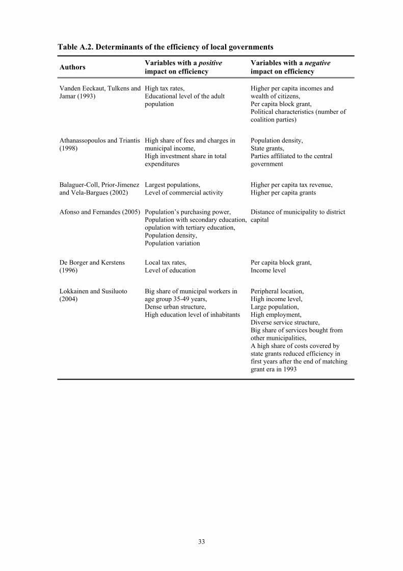
Table A.2. Determinants of the efficiency of local governments

Authors Variables with a positive impact on efficiency

Variables with a negative impact on efficiency

Vanden Eeckaut, Tulkens and Jamar (1993)

High tax rates, Educational level of the adult population

Higher per capita incomes and wealth of citizens, Per capita block grant, Political characteristics (number of coalition parties)

Athanassopoulos and Triantis (1998)

High share of fees and charges in municipal income, High investment share in total expenditures

Population density, State grants, Parties affiliated to the central government

Balaguer-Coll, Prior-Jimenez and Vela-Bargues (2002)

Largest populations, Level of commercial activity

Higher per capita tax revenue, Higher per capita grants

Afonso and Fernandes (2005) Population’s purchasing power, Population with secondary education,opulation with tertiary education, Population density, Population variation

Distance of municipality to district capital

De Borger and Kerstens (1996)

Local tax rates, Level of education

Per capita block grant, Income level

Lokkainen and Susiluoto (2004)

Big share of municipal workers in age group 35-49 years, Dense urban structure, High education level of inhabitants

Peripheral location, High income level, Large population, High employment, Diverse service structure, Big share of services bought from other municipalities, A high share of costs covered by state grants reduced efficiency in first years after the end of matching grant era in 1993