fiscal deficits and growth in developing countries · this paper examines the relation between...

Journal of Public Economics 89 (2005) 571–597

www.elsevier.com/locate/econbase

Fiscal deficits and growth in developing countries

Christopher S. Adam, David L. Bevan*

Department of Economics, University of Oxford, Manor Road, Oxford OX1 3UQ, United Kingdom

Received 16 December 2001; received in revised form 19 August 2003; accepted 12 February 2004

Available online 19 August 2004

Abstract

This paper examines the relation between fiscal deficits and growth for a panel of 45 developing

countries. Based on a consistent treatment of the government budget constraint, it finds evidence of a

threshold effect at a level of the deficit around 1.5% of GDP. While there appears to be a growth

payoff to reducing deficits to this level, this effect disappears or reverses itself for further fiscal

contraction. The magnitude of this payoff, but not its general character, necessarily depends on how

changes in the deficit are financed (through changes in borrowing or seigniorage) and on how the

change in the deficit is accommodated elsewhere in the budget. We also find evidence of interaction

effects between deficits and debt stocks, with high debt stocks exacerbating the adverse

consequences of high deficits.

D 2004 Elsevier B.V. All rights reserved.

JEL classification: H3; H6; O4

Keywords: Fiscal deficits; Growth; Threshold effects; Developing countries

1. Introduction

A great deal of attention has been devoted in both theoretical and empirical literatures

to the possible impact of various fiscal magnitudes on growth. In general, the theoretical

literature has been careful to respect the government budget constraint, which imposes the

requirement that a change in one magnitude has to be matched by offsetting changes

0047-2727/$ -

doi:10.1016/j.

* Corresp

E-mail ad

see front matter D 2004 Elsevier B.V. All rights reserved.

jpubeco.2004.02.006

onding author. Tel.: +44 1865 271075; fax: +44 1865 271094.

dress: [email protected] (D.L. Bevan).

C.S. Adam, D.L. Bevan / Journal of Public Economics 89 (2005) 571–597572

elsewhere. This has not usually been true of the empirical literature, which has frequently

examined the consequence of variations in a subset of budget items, implicitly assuming

that the (hidden) offsets elsewhere are growth neutral.1 Since the offsetting changes are

unspecified, and could take a variety of different forms, this assumption is strong—all

possible offsetting combinations are being treated as neutral. For example, consider the

common case where a study includes the share of government consumption expenditure in

GDP as one of the regressors, and interprets the coefficient on this variable as a measure of

the impact on the growth rate of a small increase in this share. This interpretation assumes

that the coefficient would be invariant to whether the increase was financed by a one-for-

one reduction in capital spending, or one-for-one increases in grant aid, tax revenue, or

deficit financing. Furthermore, it assumes that this neutrality would hold within each of

these categories, for example, between monetizing the deficit and increased public

borrowing.

Even in the theoretical literature, much of the effort has been devoted to consideration

of revenue neutral shifts in (more or less) distortionary taxes, and compositional shifts in

(more or less) productive expenditures in isolation, or to combinations of the two in a

balanced budget configuration. While there is also an extensive literature devoted to the

consequences of budget deficits, much of this has been in a context of lump sum taxation

and expenditure which is unproductive (as modelled, for example, by lump sum

transfers).2 Very little attention has been accorded to the fiscal issue of most practical

interest, where variations in distortionary taxes and/or productive expenditures may be

partly offset by changes in deficit financing.3

This paper examines this question in the context of developing countries. Most of the

existing empirical analyses in this area assume that the relation between deficits and

growth is linear.4 We show that while a linear representation tends to fit the data

reasonably well for our sample of developing countries, it nonetheless masks important

and policy-relevant non-linearities, especially at low levels of the fiscal deficit. In

particular, we show that for a sample of low- and middle-income countries, the

relationship is not linear: the gains to growth of fiscal contraction are most marked as

the deficit falls from a high level, but these taper out well before the economy reaches a

balanced budget position. Our empirical analysis suggests a statistically significant non-

linearity in the impact of the budget deficit on growth at around 1.5% of GDP. However,

this non-linearity reflects the underlying composition of deficit financing; a corresponding

threshold effect characterises the effect of seigniorage-financing on growth, but there is no

evidence from our data of a similar non-linearity arising from debt-financing.

1 For an extensive survey of the literature from this perspective, see Gemmell (2001).2 We here follow the common terminology for distinguishing between expenditure which enhances output—

is dproductiveT—and that which does not. dUnproductiveT expenditure may however be of high social value, for

example, by entering utility directly; hence it should not be confused with waste, though it might include that.

4 For example, Easterly et al. (1994), Miller and Russek (1997) and Kneller et al. (2000). One notable

exception is Giavazzi et al. (2000).

3 For example, in one of the leading textbooks on growth, Barro and Sala-I-Martin (1995), the discussion of

government and growth (pp. 152–161) presupposes a continuously balanced budget, so consideration of public

debt is excluded. In another, Aghion and Howitt (1998), government as a fiscal institution barely makes an

appearance; the only consideration of public debt is relegated to one of the problem sets. (Problem 7 of Chapter 1).

C.S. Adam, D.L. Bevan / Journal of Public Economics 89 (2005) 571–597 573

This type of non-linear relationship is quite plausible a priori. The distortionary impact

of taxation is increasing in the tax rate, while that of a very small deficit may be low. Hence,

for a given level of government spending, a shift from a balanced budget to a (small) deficit

may temporarily reduce distortions, depending on the composition of deficit financing.5 If

these distortions impact on growth rather than simply on output levels, it is therefore

feasible that growth will be maximised when there is some recourse to deficit financing.

The rest of the paper is organized as follows. Section 2 considers how deficit financing

might be considered in the context of distortionary taxes and productive expenditure. We

set up a simple overlapping generation model in the tradition of Diamond (1965) which

incorporates high-powered money in addition to debt and taxes. Section 3 describes the

empirical model and the estimation strategy, which allows for both threshold effects in the

deficit and its financing, and interactions between the deficit and debt stocks. Section 4

presents our econometric results based on data from the IMF’s Government Finance

Statistics for 45 developing countries over the period 1970–1999, and Section 5 concludes.

2. Deficit-financing when government operations are not neutral

2.1. The model

In our empirical application, we will be concerned with the impact on growth of both

deficit flows and debt stocks, both independently and interactively. Most of the data are

drawn from economies which are far from balanced growth or bsteady stateQ configurations.To motivate this empirical analysis, we therefore set up a simple Overlapping Generations

(OLG) model of savings behaviour which is then embedded in an endogenous growth

model along the lines of the model of government and growth due to Barro (1990) and

Barro and Sala-I-Martin (1992). We restrict our attention to a general flat-rate tax on output,

so that the possibility of shifts in the composition of taxes is ignored. The government

spending activity simply involves purchases of current output; there is no separate

production process. Government spending may either create a congestible productive

public good or it may enter (some) consumers’ utility directly, but have no consequences for

output.6 Our model differs from theirs in one crucial respect; the government budget need

not be balanced, and a deficit may be financed either by printing money and/or issuing

debt. Debt may be domestically or externally held; domestic debt carries an interest rate

equal to the net private rate of return. For the most part, we assume that external debt is

available on exogenous terms, including the case where a rationed amount of external debt

is available at an exogenously determined concessionary interest rate.7

5 The longer-run effects may be quite different, since the deficit will also raise the debt stock or inflation rate

over time, and that will in general also impact on growth.6 This dunproductiveT expenditure could be expenditure by those controlling the government in their own

interests, with no benefit to the general population, or expenditure which enters consumers’ utility functions

directly, but in a way that is neutral to their inter-temporal decisions. In both cases, the only impact it has on

growth is via the financing requirements it imposes.7 The model abstracts from real exchange rate issues, so there is no bsecondary burdenQ of external debt.


2.2. Individuals

Individuals live for two periods, inelastically supplying a unit of labour in the first, and

consuming in both. Population, and, equivalently, the labour force, grows at the constant

rate n. Given the structure of the model, this has no implications for the dynamics, but

means that the growth rate needs to be deflated by n to obtain per capita income growth.

There are no intergenerational transfers, and utility takes the additive logarithmic form:

U ¼ blnc1 þ 1� bð Þlnc2 ð1Þ

where c1, c2 are first- and second-period consumption and b is a preference parameter.8

2.3. Production

Since the empirical application is to countries with very different rates of population

growth, it is unappealing to model growth effects subject to a stationary population.

However, many endogenous growth models suffer from scale effects, where average and

marginal products of capital are proportional to the size of the workforce. The model

utilized here avoids that shortcoming, but this complicates the growth relations somewhat.

The productive public expenditure, denoted Gp, is here supposed to have benefits in

proportion to the aggregate labour force; i.e. it is congestible in the number of workers

over whom it is spread. There is also a positive externality associated with the overall

capital intensity of production in the economy. The representative firm’s production

function takes the Cobb Douglas form:9

yi ¼ Aaþbl1�ai ka

i K=Lð Þb Gp=L� �1�a�b ð2Þ

where the firm is indexed by i, and has constant returns in the factors it hires. li is firm i’s

labour force, and ki its capital stock. L is the aggregate labour force, and K the aggregate

capital stock. A is a productivity index, common across firms and constant over time.

Abstracting from depreciation, competitive markets then ensure that:

r ¼ 1� sð Þ@yi=@ki ¼ 1� sð ÞaAaþb ki=lið Þa�1K=Lð Þb Gp=L

� �1�a�b ð3Þ

where s denotes the flat-rate tax on output. Hence for the economy in aggregate, and

letting cp=Gp/Y,

Y ¼ AaþbKaþbG1�a�bp ¼ AKc 1�a�bð Þ= aþbð Þ

p ð4Þ

r ¼ 1� sð ÞaAc 1�a�bð Þ= aþbð Þp ð5Þ

8 This functional form has the convenient and, in the context of developing countries, not wholly unrealistic

consequence that saving is inelastic with respect to the interest rate. Specifically, if the net of tax wage is w, then

first period consumption is bw and saving is (1�b)w, and this holds whatever the combination of assets, structure

of returns, and anticipated tax rate.9 Time subscripts are omitted to simplify the notation where that does not risk confusion.


and the net-of-tax wage bill is:

W ¼ 1� sð Þ 1� að ÞY : ð6Þ

2.4. Government

All government activities are scaled relative to GDP (Y). The government makes two

kinds of expenditures, a productive type, as noted above, in relative amount cp=Gp/Y and

an unproductive type in amount cu. It receives grant aid in ratio to income of ae, and sets a

flat-rate output tax at rate s. Domestic debt is all short-term. The stock outstanding at the

start of period t is Ddt which is retired in the period and fresh one-period debt in the

amount Ddt+1 is floated. The interest rate on domestic debt in period t, rdt, is equal to the

net of tax return to capital, possible intermediated by an inflation effect (see below). The

end-of-period debt–income ratio is Ddt+1/Yt=Ddt+1, and the beginning of period ratio is

Ddt/Yt=(Ddt/Yt�1)(Yt�1/Yt)=Ddt/(1+gt). Similar relations hold for external debt, indexed

by e, except that re is exogenous.

The government also obtains financing from seigniorage, partly from real growth in the

economy, partly (perhaps) from inflation. This is in the amount Rt/Yt=rt. The

conventional deficit after grants and interest payments is therefore

dtYt ¼ Rt þ Ddtþ1 � Ddtð Þ þ Detþ1 � Detð Þ: ð7Þ

where dt is the ratio of this deficit to GDP in period t.

The government budget constraint, relative to GDP, is:

st ¼ cpt þ cut � aet þ rdtDdt þ retDet � dt ð8Þ

or, by substituting for the components of the deficit:

st ¼ cpt þ cut � aet � rt þ1þ rdtð Þ1þ gtð Þ Ddt � Ddtþ1

�þ 1þ retð Þ

1þ gtð Þ Det � Detþ1

�:

��

ð9Þ

2.5. Money

Money enters the model as an input into production, specifically the process of

capital accumulation, and into consumption, as part of the transactions technology. In

both cases, firms and households can economize on money so that their demand for real

balances is a function of the rate of inflation, which is assumed to be known with perfect

foresight. The full monetary mechanism is sketched in an Annex, bMoney in the OLG

ModelQ, which is available from the authors on request; here we present only its main

features.

The representative firm’s capital formation in period t requires capital goods and

working capital (real balances). Capital formation is financed from the savings of the

cohort who were young in t�1. Part of total savings is absorbed by the domestic

government bond issue, Ddt, with the balance represented by goods and real balances from

t�1. Net savings are then transformed into capital goods and working capital, the real


value of the latter being determined by the government’s choice of inflation (equivalently

its issue of high powered money). This generates the firm’s demand for money as:

mpt ¼ mp It;ptÞð ð10Þ

where It denotes the investible resources available to the firm, mIpN0, and mp

pb0. Inflation

therefore reduces the demand for real money balances and also drives a wedge between

investible funds and installed capital. High inflation means that a given quantum of

investible resources yields a lower amount of useable capital. Hence:

Kt=It ¼ u ptð Þ ¼ ut ð11Þ

which is monotonically decreasing in pt.10

The representative consumer’s demand for money is somewhat simpler consisting of a

standard cash in advance constraint of the form:

mct ¼ mc Wt; ptð Þ ð12Þ

where Wt is the net of tax wage bill, mWc N0, and mp

cb0. Combining these demands,

aggregate real balances are mt=mct+mpt. Government receives total seigniorage from these

combined balances of Rt=(1+pt)mt�mt�1. Expressed as a share of GDP, this is denoted

r=R/Y.

The monetary component of the model therefore incorporates a real seigniorage

mechanism where the government sets inflation (the growth of nominal high-powered

money) as a tax instrument, taking into account the impact on the tax base (real balances)

which is determined, in the light of inflation, by firms and consumers. Thus, on the one

hand, inflation generates additional seigniorage for government, lowering the distortionary

impact of tax financing. On the other hand, it itself induces a distortion, reducing the

efficiency with which investible resources are transformed into productive capital.11 The

monetary model is then spliced onto the real model previously outlined to derive an

expression for the growth rate of the economy in terms of the fiscal factors.

2.6. The growth rate

From Eq. (1), aggregate saving is simply:

St ¼ 1� bð ÞWt ¼ 1� bð Þ 1� að Þ 1� stð ÞYt;

and from Eq. (11):

Ktþ1 ¼ utþ1Itþ1 ¼ utþ1 St � Ddtþ1Þ:ð

10 Also, utV1 as p tz0. This specification means that the gross rate of return to saving only coincides with the

marginal product of capital when inflation is zero; the ratio between the two is also given by u t.11 It also reduces the efficiency with which produced goods are turned into consumption, and hence lowers

welfare. However, in the present context, this mechanism does not affect the growth rate. Notice also that inflation

lowers the rate of return to saving. Given the specification of utility, this does not alter the savings ratio.


Now the growth rate of output between periods t and t+1 is:

gtþ1 ¼Ytþ1

Yt� 1 ¼

AKtþ1c1�a�bð Þ= aþbð Þptþ1

Yt� 1:

Hence by substitution we obtain the growth equation:

gtþ1 ¼ Autþ1 1� bð Þ 1� að Þ 1� stð Þ � Ddtþ1

ic 1�a�bð Þ= aþbð Þptþ1 � 1

hð13Þ

which shows that growth between t and t+1 depends on the tax rate in t, the domestic debt

stock at the end of t, and the inflation rate and government productive spending in t+1.12

Eqs. (9) and (13) provide the basis for a partial analysis of the one-period growth effects

of various government policy changes to which we now turn.13

2.7. Trade-offs involving the tax rate

To illustrate the relevant properties of this model, we proceed by analysing the growth

consequences of a change in the tax rate offset by each of the other six budget components

in turn. Any other pair-wise combination can be inferred from this. Specifically, Eq. (13) is

differentiated with respect to the instrumental changes under consideration, and Eq. (9) is

differentiated to ensure that these changes respect budget balance.

(i) First, and most obviously, a tax-financed rise in unproductive expenditure is always

growth reducing, though it might still be welfare-enhancing if it entered individual utility

functions.

(ii) By the same token, increased grant aid is growth-enhancing if it is used to reduce

taxes, to lower domestic debt, or to increase productive spending. Its effect on growth is

neutral if it is used to finance non-productive expenditure.

(iii) A (sustained) rise in the tax rate to finance a (sustained) increase in productive

expenditure will be growth-enhancing if:

1� bð Þ 1� að Þ 1� stð Þ � cpta þ b

1� a � b

�NDdtþ1

�ð14Þ

This trade-off is intermediated by the level of domestic debt. The higher domestic debt

the lower the growth-enhancing levels of both taxation and productive expenditure.

(iv) The impact of reducing the output tax and financing the deficit by increased

seigniorage is less straightforward. Since the system is complex, we do not offer a full

discussion of its properties here. However, the outlines are clear enough. Raising the

inflation rate from a sufficiently low level does create additional seigniorage, permitting a

cut in taxes which enhances growth, but it is also directly inimical to growth. It is unclear,

a priori, which effect predominates. If the demand for money is essentially consumption-

12 Following Barro (1990), the provision of public services involves a call on resources at the same time as it

enhances output.13 The present model is a rich one, but a fuller exploration of its properties would take us too far afield in the

present context. To keep the discussion manageable, we will assume that if the expenditure ratio (cp) is changed inthe current period, it will be maintained at its new value in the following period. Hence there may be offsetting

effects on growth of financing increased spending.


driven (so that u is close to 1 and insensitive to inflation), then there is little growth impact

from inflation, and growth will be maximised if inflation is set close to the seigniorage

maximising level. On the other hand, if the demand for money is essentially production-

driven, there is likely to be a serious growth penalty associated with inflation.14

The effect on this trade-off of domestic debt is somewhat surprising. Total

differentiation of Eq. (13) with respect to the inflation rate yields:

dg ¼ Ac 1�a�bð Þ= aþbð Þp 1� bð Þ 1� að Þu 1� sð Þ � ds

1� sð Þ þ duu

� Dddu

��ð15Þ

The trade-off so far discussed is the term in the curly brackets. The inclusion of

domestic debt has two consequences. First, while, as already noted, its existence is

inimical to growth, it tends to make inflation-financing more likely to be attractive (since

dub0). Second, inflation has the effect of altering the interest cost of domestic public debt.

Specifically, rd ¼Aac 1�a�bð Þ= aþbð Þp u 1� sð Þ, so the impact of inflation on this rate also has

the sign of �ds1�sð Þ þ

duu

on. This second effect will therefore tend to offset the first, but will

be much weaker.

(v) The impact on growth of financing a tax cut by increasing domestic debt has the

sign of � 1� bð Þ 1� að Þdst � dDdtþ1 ¼ � 1� 1� bð Þ 1� að Þ½ �dDdtþ1 which is always

negative. This effect is linear in the deficit and invariant to the level of the debt stock,

though the latter does help determine the tax rate itself. Notice that domestic debt is

damaging even if rdbg. Whereas in the exogenous growth model it can be beneficial to

crowd out capital if the interest rate is very low, because the economy is dynamically

inefficient, this is never so in the endogenous growth case. Crowding out capital through

domestic debt is always costly, even if the higher debt ratio is more than self-financing.

(vi) External debt differs in two ways. First it does not have the direct crowding out

effect of domestic debt.15 Second, the interest rate will in general depend on some supply

curve of foreign savings.16 Here we assume that this rate is exogenous. There are two

cases to consider. In the first, reNg, and increased external debt sooner or later imposes a

net budgetary cost. Thus the impact effect on growth of using increased external finance to

permit a temporary tax cut is positive (dst=�Det+1); however, when the external debt

income ratio is stabilised at its new higher level, the tax rate must rise above its original

level (ds ¼ re�g

1þgdD), so the growth rate falls below its original level. In this case, growth is

positively associated with the deficit and negatively associated with the debt stock.

The second case is where external finance is available on concessionary terms, and

specifically rebg. Leaving aside the practically important issue of the likely finite horizon

for this concessionary window, we stress the other feature, that the supply is rationed at

any one time. Increased external debt now assists growth in the stock–income ratio as well

as the flow, and is analytically equivalent to changes in the aid flow, ae.

14 Simulations based on reasonable parameter values for the model presented in the annex referred to earlier

suggest that this cost may dominate any gains from the tax reduction permitted by the increased seigniorage.15 Of course, it may have an indirect effect if it discourages investment because of reduced confidence.16 If, instead, we followed Diamond in assuming that the interest rate on external debt equalled that on

domestic debt, it would always pay (in the endogenous growth model without real exchange rate or confidence

effects) to use additional external finance to retire domestic debt.


2.8. Summary

This discussion has posited two types of government spending, and five ways of

financing it, taxes, grants and three forms of deficit finance. It suggests that while the

impacts on growth of taxes and grants are reasonably straightforward, the impact of the

deficit is likely to be complex, depending on the financing mix and the outstanding debt

stock. In particular, deficits may be growth-enhancing if financed by limited seigniorage;

they are likely to be growth inhibiting if financed by domestic debt17; and to have opposite

flow and stock effects if financed by external loans at market rates.

3. Empirical model and estimation strategy

Our empirical results are based on the growth Eq. (13) and the representation of the

government budget constraint given by Eqs. (8) and (9). Before presenting our

econometric evidence, it is instructive to consider a simple scatter plot of our data. Fig.

1 plots average annual per capita income growth against the fiscal deficit after grants and

interest payments for 45 non-OECD countries for the period 1970–1999.18 This scatter is

overlaid with a semi-parametric estimate of the sample relationship between the two (see

Robinson, 1988). For convenience we have also plotted vertical lines corresponding to a

balanced budget, and deficits of 1.5% and 5% of GDP.

Given the high variance in the data, this evidence is only tentative but it does suggest

that while the dominant feature of the data is the negative correlation between fiscal

deficits and growth, there is also a hint that this effect may not be linear.19 To examine this

possibility in a more robust fashion, we proceed in three steps. First, we examine the role

of the deficit itself on growth, based on the budget constraint defined in Eq. (8) above.

Next, in line with Eq. (9), we substitute the deficit for its financing. In both cases, we test

for and find important non-linearities in these relationships. Finally, we examine the stock–

flow interaction between the deficit and net public indebtedness. Our first growth

regression model is therefore of the form:

gyit ¼ bVXit þ xVWit þ hhit W1 � WW1

�itþ uit

hit ¼ 1 if W1NWW1

0 if W1VWW1

ð16Þ

and uit ¼ li þ kt þ eit:

19 The bivariate linear regression of growth on the fiscal deficit using these pooled data has the form

y=2.919�0.233x where the standard errors on the intercept and slope coefficients are 0.346 and 0.082,

respectively. The equation has an overall R2 of 0.047. Not surprisingly given the variance in the data, it is not

possible to statistically discriminate between these simple linear and non-parametric regressions.

17 The starkness of this result depends on the 100% crowding out property of the present model. In practice,

the role of domestic debt as a component in the liquidity of the financial system also suggests caution in relying

on the sharp difference between money and debt adopted here.18 Details of country coverage and data definitions are provided in Table 1 and Appendix A.

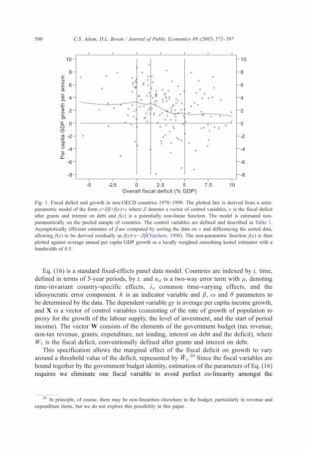
Fig. 1. Fiscal deficit and growth in non-OECD countries 1970–1999. The plotted line is derived from a semi-

parametric model of the form y=Zb+f(x)+e where Z denotes a vector of control variables, x is the fiscal deficit

after grants and interest on debt and f(x) is a potentially non-linear function. The model is estimated non-

parametrically on the pooled sample of countries. The control variables are defined and described in Table 1.

Asymptotically efficient estimates of b are computed by sorting the data on x and differencing the sorted data,

allowing f(x) to be derived residually as f(x)=y�Zb(Yatchew, 1998). The non-parametric function f(x) is then

plotted against average annual per capita GDP growth as a locally weighted smoothing kernel estimator with a

bandwidth of 0.5.


Eq. (16) is a standard fixed-effects panel data model. Countries are indexed by i, time,

defined in terms of 5-year periods, by t, and uit is a two-way error term with li denoting

time-invariant country-specific effects, kt common time-varying effects, and the

idiosyncratic error component. h is an indicator variable and b, x and h parameters to

be determined by the data. The dependent variable gy is average per capita income growth,

and X is a vector of control variables (consisting of the rate of growth of population to

proxy for the growth of the labour supply, the level of investment, and the start of period

income). The vector W consists of the elements of the government budget (tax revenue,

non-tax revenue, grants, expenditure, net lending, interest on debt and the deficit), where

W1 is the fiscal deficit, conventionally defined after grants and interest on debt.

This specification allows the marginal effect of the fiscal deficit on growth to vary

around a threshold value of the deficit, represented by W1.20 Since the fiscal variables are

bound together by the government budget identity, estimation of the parameters of Eq. (16)

requires we eliminate one fiscal variable to avoid perfect co-linearity amongst the

20 In principle, of course, there may be non-linearities elsewhere in the budget, particularly in revenue and

expenditure items, but we do not explore this possibility in this paper.


regressors. Defining the budget identity asPl

j¼0 Wj ¼ 0 and substituting out one of the

fiscal factors, denoted W0, Eq. (16) is re-written as:

gyit ¼ bVXit þXmj¼1

wjVWjit þ hhit W1 � WW 1

�itþ uit ð17Þ

where the coefficient wj=(xj�x0) now measures the marginal impact of fiscal factor Wj

on growth, net of the marginal impact of the excluded factor W0. As Kneller et al. (2000)

note, much of the empirical work in this area falls into the trap of implicitly assuming that

the eliminated category is growth-neutral. Though widely prevalent in the literature, this

interpretation is sustained only by assumption: the government budget identity means that

it is neither possible to identify directly from the data the gross effect of any fiscal factor

on growth—i.e. the xj parameters—nor to subject the assumption of neutrality to

empirical testing.

Researchers in this area tend to disaggregate the fiscal accounts so as to select a

category of revenue or expenditure (or the deficit) which may plausibly be assumed to be

non-distortionary.21 Though desirable, this assumption of neutrality is neither necessary

nor is it likely to hold in general. Given the limitations on the coverage and quality of

fiscal data in developing countries, as well as the heterogeneity across countries, it is

difficult to identify any revenue or expenditure category that is plausibly growth-neutral

across all countries, without disaggregating the data to a point where sample coverage is

severely compromised. Since we cannot choose an obvious dgrowth-neutralT fiscal

category, we partition total non-interest expenditure into two groups, dproductiveexpenditureT defined as expenditure on health, education, infrastructure, public order

and safety (including defence) and public administration, all of which have been identified

to have some growth-enhancing element, ceteris paribus, and a dresidual expenditureTcategory consisting of economic services, recreation and culture, plus other miscellaneous

expenditure. Although tempting to do so, we do not assume that dresidual expenditureT isthe direct counterpart of the dunproductive expenditureT defined in Section 2. We cannot

assume its effect on growth is zero and hence the coefficient estimates reported below

must be read as measuring the effect of a particular fiscal factor on growth net of the effect

of this residual expenditure category.

Clearly, the impact of the fiscal deficit on growth cannot be considered independently

of its financing. Our second model therefore substitutes the deficit by its sources of

financing. Incomplete and poor quality data means we cannot accurately distinguish

between domestic and external borrowing across our sample of countries. We are able to

use data on reserve money combined with the budget identity to distinguish between

seigniorage (denoted s and defined as the sum of the inflation tax and the growth in real

balances and expressed as a share of GDP: st ¼ ptmt þ mt) and total debt-financing of the

deficit (defined as the residual and represented by b), again allowing for potential

21 For example, Kneller et al. (2000) and Miller and Russek (1997). Kneller et al. (2000) find two fiscal

variables (one expenditure and one revenue aggregate) which have equal net (and hence equal gross) impacts on

growth. Despite their claim to the contrary (p 178) though, this equality does not constitute a test for neutrality but

only of whether they are equally distortionary.


threshold effects in both financing components. Our second growth regression takes the

form:

gyit ¼ bVXit þXmj¼2

wjWjt þ h1sit þ h2bit þ h3hsit s� ss½ �it þ h4h

bit b� bb �

itþ uit ð18Þ

where s and b denote estimated seigniorage and debt-financing thresholds, respectively, if

they exist.

Finally, we re-estimate Eqs. (17) and (18) allowing for interaction effects between a

country’s deficit and its stocks of debt (both external and domestic) and real money

balances.22 This allows us to examine the extent to which the flow effects of the deficit on

growth are moderated by the degree of net indebtedness.

3.1. Data, estimation and econometric issues

Our data consist of a panel of 45 non-OECD countries covering the period from 1970 to

1999.23 We follow standard practice and compute 5-year averages so as to smooth over

some of the cyclical features of the data. This gives us a potential sample size of 270 but

because of missing data this is reduced to a usable sample (before taking lags) of 184

observations.24

Table 1 provides a summary of the characteristics of the data and defines the variable

mnemonics used in the paper. The dominant feature of the data is the growth slowdown

from the mid-1970s. This affected all countries worldwide but the recovery amongst the

developing countries in our sample has been weak, with average per capita growth in the

late 1990s still lower than that enjoyed 20 years earlier. The growth slowdown was

accompanied initially by a steady rise in external government indebtedness and only in the

1990s by a fiscal adjustment. Against this background, both investment and the level and

composition of revenue and expenditure remained comparatively stable. It follows,

therefore, that these two factors will not in themselves explain the slowdown and recovery

in growth, although they may well explain variations around this trend movement. As a

consequence, all the models presented below include a set of time dummy variables to

capture common time-varying factors not otherwise included in our model. We do not

22 As we note later, limitations on the quality of fiscal data mean we are unable to extend our empirical

analysis to examine the interaction between the way the deficit is financed and the level of indebtedness; we are

restricted to a consideration of the interaction between the overall deficit and the level of indebtedness.

24 The limiting constraint on the sample is the fiscal data which have been compiled from the IMF’s

Government Finance Statistics. Accurate fiscal and deficit financing data are notoriously difficult to collect in all

countries and this is especially true for lower income countries. Using period averages helps a bit but we were

nonetheless obliged to eliminate a large number of countries for want of data. Unfortunately, exclusion from the

data sample is a far from random process: in many countries an early victim of fiscal distress is the timely and

accurate reporting of statistics to the GFS. As with other work in this area, our results are therefore likely to

embody potential biases arising from this endogenous self-selection process.

23 See Appendix A for the country coverage of our data. Our sample is broadly comparable to that used by

Devarajan et al. (1996).

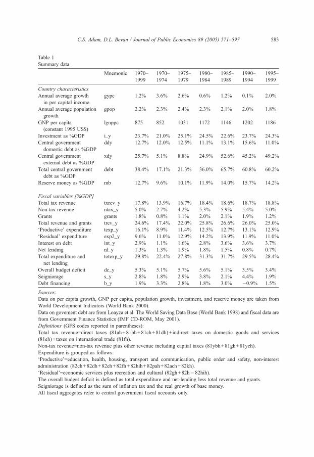
Table 1

Summary data

Mnemonic 1970–

1999

1970–

1974

1975–

1979

1980–

1984

1985–

1989

1990–

1994

1995–

1999

Country characteristics

Annual average growth

in per capital income

gypc 1.2% 3.6% 2.6% 0.6% 1.2% 0.1% 2.0%

Annual average population

growth

gpop 2.2% 2.3% 2.4% 2.3% 2.1% 2.0% 1.8%

GNP per capita

(constant 1995 US$)

lgnppc 875 852 1031 1172 1146 1202 1186

Investment as %GDP i_y 23.7% 21.0% 25.1% 24.5% 22.6% 23.7% 24.3%

Central government

domestic debt as %GDP

ddy 12.7% 12.0% 12.5% 11.1% 13.1% 15.6% 11.0%

Central government

external debt as %GDP

xdy 25.7% 5.1% 8.8% 24.9% 52.6% 45.2% 49.2%

Total central government

debt as %GDP

debt 38.4% 17.1% 21.3% 36.0% 65.7% 60.8% 60.2%

Reserve money as %GDP mb 12.7% 9.6% 10.1% 11.9% 14.0% 15.7% 14.2%

Fiscal variables [%GDP]

Total tax revenue txrev_y 17.8% 13.9% 16.7% 18.4% 18.6% 18.7% 18.8%

Non-tax revenue ntax_y 5.0% 2.7% 4.2% 5.3% 5.9% 5.4% 5.0%

Grants grants 1.8% 0.8% 1.1% 2.0% 2.1% 1.9% 1.2%

Total revenue and grants trev_y 24.6% 17.4% 22.0% 25.8% 26.6% 26.0% 25.0%

dProductiveT expenditure texp_y 16.1% 8.9% 11.4% 12.5% 12.7% 13.1% 12.9%

dResidualT expenditure exp2_y 9.6% 11.0% 12.9% 14.2% 13.9% 11.9% 11.0%

Interest on debt int_y 2.9% 1.1% 1.6% 2.8% 3.6% 3.6% 3.7%

Net lending nl_y 1.3% 1.3% 1.9% 1.8% 1.5% 0.8% 0.7%

Total expenditure and

net lending

totexp_y 29.8% 22.4% 27.8% 31.3% 31.7% 29.5% 28.4%

Overall budget deficit dc_y 5.3% 5.1% 5.7% 5.6% 5.1% 3.5% 3.4%

Seigniorage s_y 2.8% 1.8% 2.9% 3.8% 2.1% 4.4% 1.9%

Debt financing b_y 1.9% 3.3% 2.8% 1.8% 3.0% �0.9% 1.5%

Sources:

Data on per capita growth, GNP per capita, population growth, investment, and reserve money are taken from

World Development Indicators (World Bank 2000).

Data on govement debt are from Loayza et al. The World Saving Data Base (World Bank 1998) and fiscal data are

from Government Finance Statistics (IMF CD-ROM, May 2001).

Definitions (GFS codes reported in parentheses):

Total tax revenue=direct taxes (81ah+81bh+81ch+81dh)+ indirect taxes on domestic goods and services

(81eh)+ taxes on international trade (81fh).

Non-tax revenue=non-tax revenue plus other revenue including capital taxes (81ybh+81gh+81ych).

Expenditure is grouped as follows:

dProductiveT=education, health, housing, transport and communication, public order and safety, non-interest

administration (82ch+82dh+82eh+82fh+82hih+82pah+82ach+82kh).

dResidualT=economic services plus recreation and cultural (82gh+82h�82hih).

The overall budget deficit is defined as total expenditure and net-lending less total revenue and grants.

Seigniorage is defined as the sum of inflation tax and the real growth of base money.

All fiscal aggregates refer to central government fiscal accounts only.



report the coefficients on these time-dummy variables but they are generally strongly

significant and pick up much of the common growth slowdown.25

Estimation of our growth regressions forces us to confront two important econometric

issues. The first concerns the characteristics of the fiscal data. For our sample as a whole,

the principal components of the budget have a much lower variation over time and across

countries than per capita income growth. The cross-country coefficient of variation for per

capita growth is around 2.5 for the pooled data sample but only 0.8 for tax revenue and 0.7

for total non-interest expenditure. The principal exception is the budget deficit itself which

has a sample coefficient of variation of approximately 1.3. The low degree of variability in

fiscal aggregates relative to growth (both across countries and over time) stacks the deck

against finding statistically strong effects from regression analysis of the kind carried out

here, especially for conventional taxation and expenditure aggregates.26

The second problem is that fiscal performance is highly likely to be endogenous to eco-

nomic growth, at least in the short-run.We tackle this in twoways. First, weworkwith (fixed)

5-year averages of the data which eliminates some of the short-run cyclical simultanei-

ty between growth and fiscal performance. Second, we specify our empirical model so that

fiscal factors impact on growth with a lag.27 An obvious alternative strategy is to assume

that fiscal factors and growth are jointly determined and instrument the contemporaneous

effect of fiscal factors on growth. We report the results of estimating our core model in this

manner in Table A2. These suggest that the alternative specification does not change

radically the point estimates, although there is a marked reduction in the precision of the

estimates given the small and unbalanced nature of our panel. In what follows, we there-

fore concentrate our discussion on the results for the case where fiscal effects are lagged.

4. Results and discussion

We start by testing for the presence of thresholds in the impact on growth of the budget

deficit and its financing using the methods developed by Hansen (1999).28 First, let

27 Devarajan et al. (1996) employ a similar strategy. They use annual data and use a 5-year moving average of

the annual growth rate as their dependent variable. Since their sampling interval (annual data) is less than their

moving-average lag, error serial correlation is introduced requiring a correction to the error covariance matrix.

Given the limitations on the fiscal data, we have been unable to estimate our equations at the annual frequency

and hence the issue of overlapping observations does not arise here.

26 Easterly (1995) suggests two reasons why fiscal aggregates, especially revenue shares, have such low

variance. The first is that dnatural experimentsT, in which countries have moved to very high or very low (average)

tax rates, whichwould help identify the impact of revenue and expenditure on growth, are hard to find. This contrasts

to the evidence on inflation and growth where there are numerous extreme inflation episodes allowing the

relationship between inflation and growth to be identified with some precision. The second is that cross-country data

consist only of revenue shares and not marginal rates so that variations in tax rates (which might be substantial) may

not be manifest in tax revenue shares, especially if the informal economy is large and scope for tax evasion exists.

28 This procedure has recently also been applied to examine threshold effects in the relationship between

inflation and growth. See Khan and Senhadji (2001).

25 The median value for the coefficients on the time dummies in the models reported in Table 3, measured

relative to the average growth from 1975 to 1979, are as follows (where the t-values are in parenthesis): 1980–

1984, �1.9% (2.29); 1985–1989, �1.1% (1.26); 1990–1994, �1.7% (1.99); and 1995–1999, �0.9% (1.06).

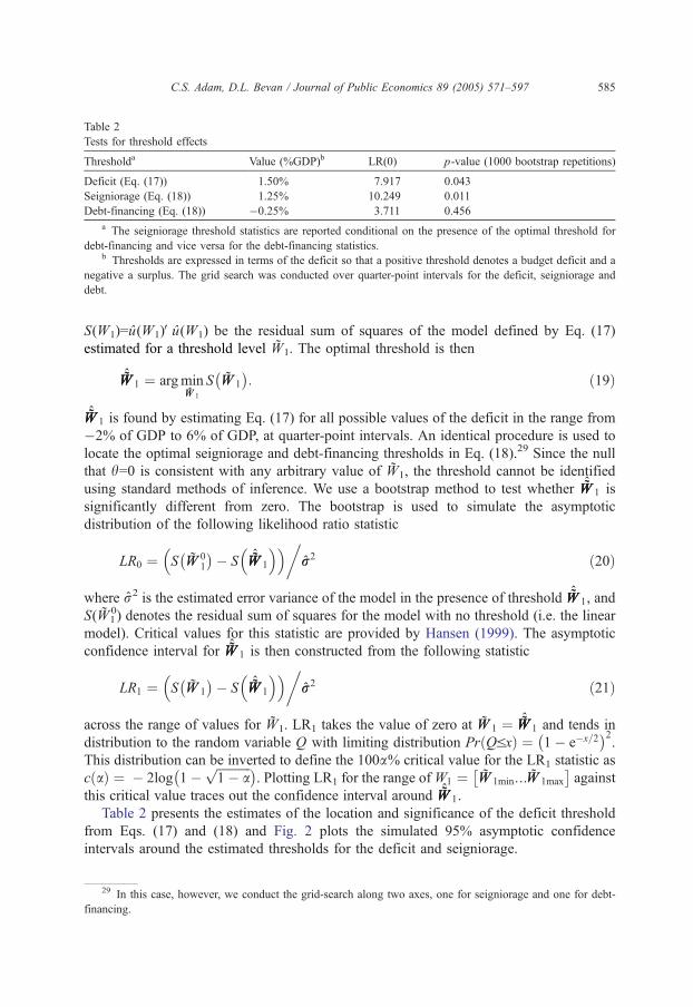
Table 2

Tests for threshold effects

Thresholda Value (%GDP)b LR(0) p-value (1000 bootstrap repetitions)

Deficit (Eq. (17)) 1.50% 7.917 0.043

Seigniorage (Eq. (18)) 1.25% 10.249 0.011

Debt-financing (Eq. (18)) �0.25% 3.711 0.456

a The seigniorage threshold statistics are reported conditional on the presence of the optimal threshold for

debt-financing and vice versa for the debt-financing statistics.b Thresholds are expressed in terms of the deficit so that a positive threshold denotes a budget deficit and a

negative a surplus. The grid search was conducted over quarter-point intervals for the deficit, seigniorage and

debt.


S(W1)=u(W1)Vu(W1) be the residual sum of squares of the model defined by Eq. (17)

estimated for a threshold level W1. The optimal threshold is then

ˆWWWW 1 ¼ argminWW 1

S WW 1

� �: ð19Þ

ˆWWWW 1 is found by estimating Eq. (17) for all possible values of the deficit in the range from

�2% of GDP to 6% of GDP, at quarter-point intervals. An identical procedure is used to

locate the optimal seigniorage and debt-financing thresholds in Eq. (18).29 Since the null

that h=0 is consistent with any arbitrary value of W1, the threshold cannot be identified

using standard methods of inference. We use a bootstrap method to test whether ˆWWWW 1 is

significantly different from zero. The bootstrap is used to simulate the asymptotic

distribution of the following likelihood ratio statistic

LR0 ¼ S WW 01

� �� S ˆWWWW 1

� �� rr2 ð20Þ

where r2 is the estimated error variance of the model in the presence of threshold ˆWWWW 1, and

S(W10) denotes the residual sum of squares for the model with no threshold (i.e. the linear

model). Critical values for this statistic are provided by Hansen (1999). The asymptotic

confidence interval for ˆWWWW 1 is then constructed from the following statistic

LR1 ¼ S WW 1

� �� S ˆWWWW 1

� �� rr2 ð21Þ

across the range of values for W1. LR1 takes the value of zero at WW 1 ¼ ˆWWWW 1 and tends in

distribution to the random variable Q with limiting distribution Pr QVxð Þ ¼ 1� e�x=2� �2

.

This distribution can be inverted to define the 100a% critical value for the LR1 statistic as

c að Þ ¼ � 2log 1�ffiffiffiffiffiffiffiffiffiffiffi1� a

p� �. Plotting LR1 for the range ofW1 ¼ WW 1min N WW 1max

�against

this critical value traces out the confidence interval around ˆWWWW 1.

Table 2 presents the estimates of the location and significance of the deficit threshold

from Eqs. (17) and (18) and Fig. 2 plots the simulated 95% asymptotic confidence

intervals around the estimated thresholds for the deficit and seigniorage.

29 In this case, however, we conduct the grid-search along two axes, one for seigniorage and one for debt-

financing.

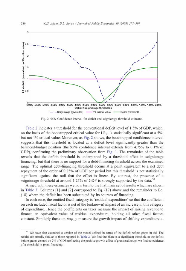
Fig. 2. 95% Confidence interval for deficit and seigniorage threshold estimates.


Table 2 indicates a threshold for the conventional deficit level of 1.5% of GDP, which,

on the basis of the bootstrapped critical value for LR0, is statistically significant at a 5%,

but not 1% critical value. Moreover, as Fig. 2 shows, the bootstrapped confidence interval

suggests that this threshold is located at a deficit level significantly greater than the

balanced-budget position (the 95% confidence interval extends from 4.75% to 0.1% of

GDP), confirming the preliminary observation from Fig. 1. The remainder of the table

reveals that the deficit threshold is underpinned by a threshold effect in seigniorage

financing, but that there is no support for a debt-financing threshold across the examined

range. The optimal debt-financing threshold occurs at a point equivalent to a net debt

repayment of the order of 0.25% of GDP per period but this threshold is not statistically

significant against the null that the effect is linear. By contrast, the presence of a

seigniorage threshold at around 1.25% of GDP is strongly supported by the data.30

Armed with these estimates we now turn to the first main set of results which are shown

in Table 3. Columns [1] and [2] correspond to Eq. (17) above and the remainder to Eq.

(18) where the deficit has been substituted by its sources of financing.

In each case, the omitted fiscal category is dresidual expenditureT so that the coefficient

on each included fiscal factor is net of the (unknown) impact of an increase in this category

of expenditure. Hence the coefficients on taxes measure the impact of raising revenue to

finance an equivalent value of residual expenditure, holding all other fiscal factors

constant. Similarly those on texp_y measure the growth impact of shifting expenditure at

30 We have also examined a version of the model defined in terms of the deficit before grants-in-aid. The

results are broadly similar to those reported in Table 2. We find that there is a significant threshold in the deficit

before grants centred on 2% of GDP (reflecting the positive growth effect of grants) although we find no evidence

of a threshold in grant financing.

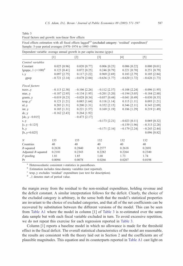
Table 3

Fiscal factors and growth: non-linear flow effects

Fixed effects estimation with all fiscal effects laggeda,b (excluded category: dresidualT expenditure)c

Sample: 5-year period averages (1970–1974 to 1995–1999)

Dependent variable: average annual growth in per capita income (gypc)

[1] [2] [3] [4] [5]

Control variables

Constant 0.025 [0.96] 0.020 [0.77] 0.006 [0.25] 0.006 [0.22] 0.000 [0.01]

lgnppc_1 (100)d 0.123 [0.41] 0.072 [0.25] 0.246 [0.79] 0.221 [0.70] 0.251 [0.79]

i_y 0.097 [2.75] 0.117 [3.22] 0.969 [2.69] 0.103 [2.79] 0.105 [2.84]

gpop �0.721 [2.14] �0.678 [2.04] �0.636 [1.77] �0.620 [1.72] �0.626 [1.73]

Fiscal factors

txrev_y �0.113 [2.38] �0.106 [2.26] �0.112 [2.37] �0.108 [2.24] �0.096 [1.95]

ntax_y �0.187 [2.95] �0.134 [1.95] �0.201 [3.20] �0.194 [3.05] �0.184 [2.88]

grants_y �0.019 [0.23] �0.028 [0.34] �0.037 [0.44] �0.041 [0.49] �0.030 [0.35]

texp_yc 0.121 [1.21] 0.085 [1.64] 0.118 [1.14] 0.115 [1.11] 0.093 [1.21]

nl_y 0.203 [1.31] 0.200 [1.31] 0.352 [2.15] 0.346 [2.11] 0.343 [2.09]

int_y 0.185 [1.31] 0.221 [1.57] 0.169 [1.19] 0.186 [1.29] 0.219 [1.49]

dc_y �0.162 [2.43] 0.264 [1.92]

[dc_y�0.015] �0.473 [2.17]

s_y �0.173 [2.21] �0.023 [0.11] 0.069 [0.32]

[s_y�0.125] �0.159 [1.96] �0.313 [2.28]

b_y �0.171 [2.16] �0.179 [2.24] �0.243 [2.44]

[b_y+0.025] 0.096 [0.82]

N 155 155 132 132 132

Countries 40 40 40 40 40

R-squared 0.2638 0.2840 0.2577 0.2618 0.2691

Adjusted R-squared 0.2181 0.2343 0.2282 0.2264 0.2340

F-pooling 1.81 1.85 1.68 1.73 1.74

Pr 0.0094 0.0078 0.0266 0.0207 0.0198

a Heteroscedastic consistent t-statistics in parentheses.b Estimation includes time-dummy variables (not reported).c texp_y excludes dresidualT expenditure (see text for description).d _1 denotes start of period value.


the margin away from the residual to the non-residual expenditure, holding revenue and

the deficit constant. A similar interpretation follows for the deficit. Clearly, the choice of

the excluded category is arbitrary, in the sense both that the model’s statistical properties

are invariant to the choice of excluded categories, and that all of the net coefficients can be

recovered by substitution between the different versions of the model. This can be seen

from Table A1 where the model in column [1] of Table 3 is re-estimated over the same

data sample but with each fiscal variable excluded in turn. To avoid excessive repetition,

we do not repeat this exercise for each regression reported in Table 3.

Column [1] reports a baseline model in which no allowance is made for the threshold

effect in the fiscal deficit. The overall statistical characteristics of the model are reasonable,

the results are consistent with the theory laid out in Section 2 and the coefficients are of

plausible magnitudes. This equation and its counterparts reported in Table A1 cast light on


the first three of the tax trade-offs discussed in Section 2. Column [1] shows that higher

dresidualT expenditure financed by tax or non-tax revenue significantly reduces average percapita growth in the next period (result (i)) and by a sizeable amount: the coefficient on

txrev_y implies that a tax-financed increase in residual expenditure equivalent to 1% of GDP

would reduce average annual per capita growth in the subsequent period by 0.1 percentage

points. Result (ii) concerned the growth effects of grants. Reading across the grants_y row in

Table A1, we see that grant-financing of lower taxes, higher dproductiveT expenditure, higherother expenditure such as net lending and interest costs, and lower deficits is uniformly

growth-enhancing and for the most part the effects are statistically significant at around the

10% level. By contrast, grant-financing of dresidualT expenditure has no significant impact

on growth. Result (iii) established the conditions under which tax-financing of productive

expenditure will be growth-enhancing. As column [4] of Table A1 shows, however, this

condition is only marginally satisfied and certainly with no statistical significance.

The main focus of this paper, however, is the role of the deficit. Column [1] confirms that,

as expected, the average growth effect of a deficit-financed increase in dresidualT expenditureis negative. In column [2], we introduce the estimated threshold in the deficit from Table 2.

The threshold itself is statistically significant and improves the overall fit of the model, but

does not substantially alter the other coefficients. The implication is that for values of the

deficit less than or equal to the threshold value of 1.5% of GDP a marginal increase in the

deficit is locally growth-enhancing: an increase in the deficit of one percentage point (for

example, from a balanced budget to 1% of GDP) would increase the average annual per

capita growth rate by around one quarter of 1%. By contrast, at levels of the deficit greater

than the threshold the effect is reversed, although the semi-elasticity is of a similar order of

magnitude (0.264�0.473=�0.209). Thus not only does the threshold indicate a change in

the marginal effect but this change is sufficiently large as to suggest a turning point.

The evidence from these first two columns is striking and would appear to point to the

existence of a growth-maximising budget deficit. It is important, though, not to rush too

precipitately to this conclusion, for at least two reasons. The first is that although the

threshold itself is well defined, the interpretation of the coefficient on the fiscal deficit

either side of the threshold remains strictly net of the effect of the excluded fiscal category.

The size (and sign) of the change in the marginal effect of the fiscal deficit around the

threshold will therefore necessarily depend on the expenditure increase or revenue-

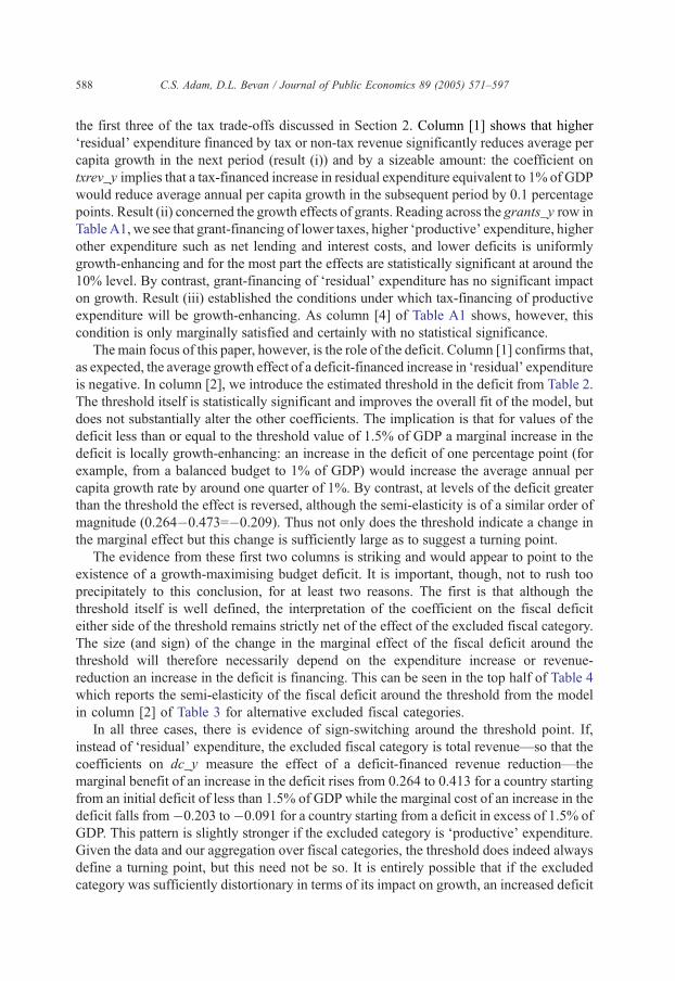
reduction an increase in the deficit is financing. This can be seen in the top half of Table 4

which reports the semi-elasticity of the fiscal deficit around the threshold from the model

in column [2] of Table 3 for alternative excluded fiscal categories.

In all three cases, there is evidence of sign-switching around the threshold point. If,

instead of dresidualT expenditure, the excluded fiscal category is total revenue—so that the

coefficients on dc_y measure the effect of a deficit-financed revenue reduction—the

marginal benefit of an increase in the deficit rises from 0.264 to 0.413 for a country starting

from an initial deficit of less than 1.5% of GDP while the marginal cost of an increase in the

deficit falls from�0.203 to�0.091 for a country starting from a deficit in excess of 1.5% of

GDP. This pattern is slightly stronger if the excluded category is dproductiveT expenditure.Given the data and our aggregation over fiscal categories, the threshold does indeed always

define a turning point, but this need not be so. It is entirely possible that if the excluded

category was sufficiently distortionary in terms of its impact on growth, an increased deficit

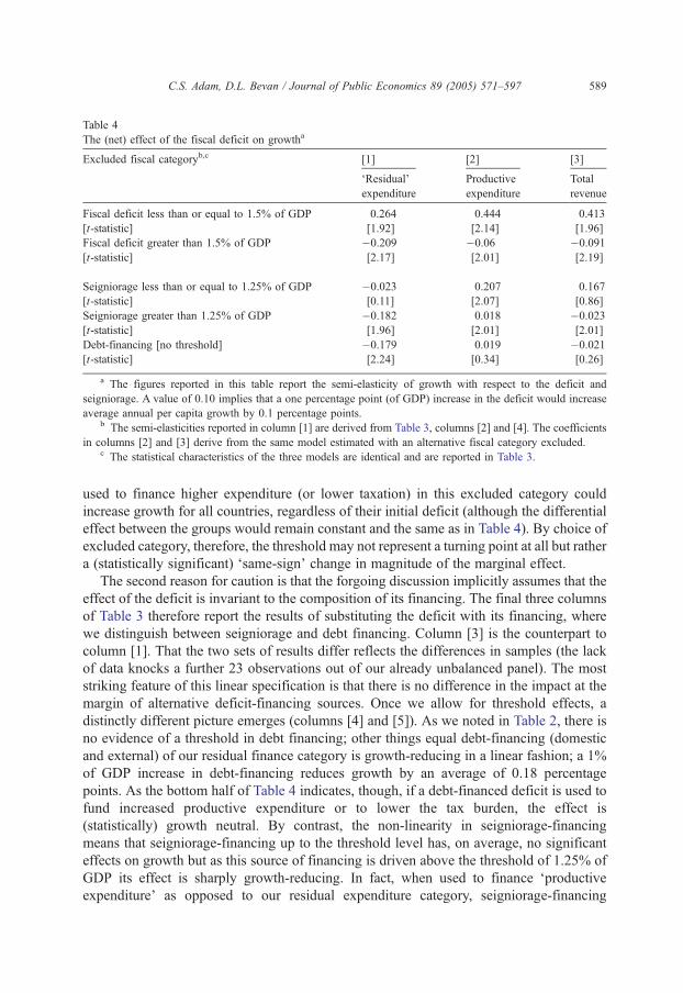
Table 4

The (net) effect of the fiscal deficit on growtha

Excluded fiscal categoryb,c [1] [2] [3]

dResidualTexpenditure

Productive

expenditure

Total

revenue

Fiscal deficit less than or equal to 1.5% of GDP 0.264 0.444 0.413

[t-statistic] [1.92] [2.14] [1.96]

Fiscal deficit greater than 1.5% of GDP �0.209 �0.06 �0.091

[t-statistic] [2.17] [2.01] [2.19]

Seigniorage less than or equal to 1.25% of GDP �0.023 0.207 0.167

[t-statistic] [0.11] [2.07] [0.86]

Seigniorage greater than 1.25% of GDP �0.182 0.018 �0.023

[t-statistic] [1.96] [2.01] [2.01]

Debt-financing [no threshold] �0.179 0.019 �0.021

[t-statistic] [2.24] [0.34] [0.26]

a The figures reported in this table report the semi-elasticity of growth with respect to the deficit and

seigniorage. A value of 0.10 implies that a one percentage point (of GDP) increase in the deficit would increase

average annual per capita growth by 0.1 percentage points.b The semi-elasticities reported in column [1] are derived from Table 3, columns [2] and [4]. The coefficients

in columns [2] and [3] derive from the same model estimated with an alternative fiscal category excluded.c The statistical characteristics of the three models are identical and are reported in Table 3.


used to finance higher expenditure (or lower taxation) in this excluded category could

increase growth for all countries, regardless of their initial deficit (although the differential

effect between the groups would remain constant and the same as in Table 4). By choice of

excluded category, therefore, the threshold may not represent a turning point at all but rather

a (statistically significant) dsame-signT change in magnitude of the marginal effect.

The second reason for caution is that the forgoing discussion implicitly assumes that the

effect of the deficit is invariant to the composition of its financing. The final three columns

of Table 3 therefore report the results of substituting the deficit with its financing, where

we distinguish between seigniorage and debt financing. Column [3] is the counterpart to

column [1]. That the two sets of results differ reflects the differences in samples (the lack

of data knocks a further 23 observations out of our already unbalanced panel). The most

striking feature of this linear specification is that there is no difference in the impact at the

margin of alternative deficit-financing sources. Once we allow for threshold effects, a

distinctly different picture emerges (columns [4] and [5]). As we noted in Table 2, there is

no evidence of a threshold in debt financing; other things equal debt-financing (domestic

and external) of our residual finance category is growth-reducing in a linear fashion; a 1%

of GDP increase in debt-financing reduces growth by an average of 0.18 percentage

points. As the bottom half of Table 4 indicates, though, if a debt-financed deficit is used to

fund increased productive expenditure or to lower the tax burden, the effect is

(statistically) growth neutral. By contrast, the non-linearity in seigniorage-financing

means that seigniorage-financing up to the threshold level has, on average, no significant

effects on growth but as this source of financing is driven above the threshold of 1.25% of

GDP its effect is sharply growth-reducing. In fact, when used to finance dproductiveexpenditureT as opposed to our residual expenditure category, seigniorage-financing

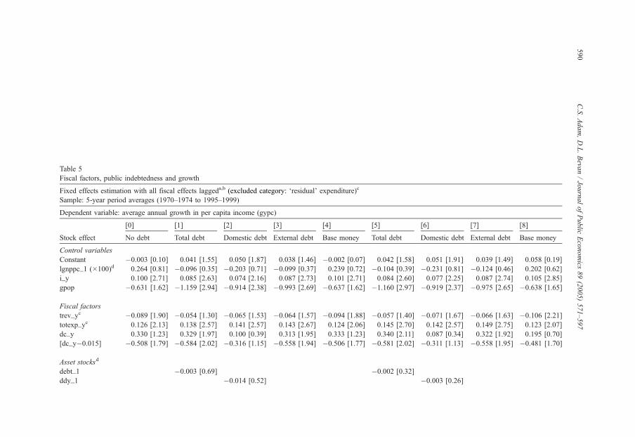
Table 5

Fiscal factors, public indebtedness and growth

Fixed effects estimation with all fiscal effects laggeda,b (excluded category: dresidualT expenditure)c



[0] [1] [2] [3] [4] [5] [6] [7] [8]

Stock effect No debt Total debt Domestic debt External debt Base money Total debt Domestic debt External debt Base money

Control variables

Constant �0.003 [0.10] 0.041 [1.55] 0.050 [1.87] 0.038 [1.46] �0.002 [0.07] 0.042 [1.58] 0.051 [1.91] 0.039 [1.49] 0.058 [0.19]

lgnppc_1 (100)d 0.264 [0.81] �0.096 [0.35] �0.203 [0.71] �0.099 [0.37] 0.239 [0.72] �0.104 [0.39] �0.231 [0.81] �0.124 [0.46] 0.202 [0.62]

i_y 0.100 [2.71] 0.085 [2.63] 0.074 [2.16] 0.087 [2.73] 0.101 [2.71] 0.084 [2.60] 0.077 [2.25] 0.087 [2.74] 0.105 [2.85]

gpop �0.631 [1.62] �1.159 [2.94] �0.914 [2.38] �0.993 [2.69] �0.637 [1.62] �1.160 [2.97] �0.919 [2.37] �0.975 [2.65] �0.638 [1.65]

Fiscal factors

trev_yc �0.089 [1.90] �0.054 [1.30] �0.065 [1.53] �0.064 [1.57] �0.094 [1.88] �0.057 [1.40] �0.071 [1.67] �0.066 [1.63] �0.106 [2.21]

totexp_yc 0.126 [2.13] 0.138 [2.57] 0.141 [2.57] 0.143 [2.67] 0.124 [2.06] 0.145 [2.70] 0.142 [2.57] 0.149 [2.75] 0.123 [2.07]

dc_y 0.330 [1.23] 0.329 [1.97] 0.100 [0.39] 0.313 [1.95] 0.333 [1.23] 0.340 [2.11] 0.087 [0.34] 0.322 [1.92] 0.195 [0.70]

[dc_y�0.015] �0.508 [1.79] �0.584 [2.02] �0.316 [1.15] �0.558 [1.94] �0.506 [1.77] �0.581 [2.02] �0.311 [1.13] �0.558 [1.95] �0.481 [1.70]

Asset stocksd

debt_1 �0.003 [0.69] �0.002 [0.32]

ddy_1 �0.014 [0.52] �0.003 [0.26]

C.S.Adam,D.L.Beva

n/JournalofPublic

Economics

89(2005)571–597

590

xdy_1 �0.004 [1.17] �0.002 [0.29]

mb_1 0.019 [0.37] 0.004 [0.83]

Stock interactionse

D*debt_1 �0.055 [1.84]

D*ddy_1 0.030 [0.10]

D*xdy_1 �0.068 [1.96]

D*mb_1 0.777 [1.86]

N 123 119 122 123 121 119 122 123 123

Countries 31 31 31 31 30 31 31 31 31

R-squared 0.2697 0.2694 0.2572 0.259 0.271 0.2744 0.2566 0.2621 0.2889

Adjusted R-squared 0.2252 0.2233 0.2116 0.2139 0.2258 0.2286 0.2110 0.2172 0.2456

F-pooling 1.51 1.65 1.83 1.64 2.04 1.40 1.8 1.43 2.04

Pr 0.00732 0.0104 0.0025 0.0113 0.0015 0.1203 0.0202 0.1058 0.0067

Column [0] reports basic model from Table 3 estimated over reduced sample.a Heteroscedastic consistent t-statistics in parentheses.b Estimation includes time-dummy variables (not reported).c trev_y= txrev_y+ntax_y+grants_y; totexp_y= texp_y+nl_y+ int_y (see text for description).d _1 denotes start of period value.e Interactions variables D*X denote the interaction of dc_y with variable X.

C.S.Adam,D.L.Beva

n/JournalofPublic

Economics

89(2005)571–597

591


appears to be significantly growth-enhancing below the threshold and has no negative

effect on growth above the threshold (at least locally). A similar effect results if we let the

excluded fiscal category be total revenue.

Given our inability to consistently disaggregate debt-financing, we have been unable to

directly test results (iv) to (vi) from Section 2. However, our empirical results do offer

broad support to the model, in particular by showing that while the effect of debt-financing

appears to be linear (and significantly negative when financing dresidualT expenditure)

there is a significant non-linearity in seigniorage-financing consistent with growth-

enhancing moderate deficit-financing, particularly when seigniorage is used to finance

productive expenditure or to write down taxes.

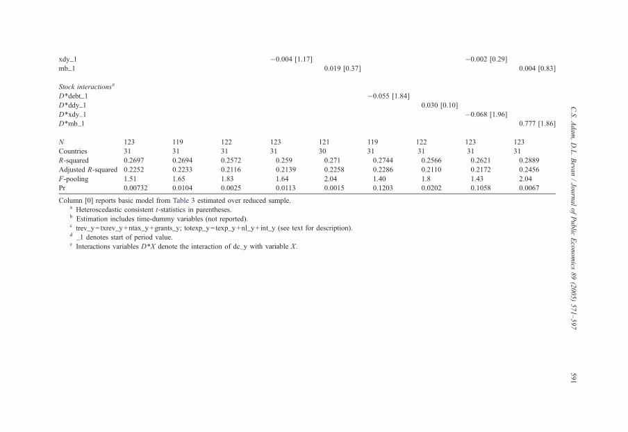
The final step in the analysis interacts the deficit with the level of public indebtedness

(Table 5).31 We disaggregate total government indebtedness into its interest-bearing

components, namely domestic and external debt, and base money, each expressed as a

share of GDP.32 To focus on these stock effects, we simplify the model slightly by

including only total revenue and total expenditure (excluding dresidualT expenditure whichremains the excluded fiscal category). This aggregation makes no substantial difference to

the results on the effect of the deficit.

Despite the poor quality of the data and the reduction in the usable sample size, a

number of interesting features emerge from Table 5. Either on its own or interacted with

the flow deficit, the degree of public indebtedness does not greatly alter the overall

characteristics of the model or the values of the coefficients on total revenue and total

expenditure, despite the reduction in the usable sample size. Column [0], which reports the

counterpart to the basic model from Table 3 but estimated over the reduced sample,

suggests that the broad characteristics of the basic model are robust to this particular

change in the sample. Importantly, controlling for debt stocks does not eliminate the non-

linearity on the flow effect of the deficit.33,34

This aside, the level of public indebtedness matters for growth in a consistent manner,

even though the measured effects are not strongly significant, particularly for domestic debt.

Higher levels of interest-bearing debt (columns [1] to [3]) are associated with lower future

growth, while higher real money demand is associated with higher future growth (column

[4]). However, it is through their interaction with the flow deficit that the external indebted-

ness and the stock of high-powered money appear to have their main effect (columns [5] to

[8]). To help interpret these results, Table 6 reports the effects of the fiscal deficit on growth

evaluated at alternative levels of external indebtedness and real money demand.

31 Ideally, we would be able to examine the consequences of the level of indebtedness on the impact of the

deficit and its financing. Attempting to interact indebtedness with deficit financing we confront a dramatic

reduction in usable observations; the panel shrinks from around 155 observations to less than 80. Since this

severely undermines our ability to compare results, we limit ourselves in this section to examining only the

relationship between the flow deficit and measures of total indebtedness.32 The measure of external indebtedness, taken from Loayza et al. (1998), does not adjust for the degree of

concessionality of external debt.33 Controlling for the stock of indebtedness, we obtain the same estimates of the location and significance of

the optimal thresholds for the deficit and seigniorage as reported in Table 2.34 It is also interesting to note that the inclusion of public indebtedness, principally external indebtedness,

eliminates the country-specific effects. Conditional on the other variables in the model external indebtedness thus

provides a summary statistic for otherwise unobservable country heterogeneity in growth patterns.

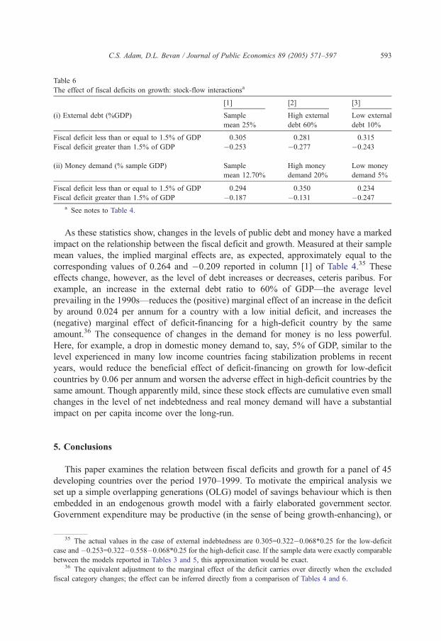
Table 6

The effect of fiscal deficits on growth: stock-flow interactionsa

[1] [2] [3]

(i) External debt (%GDP) Sample

mean 25%

High external

debt 60%

Low external

debt 10%



(ii) Money demand (% sample GDP) Sample

mean 12.70%

High money

demand 20%

Low money

demand 5%



a See notes to Table 4.


As these statistics show, changes in the levels of public debt and money have a marked

impact on the relationship between the fiscal deficit and growth. Measured at their sample

mean values, the implied marginal effects are, as expected, approximately equal to the

corresponding values of 0.264 and �0.209 reported in column [1] of Table 4.35 These

effects change, however, as the level of debt increases or decreases, ceteris paribus. For

example, an increase in the external debt ratio to 60% of GDP—the average level

prevailing in the 1990s—reduces the (positive) marginal effect of an increase in the deficit

by around 0.024 per annum for a country with a low initial deficit, and increases the

(negative) marginal effect of deficit-financing for a high-deficit country by the same

amount.36 The consequence of changes in the demand for money is no less powerful.

Here, for example, a drop in domestic money demand to, say, 5% of GDP, similar to the

level experienced in many low income countries facing stabilization problems in recent

years, would reduce the beneficial effect of deficit-financing on growth for low-deficit

countries by 0.06 per annum and worsen the adverse effect in high-deficit countries by the

same amount. Though apparently mild, since these stock effects are cumulative even small

changes in the level of net indebtedness and real money demand will have a substantial

impact on per capita income over the long-run.

5. Conclusions

This paper examines the relation between fiscal deficits and growth for a panel of 45

developing countries over the period 1970–1999. To motivate the empirical analysis we

set up a simple overlapping generations (OLG) model of savings behaviour which is then

embedded in an endogenous growth model with a fairly elaborated government sector.

Government expenditure may be productive (in the sense of being growth-enhancing), or

35 The actual values in the case of external indebtedness are 0.305=0.322�0.068*0.25 for the low-deficit

case and �0.253=0.322�0.558�0.068*0.25 for the high-deficit case. If the sample data were exactly comparable

between the models reported in Tables 3 and 5, this approximation would be exact.36 The equivalent adjustment to the marginal effect of the deficit carries over directly when the excluded

fiscal category changes; the effect can be inferred directly from a comparison of Tables 4 and 6.


unproductive, and there is an output tax which is growth-inhibiting. However, the

government budget need not be balanced. There are thus two types of government

spending, and five ways of financing it, taxes, grants and three forms of deficit finance (by

printing money, and by issuing domestic or external debt). The analysis suggests that

while the impacts on growth of taxes and grants are reasonably straightforward, the impact

of the deficit is likely to be complex, depending on the financing mix and the outstanding

debt stock. In particular, deficits may be growth-enhancing if financed by limited

seigniorage; they are likely to be growth-inhibiting if financed by domestic debt; and to

have opposite flow and stock effects if financed by external loans at market rates. In

particular, two types of non-linearity may emerge, one involving the size of the deficit and

the other interactions between the deficit and the public debt stock.

At a casual level, the scatterplot for our 45 countries in Fig. 1 does suggest a possible

non-linearity in the relation between growth and the fiscal deficit for this sample. More

formally, our econometric analysis, based on a consistent treatment of the government

budget constraint, confirms the existence of these stock–flow interactions and identifies a

threshold effect in the deficit which is robust to their inclusion. This threshold effect is at a

level of the deficit (after grants) around 1.5% of GDP. While there appears to be a growth

payoff to reducing deficits to this level, this effect disappears or reverses itself for further

fiscal contraction. The magnitude of this payoff, but not its general character, necessarily

depends on how changes in the deficit are financed (through changes in borrowing or

seigniorage) and on how the change in the deficit is accommodated elsewhere in the

budget. The thresholds involve not only a change of slope but also a change of sign in the

relation regardless of the budget category excluded from the model, indicating that for an

economy not on its steady state growth path, there is a range over which deficit-financing

may be growth-enhancing. We also find evidence of interaction effects between deficits and

debt stocks, with high debt stocks exacerbating the adverse consequences of high deficits.

Acknowledgement

The original version of this paper was prepared for the Cornell/ISPE Conference on

Public Finance and Development held at Cornell University, September 7–9, 2001. We

thank our discussant, Mick Keen, conference and seminar participants at Cornell, Oxford

and Clermont-Ferrand, and also Jon Temple for helpful comments on the original version,

and two referees for very insightful comments on the revised version.

Appendix A. Sample countries

Argentina, Bahrain, Barbados, Bhutan, Brazil, Bulgaria, Cameroon, Chile, Colombia,

Costa Rica, Dominican Republic, Egypt, El Salvador, Ghana, Honduras, Hungary, India,

Indonesia, Israel, Kenya, Korea, Lebanon, Lesotho, Malaysia, Mali, Mauritius, Mexico,

Morocco, Nicaragua, Peru, Panama, Paraguay, Poland, Romania, Senegal, Singapore,

South Africa, Sri Lanka, Suriname, Thailand, Togo, Tunisia, Uruguay, Zambia, Zimbabwe.

Tables A1 and A2.

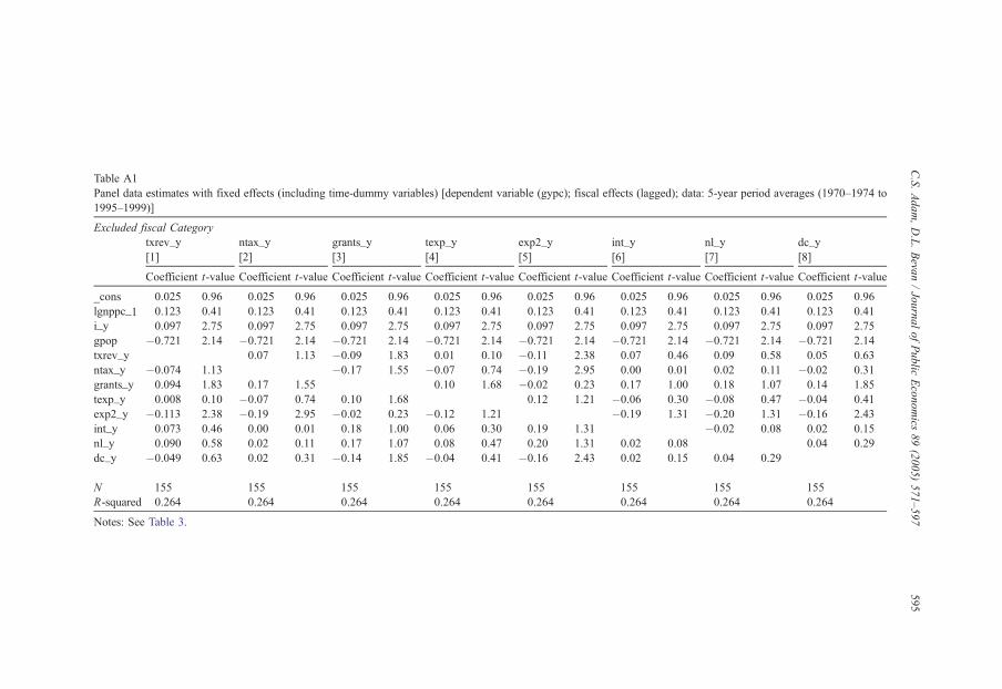
Table A1

Panel data estimates with fixed effects (including time-dummy variables) [dependent variable (gypc); fiscal effects (lagged); data: 5-year period averages (1970–1974 to

1995–1999)]

Excluded fiscal Category

txrev_y ntax_y grants_y texp_y exp2_y int_y nl_y dc_y

[1] [2] [3] [4] [5] [6] [7] [8]

Coefficient t-value Coefficient t-value Coefficient t-value Coefficient t-value Coefficient t-value Coefficient t-value Coefficient t-value Coefficient t-value

_cons 0.025 0.96 0.025 0.96 0.025 0.96 0.025 0.96 0.025 0.96 0.025 0.96 0.025 0.96 0.025 0.96

lgnppc_1 0.123 0.41 0.123 0.41 0.123 0.41 0.123 0.41 0.123 0.41 0.123 0.41 0.123 0.41 0.123 0.41

i_y 0.097 2.75 0.097 2.75 0.097 2.75 0.097 2.75 0.097 2.75 0.097 2.75 0.097 2.75 0.097 2.75

gpop �0.721 2.14 �0.721 2.14 �0.721 2.14 �0.721 2.14 �0.721 2.14 �0.721 2.14 �0.721 2.14 �0.721 2.14

txrev_y 0.07 1.13 �0.09 1.83 0.01 0.10 �0.11 2.38 0.07 0.46 0.09 0.58 0.05 0.63

ntax_y �0.074 1.13 �0.17 1.55 �0.07 0.74 �0.19 2.95 0.00 0.01 0.02 0.11 �0.02 0.31

grants_y 0.094 1.83 0.17 1.55 0.10 1.68 �0.02 0.23 0.17 1.00 0.18 1.07 0.14 1.85

texp_y 0.008 0.10 �0.07 0.74 0.10 1.68 0.12 1.21 �0.06 0.30 �0.08 0.47 �0.04 0.41

exp2_y �0.113 2.38 �0.19 2.95 �0.02 0.23 �0.12 1.21 �0.19 1.31 �0.20 1.31 �0.16 2.43

int_y 0.073 0.46 0.00 0.01 0.18 1.00 0.06 0.30 0.19 1.31 �0.02 0.08 0.02 0.15

nl_y 0.090 0.58 0.02 0.11 0.17 1.07 0.08 0.47 0.20 1.31 0.02 0.08 0.04 0.29

dc_y �0.049 0.63 0.02 0.31 �0.14 1.85 �0.04 0.41 �0.16 2.43 0.02 0.15 0.04 0.29

N 155 155 155 155 155 155 155 155

R-squared 0.264 0.264 0.264 0.264 0.264 0.264 0.264 0.264

Notes: See Table 3.

C.S.Adam,D.L.Beva

n/JournalofPublic

Economics

89(2005)571–597

595

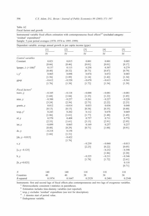
Table A2

Fiscal factors and growth

Instrumental variable fixed effects estimation with contemporaneous fiscal effectsa,b (excluded category:

dresidualT expenditure)c



[1] [2] [3] [4] [5]

IV IV IV IV IV

Control variables

Constant 0.021 0.015 0.001 0.001 0.005

[0.66] [0.46] [0.01] [0.01] [0.17]

lgnppc_1 (100)d 0.137 0.113 0.258 0.307 0.279

[0.40] [0.32] [0.73] [0.87] [0.79]

i_ye 0.065 0.098 0.074 0.072 0.085

[1.56] [1.89] [1.14] [1.42] [1.34]

gpop �0.612 �0.520 �0.670 �0.613 �0.561

[1.76] [1.38] [1.72] [1.54] [1.39]

Fiscal factorse

txrev_y �0.105 �0.118 �0.088 �0.081 �0.081

[1.68] [1.84] [1.35] [1.22] [1.85]

ntax_y �0.300 �0.257 �0.261 �0.227 �0.228

[3.24] [2.56] [2.73] [2.22] [2.23]

grants_y 0.012 �0.014 0.033 0.036 0.040

[0.13] [0.13] [0.34] [0.35] [0.40]

texp_yc 0.243 0.202 0.112 0.078 0.069

[1.86] [1.61] [1.77] [1.48] [1.45]

nl_y 0.570 0.408 0.757 0.711 0.778

[2.33] [1.61] [3.13] [2.91] [2.95]

int_y �0.099 0.065 0.169 0.257 0.237

[0.48] [0.29] [0.71] [1.00] [0.91]

dc_y �0.218 0.158

[1.66] [1.31]

[dc_y�0.015] �0.422

[1.76]

s_y �0.239 �0.060 �0.013

[2.23] [0.22] [0.05]

[s_y�0.125] �0.232 �0.398

[1.86] [2.20]

b_y �0.225 �0.211 �0.346

[1.78] [1.72] [2.61]

[b_y+0.025] 0.118

[0.71]

N 140 140 118 118 118

Countries 40 40 38 38 38

R-squared 0.1974 0.1647 0.2529 0.2481 0.2548

Instruments: first and second lags of fiscal effects plus contemporaneous and two lags of exogenous variables.a Heteroscedastic consistent t-statistics in parentheses.b Estimation includes time-dummy variables (not reported).c texp_y excludes dresidualT expenditure (see text for description).d _1 denotes start of period value.e Endogenous variable.



Appendix B. Supplementary data

Supplementary data associated with this article can be found, in the online version, at

doi:10.1016/j.jpubeco.2004.02.006.

References

Aghion, P., Howitt, P., 1998. Endogenous Growth Theory. MIT Press, Cambridge, MA.

Barro, R., 1990. Government spending in a simple model of endogenous growth. Journal of Political Economy

98, S103–S125.

Barro, R., Sala-I-Martin, X., 1992. Public finance in models of economic growth. Review of Economic Studies

59, 645–661.

Barro, R., Sala-I-Martin, X., 1995. Economic Growth. McGraw-Hill, New York.

Devarajan, S., Swaroop, V., Zou, H.-F., 1996. The composition of public expenditure and economic growth.

Journal of Monetary Economics 37, 313–344.

Diamond, P., 1965. National debt in a neoclassical growth model. American Economic Review 55, 1126–1150.

Easterly, W., 1995. Comments on: Joel Slemrod bWhat do cross-country studies teach about government

involvement, prosperity, and economic growth?Q Brookings Papers on Economic Activity 2, 373–431.

Easterly, W., Rodriguez, C., Schmidt-Hebbel, K. (Eds.), 1994. Public sector deficits and macroeconomic

performance, Oxford and New York, OUP and the World Bank.

Gemmell, N., 2001. Fiscal policy in a growth framework. WIDER Discussion Paper 2001/84.

Giavazzi, F., Japelli, T., Pagano, M., 2000. Searching for non-linear effects of fiscal policy: evidence from

industrial and developing countries. European Economic Review 44, 1259–1289.

Hansen, B., 1999. Threshold effects in non-dynamic panels: estimation, testing and inference. Journal of

Econometrics 93, 345–368.

Khan, M., Senhadji, A., 2001. Threshold effects in the relationship between inflation and growth. IMF Staff

Papers 48, 1–21.

Kneller, R., Bleaney, M., Gemmell, N., 2000. Fiscal policy and growth: evidence from OECD countries. Journal

of Public Economics 74, 171–190.

Loayza, N., Lopez, H., Schmidt-Hebbel, K., Serven, L., 1998. The World Saving Data Base. World Bank, mimeo.

Miller, S., Russek, F., 1997. Fiscal structures and economic growth: international evidence. Economic Enquiry

35, 603–613.

Robinson, P., 1988. Root-N consistent semiparametric regression. Econometrica 56, 931–954.

Yatchew, A., 1998. An elementary estimator of the partial linear model. Economics Letters 57, 135–143.

http://dx.doi.org/doi:10.1016/j.jpubeco.2004.02.006

fiscal deficits and growth in developing countries · this paper examines the relation between...

Documents