fiscal multipliers in practice - regjeringen.no · 4 the use of fiscal multipliers at the fund is...
TRANSCRIPT

Fiscal Multipliers in Practice
Marcos Poplawski-Ribeiro
Meeting of the Advisory Panel on Macro-economic Models and Methods – Norway Ministry of Finance
Oslo, June 3, 2013
2
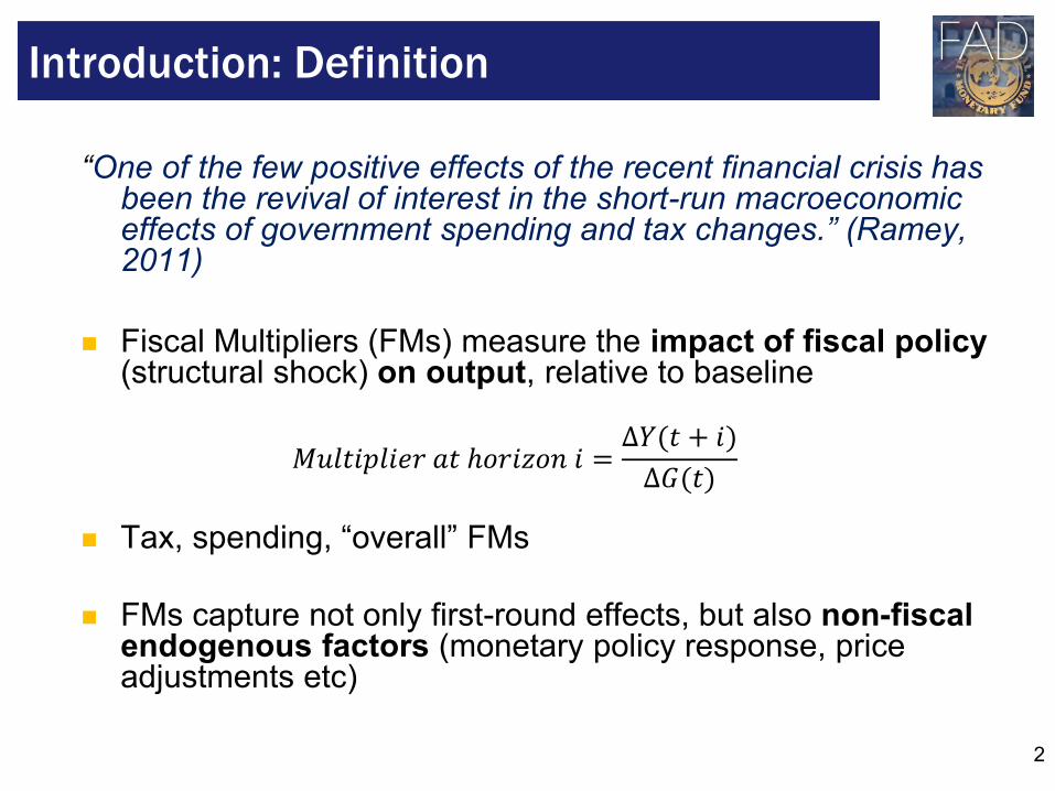
“One of the few positive effects of the recent financial crisis has been the revival of interest in the short-run macroeconomic effects of government spending and tax changes.” (Ramey, 2011)
Fiscal Multipliers (FMs) measure the impact of fiscal policy
(structural shock) on output, relative to baseline
Tax, spending, “overall” FMs
FMs capture not only first-round effects, but also non-fiscal endogenous factors (monetary policy response, price adjustments etc)
Introduction: Definition
𝑀𝑢𝑙𝑡𝑖𝑝𝑙𝑖𝑒𝑟 𝑎𝑡 ℎ𝑜𝑟𝑖𝑧𝑜𝑛 𝑖 =∆𝑌(𝑡 + 𝑖)
∆𝐺(𝑡)
3
I. Introduction
II. Methodology
III. Literature
I. Mineshima et al.(2013)
II. Survey on Non-linear Fiscal Multipliers
III. Literature Survey on Asia
IV. Estimation
I. Baum, Poplawski-Ribeiro, and Weber (2012)
V. Use
VI. Conclusions
VII. Appendices
Overview

4
The use of fiscal multipliers at the Fund is heterogeneous
Average 1-year multiplier = 0.5
Heterogeneity is to be expected
FMs estimates not available for most EMs and LICs
In financial programming, not all countries (in particular LICs) model feedback from fiscal to real sector
Country teams implicitly take into account fiscal policy in their growth projections
Introduction: Motivation (1)
Introduction Literature Estimation Use Method
5
More systematic use of FMs could be beneficial:
May improve the accuracy of growth
projections (Blanchard and Leigh, 2013;
Beetsma et al. 2010)
May improve policy advice and program design.
Underestimating FMs creates risks: unachievable
targets; negative feedback loops of repeated
tightening-slow growth-deflation
Introduction: Motivation (2)
Introduction Literature Estimation Use Method
6
Step 1: How is the right Fiscal Multiplier selected?
Three main options:
Estimate via (S)VAR or DSGE
Use existing estimates if (i) available, (ii) meet certain quality
standards, (iii) take into account amplifying factors of current
environment
Guesstimate with “bucket” approach (in particular for EMs
and LICs). Can also serve as cross-check
General Approach (1)
Introduction Literature Estimation Use Method
7
Step 2: How are Fiscal Multipliers incorporated
into macro projections?
Not straightforward how to integrate Fiscal Multipliers in
the financial programming framework
However, there are alternative methods to account for
fiscal policy in growth forecasts
Additional option: incorporate FMs via a template
General Approach (2)
Introduction Literature Estimation Use Method
8
Two types of estimates in the literature: (i) empirical; (ii) model-based
Recent empirical literature on advanced economies
(S)VAR using country-specific data
Important to specify clearly the identification strategy
Reflect average output response over the past
Time-varying multipliers? (Cimadomo & Bénassy-Quéré, 2012)
May fail to measure correctly exogenous fiscal shocks
Also how to account for other shocks (monetary) and spillovers
Model: DSGE estimates (e.g., GIMF, or EC or OECD models)
Describe whole economy, more variables (Coenen et al., 2012)
Results partly pre-determined; less cross-country dispersion of FMs
How to get Multipliers “Off-The-Shelf”? (1)
Introduction Literature Estimation Use Method
9
Advanced economies
Mineshima, Poplawski-Ribeiro, and Weber (2013) broad review of past literature (empirical and model): Average 1-year Fiscal Multipliers <1
0.5-0.9 for G; 0.1-0.3 for T
→ based on current exp-rev mix, this gives an overall FM of 0.6
More recently: Fiscal Multipliers may be larger in current environment:
i. downturn;
ii. less supportive external environment; and
iii. policy interest rate close to the zero lower bound
How to get Multipliers “Off-The-Shelf”? (2)
Introduction Literature Estimation Use Method
10
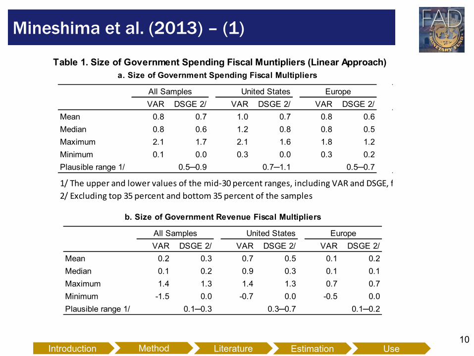
Mineshima et al. (2013) – (1)
Introduction Literature Estimation Use Method
VAR DSGE 2/ VAR DSGE 2/ VAR DSGE 2/
Mean 0.8 0.7 1.0 0.7 0.8 0.6
Median 0.8 0.6 1.2 0.8 0.8 0.5
Maximum 2.1 1.7 2.1 1.6 1.8 1.2
Minimum 0.1 0.0 0.3 0.0 0.3 0.2
Plausible range 1/
1/ The upper and lower values of the mid-30 percent ranges, including VAR and DSGE, from Box 1.
2/ Excluding top 35 percent and bottom 35 percent of the samples
a. Size of Government Spending Fiscal Multipliers
All Samples United States Europe
Table 1. Size of Government Spending Fiscal Muntipliers (Linear Approach)
0.5─0.9 0.7─1.1 0.5─0.7
VAR DSGE 2/ VAR DSGE 2/ VAR DSGE 2/
Mean 0.2 0.3 0.7 0.5 0.1 0.2
Median 0.1 0.2 0.9 0.3 0.1 0.1
Maximum 1.4 1.3 1.4 1.3 0.7 0.7
Minimum -1.5 0.0 -0.7 0.0 -0.5 0.0
Plausible range 1/
b. Size of Government Revenue Fiscal Multipliers
All Samples United States Europe
0.1─0.20.1─0.3 0.3─0.7
11
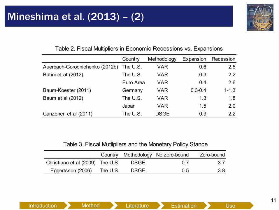
Mineshima et al. (2013) – (2)
Introduction Literature Estimation Use Method
Country Methodology Expansion Recession
Auerbach-Gorodnichenko (2012b) The U.S. VAR 0.6 2.5
Batini et at (2012) The U.S. VAR 0.3 2.2
Euro Area VAR 0.4 2.6
Baum-Koester (2011) Germany VAR 0.3-0.4 1-1.3
Baum et al (2012) The U.S. VAR 1.3 1.8
Japan VAR 1.5 2.0
Canzonen et al (2011) The U.S. DSGE 0.9 2.2
Table 2. Fiscal Multipliers in Economic Recessions vs. Expansions
Country Methodology No zero-bound Zero-bound
Christiano et al (2009) The U.S. DSGE 0.7 3.7
Eggertsson (2006) The U.S. DSGE 0.5 3.8
Table 3. Fiscal Mutlipliers and the Monetary Policy Stance
12
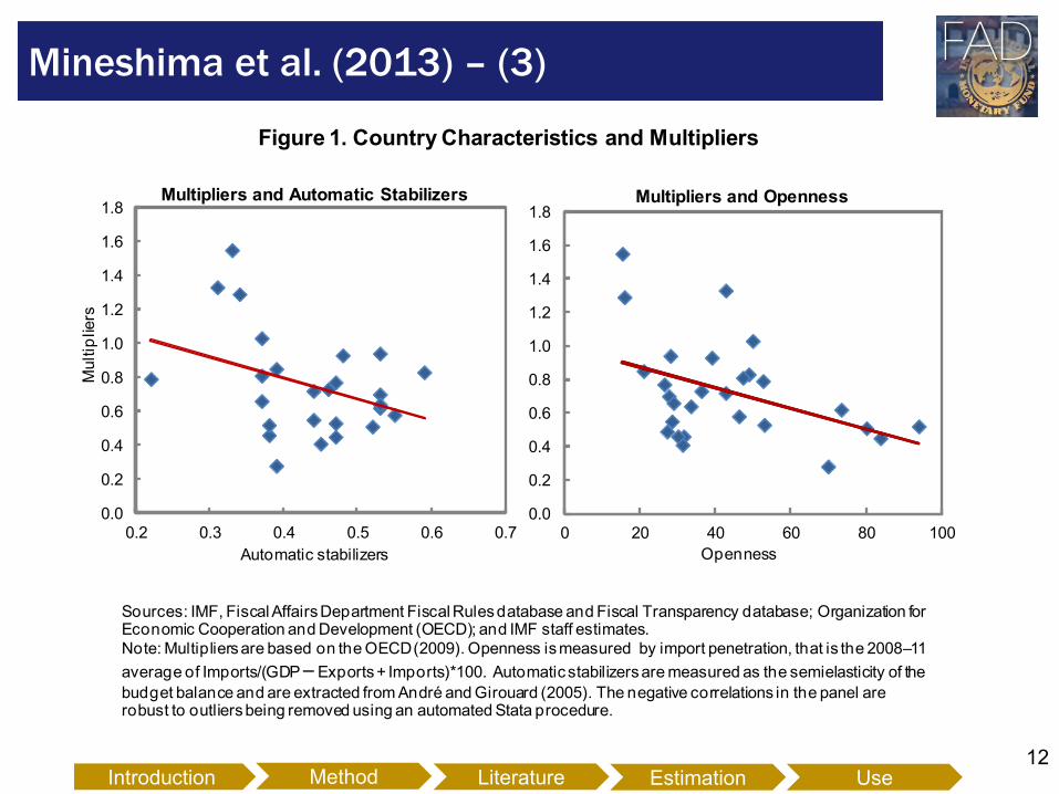
Mineshima et al. (2013) – (3)
Introduction Literature Estimation Use Method
Figure 1. Country Characteristics and Multipliers
Sources: IMF, Fiscal Affairs Department Fiscal Rules database and Fiscal Transparency database; Organization for Economic Cooperation and Development (OECD); and IMF staff estimates.
Note: Multipliers are based on the OECD (2009). Openness is measured by import penetration, that is the 2008–11
average of Imports/(GDP– Exports + Imports)*100. Automatic stabilizers are measured as the semielasticity of the
budget balance and are extracted from André and Girouard (2005). The negative correlations in the panel are robust to outliers being removed using an automated Stata procedure.
0.0
0.2
0.4
0.6
0.8
1.0
1.2
1.4
1.6
1.8
0 20 40 60 80 100
Openness
Multipliers and Openness
0.0
0.2
0.4
0.6
0.8
1.0
1.2
1.4
1.6
1.8
0.2 0.3 0.4 0.5 0.6 0.7
Automatic stabilizers
Multipliers and Automatic Stabilizers
Multip
liers
13
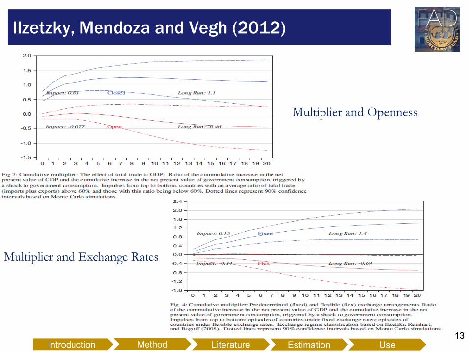
Ilzetzky, Mendoza and Vegh (2012)
Introduction Literature Estimation Use Method
Multiplier and Openness
Multiplier and Exchange Rates
14
Emerging economies and LICs
Limited evidence (Ilzetzki 2011, Ilzetzki et al. 2011)
FMs seem to be smaller than in advanced economies
Maybe due to more open economies, higher spreads,
supply and capacity constraints, precautionary savings?
Fiscal policy implementation in LICs: Lledó & Poplawski-Ribeiro
(2012) and Guerguil and others (2013).
How to get Multipliers “Off-The-Shelf”? (3)
Introduction Literature Estimation Use Method
15
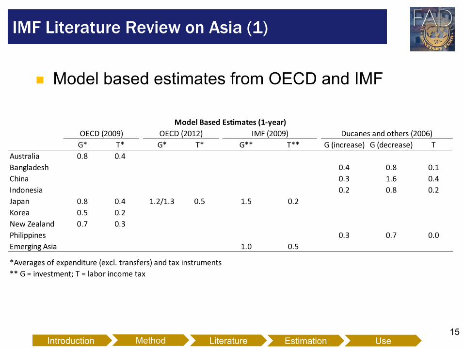
Model based estimates from OECD and IMF
IMF Literature Review on Asia (1)
Introduction Literature Estimation Use Method
G* T* G* T* G** T** G (increase) G (decrease) T
Australia 0.8 0.4
Bangladesh 0.4 0.8 0.1
China 0.3 1.6 0.4
Indonesia 0.2 0.8 0.2
Japan 0.8 0.4 1.2/1.3 0.5 1.5 0.2
Korea 0.5 0.2
New Zealand 0.7 0.3
Philippines 0.3 0.7 0.0
Emerging Asia 1.0 0.5
*Averages of expenditure (excl. transfers) and tax instruments
** G = investment; T = labor income tax
OECD (2009) OECD (2012) Ducanes and others (2006)
Model Based Estimates (1-year)
IMF (2009)
16
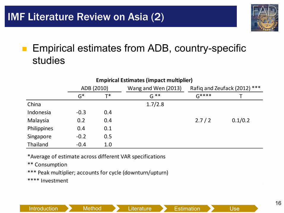
Empirical estimates from ADB, country-specific
studies
IMF Literature Review on Asia (2)
Introduction Literature Estimation Use Method
Wang and Wen (2013)
G* T* G ** G**** T
China 1.7/2.8
Indonesia -0.3 0.4
Malaysia 0.2 0.4 2.7 / 2 0.1/0.2
Philippines 0.4 0.1
Singapore -0.2 0.5
Thailand -0.4 1.0
*Average of estimate across different VAR specifications
** Consumption
*** Peak multiplier; accounts for cycle (downturn/upturn)
**** Investment
ADB (2010)
Empirical Estimates (impact multiplier)
Rafiq and Zeufack (2012) ***
17
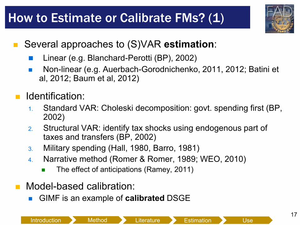
Several approaches to (S)VAR estimation:
Linear (e.g. Blanchard-Perotti (BP), 2002)
Non-linear (e.g. Auerbach-Gorodnichenko, 2011, 2012; Batini et al, 2012; Baum et al, 2012)
Identification: 1. Standard VAR: Choleski decomposition: govt. spending first (BP,
2002)
2. Structural VAR: identify tax shocks using endogenous part of taxes and transfers (BP, 2002)
3. Military spending (Hall, 1980, Barro, 1981)
4. Narrative method (Romer & Romer, 1989; WEO, 2010)
The effect of anticipations (Ramey, 2011)
Model-based calibration: GIMF is an example of calibrated DSGE
How to Estimate or Calibrate FMs? (1)
Introduction Literature Estimation Use Method
18
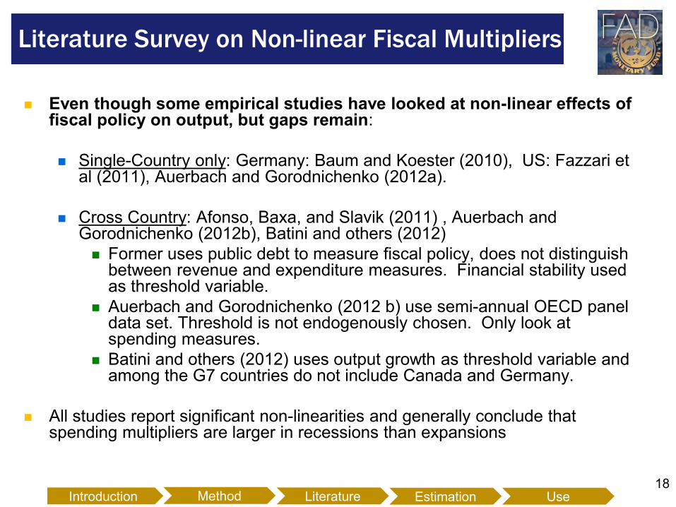
Even though some empirical studies have looked at non-linear effects of fiscal policy on output, but gaps remain:
Single-Country only: Germany: Baum and Koester (2010), US: Fazzari et al (2011), Auerbach and Gorodnichenko (2012a).
Cross Country: Afonso, Baxa, and Slavik (2011) , Auerbach and Gorodnichenko (2012b), Batini and others (2012)
Former uses public debt to measure fiscal policy, does not distinguish between revenue and expenditure measures. Financial stability used as threshold variable.
Auerbach and Gorodnichenko (2012 b) use semi-annual OECD panel data set. Threshold is not endogenously chosen. Only look at spending measures.
Batini and others (2012) uses output growth as threshold variable and among the G7 countries do not include Canada and Germany.
All studies report significant non-linearities and generally conclude that spending multipliers are larger in recessions than expansions
Literature Survey on Non-linear Fiscal Multipliers
Introduction Literature Estimation Use Method
19
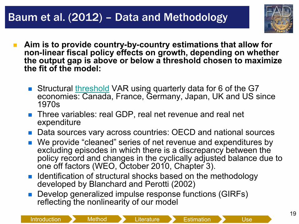
Aim is to provide country-by-country estimations that allow for non-linear fiscal policy effects on growth, depending on whether the output gap is above or below a threshold chosen to maximize the fit of the model:
Structural threshold VAR using quarterly data for 6 of the G7 economies: Canada, France, Germany, Japan, UK and US since 1970s
Three variables: real GDP, real net revenue and real net expenditure
Data sources vary across countries: OECD and national sources
We provide “cleaned” series of net revenue and expenditures by excluding episodes in which there is a discrepancy between the policy record and changes in the cyclically adjusted balance due to one off factors (WEO, October 2010, Chapter 3).
Identification of structural shocks based on the methodology developed by Blanchard and Perotti (2002)
Develop generalized impulse response functions (GIRFs) reflecting the nonlinearity of our model
Baum et al. (2012) – Data and Methodology
Introduction Literature Estimation Use Method
20
Fiscal Multipliers in
G-7 Economies
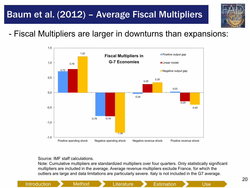
Baum et al. (2012) – Average Fiscal Multipliers
0,72
-0,78
-0,04
0,03
0,79
-0,79
0,29
-0,29
1,22
-1,34
0,35
-0,40
-1,5
-1,0
-0,5
0,0
0,5
1,0
1,5
Positive spending shock Negative spending shock Negative revenue shock Positive revenue shock
Positive output gap
Linear model
Negative output gap
Source: IMF staff calculations.
Note: Cumulative multipliers are standardized multipliers over four quarters. Only statistically significant
multipliers are included in the average. Average revenue multipliers exclude France, for which the
outliers are large and data limitations are particularly severe. Italy is not included in the G7 average.
- Fiscal Multipliers are larger in downturns than expansions:
Introduction Literature Estimation Use Method
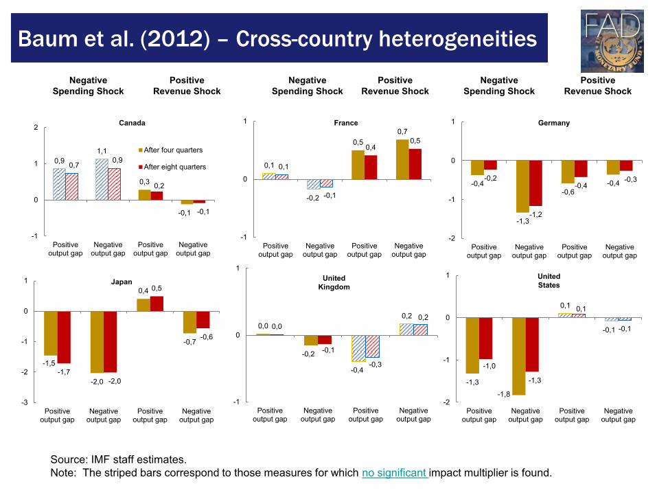
Baum et al. (2012) – Cross-country heterogeneities
Negative
Spending Shock
Positive
Revenue Shock
Negative
Spending Shock
Positive
Revenue Shock
Negative
Spending Shock
Positive
Revenue Shock
Canada
0,9
1,1
0,3
-0,1
0,7 0,9
0,2
-0,1
-1
0
1
2
Positiveoutput gap
Negativeoutput gap
Positiveoutput gap
Negativeoutput gap
After four quarters
After eight quarters 0,1
-0,2
0,5
0,7
0,1
-0,1
0,4 0,5
-1
0
1
Positiveoutput gap
Negativeoutput gap
Positiveoutput gap
Negativeoutput gap
France
-0,4
-1,3
-0,6
-0,4 -0,2
-1,2
-0,4 -0,3
-2
-1
0
1
Positiveoutput gap
Negativeoutput gap
Positiveoutput gap
Negativeoutput gap
Germany
-1,5
-2,0
0,4
-0,7
-1,7
-2,0
0,5
-0,6
-3
-2
-1
0
1
Positiveoutput gap
Negativeoutput gap
Positiveoutput gap
Negativeoutput gap
Japan
0,0
-0,2
-0,4
0,2
0,0
-0,1
-0,3
0,2
-1
0
1
Positiveoutput gap
Negativeoutput gap
Positiveoutput gap
Negativeoutput gap
United
Kingdom
-1,3
-1,8
0,1
-0,1
-1,0
-1,3
0,1
-0,1
-2
-1
0
1
Positiveoutput gap
Negativeoutput gap
Positiveoutput gap
Negativeoutput gap
United
States
Source: IMF staff estimates.
Note: The striped bars correspond to those measures for which no significant impact multiplier is found.
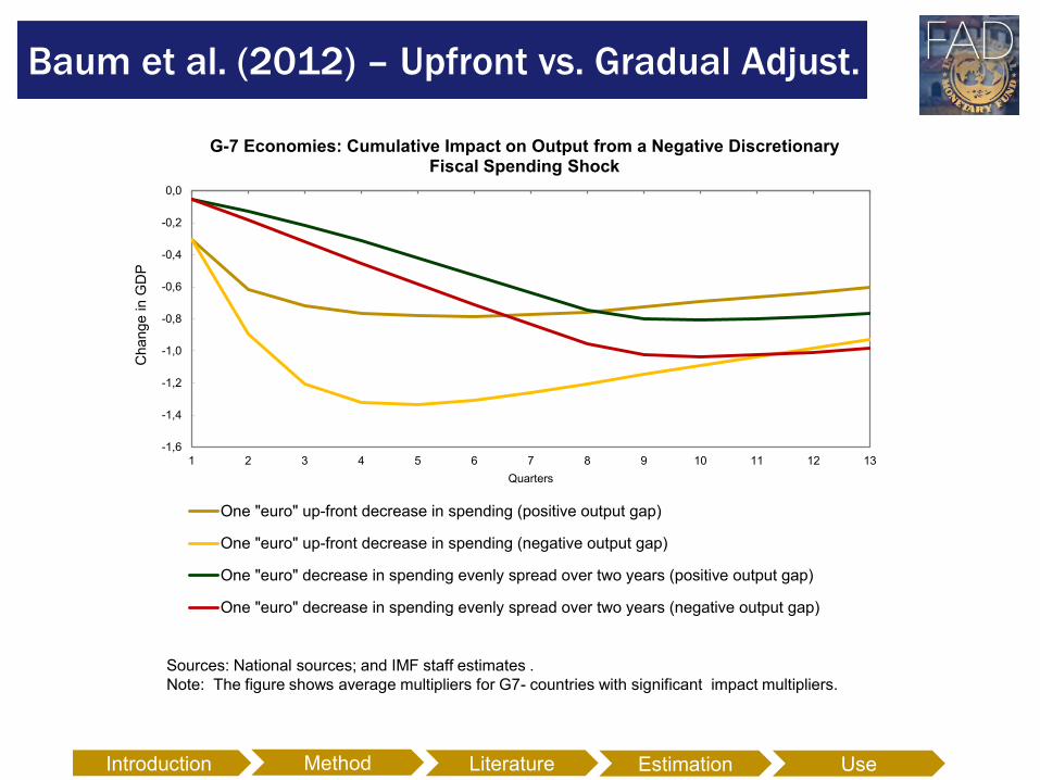
Baum et al. (2012) – Upfront vs. Gradual Adjust.
-1,6
-1,4
-1,2
-1,0
-0,8
-0,6
-0,4
-0,2
0,0
1 2 3 4 5 6 7 8 9 10 11 12 13
Change in G
DP
Quarters
One "euro" up-front decrease in spending (positive output gap)
One "euro" up-front decrease in spending (negative output gap)
One "euro" decrease in spending evenly spread over two years (positive output gap)
One "euro" decrease in spending evenly spread over two years (negative output gap)
G-7 Economies: Cumulative Impact on Output from a Negative Discretionary Fiscal Spending Shock
Sources: National sources; and IMF staff estimates .
Note: The figure shows average multipliers for G7- countries with significant impact multipliers.
Introduction Literature Estimation Use Method
23
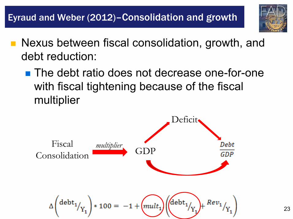
Nexus between fiscal consolidation, growth, and
debt reduction:
The debt ratio does not decrease one-for-one
with fiscal tightening because of the fiscal
multiplier
Eyraud and Weber (2012)–Consolidation and growth
Fiscal
Consolidation GDP
Deficit
multiplier
24
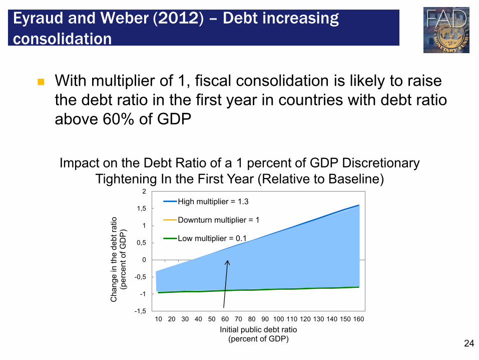
With multiplier of 1, fiscal consolidation is likely to raise
the debt ratio in the first year in countries with debt ratio
above 60% of GDP
Eyraud and Weber (2012) – Debt increasing
consolidation
Impact on the Debt Ratio of a 1 percent of GDP Discretionary
Tightening In the First Year (Relative to Baseline)
-1,5
-1
-0,5
0
0,5
1
1,5
2
10 20 30 40 50 60 70 80 90 100 110 120 130 140 150 160
Cha
nge
in t
he
de
bt ra
tio
(p
erc
en
t o
f G
DP
)
Initial public debt ratio (percent of GDP)
High multiplier = 1.3
Downturn multiplier = 1
Low multiplier = 0.1
25
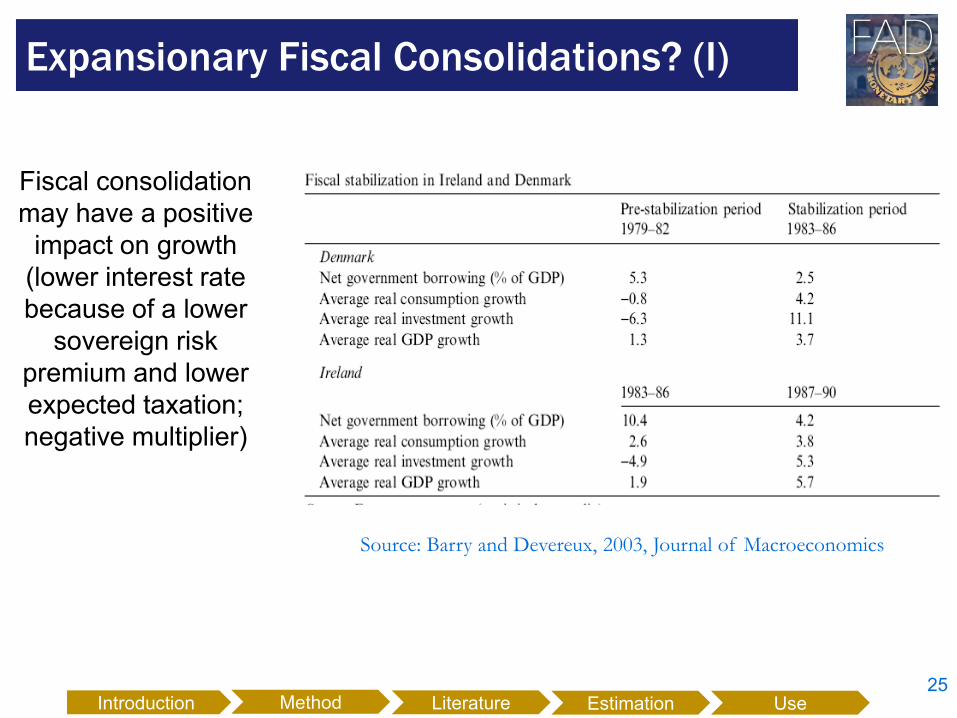
Expansionary Fiscal Consolidations? (I)
Source: Barry and Devereux, 2003, Journal of Macroeconomics
Fiscal consolidation
may have a positive
impact on growth
(lower interest rate
because of a lower
sovereign risk
premium and lower
expected taxation;
negative multiplier)
Introduction Literature Estimation Use Method
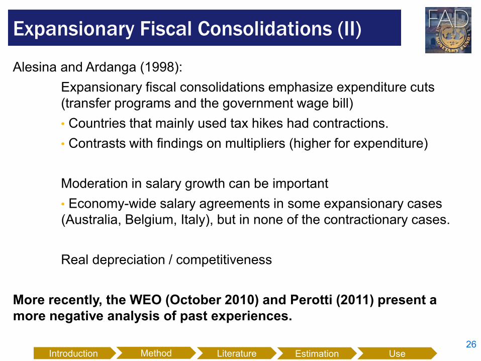
Alesina and Ardanga (1998):
Expansionary fiscal consolidations emphasize expenditure cuts
(transfer programs and the government wage bill)
• Countries that mainly used tax hikes had contractions.
• Contrasts with findings on multipliers (higher for expenditure)
Moderation in salary growth can be important
• Economy-wide salary agreements in some expansionary cases
(Australia, Belgium, Italy), but in none of the contractionary cases.
Real depreciation / competitiveness
More recently, the WEO (October 2010) and Perotti (2011) present a
more negative analysis of past experiences.
26
Expansionary Fiscal Consolidations (II)
Introduction Literature Estimation Use Method
27
Impact of fiscal policy on economic activity varies with the business
cycle.
Fiscal multipliers for the six economies analyzed are on average
larger in times of negative output gaps than when the output gap is
positive.
The value of multipliers differs noticeably across countries.
Spending shocks tend to have a larger effect on output when the
output gap is negative. The results are generally less conclusive
for revenue multipliers.
This heterogeneity of the multipliers calls for a tailored use of fiscal
policies and a country-by-country assessment of their effects.
The finding that the impact of fiscal policy on output depends on the
underlying state of the economy has important implications for the
choice between an upfront fiscal adjustment versus a more gradual
approach.
Baum et al. (2012) – Conclusions
Introduction Literature Estimation Use Method
28
If don’t have data, one option is to use some sort of categorized (“bucket”) approach
Idea: size of FM is related to a set of characteristics identified by the literature. For a given country, these combined characteristics suggest a possible multiplier range
The ranges could be based on: structural country characteristics that influence the
economy’s response to fiscal shocks in “normal times”
conjunctural/temporary characteristics (cyclical or policy-related phenomena) that make FMs deviate from “normal” levels
How to Estimate Multipliers? (2)
Introduction Literature Estimation Use Method
29
Several options to assess the growth impact of fiscal measures outside the financial programming framework:
Full-fledged model – needs resources and data; feasible for AEs, but not for many countries
Demand side approach on real sector – need to assess the effects on several items (private consumption and investment, exports and imports). Does not take into account second round effects
Fiscal multiplier in separate template – a possible approach for EMs and LICs
Incorporating FMs in Projections
Introduction Literature Estimation Use Method
30
Fiscal Multipliers are key inputs for assessment of the short-term macroeconomic impact of fiscal policy
The use of FMs in country teams is still heterogeneous.
Estimate or calibrate (model-based) fiscal multipliers explicitly may bring several benefits
Importance of the econometric procedure and identification for their empirical estimation.
The use of a multiplier template could complement the macro framework (but it is not a substitute for it or for the DSA)
Conclusion
Introduction Literature Estimation Use Method
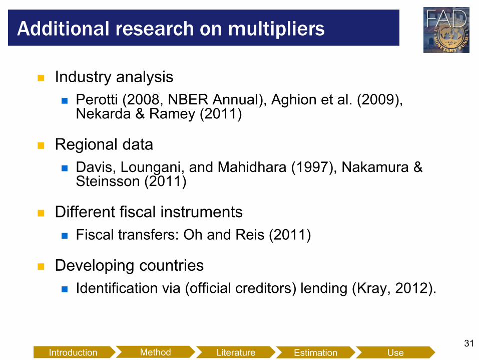
31
Industry analysis
Perotti (2008, NBER Annual), Aghion et al. (2009), Nekarda & Ramey (2011)
Regional data
Davis, Loungani, and Mahidhara (1997), Nakamura & Steinsson (2011)
Different fiscal instruments
Fiscal transfers: Oh and Reis (2011)
Developing countries
Identification via (official creditors) lending (Kray, 2012).
Additional research on multipliers
Introduction Literature Estimation Use Method

Thank you!
33
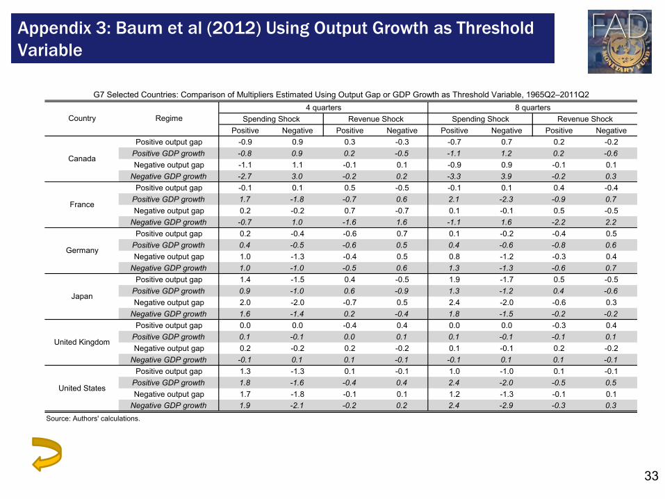
Appendix 3: Baum et al (2012) Using Output Growth as Threshold
Variable
Positive Negative Positive Negative Positive Negative Positive Negative
Positive output gap -0.9 0.9 0.3 -0.3 -0.7 0.7 0.2 -0.2
Positive GDP growth -0.8 0.9 0.2 -0.5 -1.1 1.2 0.2 -0.6
Negative output gap -1.1 1.1 -0.1 0.1 -0.9 0.9 -0.1 0.1
Negative GDP growth -2.7 3.0 -0.2 0.2 -3.3 3.9 -0.2 0.3
Positive output gap -0.1 0.1 0.5 -0.5 -0.1 0.1 0.4 -0.4
Positive GDP growth 1.7 -1.8 -0.7 0.6 2.1 -2.3 -0.9 0.7
Negative output gap 0.2 -0.2 0.7 -0.7 0.1 -0.1 0.5 -0.5
Negative GDP growth -0.7 1.0 -1.6 1.6 -1.1 1.6 -2.2 2.2
Positive output gap 0.2 -0.4 -0.6 0.7 0.1 -0.2 -0.4 0.5
Positive GDP growth 0.4 -0.5 -0.6 0.5 0.4 -0.6 -0.8 0.6
Negative output gap 1.0 -1.3 -0.4 0.5 0.8 -1.2 -0.3 0.4
Negative GDP growth 1.0 -1.0 -0.5 0.6 1.3 -1.3 -0.6 0.7
Positive output gap 1.4 -1.5 0.4 -0.5 1.9 -1.7 0.5 -0.5
Positive GDP growth 0.9 -1.0 0.6 -0.9 1.3 -1.2 0.4 -0.6
Negative output gap 2.0 -2.0 -0.7 0.5 2.4 -2.0 -0.6 0.3
Negative GDP growth 1.6 -1.4 0.2 -0.4 1.8 -1.5 -0.2 -0.2
Positive output gap 0.0 0.0 -0.4 0.4 0.0 0.0 -0.3 0.4
Positive GDP growth 0.1 -0.1 0.0 0.1 0.1 -0.1 -0.1 0.1
Negative output gap 0.2 -0.2 0.2 -0.2 0.1 -0.1 0.2 -0.2
Negative GDP growth -0.1 0.1 0.1 -0.1 -0.1 0.1 0.1 -0.1
Positive output gap 1.3 -1.3 0.1 -0.1 1.0 -1.0 0.1 -0.1
Positive GDP growth 1.8 -1.6 -0.4 0.4 2.4 -2.0 -0.5 0.5
Negative output gap 1.7 -1.8 -0.1 0.1 1.2 -1.3 -0.1 0.1
Negative GDP growth 1.9 -2.1 -0.2 0.2 2.4 -2.9 -0.3 0.3
Revenue ShockRegime
G7 Selected Countries: Comparison of Multipliers Estimated Using Output Gap or GDP Growth as Threshold Variable, 1965Q2–2011Q2
Source: Authors' calculations.
France
Germany
Japan
United States
United Kingdom
Country
Canada
4 quarters 8 quarters
Spending Shock Revenue Shock Spending Shock
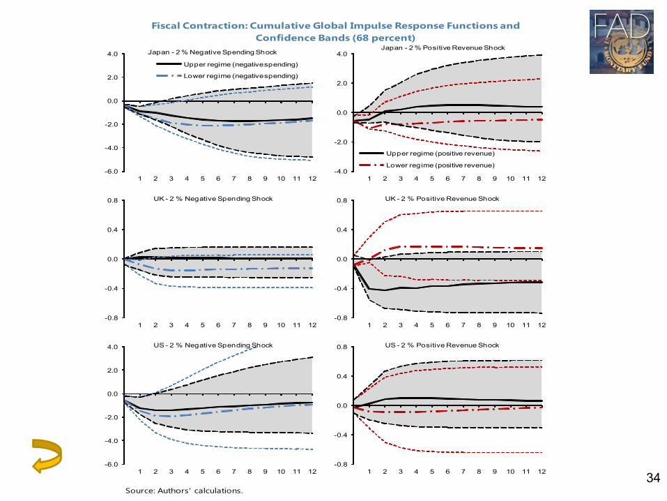
34
Fiscal Contraction: Cumulative Global Impulse Response Functions and
Confidence Bands (68 percent)
Source: Authors' calculations.
-6.0
-4.0
-2.0
0.0
2.0
4.0
1 2 3 4 5 6 7 8 9 10 11 12
Japan - 2 % Negative Spending Shock
Upper regime (negative spending)
Lower regime (negative spending)
-4.0
-2.0
0.0
2.0
4.0
1 2 3 4 5 6 7 8 9 10 11 12
Japan - 2 % Positive Revenue Shock
Upper regime (positive revenue)
Lower regime (positive revenue)
-0.8
-0.4
0.0
0.4
0.8
1 2 3 4 5 6 7 8 9 10 11 12
UK - 2 % Negative Spending Shock
-0.8
-0.4
0.0
0.4
0.8
1 2 3 4 5 6 7 8 9 10 11 12
UK - 2 % Positive Revenue Shock
-6.0
-4.0
-2.0
0.0
2.0
4.0
1 2 3 4 5 6 7 8 9 10 11 12
US - 2 % Negative Spending Shock
-0.8
-0.4
0.0
0.4
0.8
1 2 3 4 5 6 7 8 9 10 11 12
US - 2 % Positive Revenue Shock
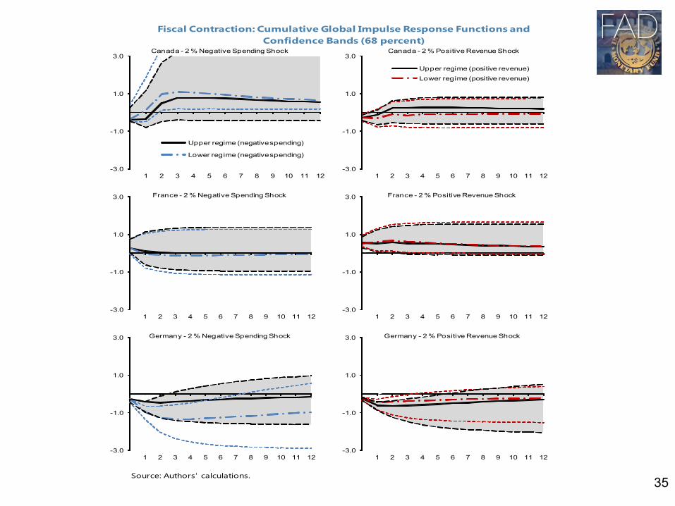
35
Fiscal Contraction: Cumulative Global Impulse Response Functions and
Confidence Bands (68 percent)
Source: Authors' calculations.
-3.0
-1.0
1.0
3.0
1 2 3 4 5 6 7 8 9 10 11 12
Canada - 2 % Negative Spending Shock
Upper regime (negative spending)
Lower regime (negative spending)
-3.0
-1.0
1.0
3.0
1 2 3 4 5 6 7 8 9 10 11 12
Canada - 2 % Positive Revenue Shock
Upper regime (positive revenue)
Lower regime (positive revenue)
-3.0
-1.0
1.0
3.0
1 2 3 4 5 6 7 8 9 10 11 12
France - 2 % Negative Spending Shock
-3.0
-1.0
1.0
3.0
1 2 3 4 5 6 7 8 9 10 11 12
France - 2 % Positive Revenue Shock
-3.0
-1.0
1.0
3.0
1 2 3 4 5 6 7 8 9 10 11 12
Germany - 2 % Negative Spending Shock
-3.0
-1.0
1.0
3.0
1 2 3 4 5 6 7 8 9 10 11 12
Germany - 2 % Positive Revenue Shock