fiscal policy and welfare in an endogenous growth model with … · 2018-05-30 · growth model...

Discussion Papers Collana di

E-papers del Dipartimento di Scienze Economiche – Università di Pisa

Davide Fiaschi

Fiscal policy and welfare in an endogenous growth model with heterogeneous endowments

Discussion Paper n. 18

2003

Discussion Paper n. 18, presentato: ottobre 2003 Indirizzi dell’Autore: Davide Fiaschi Dipartimento di scienze economiche, via Ridolfi 10, 56100 PISA fax: (39 +) 050 598040 e-mail : [email protected] © Davide Fiaschi La presente pubblicazione ottempera agli obblighi previsti dall’art. 1 del decreto legislativo luogotenenziale 31 agosto 1945, n. 660. Si prega di citare così: Davide Fiaschi, “Fiscal policy and welfare in an endogenous growth model with heterogeneous endowments”, Discussion Papers del Dipartimento di Scienze Economiche – Università di Pisa, n. 18 (http://www-dse.ec.unipi.it/ricerca/discussion-papers.htm).

Discussion Paper

n. 18

Davide Fiaschi

Fiscal policy and welfare in an endogenous

growth model with heterogeneous endowments

Abstract

This paper analyzes an endogenous growth model where agents havedifferent factor endowments and government finances public expendi-ture by imposing two flat-tax rates, one on capital income and one onlabor income. The main finding is that, in the absence of lump-sumredistributions, heterogeneity of endowments is crucial to determinethe optimal fiscal policy; in particular, taxing capital income is alwaysoptimal.

Classificazione JEL: H21; E13; D31; D3; H23.Keywords: Heterogeneous agents, Efficiency, Equity; Majority vot-ing.

2 D. Fiaschi

Contents

I. Introduction 3

II. The model 6II.A. Maximum growth . . . . . . . . . . . . . . . . . . . . 11

III.Normative analysis 12

III.A.Generalized Lorenz dominance and ranking of fiscalpolicies . . . . . . . . . . . . . . . . . . . . . . . . . . 14

III.B.Optimal fiscal policy . . . . . . . . . . . . . . . . . . 17

IV.Efficient fiscal policy 21

IV.A.Two agent economy . . . . . . . . . . . . . . . . . . . 23

V. Conclusions 24

A Optimal fiscal policy for agent i 25AA. Candidate solution . . . . . . . . . . . . . . . . . . . 27

AB. Check of candidate solution . . . . . . . . . . . . . . 28

B Derivation of equation (17) 30

C Proof of Proposition 10 31

D Leisure in utility function 32

E CES utility function 35EA. Maximum growth . . . . . . . . . . . . . . . . . . . . 38EB. Normative analysis . . . . . . . . . . . . . . . . . . . 38

EB.i. Efficient fiscal policy . . . . . . . . . . . . . . 42

Fiscal policy and welfare 3

I. Introduction

This paper analyses optimal taxation in a model of endogenousgrowth where agents have different endowments and government

finances public investment by means of two flat-tax rates, one onlabor income and the other on capital income.

It is a common finding in literature that optimal fiscal policy in-

volves zero capital tax. Judd (1985) shows that the optimal fiscalpolicy in the standard neoclassical growth model should not tax cap-

ital whenever other financing sources are available (see also Cham-ley (1986)) and Lucas (1990) extends this conclusion to endogenous

growth models with human capital (see also Jones, Manuelli andRossi (1997)). Finally Judd (1999) finds the same result in a growthmodel with public expenditure.1

However all these results are based on a representative agent

hypothesis2; when we consider agents with heterogeneous endow-ments, this has implications in terms of income distribution. The

fiscal regime where the tax rate on capital income is zero maximizesthe growth rate but damages agents who have a low endowment of

capital; then, even for a social planner indifferent to equity taxingincome capital would be optimal.3 The result holds provided that

more efficient redistributive instruments are not available.4

Welfare analysis is here based on the Lorenz dominance concept.5

Two paradigmatic fiscal policies are determined: the former max-imizing a Rawlsian welfare function (the social planner cares only

for the worst-off agent) and the latter the simple sum of all the in-

1Many contributions highlight the time inconsistency of this fiscal policy (see for exampleAlesina and Rodrik (1994)). However, as we will show, the optimal fiscal policy in our model istime-consistent because it also maximizes the output of every period (see Benhabib, Rustichiniand Velasco (2001)).

2Judd (1985) claims that his result also holds for an economy where individuals have differentfactor endowments.

3A social planner is considered to be indifferent to equity if she/he ranks alternative fiscalpolicies on the basis of the simple sum of individual utilities. This may be considered as ameasure of efficiency in an economy where agents have heterogeneous endowments.

4Stiglitz (1987) stresses the importance for welfare economics to study a world withoutdiscriminatory lump-sum taxes, given their difficult implementation.

5See Shorrocks and Foster (1987). This is the main difference with respect to Correia (1999).

4 D. Fiaschi

dividual utilities (a possible measure of efficiency). These two polar

cases are the bounds of the interval to which all socially optimalfiscal policies belong; intuitively the higher the social planner’s in-

equality aversion, the closer will be the welfare-maximizing fiscalpolicy to that which maximizes the Rawlsian welfare function.

The main result is that for any uneven distribution of initial fac-

tor endowments, the fiscal policy which maximizes growth does notbelong to the set of socially optimal fiscal policies. In other words,if initial endowments are heterogeneous, taxing capital income is

a necessary condition to maximize welfare. The distortion in theaccumulation of capital for poor agents is more than offset by the

increase in redistribution, at least for the fiscal policy where tax oncapital income is zero.

The key aspect of the model is to consider explicitely a growing

economy: Judd (1999), pag. 5, shows that a constant positive taxrate on capital income is equivalent to an explosive commodity tax

rate; the latter implies a explosive distortion and therefore it sug-gests not to tax capital income. However, to balance Governmentbudget, the lower is the tax on capital income the higher is the

tax on wage income. In turn, higher tax on wage income impliesa decrease in the initial consumption of all agents, whose effect is

also explosive in a growing economy.6 Moreover, the poor agentsare the more affected by this decrease in the initial consumption,

since they are relatively more endowed of labor. Therefore someagents, typically the poorest, get the maximum utility by a positive

tax on capital income, which implies a lower tax on wage income.This also explains because differently from Judd (1985), pag. 72,in our model workers prefer a positive tax on capital income in the

long-run.

The paper extends the literature on optimal taxation of capitalincome. Judd (1985) . From an analytical point of view the model is

close to Alesina and Rodrik (1994), but they consider taxation onlyon capital and do not focus their attention on the welfare effects

6The difference in the consumption paths corresponding to different levels of tax on wageincome is growing at the same rate of the growth rate of economy.


of different fiscal policies; the same consideration holds for Bertola

(1993). Judd (1999) analyzes the welfare property of the taxationof capital income in a model where public expenditure is productive

and optimally decided, but all agents have equal endowments, whichleads to the standard result of zero optimal taxation on capitalincome.7 Judd (1985) find the same result in a heterogeneous agents

economy, but as stated above, he considers an economy not growingin the long-run and this is crucial for the result.

It is worth to remark that the positive tax on capital income isnot the result of limiting our analysis to log-utility as in Lansing

(1999); in fact, Appendix E shows that the same finding is foundwhen agents have an intertemporal elasticity of substitution of con-

sumption different from 1.

Finally our result is a contribute to the literature on time-consistent

fiscal policy

We refer to Shorrocks and Foster (1987) for the (generalized)

Lorenz dominance concept; however, while there are many applica-tions of this concept in static welfare analysis, in a dynamic frame-

work, to our knowledge Karcher, Moyes and Trannoy (1995) is theonly contribution. Finally Correia (1999) is very close to our ap-

proach; however, she uses a different criterion (differential domi-nance instead of generalized Lorenz dominance) to rank alternativefiscal policies. In this respect, our results are more directly related

to the standard welfare analysis.

Appendix D extends the model to an economy with leisure.

The paper is organized as follow. In Section II. the basic model

is presented and it is determined the fiscal policy which maximizesthe growth rate; Section III. introduces the welfare analysis andcompares socially optimal equilibrium and maximizing growth fis-

cal policies. Finally, Section IV. shows how taxing capital income isalways optimal if agents have heterogeneous endowments. Conclu-

sions and references close the paper. Calculations and extensions

7Judd (1999), p. 16, claims that Jones, Manuelli and Rossi (1997)’s result of positive tax oncapital income in steady state is due to the exogenous rule adopted by government to decidepublic expenditure.

6 D. Fiaschi

are gathered in the Appendix.

II. The model

Assume that the aggregate production function is:8

Y = AKαG1−αL1−α, with 0 < α < 1, (1)

where Y is aggregate production, K is the capital, L is the labor, A

is a scale parameter and G is a factor provided by the government,which produces a positive externality on all the other productive

factors. G could be considered as productive services supplied bythe government to every firm.9

Assume G is financed with a balanced budget, such that

G = τrK + γwL, (2)

where τ and γ are two different flat taxes, respectively, on capitalincome and on labor income. Private factors receive their marginal

productivity; this implies that:10

r = αA1α [ατ + (1 − α) γ]

1−αα = r (τ, γ) and (3)

w = (1 − α)A1α [ατ + (1 − α) γ]

1−αα K = w (τ, γ)K. (4)

Notice that∂r

∂τ> 0,

∂r

∂γ> 0,

∂w

∂γ> 0 and

∂w

∂γ> 0, i.e. there is

a positive externality of public investment on factors’ income. By

substituting (2), (3) and (4) in (1), it follows that:

Y = A1α [ατ + (1 − α) γ]

1−αα K. (5)

Equation (5) makes it clear that this is an AK model, that is a

model where the marginal return on the cumulative factor remainsconstant, instead of decreasing, as the factor accumulates. More-

over, assume that factors cannot be subsidized and therefore τ andγ belong to the range [0, 1].

8The time index will always be omitted if this does not create confusion.9Y can be seen as the aggregation of N production functions yi = AG1−αk1−α

i l1−αi .

10For the sake of simplicity the total quantity of labor L is normalized to 1.


There are N consumers with different initial factor endowments.

Each consumer maximizes his intertemporal utility, taking as giventhe aggregate variable paths.

Let li be the labor endowment of agent i and ki her/his capitalendowment; therefore, her/his income will be expressed by

yi = ki [(1 − τ)r(τ, γ) + (1 − γ)w(τ, γ)σi] , (6)

where

σi =Kli

ki

, σi ∈ [0,+∞) (7)

is the relative factor endowment of the i-th agent.

The instantaneous utility function has a logarithmic form, suchthat every agent maximizes11

Ui =

∞∫

0

e−ρt log (ci) dt, (8)

where ρ is the intertemporal discount rate.

Given the time paths both of the tax rates and of the capitalaggregate stock,12 the maximization of Ui, subject to:

ki = ki [(1 − τ)r(τ, γ) + (1 − γ)w(τ, γ)σi] − ci (9)

yields the following optimal consumption path:

ci

ci= (1 − τ)r(τ, γ)− ρ. (10)

Suppose that fiscal policy is constant over time (like Alesina andRodrik (1994)).13 Then it is possible to demonstrate that equation

11See Appendix E for an extension of analysis to the case of CES utility function Ui =c1−µ

i−1

1−µ,

where 1µ

is the intertemporal elasticity of substitution of consumption.12Interactions among individuals actually occur only through the decisions on τ and γ because

r and w are independent of capital stock (see (3) and (4)).13This is not source of limitation of the analysis; Appendix A contains a proof that the

optimal fiscal policy is actually constant over time. However, the more general procedure ofsolution appears very tedious and not very intuitive from an economic point of view.

8 D. Fiaschi

(10) is also the growth rate of K and ki along the individual optimal

path,14 such that

ci

ci=ki

ki

=K

K= (1 − τ)r(τ, γ)− ρ = η (τ, γ) . (11)

Therefore η (τ, γ) represents the steady state growth rate as afunction of the sequence of tax rates on capital income and laborincome; moreover (7) and (11) highlight the fact that the relative

factor endowment σ of every agent does not change over time.By (9), (10) and (11) the instantaneous level of consumption

along the optimal path can be calculated, that is:

ci = [(1 − γ)w(τ, γ)σi + ρ] ki. (12)

The linear relationship between ci and ki causes aggregate saving

to be independent of endowment distributions and therefore fiscalpolicy affects the dynamics of the economy just by changing the

price of factors; this property directly derives from the assumptionof homothetic preferences.15

The optimal fiscal policy for the i-th agent solves the followingproblem:

max{τ,γ}∞t=0

Ui =

∞∫

0

e−ρt log (ci) dt (P1)

s.t.

ci = [(1 − γ)w(τ, γ)σi + ρ] ki

ki

ki

=K

K= η (τ, γ)

τ, γ ∈ [0, 1] .

We stress that the two tax rates are not assumed to be constant;the current value Hamiltonian for problem (P1) is given by16

H = ln {ki [(1 − γ)w (τ, γ)σi + ρ]} + λki [(1 − τ) r (τ, γ) − ρ] .

14This is a standard result of AK growth models, where economy jumps instantaneously toits steady state (see Barro and Sala-I-Martin (1999)).

15For a similar argument see Correia (1999).16We ignore the constraints on τ and γ in the formulation of the Hamiltonian, but we will

take them into account in the discussion of the results.


The following are necessary and sufficient conditions for the opti-

mum:17

∂H

∂τ= 0; (13)

∂H

∂γ= 0; (14)

λ = ρλ− ∂H

∂ki

; (15)

limt→∞

e−ρtλki = 0. (16)

From (13), (14) and (15), it follows that:18

τ =(1 − α) (1 − γ)

α. (17)

Equation (17) shows that there is a linear relation between the in-dividual optimal tax rates; this will be fundamental in determining

the politico-economic equilibrium because it allows a generalizationof the median-voter theorem to be applied.

Equation (17) represents a static optimal condition; indeed, itcan be verified that to maximize the net total output with respect

to τ and γ, that is

Y −G = A1αK{

[ατ + (1 − α) γ]1−α

α − [ατ + (1 − α) γ]1α

}

, (18)

tax rates have to satisfy equation (17). From the latter result we

can conclude that every fiscal policy, and therefore also the optimalfiscal policy of i-th agent, satisfying equation (17) is not subject

to the time inconsistency problem (see Benhabib, Rustichini andVelasco (2001)).

The optimal tax rate on capital income for agent i follows by

17Under the usual hypothesis of concavity of the hamiltonian function with respect to stateand control variables.

18See Appendix B.

10 D. Fiaschi

substituting (17) in (13):19

τi = max

[

0,ρ (σi − 1)

rσi

]

, (19)

where r = αA1α (1 − α)

1−αα is the value of r when (17) holds. We

are implicitly assuming that r > ρ, which represents a necessarycondition to have a positive steady state growth rate.

Therefore the optimal tax on labor income will be:

γi = min

[

1, 1 −(

α

1 − α

)(

ρ (σi − 1)

rσi

)]

. (20)

The optimal tax rate on capital income for the i-th individual

τi will be zero if her/his relative factor endowments is less thanor equal to 1 and positive for values greater than 1. Moreover, τiis constant over time, such that the optimal fiscal policy impliesconstant tax rates. The individual optimal tax rate on a factor is

inversely proportional to her/his relative endowment of that factor;for example if her/his relative capital endowment falls (i.e. σi in-creases), then the optimal tax rate on capital income increases (see

(19)). Moreover, provided that equation (17) holds, w and r areindependent of τ and γ.

To examine this point in greater depth, assume constant taxrates (this property holds for each agent’s optimal fiscal policy, see

(19)). Solving the integral in (P1) yields the following expressionfor individual utility:

U (σi, τ, γ) =1

ρ

{

log{

k0i [(1 − γ)w (τ, γ)σi + ρ]

}

+(1 − τ) r (τ, γ)− ρ

ρ

}

.

(21)

The first term of (21) is consumption at time 0 (denote thisas level effect), while the second term is proportional to steady

19From (65), (11) and (71) it follows that

ρ

τrσi + ρ=

1

σi

.

Solving for τ we obtain equation (19).


state growth rate η (denote this as growth effect). The individual

optimal fiscal policy is determined by the trade-off between thesetwo effects; maximizing the growth rate, on the contrary, amounts to

considering only the second effect. If equation (17) holds, the growtheffect and the level effect are, respectively, negatively and positivelyrelated to τ . The level effect positively depends on σ. This explains

the relationship between individual preferences on fiscal policy andrelative factor endowments given by (19).

II.A. Maximum growth

To understand how fiscal policy affects the steady state growthrate expressed by (11), consider equation (12), that shows how the

ratio between ci and ki varies along the balanced growth path asa function of the tax rates. Notice that the higher the tax rate on

capital income, the higher is the instantaneous level of consumptionfor a given ki; this, in turn, implies a lower investment rate andtherefore a lower growth rate (see Bertola (1993)). The following

Proposition states the fiscal policy which maximizes the growth rate:

Proposition 1 The fiscal policy which maximizes the growth rateη (τ, γ) is given by (τ ∗, γ∗) = (0, 1).

Proof. Consider the derivative of equation (11) with respect to

τ and γ. Since∂η (τ, γ)

∂τ> 0 ⇔ τ < (1 − α) (1 − γ) ,

∂η (τ, γ)

∂γ>

0 ∀ (τ, γ) and τ, γ ∈ [0, 1], then the fiscal policy which maximizesgrowth is given by (τ ∗, γ∗) = (0, 1).

The intuition is straightforward: the growth rate of output de-pends on the accumulation of capital and, because the saving rate

positively depends on its return, taxation of capital income reducesthe incentives to accumulate. This does not hold for labor because

it has an inelastic supply. Allowing for leisure, the tax rate on laborincome which maximizes the steady state growth rate γ∗ will be

equal to π < 1, where π is inversely proportional to the elasticity ofsubstitution between leisure and working time; more details on thiscase are reported in Appendix D.

12 D. Fiaschi

Finally, we note that it is the accumulation of capital that gen-

erates growth, while the level of G affects only the production level;this rules out the possibility that, in order to maximize the growth

rate, capital income has to be taxed.

For simplicity and because this is not a source of limitation ofthe analysis, in the following assume that every agent has the same

labor endowment, such that a difference in σ reflects different capitalendowments, that is:

li = l =1

N∀i ∈ {1, ..., N} . (22)

This assumption makes σ inversely related to the level of indi-

vidual income, so that all results can be also interpreted in termsof income.

Moreover, to avoid trivial results in the following assume, if not

otherwise specified, that σ is uneven distributed, that is:

∃i, j ∈ {1, ..., N} with i 6= j such that σi 6= σj. (23)

III. Normative analysis

The aim of this section is to rank consumption paths in welfareterms. In this contest the distribution of capital will be crucial

to determine the optimal fiscal policy. Heuristically if every agenthas the same capital endowment, then σ = 1 and the fiscal policyτ = 0 and γ = 1, which maximizes steady state growth rate, will

maximize welfare as well. Thus in this representative agent economythere would be not any trade-off between equity and efficiency (this

is the Judd (1999)’s finding).20

However this result does not hold any more if agents have hetero-

geneous endowments; in particular, on the condition that lump-sumredistributions are not available, we will demonstrate that thereis no more a perfect correspondence between fiscal policies which

20Notice that if assumption (22) does not hold, σi = 1∀i does not imply all agents’ endow-ments are equal.


maximize welfare and steady state growth rate.21

In the economy there are many Pareto optima; indeed the opti-mal fiscal policy of every agent is a Pareto optimal allocation, but

these are not the only ones. In particular, since the individual utilityfunction is concave,22 the set of Pareto optima is an interval whose

bounds are for every tax rate, respectively, the optimal fiscal policyof the agents with the highest and the smallest value of σ. Thus thefiscal policy which maximizes the growth rate is not the optimum,

but only one among all the possible Pareto optima.The following analysis is focused on all combinations of (τ, γ),

constant over time, belonging to the line segment (17).23 Giventhese assumptions, the indirect utility of agent i becomes:

U (σi, τ) =1

ρ

{

log{

k0i [τ rσi + ρ]

}

+(1 − τ) r − ρ

ρ

}

.

Since every fiscal policy can be expressed as a function of only taxrate of capital income τ , for the sake of simplicity in the followingwe will refer only to this variable to indicate fiscal policy, when this

is not source of confusion.

To rank in welfare terms the elements of the set of Pareto optimawe need to postulate a social welfare function. Assume that thewelfare function is additive-separable, that is:

W =N∑

j=1

φ(

U (σj, τ))

.

The social planner’s inequality aversion is expressed by the form

of φ (·); for example, if she/he were indifferent to inequality, φ (·)21We do not discuss the case of redistribution of initial endowment (i.e. confiscation of

capital) leading to a uniform distribution of factors among agents, due to of both its possibleintertemporal inconsistency (see Alesina and Rodrik (1994)) and its difficult implementation(see Lucas (1990)).

22This can be checked by (21), using equation (17).23This is not a source of limitation for the analysis because relationship (17) between the

two optimal tax rates does not depend on agents’ endowments. Moreover, we have shown thatalso individual optimal fiscal policy provides for constant tax rates. Finally, it will be shownthat relationship (17) is always satisfied when the social planner maximizes the simple sum ofindividual utilities.

14 D. Fiaschi

would be linear in its arguments. In an economy with heterogeneous

endowments the latter case is a natural candidate for representingan efficient index of fiscal policy.

Finally, we define the optimal fiscal policy:

Definition 2 (Optimal fiscal policy) Let(

τW , γW)

be the opti-mal fiscal policy, where

τW = arg maxτ∈[0,1]

[

N∑

j=1

φ(

U (σj, τ))

]

; (24)

γW = 1 −(

α

1 − α

)

τW . (25)

III.A. Generalized Lorenz dominance and ranking of fis-

cal policies

A very useful concept in welfare analysis is the (generalized)Lorenz dominance; the latter allows to rank alternative fiscal poli-

cies in welfare terms. In particular, Shorrocks and Foster (1987)state the following Theorem on the relationship between additive

separable welfare function and (generalized) Lorenz dominance24:

Theorem 3 Assume that φ′ (·) ≥ 0 and φ′′ (·) ≤ 0 and let U τq

=[

U (σ1, τq) , ..., U (σN , τ

q)]

be a utility vector of length N, whose ele-ments are ranked in an increasing order, i.e. U (σ1, τ

q) ≤ U (σ2, τq) ≤

... ≤ U (σN , τq), then

GLτA

(p) ≥ GLτB

(p) , ∀p ∈ [0, 1] ⇔N∑

j=1

φ(

U(

σj, τA))

≥N∑

j=1

φ(

U(

σj, τB))

,

where GLτq

(p) =∑S

j=1 U(σj ,τq)

N, q = A,B, p =

S

Nand S = 1, ..., N .

24In general Shorrocks and Foster’s Theorem refers to a ranking of alternative (income)vectors. Since balanced consumption path is a matrix (the set of consumption paths of allagents) and not a vector, an aggregation is necessary. We use an aggregate index for theconsumption path of each agent, her/his intertemporal utility U . Other approaches are possible;see for example Karcher, Moyes and Trannoy (1995).


The GLτ (p) is the (generalized) Lorenz curve and U τA

is saidto dominate U τB

according to the Lorenz dominance principle; re-

fer to Shorrocks and Foster (1987) for the proof. If GLτA

(p) werenot always above GLτB

(p), then a univocal conclusion could not be

reached without imposing other constraints on the form of φ (·) (seeDardanoni and Lambert (1988)).

The definition of efficient fiscal policy in heterogeneous agent

economies is controversial; according to our approach we measurethe efficiency of a fiscal policy by the simple sum of individual util-

ities. In the following we give the definition of efficiency improvingfiscal policy:25

Definition 4 (Efficiency improving fiscal policy) Let τA andτB be two fiscal policies; then τA is more efficient than τB if GLτA

(1) >

GLτB

(1).

Finally, as regards equity the following definition states the fiscalpolicies that present an efficiency-equity trade-off:

Definition 5 (Efficiency-equity trade-off fiscal policy) LetτA and τB be two fiscal policies; then τA is more equitable than τB

and τB is more efficient than τA if ∃p ∈ (0, 1) such that ∀p ∈ [0, p]GLτA

(p) ≥ GLτB

(p) and ∀p ∈ (p, 1] GLτA

(p) ≤ GLτB

(p).

The intuition is straightforward: if the change from fiscal policyτB to τA causes an upward movement in the part of the Lorenzcurve nearer to the origin and a downward movement in the other

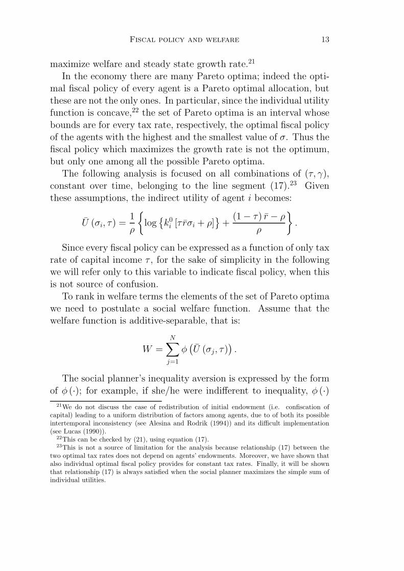
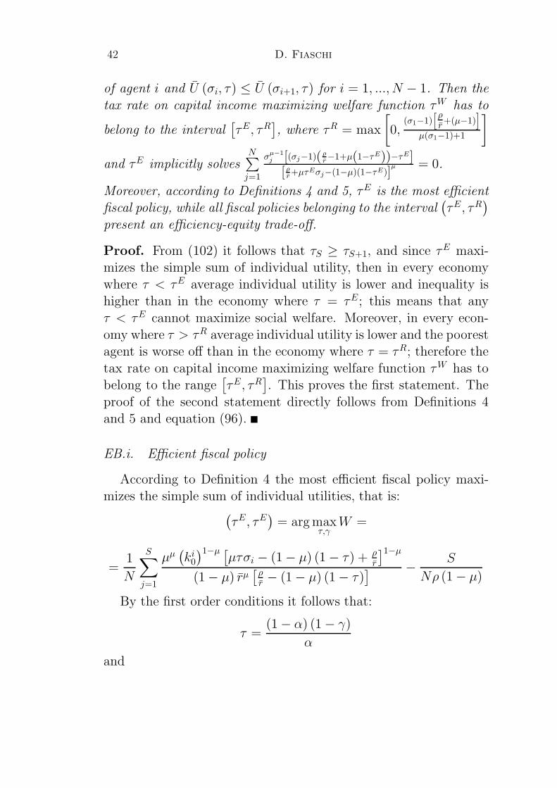
part, then fiscal policy τA is related to a lower inequality but a lowerefficiency than τB. Figure 1 shows this case.

FIGURE 1 HERE

In Figure 1 τB is an efficiency improving policy with respect to

τA (the sum of individual utilities increases), but it also implies a

25Our definition of efficient improving fiscal policy is different from that used by Correia(1999); in fact we refer to the sum of individual utilities, while Correia (1999) considers theutility related to average endowment. In the latter case the most efficient fiscal policy is alwaysτ = 0, because average endowment corresponds to σ = 1.

16 D. Fiaschi

greater inequality (the poor agent has a lower (relative) utility).

Thus the change from fiscal policy τB to τA implies an efficiency-equity trade-off.

In our framework the generalized Lorenz curve is defined as (seeTheorem 3):

GLτ (p) =

S∑

j=1

U (σj, τ)

N=

=

S∑

j=1

[

ln (τ rσj + ρ) k0j

]

+ S[

(1−τ)r−ρ

ρ

]

ρN

for S = 1, ..., N ; the derivative of GLτ (p) with respect to τ shows

how fiscal policy affects the Lorenz curve:

∂GLτ (p)

∂τ=

(

1

ρN

)

[

S∑

j=1

rσj

τ rσj + ρ− Sr

ρ

]

. (26)

Theorem 3 can be applied only if ∂GLτ (p)∂τ

does not change its signfor S = 1, ..., N .

From equation (26) it follows that:

if

S∑

j=1

σj

S= µS

σ > 1 ⇒ ∂GLτ (p)

∂τ

∣

∣

∣

∣

τ=0

> 0 S = 1, ..., N, (27)

where µSσ is the mean of distribution of σ of the first S agents. The

condition expressed by (27) is intuitive: since agents with a σ no

greater than 1 prefer τ = 0 (see (19)), for every S = 1, ..., N theLorenz curve shifts up or down as τ becomes greater than 0 depend-

ing on the mean of the σ of the first S agents being, respectively,

greater or smaller than 1. Therefore from Definition 4 if ∂GLτ (1)∂τ

∣

∣

∣

τ=0were greater than 0 then τ = 0 could not be the most efficient fiscalpolicy.


III.B. Optimal fiscal policy

This section characterizes the set of all possible optimal fiscalpolicies.

Firstly, we defines two extreme fiscal policies, one maximizing a

Rawlsian welfare function, corresponding to a social planner inter-ested only in the worst-off agent’s utility, and one maximizing the

simple sum of individual utilities, corresponding to a social plannerthat aims only at efficiency. Secondly, we show how within thisrange there are all candidate optimal fiscal policies; the effectively

optimal one will depend on the social planner’s inequality aversion.

According to Rawls’ principle the welfare of an economy is repre-sented by the utility of the worst-off; this means that social welfare

is given by the value of the Lorenz curve corresponding to abscissa1N

. The following Proposition states the optimal fiscal policy of a

Rawlsian social planner:

Proposition 6 Let(

τR, γR)

be the optimal fiscal policy when the

social planner has Rawlsian preferences. Then τR maximizes GLτ(

1N

)

,that is:

τR = arg maxτ∈[0,1]

[

GLτ

(

1

N

)]

= max

[

0,ρ (σ1 − 1)

rσ1

]

(28)

and

γR = min

[

1, 1 −(

α

1 − α

)(

ρ (σ1 − 1)

rσ1

)]

. (29)

Proof. To prove (28) it is sufficient to note that U (σ1, τ) ≤U (σ2, τ) ≤ ... ≤ U (σN , τ), while γR is derived from (17).

On the contrary, if efficiency is the only goal of the social planner,

social welfare is given by the value of the Lorenz curves correspond-ing to abscissa 1. The following Proposition states the optimal fiscal

policy in this case:

Proposition 7 Let(

τE, γE)

be the optimal fiscal policy when ef-ficiency is the only goal of social planner. Then τE maximizes

18 D. Fiaschi

GLτ (1), that is:∂GLτ (1)

∂τ

∣

∣

∣

∣

τ=τE

= 0 (30)

and

γE = 1 −(

α

1 − α

)

τE. (31)

Proof. The proof of (30) is given by the definition of efficiency

improving fiscal policy (see Definition 4), while γE is derived from(17).

Proposition 7 yields the following condition:

∂GLτ (1)

∂τ

∣

∣

∣

∣

τ=τE

= 0 ⇔N∑

j=1

σj

τE rσj + ρ=N

ρ(32)

From condition (32) it follows that τR ≥ τE.26 This suggeststhat τW has to belong to the interval

[

τE, τR]

and the higher is thesocial planner’s inequality aversion the closer is τW to τR. With

respect to this point, note that since σ1 ≥ σ1 ≥ ... ≥ σN then:

S∑

j=1

σj

τ rσj + ρ

S≥

S+1∑

j=1

σj

τ rσj + ρ

S + 1for S = 1, ..., N − 1 and ∀τ ∈ [0, 1] .

(33)

Given that τE has to satisfy the following equality:

N∑

j=1

σj

τE rσj + ρ− N

ρ= 0,

it follows that:

∂GLτ (p)

∂τ

∣

∣

∣

∣

τ=τE

=S∑

j=1

σj

τE rσj + ρ− N

ρ≥ 0 for S = 1, ..., N − 1.

26Note that σ1

τ rσ1+ρ≥ σj

τ rσj+ρ∀j = 2, ..., N and ∀τ ∈ [0, 1], hence

N∑

j=1

σj

τRrσj+ρ≤ N

ρand

therefore τR ≥ τE .


This means that the Lorenz curve corresponding to τE is every-where increasing in τE, except for p = 1; in other words an increase

in τE causes a decrease in income inequality (but also a decrease inaverage utility).

Let τS be the level of tax rate that, if increased, would leave

GLτ (p) unchanged (remember that p = SN

), that is:

∂GLτ (p)

∂τ

∣

∣

∣

∣

τ=τS

= 0.

From (33) it follows that vector {τS}NS=1 is ranked in decreas-

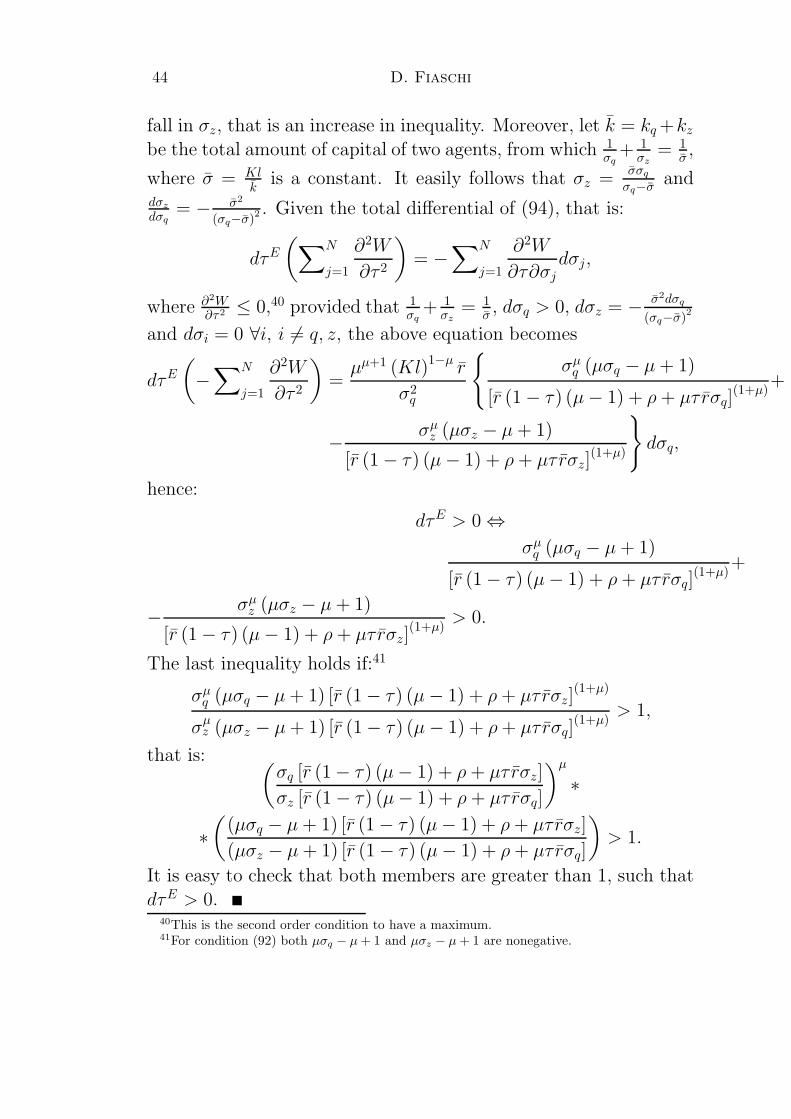
ing order, i.e. τS ≥ τS+1, such that τ1 = τR and τN = τE (seePropositions 6 and 7).

We see that an increase in τ causes an upward movement of

the part of GLτS on the left with respect to the point of abscissap = S

Nand a downward movement of the part on the right (here the

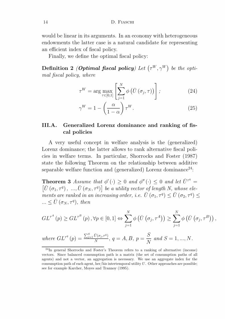
application of Definition 5 of efficiency-equity trade-off fiscal policyto τS is straightforward). Figure 2 shows two Lorenz curves, one

corresponding to τS and another one corresponding to τ > τS; theyhave to cross only in a single point.

FIGURE 2 HERE

Each τ < τE = τN never maximizes social welfare because suchan increase causes an upward movement of the whole GLτ (p) curve

and therefore a welfare gain (see Theorem 3).For every τ > τN an increase in tax rate causes only the left part

of the GLτ (p) curve to shift up, while the right part shifts down;

this means that the poorest agents increase their welfare, while allthe others experience reduced status; moreover, for every τ > τNan increase in τ leads to a fall in the average social welfare. Sincethe higher is τ the smaller is the number of agents preferring a rise

in τ , then if τ were increased over τ1 also the worst-off agent wouldworsen her/his status; this implies that τ1 = τR.

This confirms the previous intuition that τW ∈[

τE, τR]

and thatthe level of tax rate maximizing social welfare will positively dependon the social planner’s inequality aversion.

20 D. Fiaschi

The following Proposition summarizes the results:

Proposition 8 Let W =N∑

j=1

φ(

U (σj, τ))

be the social welfare func-

tion, where φ′ ≥ 0, φ′′ ≤ 0, U (σi, τ) is the intertemporal utility of

agent i and U (σi, τ) ≤ U (σi+1, τ) for i = 1, ..., N − 1. Then thetax rate on capital income maximizing welfare function τW has to

belong to the interval[

τE, τR]

, where τR = max[

0, ρ(σ1−1)rσ1

]

and τE

implicitly solvesN∑

j=1

σj

τE rσj+ρ= N

ρ.

Moreover, according to Definitions 4 and 5, τE is the most effi-cient fiscal policy, while all the other fiscal policies belonging to theinterval

(

τE, τR)

present an efficiency-equity trade-off.

Proof. From equation (33) it follows that τS ≥ τS+1, and since τE

maximizes the simple sum of individual utilities, then in every econ-omy where τ < τE average individual utility is lower and inequality

is higher than in the economy where τ = τE; this means that noτ < τE can maximize social welfare W . Moreover in every economy

where τ > τR average individual utility is lower and the utility ofthe poorest agent is less than in the economy where τ = τR; there-

fore τW has to belong to the interval[

τE, τR]

. This proves the firststatement. The proof of the second statement directly follows fromDefinitions 4 and 5 and from equation (33).

Moreover:

Remark 9 The efficient fiscal policy τE dominates according to theLorenz dominance principle every fiscal policy τ < τE.

Proof. From equation (33) and since τE maximizes the sum of

individual utilities, a decrease in τE causes a downward movementof the whole Lorenz curve, which holds for every τ < τE. This

completes the proof.The next section analyzes thoroughly the case of efficient fiscal

policy. This case is particularly interesting because τE is both thelower bound of the set of possible optimal fiscal policies and themost efficient fiscal policy (see Remark 9).


IV. Efficient fiscal policy

In this section we show that taxing capital income is always op-timal if agents have heterogeneous endowments. According to Def-

inition 4 the most efficient fiscal policy maximizes the simple sumof individual utilities, that is:

(

τE, γE)

= arg maxτ,γ∈[0,1]2

W =

=

lnN∏

j=1

k0j [(1 − γ)w (τ, γ)σi + ρ] +N

(1 − τ) r (τ, γ)− ρ

ρ

ρ.

By the first order conditions it follows that:

τ =(1 − α) (1 − γ)

α.

This result supports the previous choice to focus only on the fiscalpolicies belonging to the straight line given by (17); substituting

(17) in the first order conditions of (IV.) and solving for γ yields:27

N∑

i=1

σi

τE rσi + ρ

N=

1

ρ. (34)

Setting τE = 0 in (34) yields a sufficient condition to have τE = 0,

that is:28

µσ =

∑Nj=1 σj

N= 1. (35)

It can be demonstrated that µσ = 1 implies σi = 1 ∀i;29 therefore,provided that condition (35) holds, since every agent has the same

relative endowment σ = 1 and prefers τ = 0, it follows that τE =τW = 0. This case corresponds to the representative agent economy

and the result coincides with Judd’s (1999) finding.

27The logarithmic form of utility function prevents fiscal policy maximizing growth frommaximizing social welfare if at least one agent has no quantity of capital.

28Condition (35) could also be derived from (27).29See Appendix C.

22 D. Fiaschi

The mean of the σ distribution proves a crucial parameter; intu-

itively the greater the mean of σ, the higher is the number of agentspreferring high tax rate on capital income. Moreover, σi = 1 ∀i is

also the allocation of endowments minimizing µσ, which suggeststhat if µσ > 1 then τE > 0 (that is (35) is not only a sufficient, butalso necessary condition to have τE = 0). The following Proposition

confirms this intuition:

Proposition 10 The most efficient fiscal policy (or the optimal fis-cal policy when the social planner is indifferent to inequality) in-

volves a positive tax rate on capital income, but the case of evendistribution of individual endowments (i.e. the representative agenteconomy), that is:

τE =

{

0 if σi = 1 ∀iψ > 0 if ∃i such that σi 6= 1

Proof. See Appendix C.

The intuition is straightforward: given an unequal distributionof resources, the poor agents (i.e. laborers) have such a low level of

consumption that they benefit from trading off lower growth withhigher initial levels of consumption. In fact, a positive taxation oncapital income means a greater share of total income is allocated

to labor, which implies a higher consumption in the initial periodsfor all agents, but a lower growth rate. The richest agents have a

loss from this consumption reallocation, but the concave form ofindividual utility function always makes the latter lower than the

gain of the poor agents.30 Appendix E extends this result to aneconomy where agents have a CES utility function.

In the optimal taxation literature there exists a standard result(for a representative agent economy), that states that the optimal

30Here the difference with the definition of efficiency proposed by Correia (1999) is crucial:she considers the utility of the agent with average endowment as a measure of efficiency offiscal policy, but this implies that concavity of the individual utility function does not matter.In other words, the distribution of endowments would not affect the efficiency of fiscal policy.Adopting the definition of efficiency proposed by Correia (1999), in this economy, independentof endowment distribution, the most efficient fiscal policy would be always to tax zero capitalincome.


tax rate on capital income is zero (e.g. Judd (1999)); Proposition 10

states that for a heterogeneous agents’ economy exactly the oppositeholds.

IV.A. Two agent economy

This section analyzes a simple example, a two agent economy

(e.g. a capitalist and a worker like in Judd (1985)). Denote as theiso-tax rate curve the set of all the pairs (σ1, σ2) that imply the same

level of τE; from (34) this can be expressed as:

σ2 = −ρ[

σ1

(

2τE r − ρ)

+ 2ρ

2τE rσ1 (τE r − ρ) + ρ (2τE r − ρ)

]

.

If τE = 0 the slope of iso-tax rate curve is always equal to −1and therefore the iso-tax rate curve is a straight line, while if τE > 0the iso-tax rate curve is concave. Since all the feasible pairs (σ1, σ2)

have to belong to the curve σ2 = σ1

2σ1−1,31 it is easy to verify that

µσ = 1 ⇔ σ1 = σ2 = 1. Moreover, for any σ1, σ2 6= 1 we have

τE > 0 and only if σ1 = σ2 = 1, then τE = 0 (these results are justan application of Proposition 10).

Finally, from (34) with a little algebra it follows that32

τE =(ρ

r

)

[√

5 − 4

µσ

− 1

]

,

which highlights the positive relationship between τE and the mean

of σ. It is easy to show that µσ increases as distribution becomesmore unequal.33

Figure 3 shows in (σ1, σ2) space the resource constraint σ2 =σ1

2·σ1−1 and two iso-tax rate curves.

31To see this, consider that the resource constraint implies 1σ1

+ 1σ2

= 2, hence σ2 = σ1

2σ1−1 .32Mean and variance of distribution of σ have a positive relationship if σ1 > 1; in particular

varσ = µσ

[

(σ1−1)2

2σ1−1

]

.

33By definiton of mean µσ =(

12

)

[

σ1 + σ1

2σ1−1

]

=σ2

1

2σ1−1 , then dµσ

dσ1

= 2(σ1−1)

(2σ1−1)2> 0 if σ1 > 1

(by resource constraint dσ2

dσ1

< 0).

24 D. Fiaschi

FIGURE 3 HERE

Notice that the space between the straight line defined by µσ = 1(the iso-tax curve closer to the origin) and the origin is the locuswhere τE = 0; outside this space for every feasible pair (σ1, σ2) τ

E

will be positive and increasing as long as we go away from the origin.If economy is populated only by a capitalist (i.e. σC = 1

2) and

by a worker (i.e. σW → ∞) like in Judd (1985), then µσ → ∞ andτE =

(

ρr

) [√5 − 1

]

> 0.

V. Conclusions

The main finding of the paper is that in order to maximize wel-fare taxing capital income is a necessary condition, provide thatagents have an uneven distribution of initial factor endowments and

lump-sum redistributions are not available. Therefore the represen-tative agent hypothesis is decisive to evaluate the welfare properties

of fiscal policy. Moreover, in the politico-economic equilibrium so-cial welfare can be maximized. In fact, even if fiscal policy of the

politico-economic equilibrium does not maximize growth, this couldbe socially optimal if the social planner is sufficiently averse to in-

equality.

Acknowledgements

I am very grateful to my Ph.D. supervisor Vincenzo Denicolo,

whose suggestions and encouragements have been crucial for thiswork. Carlo Casarosa, Valeria De Bonis, Fausto Gozzi, KennethJudd, Pier Mario Pacini, Piero Manfredi and seminar participants

at Pisa and Bologna are kindly acknowledged for their comments.The usual disclaimers apply.

Author’s affiliation

Dipartimento di Scienze EconomicheUniversity of Pisa


Appendix

A Optimal fiscal policy for agent i

Given the paths of flat tax rates, agent i’s solves the followingproblem:

Ui =

∞∫

0

e−ρt log (ci) dt, (P1)

s.t.

{

ki = (1 − τ)r(τ, γ)ki + (1 − γ)w(τ, γ)Kli − ci;

k0i = ki.

From the FOCs of Problem P1 optimal consumption path is givenby:

ci

ci= (1 − τ)r(τ, γ)− ρ = η(τ, γ), (36)

while trasversality condition is given by:

limt→∞

ki

ciexp (−ρt) = 0 (37)

The optimal fiscal policy for agent i solves the following problem

(arguments of functions are not reported):

max{τ,γ}∞t=0

Ui =

∞∫

0

e−ρt log (ci) dt (P2)

s.t.

ki = (1 − τ)rki + (1 − γ)wKli − ci;

ci = ci [(1 − τ)r − ρ] ;

K = (1 − τ)rK + (1 − γ)wK − C;

C = C [(1 − τ)r − ρ] ;γ, τ ∈ [0, 1]

k0i = ki;

limt→∞ki

ciexp (−ρt) = 0.

26 D. Fiaschi

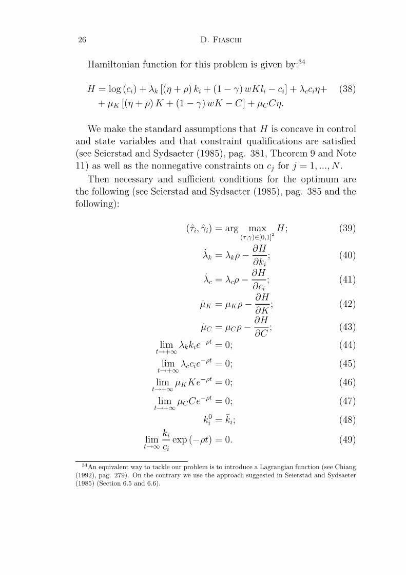
Hamiltonian function for this problem is given by:34

H = log (ci) + λk [(η + ρ) ki + (1 − γ)wKli − ci] + λcciη+ (38)

+ µK [(η + ρ)K + (1 − γ)wK − C] + µCCη.

We make the standard assumptions that H is concave in controland state variables and that constraint qualifications are satisfied

(see Seierstad and Sydsaeter (1985), pag. 381, Theorem 9 and Note11) as well as the nonnegative constraints on cj for j = 1, ..., N .

Then necessary and sufficient conditions for the optimum arethe following (see Seierstad and Sydsaeter (1985), pag. 385 and the

following):

(τi, γi) = arg max(τ,γ)∈[0,1]

2H; (39)

λk = λkρ−∂H

∂ki

; (40)

λc = λcρ−∂H

∂ci; (41)

µK = µKρ−∂H

∂K; (42)

µC = µCρ−∂H

∂C; (43)

limt→+∞

λkkie−ρt = 0; (44)

limt→+∞

λccie−ρt = 0; (45)

limt→+∞

µKKe−ρt = 0; (46)

limt→+∞

µCCe−ρt = 0; (47)

k0i = ki; (48)

limt→∞

ki

ciexp (−ρt) = 0. (49)

34An equivalent way to tackle our problem is to introduce a Lagrangian function (see Chiang(1992), pag. 279). On the contrary we use the approach suggested in Seierstad and Sydsaeter(1985) (Section 6.5 and 6.6).


From (39)-(43) we have:

∂H

∂τ

∣

∣

∣

∣

τ=τi,γ=γi

=

0 if 0 < τi < 1;≥ 0 if τi = 1;≤ 0 if τi = 0;

(50)

∂H

∂γ

∣

∣

∣

∣

τ=τi,γ=γi

=

0 if 0 < γi < 1;≥ 0 if γi = 1;

≤ 0 if γi = 0;

(51)

λk

λk

= ρ− (1 − τ) r; (52)

λc

λc

= 2ρ− 1

ciλc

+λk

λc

− (1 − τ) r; (53)

µK

µK

= ρ− rλk

µK

(1 − γ)

(

1 − α

α

)

li − r

[

(1 − τ) + (1 − γ)

(

1 − α

α

)]

;

(54)

µC

µC

= 2ρ+µK

µC

− (1 − τ) r, (55)

where σi = Kliki

and

∂H

∂τ= λk [ητki + (1 − γ)wτKli]+λcciητ+µKK [ητ + (1 − γ)wτ ]+µCCητ ;

∂H

∂γ= λk [ηγki + (1 − γ)wγKli − wKli]+λcciηγ+µKK [ηγ + (1 − γ)wγ − w]+µCCηγ.

AA. Candidate solution

A way to solve Problem P2 is to verify if a candidate solutionsatisfies necessary and sufficient conditions. In particular, we guess

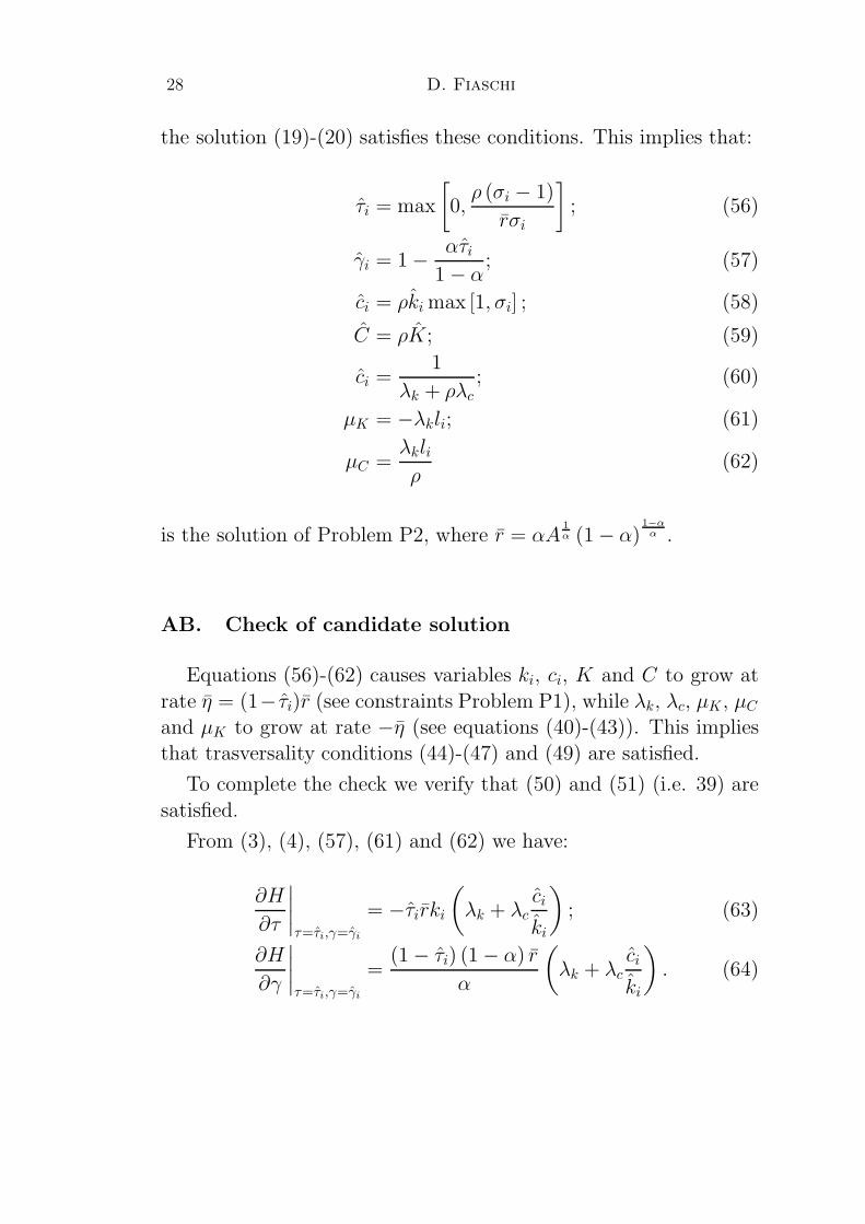
28 D. Fiaschi

the solution (19)-(20) satisfies these conditions. This implies that:

τi = max

[

0,ρ (σi − 1)

rσi

]

; (56)

γi = 1 − ατi

1 − α; (57)

ci = ρki max [1, σi] ; (58)

C = ρK; (59)

ci =1

λk + ρλc

; (60)

µK = −λkli; (61)

µC =λkli

ρ(62)

is the solution of Problem P2, where r = αA1α (1 − α)

1−αα .

AB. Check of candidate solution

Equations (56)-(62) causes variables ki, ci, K and C to grow at

rate η = (1− τi)r (see constraints Problem P1), while λk, λc, µK , µC

and µK to grow at rate −η (see equations (40)-(43)). This impliesthat trasversality conditions (44)-(47) and (49) are satisfied.

To complete the check we verify that (50) and (51) (i.e. 39) are

satisfied.

From (3), (4), (57), (61) and (62) we have:

∂H

∂τ

∣

∣

∣

∣

τ=τi,γ=γi

= −τirki

(

λk + λc

ci

ki

)

; (63)

∂H

∂γ

∣

∣

∣

∣

τ=τi,γ=γi

=(1 − τi) (1 − α) r

α

(

λk + λc

ci

ki

)

. (64)


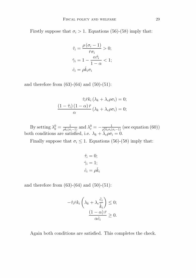
Firstly suppose that σi > 1. Equations (56)-(58) imply that:

τi =ρ (σi − 1)

rσi

> 0;

γi = 1 − ατi

1 − α< 1;

ci = ρkiσi

and therefore from (63)-(64) and (50)-(51):

τirki (λk + λcρσi) = 0;

(1 − τi) (1 − α) r

α(λk + λcρσi) = 0;

By setting λ0k = 1

ρki(σi−1)and λ0

c = − 1ρ2

i kiσi(σi−1)(see equation (60))

both conditions are satisfied, i.e. λk + λcρσi = 0.

Finally suppose that σi ≤ 1. Equations (56)-(58) imply that:

τi = 0;

γi = 1;

ci = ρki

and therefore from (63)-(64) and (50)-(51):

−τirki

(

λk + λc

ci

ki

)

≤ 0;

(1 − α) r

αci≥ 0.

Again both conditions are satisfied. This completes the check.

30 D. Fiaschi

B Derivation of equation (17)

The following are the first order conditions of problem (P1)

∂H

∂τ=

(1 − γ)wτσi

(1 − γ)wσi + ρ+ λki [(1 − τ) rτ − r] ; (65)

∂H

∂γ=σi [(1 − γ)wγ − w]

(1 − γ)wσi + ρ+ λki [(1 − τ) rγ] ; (66)

λ

λ= ρ− 1

λki

− [(1 − τ) r − ρ] , (67)

where rτ =∂r

∂τ, rγ =

∂r

∂γ, wτ =

∂w

∂τand wγ =

∂w

∂γ.

A solution to (67) is1

kiλ= ρ; (68)

Equations (68), (65) and (66) yield:

ρ

(1 − γ)wσi + ρ=r − (1 − τ) rτ(1 − γ)wτσi

; (69)

ρ

(1 − γ)wσi + ρ= − (1 − τ) rγ

σi [(1 − γ)wγ − w]. (70)

Substituting equation (69) in equation (70), given that w =(1−α)

αr, leads to

r − (1 − γ) rγ(1 − τ) rγ

=rτ (1 − γ)

r − (1 − τ) rτ,

from which

(1 − γ) (1 − α)2 − α2τ − α (1 − α) γ

− (1 − τ) (1 − α)2 =(1 − γ) (1 − α)

ατ + (1 − α) γ − (1 − α) (1 − τ),

and finally

τ =(1 − α) (1 − γ)

α, (71)

which represents equation (17). Finally, notice that (68) satisfiesthe transversality condition (16).


C Proof of Proposition 10

The proof consists in two steps: the first is to prove that if factor

endowments are even distributed, i.e. σi = 1 ∀i, then τE = 0,while the second step proves that if factor endowments are unevenly

distributed then τE > 0.

The first step is proved by verifying that 1) τE = 0 is a solution

of condition (34) if µσ = 1 and that 2) µσ = 1 ⇔ σi = 1 ∀i. The firstpoint follows directly from (35), while the second requires a lengthier

demonstration. First of all, note that the resource constraint impliesk1

lK+ ...+ kN

lK= 1

lor 1

σ1+ ...+ 1

σN= N35, which yields µσ =

∏Nj=1 σj.

Now let’s suppose for argument’ sake that µσ =∏N

j=1 σj = 1, but

that σq, σz 6= 1, where q, z ≤∈ {1, ..., N} and q 6= z. Since µσ =∏N

j=1 σj = 1 then σi+σz

2= 1, from which σq = 2 − σz and σqσz = 1;

but (2 − σz) σz = 1 implies (σz − 1)2 = 0 which is verified onlyfor σz = 1; this contradicts the assumption σz 6= 1. Therefore

µσ = 1 ⇔ σi = 1 ∀i.The second step is proved by induction. In particular, we verify

that an increase in inequality of endowment distribution due to a

reallocation of capital between two agents implies an increase in τE.In fact, starting from an even distribution of resources, it is intuitiveto conclude that any other feasible distribution can be generated by

a series of reallocations between two agents that increases inequal-ity; therefore, provided that an increase in inequality of endowment

distribution implies an increase in τE, all uneven distributions willbe characterized by a τE > 0.

Suppose that σq > σz, where q, z ∈ {1, ..., N} and to redistributesome quantity of capital from agent q to agent z; this causes an

increase in σq and a fall in σz, that is an increase in inequality.Moreover let k = kq + kz be the total amount of capital of two

agents, from which 1σq

+ 1σz

= 1σ, where σ = Kl

kis a constant. It

easily follows that σz =σσq

σq−σand dσz

dσq= − σ2

(σq−σ)2 .

35Indeed if L = 1 and li = l ∀i, then l = 1N

.

32 D. Fiaschi

Now calculate the total differential of (34), that is:

dτE

(

∑N

j=1

rσ2j

(τE rσj + ρ)2

)

=∑N

j=1

[

ρ

(τE rσj + ρ)2

]

dσj

and, provided that 1σq

+ 1σz

= 1σ

and dσi = 0 ∀i, i 6= q, z, the aboveequation becomes

dτE

(

∑N

j=1

rσ2j

(τE rσj + ρ)2

)

=

= ρ

1

(τE rσq + ρ)2 − σ2

(

τE r(

σσq

σq−σ

)

+ ρ)2

(σq − σ)2

dσq,

hence:

dτE

(

∑N

j=1

rσ2j

(τE rσj + ρ)2

)

= ρ

[

(

2τE rσq + ρ)

(σq − 2σ)σqρr

(τE rσq + ρ)2 (τE rσσq + ρ (σq − σ))2

]

dσq.

It follows that:

dτE > 0 ⇔ σq − 2σ > 0,

that isdτE > 0 ⇔ σq > σz.

This completes the proof.

D Leisure in utility function

The aim of this Appendix is to show how the fiscal policy whichmaximizes the growth rate changes if labor has an elastic supply.

For simplicity the log-linear utility case will be analyzed, that is:

Vi = (1 − φ) log ci + φ log pi,

where pi is leisure and φ ∈ [0, 1] measures the elasticity of substi-

tution between leisure and working time. By normalizing to1

Nthe


total amount of time disposable per period to each agent it follows

that:

pi =1

N− li.

As in the case of inelastic labor supply, wage and interest rate

are defined by:

r = αA1α [ατ + (1 − α) γ]

1−αα L

1−αα = r (τ, γ) ; (72)

w = (1 − α)A1α [ατ + (1 − α) γ]

1−αα L

1−2αα K = w (τ, γ)K, (73)

where L =∑N

i=1 li.Agent i solves

max{ci,li}∞t=0

Ui =

∞∫

0

e−ρt

[

(1 − φ) log ci + φ log

(

1

N− li

)]

dt (74)

ki = (1 − τ)r(τ, γ)ki + (1 − γ)w(τ, γ)Kli − ci. (75)

The first order conditions (necessary and sufficient for the opti-

mum) are

1 − φ

ci= λ; (76)

φ

1

N− li

= λ (1 − γ)w(τ, γ)K; (77)

λ = λ [ρ− (1 − τ) r(τ, γ)] ; (78)

limt→∞

e−ρtλki = 0. (79)

It is possible to show (see (76), (78) and (79)) that the steadystate growth rate is

η(τ, γ) =ci

ci=ki

ki

= (1 − τ) r(τ, γ)− ρ (80)

and therefore from (75) the level of consumption is:

ci = (1 − γ)w(τ, γ)liK + ρki.

34 D. Fiaschi

The latter can be used to calculate the optimal level of working

time:

li =1 − φ

N− φρki

(1 − γ)w(τ, γ)K.

By aggregating it yields the aggregate supply curve of labor

L = (1 − φ) − φρ

(1 − γ)w(τ, γ). (81)

Note that w(τ, γ) is a nonlinear function of L (see (73)) and this,in general, does not allow an analytical solution. Since the intention

of this Appendix is only to provide an example of the effects of anelastic supply of labor, for the sake of simplicity in order to obtain

an analytical solution set α = 12.

The steady state growth rate will be given by ( see (72), (80) and

(81))

η(τ, γ) =1

2(1 − τ)

[

(

γ+τ2

)

(1 − φ) − 2φρ(1−γ)

]

− ρ.

The derivative of η with respect to γ is equal to

∂η(τ, γ)

∂γ=

1

2(1 − τ)

[

1 − φ

2− 2φρ

(1 − γ)2

]

,

from which:

γ∗ = min

[

0, 1 − 2

√

φρ

(1 − φ)

]

.

Thus, if φ > 0 then γ∗ < 1 and∂γ∗

∂φ≤ 0, strictly if φ < 1

1+4ρ

(see Section II.A.); it is worth noting that this result contrasts withLucas (1990). However many empirical works have found φ very

low, so that setting φ = 0 does not seem a very strong assumption.The derivative of η with respect to τ is equal to

∂η(τ, γ)

∂τ=

1

2

[

2φρ

(1 − γ)2 +(1 − φ) (1 − γ)

2− τ (1 − φ)

]

,

from which:

τ ∗ = min

[

2φρ√

φρ (1 − φ), 1

]

.


Therefore, τ ∗ = 0 iff φ = 0 (the case of inelastic labor supply) and∂τ ∗

∂φ≥ 0, strictly if φ < 1

1+4ρ; finally, if φ > 1

1+4ρthen (τ ∗, γ∗) = (1, 0)

and the steady state growth rate will be negative.

E CES utility function

This Appendix extends the analysis to the case where the utilityis:

(ci)1−µ − 1

1 − µ,

that is, the elasticity of substitution of consumption is constant and

equal to 1µ. We stress that a CES utility function is a necessary

condition to have a steady state.

The i-th agent solves

max{ci}∞t=0

Ui =

∞∫

0

e−ρt (ci)1−µ − 1

1 − µdt (P1.A)

s.t. ki = ki [(1 − τ)r(τ, γ) + (1 − γ)w(τ, γ)σi] − ci.

Given the time paths both of the taxes and of the capital aggregate

stock, the solution of problem (P1.A) yields the following optimalconsumption path:

ci

ci=

(1 − τ)r(τ, γ)− ρ

µ. (82)

It is possible to demonstrate that (82) is also the growth rate of Kand ki, such that

ci

ci=ki

ki

=K

K=

(1 − τ)r(τ, γ)− ρ

µ= η (τ, γ) . (83)

Therefore η (τ, γ) is the steady state growth rate; finally, theinstantaneous level of consumption along the optimal path is givenby:

ci =[(µ− 1) (1 − τ) r(τ, γ) + µ (1 − γ)w(τ, γ)σi + ρ] ki

µ.

36 D. Fiaschi

The optimal fiscal policy for the i-th agent solves:

max{τ,γ}∞t=0

Ui =

∞∫

0

e−ρt (ci)1−µ − 1

1 − µdt

s.t.

ci =[(µ− 1) (1 − τ) r(τ, γ) + µ (1 − γ)w(τ, γ)σi + ρ] ki

µki

ki

=K

K= η (τ, γ) .

(P2.B)

Assume thatρ

r+ (µ− 1) > 0 in order to have for every feasible

τ a definite integral in (P2.B). The current value Hamiltonian of

problem (P2.B) is given by

H ={[(µ− 1) (1 − τ) r(τ, γ) + µ (1 − γ)w(τ, γ)σi + ρ] ki}1−µ

µ1−µ (1 − µ)+

(84)

+ λki

[

(1 − τ) r (τ, γ)− ρ

µ

]

− 1

µ1−µ (1 − µ).

The following are the necessary and sufficient conditions for the

optimum:

∂H

∂τ= 0, (85)

∂H

∂γ= 0, (86)

λ = ρλ− ∂H

∂ki

and (87)

limt→∞

e−ρtλki = 0. (88)

From equations (85), (86) and (87), it follows that:36

τ =(1 − α) (1 − γ)

α. (89)

36The calculations are available on request.


Hence, substituting (89) in (85):

τi = max

0,

(σi − 1)[ρ

r+ (µ− 1)

]

µ (σi − 1) + 1

, (90)

where r = αA1α (1 − α)

1−αα is the value of r when (89) holds.

On the assumption that tax rates are constant, solving the inte-gral in (P2.B) yields the following expression for individual utility:

Ui (σi, τ, γ) =[(µ− 1) (1 − τ) r (τ, γ) + µ (1 − γ)w (τ, γ)σi + ρ]1−µ

µ1−µ (1 − µ) (ki0)

µ−1[ρ− (1 − µ) η (τ, γ)]

+

(91)

− 1

ρ (1 − µ).

It is analytically convenient to focus attention only on fiscal poli-

cies which can be a Pareto optimum; substituting (89) in (91) andby using the relationship w (τ, γ) =

(

1−αα

)

r (τ, γ), it follows that:

U (σi, τ) =µµ(

ki0

)1−µ [

µτσi − (1 − µ) (1 − τ) + ρr

]1−µ

(1 − µ) rµ[

ρr− (1 − µ) (1 − τ)

] − 1

ρ (1 − µ).

Notice that U is concave with respect to τ if:37

µσi − µ+ 1 > 0;

since this condition has to hold for every i, assume that

µ <1

1 − σ, (92)

where σ = min {σi}Ni=1 ≤ 1.

37In fact:

∂2U

∂τ2= r (Kli)

1−µ

[

1 − r−µ−1σµ−1i µµ+1 (µσi − µ + 1)

(

µτσi + (1 − τ) (µ − 1) + ρr

)µ (− (1 − τ) (µ − 1) − ρr

)2

]

,

from which a necessary condition to have ∂2U∂τ2 > 0 is (µσi − µ + 1) > 0.

38 D. Fiaschi

EA. Maximum growth

The following Propositions state the fiscal policies that maximizethe growth rate and that of politico-economic equilibrium:

Proposition 11 The fiscal policy that maximizes the growth rateη (τ, γ) is given by (τ ∗, γ∗) = (0, 1).

Proof. Consider the derivative of equation (11) with respect to τ

and γ. Since∂η (τ, γ)

∂τ> 0 ⇔ τ < (1 − α) (1 − γ) and

∂η (τ, γ)

∂γ>

0 ∀ (τ, γ), then the fiscal policy which maximizes growth is givenby (τ ∗, γ∗) = (0, 1).

In the following assume that every agent has the same laborendowment, such that a difference in σ reflects different capital en-

dowments, that is:

li = l =1

N∀i ∈ {1, ..., N} . (93)

Moreover, to avoid trivial results assume, unless otherwise spec-ified, that σ is unevenly distributed, that is:

∃i, j ∈ {1, ..., N} with i 6= j such that σi 6= σj.

EB. Normative analysis

As stated above we focus our attention only on fiscal policiessatisfying relationship (89). Substituting for γ in (91) yields the set

of all individual utilities associated to τ :[

U (σ1, τ) , ... , U (σN , τ)]

,

whose elements are ranked in increasing order, i.e. U (σ1, τ) ≤U (σ2, τ) ≤ ... ≤ U (σN , τ).

Assume that the welfare function is additive-separable, that is:

W =

N∑

j=1

φ(

U (σj, τ))

; (94)


Let τW be the tax rate on capital income which maximizes thewelfare function, that is

τW = arg maxτ

[

N∑

j=1

φ(

U (σj, τ))

]

. (95)

Let the (generalized) Lorenz curve be:

GLτ (p) =

S∑

j=1

U (σi, τ)

N=

=1

N

S∑

j=1

µµ(

ki0

)1−µ [

µτσi − (1 − µ) (1 − τ) + ρr

]1−µ

(1 − µ) rµ[

ρr− (1 − µ) (1 − τ)

] − S

Nρ (1 − µ)

for S = 1, ..., N and where p = SN

and r = αA1α (1 − α)

1−αα .

The first derivative ofGL (p, τ) with respect to τ shows how fiscalpolicy affects the Lorenz curve:

∂GL (p, τ)

∂τ=

S∑

j=1

(Kl)1−µµµ+1σ

µ−1j

[

(σj − 1)(

ρr− 1 + µ (1 − τ)

)

− τ]

Nrµ[

ρr+ µτσj − (1 − µ) (1 − τ)

]µ [

(1 − τ) (1 − µ) − ρr

] .

(96)

The following Proposition states the optimal fiscal policy for a

Rawlsian social planner:

Proposition 12 Let(

τR, γR)

be the optimal fiscal policy when thesocial planner has Rawlsian preferences. Then τR maximizes GL

(

1N, τ)

,that is:

τR = max

[

0,(σ1−1)

[

ρr+(µ−1)

]

µ(σ1−1)+1

]

(97)

and

γR = min

[

1, 1 −α(σm−1)

[

ρr+(µ−1)

]

(1−α)[µ(σm−1)+1]

]

. (98)

Proof. To prove (97) it is sufficient to note that U (σ1, τ) ≤U (σ2, τ) ≤ ... ≤ U (σN , τ), while γR is derived from (89).

40 D. Fiaschi

The following Proposition states the optimal fiscal policy when

welfare is the simple sum of individual utilities, that is efficiency isthe only goal of the social planner:

Proposition 13 Let(

τE, γE)

be the optimal fiscal policy when wel-

fare is the simple sum of individual utilities. Then τE maximizesGLτ (1), that is:

∂GLτ (1)

∂τ

∣

∣

∣

∣

τ=τE

= 0 (99)

and

γE = 1 −(

α

1 − α

)

τE. (100)

Proof. The proof of (99) is given by the same definition of the

generalized Lorenz curve, while γE is derived from (89).Since τE solves the condition (99), i.e.

∂GLτ (1)

∂τ

∣

∣

∣

∣

τ=τE

= 0 (101)

⇔N∑

j=1

σµ−1j

[

(σj − 1)(

ρr− 1 + µ

(

1 − τE))

− τE]

[

ρr+ µτEσj − (1 − µ) (1 − τE)

]µ = 0,

it follows that τR ≥ τE. Indeed, note that:38

σµ−11

[

(σ1 − 1)(

ρr− 1 + µ (1 − τ)

)

− τ]

[

ρr+ µτσ1 − (1 − µ) (1 − τ)

]µ ≥

σµ−1j

[

(σj − 1)(

ρr− 1 + µ (1 − τ)

)

− τ]

[

ρr

+ µτσj − (1 − µ) (1 − τ)]µ

∀j = 2, ..., N and ∀τ ∈ [0, 1], from which

N∑

j=1

σµ−1j

[

(σj − 1)(

ρr− 1 + µ

(

1 − τR))

− τR]

[

ρr

+ µτRσj − (1 − µ) (1 − τR)]µ ≤ 0,

38Since (µσi − µ + 1) > 0 ∀i (see (92)), then

∂2U

∂τ∂σj

=σ

µ−2j (Kl)

1−µr−µµµ+1 (µσj − µ + 1)

(

µτσj + (1 − τ) (µ − 1) + ρr

)1+µ> 0.


that yields τR ≥ τE. Heuristically the set of all possible τW be-longs to the interval

[

τE, τR]

, and the higher the social planner’s

inequality aversion, the closer is τW to τR.To examine this point in greater depth, note that since σ1 ≥ σ1 ≥

... ≥ σN then:

S∑

j=1

σµ−1j [(σj−1)( ρ

r−1+µ(1−τ))−τ]

[ρr+µτσj−(1−µ)(1−τ)]

µ

S≥

S+1∑

j=1

σµ−1j [(σj−1)(ρ

r−1+µ(1−τ))−τ]

[ρr+µτσj−(1−µ)(1−τ)]

µ

S + 1(102)

for S ∈ [1, N − 1] and ∀τ ∈ [0, 1].

Given that τE has to satisfy the following equality:

N∑

j=1

σµ−1j

[

(σj − 1)(

ρr− 1 + µ

(

1 − τE))

− τE]

[

ρr+ µτEσj − (1 − µ) (1 − τE)

]µ = 0,

it follows that:

∂GLτ (p)

∂τ

∣

∣

∣

∣

τ=τE

=S∑

j=1

σµ−1j

[

(σj − 1)(

ρr− 1 + µ

(

1 − τE))

− τE]

[

ρr

+ µτEσj − (1 − µ) (1 − τE)]µ ≥ 0

for S = 1, ..., N − 1.

This means that the Lorenz curve corresponding to τE is every-where increasing in τE, except for p = 1; in other words, an increase

in τE causes a decrease in inequality, but also a decrease in averageutility. Let τS be the level of tax rate that if increased would leaveGLτ (p) unchanged, that is:

∂GLτ (p)

∂τ

∣

∣

∣

∣

τ=τS

= 0.

From (102) it follows that vector {τS}NS=1 is ranked in decreas-

ing order, i.e. τS ≥ τS+1, such that τ1 = τR and τN = τE (see

Propositions 12 and 13).

Proposition 14 Let W =N∑

j=1

φ(

U (σj, τ))

be the social welfare

function, where φ′ ≥ 0, φ′′ ≤ 0, U (σi, τ) the intertemporal utility

42 D. Fiaschi

of agent i and U (σi, τ) ≤ U (σi+1, τ) for i = 1, ..., N − 1. Then the

tax rate on capital income maximizing welfare function τW has to

belong to the interval[

τE, τR]

, where τR = max

[

0,(σ1−1)

[

ρr+(µ−1)

]

µ(σ1−1)+1

]

and τE implicitly solvesN∑

j=1

σµ−1j [(σj−1)(ρ

r−1+µ(1−τE))−τE]

[ρr+µτEσj−(1−µ)(1−τE)]

µ = 0.

Moreover, according to Definitions 4 and 5, τE is the most efficientfiscal policy, while all fiscal policies belonging to the interval

(

τE, τR)

present an efficiency-equity trade-off.

Proof. From (102) it follows that τS ≥ τS+1, and since τE maxi-mizes the simple sum of individual utility, then in every economy

where τ < τE average individual utility is lower and inequality ishigher than in the economy where τ = τE; this means that any

τ < τE cannot maximize social welfare. Moreover, in every econ-omy where τ > τR average individual utility is lower and the poorestagent is worse off than in the economy where τ = τR; therefore the

tax rate on capital income maximizing welfare function τW has tobelong to the range

[

τE, τR]

. This proves the first statement. The

proof of the second statement directly follows from Definitions 4and 5 and equation (96).

EB.i. Efficient fiscal policy

According to Definition 4 the most efficient fiscal policy maxi-mizes the simple sum of individual utilities, that is:

(

τE, τE)

= arg maxτ,γ

W =

=1

N

S∑

j=1

µµ(

ki0

)1−µ [

µτσi − (1 − µ) (1 − τ) + ρr

]1−µ

(1 − µ) rµ[

ρr− (1 − µ) (1 − τ)

] − S

Nρ (1 − µ)

By the first order conditions it follows that:

τ =(1 − α) (1 − γ)

α

and


N∑

j=1

σµ−1j

[

(σj − 1)(

ρr− 1 + µ

(

1 − τE))

− τE]

[

ρr

+ µτEσj − (1 − µ) (1 − τE)]µ = 0. (103)

Setting τE = 0 in (34) yields a sufficient condition to obtainτE = 0, that is

N∑

j=1

σµ−1j (σj − 1) = 0, (104)

that is σi = 1 ∀i (or µσ = 1).39

The following Proposition characterizes the most efficient fiscal

policy:

Proposition 15 The most efficient fiscal policy (or the optimal fis-cal policy when the social planner is indifferent to inequality) in-

volves a positive tax rate on capital income, but the case of evendistribution of individual endowments (i.e. the representative agent

economy); that is:

τE =

{

0 if σi = 1 ∀iψ > 0 if ∃i such that σi 6= 1

Proof. This proof follows closely that of Appendix C. The proofconsists of two steps: the first is to prove that if factor endowments

are evenly distributed, i.e. σi = 1 ∀i, then τE = 0, while the secondthat, if factor endowments are unevenly distributed, then τE > 0.The first step is proved by verifying that 1) τE = 0 is a solution of

condition (103) if µσ = 1 and that 2) µσ = 1 ⇔ σi = 1 ∀i. Thefirst point follows directly from (104), while for the second refer to

Appendix C. The second step is proved by verifying that an increasein inequality of endowments’ distribution due to a reallocation of

capital between two agents implies an increase in τE. Suppose thatσq > σz, where q, z ∈ [1, N ] and to redistribute some quantity ofcapital from agent q to agent z; this causes an increase in σq and a

39See Appendix C.

44 D. Fiaschi

fall in σz, that is an increase in inequality. Moreover, let k = kq +kz

be the total amount of capital of two agents, from which 1σq

+ 1σz

= 1σ,

where σ = Klk

is a constant. It easily follows that σz =σσq

σq−σand

dσz

dσq= − σ2

(σq−σ)2. Given the total differential of (94), that is:

dτE

(

∑N

j=1

∂2W

∂τ 2

)

= −∑N

j=1

∂2W

∂τ∂σj

dσj,

where ∂2W∂τ2 ≤ 0,40 provided that 1

σq+ 1

σz= 1

σ, dσq > 0, dσz = − σ2dσq

(σq−σ)2

and dσi = 0 ∀i, i 6= q, z, the above equation becomes

dτE

(

−∑N

j=1

∂2W

∂τ 2

)

=µµ+1 (Kl)1−µ

r

σ2q

{

σµq (µσq − µ+ 1)

[r (1 − τ) (µ− 1) + ρ+ µτ rσq](1+µ)

+

− σµz (µσz − µ+ 1)

[r (1 − τ) (µ− 1) + ρ+ µτ rσz](1+µ)

}

dσq,

hence:

dτE > 0 ⇔σµ

q (µσq − µ+ 1)

[r (1 − τ) (µ− 1) + ρ+ µτ rσq](1+µ)

+

− σµz (µσz − µ+ 1)

[r (1 − τ) (µ− 1) + ρ+ µτ rσz](1+µ)

> 0.

The last inequality holds if:41

σµq (µσq − µ+ 1) [r (1 − τ) (µ− 1) + ρ+ µτ rσz]

(1+µ)

σµz (µσz − µ+ 1) [r (1 − τ) (µ− 1) + ρ+ µτ rσq]

(1+µ)> 1,

that is:(

σq [r (1 − τ) (µ− 1) + ρ+ µτ rσz]

σz [r (1 − τ) (µ− 1) + ρ+ µτ rσq]

)µ

∗

∗(

(µσq − µ+ 1) [r (1 − τ) (µ− 1) + ρ+ µτ rσz]

(µσz − µ+ 1) [r (1 − τ) (µ− 1) + ρ+ µτ rσq]

)

> 1.

It is easy to check that both members are greater than 1, such that

dτE > 0.40This is the second order condition to have a maximum.41For condition (92) both µσq − µ + 1 and µσz − µ + 1 are nonegative.


6

-.............................................

1 p

GLτ (p)

...........................p

6

?

GLτA

(p)

GLτB

(p)

Figure 1: efficiency-equity trade-off

6

-.............................................

1 p

GLτ (p)

...........................S

N

6

?GLτS(p)

Figure 2: effect of an increase in τ

46 D. Fiaschi

6

........... -

1

σ1

σ2

Resource constraint

.......... ..1

1

7Iso-tax curve τE = 0

*Iso-tax curve τE > 0

Figure 3: two agent economy


References

Alesina, A. and Rodrik, D.: 1994, Distributive politics and economic

growth, Quarterly Journal of Economics 109(2), 493–490.

Barro, R. and Sala-I-Martin, X.: 1999, Economic Growth, MITPress, London, England.

Benhabib, J., Rustichini, A. and Velasco, A.: 2001, Public spend-

ing and optimal taxes without commitment, Review of EconomicDesign 6, 371–396.

Bertola, G.: 1993, Factor shares and savings in endogenous growth,

American Economic Review 81, 1184–1198.

Chamley, C. P.: 1986, Optimal taxation of capital income in generalequilibrium with infinite lives, Econometrica 54(3), 607–622.

Chiang, A.: 1992, Elements of Dynamics Optimization, McGrawHill, New York.

Correia, I. H.: 1999, On the efficiency and equity trade-off, Journal

of Monetary Economics 44, 581–603.

Dardanoni, V. and Lambert, P.: 1988, Welfare ranking of incomedistribution: A role for the variance and some insights for tax

reforms, Social Choice and Welfare 5(1), 1–17.

Jones, L., Manuelli, R. and Rossi, P.: 1997, On the optimal taxationof capital income, Journal of Economic Theory 73, 93–117.

Judd, K.: 1985, Redistributive taxation in a simple perfect foresightmodel, Journal of Public Economics 28, 59–83.

Judd, K. L.: 1999, Optimal taxation and spending in general com-

petitive growth models, Journal of Public Economics 71, 1–26.

Karcher, T., Moyes, P. and Trannoy, A.: 1995, The stochastic dom-inance ordering of income distributions over time: The disconted

48 D. Fiaschi

sum of the expected utilities of incomes, in W. B. et Al. (ed.), So-

cial Choice, Welfare, and Ethics: Proceedings of the Eighth Inter-national Symposium in Economic Theory and Econometrics, Cam-

bridge University Press, New York and Melbourne, pp. 375–408.

Lansing, K.: 1999, Optimal redistributive capital taxation in a neo-classical growth model, Journal of Public Economics 73, 423–453.

Lucas, R. E.: 1990, Supply-side economics: an analytical review,Oxford Economic Papers 42, 293–316.

Seierstad, A. and Sydsaeter, K.: 1985, Optimal Control Theory withEconomic Applications, North-Holland, Amsterdam.

Shorrocks, A. F. and Foster, J. E.: 1987, Transfer sensitive inequal-ity measures, Review of Economic Studies 3(179), 485–497.

Stiglitz, J.: 1987, Pareto efficient and optimal taxatation and thenew welfare economics, in A. Auerbach and M. Feldstein (eds),Handbook of Public Economics Vol. II, Vol. II, North-Holland.

Discussion Papers – Collana del Dipartimento di Scienze Economiche – Università di Pisa

1. Luca Spataro, Social Security And Retirement Decisions In Italy, (luglio 2003) 2. Andrea Mario Lavezzi, Complex Dynamics in a Simple Model of Economic

Specialization, (luglio2003) 3. Nicola Meccheri, Performance-related-pay nel pubblico impiego: un'analisi

economica, (luglio 2003) 4. Paolo Mariti, The BC and AC Economics of the Firm, (luglio 2003) 5. Pompeo Della Posta, Vecchie e nuove teorie delle aree monetarie ottimali,

(luglio 2003) 6. Giuseppe Conti, Institutions locales et banques dans la formation et le

développement des districts industriels en Italie, (luglio 2003) 7. F. Bulckaen - A. Pench - M. Stampini, Evaluating Tax Reforms through

Revenue Potentialities: the performance of a utility-independent indicator,

(settembre 2003) 8. Luciano Fanti - Piero Manfredi, The Solow’s model with endogenous

population: a neoclassical growth cycle model (settembre 2003) 9. Piero Manfredi - Luciano Fanti, Cycles in dynamic economic modelling

(settembre 2003) 10. o Alfredo Minerva, Location and Horizontal Differentiation under Gaetan

Duopoly with Marshallian Externalities (settembre 2003) 11. ano Fanti - Piero Manfredi, Progressive Income Taxation and Economic Luci

Cycles: a Multiplier-Accelerator Model (settembre 2003) 12. Della Posta, Optimal Monetary Instruments and Policy Games Pompeo

Reconsidered (settembre 2003) 13. vide Fiaschi - Pier Mario Pacini, Growth and coalition formation (settembre Da

2003) 14. vide Fiaschi - Andre Mario Lavezzi, Nonlinear economic growth; some Da

theory and cross-country evidence (settembre 2003) 15. ano Fanti , Fiscal policy and tax collection lags: stability, cycles and chaos Luci

(settembre 2003) 16. olfo Signorino- Davide Fiaschi, Come scrivere un saggio scientifico:regole Rod

formali e consigli pratici (settembre 2003) 17. ano Fanti, The growth cycle and labour contract lenght (settembre 2003)Luci 18. nd Welfare in an Endogenous Growth Model Davide Fiaschi , Fiscal Policy a

with Heterogeneous Endowments (ottobre 2003)

19. ano Fanti, Notes on Keynesian models of recession and depression, Luci

(ottobre 2003) 20. no Fanti, Technological Diffusion and Cyclical Growth, (ottobre 2003) Lucia 21. ano Fanti - Piero Manfredi, Neo-classical labour market dynamics, chaos Luci

and the Phillips Curve, (ottobre 2003) 22.

Redazione: Giuseppe Conti

Luciano Fanti – coordinatore Davide Fiaschi

Paolo Scapparone

Email della redazione: [email protected]

mailto:[email protected]

fiscal policy and welfare in an endogenous growth model with … · 2018-05-30 · growth model...

Documents