Modeling & Managing Sovereign & Systemic Risk

Fiscal Solvency & Macroeconomic Uncertainty in Emerging Markets:

The Tale of the Tormented Insurer

Enrique G. Mendoza P. Marcelo OviedoIMF, Univ. of Maryland Iowa State University& NBER

The fiscal problem of emerging economies

1. High, growing public debt (mostly nsc instruments)Driven by financial instability, not standard primary deficits

2. Low and volatile public revenue ratios Dependent on non-tax components (commodity exports) Average debt ratios fall as revenue variability rises

3. Fiscal policies display abnormal cyclical behaviorGDP correlations of primary balance (gov. expenditures) close to zero or slightly negative (positive)Downward rigidities in cutting outlays, cuts in “bad times”Excess variability of public relative to private expenditures

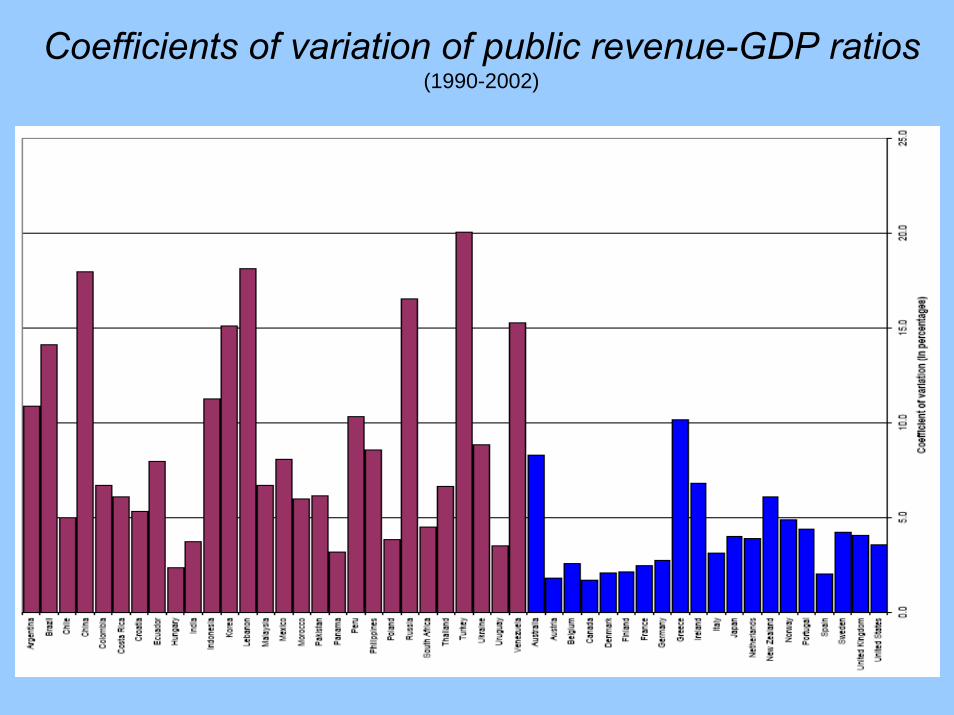
Coefficients of variation of public revenue-GDP ratios (1990-2002)

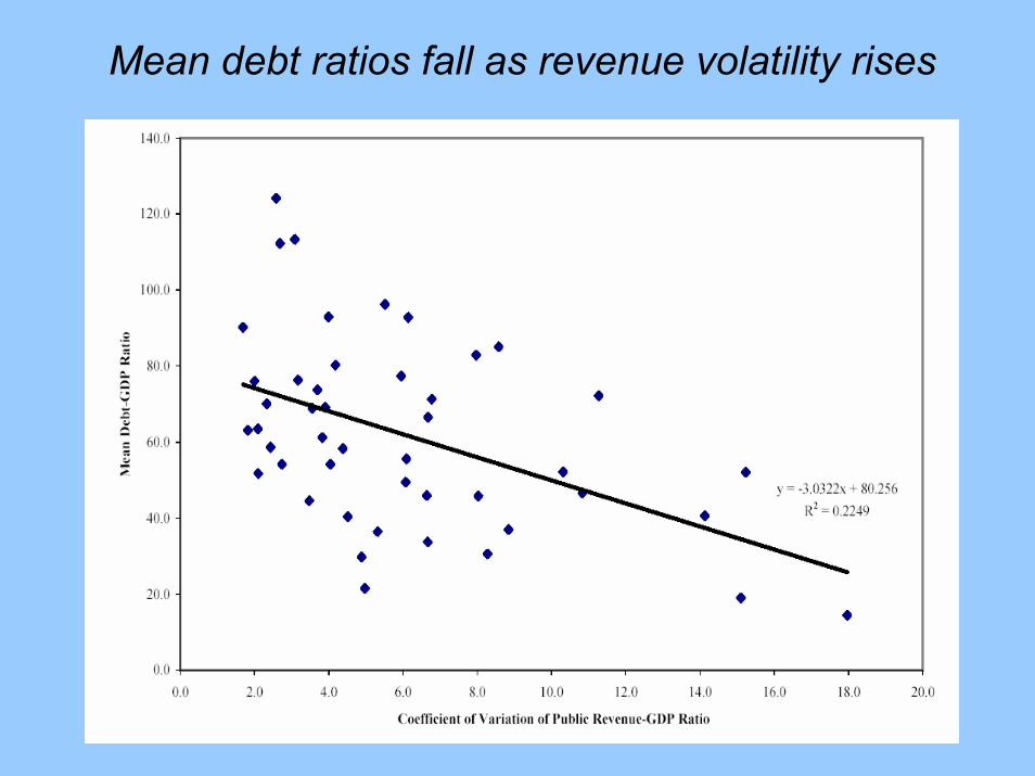
Mean debt ratios fall as revenue volatility rises

Excess variability of government purchases relative to private expenditures

The EMs fiscal dilemma: A problem of social insurance

Institutions & policies split domestic income between private and public sectors

1st best: Pool incomes, equate mg. ut. of expenditures– Needs state-contingent, non-distorting taxes, transfers or debt

2nd best: Choose optimal debt & expenditures policies given limited debt instruments, low/volatile revenues, fiscal rigidities– Sustainable debt has a self insurance feature

Debt sustainability analysis requires:– EM features: suboptimal taxes, credit frictions, macro volatility,

policy rigidities– Forward looking, structural treatment (Lucas critique argument)

Solving the 2nd best problem:The tormented insurer framework

Gov. aims to smooth its outlays relative to the volatility of revenues but using only non-state-contingent debt

Sustainable debt features a Natural Debt Limit– NDL = annuity value of primary balance at fiscal crisis– Fiscal crisis: long sequence of low revenues, outlays cut to

lowest “tolerable” levels– NDL is also a credible commitment to be able to repay, but is

NOT generally the same as sustainable debt, which is set by budget constraint

Structural DSGE tool for public/external debt analysis: – Calibrated to country-specific features– Models explicitly gov. behavior and GE of the economy

Basic model: random revenue, ad-hoc outlays

Gov. budget constraint:

Markov process of revenues: t ε [tmin,tmax], π

Fiscal crisis: “almost surely”,

Gov. keeps as long as it can access debt market

NDL:

– “classic” sustainability ratio exceeds NDL since it uses E[t-g]

Sustainable debt: 11 min ,g g

t t tb g t b Rγ φ−+ ⎡ ⎤= − +⎣ ⎦

mintg g=

m in m in

1gt

t gbR

φγ+

−≤ =

−

mintt t=

tg g=

1 ( )g gt t t t tb b R t gγ + = − −

Lessons from the basic model

Higher revenue volatility tightens NDL (↓tmin as ↑sd(t) )

Commitments to repay & cut outlays at fiscal crisis support each other– Given t process, countries with lower can borrow more,

and are less likely to face fiscal crisis

Insurance argument in favor of indirect taxation

Degenerate long-run debt distribution: debt converges to NDL or vanishes depending on initial conditions

– “Time to fiscal crisis:”

ming

m in

m in

R g gg t

T

γ⎛ ⎞ −

=⎜ ⎟ −⎝ ⎠

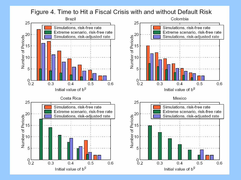
Application of the basic model (cont’d)Brazil Colombia Costa Rica Mexico

Public debt 1990-2002 1990-2002 1990-2002 1990-2002average 40.68 33.71 49.46 45.92maximum 56.00 50.20 53.08 54.90year of maximum 2002 2002 1996 1998

Implied fiscal adjustment to support maximum debt as NDL in no. of std. deviations 2.55 2.30 1.16 2.02 in % of GDP 6.73 3.99 2.15 1.54

Benchmark Natural Debt Limits(1961-2000 per-capita growth rates, 5% real interest rate)Growth rate 2.55 1.86 1.83 2.20Natural debt limit 56.09 50.49 53.31 54.92

Growth Slowdown Scenario(1981-2000 per-capita growth rates)Growth rate 0.48 1.05 1.25 0.83Natural debt limit 30.34 40.10 45.10 36.96

High Real Interest Rate Scenario(8% real interest rate)Growth rate 2.55 1.86 1.83 2.20Natural debt limit 25.19 25.81 27.39 26.53

The DSGE model

Public debt and expenditure policies are endogenous– Government’s behavior as insurer is endogenous– Gov. maximizes CRRA payoff (provides incentive to smooth and

yields NDL as feature of optimal plans)– Non-state-contingent debt

Private sector chooses NFA, public debt & consumption

Strategic interaction between public & private sectors– Markov perfect equilibrium– Two forms of market incompleteness: vis-à-vis rest of the world

and between domestic private and public sectors– Public and private precautionary savings motives

Stochastic output & taxes induce revenue volatility

Markov-perfect equilibrium

Government:

Private sector:

Market-clearing and Markov eq. conditions:

[ ]

11

,( , , ) max ( , , )

1

. . ,

( , , ), | , ( , ),

g

g I g I

b g

g g

I g I g g

gV b b e E V b b e

s t g z b y b

b b b e e e e y b

σσβγ

σ

τ

τ φ

′

−−⎧ ⎫⎪ ⎪⎡ ⎤⎪ ⎪′ ′ ′= +⎨ ⎬⎢ ⎥⎣ ⎦⎪ ⎪−⎪ ⎪⎩ ⎭

′+ + ℜ = +

′ ′′Π ≡ ≤

[ ]

11( , , ) max ( , , )

1

. . (1 ) ( ) ,

( , , ), | ,

I

g I g I

b

g I g I

g g I I I

cW b b e E W b b e

s t c x y z b b b b

b b b e e e b

σσβγ

σ

τ

φ

′

−−⎧ ⎫⎪ ⎪⎡ ⎤⎪ ⎪′ ′ ′= +⎨ ⎬⎢ ⎥⎣ ⎦⎪ ⎪−⎪ ⎪⎩ ⎭′ ′+ = − + − − + + ℜ

′ ′′Π ≥

( ) ( ), ( ) ( ),g g I I I Ib b b b c g x y b b′ ′ ′ ′ ′⋅ = ⋅ ⋅ = ⋅ + + = − + ℜ

Application to MexicoMexico’s GDP and “implied tax” processes:

Main results:1. 53% mean debt ratio, but fluctuations are highly persistent2. Acylical gov. purchases and primary balance3. Average debt ratios fall as volatility increases4. 1.6 to 3.5% welfare costs due domestic incompleteness

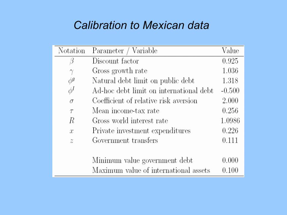
Calibration to Mexican data

Moments of the stochastic long-run equilibrium

Revenue variability and average public debt ratios

Impulse response functions of c/g ratio

Stochastic simulations of debt-GDP ratio(starting from initial condition of 63.4%)

Conclusions

Method to assess fiscal solvency in emerging economies with “tormented insurer” featuresPolicy implication: VATs may be useful for producing higher, stable revenues & enhance flexibility of outlays

Basic model:– Debt exceeds NDL in two out of four countries– In GS, HRIR scenarios debt is too high in all four countries– Short time to fiscal crisis for repeated negative shocks

DSGE model (applied to Mexico):– Current debt ratio of 45% and an average debt ratio of 53% are

consistent with fiscal solvency– Accounts for acyclical expenditures and primary balance– Accounts for link between lower debt and higher volatility– Large welfare costs of domestic market incompleteness

Revenue ratios are smaller

Public debt ratios are growing rapidly

20

25

30

35

40

45

50

55

60

1990 1991 1992 1993 1994 1995 1996 1997 1998 1999 2000 2001 2002

Brazil ColombiaCosta Rica Mexico

..or as output volatility increases

Financial instability drives growing debt ratios

Source: IMF (2003), p. 54.Note: “Other” includes contingent liabilities and costs due to changes in interest rates and exchange rates.

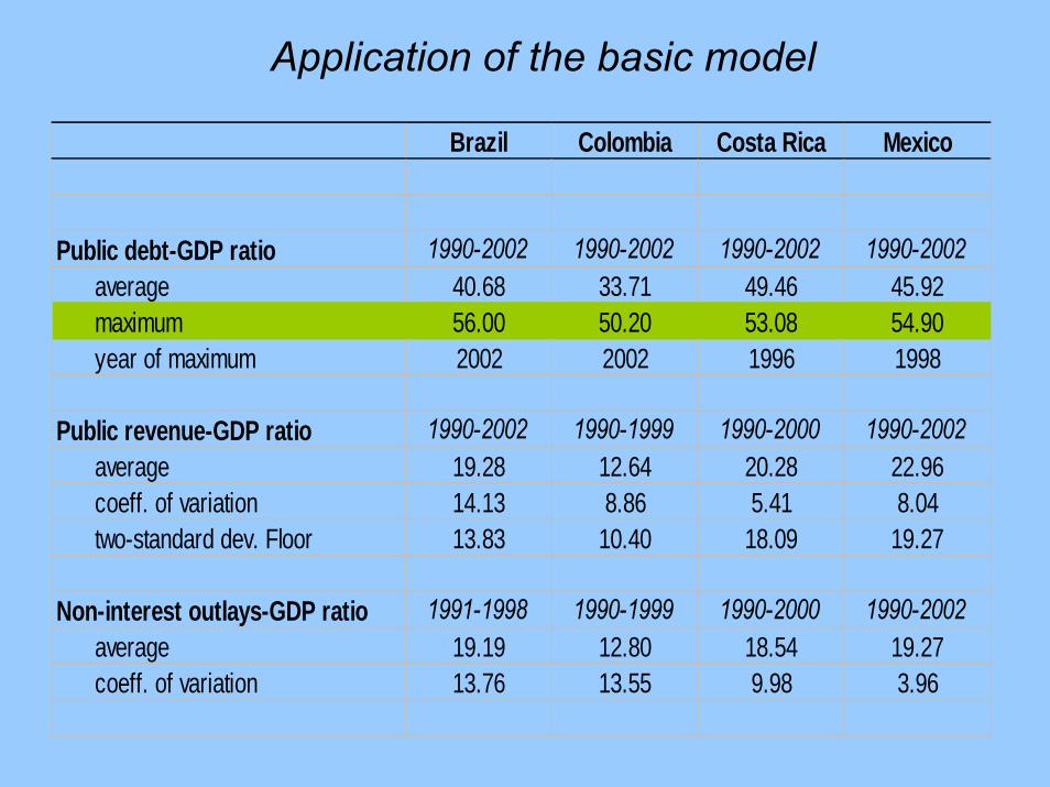
Application of the basic model

Brazil Colombia Costa Rica Mexico

Public debt-GDP ratio 1990-2002 1990-2002 1990-2002 1990-2002average 40.68 33.71 49.46 45.92maximum 56.00 50.20 53.08 54.90year of maximum 2002 2002 1996 1998

Public revenue-GDP ratio 1990-2002 1990-1999 1990-2000 1990-2002average 19.28 12.64 20.28 22.96coeff. of variation 14.13 8.86 5.41 8.04two-standard dev. Floor 13.83 10.40 18.09 19.27

Non-interest outlays-GDP ratio 1991-1998 1990-1999 1990-2000 1990-2002average 19.19 12.80 18.54 19.27coeff. of variation 13.76 13.55 9.98 3.96

Average & extreme “time to fiscal crisis:” Mexico

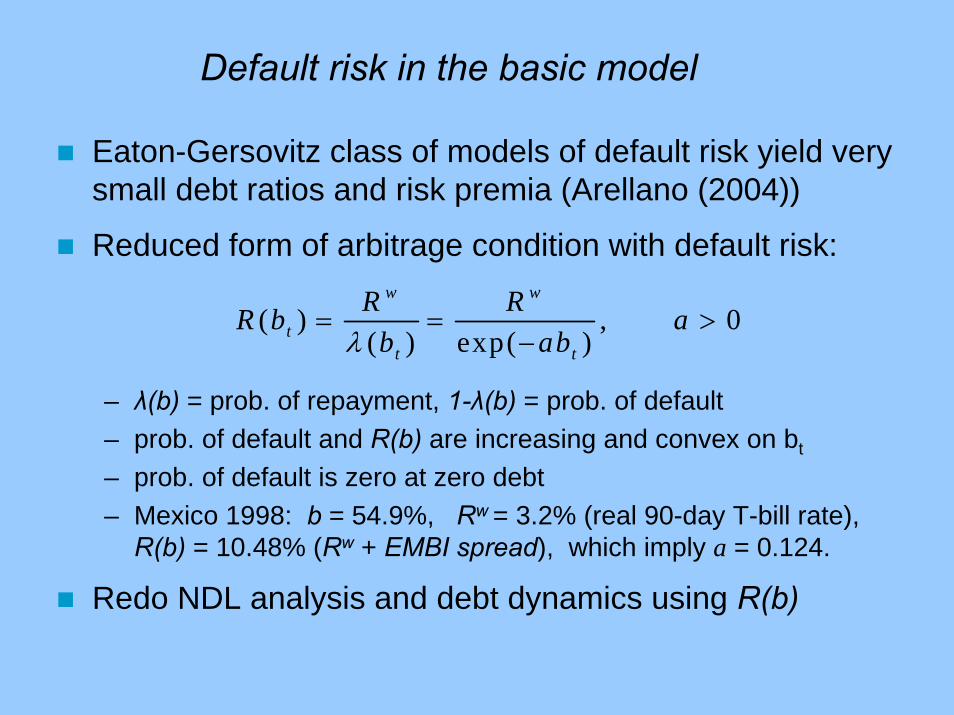
Default risk in the basic model

Eaton-Gersovitz class of models of default risk yield very small debt ratios and risk premia (Arellano (2004))

Reduced form of arbitrage condition with default risk:

– λ(b) = prob. of repayment, 1-λ(b) = prob. of default– prob. of default and R(b) are increasing and convex on bt

– prob. of default is zero at zero debt– Mexico 1998: b = 54.9%, Rw = 3.2% (real 90-day T-bill rate),

R(b) = 10.48% (Rw + EMBI spread), which imply a = 0.124.

Redo NDL analysis and debt dynamics using R(b)

( ) , 0( ) exp( )

w w

tt t

R RR b ab abλ

= = >−

Brazil Colombia Costa Rica Mexico

Benchmark NDLs with default risk 1/Natural debt limit 33.28 33.18 34.14 33.88Probability of default 4.04 4.03 4.14 4.11Default risk premium 4.31 4.30 4.42 4.39

NDLs in the growth slowdown scenario with default risk Natural debt limit 26.12 30.38 32.12 29.12Probability of default 3.18 3.69 3.90 3.54Default risk premium 3.37 3.93 4.16 3.76

NDLs in the growth slowdown scenario without default risk and risk free rate of 2.36 percentNatural debt limit 72.95 121.60 152.30 100.80

Required fiscal adjustment to support observed maximum debt ratios as NDLS 2/Natural debt limit 56.00 50.20 53.08 54.90Probability of default 6.70 6.03 6.36 6.57Default risk premium 7.35 6.57 6.95 7.20Implied minimum non-interest outlays 9.82 6.85 14.12 15.23 relative to average outlays -9.37 -5.95 -4.42 -4.04 in number of st. devs. 3.55 3.43 2.39 5.30

Notes: Calculations done as described in the text, using a risk free rate of 2.36 percent, which is the 1990-2002 average of the inflation-adjusted 90-day U.S. T-bill rate. 1/ Based on the benchmark values of growth rates and minimum revenue and outlays shown in Table 12/ Values of minimum outlays required to support maximum debt ratios shown in Table 1 as NDLs in the setting with default risk, using growth rates from the benchmark scenario.

Table 2. Natural Debt Limits with Default Risk

Long-run distributions of public debt and NFA

Public debt/GDP ratio NFA/GDP ratio