fishbones in jet plasmas with high icrh driven fast ions ... · fishbones in jet plasmas with high...
TRANSCRIPT

F. Nabais, D. Borba, M. Mantsinen, M.F.F. Nave, S.E. Sharapovand JET EFDA contributors
EFDA–JET–PR(04)65
Fishbones in JET Plasmas withHigh ICRH Driven Fast Ions
Energy Content

.

Fishbones in JET Plasmas withHigh ICRH Driven Fast Ions
Energy ContentF. Nabais1, D. Borba1, M. Mantsinen2, M.F.F. Nave1, S.E. Sharapov3
and JET EFDA contributors*
1Association EURATOM/IST, Av. Rovisco Pais, 1049-001 Lisboa, Portugal2Association EURATOM/TEKES, Helsinki University of Technology, Espoo, Finland
3 Association EURATOM/UKAEA Fusion Association, Culham Science Centre, Abingdon,Oxfordshire, OX14 3DB
* See annex of J. Pamela et al, “Overview of Recent JET Results and Future Perspectives”,Fusion Energy 2002 (Proc.19 th IAEA Fusion Energy Conference, Lyon (2002).
Preprint of Paper to be submitted for publication inPhysics of Plasmas

“This document is intended for publication in the open literature. It is made available on theunderstanding that it may not be further circulated and extracts or references may not be publishedprior to publication of the original when applicable, or without the consent of the Publications Officer,EFDA, Culham Science Centre, Abingdon, Oxon, OX14 3DB, UK.”
“Enquiries about Copyright and reproduction should be addressed to the Publications Officer, EFDA,Culham Science Centre, Abingdon, Oxon, OX14 3DB, UK.”

1
ABSTRACT
JET ICRH-only discharges with low density plasmas and high fast ions energy contents provided a
scenario where fishbones behaviour has been observed to be related with sawtooth activity: Crashes
of monster sawteeth abruptly changed the type of observed fishbones from low frequency fishbones
[3] to high frequency fishbones [2]. During periods between crashes, the type of observed fishbones
gradually changed in the opposite way. Two new fishbones regimes have been observed in
intermediate stages: Fishbones bursts covering both high and low frequencies and low amplitude
bursts of both types occurring simultaneously. Both sawtooth and fishbones behaviour has been
explained using a variational formalism.
1. INTRODUCTION
Bursts of MHD activity with the shape of “fishbones” have first been observed in 1983, on the
tokamak PDX during the injection of high power neutral beams [1]. These bursts were caused by a
rotating mode with toroidal mode number n=1 and dominant poloidal mode number m=1, which
caused the poloidal magnetic field fluctuations to oscillate in that peculiar way. The mode was
associated with the loss of energetic ions, which were expelled from the plasma core during the
bursts of MHD activity. This may not only reduce the auxiliary heating efficiency, but also the
maximum achievable β (kinetic pressure / magnetic pressure).
Towards the middle and the end of the eighties, two models were proposed to explain this
newfound MHD activity. Both assumed that the instability was caused by the presence in the plasma
of trapped fast particles precessing toroidally with frequency Dω , which for deeply trapped particles,
is given by
EqmrRω0
ωD= ,, (1)
where E is the particle energy, m the mass of the particle, r the minor plasma radius, R the major
plasma radius, q the safety factor, mZeB /0 =ω the gyrofrequency, and Ze is the particle charge. In
the first model, proposed by Chen, White and Rosenbluth [2], the inclusion of the fast particles
energy functional in the dispersion relation would create a new branch on its solution, which becomes
unstable when the fast particles beta hβ increases above a critical value. In this case, the mode is
created with the same frequency of the average precessional drift frequency Dω and it is
destabilized by resonant interaction with the trapped fast ions. The source of energy that drives the
mode unstable is then the spatial gradient of the fast ions distribution function. In the second model,
proposed by Coppi and Porcelli [3, 4], the trapped energetic ions destabilise an already existing
mode, which propagates in the thermal ion diamagnetic direction, and that was rendered marginally
stable by diamagnetic effects. The resonant interaction between the trapped particles and this mode
taps the source of energy for the instability, which is related to the pressure gradient of the plasma
bulk. In this model, the initial frequency of the fishbone instability is around the ion diamagnetic

2
frequency of thermal ions,
ω ≈ ω*i= 1
ZieniBr
dPi
dr- (2)
taken at the radius where the helicity of the perturbation matches that of the magnetic field, 1rr =
where 1r is the radius of the q=1 surface. Zie, ni, and Pi are the plasma thermal ions charge, density,
and pressure respectively. The two models for the fishbone instability were later found to correspond
to different limiting situations. The high frequency fishbones occurred for high values of the fast
ions’ beta hβ while the low frequency fishbones occurred for low values of, both regimes being
separated by a stable window. The two regimes merge when the diamagnetic frequency increases
to a sufficiently high value [5, 6]. In this paper, the higher frequency fishbones will be designed by
precessional (drift) fishbones and the lower frequency fishbones will be designated by diamagnetic
fishbones.
In JET plasmas diamagnetic fishbones are commonly observed; However, in ICRH-only
experiments carried out with low plasma densities and high contents of fast ions energy, MHD
activity in the range 45-75kHz, identified as precessional fishbones, was also observed [7]. In later
experiments, it was observed that the type of fishbones that appear in this kind of discharges were
related to the sawtooth stability. When sawteeth were unstable with frequent crashes precessional
fishbones were observed, but when sawteeth were stabilized and the crashes ceased, precessional
fishbones were gradually replaced by diamagnetic fishbones. Sawteeth crashes have already been
observed to affect fishbones activity. Indeed, it was reported that a sawtooth crash can temporarily
suppress the fishbone activity [8]. In JET experiments with high fast ion energy content another
effect was observed. Monster sawteeth crashes also suppress fishbones temporarily, but when
fishbone activity is resumed the type of observed fishbones changes from diamagnetic (before the
crash) to precessional (after the crash). The remainder of this paper is organized as follows. In Sec.
2 the existing theory is briefly reviewed, pointing out separately diamagnetic and fast particles
effects on fishbone activity. In Sec.3 the stability domains of sawteeth and fishbones activity,
including fast particle, diamagnetic and resistive effects are determined. In Sec.4 experimental
results showing the evolution of fishbones behaviour along a monster sawtooth cycle is presented.
The types of orbits of the ions resonating with the high frequency fishbones are shown in Sec.5.
The analysis and explanation of the experimental observations is done in Sec.6. Finally, conclusions
are presented in Sec.7.
2. THEORY REVIEW
2.1 DISPERSION RELATION
The common approach to analyse the stability of the internal kink mode taking into account the
effects of finite Larmor radius, resistivity and fast particles is by means of a variational formalism

3
[2], [9-13]. The plasma is assumed to be composed by a thermal background component treated
with resistive or ideal MHD and a hot component composed by the fast ions population, which is
dealt with a gyrokinetic formalism. Under these circumstances and assuming a large aspect ratio
circular cross-section, the internal kink mode behaviour is described by the following dispersion
relation [11-13].
δWMHD + δWHOT - = 0,8iΓ [(Λ3/2 +5)/4] [ω(ω - ω*i)]
/2
Λ9/4Γ[(Λ3/2-1)/4]ωΑ (3)
where,
Λ=i[ω (ω − ω*e)(ω - ω*i)]
1/3^
γR
, (4)
γR = S-1/3ωA is the resistive growth rate, S is the magnetic Reynolds number, ωA is the Alfven
frequency, is the electron diamagnetic frequency
ω*e =1
ene Br
dPe
dr, (5)
Pe and ne are the electron pressure and density respectively and
1 dTe
dr.ω*e= ω*e + 0.71^
eBr (6)
The Euler gamma functions in equation (3) come from the inertial layer and are evaluated at the
q=1 surface. is the usual isotropic functional for ideal internal kink modes [14] and
δWHOT =23/2mπ2
B2d(λB2/B0)
dE E5/2 K2 ω (δ/δ E + ω*/ωD)F2^
Kb(ωD -ω)
(7)
is the kinetic contribution coming from the fast ions distribution function F. Here, is the normalised
magnetic momentum, is a differential operator associated with the fast ion diamagnetic drift
frequency and K2 and Kb are elliptic functions arising from bounce averaging [10, 13].

4
2.2 DIAMAGNETIC EFFECTS
In the case of an ideal mode, and not considering diamagnetic or fast ions effects, the solution of
dispersion relation is
γI = - ωA δWMHD.. (8)
defines then the growth rate of the ideal internal kink mode associated with the minimized variational
energy. Including ion diamagnetics effects but keeping out resistive and fast ions effects, the
dispersion relation (3) becomes
γI + i[ω (ω-ω*i)]1/2 = 0, (9)
which has the analytical solutions,
ω =ω*i
2 2
ω*i– ( (2
-γI
1/2
. (10)
The behaviour of the solutions, represented in Fig.1, depends then on two frequencies, γI and ω*i.
When the diamagnetic frequency is zero, the ideal internal kink mode is a pure growing mode.
Diamagnetic effects tend to reduce the mode growth rate and at the same time the mode acquires a
real frequency. For values of i∗ω above a critical value that depends on the ideal growth rate
( Ii γω 2>∗ ), the internal kink mode is stabilized and two different branches become marginally
stable. The low frequency branch is the kink branch, which is now marginally stable, and the high
frequency branch is the ion branch. When including viscous effects as those provided by a resonant
interaction with trapped fast ions, the ion branch becomes unstable producing fishbone bursts while
the kink branch is damped. Nevertheless, the kink branch may also be unstable if resistive effects
are significant.
2.3 TRAPPED FAST IONS EFFECTS
The existence of the precessional (fishbone) branch is determined by the inclusion of the term
HOTWδ in the dispersion relation and can be predicted without diamagnetic or resistive effects. To
solve the dispersion relation when a fast ion population is present, it is necessary to specify the
distribution function. This is usually done for the case of a slowing down distribution in energy,
which is simpler than the Maxwellian case and produces qualitatively the same results. The numerical
solutions of the ideal dispersion relation with i∗ω = 0 are presented in [10]. For each set of parameters
(γI, βh) there are two different unstable solutions. The low frequency solution corresponds to the

5
kink branch and the high frequency solution corresponds to a new branch, the fishbone branch. The
growth rate of this mode goes to as goes to zero, but it becomes unstable for values of above a
critical value. This branch of the dispersion relation is an entirely new branch created by the inclusion
of the term , while on the contrary, the diamagnetic fishbones are caused by an already existing
branch, which can become unstable in the presence of fast ions.
2.4 FISHBONE REGIMES
As seen in sections II.2 and II.3, the existence of fishbones depends critically on the diamagnetic
frequency ω*i and on the fast ions beta βh. Diamagnetic fishbones can only be observed for values
of ω*i above a critical value while precessional fishbones can only be observed if βh is above a
critical value. For moderate values of ω*i (above the critical value) two different regimes of fishbones
can exist for different values of βh separated by a stable window [4, 5]. The diamagnetic fishbones
regime appears for low values of βh, while the precessional fishbones regime appears for high
values of βh. When increasing ω*i the stable window on βh narrows and for sufficiently high values
of ω*i it disappears. At this point the two fishbones regimes coalesce. The ideal unperturbed growth
rate γI plays here a role of a parameter and for increasing values of γI lower values of ω*i are
required in order to achieve the coalescence of the two fishbones regimes.
3. STABILITY DOMAINS
Considering a fast ion population produced by ICRF heating, the distribution in energy can be
approximated to a Maxwellian and, for on-axis heating, the population can be approximately
characterized by a single value of the normalized magnetic momentum λ ≡ µB0/E = 1,
F(E, λ, r) = n(r) δ(λ - 1)e -E/THOT . (11)
Here THOT is the temperature characterizing the Maxwellian distribution in energy. Introducing
this distribution function in the dispersion relation (3) and taking the average value of ωD on r, the
dispersion relation in the ideal limit can be written as [13]
- -i -γI
ωD ωD
ωωD
ωωD
ωωD
ωωD
ω*i
ωD
ω1_2
3_2
1_2
4_3
1_2
+ +βh
ε Z = 0 , (12)
and the threshold condition ω = real, i.e. the condition for which the stability of the mode changes,
is given by

6
-γ I = ωD
ωωD
ωωD
ωωD
ωωD
ω*i
ωD
ωωD
ω1_2
3_2
3_2
1_2
3_4
1_2
++ ReZ = 0 ,
-
(13)
with the corresponding value of given by,
-ωD
ωωD
ωωD
ω*i
ωD
ω1_2
5_2
3_
4
-
βh =εωA
ωDπ1/2
eω/ωD . (14)
If ω*i is of the same order of magnitude as <ωD>, then equation (13) has two solutions provided that
γI < γM, where γM is the maximum value that the right hand side of equation (13) can have, and βh
is a monotonic function of w.
If βh1 and βh2 are the values of βh corresponding to the solutions of equation (13) with βh1 < βh2,
then when the critical value βh1 is reached two different possibilities exist depending on the ratio
γI / ω*i. If γI / ω*i > 1/2, then this solution corresponds to the stabilization of the kink branch. If
γI / ω*i < 1/2 then βh1 is the threshold value for the stabilization of the ion branch.
The second threshold given by equations (13) and (14), βh2, corresponds to the threshold for the
fishbone branch destabilization. For βh > βh2 the precessional fishbone branch is unstable. In the
case of ω*i <<<ωD> the function βh is no longer monotonic and, when increasing βh the precessional
fishbone branch can be destabilized before the kink branch be stabilized.
If resistive effects are included, for values of γi sufficiently low depending on the Reynolds
magnetic number, the kink branch loses its ideal character and the resistive kink branch is unstable.
For plasmas containing high energy fast ions, finite orbit width effects over sawtooth stabilization
must also be taken account. It is known that an increase in the size of the trapped particles interacting
with sawteeth may reduce the efficiency of its stabilization [15]. Thus, if finite orbit width effects
are added, for sufficiently high values of THOT the stabilizing effect of the fast ions over the kink
branch may be lost and this branch may become unstable again. Since βh depends on THOT, there
must be a threshold value in βh above which the kink branch becomes unstable again. Note that the
same value of may be reached by increasing the fast particles density or the fast ions temperature
. If the threshold in is reached increasing the kink branch destabilization is not expected. So, when
considering finite orbit width effects, the threshold in should be replaced by a threshold in . The
resulting stability diagram is presented in Fig.2.
In region I the kink branch is unstable. Fast particles effects are too weak to stabilize the mode
( 1hh ββ < ) and the diamagnetic effects are also weak when compared with the ideal unperturbed
growth rate 21>∗iI ωγ . In region II the kink branch is stabilized by diamagnetic effects, but the
ion branch is now destabilized by fast ions. In region III the ion branch is still unstable and the kink
branch becomes also unstable due to resistive effects. In region IV the ion branch is stabilized

7
1hh ββ > , but the kink branch remains unstable due to resistive effects. In region V the precessional
branch is also destabilized by fast particles since the condition 2hh ββ > was reached. In region VI,
Iγ is high enough for resistive effects to be weak and the kink branch is stabilized by fast particles
effects. In region VII, if hβ is increased due to an increase in the fast ions’ temperature the kink
branch becomes unstable due to finite orbit width effects. If the increase in is due to an increase in
the fast ions’ density’ the kink branch remains stable. In region VIII, where , the low frequency
branch and the high frequency branch coalesce. For the precessional branch coalesces with the
kink branch (case represented in Fig.2) and for the precessional branch coalesces with the ion
branch. In both cases there is always one and only one unstable branch. The value of decreases
when increasing. In region IX all branches are stable.
4. EXPERIMENTAL RESULTS
In recent ICRH-only discharges on the JET tokamak with low plasma densities and high fast ion
energy contents, the fishbone behaviour was observed to change during the cycle of a monster
sawtooth.
Figure 3 shows the spectrogram of MHD activity for Pulse No:54300 and just the same sawteeth
and fishbone behaviour was observed in the subsequent Pulse No:54301, No:54305 and No:54306.
In these pulses, carried out under identical conditions, the regime of short sawtooth crashes appeared
always accompanied by precessional fishbones. As soon as the sawteeth were stabilized and the
frequent crashes stopped, precessional fishbones were gradually replaced by diamagnetic fishbones
until only diamagnetic fishbones existed.
Figure 4 shows a zoom where the temporal evolution of the fishbone regimes during a single
monster sawteeth is presented for Pulse No:54301.
At the beginning of the sawtooth free period, around t=9.2s, only precessional fishbones can be
observed. Later in the discharge precessional fishbones are replaced by “hybrid fishbones”, which
can be clearly seen around t=9.6s. The hybrid fishbones are a newly observed type of fishbones
that have characteristics of both the precessional and diamagnetic fishbones ranging all the way
from high to low frequencies. The amplitude of the hybrid fishbones bursts eventually starts
decreasing and they begin chirping down for a smaller range of frequencies. At some point, they
become precessional fishbones and at the same time diamagnetic fishbones appear in the low
frequencies. A new stage was reached where low amplitude bursts of both types of fishbones can be
observed simultaneously. This occurs just before t=9.8s. The precessional fishbones progressively
disappear until only diamagnetic fishbones remain. A monster sawtooth crash occurs just after
t=9.91s and the fishbone activity is suppressed, but after a short time (t=10.0s) precessional fishbones
reappear. The complete cycle is represented in Fig.5.
5. RESONANT IONS
One surprising feature of the precessional fishbones is their unexpectedly high frequencies. If the
mode was being destabilized by a population of trapped particles with a temperature around 1 MeV,

8
then one would expect averaged precessional drift frequencies below 50 kHz while the observed
MDH activity was in the range 50-70 kHz. To identify which particles were destabilizing the fishbone
branch, the CASTOR-K code [16] was used to calculate the resonant transference of energy between
a mode with a frequency of 70 kHz and an on-axis ICRH driven fast ions population with MeV,
which is around the value estimated for these pulses. The CASTOR-K used the eigenfunction
calculated by the MISHKA code [17] and simulations were carried out for a vast range of conditions.
Figure 6 shows the energy exchanged between the mode and a fast ion population peaked in the
centre and characterized by (on axis heating), MeV. As seen in this figure, the particles resonating
with the mode are not only trapped particles but also particles with potato orbits (Pϕ < 0). These
particles have a much higher precessional drift frequency ωD than the trapped particles, and also
contribute to the average precessional frequency of resonant particles <ωD>. Thus, this can explain
why the observed mode frequency is higher than the predicted by the average precessional drift of
trapped particles.
6. STABILITY ANALYSIS
6.1 INTRODUCTION
In the variational approach presented in section III, fishbone and sawtooth stability depends basically
on three parameters ( ihI ∗ωβγ ,, ), if resistive effects are not taken account. Resistive effects are
only important if the unperturbed mode is close to the marginal stability ( Iγ close to zero). For the
ideal internal kink mode, any change in the fishbones or sawtooth behaviour must be due to a
change in any of the three parameters ( ihI ∗ωβγ ,, ). Quantitative comparisons between the stability
diagram of Fig.2 and experimental results are very difficult. On one hand, the approximations used
in the dispersion relation and in the distribution function, and especially the fact that the radial
dependence of was not taken account, make the borders of the regions in the stability diagram
quite uncertain. Also the large size of the orbits may contribute to the uncertainty in the location of
the lines corresponding to and. On the other hand there is also an amount of uncertainty in the
values of ( ihI ∗ωβγ ,, ) calculated with experimental data. Thus, a qualitative analysis is more adequate
than trying to fit the calculated values of ( ihI ∗ωβγ ,, ) within the regions of the stability diagram.
6.2 PRECESSIONAL FISHBONES
In Pulse Nos:54300 to No:54305 small period sawteeth are always observed along with precessional
fishbones. This occurs when the plasma density is below a certain threshold [7], which, since the
plasma density is inversely proportional to the fast ions temperature [18], corresponds also to a
threshold in. Assuming that the occurrence of frequent sawteeth crashes are due to finite orbits
effects [19], then this regime corresponds to the region VII in Fig.2. When the plasma density
increases and the fast ions’ temperature decreases, sawteeth are stabilized by the fast particles but
precessional fishbones continue to be observed. This transition corresponds to crossing the pink
line in Fig.2 and moving from region VII to region VI. The growth rate of the mode causing
precessional fishbones has been calculated numerically [20].

9
6.3 HYBRID FISHBONES
During sawteeth free periods the q=1 surface expands as result of magnetic diffusion and the ideal
growth rate increases. At the same time the absence of crashes allows the background ions’ pressure
profile to peak. The diamagnetic frequency is mainly determined by the radial gradient of the
background ions’ pressure, so this means that when sawteeth are stabilized by fast ion effects, both’
and’ increase. It is possible to estimate the increase in the diamagnetic frequency through the sawtooth
free period. In similar pulses (No:47575 and No:47576, taken as reference), the frequency in the
laboratory frame ƒ*iLAB = ω*i/2π + ƒrot for the regime where frequent sawteeth crashes and
precessional fishbones were observed was calculated [7] and a value below 3kHz was obtained.
Since the initial frequency of diamagnetic fishbones is around ω*i, it can be observed from the
MHD spectrograms that ƒ*iLAB increases from a value below 3kHz at the beginning of the sawteeth
free phase to more than 10kHz when diamagnetic fishbones are first observed. After the appearance
of diamagnetic fishbones continues to increase reaching typically values around 20kHz when the
sawteeth free period is ended by a monster crash. This dramatical increase in the diamagnetic
frequency drives the whole system. The effect over the stability diagram of Fig.2 is that the blue
line (γI = ω*i/2) drifts upward and at the same time the dark green line (γI = γM) drifts downward.
The condition γI = ω*i/2 was reached first but the system remains in the region VI of Fig.2 and only
precessional fishbones are still observed. After that, the diamagnetic frequency continues to increase
and at some point the condition γI > γM is also reached. When this happens, the fishbone branch of
the dispersion relation coalesces with the ion branch (see Fig.8) and the region VIII.a in the stability
diagram of Fig.7 is reached.
The ion-fishbone branch is always unstable and, for a given value of ω*i, behaves like the fishbone
branch for high values of βh and like the ion branch for lower values of βh. If βh is high enough when
a fishbone burst is triggered, it begins as a precessional burst. During the burst fast particles are
expelled from the plasma core and βh decreases significantly. Thus, it is possible that βh reaches values
small enough for the mode behaviour change to that of a diamagnetic fishbone, as indicated in Fig.8.
If the condition MI γγ > was reached before the condition 2iI ∗< ωγ , then the unstable branch
would be the kink-fishbone branch. In this case, the precessional burst and consequent decrease in
βh would have caused the mode to behave like the unstable kink and a sawtooth crash would have
been observed.
Figure 9 shows the temporal evolution of Bθ for the hybrid fishbones. The hybrid burst is initiated
with fast oscillations in Bθ, at frequencies characteristic of the precessional fishbones. The amplitude
of the oscillations reaches a maximum and begins decreasing, but resonant fast particles continue
to be expelled from the core and continues decreasing. At some point is low enough for a new
source of energy to be tapped. This new source of energy, related with the bulk ions, allows the
amplitude of the oscillations to grow again but now they have the characteristics of a diamagnetic
fishbones with much slower oscillations in Bθ.
In Fig.10 it is shown that each fishbone event where the frequency chirps down from around
80kHz to 10kHz, is related to a single burst. The frequency of occurrence of hybrid fishbone bursts
~
~
~

10
is nearly the same as the precessional fishbones, which is not surprising since the trigger condition
is the same. On the other hand, the amplitude of the hybrid bursts is usually higher than that of the
precessional or diamagnetic fishbones. The reason for this is that the energy related to the bulk ions
is normally tapped before the amplitude of the precessional part of the hybrid fishbone reaches its
maximum. Thus the energy tapped from the bulk ions is added to the already existing energy
coming from the fast particles allowing higher amplitudes to be reached.
6.4 COEXISTENCE OF BOTH TYPES OF FISHBONES
A further increase in the diamagnetic frequency i∗ω and in the ideal growth rate Iγ causes the ion-
fishbone branch to gradually lose its precessional behaviour. At this intermediate point where none
of the behaviours is dominant, both types of fishbones can be triggered independently, but they
both can only reach small amplitudes. Small amplitude precessional fishbones do not cause
diamagnetic energy to be tapped as in the previous case and so both types of fishbones exist
independently.
Figure 11 shows the transition from the hybrid fishbone regime to the regime where both fishbone
types coexist. The amplitude of the precessional part of the hybrid bursts become so small that no
longer triggers the diamagnetic burst. At the same time, diamagnetic bursts appear in the low
frequencies. The events are not correlated and near t=9.06s it can be observed that three precessional
bursts occur during a single diamagnetic burst. Even after t=9.1s a closer analysis of the Bθ signal
show the presence of very small amplitude precessional bursts.
6.5 DIAMAGNETIC FISHBONES
The small amplitude precessional fishbones eventually disappear and only diamagnetic fishbones
remain. The reason for this is once again the increases in Iγ and i∗ω , which causes the ion-fishbone
branch to behave as the ion branch. It has also been suggested that Alfven eigenmodes may expel
fast particles from the plasma core [21] and in this case there would be a decrease in hβ which
would further push the mode behaviour towards the diamagnetic side. Since the branch is unstable,
the usual diamagnetic fishbone behaviour is observed.
Diamagnetic bursts are less frequent than the precessional ones and, as seen in Fig.11, both the
amplitude of the bursts and the initial mode frequency, which is around the diamagnetic frequency
ω*i, increase in time.
6. 6 MONSTER SAWTOOTH CRASH
Diamagnetic fishbone bursts cease when a monster sawtooth crash occurs. The usual explanation
for the occurrence of monster sawteeth crashes is related with an increase of the radius of the q=1
surface r1 [22]. As the safety factor on the axis decreases and increases during the sawtooth free
period, according to the Bussac model [14], the energy required to stabilise the m=1 oscillations
increases as r13. At a certain point, the stabilizing effect provided by the fast particles is no longer
sufficient to stabilize the mode and a crash occurs. An alternative explanation recently proposed for the
~

11
occurrence of monster crashes is based on the possibility that Alfven instabilities would cause a depletion
of stabilizing ions from the core of the plasma [21]. In terms of the stability diagram of Fig.7, for the
crash to occur the region VIII.c must be accessed, which requires the condition γI/ω*i > 1/2 to be
verified. This means that the depletion of resonant ions from the plasma core alone cannot explain
the crash, since the stabilising effect of the finite diamagnetic frequency could not be overcome.
The crash must then be caused by a rapid increase in the ideal growth rate γI related to the expansion
of the q=1 surface. However, it is possible that the number resonating fast particles is small before
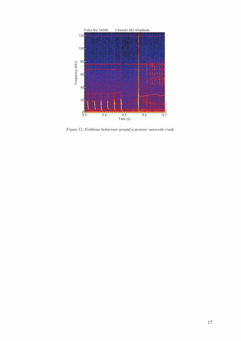
some crashes occur, as shown in Fig.12.
The diamagnetic bursts are suppressed almost one tenth of a second before the monster crash
occur, which suggests that the number of fast particles in the plasma core must effectively be small.
Nevertheless the suppression of diamagnetic fishbones just before the monster crash is not generally
observed. Some time after the crash the fast particle population is restored and precessional fishbones
are observed. Thus, the instability causing the fast particles to be expelled from the plasma core, if
there is any, must also have been suppressed by the sawtooth crash.
CONCLUSIONS
JET ICRH-only discharges with low density plasmas and high fast ion energy content provided a
new scenario where the stability of the internal kink mode in the presence of highly energetic ICRH
driven ions can be analysed. The qualitative behaviour of fishbones and sawteeth has been
successfully explained using a variational formalism. In this variational approach, the stability of
the ideal internal kink mode depends basically on three parameters ( ihI ∗ωβγ ,, ). A stability diagram
indicating the stability of each branch of the dispersion relation was drawn as a function of these
parameters. Precessional fishbones were observed in a regime of high hβ and low i∗ω . During
sawteeth free periods, precessional fishbones were observed to be gradually replaced by diamagnetic
fishbones. This is due to an increase in the diamagnetic frequency i∗ω and in the ideal growth rate
γI that causes the ion branch to coalesce with the fishbone (precessional) branch. The ion-fishbone
branch can behave as the ion branch or the fishbone branch depending on the parameters ( ihI ∗ωβγ ,, ).
The increase in i∗ω and γI, that occurs during sateeth free periods, push the behaviour towards the
ion branch type. When the precessional behaviour is slightly dominant, hybrid bursts that chirp
down both ranges of frequencies are observed. When none of the behaviours is dominant, low
amplitude bursts of both types occur simultaneously and independently. When the diamagnetic
behaviour is dominant, diamagnetic bursts are observed. A monster sawtooth crash flattens the
bulk ion profile and reduce the r1 radius, restoring low values of ω*i and γ1, and causing precessional
fishbones to occur. The fishbone cycle is then restarted by a monster sawtooth crash.
Aside from particles with banana orbits, the resonant ions include a minority of ions with potato
orbits that precess toroidally at higher frequencies ωD. This may account for the unexpectedly high
mode frequencies observed experimentally.
12
ACKNOWLEDGEMENTS
This work, supported by the European Communities and “Instituto Superior Técnico” under the
Contract of Association between EURATOM and IST, has been carried out within the framework
of the European Fusion Development Agreement. Financial support was also received
from”“Fundação para a Ciência e Tecnologia” in the frame of the Contract of Associated Laboratory.
The views and opinions expressed herein do not necessarily reflect those of the European
Commission, IST and FCT.
REFERENCES
[1]. K. McGuire et al. Phys. Rev. Lett. 50 891 (1983)
[2]. L. Chen, R. White and M. Rosenbluth, Phys. Rev. Lett. 52 1122 (1984)
[3]. B. Coppi and F. Porcelli, Phys. Rev. Lett. 57, 2272 (1986)
[4]. B. Coppi S. Migliuolo and F. Porcelli, Phys. Fluids–31, 1630 (1988)
[5]. Y. Zhang, H. Berk and S. Mahajan, Nucl. Fusion 29, 848 (1989)
[6]. B. Coppi et al. Phys. Rev. Lett. 63, 2733 (1989)
[7]. M. Mantsinen et al. Plasma Phys. Control. Fusion 42, 1291, (2000)
[8]. T. Krass et al. Nuclear Fusion 38, 807 (1998)
[9]. R. White et al. Phys. Fluids 26, 2958 (1983)
[10]. R. White, L.Chen, F. Romanelli and R. Hay, Phys. Fluids–28, 278 (1985)
[11]. R. White, P. Rutherford and P. Colestock, Phys. Rev. Lett. 60, 2038 (1988)
[12]. R. White, M. Bussac and F. Romanelli, Phys. Rev. Lett. 62, 539 (1989)
[13]. R. White, F. Romanelli and M. Bussac, Phys. Fluids B 2, 745 (1990)
[14]. M. Bussac et al. Phys. Rev. Lett. 35, 1638 (1975)
[15]. F. Porcelli–et al. Phys. Fluids B–4, 3017 (1992)
[16]. D. Borba and W. Kerner, J. Computational Physics 153, 101 (1999)
[17]. A.B. Mikhailovskii–et al. Plasma Physics Reports–10, 844 (1997)
[18]. T.H. Stix, Nuclear Fusion 15, 737 (1975)
[19]. F. Nabais et al. Submitted to Plasma Phys. Control. Fusion
[20]. N.N. Gorelenkov et al. EPS 2003, St. Petersburg, Russia (2003)
[21]. S. Barnabei–et al. Phys. Rev. Lett. 84, 1212 (2000)
[22]. C.K. Phillips et al. Phys. Fluids B 4 (7) 2155 (1992)

13
JG05
.37.
2c
VIII-C
I-S
IX-StableII-D
VII-S.P
VI-P
V-S,PIV-S
6
4
2
0
-2
-4
8
2 4 6 80 10ω*i (a.u.)
JG05
.37-
1c
Kink branchIon branch
ω*i = 2γI
γI
ω,γ
(a.u
.)
Figure 1: Solutions of the dispersion relation (9). Thegrowth rate (dashed lines) and real frequency (solid lines)of the mode are presented as function of the diamagneticfrequency …*i while the ideal growth rate γI plays therole of a parameter.
Figure 2: Stability diagram for the internal kink mode.In the regions labelled with S the kink branch responsiblefor sawteeth is unstable, in the regions labelled with Dthe ion branch responsible for diamagnetic fishbones isunstable and in the regions labelled with P the fishbonebranch responsible for precessional fishbones is unstable.For γI >γM the low frequency and high frequency branchescoalesce (region labelled with C).
Figure 3: Spectrogram of MHD activity for Pulse No:54300. Bothprecessional and diamagnetic fishbones activity are indicated with arrows.
1018
1
0
0
00 0
ND
e (m
-3 )
Time (s)
JG05
.
0
20
40
60
80
100
120
10 12 148 16Time (s)
JG05
.37.
3c
Diamagnetic Fishbones
Freq
uenc
y (k
Hz)
Pulse No. 54300 channel: 002 Amplitude
Precessional Fishbones
GiantSawteethCrashes

14
Figure 5: The fishbones cycle around a monster sawtoothperiod.
Figure 6: Energy exchanged between the fishbone branchof the internal kink mode with a frequency of 70 kHz anda population of on-axis ICRH driven fast ions with atemperature of 1MeV.
Figure 4: The fishbones cycle around the sawtooth crash in Pulse No: 54301.
Fre
quen
cy (
kHz)
0
20
40
60
80
100
120
9.6 9.8 10.0 10.29.49.2Time (s)
JG05
.37-
4c
Pulse No: 54301 channel: 002 Amplitude
Hybrid fishbones Both fishbonestypes coexist
Diamagnetic fishbones
Precessional fishbones Gaint sawtooth crash
Giantsawtooth
crash
Precessionalfishbones
Hybridfishbones
Both types of fishbones
Diamagneticfishbones
JG05
.37-
5c
0.015
0.010
0.005
0
-0.005
0.020
1000 20000 3000Energy (keV)
JG05
.37-
6c
0.000278840 / fish orbits 5
Nor
mal
ized
tor
oida
l can
onic
al m
omen
tum

15
Figure 8: Schematic diagram of the solution of thedispersion relation including diamagnetic and fast ioneffects. The smaller arrow indicates the evolution of themode behaviour during a hybrid burst, as fast ions areexpelled from the plasma core and hβ decreases.
Figure 9: Temporal evolution of Bθ for the hybrid fishbonein Pulse No:54300.
~
VIII.c- C:SP
VIII.b- C:DP
VIII.a- C:DP
VI-P
JG05
.37-
7c
Figure 7: Stability diagram for the internal kink mode.In the regions labelled with P the fishbone branchresponsible for precessional fishbones is unstable, in theregions labelled with C:DP the ion branch responsiblefor diamagnetic fishbones coalesces with the precessionalbranch and in the regions labelled with C:SP the kinkbranch responsible for sawteeth coalesce with theprecessional branch. The point X marks the state of theplasma when hybrid fishbones are observed.
JG05
.37-
8c
CoalescentIon-Fishbone
branch
precessionalbehaviour
Fishbonebranch
diamagneticbehaviour
_h decreasesduring the burst
Ionbranch
-3000
-2000
-1000
0
1000
2000
3000
12.551 12.553 12.555Time (s)
JG05
.37-
9c

16
4000
2000
0
-2000
-4000
9.54 9.58 9.629.50Time (s)
JG05
.37-
10c
120
100
80
60
40
20
09.54 9.58 9.629.50
Time (s)
JG05
.37-
11c
Freq
uenc
y (k
Hz)
Pulse No: 54301 channel: 002 Amplitude
100
80
60
0
120
8.9 9.1 9.3 9.5Time (s)
JG05
.37-
13c
Pulse No: 54300 channel: 002 Amplitude
40
20
Freq
uncy
(kH
z)
-4000
-2000
0
2000
4000
6000
8.9 9.1 9.3 9.5Time (s)
JG05
.37-
12c
~Figure 10: Temporal evolution of Bθ for the hybrid fishbones and correspondent MHD spectrogram.
Figure 11: Temporal evolution of Bθ and MHD spectrogram showing the transition to the diamagnetic fishbone regime.~
17
Pulse No: 54300 Channel: 002 Amplitude
0
40
100
80
60
20
120
9.4 9.5 9.69.3 9.7
Freq
uenc
y (k
Hz)
Time (s)
JG05
.37-
15c
Figure 12: Fishbone behaviour around a monster sawtooth crash.