fisheries centre research reports€¦ · persistent organic pollutants (pop), such as ddt, dioxins...

ISSN 1198-6727

Fisheries Centre Research Reports

2006 Volume 14 Number 3

On the Multiple Uses of Forage Fish:

From Ecosystems to Markets

A report to the Pew Institute for Ocean Science, University of Miami, Rosenstiel School of Marine & Atmospheric Science, Miami, FL

Fisheries Centre, University of British Columbia, Canada

s.mondoux

Text Box

Zeller, D., S. Booth, V. Lam, S. Lai, C. Close and D. Pauly. 2006. Global dispersion of dioxin: a Spatial Dynamic Model, with Emphasis on Ocean Deposition, p. 67-82 In: J. Alder and D. Pauly. (eds.). On the multiple Uses of Forage Fish: from Ecosystem to Markets. Fisheries Centre Research Reports 14(3).

On the Multiple Uses of Forage Fish: From Ecosystems to Markets edited by Jackie Alder and Daniel Pauly Fisheries Centre Research Reports 14(3) 120 pages © published 2006 by The Fisheries Centre, University of British Columbia 2202 Main Mall Vancouver, B.C., Canada, V6T 1Z4 ISSN 1198-6727

Fisheries Centre Research Reports 14(3) 2006

ON THE MULTIPLE USES OF FORAGE FISH: FROM ECOSYSTEMS TO MARKETS

edited by Jackie Alder and Daniel Pauly

CONTENTS

Page

DIRECTOR’S FOREWORD ....................................................................................................................................vii EXECUTIVE SUMMARY.......................................................................................................................................viii CHAPTER 1. FISHERIES FOR FORAGE FISH, 1950 TO THE PRESENT..........................................................................1 CHAPTER 2. HUMAN CONSUMPTION OF FORAGE FISH..........................................................................................21 CHAPTER 3. MARINE MAMMAL AND SEABIRD CONSUMPTION OF SMALL PELAGIC FISHES …...................................33 CHAPTER 4. FISHMEAL AND FISH OIL: PRODUCTION, TRADE AND CONSUMPTION.............................................................47 CHAPTER 5. GLOBAL DISPERSION OF DIOXIN: A SPATIAL DYNAMIC MODEL, WITH EMPHASIS ON OCEAN

DEPOSITION..................................................................................................................................67 CHAPTER 6. ECOSYSTEM MODELING OF DIOXIN DISTRIBUTION PATTERNS IN THE MARINE ENVIRONMENT ...............83CHAPTER 7. SYNTHESIS: ON THE MULTIPLE USES OF FORAGE FISHES................................................................103

A Research Report from the Sea Around Us Project, Fisheries Centre, UBC, to the Pew Institute for Ocean Science, University of Miami, Rosenstiel School of Marine & Atmospheric Science

120 pages © Fisheries Centre, University of British Columbia, 2006

FISHERIES CENTRE RESEARCH REPORTS ARE ABSTRACTED IN THE FAO AQUATIC SCIENCES AND FISHERIES ABSTRACTS (ASFA)

ISSN 1198-6727

Global dispersion of dioxin: A spatial dynamic model…, D. Zeller, S. Booth, V. Lam, S. Lai, C. Close and D. Pauly

67

CHAPTER 5

GLOBAL DISPERSION OF DIOXIN: A SPATIAL DYNAMIC MODEL, WITH EMPHASIS ON

OCEAN DEPOSITION5

Dirk Zeller, Shawn Booth, Vicky Lam, Sherman Lai, Chris Close and Daniel Pauly Fisheries Centre, Aquatic Ecosystems Research Laboratory (AERL), University of British Columbia.

2202 Main Mall, Vancouver, BC., V6T 1Z4, Canada [email protected]; [email protected]; [email protected]; [email protected];

[email protected]; [email protected]

ABSTRACT

The present study models the dispersion and deposition of airborne dioxin, a known carcinogen, on a global scale using atmospheric transport, with emphasis on ocean deposition. Human exposure is primarily through diet, and recent reporting of high levels in farmed seafood and fishmeal and fish oil products has increased concerns. A previously-published estimate of global dioxin production (13,100 kg·year-1) was allocated as airborne dioxin to terrestrial ½ x ½ degree GIS cells based on a linear relationship between dioxin production and GDP. Dioxin was then dispersed and deposited globally to both land—and water—GIS cells using two seasonal, 10-year time-averaged wind patterns. Our findings suggest that approximately one-third (4,214 kg·year-1) of globally-produced, and atmospherically- transported, total dioxins are annually deposited directly into marine environments. Based on published Characteristic Travel Distances and decay functions for dioxins, it would take over 270 days for the estimated total annual dioxin production to be deposited onto the Earth’s surface, and our wind dispersion patterns supported previous empirical observations of regional hot spots of marine dioxin loads (e.g., NE Atlantic). Comparison to field observations taken from terrestrial samples of deposited dioxins suggested relatively good fit, with measured concentrations on average being approximately 20% higher than modeled data suggested. It has previously been held that the majority of dioxin emissions is deposited near the source of emission, and only some dioxins are known to distribute globally. Our study suggested that the combination of average wind direction and predominantly coastal or near-costal location of high GDP areas facilitate the oceanic dispersion of over 30% of the estimated total dioxin production, which thus becomes directly available to the marine food webs.

INTRODUCTION

Persistent Organic Pollutants (POP), such as DDT, dioxins and PCBs, are chemicals which generally pose health risks to humans and animals (Foran et al., 2005). Typically, POP are of environmental concern because they are persistent, biomagnify and bioaccumulate in food webs, and have adverse effects on human health. Dioxins and furans are a class of POPs that are known carcinogens and have other sub-lethal effects in animals and humans (Anon., 2000). The general public first became aware of and concerned about these chemicals as a result of the use of Agent Orange as a dioxin containing defoliant used in Vietnam, and later due to industrial accidents such as in that Seveso, Italy (Baker and Hites, 2000).

The chemical structures of dioxins and furans are similar and consist of 75 polychlorinated dibenzo-para-dioxins (PCDD) and 135 polychlorinated dibenzofurans (PCDF). These two classes of POPs are usually combined in analysis when measurements are made on contaminated animal tissues, although in some

5 Cite as: Zeller, D., Booth, S., Lam, V., Lai, S., Close, C., Pauly, D. 2006. Global dispersion of dioxin: a spatial dynamic model, with emphasis on ocean deposition, p. 67-82. In: Alder, J., Pauly, D. (eds.) On the multiple uses of forage fish: from ecosystems to markets. Fisheries Centre Research Reports 14(3). Fisheries Centre, University of British Columbia [ISSN 1198-6727].

68 Global dispersion of dioxin: A spatial dynamic model…, D. Zeller, S. Booth, V. Lam, S. Lai, C. Close and D. Pauly

cases dioxin-like PCBs are also included. In the context of the present chapter, ‘dioxin’ is meant to include only the 75 congeners of dioxins and the 135 congeners of furans.

The congeners of dioxins are all lipophilic to varying degrees, and thus they bioaccumulate particularly well in oily tissues. However, they have different toxicology. Therefore, in order to assess the detrimental health effects brought about by exposure to the different forms, a relative ranking system is used in toxicological studies. This assigns toxic equivalency factors (TEFs) to the different forms relative to the most toxic congener, 2, 3, 7, 8-tetrachlordibenzo-p-dioxin (TCDD), which is given a TEF of one (Van den Berg et al., 1998). In this way, a total relative concentration in tissues can be assessed in terms of toxic equivalencies (TEQs). However, TEFs have been determined for only the 17 congeners of dioxin which are at least chlorinated in the 2,3,7,8 positions and of most toxicological concern (Buckly-Golder, 1999).

Dioxins are not deliberately produced for any specific human use, but rather are formed as incidental by-products during industrial processes, including the production of chlorinated chemicals, and as the result of combustion. Formation of dioxin during combustion is important globally, since some dioxins are known to disperse over long distances, primarily via atmospheric transport, although riverine inputs can be important in localized areas (Anon., 2004). Many dioxins are thought to be deposited relatively close to the source of emission (Brzuzy and Hites, 1996). While chemical sources of dioxin pollution (such as wood pulp bleaching) have resulted in localized environmental contamination, it is primarily through combustion that wide-spread contamination occurs due to atmospheric transport (Brzuzy and Hites, 1996).

For humans, approximately 90% of exposure is from dietary items, with fish, beef and dairy products being of prime concern (WHO, 1999). The World Health Organization (WHO) has set a Tolerable Daily Intake (TDI) of 1-4 picograms per kilogram bodyweight (Anon., 2000). The European Union’s limit for dioxin in fish is 4 pg·g-1 wet weight, while livestock and dairy products have a limit of 1-3 pg·g-1 lipid base (Lind, 2004).

A global model of general emissions and depositions of dioxin homologues noted that these two processes were not mass balanced (Brzuzy and Hites, 1996). Global estimates of annual dioxin depositions were thought to be approximately four times greater than estimated emissions (13,100 kg vs. 3,000 kg, Brzuzy and Hites, 1996). However, it has since been shown that atmospheric photochemical reactions of anthropogenic-produced pentachlorophenol (PCP), a common wood preservative, can produce dioxin, and this atmospheric formation of dioxin from PCP is thought to account for the imbalance (Baker and Hites, 2000).

The focus of our study is the presence of POPs, specifically dioxins, in small pelagic or ‘forage’ fish (herrings, sardines, anchovies, mackerels, etc; see Chapter 1), which are the main source for fishmeal and fish oil production for intensive aquaculture and poultry and swine production. Farmed salmon have been found to contain significantly elevated levels of dioxin compared to wild salmon, with European farm-raised salmon showing significantly higher levels of contamination than their North and South American counterparts (Hites et al., 2004). In order to account for the observed geographic differences in dioxin loads in farmed and wild-caught salmon (and other aquatic and agricultural products), we developed a GIS-based modeling approach to map the estimated global dispersion of dioxins via atmospheric transport. Given the lack of empirical measurements of ocean deposits of dioxins (Brzuzy and Hites, 1996), and the paucity of global dispersal model for POPs, we developed a global, spatially dynamic model for predicting global atmospheric dispersal and deposition of dioxins6. The aim was to predict the global dispersal of land-generated dioxin, and resultant deposits into the oceans, using global wind patterns and published travel-distance and deposition rates.

We utilized the global spatial resolution model of ½ x ½ degree spatial cells defined and used by the Sea Around Us project (SAUP, 2006). The basic methodology developed in this study rested upon several fundamental assumptions:

6 Note that, for the present, we did not include the effects of river run-off, which would increase coastal concentrations near major estuaries. Given the fast biogenic uptake of dioxins from water, this was assumed to have impacts primarily on ecosystems close to river deltas only.


69

• All dioxin was produced over land, and the amount based on published information;

• Spatial distribution of global dioxin production was directly related to level of economic activity of any given area, i.e., spatial dioxin production was assumed to be proportional to GDP;

• Dioxin dispersal was by atmospheric transport, driven by and influenced by average wind patterns in the lower atmosphere; freshwater run-off was not explicitly considered; and

• Rate of deposition of dioxin to the earth surface (land or water) followed published relationships for characteristic travel distances for dispersion, but included simulation of diffusion. We did not differentiate between wet and dry deposition.

The resultant estimate of global annual concentration of dioxin entering the world’s marine systems at the ½ x ½ degree resolution via atmospheric dispersion was used as input parameter into marine systems in the trophic modeling undertaken in other sections of this report.

METHODS

Global dioxin emission distribution

As starting position for our modeling simulations, we took the estimated mean total global deposition of dioxin (chlorinated dioxins and dibenzofurans) from the atmosphere of 13,100 ± 2,000 kg·year-1 as derived by Brzuzy and Hites (1996), and assumed this amount corresponded to the annual global production of dioxins by all sources. Hence, this was thought to also include those forms of dioxin that are known to form in the atmosphere via photochemical synthesis from pentachlorophenol (Baker and Hites, 2000). We distributed this total estimated annual dioxin load to all global land cells (½ x ½ degree) using the assumption of linear relationship between GDP and dioxin production (Baker and Hites, 2000).7 Global, spatialized GDP data were based on Dilley et al. (2005). It was assumed that the spatially distributed dioxin amounts were fully airborne above their assigned ½ x ½ degree land cells at the start of the dynamic dispersal phase. For technical details of the global dispersion model, see Appendix 1.

Simulated dispersion and deposition of airborne dioxin

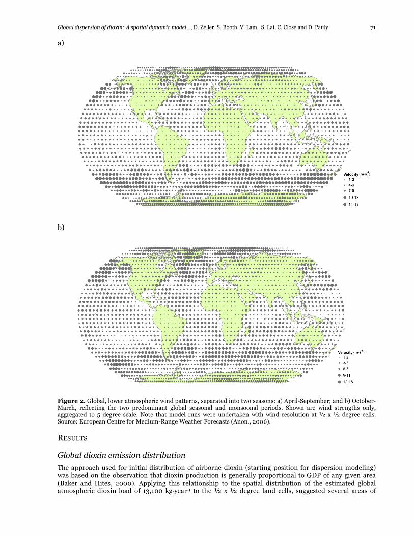
Dioxin was dispersed from its starting distribution in the atmosphere above land cells by modeling atmospheric transport driven by global lower atmosphere wind patterns. Two global seasonal wind patterns, representing the two main global seasonal and monsoonal periods (April-September and October-March), were obtained from the European Centre for Medium-Range Weather Forecasts (Anon., 2006). We averaged these data for the 1990-2000 time period, and recomputed the original vector-based data for present use into direction and velocity components by season (Figures 1, 2). The two seasonal global distribution models (April-September and October-March) were run separately, and thus half of the global estimate of dioxin production of 13,100 kg·year-1 (Brzuzy and Hites, 1996) was dispersed in each seasonal run, and the final deposited amounts from each run were combined to derive annual total deposits. Hence, we assumed equal dioxin production potential for each season. The model of dioxin dispersal included the use of a wind-speed dependent characteristic travel distance for dioxin to derive an effective decay rate and resultant deposition (Bennett et al., 1998; Beyer et al., 2000). We also incorporated diffusion, using published diffusion coefficient in air for dioxins (Chiao et al., 1994).

Each seasonal model was run for 200,000 time steps (each time step representing 60 s in real time, see Appendix 1), which is equivalent to approximately 139 days or 4½ months in real-time, after which over 99% of the seasonal atmospheric dioxin had been deposited into either land or water cells. Subsequently, the outputs from the two seasonal models were combined to derive the total annual dispersion and deposition of dioxin to both land and ocean cells.

7 Baker and Hites (2000) found a close correlation (r² = 0.8) between the logarithm of GDP and the logarithm of annual dioxin production per country examined. As their log-log relationship suggested a slope of close to unity, we assumed a linear relationship between GDP and dioxin production.


a)

b)

Figure 1. Global, lower atmospheric wind patterns, separated into two seasons: a) April-September; and b) October-March, reflecting the two predominant global seasonal and monsoonal periods. Shown are wind direction only, aggregated to 5 degree scale. Note that model runs were undertaken with wind resolution at ½ x ½ degree cells. Source: European Centre for Medium-Range Weather Forecasts (Anon., 2006).


71

a)

b)

Figure 2. Global, lower atmospheric wind patterns, separated into two seasons: a) April-September; and b) October-March, reflecting the two predominant global seasonal and monsoonal periods. Shown are wind strengths only, aggregated to 5 degree scale. Note that model runs were undertaken with wind resolution at ½ x ½ degree cells. Source: European Centre for Medium-Range Weather Forecasts (Anon., 2006).

RESULTS

Global dioxin emission distribution

The approach used for initial distribution of airborne dioxin (starting position for dispersion modeling) was based on the observation that dioxin production is generally proportional to GDP of any given area (Baker and Hites, 2000). Applying this relationship to the spatial distribution of the estimated global atmospheric dioxin load of 13,100 kg·year-1 to the ½ x ½ degree land cells, suggested several areas of


likely high atmospheric dioxin concentration due to high local production of dioxins (Figure 3). These were dominated by eastern North America, Europe, South Asia (particularly the Indian subcontinent), and East Asia (China, Japan and South Korea).

Figure 3. Estimated spatial distribution pattern of global dioxin production, based on the published linear relationship between dioxin production and GDP (Baker and Hites, 2000).

Dispersion and deposition

The dispersion, diffusion and decay model using published characteristic travel distance and diffusion coefficient for dioxins (Chiao et al., 1994; Bennett et al., 1998; Beyer et al., 2000), resulted in 99.14% of airborne dioxin being deposited during the two seasonal runs of 200,000 time steps each (~139 days real time each (Table 1)). Thus, the annually-produced 13,100 kg of dioxin would take approximately 278 days (2 • 139 days) for over 99% to be deposited onto the earth’s surface. However, atmospheric deposition is not a linear process; the majority of dioxin is deposited within a much shorter time period, with approximately 50% and 75% of airborne dioxin deposited within 5 and 13 days of emission, respectively (Figure 4). Given the terrestrial sources and the non-linear deposition function, the distribution between land and ocean deposition was uneven, with 67% and 32% of deposited dioxin, respectively (Table 1). Thus, our model suggests that, on average, approximately one third of globally-produced dioxins are deposited directly in the ocean due to atmospheric transport.

Table 1: Summary of seasonal and total dispersion and deposition of dioxins based on global atmospheric dispersal and reported atmospheric decay (deposition) functions.

Amount of dioxin after simulation runsa (kg) Time period

Initial dioxin in air

(kg) Air Land Ocean

Percentage of airborne

dioxin deposited

April-September 6,550 62.2 4,572.3 1,915.5 99.05

October-March 6,550 49.8 4,201.3 2,298.9 99.24

Annual combined 13,100 112.0 8,773.6 4,214.4 99.14

Percentage of total dioxin deposit

66.97 32.17

a Seasonal runs were for 200,000 time steps, being approximately 139 days real-time each, while annual totals equate to 278 days (2 • 200,000 time steps).


73

Figure 4. Amount of dioxin in the air, and deposited into the ocean and land cells over time, based on the dispersion and diffusion model with the two seasonal models pooled.

Spatial patterns of dispersion

Based on the two seasonal, 10-year average wind field patterns, the global distribution of modeled dioxin deposition suggested several terrestrial and oceanic hot spots (Figure 5). Specifically, large parts of North America, most of central, northern and Eastern Europe, as well as much of the Indian sub-continent and East Asia have high terrestrial depositions of dioxins (Figure 5a). Under the assumption that the published characteristic travel distance and effective decay rate of dioxins as measured under terrestrial conditions also applied to oceanic conditions, it suggested that many ocean areas around the world may also have relatively high dioxin loads. These include the northeast and west Atlantic, Caribbean, Mediterranean, northern Indian Ocean, and large parts of the north-western Pacific and South China Seas (Figure 5b). However, several areas of relatively low concentration of dioxins also emerged, specifically parts of the west coast of South America and northern parts of the west coast of North America (Figure 5b). Our model suggested that final concentrations of deposited dioxins in our ½ x ½ degree model cells ranged from as low as 4.5·10-40 g·km-2 to as high as 7.5 g·km-2 for marine environments, with the April-September seasonal run showing a larger range of concentrations than the October-March season (Table 2).

Terrestrial environments had concentrations from 7.11·10-61 g·km-2 to 55.39 g·km-2, with the larger range of concentrations also observed during the April-September period (Table 2). Global annual average concentrations were 1.25·10-2 and 4.4·10-2 g·km-2 for marine and terrestrial areas, respectively (Table 2). Note, however, the difference in scale between terrestrial and oceanic deposition (Figure 5a,b), confirming that, globally, most dioxins were deposited on land, close to their area of production (Brzuzy and Hites, 1996).

Table 2: Minimum, maximum and mean deposited dioxin concentrations per ½ x ½ degree cells, separated by season and land-versus-ocean cells. Deposited dioxin concentration per cell (g·km�²)

Water Land

April-September October-March Annual

April-September October-March Annual

Minimum 4.46·10ֿ40 2.02·10ֿ39 8.40·10ֿ31 7.11·10ֿ61 1.51·10ֿ33 1.51·10ֿ33 Maximum 7.46 3.21 7.54 55.39 6.77 55.80 Mean 5.65·10³ֿ 6.81·10³ֿ 1.25·10²ֿ 2.26·10�² 2.14·10²ֿ 4.40·10²ֿ


a)

b)

Figure 5. Global distribution of modeled dioxin deposition, based on the two seasonal, 10 year average wind field patterns combined, showing spatial distribution (a) on land, and (b) in the ocean (note difference in scales).

Validation of spatial dispersion

In order to determine how well our dispersal and deposition algorithm replicated real-world distribution and deposition of airborne dioxins, we compared 107 empirical field measurements taken from soil samples reported by Brzuzy and Hites (1996) with the values predicted from our model runs for the same spatial coordinates. As no empirical dioxin measures exist for seawater samples, we had to rely on terrestrial validations only. Due to our spatial resolution of ½ x ½ degree cells, 11 model cells were coastal


75

in location, i.e., did not correspond to land locations. These samples were excluded from the present comparison, resulting in 96 actual measures being compared between modeled results and the corresponding empirical terrestrial field measurements. This comparison (Figure 6a) showed a significant positive relationship between empirical and model results with a moderate fit (p<<0.001, R2=0.203). On average, empirically-measured dioxin concentrations in soil were 20.6% higher than our modeled results suggested. The observed relationship could likely be improved by weighing the initial GDP-related distribution of dioxin production by an indicator of environmental and pollution standards by country, as our results suggest possible differences related to these standards. For example, European countries, which have relatively well established pollution mitigation standards, had measured values generally lower than suggested by our model, while North American countries (Mexico, Canada and USA), with their more diverse range of environmental standards, showed more variable patterns. The few available empirical measurements from African countries suggested our model slightly underestimated their empirical dioxin loading (Figure 6b), possibly because our assumptions about dioxin being linked to GDP did not account for the dioxins produced by extensive burning of vegetation in many parts of Africa (e.g., Cahoon et al., 1992). Furthermore, it has been suggested that by replacing the seasonally-averaged wind patterns by monthly patterns and simulations, as is commonly done in atmospheric chemistry, a better fit between empirical deposition and modeled results might be obtainable (D. Mauzerall, University of Princeton, pers. comm.).

Figure 6. Model validation comparison: a) between empirically-measured terrestrial dioxin depositions based on Brzuzy and Hites (1996) and the geographic equivalent model results from the present dispersal and deposition model; b) a subset of (a) showing data from European (■), North American () and African (▲) countries only. The significant regression for the whole data set with moderate fit (p<<0.001, R2=0.203, n= 96), is also shown. Data were log-converted to account for large number of small values. Note that field measurements exist only for terrestrial locations.


CONCLUSION

To our knowledge, this is the first attempt to model the dispersion and deposition of dioxins on a global scale using atmospheric transport. Our findings suggest that:

• Approximately one-third (4,214 kg) of globally-produced, and atmospherically-transported total dioxins are annually deposited directly into marine environments;

• Based on published Characteristic Travel Distances and decay functions for dioxins, it would take over 270 days for the estimated total annual dioxin production of 13,100 kg to be deposited onto the earth surface;

• Our wind dispersion patterns supported previous empirical observations of regional hot spots of marine dioxin loads (e.g. NE Atlantic); and

• Comparison to field observations taken from terrestrial samples of deposited dioxins suggested relatively good fit, with measured concentrations being on average approximately 20% higher than modeled data suggested.

It has previously been held that the majority of dioxin emissions appear to be deposited in climate zones near to the source of emission, and only some dioxins are known to be distributed globally, due to long-range atmospheric transport (Brzuzy and Hites, 1996). While fundamentally concurring with this observation, our study suggested that the combination of average wind direction and predominantly coastal or near-costal location of high GDP areas facilitates the oceanic dispersion of dioxins. This caused over 30% of the estimated total dioxin production to be deposited directly into the marine environment during our simulations, thus becoming directly available to the marine food web.

REFERENCES Anon .2000. Air quality guidelines for Europe, 2nd edition. World Health Organization, Copenhagen, Denmark, 273 p.

Anon. 2004. Codex committee on food additives and contaminants: position paper on food additives and contaminants. Food and Agriculture Organization of the United Nations and World Health Organization, Rome, Italy, 17 p.

Anon. 2006. The European Centre for Medium-Range Weather Forecasts: data from the ECMWF 40 Years Re-Analysis. [Available at: http://data.ecmwf.int/data/index.html. Accessed February, 2006].

Baker, J.I. , Hites, R.A. 2000. Is combustion the major source of Polychlorinated Dibenzo-p-dioxins and Dibenzofurans to the environment? A mass balance investigation. Environmental Science and Technology 34, 2879-2886.

Bennett, D.H., Mckone, T.H., Matthies, M., Kastenberg, W.E. 1998. General formulation of characteristic travel distance for semivolatile organic chemicals in a multimedia environment. Environmental Science and Technology 32, 4023-4030.

Beyer, A., Mackay, D., Matthies, M., Wania, F., Webster, E. 2000. Assessing long-range transport potential of persistent organic pollutants. Environmental Science and Technology 34, 699-703.

Brzuzy, L.P. and Hites, R.A. 1996. Global mass balance for Polychlorinated Dibenzo-p-dioxins and Dibenzofurans. Environmental Science and Technology 30, 1797-1804.

Buckly-Golder, D. 1999. Compilation of EU Dioxin Exposure and Health Data. Report to European Commission DG Environment (97/322/3040/DEB/E1). AEA Technologies PLC, Abingdon, U.K., 629 p.

Cahoon, D.R., Stocks, B.J., Levine, J.S., Cofer, W.R., O'Neill, K.P. 1992. Seasonal distribution of African savanna fires. Nature 359, 812-815.

Chiao, F.F., Currie, R.C. McKone, T.E. 1994. Final draft report: Intermediate transfer factors for contaminants found in hazardous waste sites: 2, 3, 7, 8-Tetrachlorodibenzo-p-Dioxin (TCDD). Risk Science Program (RSP), Department of Environmental Toxicology, University of California, Davis, California, USA, 30 p.

Dilley, M., Chen, R.S., Deichmann, U., Lerner-Lam, A.L., Arnold, M. 2005. Natural disaster hotspots: a global risk analysis. CIESIN and World Bank (unpublished data), Washington, DC. 145 p.

Foran, J.A., Carpenter, D.O., Coreen Hamilton, M., Knuth, B.A., Schwager, S.J. 2005. Risk-based consumption advice for farmed Atlantic and wild Pacific salmon contaminated with dioxin and dioxin-like compounds. Environmental Health Perspectives 113, 552-556.

Hites, R.A., Foran, J.A., Carpenter, D.O., Coreen Hamilton, M., Knuth, B.A., Schwager, S.J. 2004. Global assessment of organic contaminants in farmed salmon. Science 303, 226-229.

Lind, G. 2004. REACH-The only planet guide to the secrets of chemical policy in the EU: What happened and why? European Parliament (Inger Schöling, Member of the Greens/European Free Alliance), Brussels, Belgium, 145 p.


77

Sea Around Us Project . 2006. A global database on marine fisheries and ecosystems. [Available at www. seaaroundus.org. Accessed 17 July 2006].

Van den Berg, M., Birnbaum, L., Bosveld, A.T.C., Brunström, B., Cook, P., Feeley, M., Giesy, J.P., Hanberg, A., Hasegawa, R., Kennedy, S.W., Kubiak, T., Larsen, J.C., van Leeuwen, F.X.R., Djien Liem, A.K., Nolt, C., Peterson, R.E., Poellinger, L., Safe, S., Schrenk, D., Tillitt, D., Tysklind, M., Younes, M., Wærn, F., Zacharewski, T. 1998. Toxic equivalency factors (TEFs) for PCBs, PCDDs and PCDFs for humans and wildlife. Environmental Health Perspectives 106, 775-792.

World Health Organization. 1999. Dioxins and their effects on human health. [Available at: http://www.who.int/mediacentre/factsheets/fs225/en/index.html. Accessed: January 2006].


APPENDIX

Technical details of the spatially dynamic model for predicting wind-driven global distribution of dioxin

Aims

To predict the global wind-driven dispersion of airborne dioxin and to determine the amount of dioxin deposited into the ocean and on land.

Methodology

To estimate the global dispersion and deposition of dioxin in the ocean and on land, we developed a spatially dynamic model with two driving parameters: a) anthropogenic dioxin production set proportional to GDP; and b) global wind patterns as the primary means of long-distance dispersal of dioxin. Details of each parameter and methodology are explained in the later sections of this document.

We initiated the simulations with terrestrially-produced, airborne dioxin distributed proportional to GDP to all land cells in a global, spatial grid system with ½ x ½ degree resolution, based on the global ½ degree cell system of the Sea Around Us project (given the spherical nature of the globe, this implied that cell surface areas and east-west dimensions varied with latitude).

Since wind direction can vary globally between seasons (e.g., tropical monsoons), we separated the wind data into two time periods: April-September and October-March. We assumed equal production of dioxin throughout the year, thus the initial starting amount of airborne dioxin (13,100 kg) was separated into two halves (6,550 kg) and assigned to each seasonal time period.

A spatially dynamic model was developed using Visual Basic (Microsoft vb.net) to predict the amount of dioxin transferred to neighbouring cells. We iterated the initial state of dioxin through all the cells in the world, applying two driving mechanisms: diffusion (independent of wind) and dispersion (wind-dependent). Within the dispersion module, a decay function was applied to account for deposition onto the earth surface (land or water). These mechanisms distributed dioxin during each simulation iteration (time-step) to a new model state, which has some dioxin in each cell remaining in the air, and some having been deposited (decayed) onto the ground or water. Once dioxin was deposited, it no longer was exposed to the distribution mechanisms. This new state was then reapplied to the distribution mechanisms, until ≥ 99% of the initial airborne dioxin had been deposited onto land/water.

Data

Below is a table that outlines the basic input data.

Table A1. Basic input data for spatial model

Data Sets Type Purpose Source Data Format (Resolution)

Average N-S wind component at 10m (April–Sept, 1990-2000) Data Grid

Wind acts as dioxin dispersal force. Data were decomposed into wind direction and speed.

ECMWP1 NetCDF (2.5 degree)

Average E-W wind component at 10m (April–Sept, 1990-2000)

Data Grid - ECMWP1 NetCDF (2.5 degree)

Average N-S wind component at 10m (Oct–March, 1990-2000) Data Grid - ECMWP1 NetCDF

(2.5 degree) Average E-W wind component at 10m (Oct–March, 1990-2000)

Data Grid - ECMWP1 NetCDF (2.5 degree)

Initial concentration of dioxin in the atmosphere

Interpolated from GDP

Initial amount of dioxin in the air. Global total based on literature (Brzuzy & Hites, 1996)

SAUP2 Raster

(2.5 arc minutes)

World Table Access Percent water/land in each ½ degree cell

SAUP Access table (0.5 degree)

1 European Center for Medium Range Weather Forecasting. 2 GDP data based on Dilley et al. (2005)


79

Dioxin

The amount of dioxin generated globally was set as 13,100,000 g (Brzuzy and Hites, 1996). We assigned the total amount of dioxin to the air above all land cells throughout the world in proportion to the Gross Domestic Product (GDP) of each cell, based on the documented correlation between dioxin production and GDP (Baker and Hites, 2000). The GDP data had a resolution of 2.5 arc minutes (Dilley et al., 2005) and was adjusted to 0.5 degree cells by interpolation. The interpolation was carried out using the Nearest Neighbour algorithm in ArcGIS.

Dioxins, like all airborne chemicals, are subject to simple diffusion. We simulated diffusion of dioxin based on the published diffusion rate for 2,3,7,8-TCDD dioxin (Chiao et al., 1994),. Diffusion was the first operation applied in each computational time step to distribute dioxin between cells.

The modeling of dioxin dispersion based on wind speed, wind direction and characteristic travel distance was the second operation undertaken in each time step. Deposition of dioxin from air to land/ocean cells was accounted for with an exponential decay model (Bennett et al., 1998). We applied the proportion of marine versus terrestrial environment per cell to the allocated dioxin deposition per cell to derive land and ocean deposition amounts.

Wind

The data consisted of global monthly daily means of east-west and north-south wind component data (m·s-

1) from the ‘40 years Re-analysis Database’ of the European Center for Medium Range Weather Forecasting (ECMWP)1. These data were further averaged over the 1990 to 2000 time period into two sets of values one set representing April to September and one set representing October to March. These values were applied to each 2.5-degree cell for each time period. The resulting NetCDF files were then converted into raster files and decomposed into wind magnitude and wind direction using the DECOMP module in IDRISI. The 2.5-degree resolution of the original wind data was converted to 0.5-degree cell resolution via the interpolation method of Nearest Neighbour.

In this document, µ is the wind speed in m·s-1 and θ is the wind angle (0 degrees being due east).

We are aware that the temporal resolution provided by 6-month wind fields is low, and will be re-doing these analyses using monthly wind grids, as is the standard in atmospheric chemistry.

Parameter Estimation

Latitude

Latitude (lat) is defined as the current latitude in the center of a given cell. The most northerly and southerly row of cells have the latitude of 89.75 and -89.75 degrees, respectively. The cell latitude for the two rows at the equator is 0.25 and -0.25 degrees, for north and south respectively.

Time step

The computational time step (ts) was defined as the amount of time allowed for dioxin to travel per iteration. We chose a time step that was less than the time taken for the highest wind speed (µmax) to cross the smallest cell dimension (cdmin):

max

min

µcdts ≤

This was done to ensure that ts was not large enough for dioxin to move past any neighbouring cells in any one iteration. Given the latitudinal differences in east-west cell dimensions of the ½ x ½ degree cells used,

1 ECMWP website: http://data.ecmwf.int/data/index.html


the smallest dimension was taken as the east-west dimension for cells at 89.75 degree latitude (1320 m), with fastest global wind speed from both seasonal wind fields (21.3 m·s-1). Thus, minimum time needed at 89 degree was 61.97 s (i.e., 1320 m / 21.3 m·s-1). We reduced this to a standardized ts of 60 s for our runs. Thus, the number of time steps represents minutes in real time.

Characteristic travel distance

The characteristic travel distance (CTD) for a chemical is defined as the distance required for its concentration to be reduced to 1/e (~37%) of its initial value via deposition (Bennett et al., 1998; Beyer et al., 2000). The amount of dioxin in the air of a particular cell was reduced by both deposition and transport (diffusion and dispersion) to neighbouring cells. The CTD of dioxin for the most toxic congener 2,3,7,8-tetrachlorodibenzo-p-dioxin in air is 810 km at wind velocity of 4 m·s-1 (Beyer et al., 2000), and was chosen as the dispersion rate for this model.

Cell distance

The cell distance (d) is the coordinal distance of one of the 720 equatorial cells of 0.5 degree, and is also related to the circumference of the earth (40,075.16 km/720 cells).

Wind distance

Wind distance is the distance the wind in a given cell travels during one time step. Wind distance was defined as:

tsts

!= µµ

where µ represents the wind speed and ts represent the time step.

Diffusion

As noted above, diffusion is first applied to every cell. The amount of dioxin diffused in each time step was calculated as:

tiodiffusedRaodiffused DND !=

Where No is the amount of dioxin in the air in a cell at the beginning of each time step, and DDiffused Ratio was calculated as:

)cos(

2

latd

tsDiffCoefD tiodiffusedRa

!

!!=

Where lat is the latitude of the current cell at the center of that cell, ts is the time step, and DiffCoef is the diffusion coefficient of dioxin equal to 0.42 m2·day-1 or 4.86 • 10-6 m2·s-1 (Chiao et al., 1994).

Ddiffused was then divided into 4 equal values (i.e., 25% each), and was allocated to the air of the neighbouring cells in the cardinal directions (north, east, south and west) of the originating cell only. This diffused dioxin was then available for the next iteration in the receiving cells.


81

Decay (deposition)

The dioxin remaining in the air of a given cell after diffusion was exposed to deposition via decay. The amount of dioxin deposited to land and/or ocean cells from the air was calculated as:

( ) decayRatiodiffusedodecay DDND !"=

Where:

CTDts

decayRatio eD /1

!"= µ

Where CTD is the characteristic travel distance of 810 km at a wind speed of 4 m·s-1. The resulting Ddecay

was then assigned to the ground/water of the current cell location and was not further exposed to any distribution.

Dispersion

The dioxin remaining in the air after diffusion and decay was then subjected to transport to neighbouring cells by wind-driven dispersion. The amount left for dispersion was calculated by:

decaydiffuseddispersion DDND !!=0

The amount of dioxin was then transported to neighbouring cells by a ‘four cell method’ (Figure A1). This method takes the entire rectangle that is above the cell and moves it in the direction of the wind at the reported wind speed, but limited by the time step duration. The proportions of the cell that had left the originating cell after ts was then calculated and moved to the corresponding neighbouring cells.

Figure A1. Visualization of method used for calculating the distribution of dioxin using dispersion. The original cell is denoted by 0 (bottom left). The gray square is the end state of the dioxin from cell 0 after a single dispersion iteration ts. i = d cos(θ) - µts cos(θ), ii = µts cos(θ), iii = µ ts sin(θ), iv = d – µ ts sin(θ), where µ ts is the wind magnitude µ·ts.

0

d cos(Lat)

d d cos(θ)

θ

µ sin(θ) µts

iv

iii

i ii


In Figure A1, the cell boundary grid lines are shown in light gray with the current cell (originating cell) on the bottom left. The final cell content after applying the given wind-direction and –speed for duration ts is shown as the light gray region. The area of each of the four sections of the gray square could be calculated as a fraction of the entire amount in the original cell, and allocated to the air of the receiving cells for the next iteration.

For example, the top left region could be calculated as i • iii and the top right could be ii • iii. Below are formulae to compute fractions of each region.

Top left region:

( ) ( )( ) ( )( )( )Latdd

d

entireArea

iiiitsts

cos

sincoscos

!!

!"!=

! #µ#µ#

Top right region:

( )( ) ( )( )( )LatddentireArea

iiiiitsts

cos

sincos

!!

!=

! "µ"µ

Bottom left region:

( ) ( )( ) ( )( )( )Latdd

dd

entireArea

ivitsts

cos

sincoscos

!!

"!"!=

! #µ#µ#

Bottom right region:

( )( ) ( )( )( )Latdd

d

entireArea

iviitsts

cos

sincos

!!

"!=

! #µ#µ

These fractions are then added to the airborne dioxin of the respective cell for the next iteration.

Output

We kept track of the amount of dioxin remaining in the air of each cell after diffusion and dispersion, the amount of dioxin deposited either to land or ocean in each cell at each time step, the total sum of dioxin deposited to land or ocean in each cell, and the amount of dioxin arriving at the cell by dispersion or diffusion. The model was run for 200,000 time steps (approximately 138.9 days real-time), until the total global amount of dioxin in the air had diminished to less than 99% of starting amount (Figure 4 main text).

fisheries centre research reports€¦ · persistent organic pollutants (pop), such as ddt, dioxins...

Documents