física do corpo humano - edisciplinas.usp.br · física do corpo humano ... ideal behavior of...
TRANSCRIPT

Física do Corpo Humano
Prof. Adriano Mesquita AlencarDep. Física Geral
Instituto de Física da USP
Pressão Osmótica B06
Monday, May 6, 13
Pressão Osmótica
page filled with equations. That osmosis is a pleasant-sounding wordmight help to move the discussion along . . .
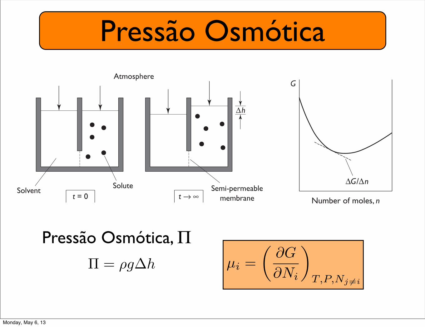
Osmosis is an equilibrium phenomenon that involves a semi-permeable membrane (not necessarily a biological membrane). Semi-permeable in this contextmeans that there are pores in themembranethat allow smallmolecules like solvents, salts, andmetabolites topassthrough but prevent the passage of macromolecules like DNA, poly-saccharides, andproteins. Biologicalmembranesare semi-permeable:large solute molecules are impermeant. Like freezing point depressionand boiling point elevation, osmosis is a colligative property.
Suppose we have an osmometer, also called a U-tube, with armsseparated by a semi-permeable membrane (Fig. 5.9). Let the tem-perature be constant. If no solute is present the height of the solventis the same on both sides, because the pressure of the externalenvironment is the same on both sides. The situation changes onintroduction of an impermeant solute to one side. Let the solute be alargish protein, say hemoglobin, and let it be freeze-dried beforebeing added to the solvent. Freeze-dried protein occupies a relativelysmall volume. Initially, the height of the fluid is the same on bothsides of the osmometer, just as when no solute was present. Butwhereas before the solute occupied a small volume on the bench-top,now it is able to move freely throughout one side of the osmometer.There has been a large increase in the entropy of the solute! (If you arenot surewhy, see the discussion onperfume inChapter 3.)We requirethat the solute particles be free to roam about the entire volume ontheir side of themembrane, but that they not be able pass through themembrane. And just as a confined gas pushes against the walls of itscontainer (Chapter 2), the solution pushes against the atmosphereand against thewalls of the osmometer.What happens? There is a nettransfer of solvent from the side where no solute is present to theother side. This decreases the volume of pure solvent and increasesthe volume of solution. How can we explain what has happened?
Addition of solute to solvent reduces the chemical potential ofthe solvent (Chapter 4). This creates a difference in the chemicalpotential of the solvent between the pure side and the impureside. The difference in chemical potential is thermodynamically
Fig. 5.9 A simple osmometer. A
solute can move freely in a fraction
of the total volume of solvent. The
solution is separated from pure
solvent by a membrane that is
permeable to the solvent but not
the solute. There is a net flow of
solvent from the pure solvent to the
solution, resulting in the
development of a head of pressure.
This pressure is the osmotic
pressure, !! "g1h, where " is
density of the solvent, g is
gravitational acceleration, and 1h is
the difference in fluid levels. As
described by van’t Hoff, !!CVoRT/m, where C is the mass of solute in
the volume of solvent, Vo is the
partial molar volume of the solvent,
and m is the molecular mass of the
membrane-impermeant solute.
Note that ! is an approximately
linear function of C under some
conditions. Osmotic pressure data
can thus be used to measure the
molecular mass of an osmotic
particle.
148 GIBBS FREE ENERGY – APPLICATIONS
Pressão Osmótica, Π⇧ = ⇢g�h µi =
✓@G
@Ni
◆
T,P,Nj 6=i
enough) and pressure (1 atm). The activity of a substance, a conceptintroduced by the American Gilbert Newton Lewis (1875–1946), is itsconcentration after correcting for non-ideal behavior, its effectiveconcentration, its tendency to function as a reactant in a given che-mical environment. There are many sources of non-ideality, animportant one being the ability of a substance to interact with itself.
Ideal behavior of solute A is approached only in the limit ofinfinite dilution. That is, as [A]! 0, !A! 1. In the simplest case, theactivity of substance A, aA, is defined as
aA ! !A"A#; $4:4%
where !A is the activity coefficient of A on the molarity scale. When adifferent concentration scale is used, say the molality scale, a dif-ferent activity coefficient is needed. The concept of activity is basi-cally the same in both cases. According to Eqn. (4.4), 0< aA< [A]because 0< !A<1. Activity is a dimensionless quantity; the units ofthe molar activity coefficient are l mol&1.
Defining 1G' at unit activity, while conceptually simple, is pro-blematic for the biochemist. This is because free energy changedepend on the concentrations of reactants and products, and theproducts and reactants are practically never maintained at molarconcentrations throughout a reaction! Moreover, most reactions ofinterest do not occur at standard temperature. Furthermore, bio-chemistry presents many cases where the solvent itself is part of areaction of interest. We need a way to take all these considerationsinto account when discussing free energy change.
The relationship between the concentration of a substance A andits free energy is defined as
„A & „'A ! RT ln aA; $4:5%
where !A is the partial molar free energy, or chemical potential, of A, and„'A is the standard state chemical potential of A. The partial molar
free energy of A is, in essence, just 1GA/1nA, or how the free energyof A changes when the number of molecules of A in the systemchanges by one (Fig. 4.8). The chemical potential of A is a function ofits chemical potential in the standard state and its concentration.Equation (4.5) could include a volume term and an electrical term(there are numerous other kinds of work, see Chapter 2), but let’sassume for the moment that the system does not expand against aconstant pressure and that no charged particles are moving in anelectric field. It is appropriate to call „ the chemical potentialbecause at constant T and p, G is a function of chemical compositionalone.
Equation (4.5) tells us that when aA! 1, „A & „'A ! 0. That is
„A & „'A measures the chemical potential of A relative to the stan-
dard state conditions; the activity of a substance is 1 in the standardstate. The chemical potential also depends on temperature asshown, and the gas constant puts things on a per-mole basis.Equation (4.5) also says that the chemical potential of a solvent
Fig. 4.8 Thermodynamic potential
and solute concentration. The
Gibbs free energy of a solute varies
with concentration. The chemical
potential measures the rate of
change of G with n, or the slope of
the curve at a given value of n (1G/1n). Note that G can decrease or
increase on increases in
concentration.
CHEMICAL POTENTIAL 99
Monday, May 6, 13

Pressão Osmótica
µi =
✓@G
@Ni
◆
T,P,Nj 6=i
�G = µ1�N1
A B11
11
1
1
1
1
1
1
�G = (µ1�N1)|A + (µ1�N1)|B= µ1 (�N1|A + �N1|B)
No equilíbrio:0 = µ1 (�N1|A + �N1|B)
�N1|A = � �N1|BMonday, May 6, 13
Pressão Osmótica
µi =
✓@G
@Ni
◆
T,P,Nj 6=i
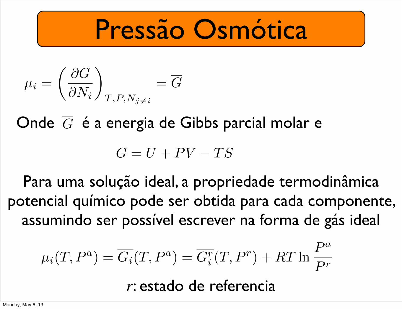
= G
Onde é a energia de Gibbs parcial molar eG
Para uma solução ideal, a propriedade termodinâmica potencial químico pode ser obtida para cada componente,
assumindo ser possível escrever na forma de gás ideal
µi(T, Pa) = Gi(T, P
a) = Gri (T, P
r) +RT lnP a
P r
G = U + PV � TS
r: estado de referenciaMonday, May 6, 13

Pressão Osmótica
2
AB
2
2
11
11
1
1
1
11
é o coeficiente de atividade do solvente
�1
⇧ = �RT
V
ln(�1x1)
x1 é a fração molar
O coeficiente de atividade quantifica o desvio que uma mistura de substâncias químicas faz em relação o
comportamento de uma mistura ideal. Numa mistura ideal, cada componente interage da mesma
forma (ΔH=0)
Monday, May 6, 13

Pressão Osmótica
Para concentrações baixas a equação de Morce pode ser utilizada:
⇧ = (iM)RT Pressão Osmótica
M é a molaridade e i é o fator de Van’t Hoff que é a razão entre a concentração atual de partículas produzida quando uma substância é diluída e a concentração da substância calculada por sua massa.
Para substâncias não eletrolíticas i=1
PV = nRT
P =n
VRT
P = MRT , M =n
V
Monday, May 6, 13

Pressão Osmótica
This is the van’t Hoff law of osmotic pressure for ideal dilute solu-tions, named in honor of the scientist who gave Pfeffer’s work amathematical foundation.8 Equation (5.11) can be used to measurethe mass of an impermeant solute particle (though there are easierand more accurate ways to do it). Note how Eqn. (5.11) looks likeEqn. (4.12). You may already have noticed how closely Eqn. (5.11)resembles the ideal gas law (pV! nRT or p! nRT/V!CRT, where n isnumber of particles and C is concentration). C2, the concentration ofsolute, is the mass of solute particles added to a known volume ofpure solvent. What van’t Hoff found was that the measured osmoticpressure was basically the pressure of n solute particles movingaround in volume V, the volume of the solvent through which thesolute particles are free to move!
The degree to which Eqn. (5.11) matches experimental resultsvaries with concentration and solute (Fig. 5.10). There are severaldifferent ways of trying to cope with the situation, but our concernwill be with just one of them here. Time is spent on it at all becauseit’s a generally useful method. We express the thermodynamicobservable quantity (here, !) as a series of increasing powers of anindependent variable, (here, C) and check that the dominant term isthe same as we found before (Eqn. (5.10)) when the independentvariable takes on an extreme value (low concentration limit, as weassumed above):
! ! C2RT
M2"1# B1"T$C2 # B2"T$C2
2 # . . .$: "5:12$
The Bi(T) terms are constant coefficients whose values are solute-and temperature-dependent and must be determined empirically. IfC2 is small, only the first term makes a significant contribution to !
(convince yourself of this!), just as in Eqn. (5.10). If only the first two
Fig. 5.10 Osmotic pressure
measurements. Osmotic pressure
increases with concentration of
solute, as predicted by the van’t
Hoff law. The pressure at a given
concentration of solute depends
significantly on the solute. If the
solute is a salt, dissociation in
aqueous solution will result in a
greater number of particles than
calculated from the molecular mass
of the salt. The van’t Hoff law is
exact for an ideal solution. At high
solute concentrations, non-linear
behavior can be detected. Such
behavior can be accounted for by
higher order terms in C. The data
are from Table 6–5 of Peusner
(1974).
8 The Dutch physical chemist Jacobus Henricus van’t Hoff (1852–1911) was therecipient of the Nobel Prize in Chemistry in 1901, the first year in which theprestigious awards were made.
OSMOSIS 151
Monday, May 6, 13

Dialise
ratio and relative abundance of these will have an impact on themigration of water through the membrane.
And equilibrium dialysis? In some respects it’s rather similar tonon-equilibrium dialysis. In others, it has a more specific meaningthan dialysis and therefore deserves to be treated somewhat sepa-rately. Suppose you are interested in the binding of a macro-molecule to a membrane-permeant ligand. This presents anopportunity for quantitative analysis of the binding interaction. Tosee how, suppose we have a two-chambered device like that shownin Fig. 5.12. In the left side, you introduce a known amount ofmacromolecule in your favorite buffer, and on the right side, aknown amount of ligand dissolved in the same buffer. The ligandwill diffuse in solution, and the net effect will be movement downits concentration gradient, through the membrane. By mass actionthe ligand will bind to the macromolecule. After a sufficiently longtime, the two chambers will be at equilibrium; the concentration offree ligand will be the same on both sides of the membrane. Theamount of ligand on the side of the macromolecule, however, willbe higher by an amount depending on the strength of interactionbetween macromolecule and ligand. You can then use a suitableassay to measure the amount of ligand on both sides of the mem-brane, and the difference will be the amount bound to the macro-molecule. You then compare the concentration of “bound” ligand tothe concentration of macromolecule and to the concentration of“free” ligand, and use the results to calculate the binding constantand the number of ligand molecules bound per macromolecule. Thisis an important topic. See Chapter 7.
Fig. 5.12 Equilibrium dialysis. At
the beginning of the experiment
(t! 0), the membrane-impermeant
macromolecule and membrane-
permeant ligand are on opposite
sides of a semi-permeable dialysis
membrane. The two-chambered
system is not at equilibrium. After a
long time (t!1), the concentration
of free ligand is approximately the
same on both sides of the
membrane, in accordance with the
Second Law of Thermodynamics.
The number of ligand molecules is
not the same on both sides of the
membrane, however, as some
ligands are bound to the membrane-
impermeant macromolecules. The
bound ligand molecules are
nevertheless in equilibrium with the
free ones. Measurement of the
concentration of free ligand at
equilibrium and the total
concentration of ligand determines
the amount of bound ligand at
equilibrium.
156 GIBBS FREE ENERGY – APPLICATIONS
Monday, May 6, 13