fitch residential mortgage-backed securities criteria

Fitch Residential Mortgage-Backed Securities CriteriaMark Douglass Rui Pereira Roeluf Slump(212) 908-0229 (212) 908-0766 (212) [email protected] [email protected] [email protected]

Origination and Servicing ReviewM. Diane Pendley(212) [email protected]

SummaryFitch IBCA introduces enhanced criteria for analyzingcredit risk in securities backed by pools of ‘A’ qualityresidential mortgages. This enhancement representsthe third generation of residential mortgage-backedsecurities (RMBS) criteria development since 1989. Ineach generation, Fitch IBCA has produced RMBS ana-

lytics that reflect changes in the mortgage industry andstate-of-the-art mortgage pool risk assessment.Fitch IBCA’s three major enhancements to the RMBSmodel are:➢ Fitch IBCA’s frequency of foreclosure (FOF) meth-

odology fully integrates data on the borrower’scredit profile with loan attribute data. For the firsttime, investors can obtain a detailed understandingof how borrower credit, as measured by credit bu-reau scores, together with loan variables such asloan-to-value ratio (LTV), can be used to determinemortgage default probabilities.

➢ Fitch IBCA’s loss severity model has been enhancedto include long-term regional home price trends.The home price trend enables Fitch IBCA to proac-tively identify regions where homes are overvaluedrelative to long-term trends and adjust market valuedecline scenarios appropriately. Conversely, regionswhere property values have declined substantiallybelow long-term trends will not be subject to undueadditional stress.

➢ Credit enhancement at each rating level is deter-mined using historical data on regional default ratesto project possible lifetime pool default scenarios.These projections reflect stress assumptions rang-ing from an expected case economic environmentthrough a severe national depression scenario. Inparticular, Fitch IBCA has identified the SouthernCalifornia experience of the 1990s as the best proxyfor a national ‘AA’ scenario given the severity of the

Structured Finance

Residential Mortgage Special Report

December 16, 1998

Inside Page

Frequency of Foreclosure Model . . . . . . . . . 2

Frequency of Foreclosure Rating Multiples . . . . 5

Market Value and Loss Severity Model . . . . . . 7

Other Loan Risks . . . . . . . . . . . . . . . . . 10

Other Risks . . . . . . . . . . . . . . . . . . . . 12

Loan Level Credit Enhancement . . . . . . . . . 13

AppendixA Model Development and Validation Performance Samples. . . . . . . . . . . . . . . . . . . 15B Modeling and Data Sources . . . . . . . . . . . . . . . 16C Regional FOF Multipliers . . . . . . . . . . . . . 17–18D ‘AAA’ Base Frequency of Foreclosure . . . . . . 18E Whatever Happened to Texas? . . . . . . . . . . . . 19F Regional Home Price Levels Relative to Equilibrium Trends. . . . . . . . . . . . . . . . . . . . . . . 20G How Expected Loss Coverage Is Calculated . . . . 21H Regional Classification Index and Map . . . . 22–23

www.fitchratings.com

downturn and the extensive supplyof relevant nonconforming ‘A’ qual-ity mortgage performance data.

These enhancements provide FitchIBCA with a modeling tool that ishighly sensitive to variations in risk lev-els of mortgage pools. This report de-tails the research supporting the modelrevisions as well as existing elements ofthe RMBS rating criteria, focusing oncollateral credit risk analysis.

Frequency of ForeclosureModel

Fitch IBCA’s FOF model has evolvedover time as more performance data hasbecome available and mortgage origina-tion practices have further developed.Fitch IBCA’s original investment-gradecriteria was based on a study of the per-formance of Federal Housing Agency(FHA) mortgages during the severeTexas recession of the 1980s. In thatstudy, Fitch IBCA determined that theborrower’s equity in the home, as evi-denced by the LTV, was the most sig-nificant indicator of mortgage defaultrisk. Borrowers with more equity wereshown to be less likely to default thanthose with less equity. This result isconsistent with the equity theory ofmortgage defaults, which holds that aborrower’s incentive to avoid foreclo-

sure is related to the perceived equityposition in the home.

In 1993, Fitch IBCA introduced specu-lative-grade criteria that incorporatedregional econometric forecasting of fore-closure rates and home prices based onlocal economic conditions, includingemployment and income, among otherthings. The criteria were further en-hanced in 1995 by expanding from 43to 75 regions and incorporating delin-quency data from Mortgage Informa-tion Corp. and home price data fromCase Shiller Weiss, Inc. Fitch IBCA’sregional foreclosure stress scenarios ex-tended the ability of the equity-basedmodel to address the effect of realistic

economic stresses on borrowers’ abilityto make monthly mortgage payments.

In early 1997, Fitch IBCA began adjust-ing equity-based default expectationsto reflect borrower credit information asit became regularly available in theform of Fair, Isaac & Co., Inc. (FICOSM)credit bureau scores. Credit scores havebeen widely used for many years inconsumer debt underwriting, and re-search conducted by a number of mort-gage market participants over the pastfew years have identified borrowercredit report information as a highlysignificant factor in predicting mort-gage defaults. Credit reports are pro-duced by the three major creditbureaus: Equifax, TransUnion, and Ex-perian. Credit reports provide informa-tion on the status of credit accounts ofconsumers, including pay history, utili-zation, number, type, and age of ac-counts. In addition to raw credit data,credit bureaus also generate creditscores, most commonly FICO scores(see box above left), which are similarlyavailable from all three repositories.The evidence of FICO scores’ correla-tion to mortgage credit risk shows thatthe same credit report attributes thatindicate relatively higher consumercredit default risk also indicate highermortgage default risk, although mort-gage defaults will be much lower on anabsolute basis due to borrower popula-

Fair, Isaac & Co., Inc. Credit Bureau Score SummaryPerformance Criterion: Relative likelihood of more than 90 day delin-quency on any tradeline over the next 24 months

Risk Variables Categories: Previous credit performance, including: pres-ence of major derogatories — foreclosures, judgments, liens, bankruptcies,collections and chargeoffs, and payment history for revolving and installmentdebt (prevalence, recency and severity of delinquency); current level ofindebtedness; type of accounts (e.g. bank or finance company); number ofaccounts; pursuit of new credit; length of credit history (time)

Data Sources: Entire consumer credit databases at the three nationalcredit repositories (Equifax, Experian, and TransUnion)

Brands: BEACONSM, Experian/Fair, Isaac, and EMPIRICA®

Scale: 375–900 (approximately) logarithmic; lower scores indicate higher risk

Default DefinitionThroughout this report, the terms default rate and frequency of foreclo-sure are used interchangeably. Technically speaking, defaults do notalways result in foreclosures, foreclosures do not always result in losses,and losses are not always a result of foreclosures. Fitch IBCA’s analysisincluded measuring alternative definitions of default, including morethan 90 days delinquent, foreclosure initiation, real estate owned (REO)status, and other intermediate measures. Fitch IBCA found the morethan 90 days delinquent performance measure to be most useful for ratingassumptions in terms of predicting the borrower’s likelihood of perform-ing. Other definitions, such as foreclosure or REO, are influenced byservicing and loss mitigation practices and other circumstances likelyunknown at the time of origination or securitization.

Fitch Residential Mortgage-Backed Securities Criteria

2 Fitch, Inc.

tion and underwriting differences, andborrowers’ natural default priorities, in-cluding foreclosure disincentive.

The use of credit scores in mortgageunderwriting has become widespreadover the past few years, largely due tothe endorsement of credit scores as anunderwriting tool by the Federal HomeLoan Mortgage Corp. (Freddie Mac)and Federal National Mortgage Asso-ciation (Fannie Mae) in 1995. By 1997,most major mortgage originators were ob-taining credit score information and incor-porating it into lending decisions andprocesses, particularly through the use ofminimum FICO score requirements.This criteria revision formally integratescredit-score and loan-to-value risk driversinto a new multivariate risk assessmentframework based on historical performanceanalysis of nonconforming mortgages.

The most significant challenge in ana-lyzing the application of credit scores tomortgages is the lack of historical data.Since FICO has been widely capturedby mortgage lenders only in the pastfew years, there is not a ready supply ofseasoned loan pools with statisticallysignificant default rates and associatedorigination FICO scores. Fitch IBCAaddressed this challenge through theuse of retro scoring. Retro scoring is aservice offered by the credit bureauswhereby archival data regarding a bor-

rower’s credit at some point in the pastis retrieved and a credit score is gener-ated based on that data. By obtainingretro scores for seasoned pools of mort-gages at or near the time the mortgageswere originated, a statistically valid per-formance sample was created. For de-tails on the default model sample, seeAppendix A, page 15.

Fitch IBCA conducted an extensivemultivariate regression analysis of thesample data. Also, Fitch IBCA con-sulted with many industry leaders inthe application of credit-scoring tech-nology to mortgage lending. The resultof this analysis is an FOF model thatsets a new standard for credit ratinganalysis. The power of the new model

‘CCC‘ Base Frequency of Foreclosure — 30-Year Fixed-Rate Mortgages(%)

–––––––––––––––––––––––––––––––––––––––––––––––––––––– FICO Score –––––––––––––––––––––––––––––––––––––––––––––––––LTV 580 600 620 640 660 680 700 720 740 760 780 800 820

60 1.6 1.2 0.9 0.7 0.5 0.4 0.4 0.3 0.3 0.3 0.2 0.2 0.265 2.3 1.6 1.2 0.9 0.7 0.5 0.4 0.4 0.3 0.3 0.3 0.2 0.270 3.3 2.3 1.7 1.2 0.9 0.7 0.5 0.4 0.4 0.3 0.3 0.3 0.275 4.8 3.4 2.4 1.7 1.2 0.9 0.7 0.6 0.5 0.4 0.3 0.3 0.380 6.9 4.9 3.4 2.4 1.7 1.2 0.9 0.7 0.6 0.5 0.4 0.3 0.385 9.7 7.0 5.0 3.5 2.5 1.8 1.3 0.9 0.7 0.6 0.5 0.4 0.390 13.2 9.9 7.2 5.1 3.6 2.5 1.8 1.3 1.0 0.7 0.6 0.5 0.495 17.4 13.4 10.0 7.3 5.2 3.7 2.6 1.8 1.3 1.0 0.7 0.6 0.5100 22.1 17.7 13.6 10.2 7.4 5.3 3.7 2.6 1.9 1.3 1.0 0.7 0.6

Assumes full documentation, purchase, primary occupancy, single-family detached, and $300,000 initial balance. LTV – Loan-to-value ratio.FICO – Fair, Isaac & Co., Inc.


Fitch, Inc. 3

is illustrated in the chart at the toppage 3. This chart depicts the risk rank-ing of loans by three models as meas-ured by an “ever over 90 daysdelinquent” performance criterion (seeDefault Definition box, page 2). Eachgroup of bars represents a decile of thedistribution of loan risk as assessed byeach model. Each bar in a group indi-cates the percentage of the defaultedloans in the sample that each modelranked as belonging in that decile. Theefficiency of a model can be seen inhow well it places defaulted loans in thehigh-risk deciles. The bars labeled“Equity Model” depict the risk rank-ing of loans using Fitch IBCA’s equity-based investment-grade model withoutany credit-scoring adjustments. Thebars labeled “FICO Alone” show therisk ranking of loans if only the FICOscore is considered. The bars labeled“Fitch IBCA Model” indicate the riskranking using Fitch IBCA’s new meth-odology. The pool used for this chart isa validation sample, not the develop-ment sample. That is, the results reflectthe application of the model to loansthat were not used to develop themodel.

The chart at the top of page 3 illustratesthat FICO scores are more effective atdistinguishing between defaulted andnondefaulted loans than the equity-based model. Moreover, the chartshows that Fitch IBCA’s enhancedmodel is more predictive than either ofthe component variables. This can beseen in the degree to which those loansindicated as highest risk by the FitchIBCA model had the highest percent-age of defaulted loans. Also, those loansdetermined to be less risky by FitchIBCA’s model have a lower incidence ofdefault. Most strikingly, the progressionof default rates from highest risk bucketto lowest risk is very smooth, stronglysuggesting that the major risk factorshave been accounted for.

The table at the bottom of page 3 showsFitch IBCA’s base case (equivalent to a

‘CCC’ rating level) lifetime FOF ex-pectations for 30-year fixed-rate mort-gages. Each entry in the table representsthe probability of default assigned to aloan based on the LTV and FICO score(note that the table entries representpoints along a continuous distributionof probabilities). Base case prob-abilities reflect the likelihood of de-fault without the addition of stressfactors related to economic downturns.In examining the table, it is importantto note the spread in FOF expectationsfrom the lowest to highest risk loans.Loans with very low LTVs and veryhigh FICO scores enjoy FOF expecta-tions as low as 0.2%. Loans with very

high LTVs and borrower FICO scoresbelow 600 are assigned FOFs of morethan one hundred times greater. Per-formance data indicate that the FICOscore is a more significant factor thanLTV, and this is reflected in FitchIBCA’s FOF expectations. The sensi-tivity of the Fitch IBCA model tochanges in each variable makes for amodel that will pick up subtle vari-ations in pool quality to an unprece-dented degree.

Regional Adjustments to FOFExpectationsSince 1993, Fitch IBCA’s mortgage de-fault criteria has incorporated regional

Bond Default Rates and FOF Stress MultiplesAltman

StudyAltman

Study Excess Implied1971–1991 1971–1995 Foreclosure Mortgage Pool Multiple

Rating Default (%)* Default (%)** Probability (%) Default (%) of ‘CCC’ FOF

‘AAA’ 0.2 0.1 0.1 15.1 9.9‘AA’ 1.9 0.9 0.5 11.6 7.6‘A’ 1.5 0.9 1.0 10.0 6.6‘BBB’ 4.8 3.8 3.0 7.7 5.0‘BB’ 16.3 19.5 15.0 4.1 2.7‘B’ 37.9 35.5 37.5 2.1 1.4‘CCC’ 38.9 58.3 50.0 1.5 1.0

*Edward Altman, “Revisiting the High-Yield Bond Market” (Summer 1992), page 86. **EdwardAltman and Vellore Kishore, “Defaults and Returns on High Yield Bonds: Analysis Through 1995”(January 1996) exhibit 10. FOF – Frequency of foreclosure.


4 Fitch, Inc.

foreclosure forecasts developed byWEFA (see Appendix B, page 16). WEFA’sforecast regional foreclosure rate is afunction of delinquencies, home prices,housing starts and home sales, employ-ment, population, and demographics.Regional variations in delinquency andforeclosure rates continue to play an im-portant role in the determination of fore-closure frequency. In the enhancedFitch IBCA model, the base case FOFdetermined for each loan as a functionof LTV and FICO score is adjusted bya multiplier that reflects the differencebetween WEFA’s national average fore-cast of foreclosure rates and WEFA’sforecast for the region in which the loanmortgaged property is located in. Ap-pendix C pages 17 and 18 shows theregional multipliers for the 75 regionsFitch IBCA tracks at each rating level.In the ‘CCC’ expected case, WEFA’sforeclosure rate forecast for the Min-neapolis-St. Paul, MN region is ap-proximately one-half that for the nationas a whole. Base case expectations forBaltimore, MD are close to the nationalaverage, while those for Los AngelesCounty, CA are more than twice ashigh. These multipliers converge on1.0 at the ‘AAA’ level. This conver-gence reflects Fitch IBCA’s approach toincorporating regional default expecta-tions across the rating spectrum. At thespeculative-grade and low investment-grade rating levels, realistic expecta-tions regarding individual regions areimportant considerations. Conversely,at the ‘AA’ and ‘AAA’ levels, the modelsimulates a severe national depression.At these levels regional variations be-come much less significant while themultiples of default expectation associ-ated with the stress scenario becomemuch more significant.

Frequency of ForeclosureRating Multiples

Regional Stress AnalysisRating multiples of foreclosure fre-quencies in Fitch IBCA’s enhanced cri-teria are based on analysis of regional

foreclosure rates. The Regional Distri-bution of Mortgage Default Rates chartat the top of page 4 shows the distribu-tion of regional foreclosure rates acrossthe 75 regions tracked by Fitch IBCA,together with a trend line. Each bar onthe chart represents the cumulativeforeclosure rate over several years forone region. Rating multiples are deter-mined by selecting points along thedistribution curve. To determine theappropriate points on the distributioncurve to associate with each ratinglevel, Fitch IBCA looked to data ondistributions of bond default rates. The

first two columns of the Bond DefaultRates and FOF Stress Multiples tableat the bottom of page 4 shows the re-sults of two studies by Edward Altmanof corporate bond default rates. TheAltman studies indicate the percentageof bonds at each rating class that havedefaulted and are useful in under-standing the relative risk of ratings.Fitch IBCA has used this data to deter-mine the relative multiples of FOF ex-pectations to associate with each ratinglevel. The third column of the table,“Excess Foreclosure Probability,” showsFitch IBCA’s expectation of the likeli-


Fitch, Inc. 5

hood of excess foreclosures, that is thelikelihood that a pool’s lifetime FOFwill exceed the FOF level assigned fora given rating. As the table shows, only0.1% of pools should experience fore-closures exceeding Fitch IBCA’s ‘AAA’FOF stress, while FOFs can be ex-pected to exceed the ‘CCC’ level 50%of the time. Column 4, “Implied Mort-gage Pool Default Percentage,” showsthe lifetime expectation for each ratinglevel for the historical sample. TheseFOFs are determined by selecting thepoints on the distribution curve of re-gional results that correspond to thedesired probabilities of excess foreclo-sures. For example, since the CCCprobability of excess foreclosures is50%, the corresponding point on theregional result distribution is the mid-point. Therefore, 50% of the regionalFOF outcomes will be less than the’CCC’ FOF expectation, while 50%will be greater. The midpoint of thetrend line indicates a projected lifetimeFOF of approximately 1.5%, so the ex-pected ‘CCC’ FOF is set to 1.5%. Notethat these default frequencies arebased on the regional results after ad-justing to a projected lifetime FOF. Ac-

tual pool frequencies will vary as a func-tion of the distribution of expected de-fault rates for a given pool. The lastcolumn of the table shows the FOFrating multiple relative to ‘CCC’.

Using this methodology, the ’AA’ fore-closure frequency expectation is roughly

equivalent to the historical Los Angelesexperience, while the ‘CCC’ base casecorresponds to the Washington, D.C. ex-perience. The “Unemployment Rates”and “Foreclosure Rates” charts on page 5illustrate the relative economic experi-ences in these regions. The first chartshows the unemployment rate in thesetwo regions, together with the U.S. rate.While Washington, D.C. and the U.S. asa whole experienced a short, sharp reces-sion in the early 1990s, this chart illus-trates that the Los Angeles regionexperienced a much deeper and moreprolonged recession. The second chartdepicts the foreclosure rates for theseregions during the same time period.Changes in foreclosure rates in theseregions closely tracked the changes inunemployment rates, again showing amuch more severe problem for Los An-geles. (For a comparison of the Los Angelesexperience to the 1980s Texas recession dataused to develop the original default model,see the “Whatever Happened to Texas” box,Appendix E, page 19.)

Frequency of ForeclosureMultiples Vary by Loan RiskIn reviewing historical foreclosure fre-quency data, Fitch IBCA observed that


6 Fitch, Inc.

the relative response to external stressvaried among loans as a function of loanrisk. Loans with low risk in the basecase had a higher default multiple un-der stress than high-risk loans. This isillustrated in the chart at the top ofpage 6, which shows the relative de-fault rate for loans with similar risk indifferent regions. This chart indicatesthat low-risk loans have much higherrelative default rates under stress thanhigh-risk loans. This is not surprisinggiven that low-risk loans have such alow absolute foreclosure frequency ex-pectation that an external stress, suchas a sharp rise in unemployment, canhave a large relative effect. Conversely,high-risk loans have such a large basecase default expectation that stressmultiples cannot be very large or fore-closure frequencies in excess of 100%would be implied.

Using the analysis of relative defaultrates based on loan risk, Fitch IBCAassigns rating multiples as a function ofbase case foreclosure frequency. Thechart at the bottom of page 6 shows theFOF multiples for each rating level forloans in each risk bucket. The tableabove right shows FOFs and rating multi-ples for various loan risk examples.

Fitch IBCA’s methodology for calculat-ing foreclosure frequency rating multiplesprovides for a dynamic response to vari-ations in pool risk characteristics within aframework of historical stress analysis. Ap-pendix D on page 18 shows ‘AAA’ FOFsresulting from this methodology for vari-ous FICO/LTV combinations.

Market Value and LossSeverity Model

Fitch IBCA’s Regional Approachto Market ValueFitch IBCA utilizes a regional approachto developing home price trends andmarket value stress scenarios. In addi-tion to the mortgage foreclosure rateprojections described earlier, FitchIBCA, working with WEFA, developed

a system of econometric models thatare used to forecast single-family homeprices. Through regression analysis ofregional economic conditions (e.g. un-

employment and housing starts, amongothers) combined with historical homeprice data, WEFA generates homeprice forecasts together with six stress

FOF Rating Multiple ExamplesEach loan is assumed to be a $300,000, 30-year fixed-rate, full documentation, single-family detached, primary residence purchase financing.

Credit Quality Low Risk Moderate Risk High Risk

FICO Score 780 700 600LTV (%) 60 80 95‘AAA‘ FOF (%) 3.34 9.21 73.56‘AA’ FOF (%) 2.51 7.05 58.41‘A’ FOF (%) 2.14 6.15 53.11‘BBB’ FOF (%) 1.53 4.64 44.74‘BB’ FOF (%) 0.80 2.54 26.56‘B’ FOF (%) 0.37 1.32 17.71‘CCC’ FOF (%) 0.24 0.91 13.25

Rating ––––––––– Stress Multiple (Relative to ‘CCC’) ––––––‘AAA’ 13.63 10.15 5.55‘AA’ 10.24 7.77 4.41‘A’ 8.76 6.77 4.01‘BBB’ 6.26 5.11 3.38‘BB’ 3.28 2.79 2.00‘B’ 1.52 1.46 1.34‘CCC’ 1.00 1.00 1.00

FOF – Frequency of foreclosure. *FICO – Fair, Isaac & Co., Inc. LTV – Loan-to-value ratio.


Fitch, Inc. 7

scenarios for each of the 75 regionsFitch IBCA tracks (see Appendix H,pages 22 and 23).

The recessionary scenarios reflect in-creasingly severe assumptions appliedto the forecasts for the economic vari-ables affecting home prices. The sce-narios are calibrated across regions bycalculating the standard deviation fromthe trend for each economic variableover the past two decades and usingthese ranges to determine the severityof economic stress assumptions appliedto the exogenous variables over the sixstress scenario projections. Each sce-nario represents a cycle of economicshock, recession maintenance, and re-covery. The forecast and stress scenariodata are updated semiannually. Thechart at the bottom of page 7 is anexample of a regional home price fore-cast, together with stress scenarios forthe Santa Barbara County, CA region.The table above defines the relation-ship between standard deviation sce-narios and rating categories.

Introduction of EquilibriumHome Price TrendFitch IBCA has enhanced the homeprice model by introducing a long-termhome price equilibrium trend into theregional home price forecasts. The dra-matic rise of home prices in SouthernCalifornia in the late 1980s and the en-suing decline through the 1990–1996period highlighted the need for a homeprice model that could identify bothspeculative bubbles and relative de-pression in regional real estate markets.

In enhancing the regional models toidentify such market conditions, FitchIBCA, working with WEFA, startedwith the theory that, even in an effi-cient market, prices at any point in timecould reflect irrational optimism or pes-simism but, over the long run, wouldtend to approach an equilibrium levelor trend. Trial models were built usingseveral different variables, includingsmoothed national home prices, per-sonal income, employment, and house-holds by age. Many of these variableshad similar cycles that coincided withthe home price run-up around 1990. Asa result, they actually fit the data toowell, explaining up to 90% of the local

home price variation. These measureswould produce a model that tracks theactual local home price but provides noinsights into identifying pricing bubbles.

The solution to this problem is a modelthat estimates housing affordability.Using this model, Fitch IBCA forecastsan equilibrium trend of home pricegrowth for each region. Regions wherehome prices outrun affordability can beexpected to eventually correct to thelevel indicated by the long-term trend.Conversely, regions where home pricesappear low relative to the trend can beexpected to recover over time.

Fitch IBCA constructed a proxy for na-tional affordability by assuming an av-erage income household, with a 28%mortgage-to-income ratio at prevailingmortgage rates and then computing thevalue of a house that could be pur-chased at 80% LTV. Applying this cal-culation indicates that there was anational home price bubble around1990, since affordability weakens in thelate 1980s and recovers only gradually

Market Value Decline ScenariosRating Economic Driver/Scenario

‘CCC’ Baseline Forecast‘B’ 0.5 Standard Deviation‘BB’ 1.0 Standard Deviation‘BBB’ 2.0 Standard Deviations‘A’ 3.0 Standard Deviations‘AA’ Average Value of ‘AAA’ and ‘A’ Scenarios‘AAA’ 6.0 Standard Deviations


8 Fitch, Inc.

until 1992. This result matches ob-served home price behavior, particu-larly for the upper tier markets locatedon the coasts.

The regional home price equilibriumtrends (EQTs) are determined by re-gressing each region’s home prices onnational affordability and also takinginto account the local share of high-in-come (more than $100,000 per year)households. Concentrations of high-in-come households in a region will alterthe definition of “affordability” for thatregion. The home price forecast for a re-gion now draws on local economic condi-tions (unemployment rates, home salesand housing starts, income, total em-ployment, and demographic composi-tion) as well as the relationship betweenrecent local home prices and the EQT.The influence of the EQT on the fore-cast increases as the spread between re-cent prices and the trend price levelgrows, thus exerting more “pull” on theforecast back toward the long-term trend.

The charts on pages 8 and 9 illustratethe effect of the equilibrium trend. The

chart at the bottom of page 8 shows theEQT and home price forecast alongwith each rating stress scenario for thePhoenix, AZ region. The chart above

contains the same information for theLos Angeles region. Phoenix is a regionwhere home prices have recently ex-ceeded the equilibrium trend, whereasLos Angeles is only now emerging fromsignificant home price deflation. Theimpact of these factors on both thehome price forecast for each region aswell as the stress scenarios is shown inthese charts. In the Phoenix region, theEQT forces the home price forecast toa steady-state that eventually con-verges on the trend line. Also, the stressscenarios indicate substantial early de-clines as prices correct significantly. Inthe Los Angeles region, forecast homeprices rise through the trend line, andstress scenario declines are muted bythe long-term reversion to the trend.

The development of regional EQTsprovides Fitch IBCA with a uniqueability to prospectively account forvaluation booms and busts. Appen-dix F on page 20 ranks the spread be-tween current home prices and theEQT for the 75 regions.


Fitch, Inc. 9

Market Value Decline RatingMultiplesFitch IBCA’s market value declinemodel is consistent with the foreclo-sure frequency model in its identifica-tion of the Los Angeles experience ofthe early 1990s as the benchmark for‘AA’ expectations. The chart at the bot-tom of page 9 compares the historicalhome price decline experienced in LosAngeles together with Fitch IBCA’sprojections for Salt Lake City, UT. Inthe run up to the Olympic Games of2000, Salt Lake City is exhibiting thesort of overheating in the home pricemarket that Los Angeles experienced.The chart shows that the ‘AA’ expecta-tion for Salt Lake City most closely ap-

proximates the Los Angeles experi-ence. The table at left shows the sever-ity of market value decline for each ratinglevel for the Salt Lake City region.

FOF and MVD ProjectionsThe Fitch IBCA RMBS model projectsboth frequency of foreclosure and mar-ket value decline scenarios over timingcurves consisting of 56 quarters (14years) as shown in the chart below. Theforeclosure frequency curve is not aloan seasoning curve but rather reflectsthe impact of the rating stress scenario.Both the FOF curve and the MVDcurve assume the immediate onset ofthe stress scenario with peak stress oc-curring in the tenth quarter and thenslowly ramping back down to base caselevels over several years. Fitch IBCAbelieves that the synchronization of theFOF and MVD curves is a conservativemethodology that reflects the historicalcoincidence and interrelation of sharphome price declines and foreclosure ratespikes. The chart also shows the loss se-verity resulting from the interaction of theMVD scenarios with the other elements ofthe loss severity calculation. For a detaileddiscussion of the loss coverage calcula-tion, see Appendix G on page 21.

Other Loan RisksFitch IBCA adjusts the foreclosurerates and market value expectations ona loan-by-loan basis to account for indi-vidual loan characteristics of the collat-eral. Foreclosure rates are adjusted forreduced-documentation programs,cash-out refinances and non-owner-oc-cupied properties. Market value is ad-justed for non-single-family propertiesand high value properties.

Foreclosure Rate Adjustments

15-Year, ARM, and Other Products:Performance data results, as well assubstantial MBS static pool experience,affirm 15-year, fixed-rate loans’ supe-rior performance to the standard 30-year product and reveal attributes thatwould lead one to expect such perform-ance in terms of higher FICO score dis-tributions and lower original LTVdistributions. Fitch IBCA believes that thevoluntary undertaking of a substantiallyincreased payment obligation represents apremium borrower selection mechanism,whereas adjustable-rate mortgages(ARMs) and other lower payment alter-natives represent potential adverse se-lection mechanisms, particularly ifcombined with flexible underwritingstandards. Some ARM performance insecuritized pools has been poor and re-flects such risk layering.

Sourcing and potential adverse pool se-lection will be a key concern of FitchIBCA in evaluating ARM and otherpool submissions and it, along with thedegree of coupon discount (i.e. adverseborrower selection), will change ourARM FOF premiums relative to fixed-rate products.

Reduced Documentation Programs:Analysis of the model developmentsample reveals that loans made withreduced documentation are more likelyto default than fully documented loans.Loans made with no borrower incomeverification and no asset verification re-quired are much more likely to defaultthan full documentation loans. Loans

Market Value Declines forSalt Lake City, UT(Weighted Average Over FOF Stress Curve)

(%)

‘AAA’ 48.80‘AA’ 42.31‘A’ 35.83‘BBB’ 31.10‘BB’ 26.75‘B’ 25.22‘CCC’ 21.37

FOF – Frequency of foreclosure.


10 Fitch, Inc.

with little or no documentation performparticularly poorly when combined withother high-risk characteristics, such aslow credit scores and high LTVs. Forloans without income verification, FOFsmay be increased as much as 300%,depending on the mix of other risk fac-tors. No-documentation loan FOFsmay be increased as much as 500%.

When evaluating limited documenta-tion programs, Fitch IBCA reviews pro-gram guidelines and discusses theprogram’s features and historical per-formance with management. Issuers,particularly those originating ‘alterna-tive A’ loans, often develop specific un-derwriting criteria designed to mitigatethe risk associated with limited docu-mentation. Fitch IBCA considers thesemitigating factors and associated per-formance data in assigning credit en-hancement levels.

Cash-Out Refinancing: Homeownersrefinance to take equity or cash out oftheir homes based on either increasedproperty value or the availability ofhigher LTV loans. Borrowers today canrefinance 100% or more of their prop-erty’s value. Loan performance data in-dicate that cash-out refinancings aremore likely to default than rate andterm refinancings. First, given the bor-rowers incentive to obtain a desiredamount of cash, pressure to reach thecorresponding property valuation mayresult in understated LTVs. Therefore,such loans would be more risky thanaccurately valued loans with apparentlyidentical LTVs. Review of appraisalprocesses helps Fitch IBCA to gaugethis risk in rated pools. Second, a com-mon purpose for cash-out refinancing isdebt consolidation. While debt consoli-dation may result in a lower aggregatemonthly payment for the borrower, theneed for debt consolidation can be anindicator of financial stress. Should theborrower “reload” on other credit linesafter the consolidation, the debt burdenmay become intolerable. Fitch IBCA ad-

justs cash-out loan default frequenciesupward by as much as 300%.

Second Home and Investor Proper-ties: Loan performance data supportsthe assumption that borrowers thathave mortgaged their primary resi-dence have a greater disincentive todefault than those borrowing againstsecond homes and investment proper-ties. Fitch IBCA increases the foreclo-sure rate on second homes by as muchas 25% and on investment propertiesby as much as 100%.

Multifamily Homes/Attached Homes:Single-family detached homes exhibitthe best foreclosure performance amongproperty types. Fitch IBCA adjusts fore-closure rates for multifamily properties byas much as 150% and adjusts condomin-ium FOFs by as much as 220%.

Loan Balance: Very large loans exhibithigher rates of default in the sampledata. Foreclosure frequency adjust-ments are made as balances increase.Consideration is given to the fact thatfor certain regions, large balances aremuch more common.

Mortgage Scoring Systems: Fitch IBCAfrequently receives pool data contain-ing mortgage score information. Pro-prietary mortgage scoring systemsdeveloped by mortgage insurers, origi-nators, and others are similar in conceptto credit bureau scores but are designedto specifically predict the likelihood ofmortgage default. Mortgage scoringsystems consider such factors as LTV,loan documentation level, borrowertime in the home, borrower time in thefield of occupation, and debt-to-in-come ratios, among other factors notconsidered in bureau scores. As a result,these systems offer demonstrablyhigher accuracy in separating good andbad loans than bureau scores alone.

Fitch IBCA has analyzed the effective-ness of mortgage scoring systems fromCiticorp Mortgage, GE Capital Mortgage

Insurance, Mortgage Guaranty Insurance,Norwest Mortgage, PMI Mortgage In-surance, and United Guaranty ResidentialInsurance and adjusts foreclosure fre-quencies to reflect the scoring system’sindicated loan risk. These adjustmentshave generally taken the form of adjust-ments to the equity-based FOFs, similarto the FICO score adjustments but lesserin degree to mitigate the potential forintroducing redundancy to the analysis.In light of the latest research and criteriarevisions, Fitch IBCA will be updating itsapproach to using mortgage scores in itsanalysis.

Seasoned Loans: Fitch IBCA considersseveral factors in the analysis of seasonedloans. Most important is information onloan performance. Fitch IBCA will re-duce foreclosure frequencies for loansthat have demonstrated good perform-ance over long periods and will alsoraise foreclosure frequencies for loansthat have been delinquent. In addition,FOFs for loans seasoned more than twoyears rely on an updated current LTVthat reflects recent home price changesand loan payments. Updated creditscore information will also be used whenavailable.

In analyzing seasoned pools, FitchIBCA reviews the prepayment historyof the pool to determine whether ad-verse selection has occurred. If the re-maining borrowers in a pool did notrefinance when the prepayment historyshows there was a strong incentive todo so, this may be an indicator of aproblem that could affect future per-formance, e.g. substantial decline inproperty values.

Market Value Decline AdjustmentsFitch IBCA adjusts property value de-clines in the home price model to be30% greater for properties other thansingle-family detached homes. Adjust-ments are applied as a discount to recov-ery value based on the market valuedecline scenario trough point for the re-


Fitch, Inc. 11

gion and rating. Adjustments are alsomade for high value properties. Loans onproperties valued between $600,000–$1 million are assigned property valuedeclines up to 40% higher than thestandard projection, and loans on prop-erties valued greater than $1 million areassigned property value declines up to60% higher. Consideration is given tothe market for expensive properties ina given region.

Other Risks

Servicing and OriginationA key factor in evaluating and rating apool of mortgage loans is the quality ofthe operations and procedures of themortgage seller, servicer, and masterservicer. A direct correlation exists be-tween the strength of these functions andthe performance of a collateral pool. Ac-cordingly, Fitch IBCA has a review processfor primary servicing, master servicing,and originations that provides a basis forassessment and comparison of these op-erations.

Fitch IBCA’s due diligence reviewprocess takes into consideration quali-tative and quantitative factors. The re-view typically includes evaluatingactual loan files, management experi-ence, operating history, origination pro-cedures, loan servicing, and defaultmanagement practices. In general, thecomponents comprising Fitch IBCA’sassessment include:➢ On-site inspection of the facility

and interviews with key personnel,during which Fitch IBCA evaluatesthe strength and flexibility of theoperations, as well as the back-ground and depth of experience ofsenior management.

➢ A review of the company’s writtenprocedures and guidelines to deter-mine the level of compliance withindustry guidelines and identifyany areas for further discussion.

➢ A sample of loan files is selectedand reunderwritten to ensure thatthe company adheres to the appli-

cable guidelines and that the valueof the underlying collateral is notcompromised.

➢ Various delinquency, static pool,product origination, and qualitycontrol reports are selected for re-view and analysis to evaluate his-torical performance and adherenceto procedures.

A detailed discussion of the origina-tion/servicing due diligence processcan be found in the Fitch IBCA research“Mortgage and Housing Products Origi-nation and Servicing Guidelines,”available on Fitch IBCA’s web site atwww.fitchibca.com.

Geographic Concentration

Economic Risk: To determine the ex-tent that geographic concentration in-creases economic risk, the economicdiversification in each U.S. region isassessed. In regions with low diversity,there is more risk that a recession willaffect a large number of borrowers. A“company town” with a single largeemployer is one example. If the com-pany goes out of business or moves,many residents would lose their jobs.Suppliers and local businesses wouldsuffer, and the overall economy of theregion could be depressed.

To limit the pool’s exposure to geo-graphic concentration risk, Fitch IBCAwill increase credit enhancement re-quirements if there are concentrationsabove 2% per zip code in a region thatis not economically diverse or if thereare concentrations above 5% in an eco-nomically diverse region.

Special Hazard Risk: Special hazard,such as an earthquake, is another risk tiedto a property’s geography. However, expo-sure to this risk may not increase directlyas geographic concentration increases. Ashistory suggests, natural disasters haveerratic patterns that can damage onehome while leaving others nearby un-affected. As a result, Fitch IBCA usesthe first three digits of the zip code to

identify areas with a high concentrationof special hazard risk. This should be amore effective measure of the specialhazard risk associated with geographicconcentration than using the full zipcode. If partial zip codes (the first threedigits) from high-risk areas constitute5% or less of a pool, that pool is consid-ered to be adequately diversified and aminimum 0.5% carve out or other formof coverage will suffice. Higher concen-trations will require higher loss cover-age levels, depending on the level ofgeographic concentration and the typeof risk.

Borrower Bankruptcy RiskFitch IBCA believes the risk of lossesdue to borrower bankruptcy filings isquite small and, therefore, requiresminimal loss coverage for pools thatcontain loans secured by nonprimaryresidences as well as primary residenceloans with multiple collateral sources.The Bankruptcy Reform Act of 1994eliminated the risk of “cramdowns”and modifications of home mortgagessecured solely by the debtor’s principalresidence and thereby the need forbankruptcy loss coverage on theseloans. Fitch IBCA estimates the risk ofmodification by calculating a monthlycash flow shortfall for all nonprimaryresidence loans with original LTVs inexcess of 80%. This shortfall equals thedifference between the monthly mort-gage payment at the net weighted av-erage coupon (WAC) and a modifiedpayment at 1.25% per annum less thanthe net WAC. Required coverage for apool is equal to the greater of: the prod-uct of the single largest shortfall, theweighted average remaining term(months) of nonprimary residenceloans, and one plus the percentage ofnonprimary residence loans in the pool;or a $50,000 minimum.

Fraud RiskFitch IBCA requires protection tocover losses due to fraud, resulting fromeither a misrepresentation in thehome’s appraised value or a misrepre-


12 Fitch, Inc.

sentation on the loan application. Therisk of fraud is greatest for the first fewyears after origination.

Fitch IBCA’s fraud coverage require-ment for mortgage pools seasoned lessthan three years is equal to 1.0% of theoutstanding principal balance of the

mortgage pool for each of the first threeyears following the transaction’s cutoffdate. For mortgage pools seasonedthree years or greater, coverage is re-quired at 0.5% of the outstanding prin-cipal balance of the mortgage pool foreach of the first three years from thecutoff date.

Loan Level Credit EnhancementThe tables below and on page 14 showthree examples of the enhanced FitchIBCA mortgage credit loss model anddemonstrate the response of the modelto varying loan attributes in terms ofFOF, market value decline, loss sever-ity, and required credit enhancement.

Example 1 – High-RiskLoan Assumptions

Product 30-Year FixedRate (%) 7.875Loan Amount ($) 253,500Property Value ($) 290,000OLTV (%) 88CLTV (%) 87.35FICO 622Purpose Rate/Term RefinanceDocumentation Level FullProperty Type Single-Family DetachedOccupancy PrimaryMortgage Insurance

Coverage Down to % 66Region Atlanta, GAState Liquidation Time

(Months) 13

Credit Enhancement StatisticsRating ‘AAA‘ ‘AA‘ ‘A‘ ‘BBB‘ ‘BB‘ ‘B’ ‘CCC‘

Regional FOFMultiplier 0.97 0.94 0.92 0.89 0.84 0.79 0.74

FOF (Adjusted) 41.86 32.08 28.09 22.38 12.27 7.22 4.95MVD 37.07 33.34 29.61 29.04 28.32 27.38 26.62LS 20.12 16.21 12.30 11.70 10.92 9.92 9.15CE 8.42 5.20 3.46 2.62 1.34 0.72 0.45

Example 2 – Moderate RiskLoan Assumptions

Product 30-Year FixedRate (%) 7.75Loan Amount ($) 308,000Property Value ($) 385,000OLTV (%) 80CLTV (%) 79.94FICO 727Purpose PurchaseDocumentation Level FullProperty Type Single-Family DetachedOccupancy PrimaryMortgage Insurance

Coverage Down to % NoneRegion Los Angeles County, CAState Liquidation Time

(Months) 14

Credit Enhancement StatisticsRating ‘AAA‘ ‘AA‘ ‘A‘ ‘BBB‘ ‘BB‘ ‘B‘ ‘CCC‘



Loan Level Credit Enhancement

OLTV – Original loan-to-value ratio. CLTV – Combined loan-to-value ratio. FICO – Fair, Isaac & Co., Inc. FOF – Frequency of foreclosure.MVD – Market value decline. LS – Loss severity. CE – Credit enhancement.


Fitch, Inc. 13

Example 3 – Low RiskLoan Assumptions

Product 30-Year FixedRate (%) 7.875Loan Amount ($) 272,650Property Value ($) 287,000OLTV (%) 95CLTV (%) 94.93FICO 760Purpose PurchaseDocumentation Level FullProperty Type Single-Family DetachedOccupancy PrimaryMortgage Insurance

Coverage Down to % 66.5Region Boston Metro Area, MAState Liquidation Time

(Months) 15

Credit Enhancement StatisticsRating ‘AAA‘ ‘AA‘ ‘A‘ ‘BBB‘ ‘BB‘ ‘B‘ ‘CCC‘



Loan Level Credit Enhancement (continued)

OLTV – Original loan-to-value ratio. CLTV – Combined loan-to-value ratio. FICO – Fair, Isaac & Co., Inc. FOF – Frequency of foreclosure.MVD – Market value decline. LS – Loss severity. CE – Credit enhancement.


14 Fitch, Inc.

Fitch IBCA obtained large “prime jumbo” performancesamples from leading issuers of non-agency mortgage-backed securities. Fitch IBCA believes these loan sam-ples are representative of the overall prime jumbo sector.The samples took the form of both total originations aswell as disproportionate performance samples, meaningFitch IBCA had access to information on all defaulted

loans and a representative sample of performing loans.Overall, the samples reflect total origination populationsfrom 1989–1993 totaling over one-quarter of a millionloans with a default rate of approximately 4%. Thefollowing tables provide additional information on theoverall profile of the samples.

OriginationYear (%)

1989 4.01990 5.51991 10.91992 17.71993 61.8

FICO – Fair, Isaac & Co., Inc.ARM – Adjustable-rate mortgage.

Product/InterestType/Term (%)

30-Year Fixed-Rate 58.615-Year Fixed-Rate 20.7Short-Term ARM 13.0Other 7.8

FICO ScoreDistribution (%)

< 620 1.9620–659 5.6660–719 26.4720–759 32.8≥ 760 33.3

OriginalLoan-to-Value Ratio (%) (%)

< 60 18.461–80 70.9> 80 10.6

Appendix A — Model Development and Validation Performance Samples


Fitch, Inc. 15

Appendix B — Modeling and Data SourcesRegional Econometric Forecasting ServicesSince 1993, WEFA, a leading economic consulting firm,has provided Fitch IBCA with forecasts of regional fore-closure rates and home price levels. For loss modelingpurposes, Fitch IBCA has divided the U.S. into 75regions based on data availability, geographic proximity,economic intradependence, and the geographic distri-bution of jumbo mortgage-backed securities pools. Thistranslates into a focus on California and the Northeast,making up 32 and nine of the 66 local regions, respec-tively. The remaining nine regions are multistate com-posite regions. Historical data and forecasts for underlyingmacro- and regional economic variables are provided regu-larly by WEFA’s U.S. Macroeconomic and Regional Serv-ices, while historical mortgage delinquency, foreclosurerate, and home price are acquired by Fitch IBCA fromthe sources detailed below.

Home PricesThe single-family home price data used in the modelcomes primarily from Case Shiller Weiss, Inc. (CSW).The data include an aggregate price index, as well asindexes for low-, medium-, and high-priced tiers ofregional housing markets with the model utilizing theupper tier index to better reflect the vast majority ofproperties securing ‘A’ quality, nonconforming mort-gages. If the upper tier is unavailable for a region due tothe lack of sufficient sales pairs, the aggregate index isused as a substitute.

Generally, the CSW data series begin in the 1970s,although there are some regions with less extensivehistories. In this event, single-family home price datafrom the National Association of Realtors (NAR) is used

to complete the series back to at least 1980. For the fewregions where CSW data is unavailable, NAR data areused for the entire historical series. Additionally, com-posite region home price levels are modeled from multi-metropolitan statistical area (MSA) indexes and do notnecessarily constitute blanket coverage. Graphical rep-resentations of the CSW indexes are reprinted with theexpress permission of CSW.

Delinquency and Foreclosure RatesForeclosure and delinquency data come primarily fromMortgage Information Corp. (MIC) and are complimentedwith data from the Mortgage Bankers Association(MBA). Data on jumbo mortgage total delinquenciesand foreclosure rates for counties, MSAs, and states isobtained from MIC. Since pre-1992 history is unavail-able from MIC, growth rates from the MBA data areused to complete the history of the foreclosure series.For the few regions where MIC data is unavailable,MBA data is used for the entire series.

While lengthy time series historical data on foreclosuresat this level of geographical detail are not available fromany source, county and metropolitan area foreclosureindicators created for the model are developed by exam-ining state and regional level economic relationships.While the approach tends to result in similar equationsacross counties or MSAs within a state, the inclusion ofrecent county and MSA data provides the correct levelsfrom which to start the forecast, with changes to thislevel resulting from expected or assumed changes in theeconomic and housing conditions endemic to the par-ticular region.


16 Fitch, Inc.

Appendix C — Regional FOF MultipliersRank Region ‘CCC‘ ‘B’ ‘BB’ ‘BBB’ ‘A‘ ‘AA‘ ‘AAA‘

1 Detroit, MI 0.229 0.379 0.528 0.678 0.752 0.826 0.9002 Fresno County, CA 0.287 0.426 0.564 0.703 0.771 0.839 0.9083 Santa Clara County, CA 0.438 0.547 0.656 0.766 0.819 0.873 0.9274 Cincinnati, OH 0.472 0.575 0.677 0.780 0.831 0.881 0.9325 East South Central 0.477 0.579 0.680 0.782 0.832 0.882 0.9326 West North Central 0.478 0.579 0.681 0.782 0.832 0.882 0.9327 Santa Cruz County,CA 0.501 0.598 0.695 0.792 0.840 0.888 0.9358 Denver, CO 0.506 0.602 0.698 0.794 0.842 0.889 0.9369 Seattle, WA 0.516 0.610 0.704 0.798 0.844 0.891 0.93710 Jacksonville, FL 0.521 0.614 0.707 0.800 0.846 0.892 0.93811 Indianapolis, IN 0.526 0.618 0.710 0.803 0.848 0.893 0.93912 San Mateo County, CA 0.528 0.619 0.711 0.803 0.848 0.894 0.93913 Minneapolis-St. Paul, MN 0.529 0.620 0.712 0.804 0.849 0.894 0.93914 Marin County, CA 0.563 0.648 0.733 0.818 0.860 0.902 0.94315 Salt Lake City, UT 0.565 0.650 0.734 0.819 0.860 0.902 0.94416 Phoenix, AZ 0.585 0.666 0.746 0.827 0.867 0.906 0.94617 West South Central 0.604 0.681 0.758 0.835 0.873 0.911 0.94918 Portland, OR 0.614 0.689 0.764 0.839 0.876 0.913 0.95019 Napa County, CA 0.618 0.692 0.766 0.841 0.877 0.914 0.95020 Alameda County, CA 0.630 0.702 0.774 0.846 0.881 0.917 0.95221 San Francisco County, CA 0.644 0.713 0.782 0.852 0.886 0.920 0.95422 Boston Metro Area, MA 0.667 0.732 0.797 0.861 0.893 0.925 0.95723 Dallas, TX 0.677 0.740 0.803 0.865 0.896 0.927 0.95824 Washington D.C. Metro Area 0.704 0.761 0.819 0.876 0.905 0.933 0.96225 Monterey County, CA 0.705 0.762 0.820 0.877 0.905 0.933 0.96226 Mountain 0.714 0.769 0.825 0.881 0.908 0.935 0.96327 Atlanta, GA 0.739 0.790 0.841 0.891 0.916 0.941 0.96628 Santa Barbara County, CA 0.770 0.815 0.859 0.904 0.926 0.948 0.97029 East North Central 0.770 0.815 0.860 0.904 0.926 0.948 0.97030 Yolo County, CA 0.780 0.823 0.866 0.908 0.929 0.950 0.97231 Houston, TX 0.808 0.846 0.883 0.920 0.938 0.957 0.97532 Contra Costa County, CA 0.855 0.883 0.912 0.940 0.954 0.967 0.98133 Chicago, IL 0.857 0.885 0.913 0.940 0.954 0.968 0.98134 San Diego County, CA 0.869 0.894 0.920 0.945 0.958 0.970 0.98335 Butte County, CA 0.918 0.934 0.950 0.966 0.974 0.981 0.98936 South Atlantic 0.930 0.943 0.957 0.971 0.977 0.984 0.99137 El Dorado County, CA 0.950 0.960 0.969 0.979 0.984 0.989 0.99338 New England 0.959 0.967 0.975 0.983 0.987 0.991 0.99539 Columbus, OH 0.966 0.972 0.979 0.986 0.989 0.992 0.99640 San Luis Obispo County, CA 0.978 0.982 0.986 0.991 0.993 0.995 0.99741 Sonoma County, CA 0.983 0.986 0.990 0.993 0.994 0.996 0.998N.A. U.S. 1.000 1.000 1.000 1.000 1.000 1.000 1.00042 Baltimore, MD 1.074 1.058 1.042 1.026 1.018 1.010 1.00343 Stanislaus County, CA 1.108 1.084 1.061 1.038 1.026 1.015 1.00444 Pittsburgh, PA 1.117 1.091 1.066 1.041 1.029 1.016 1.00445 Ventura County, CA 1.145 1.114 1.083 1.051 1.036 1.020 1.00546 Merced County, CA 1.205 1.160 1.116 1.072 1.050 1.029 1.00747 Orange County, CA 1.215 1.169 1.122 1.076 1.050 1.030 1.00748 Humboldt County, CA 1.297 1.233 1.169 1.105 1.073 1.042 1.01049 Pacific 1.329 1.258 1.187 1.116 1.081 1.046 1.011

FOF – Frequency of foreclosure. N.A. – Not applicable. (continuedon page 18) +


Fitch, Inc. 17

Appendix C — Regional FOF Multipliers (continued)

Rank Region ‘CCC‘ ‘B’ ‘BB’ ‘BBB’ ‘A‘ ‘AA’ ‘AAA’

50 Kings County, CA 1.350 1.274 1.199 1.123 1.086 1.049 1.01251 Central New Jersey 1.373 1.293 1.212 1.132 1.092 1.052 1.01352 Kern County, CA 1.433 1.340 1.246 1.153 1.107 1.061 1.01553 Northeastern New Jersey 1.493 1.387 1.280 1.174 1.121 1.069 1.01754 Cleveland, OH 1.531 1.416 1.302 1.187 1.131 1.074 1.01855 Tampa-St. Petersburg, FL 1.578 1.453 1.329 1.204 1.142 1.081 1.01956 Fairfield County, CT 1.579 1.454 1.329 1.204 1.143 1.081 1.02057 Sacramento County, CA 1.624 1.490 1.355 1.220 1.154 1.087 1.02158 West Palm Beach, FL 1.667 1.523 1.379 1.235 1.164 1.093 1.02259 Fort Lauderdale, FL 1.731 1.573 1.415 1.258 1.180 1.102 1.02560 Sarasota, FL 1.793 1.621 1.450 1.279 1.195 1.111 1.02761 Philadelphia, PA 1.794 1.623 1.451 1.280 1.196 1.111 1.02762 New Haven, CT 1.807 1.633 1.459 1.285 1.199 1.113 1.02763 Orlando, FL 1.907 1.712 1.516 1.320 1.223 1.127 1.03164 Solano County, CA 1.939 1.737 1.534 1.331 1.231 1.131 1.03265 Northeast 1.955 1.749 1.543 1.337 1.235 1.134 1.03266 New York, NY 2.065 1.835 1.605 1.375 1.262 1.149 1.03667 San Joaquin County, CA 2.110 1.871 1.631 1.391 1.273 1.155 1.03768 Los Angeles County, CA 2.156 1.906 1.657 1.408 1.285 1.162 1.03969 Miami, FL 2.301 2.021 1.740 1.459 1.320 1.182 1.04470 Hartford, CT 2.311 2.028 1.745 1.462 1.323 1.184 1.04471 Riverside County, CA 2.426 2.118 1.810 1.503 1.351 1.200 1.04872 Long Island, NY 2.444 2.133 1.821 1.509 1.356 1.202 1.04973 Placer County, CA 2.838 2.441 2.045 1.648 1.453 1.257 1.06274 San Bernardino County, CA 3.389 2.873 2.358 1.842 1.588 1.334 1.08075 Tulare County, CA 3.968 3.328 2.687 2.047 1.731 1.416 1.100

FOF – Frequency of foreclosure.

30-Year Fixed-Rate Mortgages(%)

FICO ScoreLTV 580 600 620 640 660 680 700 720 740 760 780 800 820

60 14.3 11.1 8.9 7.3 6.1 5.2 4.6 4.1 3.8 3.5 3.3 3.2 3.165 18.8 14.5 11.3 9.0 7.3 6.1 5.3 4.6 4.2 3.8 3.6 3.4 3.270 25.1 19.1 14.7 11.4 9.1 7.4 6.2 5.3 4.7 4.2 3.8 3.6 3.475 33.6 25.5 19.4 14.9 11.6 9.2 7.5 6.3 5.4 4.7 4.2 3.9 3.680 44.4 34.1 25.9 19.7 15.1 11.7 9.3 7.6 6.3 5.4 4.7 4.2 3.985 57.8 45.1 34.6 26.3 20.0 15.3 11.9 9.4 7.7 6.4 5.4 4.8 4.390 73.5 58.6 45.7 35.1 26.7 20.3 15.5 12.1 9.5 7.7 6.4 5.5 4.895 90.9 74.4 59.3 46.4 35.6 27.1 20.6 15.8 12.2 9.7 7.8 6.5 5.5100 100.0 91.9 75.2 60.1 47.0 36.2 27.5 20.9 16.0 12.4 9.8 7.9 6.6

FICO – Fair, Isaac & Co., Inc. LTV – Loan-to-value ratio. Note: Table assumes 30-year fixed-rate, full documentation, purchase, primaryoccupancy, single-family detached, $300,000 initial balance.

Appendix D — ‘AAA’ Base Frequency of Foreclosure


18 Fitch, Inc.

Since 1990, Fitch IBCA’s invest-ment-grade mortgage-backed secu-rities criteria have relied on the1980s oil belt depression experiencefor stressed foreclosure rate bench-marks. While the experience proveddevastating to regional real estateinvestments generally, and particu-larly to depository institutions withsignificant exposure to local real es-tate values, the following demon-strates the comparable severity ofthe Los Angeles 1990s experience,particularly for jumbo mortgages.

Los Angeles County 1990s: From atrough point at the second quarter of1988 of 5.1%, unemployment aver-aged over 9.5 years was 7.8%, with apeak of 10.1%, a six-year (1991–1996) average of 8.9% and a three year(1991–94 ) average of 9.3%. Total em-ployment fell 11.6% over four yearsand remained down 6.1% as of theyear-end 1997. Relative to Houstonand the national average, Los AngelesCounty has exhibited generally higherand more volatile foreclosure rateshistorically.

Houston 1980s: From a trough pointat the first quarter of 1981 of 3.4%,unemployment averaged over 9.5years was 7.3%, with a peak of11.1%, a 6-year (1982–1988) averageof 8.5% and a three year (1985–87)average of 9%. Total employmentfell 13% over five years and re-mained down 1.8% as of year-end1989. Relative to Los Angeles, it hasexhibited generally lower but vola-tile foreclosure rates historically.

Appendix E — Whatever Happened to Texas?


Fitch, Inc. 19

Appendix F — Regional Home Price Levels Relative to Equilibrium TrendsRegion (x) (x) (x)Portland, OR 1.15Denver, CO 1.14Salt Lake City, UT 1.11Houston, TX 1.10Mountain 1.09Dallas, TX 1.09Santa Clara County, CA 1.08Phoenix, AZ 1.08Detroit, MI 1.08West South Central 1.07Sarasota, FL 1.06Humboldt County, CA 1.06Atlanta, GA 1.06Indianapolis, IN 1.05San Mateo County, CA 1.05Minneapolis-St. Paul, MN 1.04Seattle, WA 1.04Jacksonville, FL 1.04East South Central 1.03Tampa-St. Petersburg, FL 1.03West North Central 1.02Long Island, NY 1.02Miami, FL 1.02Cleveland, OH 1.01Columbus, OH 1.01New Haven, CT 1.01

West Palm Beach, FL 1.01Fort Lauderdale, FL 1.01Cincinnati, OH 1.00Alameda County, CA 1.00Contra Costa County, CA 1.00South Atlantic 1.00San Francisco County, CA 1.00Boston Metro Area, MA 1.00Fairfield County, CT 0.99Kings County, CA 0.99Orlando, FL 0.99New England 0.98Monterey County, CA 0.98Sonoma County, CA 0.98East North Central 0.98Santa Cruz County, CA 0.98Marin County, CA 0.98Washington D.C. Metro Area 0.98Santa Barbara County, CA 0.97Baltimore, MD 0.97Northeastern New Jersey 0.97San Diego County, CA 0.97Chicago, IL 0.96Pacific 0.96Northeast 0.96Central New Jersey 0.95

Napa County, CA 0.95Philadelphia, PA 0.95Butte County, CA 0.95Orange County, CA 0.94El Dorado County, CA 0.94Fresno County, CA 0.94Solano County, CA 0.94San Luis Obispo County, CA 0.94Tulare County, CA 0.94Stanislaus County, CA 0.93New York, NY 0.93Placer County, CA 0.92Merced County, CA 0.92Pittsburgh, PA 0.92Ventura County, CA 0.92Sacramento County, CA 0.91Yolo County, CA 0.91Hartford, CT 0.91Los Angeles County, CA 0.89San Joaquin County, CA 0.88Kern County, CA 0.87Riverside County, CA 0.85San Bernardino County, CA 0.85


20 Fitch, Inc.

Appendix G — How Expected Loss Coverage Is CalculatedA. Frequency of Foreclosure

1. A base FOF is determined for each ratinglevel based on the collateral type, FICO andLTV

2. Adjustments to this base FOF are applieddepending on purpose, occupancy, documen-tation level/program, property type

3. An additional adjustment factor is applied asa function of the rating level and regionalforeclosure rate projection

4. The adjusted FOF is distributed across a timeseries analysis as a function of the FOF timingcurve

B. Market Value Declines, Recoveries, Loss Amountand Severity1. A base MVD scenario is determined as a func-

tion of rating level and region and quarterlymarket values are derived from the scenario

2. A regional distressed property discount (gen-erally 10%–25%) is applied to each quarterlymarket value to determine the recovery value

3. An additional haircut is applied for non-sin-gle-family detached properties and highvalue/ limited market properties

4. Foreclosure and carrying costs, which vary asa function of state and coupon, are netted fromthe recovery

5. Mortgage insurance or other recoveries areadded to the net property recovery to deter-mine the total recovery

6. Total recoveries are subtracted from the loanbalance to determine the loss amount (LA),which, as a percentage of initial loan balancedetermines loss severity (LS)

C. The products of each quarterly LA and FOF aresummed for the 56 quarter time series to arrive atthe expected loss for each rating level.

D. After aggregating loss expectations for an entirepool, additional pool-level adjustments are madebased on geographic concentrations and numberof loans.

Quarterly Loss Calculation Example($)

Appraisal/Sale Value 312,500Less: Adjusted MVD (56.8%) (177,596)

Resale Value 134,904

Resale Value Less ExpensesLiquidation Cost (25,167)Carrying Cost (21,341)

Net Recovery 88,396

Original Mortgage Amount (OLTV 80%) 250,000

Unpaid Balance (30 Months Seasoned) 243,899Less: Net Recovery 88,396

Loss Amount 155,503Loss Severity (Loss/Original Balance) (%) 62.2

OLTV – Original loan-to-value ratio. MVD – Market value decline.


Fitch, Inc. 21

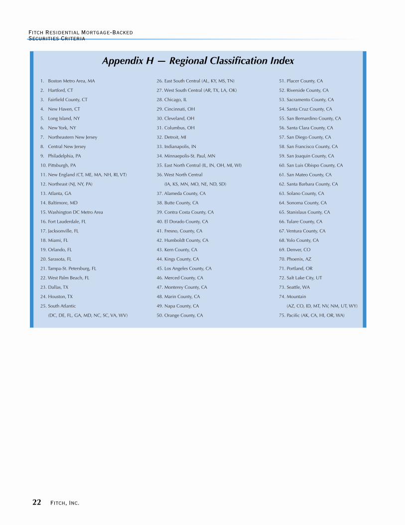
Appendix H — Regional Classification Index


22 Fitch, Inc.


Fitch, Inc. 23

Copyright © 1998 by Fitch IBCA, Inc., One State Street Plaza, NY, NY 10004 Telephone: New York, 1-800-753-4824, (212) 908-0500, Fax (212) 480-4435; Chicago, IL, 1-800-483-4824, (312) 214-3434, Fax (312) 214-3110;London, 011 44 171 638 3800, Fax 011 44 171 374 0103; San Francisco, CA, 1-800-953-4824, (415) 732-5770, Fax (415) 732-5610John Forde, Publisher; Madeline O’Connell, Director, Subscriber Services; Nicholas T. Tresniowski, Senior Managing Editor; Diane Lupi, Managing Editor; JenniferHickey, Andrew Simpson, Igor Zaslavsky, Editors; Martin E. Guzman, Paula M. Sirard, Senior Publishing Specialists; Harvey Aronson, Publishing Specialist; YvonneY. Pak, Robert Rivadeneira, Publishing Assistants. Printed by American Direct Mail Co., Inc. NY, NY 10014. Reproduction in whole or in part prohibited exceptby permission.Fitch IBCA ratings are based on information obtained from issuers, other obligors, underwriters, their experts, and other sources Fitch IBCA believes to be reliable.Fitch IBCA does not audit or verify the truth or accuracy of such information. Ratings may be changed, suspended, or withdrawn as a result of changes in, or theunavailability of, information or for other reasons. Ratings are not a recommendation to buy, sell, or hold any security. Ratings do not comment on the adequacyof market price, the suitability of any security for a particular investor, or the tax-exempt nature or taxability of payments made in respect to any security. FitchIBCA receives fees from issuers, insurers, guarantors, other obligors, and underwriters for rating securities. Such fees generally vary from $1,000 to $750,000 perissue. In certain cases, Fitch IBCA will rate all or a number of issues issued by a particular issuer, or insured or guaranteed by a particular insurer or guarantor,for a single annual fee. Such fees are expected to vary from $10,000 to $1,500,000. The assignment, publication, or dissemination of a rating by Fitch IBCA shallnot constitute a consent by Fitch IBCA to use its name as an expert in connection with any registration statement filed under the federal securities laws. Due tothe relative efficiency of electronic publishing and distribution, Fitch IBCA Research may be available to electronic subscribers up to three days earlier than printsubscribers.


24 Fitch, Inc.

fitch residential mortgage-backed securities criteria

Documents