fitting and evaluating logistic regression models - sas · fitting and evaluating logistic...

#AnalyticsXC o p y r ig ht © 201 6, SAS In st i tute In c. A l l r ig hts r ese rve d.

Fitting and Evaluating Logistic Regression Models

Bruce LundConsultantMagnify Analytic Solutions, a Division of Marketing Associates

#analyticsx

C o p y r ig ht © 201 6, SAS In st i tute In c. A l l r ig hts r ese rve d.

1

Talk focuses on using logistic model for prediction (not explanation) … Topics apply to CRM and Credit Models … but also to other Models.

List of Topics:Binning of discrete predictor variables before modelingTransforming continuous predictor variables before modelingFitting multiple candidate models and ranking by SBC

Correcting SBC for d.f. when using weight-of-evidence

Evaluating and comparing models on validation sample Measures of fit and predictive accuracy

Audience: Current users of logistic regression who are getting started or adding skills.


#analyticsx


2

Assume enough data to have training, validation, and test data sets. (Test data for last step to measure final model performance.)

Omitted Topics:

Stratified Sampling to Reduce the Number of Non-Events

Multicollinearity

Testing of coefficients, discussion of odds-ratios, and, generally, anything that is explanatory

Goodness-of-fit statistics

And more topics …


#analyticsx


3

Terminology … NOD and Continuous Predictors

A Nominal Predictor has values that are not orderede.g. Occupation, University attended … Is U. of Michigan > MSU ?

An Ordinal Predictor has ordered values without an interval scale

e.g. Satisfaction measured as “good”, “fair” “poor”

A Discrete Predictor has numeric values but only a “few” distinct values.e.g. Count of children in household

LEVELS refers to distinct values.

NOD’s appear as CLASS in PROC LOGISTIC; CLASS C; MODEL Y = C <X’s>

A Continuous Predictor is numeric with “lots” of levels … dollars, distance

#analyticsx


4

X Y = 0 Y = 1Col %Y = 0

Col %Y = 1

WOE= Log(%Y=1/%Y=0)

X=X1 2 3 0.400 0.429 0.0690X=X2 1 3 0.200 0.429 0.7621X=X3 2 1 0.400 0.143 -1.0296SUM 5 7 1.000 1.000

X: Predictor Y: Target (response)

Weight of Evidence Coding of X (a NOD)

No “zero cells”

If X = X3 then X_woe = -1.0296

#analyticsx


5

-1.5-1

-0.50

0.51

X=X1 X=X2 X=X3

WO

E

X vs. WOE

Goods are weak

at X3Goods and BadsY = 1 is a “good”, Gi = # goods at Xi, G = total # of goodsY = 0 is a “bad”, Bi = # bads at Xi, B = total # of bads

• Gi / Bi gives that “odds” at Xi

• Log (Gi / Bi) is the “log-odds”

• WOE(Xi) = Log(Gi / Bi) - Log (G / B)

• If WOE(Xi) < 0, then Goods are weak at Xi … relative to Population

WOE – a good way to study X vs. Y

Quadratic relationshipBetween X and WOE ?

#analyticsx


6

PROC LOGISTIC with X_woe (… X a NOD predictor)

DATA WORK;

INPUT Y X$ X_woe F;

DATALINES;

0 X1 0.0690 2

1 X1 0.0690 3

0 X2 0.7621 1

1 X2 0.7621 3

0 X3 -1.0296 2

1 X3 -1.0296 1

;

PROC LOGISTIC DATA = work DESC;MODEL Y = X_woe; FREQ F;

Max Likelihood Estimates

Parameter Estimate

Intercept 0.3365

X_woe 1.0000

Model Fit

Statistics

-2 Log L 15.048

c 0.671

α=log(G/B) and β=1

G = count of Y=1 B = count of Y=0G = 7, B = 5 and log(7/5) = 0.3365

True for MODEL Y = X_woe

#analyticsx


7

PROC LOGISTIC DATA = work DESC;CLASS X (PARAM = REF REF = "X3");MODEL Y = X; FREQ F;

PROC LOGISTIC with CLASS X (… X a NOD predictor)

Maximum Likelihood

EstimatesParameter DF Estimate

Intercept 1 -0.6931

X X1 1 1.0986

X X2 1 1.7918

DATA WORK;

INPUT Y X$ F;

DATALINES;

0 X1 2

1 X1 3

0 X2 1

1 X2 3

0 X3 2

1 X3 1

;

Model Fit

Statistics

-2 Log L 15.048

c 0.671

/*PARAM=REF REF=“X3” tells us how to score an observation when X = “X3”*/

Same fit as Model with woe X

#analyticsx


8

Class (Dummy) compared to Woe coding(A) PROC LOGISTIC; CLASS C1 C2; MODEL Y = C1 C2 <other X’s>;

(B) PROC LOGISTIC; MODEL Y = C1_woe C2_woe <other X’s>;

• Log-likelihood (A) ≥ Log-likelihood (B) … better fit for (A)

Greater LL is due to dummy coefficients “reacting” to other predictors

Single coefficient of a WOE predictor can only rescale the WOE values

• But probabilities from (A) and (B) are usually very similar … especially if multicollinearity is controlled (… in this case LL(A) ~ LL(B))

Choice of (A) or (B) not decisive … good model fit with dummies or WOE.

WOE is popular in credit modeling where it leads to scorecards. It is fully integrated in the Credit Scoring application in SAS® Enterprise Miner.

#analyticsx


9

Binning (collapsing) of a NOD predictorRegardless of (A) or (B) … NOD predictor X should be binned before modeling.

e.g. If 4 levels {R}, {S}, {T}, {U} then bin (collapse) R and T to form {R,T}, {S}, {U}

X with many levels is not parsimonious (over-fitting) … reduce by binning.

• For ordered X:

Binning may reveal useful non-monotonic pattern of X vs. Woe

Business may require X vs. Woe to be monotonic. Binning is used.

Binning X reduces predictive power (=Information Value) of X v. target Y

Good news: there (usually) is a Win-Win:

Predictive power usually decreases very little during early stages of binning if binning is done “optimally” … But how is this done?

#analyticsx


10

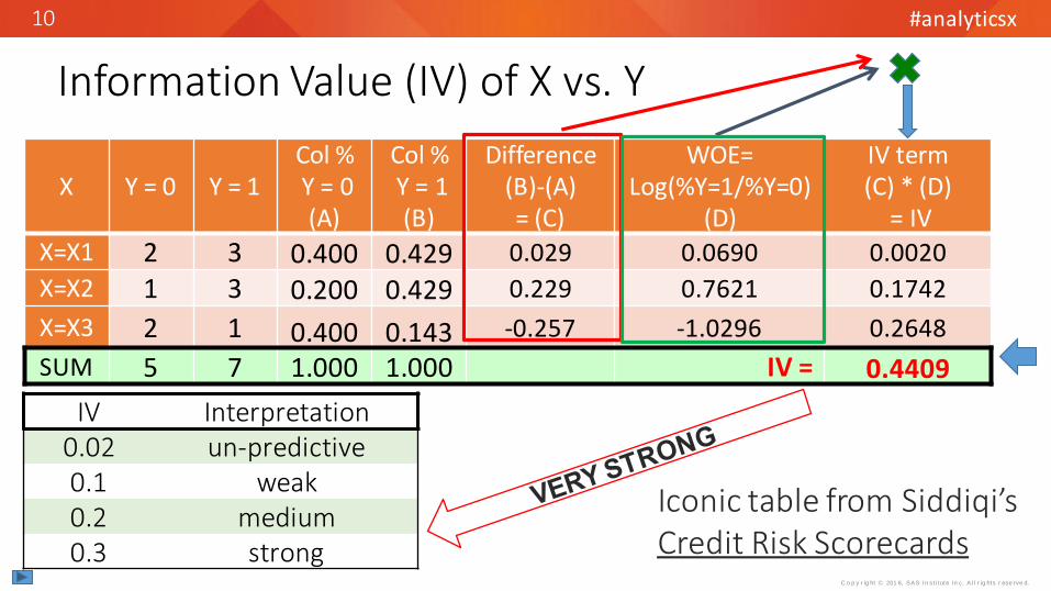
X Y = 0 Y = 1Col %Y = 0(A)

Col %Y = 1(B)

Difference(B)-(A)= (C)

WOE= Log(%Y=1/%Y=0)

(D)

IV term(C) * (D)

= IV

X=X1 2 3 0.400 0.429 0.029 0.0690 0.0020

X=X2 1 3 0.200 0.429 0.229 0.7621 0.1742

X=X3 2 1 0.400 0.143 -0.257 -1.0296 0.2648

SUM 5 7 1.000 1.000 IV = 0.4409

Information Value (IV) of X vs. Y

IV Interpretation0.02 un-predictive0.1 weak0.2 medium0.3 strong

Iconic table from Siddiqi’s Credit Risk Scorecards

#analyticsx


11

Approaches for Binning a NOD X vs. binary Y

Two Approaches:

1. Find two bins to collapse that give maximum IV after collapsing versus all other choices … top down.

2. Decision tree. Find a bin (= branch) to split so that this split maximizes IV versus all other choices … bottom up.

Instead of IV for (1) and (2):

• Entropy (= - log likelihood / n) … this is entropy base “e”

‒ Log Likelihood is from PROC LOGISTIC; CLASS X; MODEL Y = X

• Chi-Sq “p” for measuring independence of X and Y

#analyticsx


12

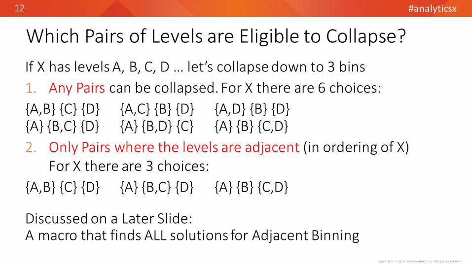
Which Pairs of Levels are Eligible to Collapse?

If X has levels A, B, C, D … let’s collapse down to 3 bins

1. Any Pairs can be collapsed. For X there are 6 choices:

{A,B} {C} {D} {A,C} {B} {D} {A,D} {B} {D}{A} {B,C} {D} {A} {B,D} {C} {A} {B} {C,D}

2. Only Pairs where the levels are adjacent (in ordering of X)For X there are 3 choices:

{A,B} {C} {D} {A} {B,C} {D} {A} {B} {C,D}

Discussed on a Later Slide:A macro that finds ALL solutions for Adjacent Binning

#analyticsx


13

Comments

Splitting with Entropy can give different binning than does Collapsing with Entropy. Here is an example with Adjacent Binning.

A B C D

A_B

A BA_B C_D

A B C D

C_DA_B

A_B_C_D

A_B_C_D

C_D

C D

Collapsing Splitting

#analyticsx


14

Comments

• Collapsing by IV (or LL): Optimal collapse at “k” can lead to sub-optimal status at “k-1”. Here is an example with Adjacent Binning.

A B C D

A_B C D

A_B C_D

IV = .8

IV = .7

IV = .4

A B C D

C_DA B

B_C_D

IV = .8

IV = .6

IV = .5A

4

3

2

Max IV at k=3 but Sub-optimal at k=2 Sub-optimal at k=3, Optimal at k=2

#analyticsx


15

Macro %NOD_BIN

k IV Model cEntropy= -LL/n

L1 L2 L3 L4

4 0.623 0.70 0.614 A B C D3 0.618 0.69 0.615 A+B C D2 0.586 0.68 0.617 A+B C+D

(1) Specify: › All pairs can be collapsed… OR› Only adjacent levels (in ordering of X)(2) Find a pair to collapse to Maximize IV (or LL) at each step

(4) Guidelines for “stopping”:• Big decrease in IV or IV is too small• Quasi statistical tests (not discussed)• Subjective feel

(3) Collapses “small” bins first: • If bin < 5%, find best IV solution to

collapse this bin with another bin• Continue until no more bins < 5%.

Y

X 0 1

A 8 6

B 8 5

C 2 5

D 2 9

Provides WOE Statements: for k = 3

if X in ( "A","B" ) then X_woe = -0.59784 ;

if X in ( "C" ) then X_woe = 0.69315 ;

if X in ( "D" ) then X_woe = 1.28093 ;

#analyticsx


16

Binning Ordered X (with L levels) versus binary YOften a monotonic (vs. WOE) solution is desired or required. See graphLook at k Bins (L ≥ k ≥ 2). The following can happen:

Best IV solution may not be monotonic May be no monotonic solutions May be multiple monotonic solutions

A Challenge: Find best IV (or LL) solution which is monotonic … and do this for each # of bins from L to 2

-3.0-2.0-1.00.01.02.0

1 2 3 4 5 6

WO

E

X

Monotonic decreasing WOE

Here is a monotonic solution for 6 bins but it may not have highest IV among 6 bin solutions.

#analyticsx


17

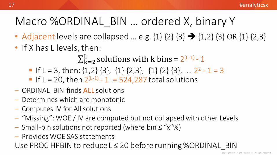
Macro %ORDINAL_BIN … ordered X, binary Y• Adjacent levels are collapsed … e.g. {1} {2} {3} {1,2} {3} OR {1} {2,3}

• If X has L levels, then: k=2

L solutions with k bins = 2(L-1) - 1

If L = 3, then: {1,2} {3}, {1} {2,3}, {1} {2} {3}, … 22 - 1 = 3 If L = 20, then 2(L-1) - 1 = 524,287 total solutions

‒ ORDINAL_BIN finds ALL solutions‒ Determines which are monotonic‒ Computes IV for All solutions ‒ “Missing”: WOE / IV are computed but not collapsed with other Levels ‒ Small-bin solutions not reported (where bin ≤ “x”%)‒ Provides WOE SAS statementsUse PROC HPBIN to reduce L ≤ 20 before running %ORDINAL_BIN

#analyticsx


18

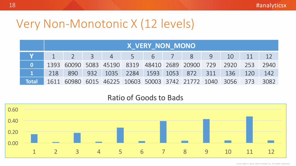
Very Non-Monotonic X (12 levels)

X_VERY_NON_MONO

Y 1 2 3 4 5 6 7 8 9 10 11 12

0 1393 60090 5083 45190 8319 48410 2689 20900 729 2920 253 29401 218 890 932 1035 2284 1593 1053 872 311 136 120 142

Total 1611 60980 6015 46225 10603 50003 3742 21772 1040 3056 373 3082

0.00

0.20

0.40

0.60

1 2 3 4 5 6 7 8 9 10 11 12

Ratio of Goods to Bads

#analyticsx


19

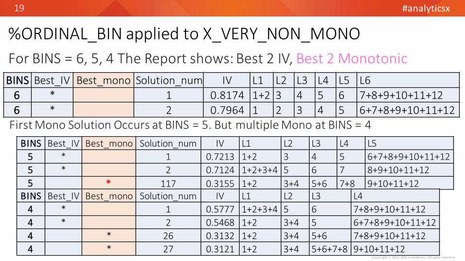
%ORDINAL_BIN applied to X_VERY_NON_MONO

BINS Best_IV Best_mono Solution_num IV L1 L2 L3 L4 L5 L6

6 * 1 0.8174 1+2 3 4 5 6 7+8+9+10+11+12

6 * 2 0.7964 1 2 3 4 5 6+7+8+9+10+11+12

BINS Best_IV Best_mono Solution_num IV L1 L2 L3 L4 L5

5 * 1 0.7213 1+2 3 4 5 6+7+8+9+10+11+12

5 * 2 0.7124 1+2+3+4 5 6 7 8+9+10+11+12

5 * 117 0.3155 1+2 3+4 5+6 7+8 9+10+11+12BINS Best_IV Best_mono Solution_num IV L1 L2 L3 L4

4 * 1 0.5777 1+2+3+4 5 6 7+8+9+10+11+12

4 * 2 0.5468 1+2 3+4 5 6+7+8+9+10+11+12

4 * 26 0.3132 1+2 3+4 5+6 7+8+9+10+11+12

4 * 27 0.3121 1+2 3+4 5+6+7+8 9+10+11+12

First Mono Solution Occurs at BINS = 5. But multiple Mono at BINS = 4

For BINS = 6, 5, 4 The Report shows: Best 2 IV, Best 2 Monotonic

#analyticsx


20

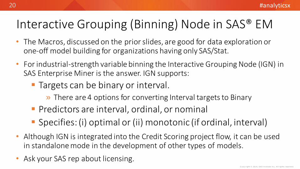
Interactive Grouping (Binning) Node in SAS® EM• The Macros, discussed on the prior slides, are good for data exploration or

one-off model building for organizations having only SAS/Stat.

• For industrial-strength variable binning the Interactive Grouping Node (IGN) in SAS Enterprise Miner is the answer. IGN supports:

Targets can be binary or interval.» There are 4 options for converting Interval targets to Binary

Predictors are interval, ordinal, or nominal

Specifies: (i) optimal or (ii) monotonic (if ordinal, interval)

• Although IGN is integrated into the Credit Scoring project flow, it can be used in standalone mode in the development of other types of models.

• Ask your SAS rep about licensing.

#analyticsx


21

Screening NOD Predictors

Before Binning: NOD predictors are screened to remove weak predictors.

• SAS EM IGN screens by IV

• Here are references for SAS macros that do NOD predictor screening

Lin (2015). Entropy-based Measures of Weight of Evidence and Information Value for Variable Reduction and Segmentation for Continuous Dependent Variables, SGF 2015, 3242-2015

Lund (2015). Fitting and Evaluating Logistic Regression Models, MWSUG 2015, AA03-2015

#analyticsx


22

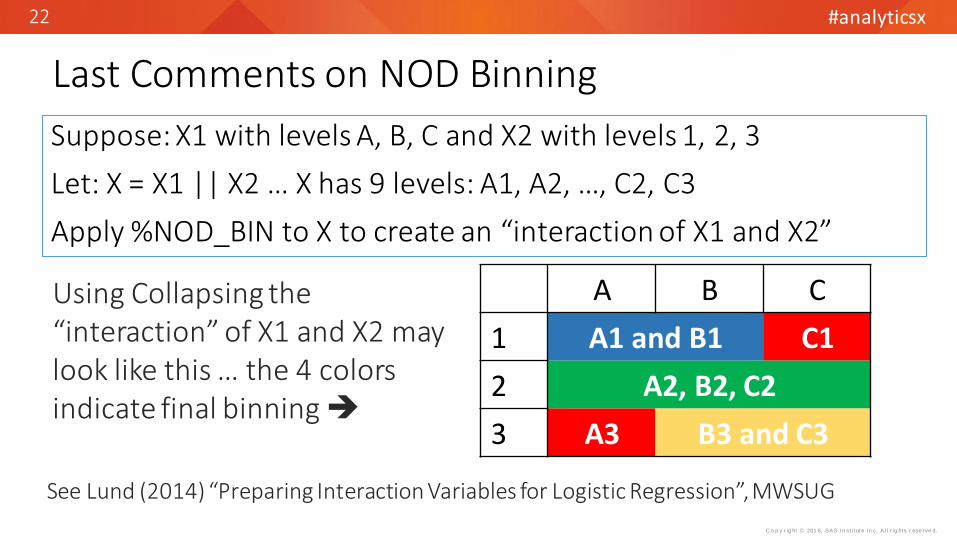
Last Comments on NOD Binning

Suppose: X1 with levels A, B, C and X2 with levels 1, 2, 3

Let: X = X1 || X2 … X has 9 levels: A1, A2, …, C2, C3

Apply %NOD_BIN to X to create an “interaction of X1 and X2”

A B C

1 A1 and B1 C1

2 A2, B2, C2

3 A3 B3 and C3

Using Collapsing the “interaction” of X1 and X2 may look like this … the 4 colors indicate final binning

See Lund (2014) “Preparing Interaction Variables for Logistic Regression”, MWSUG

#analyticsx


23

Should Continuous Predictors be Binned?Usually, effective … but some reasons for NOT binning are: Small sample size A trend but with high variability …

binning may hide the trend False discontinuity of predictor to log-

odds (*) Adds many d.f. to modelSum-up: (i) Overfitting, (ii) Interpretability

Instead: Function Selection Procedure

0.0

0.2

0.4

0.6

0.8

1.0

1.2

1 2 3 4 5 6 7 8 9 10 11 12

Log-odds(Y)

X X_cut3

120 140 160

(*) X =blood pressure vs. Y =heart disease. Cut at X=140 creates “jump” in effect on Y.

#analyticsx


24

Function Selection Procedure (FSP)

FSP is applied to a continuous predictor for logistic regression to select a final transform or to eliminate the predictor from further consideration.

• Multivariate Model-building (2008) by Royston & Sauerbrei (R-S). Also Applied Logistic Regression 3rd by Hosmer, Lemeshow, Sturdivant

• FSP was developed in the middle 1990’s. Bio-medical app’s.

• There are no (few?) papers that discuss FSP for model building for direct marketing or credit scoring.

A summary of FSP is given in the Appendix

• Includes discussion of SAS macros to run FSP

#analyticsx


25

Finding Candidate Models for Logistic Regression

• If K Predictors, there are 2K – 1 possible models.

K = 10 possible models = 1,023

• GOAL: Find a subset “M” of the 2K – 1 which are “good”

• Good will be defined by the Schwarz Bayes Criterion (SBC) … a “penalized measure of fit”

SBC = - 2 * LL + log(n)* K

where LL is log likelihood of model, K is d.f. (= parameters in model including intercept) and n is sample size.

#analyticsx


26

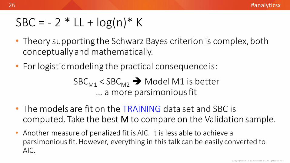
SBC = - 2 * LL + log(n)* K

• Theory supporting the Schwarz Bayes criterion is complex, both conceptually and mathematically.

• For logistic modeling the practical consequence is:

SBCM1 < SBCM2Model M1 is better … a more parsimonious fit

• The models are fit on the TRAINING data set and SBC is computed. Take the best M to compare on the Validation sample.

• Another measure of penalized fit is AIC. It is less able to achieve a parsimonious fit. However, everything in this talk can be easily converted to AIC.

#analyticsx


27

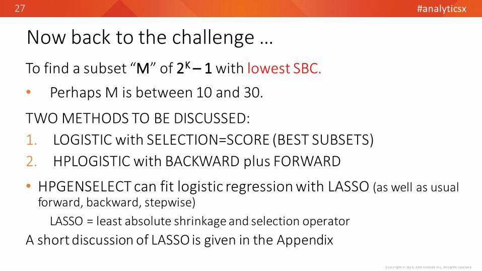
Now back to the challenge …

To find a subset “M” of 2K – 1 with lowest SBC.

• Perhaps M is between 10 and 30.

TWO METHODS TO BE DISCUSSED:

1. LOGISTIC with SELECTION=SCORE (BEST SUBSETS)

2. HPLOGISTIC with BACKWARD plus FORWARD

• HPGENSELECT can fit logistic regression with LASSO (as well as usual forward, backward, stepwise)

LASSO = least absolute shrinkage and selection operator

A short discussion of LASSO is given in the Appendix

#analyticsx


28

PROC LOGISTIC, Score Chi-Square, Selection=Score

Testing Global Null Hypothesis: BETA=0

Test Chi-Square DFPr >

ChiSqLikelihood Ratio 48.9721 2 <.0001

Score 48.6156 2 <.0001Wald 45.9677 2 <.0001

Score chi-sq. is obtained without solving for maximum log likelihood (LL) … this is a short-cut exploited by SELECTION=SCORE.

Next slide …

Score Chi-Sq ~ Likelihood Ratio

#analyticsx


29

PROC LOGISTIC and SELECTION=SCORE (All Subsets)

How do we specify SELECTION=SCORE?

PROC LOGISTIC; MODEL Y=<X’s> / SELECTION=SCORE START=s1 STOP=s2 BEST=b;

START=s1, STOP=s2, BEST=b determine the Models produced

» Each k (predictors) in [s1, s2], find “b” models with greatest Score chi-sq. • For each model we get only:

» Score chi-square and Variables in Model (but no coefficients or LL)

If 4 predictors, X1 – X4 and START=1, STOP=4, and BEST=3, then 10 models are selected:

1 Variable Models: {X1}, {X2}, {X3}, {X4}, take 3 with highest score chi-sq.2 Variable Models: {X1 X2}, {X1 X3}, {X1 X4}, {X2 X3}, {X2 X4}, {X3 X4}, take 3 with highest score chi-sq.3 Variable models: {X1 X2 X3}, {X1 X2 X4}, {X1 X3 X4}, {X2 X3 X4}, take 3 with highest score chi-sq.4 Variable model: {X1 X2 X3 X4}, take the 1 model

#analyticsx


30

PROC LOGISTIC and SELECTION=SCORE (All Subsets)

• But without LL, there is no SBCfor ranking Models.

• A substitute for SBC is “ScoreP”, a penalized Score Chi-Sq

ScoreP = -Score Chi-Sq + log(n) * K … where K = d.f.

• If all 2K – 1 models are ranked by ScoreP and SBC, then:

• No guarantee that rankings are same• But will be very similar.

• For preliminary screening, ScoreP is OK

• See Appendix for connection between ScoreP and SBC

#analyticsx


31

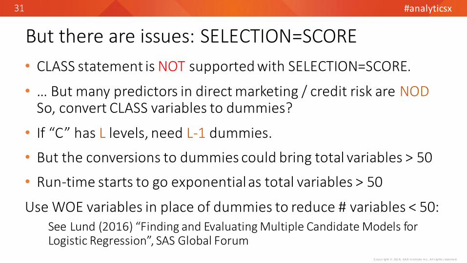
But there are issues: SELECTION=SCORE

• CLASS statement is NOT supported with SELECTION=SCORE.

• … But many predictors in direct marketing / credit risk are NODSo, convert CLASS variables to dummies?

• If “C” has L levels, need L-1 dummies.

• But the conversions to dummies could bring total variables > 50

• Run-time starts to go exponential as total variables > 50

Use WOE variables in place of dummies to reduce # variables < 50:See Lund (2016) “Finding and Evaluating Multiple Candidate Models for Logistic Regression”, SAS Global Forum

#analyticsx


32

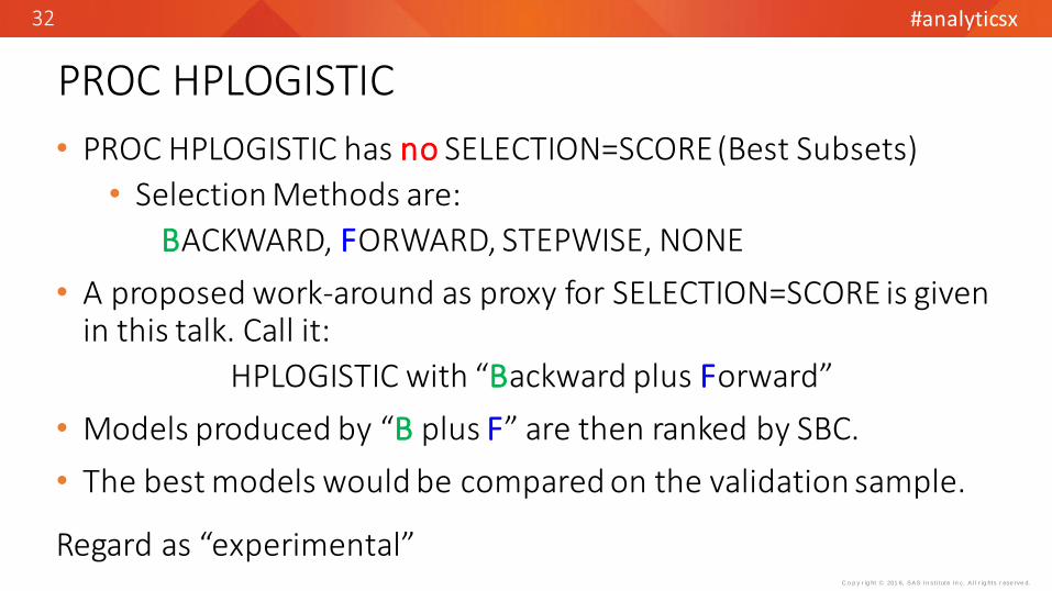
PROC HPLOGISTIC

• PROC HPLOGISTIC has no SELECTION=SCORE (Best Subsets)

• Selection Methods are:

BACKWARD, FORWARD, STEPWISE, NONE

• A proposed work-around as proxy for SELECTION=SCORE is given in this talk. Call it:

HPLOGISTIC with “Backward plus Forward”

• Models produced by “B plus F” are then ranked by SBC.

• The best models would be compared on the validation sample.

Regard as “experimental”

#analyticsx


33

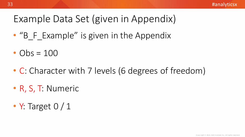
Example Data Set (given in Appendix)

• “B_F_Example” is given in the Appendix

• Obs = 100

• C: Character with 7 levels (6 degrees of freedom)

• R, S, T: Numeric

• Y: Target 0 / 1

#analyticsx


34

HPLOGISTIC with B plus F

ods output SelectionDetails = seldtl_b; ods output CandidateDetails = candtl_b;

PROC HPLOGISTIC DATA= B_F_Example; CLASS C;

MODEL Y (descending) = C R S T;

SELECTION METHOD=BACKWARD

(SELECT = SBC CHOOSE = SBC STOP = NONE) DETAILS=ALL;

DATA canseldtl_b; MERGE seldtl_b candtl_b; BY step;

PROC PRINT DATA= canseldtl_b;

Variables Removed by BackwardOther Candidates for Removal

SELECT=SBC: Finds the X which gives the smallest SBC if X is removed.

#analyticsx


35

Models from Backward

StepNumberIn Model Removed Candidates SBC after removal

1 4 C C 122.821 4 C R 141.301 4 C S 141.451 4 C T 141.602 3 T T 124.502 3 T S 125.202 3 T R 127.483 2 S S 124.833 2 S R 128.164 1 R R 127.74

#analyticsx


36

Models from Backward vs. All Models

Step 0 full Step 1 Step 2 Step 3 Step 4

C R S T R S T S T T null

C S T R S R

C R T R T S

C R S C R C

C S

C T

1 4 3 2 =10

Var. removal in order: C, R, S, T

• Top row are MODELs after Removal

• Blue on white are other “candidates”

• Black on pink are other models

Backward: 1+ (K + … + 2) = (K+1)*K/2 ALL = 2K – 1

#analyticsx


37

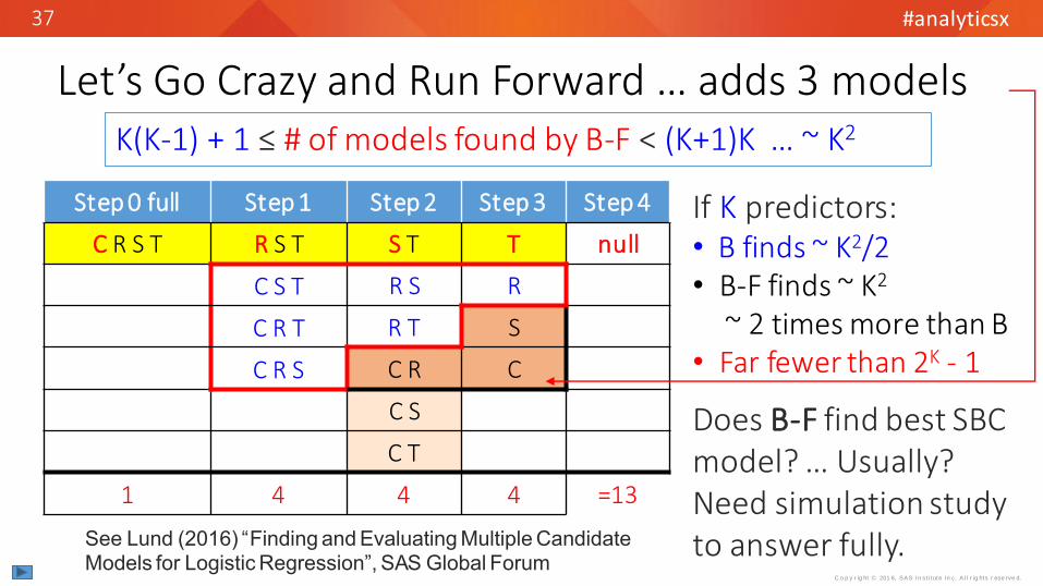
Let’s Go Crazy and Run Forward … adds 3 models

Step 0 full Step 1 Step 2 Step 3 Step 4

C R S T R S T S T T null

C S T R S R

C R T R T S

C R S C R C

C S

C T

1 4 4 4 =13

If K predictors: • B finds ~ K2/2 • B-F finds ~ K2

~ 2 times more than B• Far fewer than 2K - 1

Does B-F find best SBC model? … Usually? Need simulation study to answer fully.

K(K-1) + 1 ≤ # of models found by B-F < (K+1)K … ~ K2

See Lund (2016) “Finding and Evaluating Multiple Candidate Models for Logistic Regression”, SAS Global Forum

#analyticsx


38

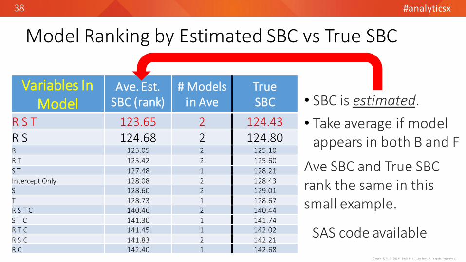
Model Ranking by Estimated SBC vs True SBC

Variables In Model

Ave. Est. SBC (rank)

# Modelsin Ave

TrueSBC

R S T 123.65 2 124.43R S 124.68 2 124.80R 125.05 2 125.10

R T 125.42 2 125.60

S T 127.48 1 128.21

Intercept Only 128.08 2 128.43

S 128.60 2 129.01

T 128.73 1 128.67

R S T C 140.46 2 140.44

S T C 141.30 1 141.74

R T C 141.45 1 142.02

R S C 141.83 2 142.21

R C 142.40 1 142.68

• SBC is estimated.

• Take average if model appears in both B and F

Ave SBC and True SBC rank the same in this small example.

SAS code available

#analyticsx


39

Instead of Class C, the predictor C_woe might be used. This raises an issue when using SBC for ranking models.

C_woe appears to have 1 d.f. but pre-coding of C_woe used entireC * Y table … The new SBC is understated.

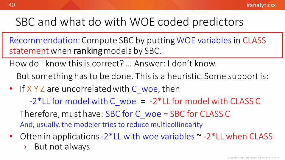
SBC and what do with WOE coded predictors

Variables In Model

Ave. Est. SBC

(rank)

New Ranking (1 d.f.)

Old Ranking

R S T C_WOE 118.426 1 9S T C_WOE 118.676 2 10R S C_WOE 119.408 3 12R T C_WOE 119.443 4 11

What to do ?

#analyticsx


40

Recommendation: Compute SBC by putting WOE variables in CLASSstatement when rankingmodels by SBC.

How do I know this is correct? … Answer: I don’t know.

But something has to be done. This is a heuristic. Some support is:

• If X Y Z are uncorrelated with C_woe, then

-2*LL for model with C_woe = -2*LL for model with CLASS C

Therefore, must have: SBC for C_woe = SBC for CLASS CAnd, usually, the modeler tries to reduce multicollinearity

• Often in applications -2*LL with woe variables ~ -2*LL when CLASS› But not always

SBC and what do with WOE coded predictors

#analyticsx


41

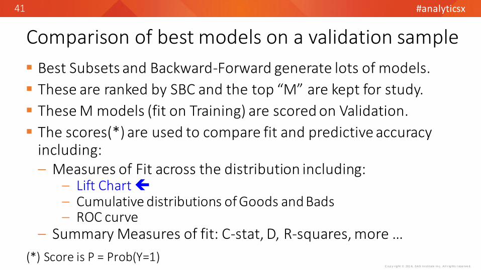
Best Subsets and Backward-Forward generate lots of models.

These are ranked by SBC and the top “M” are kept for study.

These M models (fit on Training) are scored on Validation.

The scores(*) are used to compare fit and predictive accuracy including:‒ Measures of Fit across the distribution including:

‒ Lift Chart ‒ Cumulative distributions of Goods and Bads‒ ROC curve

‒ Summary Measures of fit: C-stat, D, R-squares, more …

Comparison of best models on a validation sample

(*) Score is P = Prob(Y=1)

#analyticsx


42

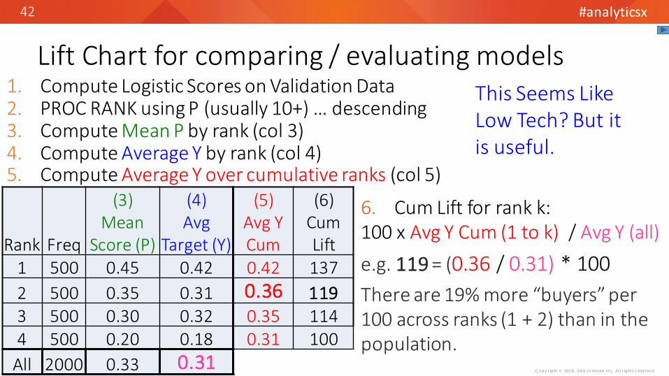
1. Compute Logistic Scores on Validation Data2. PROC RANK using P (usually 10+) … descending3. Compute Mean P by rank (col 3)4. Compute Average Y by rank (col 4)5. Compute Average Y over cumulative ranks (col 5)

Lift Chart for comparing / evaluating models

Rank Freq

(3)Mean

Score (P)

(4)Avg

Target (Y)

(5)Avg YCum

(6)Cum Lift

1 500 0.45 0.42 0.42 137

2 500 0.35 0.31 0.36 1193 500 0.30 0.32 0.35 1144 500 0.20 0.18 0.31 100

All 2000 0.33 0.31

6. Cum Lift for rank k: 100 x Avg Y Cum (1 to k) / Avg Y (all)

e.g. 119 = (0.36 / 0.31) * 100

There are 19% more “buyers” per 100 across ranks (1 + 2) than in the population.

This Seems Like Low Tech? But it is useful.

#analyticsx


43

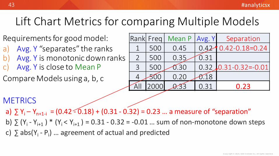
Requirements for good model:a) Avg. Y “separates” the ranksb) Avg. Y is monotonic down ranksc) Avg. Y is close to Mean P

Compare Models using a, b, c

METRICS

Lift Chart Metrics for comparing Multiple Models

Rank Freq Mean P Avg. Y Separation1 500 0.45 0.42 0.42-0.18=0.242 500 0.35 0.313 500 0.30 0.32 0.31-0.32=-0.014 500 0.20 0.18

All 2000 0.33 0.31 0.23

a) ∑ Yi – Yn+1-i = (0.42 - 0.18) + (0.31 - 0.32) = 0.23 … a measure of “separation”

b) ∑ (Yi - Yi+1 ) * (Yi < Yi+1 ) = 0.31 - 0.32 = -0.01 … sum of non-monotone down steps

c) ∑ abs(Yi - Pi) … agreement of actual and predicted

#analyticsx


44

Contact Information

For SAS macros and follow-up questions:

Bruce Lund email addresses:

[email protected] or [email protected]

SAS code discussed:%NOD_BIN%ORDINAL_BINBackward-Forward program%FSP_8LR (Appendix)

mailto:[email protected]

mailto:[email protected]


#analyticsx

#analyticsx


46

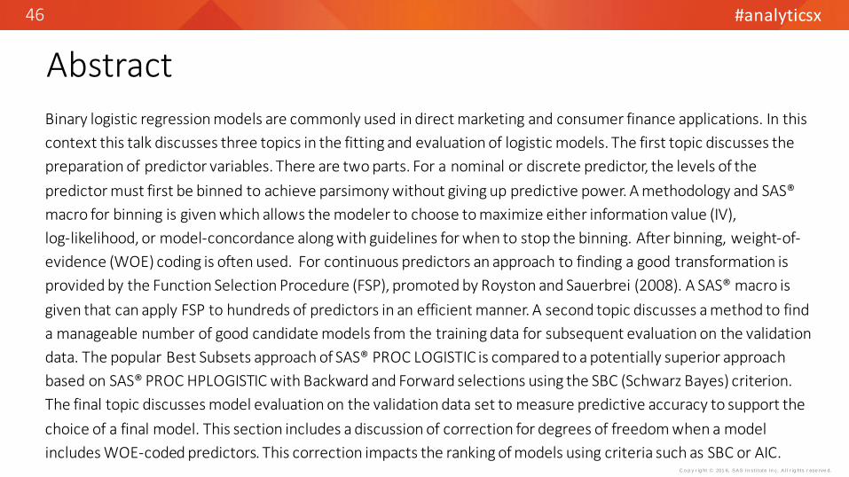
Abstract

Binary logistic regression models are commonly used in direct marketing and consumer finance applications. In this

context this talk discusses three topics in the fitting and evaluation of logistic models. The first topic discusses the

preparation of predictor variables. There are two parts. For a nominal or discrete predictor, the levels of the

predictor must first be binned to achieve parsimony without giving up predictive power. A methodology and SAS®

macro for binning is given which allows the modeler to choose to maximize either information value (IV),

log-likelihood, or model-concordance along with guidelines for when to stop the binning. After binning, weight-of-

evidence (WOE) coding is often used. For continuous predictors an approach to finding a good transformation is

provided by the Function Selection Procedure (FSP), promoted by Royston and Sauerbrei (2008). A SAS® macro is

given that can apply FSP to hundreds of predictors in an efficient manner. A second topic discusses a method to find

a manageable number of good candidate models from the training data for subsequent evaluation on the validation

data. The popular Best Subsets approach of SAS® PROC LOGISTIC is compared to a potentially superior approach

based on SAS® PROC HPLOGISTIC with Backward and Forward selections using the SBC (Schwarz Bayes) criterion.

The final topic discusses model evaluation on the validation data set to measure predictive accuracy to support the

choice of a final model. This section includes a discussion of correction for degrees of freedom when a model

includes WOE-coded predictors. This correction impacts the ranking of models using criteria such as SBC or AIC.

#analyticsx


47

Appendix: B_F_EXAMPLE datasetd at a B_F_Example;

input C$ Y R S T @@;datalines;D 0 11.2 6 0.8 A 1 11.2 6 0.6 D 1 6.7 1 0.6 G 1 9.9 7 0.2 E 0 18.3 6 0.4 A 0 19.7 4 1.0 B 0 8.2 1 0.8 D 0 1.1 3 0.8 B 1 1.4 4 0.0 G 0 16.6 7 1.0 G 0 12.1 3 0.6 A 0 5.0 6 0.8 A 0 7.2 2 0.2 B 0 4.7 3 0.4 A 1 8.2 3 0.0 F 0 15.0 3 0.0 E 1 18.5 6 0.6 C 0 12.0 3 0.8 B 0 16.3 7 0.4 B 1 6.4 4 0.2 A 0 12.4 2 0.4 C 1 18.4 1 0.0 F 0 6.9 4 0.4 F 1 14.8 6 0.6 B 0 11.0 3 0.4 E 0 16.7 1 0.2 F 0 12.0 5 1.0 G 1 15.8 0 0.8 D 1 10.0 4 0.6 G 1 3.8 7 1.0 G 1 9.4 5 0.0 F 0 13.7 7 1.0 F 0 7.8 1 0.8 E 0 9.8 0 0.4 B 1 -0.8 0 0.2 G 1 3.6 7 0.4 G 1 1.3 2 0.6 B 0 11.8 3 0.8 B 0 10.3 2 0.8 A 0 10.2 6 0.6 D 0 8.4 0 0.8 F 0 19.3 3 0.2 A 0 6.3 4 0.2 C 0 3.6 5 0.0 A 0 14.8 4 0.4 B 1 11.4 6 0.2 B 0 2.3 1 0.6 A 0 19.2 7 1.0 G 0 6.2 2 0.8 F 1 8.4 2 0.4 G 1 9.4 2 0.2 G 0 14.0 1 0.6 A 0 18.9 4 0.6 D 1 18.4 6 0.2 B 0 20.6 3 0.6 B 1 5.0 2 0.4 F 0 14.8 1 0.8 B 0 15.3 4 0.6 E 0 16.6 0 0.4 D 0 15.0 2 0.6 C 1 8.4 5 0.0 B 0 14.2 1 0.2 A 0 14.5 5 0.4 E 0 3.6 4 0.4 E 0 13.4 3 0.8 D 0 8.6 2 0.8 B 0 13.7 1 0.4 C 1 9.7 4 0.8 B 0 11.1 2 0.4 C 1 15.6 1 0.6 B 1 -0.8 3 0.4 C 0 11.8 4 0.4 A 0 8.1 4 0.0 D 0 17.5 1 0.0 B 0 18.1 7 0.6 D 0 5.3 1 0.0 B 0 16.0 2 0.0 F 0 20.7 3 0.6 B 1 1.8 6 1.0 F 0 17.6 3 0.6 E 0 12.7 5 0.8 A 0 16.6 3 0.8 C 1 4.3 6 0.4 B 1 7.1 7 0.6 B 0 15.8 2 0.0 D 0 8.4 4 0.6 D 0 5.8 3 0.2 A 0 5.5 0 0.8 D 0 7.9 6 0.4 B 0 5.7 4 1.0 B 1 6.5 4 0.4 C 0 7.1 0 0.8 C 0 19.3 1 1.0 A 0 17.4 7 0.4 B 0 10.4 2 0.4 A 1 16.9 4 0.2 B 0 15.9 3 0.2 C 0 13.7 0 0.8 A 0 6.4 4 0.4 G 1 11.1 4 0.4 ;ru n;

#analyticsx


48

Appendix: HPGENSELECT with LASSO

#analyticsx


49

HPGENSELECT fits Logistic Regression via LASSO

PROC HPGENSELECT Data=B_F_Example;Class C;Model Y (descending) = C R S T / Distribution= Binary; /*<= logistic*/Selection Method=Lasso (Choose=SBC Stop=None) Details=all;

LASSO fits a logistic model with a constraint on ∑ | β | as shown:

F(β) = min{ -LL(β) + λ * ∑ | β | } … (A)

For large λ, F(β) = -LL(β0, 0 … 0) … the model with only the intercept As λ → 0, X’s enter model 1-at-a-time or in small groups to minimize F(β) At λ = 0 the Lasso model is the usual maximum log likelihood solution

• CLASS variables enter “all” or “none” … (A) is modified, see (1/)

(1/) SAS/STAT® 14.1 User’s Guide High-Performance Procedures, p 316, pp 329-331

#analyticsx


50

LASSO and SBC

If there are K predictors, LASSO gives the order of adding these K predictors. This is similar to “forward selection”

But the coefficients and SBC for LASSO models along this forward path are not the same as from the maximum likelihood solutions

Selection Method = LASSO (Choose=SBC) causes the model with lowest SBC to be flagged.

If lowest SBC model appears late along the path, then the LASSO Model and the Max Likelihood (with same predictors) are about the same.

#analyticsx


51

Step Description # Effects Lambda SBC0 Initial Model 1 1 128.421 R entered 2 0.8 131.402 2 0.64 129.74

Omitted 3 - 45 2 0.3277 126.606 S entered 3 0.2621 129.27

Omitted 7 - 1213 3 0.0550 125.0614 3 0.0440 124.97*15 T entered 4 0.0352 129.2316 4 0.0281 128.6717 C entered 5 0.0225 159.26

Omitted 18 - 3940 5 0.0001 145.09

• Best LASSO model {R, S} is shown in STEP 14.

• Best model from B-F was {R, S, T}. Close 2nd best was {R, S}

• {R, S} from LASSO and B-Fhave different coefficients and SBC’s (124.97 v. 124.68)

• Use LASSO for comparison / confirmation of B-F

Results from LASSO

#analyticsx


52

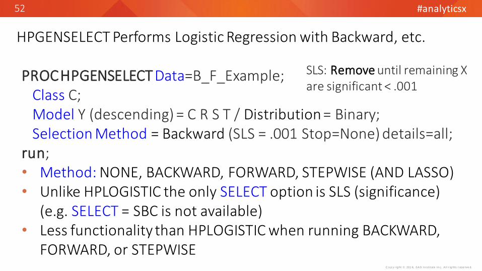
HPGENSELECT Performs Logistic Regression with Backward, etc.

PROCHPGENSELECT Data=B_F_Example;Class C;Model Y (descending) = C R S T / Distribution = Binary;Selection Method = Backward (SLS = .001 Stop=None) details=all;

run;• Method: NONE, BACKWARD, FORWARD, STEPWISE (AND LASSO)• Unlike HPLOGISTIC the only SELECT option is SLS (significance)

(e.g. SELECT = SBC is not available)• Less functionality than HPLOGISTIC when running BACKWARD,

FORWARD, or STEPWISE

SLS: Remove until remaining X are significant < .001

#analyticsx


53

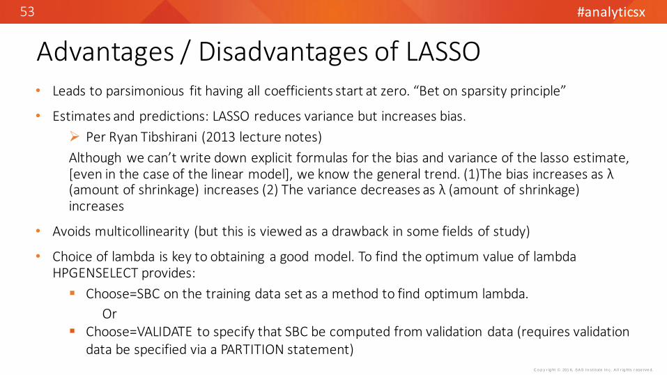
Advantages / Disadvantages of LASSO• Leads to parsimonious fit having all coefficients start at zero. “Bet on sparsity principle”

• Estimates and predictions: LASSO reduces variance but increases bias.

Per Ryan Tibshirani (2013 lecture notes)

Although we can’t write down explicit formulas for the bias and variance of the lasso estimate, [even in the case of the linear model], we know the general trend. (1)The bias increases as λ (amount of shrinkage) increases (2) The variance decreases as λ (amount of shrinkage) increases

• Avoids multicollinearity (but this is viewed as a drawback in some fields of study)

• Choice of lambda is key to obtaining a good model. To find the optimum value of lambda HPGENSELECT provides:

Choose=SBC on the training data set as a method to find optimum lambda.

Or Choose=VALIDATE to specify that SBC be computed from validation data (requires validation

data be specified via a PARTITION statement)

#analyticsx


54

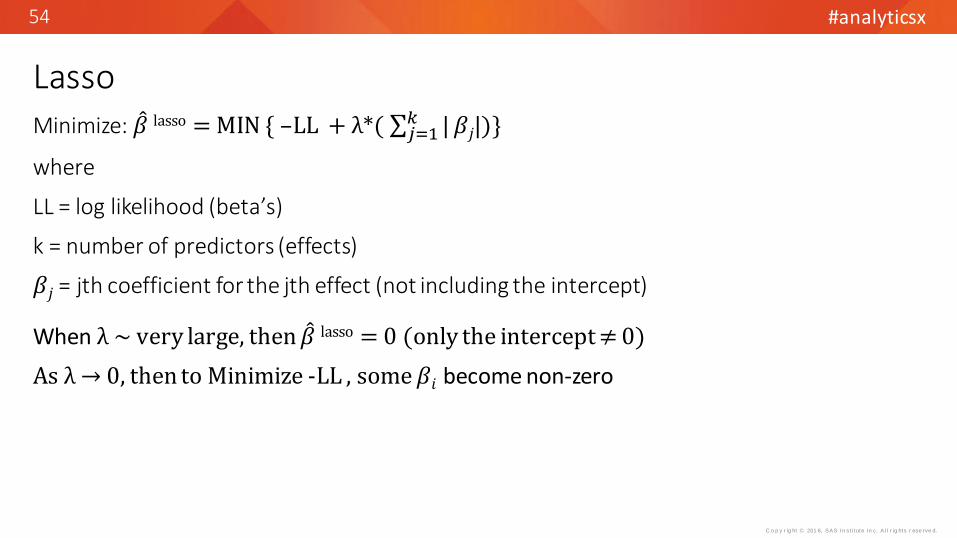
LassoMinimize: 𝛽 lasso = MIN { –LL + λ*( 𝑗=1

𝑘 | 𝛽𝑗|)}

where

LL = log likelihood (beta’s)

k = number of predictors (effects)

𝛽𝑗 = jth coefficient for the jth effect (not including the intercept)

When λ ~ very large, then 𝛽 lasso = 0 (only the intercept ≠ 0)

As λ → 0, then to Minimize -LL , some 𝛽𝑖 become non-zero

#analyticsx


55

Group Lasso

Minimize: 𝛽 lasso = MIN { –LL + λ∗ ( 𝑗=1𝑘 𝐺𝑗

𝑖=1

𝐺𝑗 𝛽𝑖2 )}

where

LL = log likelihood (beta’s)

k = number of predictors (effects)

𝐺𝑗 = number of coefficients in jth effect

𝛽𝑖 = ith coefficient for the jth effect

When λ ~ very large, then 𝛽 lasso = 0 (only the intercept ≠ 0)

As λ → 0, then to Minimize -LL , some 𝛽𝑖 become non-zero

#analyticsx


56

Appendix: FSP

#analyticsx


57

Appendix: FSP

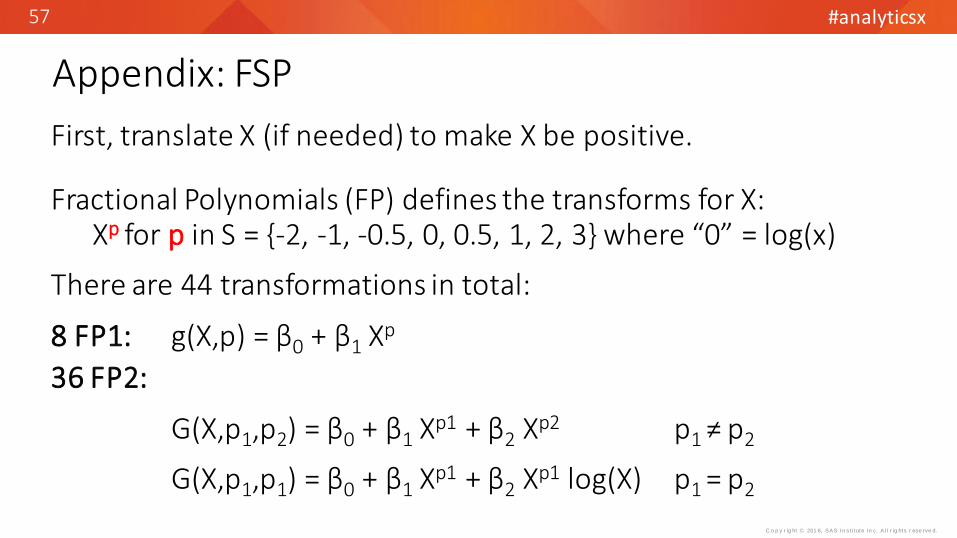
First, translate X (if needed) to make X be positive.

Fractional Polynomials (FP) defines the transforms for X: Xp for p in S = {-2, -1, -0.5, 0, 0.5, 1, 2, 3} where “0” = log(x)

There are 44 transformations in total:

8 FP1: g(X,p) = β0 + β1 Xp

36 FP2:

G(X,p1,p2) = β0 + β1 Xp1 + β2 Xp2 p1 ≠ p2

G(X,p1,p1) = β0 + β1 Xp1 + β2 Xp1 log(X) p1 = p2

#analyticsx


58

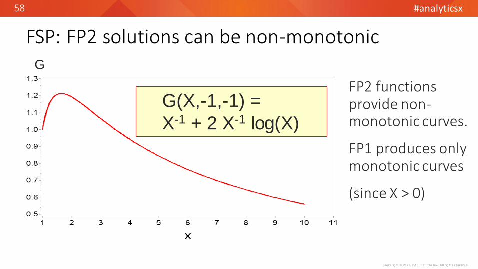
FSP: FP2 solutions can be non-monotonic

G(X,-1,-1) =

X-1 + 2 X-1 log(X)

FP2 functions provide non-monotonic curves.

FP1 produces only monotonic curves

(since X > 0)

G

#analyticsx


59

FSP: Two Main Steps

A SAS macro is provided by R-S via a web-site.

Finds the FP1 and FP2 with best log likelihoods All 44 Logistic Models are run.

Processes only 1 predictor at a time through FSP.

Performs a 3-step test to determine the statistical significance of FP1 and FP2 solutions.

#analyticsx


60

FSP: Significance Test

Test Stat = { - 2Log(L)restricted } - { - 2log(L)full } ~ Chi-Sq.

1. 4 d.f. test at “α” level of best FP2 against null model. If test is not significant, drop X and stop, else continue.

2. 3 d.f. test at “α” of best FP2 against a X (linear). If test is not significant, stop (final model is linear), else continue.

3. 2 d.f. test at “α” of best FP2 vs. best FP1. If test is significant, the final model is the FP2, otherwise it is FP1.

See R-S for discussion of d.f. = 4, 3, 2

#analyticsx


61

Data Set “Example” has 500 observationsdata Example;do i = 1 to 500;

X = ranuni(12341);Y = floor(X + ranuni(12341));output;end;

run;

Distribution of X

Perc

en

t

0.0 0.1 0.2 0.3 0.4 0.5 0.6 0.7 0.8 0.9 1.0

X

0

5

10

15

20

0

5

10

15

20

Y =

1Y

= 0

X

Y=0

Y=1

#analyticsx


62

FSP applied to X (translated: min(X) = 1)

• Based on 3-step test the “solution” is Linear … if using 5%

(FP2 vs. Linear fails at 5% significance … test-stat= 6.105 and α= 10.6%)

• Best FP1 is X-2 and best FP2 is X-2 and X3

Function p1 p2Chi-Sq Test

StatAchieved

αD.F.

Null . . 208.202 0.000% 4Linear . . 6.105 10.658% 3FP1 -2 . 0.644 72.451% 2FP2 -2 3

#analyticsx


63

Linear, FP1, and FP2 Solutions for X

-5

-4

-3

-2

-1

0

1

2

3

1 1.1 1.2 1.3 1.4 1.5 1.6 1.7 1.8 1.9 2

Log-

od

ds(Y

)

X

Log_odds(Y) Linear FP1 FP2

FP1 and FP2 solutions appear to fit Log-Odds(Y) better than does Linear

FP1 = 4.09 - 8.32 X-2

FP2 = 2.97 - 6.95 X-2 + 0.13 X3

Linear = -7.93 + 5.35 X

#analyticsx


64

FSP in SAS

Download FSP SAS macro %MFP8 at:

http://portal.uni-freiburg.de/imbi/mfp

• %MFP8 performs the FSP on a single predictor X

• User must translate X, if needed, so that X > 0.

Better: If min(X) < 1, then make min(X) = 1

• Written in SAS 8. A small fix is needed to run in SAS 9. (*)

• Many useful options. Also performs FSP for OLS and Proportional Hazards Model.

(*) See Lund (2015) “Selection and Transformation of Continuous Predictors for Logistic Regression”, SAS Global Forum

#analyticsx


65

More SAS Macros for FSP

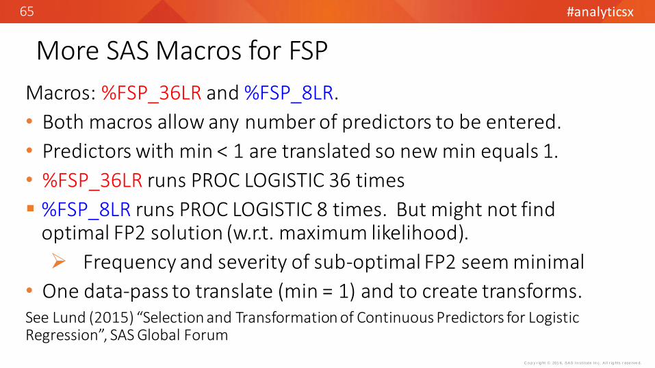
Macros: %FSP_36LR and %FSP_8LR.

• Both macros allow any number of predictors to be entered.

• Predictors with min < 1 are translated so new min equals 1.

• %FSP_36LR runs PROC LOGISTIC 36 times

%FSP_8LR runs PROC LOGISTIC 8 times. But might not find optimal FP2 solution (w.r.t. maximum likelihood).

Frequency and severity of sub-optimal FP2 seem minimal

• One data-pass to translate (min = 1) and to create transforms.See Lund (2015) “Selection and Transformation of Continuous Predictors for Logistic Regression”, SAS Global Forum

#analyticsx


66

Appendix: Other Slides

#analyticsx


67

C-stat measures model accuracy in the following sense:

Given random pair of observations where target=0 and target=1, the c-stat is probability the logistic P is larger when target=1.

An adjustment is made for tied probabilities.

C-statistic from Logistic ModelObs. Y Prob

1 0 0.3

2 0 0.45

3 1 0.4

4 1 0.5

4 “informative pairs”:(1,3), (1,4), (2,3), (2,4)

(1,3) is concordant0.3 < 0.4

(1,4) is concordant(2,3) not(2,4) is concordant

C-stat = 3 / 4

C-stat = (Concordant + .5*Ties)/ Info. Pairs

If a modeler has fit many Models to same or similar Data, then c-stat is useful as a guidepost … “for this type of model I usually get 0.70”

#analyticsx


68

If X has L levels, there are 2(L-1) - 1 adjacent bin solutions

Consider the number of k bin solutions for 2 ≤ k ≤ L. Each of the k bins has a subset of {1, …, L}

Consider the example where L = 5 and k = 3. One solution for k = 3 is {1,2}, {3,4}, {5}.

In general, let C1, C2, C3 refer to the count of levels in each of the 3 bins. Then the number of solutions for k = 3 is the same as the number of positive integer solutions to 5 = C1 + C2 + C3.

And more generally, for X with L levels, the number of k bin solutions is the same as the number of positive integer solutions to

C1 + … + Ck = L … (A)

We first need to solve a related problem. Find the number of nonnegative integer solutions to

C1 + … + Ck = N … (B)

A combinatorial argument is given. List levels 1, 2, …, N in a row and place k-1 vertical bars “|” before, between, or after the levels.

For example, if N = 5, k = 3, then one configuration is 1 | 2 3 4 5 |. This gives a solution to (B) of 1 + 4 + 0 = 5

There are 5+22

= 21 ways to pick 2 positions from 7 to place the “|”. In general, there are 𝑁+𝑘 −1𝑘 −1

solutions

to (B). On the next slide the number of solutions to (A) is found by using the information from (B)

#analyticsx


69

If X has L levels, there are 2(L-1) - 1 adjacent bin solutions … 2

Since N is an arbitrary positive integer, we can define L + k = N (where 1 < k ≤ L) and re-state equation (A) to say:

C1 + … + Ck = L + k … (C)

The number of non-negative solutions to (C) is 𝐿 −1𝑘 −1

Now for the 1-1 correspondence:

Let (x1,…, xk) solve (C). Then (x1 +1, …, xk +1) solves (A).

Conversely, if (y1, …, yk) solves (A), then (y1 -1, …, yk -1) solves (C)

So the number of positive integer solutions to (A) is 𝐿 −1𝑘 −1

where 1 < k ≤ L

Now by the binomial expansion:

1 + 𝑘=2𝐿−1 𝐿 −1

𝑘 −1= 𝑗=1

𝐿−1 𝐿 −1𝑗

= 2(L-1) so that 𝑘=2𝐿−1 𝐿 −1

𝑘 −1= 2(L-1) - 1

#analyticsx


70

D = abs( mean(P_1 | Y=1 ) - mean(P_1 | Y=0 ) ) Tjur (2009) Coefficients of Determination in Logistic Regression …” American StatisticianAllison (2016) “Measures of Fit for Logistic Regression” SGFPROC HPLOGISTIC computes D. See SAS Usage Note 39109

D has these properties:» Easy to compute and to explain» Can compare Model fits for logistic, trees, other methods … not dependent on

how model was fit » 0 ≤ D with “=“ if only if P’s are equal for all obs. (no fit)» D ≤ 1 with “=“ if and only if P = Y for all obs. (perfect fit)

D and R-squares are generally very low for direct marketing models These measures can be useful for model comparison Are there guidelines for what is a “good” D value?

Coefficient of Determination D … a better R-SQ?

#analyticsx


71

Further Comments on Binning

Can %NOD_BIN be re-programmed for complete enumeration (like %ORDINAL_BIN)?

Probably …

• Computationally … If L = 10 there are ~ 100,000 total solutions (Bin = 10, 9, …, 2)

Computationally, a predictor with 10 bins can be processed.

• But SAS coding to generate and evaluate these solutions is the challenge

#analyticsx


72

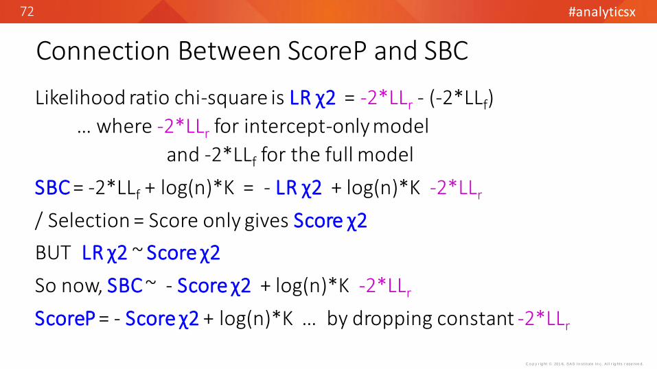
Connection Between ScoreP and SBC

Likelihood ratio chi-square is LR χ2 = -2*LLr - (-2*LLf)

… where -2*LLr for intercept-only model

and -2*LLf for the full model

SBC = -2*LLf + log(n)*K = - LR χ2 + log(n)*K -2*LLr

/ Selection = Score only gives Score χ2

BUT LR χ2 ~ Score χ2

So now, SBC ~ - Score χ2 + log(n)*K -2*LLr

ScoreP = - Score χ2 + log(n)*K … by dropping constant -2*LLr

#analyticsx


73

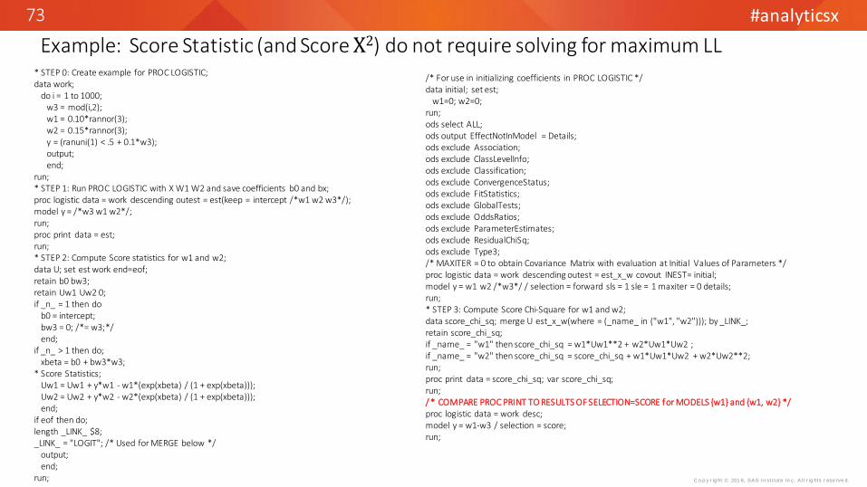
Example: Score Statistic (and Score Χ2) do not require solving for maximum LL* STEP 0: Create example for PROC LOGISTIC;data work;

do i = 1 to 1000;w3 = mod(i,2);w1 = 0.10*rannor(3);w2 = 0.15*rannor(3);y = (ranuni(1) < .5 + 0.1*w3);output;end;

run;* STEP 1: Run PROC LOGISTIC with X W1 W2 and save coefficients b0 and bx;proc logistic data = work descending outest = est(keep = intercept /*w1 w2 w3*/);model y = /*w3 w1 w2*/;run;proc print data = est;run;* STEP 2: Compute Score statistics for w1 and w2;data U; set est work end=eof;retain b0 bw3;retain Uw1 Uw2 0;if _n_ = 1 then do

b0 = intercept;bw3 = 0; /*= w3;*/end;

if _n_ > 1 then do;xbeta = b0 + bw3*w3;

* Score Statistics;Uw1 = Uw1 + y*w1 - w1*(exp(xbeta) / (1 + exp(xbeta))); Uw2 = Uw2 + y*w2 - w2*(exp(xbeta) / (1 + exp(xbeta))); end;

if eof then do;length _LINK_ $8;_LINK_ = "LOGIT"; /* Used for MERGE below */

output;end;

run;

/* For use in initializing coefficients in PROC LOGISTIC */data initial; set est;

w1=0; w2=0;run;ods select ALL;ods output EffectNotInModel = Details;ods exclude Association;ods exclude ClassLevelInfo;ods exclude Classification;ods exclude ConvergenceStatus;ods exclude FitStatistics;ods exclude GlobalTests;ods exclude OddsRatios; ods exclude ParameterEstimates;ods exclude ResidualChiSq; ods exclude Type3;/* MAXITER = 0 to obtain Covariance Matrix with evaluation at Initial Values of Parameters */proc logistic data = work descending outest = est_x_w covout INEST= initial;model y = w1 w2 /*w3*/ / selection = forward sls = 1 sle = 1 maxiter = 0 details;run;* STEP 3: Compute Score Chi-Square for w1 and w2;data score_chi_sq; merge U est_x_w(where = (_name_ in ("w1", "w2"))); by _LINK_;retain score_chi_sq;if _name_ = "w1" then score_chi_sq = w1*Uw1**2 + w2*Uw1*Uw2 ;if _name_ = "w2" then score_chi_sq = score_chi_sq + w1*Uw1*Uw2 + w2*Uw2**2;run;proc print data = score_chi_sq; var score_chi_sq;run;/ * COMPARE PROC PRINT TO RESULTS OF SELECTION=SCORE for MODELS {w1} and {w1, w2} */proc logistic data = work desc;model y = w1-w3 / selection = score;run;

#analyticsx


74

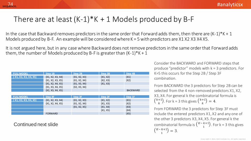
There are at least (K-1)*K + 1 Models produced by B-F

sequence.

In the case that Backward removes predictors in the same order that Forward adds them, then there are (K-1)*K + 1 Models produced by B-F. An example will be considered where K = 5 with predictors are X1 X2 X3 X4 X5.

It is not argued here, but in any case where Backward does not remove predictors in the same order that Forward adds them, the number of Models produced by B-F is greater than (K-1)*K + 1

FULL MODEL Step 1B Step 2B Step 3B Step 4B{ X1, X2, X3, X4, X5} {X1, X2, X3, X4} {X1, X2, X3} {X1, X2} {X1}

{X1, X2, X3, X5} {X1, X2, X4} {X2, X3} {X2}{X1, X2, X4, X5} {X1, X3, X4} {X1, X3}{X1, X3, X4, X5} {X2, X3, X4}{X2, X3, X4, X5} BACKWARD

FULL MODEL Step 4F Step 3F Step 2F Step 1F{ X1, X2, X3, X4, X5} {X1, X2, X3, X4} {X1, X2, X3} {X1, X2} {X1}

{X1, X2, X4, X5} {X1, X2, X4} {X1, X3} {X2}{X1, X2, X5} {X1, X4} {X3}

{X1, X5} {X4}FORWARD {X5}

Consider the BACKWARD and FORWARD steps that produce “predictor” models with k = 3 predictors. For K=5 this occurs for the Step 2B / Step 3F combination.

From BACKWARD the 3 predictors for Step 2B can be selected from the 4 non-removed predictors X1, X2, X3, X4. For general k the combinatorial formula is

𝑘+1𝑘

. For k = 3 this gives 𝑘+1𝑘

= 4.

From FORWARD the 3 predictors for Step 3F must include the entered predictors X1, X2 and any one of the other 3 predictors X3, X4, X5. For general k the

combinatorial formula is 𝐾− 𝑘+11

. For k = 3 this gives 𝐾− 𝑘+1

1= 3.

Continued next slide

#analyticsx


75

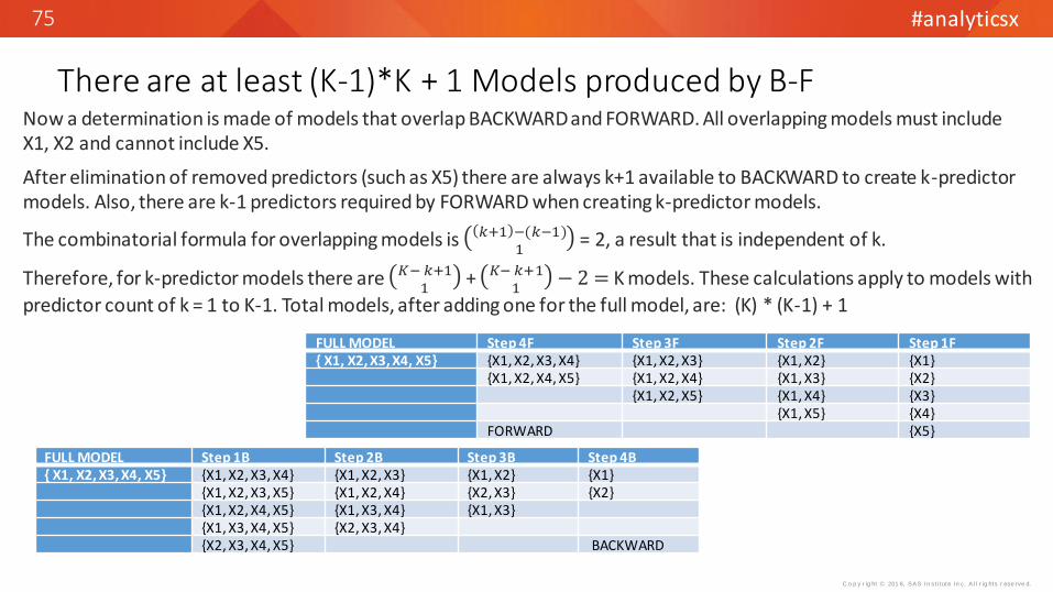
There are at least (K-1)*K + 1 Models produced by B-FNow a determination is made of models that overlap BACKWARD and FORWARD. All overlapping models must include X1, X2 and cannot include X5.

After elimination of removed predictors (such as X5) there are always k+1 available to BACKWARD to create k-predictor models. Also, there are k-1 predictors required by FORWARD when creating k-predictor models.

The combinatorial formula for overlapping models is 𝑘+1 −(𝑘−1)1

= 2, a result that is independent of k.

Therefore, for k-predictor models there are 𝐾− 𝑘+11

+ 𝐾− 𝑘+11

− 2 = K models. These calculations apply to models with

predictor count of k = 1 to K-1. Total models, after adding one for the full model, are: (K) * (K-1) + 1

FULL MODEL Step 1B Step 2B Step 3B Step 4B{ X1, X2, X3, X4, X5} {X1, X2, X3, X4} {X1, X2, X3} {X1, X2} {X1}

{X1, X2, X3, X5} {X1, X2, X4} {X2, X3} {X2}{X1, X2, X4, X5} {X1, X3, X4} {X1, X3}{X1, X3, X4, X5} {X2, X3, X4}{X2, X3, X4, X5} BACKWARD

FULL MODEL Step 4F Step 3F Step 2F Step 1F{ X1, X2, X3, X4, X5} {X1, X2, X3, X4} {X1, X2, X3} {X1, X2} {X1}

{X1, X2, X4, X5} {X1, X2, X4} {X1, X3} {X2}{X1, X2, X5} {X1, X4} {X3}

{X1, X5} {X4}FORWARD {X5}


#AnalyticsX

fitting and evaluating logistic regression models - sas · fitting and evaluating logistic...

Documents