fitting net photosynthetic light-response curves with ... · fitting net photosynthetic...

DOI: 10.1007/s11099-013-0045-y PHOTOSYNTHETICA 51 (3): 445-456, 2013

445

Fitting net photosynthetic light-response curves with Microsoft Excel – a critical look at the models F. de A. LOBO*,+, M.P. de BARROS**, H.J. DALMAGRO**, Â.C. DALMOLIN**, W.E. PEREIRA***, É.C. de SOUZA#, G.L. VOURLITIS##, and C.E. RODRÍGUEZ ORTÍZ### Departamento de Solos e Engenharia Rural, FAMEV/UFMT, 78060-900, Cuiabá-MT, Brasil* Programa de Pós-Graduação em Física Ambiental, IF/UFMT, 78060-900, Cuiabá-MT, Brasil** Departamento de Ciências Fundamentais e Sociais, CCA/UFPB, 58397-000, Areia-PB, Brasil*** Departamento de Estatística, ICET/UFMT, 78060-900, Cuiabá-MT, Brasil# Department of Biological Science, CSUSM, San Marcos-CA, 92096-0001, USA## Departamento de Botânica e Ecologia, IB/UFMT, 78060-900, Cuiabá-MT, Brasil###

Abstract

In this study, we presented the most commonly employed net photosynthetic light-response curves (PN/I curves) fitted by the Solver function of Microsoft Excel. Excel is attractive not only due to its wide availability as a part of the Microsoft Office suite but also due to the increased level of familiarity of undergraduate students with this tool as opposed to other statistical packages. In this study, we explored the use of Excel as a didactic tool which was built upon a previously published paper presenting an Excel Solver tool for calculation of a net photosynthetic/chloroplastic CO2-response curve. Using the Excel spreadsheets accompanying this paper, researchers and students can quickly and easily choose the best fitted PN/I curve, selecting it by the minimal value of the sum of the squares of the errors. We also criticized the misuse of the asymptotic estimate of the maximum gross photosynthetic rate, the light saturation point estimated at a specific percentile of maximum net photosynthetic rate, and the quantum yield at zero photosynthetic photon flux density and we proposed the replacement of these variables by others more directly linked to plant ecophysiology. Additional key words: curve fitting; iteration; nonlinear regression; PN/I curve; Solver function. Introduction

The net photosynthetic light-response curve (PN/I curve) describes the net CO2 assimilation by a plant leaf (PN) as a function of an increase in the photosynthetic photon flux density (I) from the total absence of light to a high

level of light, e.g. 2,000 µmol(photon) m–2 s–1. The curve presents several phases. At the beginning,

from complete darkness to the light compensation point (Icomp), there is a rapid increase in PN with I, due to the

——— Received 17 April 2012, accepted 17 January 2013. +Corresponding author; e-mail: [email protected] Abbreviations: ARE – average relative errors; Cc – chloroplast CO2 concentration; Ci – intercellular CO2 concentration; I – photosynthetic photon flux density; Icomp – light compensation point; Imax – light saturation point beyond which there is no significant change in PN; Isat – light saturation point; Isat(n) – light saturation point at a specific percentile (n) of PNmax; Isat(85) – light saturation point for PN + RD equal to 85% of PNmax; Isat(90) – light saturation point for PN + RD equal to 90% of PNmax; Isat(95) – light saturation point for PN + RD equal to 95% of PNmax; I(50) – light saturation point for PN + RD equal to 50% of PNmax; k – adjusting factor; Pg – gross photosynthetic rate; Pgmax – maximum gross photosynthetic rate; PN – net photosynthetic rate; PN(Imax) – maximum net photosynthetic rate obtained at I = Imax; PNmax – maximum net photosynthetic rate; RD – dark respiration; R2 – coefficient of determination; SAE – sum of the absolute errors; SSE – sum of the squares of the errors; Vmax – enzyme maximum velocity; – adjusting factor; – adjusting factor; – convexity factor; – quantum yield; (I) – quantum yield at a particular value of I; ϕ(Icomp) – quantum yield at I = Icomp; ϕ(Icomp – I200) – quantum yield at the range between Icomp and I = 200 µmol(photon) m–2 s–1; ϕ(I0) – quantum yield at I = 0 µmol(photon) m–2 s–1; ϕ(I0 – Icomp) – quantum yield at the range between I = 0 µmol(photon) m–2 s–1 and

Icomp; max – theoretical maximum quantum yield; χ2 – Chi-square test. Acknowledgments: This study was supported by grants from the Instituto Nacional de Ciência e Tecnologia em Áreas Úmidas (INAU), Programa Institutos Nacionais de Ciência e Tecnologia (CNPq/MCT), and from Fundação de Amparo à Pesquisa do Estado de Mato Grosso (FAPEMAT) and scholarships from Conselho Nacional de Desenvolvimento Cientifico e Tecnológico (CNPq). We would like to thank Dr. Clóvis Nobre de Miranda for allowing us to conduct the research on his farm and for giving us the facilities to work there.

F. de A. LOBO et al.

446

natural decrease in dark respiration (RD), named the Kok effect (Kok 1949). The light compensation point is the value of I at which the CO2 assimilated by photosynthesis is in balance with the CO2 produced by light respiration and photorespiration, resulting in PN equal to zero. Beyond this point, a supposed linear response of PN to I can be seen until I reaches approximately 200 µmol (photon) m–2 s–1. This linear portion is the range that many authors use to calculate the “maximum quantum yield” (ϕ(Icomp – I200)), which is the slope in that range, and beyond this range there is a region of nonlinear die-off before PN reaches a semiplateau, where an increase in I does not provoke a proportional increase in PN (Long and Hällgren 1993). The progressive curvature in the ratio PN/I in this region can be described by a convexity factor () (Ögren 1993). Sometimes, after reaching the maximum value of PN, a subsequent decrease in PN with I, referred to as photoinhibition, can be observed (Ye 2007). Extensive literature is available describing the different phases of the curve and the effects of temperature, CO2 concentration, pH, chemical inhibitors of photosynthesis, and other factors (Long and Hällgren 1993, Govindjee et al. 2005, Zeinalov 2005, Lambers et al. 2008).

Many mathematical models may be used to describe PN/I curves. Various parameters and variables calculated from these models are used to describe the photosynthetic capacity, efficiency, and other aspects. Those variables include Icomp, the asymptotic estimate of the maximum gross photosynthetic rate (Pgmax), the light saturation point for PN + RD equal to 50% of maximum net photosynthetic rate (PNmax) (I(50)), the light saturation point for PN equal to a percentile of the PNmax (Isat(n)), the light saturation point (Isat), the quantum yield at I = 0 µmol(photon) m–2 s–1 (ϕ(I0)), the quantum yield obtained in the range between Io and Icomp (ϕ(I0 – Icomp)), ϕ(Icomp – I200),

obtained at any value of I ((I)), , and RD. Certain models are modifications of the originals, but

sometimes these modifications produce serious problems that are not handled properly or, at best, they produce meaningless information. Kaipiainen (2009) uses a modi-fied Michaelis-Menten model (Eq. 2), assuming that I(50)

is the value of I, when PN is equal to 50% of Pgmax; however, that assumption is only true if the gross photosynthetic rate (Pg, which is equal to PN + RD) is equal to 50% of Pgmax. A nonrectangular hyperbola, in its original form (Eq. 6), was modified by Chen et al. (2008) to give the form of Eq. 7, which produces misleading information about the value of PN in the absence of light (I = 0). In that case, when I = 0, it is expected that PN = –RD, but the modified model produces a value of

Dgmax

N θ2R

PP . The original, exponential model (Eq. 8)

has many different variations. One of these variations can be seen in the papers of Lootens et al. (2004) and Devacht

et al. (2009), shown in Eq. 10, where it can be observed that PN = –RD, when I = Icomp, not when I = 0.

For the majority of PN/I curves, Pgmax and Isat(n) have a mathematical definition but they do not often have the desired ecophysiological meaning, resulting in frequent misuse by researchers if not applied with caution. Presenting the definition of Pgmax as the light-saturated rate of CO2 uptake is akin to defining it as “the point beyond which there is no significant change in PN”, which is not the case, because Pgmax is obtained when I is infinite. In other words, Pgmax is an abstraction, which forces the existence of Isat(n), which is by deduction also an abstraction. The same issues occur with the quantum yield (), which, given the variety of methods used for the calculation of this parameter, often serves more aptly as a source of doubt than as an explanatory variable.

Ye (2007) proposed a modified rectangular hyperbola model able to fit the photoinhibition stage and to estimate Pgmax and Isat. The author also employs 4 different forms

of : ϕ(I0), ϕ(Icomp), ϕ(I0 – Icomp), and (I). Although this model has several advantages in relation to the previous PN/I curves, the values of Pgmax and Isat produced are occasionally out of the expected range of ecophysiologi-cal meaning, thereby failing to resolve a key issue ob-served in other models calculating Pgmax and Isat(n).

Because the mathematical models describing the PN/I curve are nonlinear, there are several problems that must be taken into account when fitting a regression curve. Researchers must have good statistical and mathematical knowledge and moderately advanced skill using statis-tical programs, which may not be available for students and at times researchers. Microsoft Excel can offer a good alternative in this case, not only in terms of fitting the regression curve but also affording the opportunity for the users to see and understand the use of each equation employed in the calculations (Brown 2001). Particularly in developing countries, an important consideration is that there are no additional expenses beyond the Micro-soft Office package required to calculate PN/I curves. There are many routines in Microsoft Excel, which were developed taking this philosophy into account. Examples include several exercises in ecology and evolution (Donovan and Welden 2002), resampling for the mean and the calculation of its confidence interval (Christie 2004), a tool for classical plant growth analysis (Hunt et al. 2002), and more appropriate for this work, a step-by-step tool to fit nonlinear regression (Brown 2001).

The net photosynthetic/chloroplastic CO2 response curve (PN/Cc curve) and the PN/I curve are useful tools in plant physiology. Both curves assist researchers in under-standing the effects of changes in one or more primary factors affecting photosynthesis. These models are also employed as a single leaf component of more complex models of entire plants or ecosystems (Harley and Baldocchi 1995, Lloyd et al. 1995).

Sharkey et al. (2007) developed an Excel routine to fit

FITTING NET PHOTOSYNTHETIC LIGHT-RESPONSE CURVES WITH MICROSOFT EXCEL

447

net photosynthetic/intercellular CO2 response (PN/Ci) or PN/Cc curve, but until now, no Excel routine has been developed to fit PN/I curves. In this study, we presented the most common mathematical models for fitting PN/I curves adjusted by the Solver function of Microsoft Excel. We proposed a new approach to find the maximum value of I (Imax) that saturates PN, considering it as the point

beyond which there is no significant change in PN. For our applications, Imax and the maximum value of PN obtained at I = Imax (PN(Imax)) are more appropriate than Isat or Isat(n) and Pgmax, due to their realistic magnitudes that give them their intended ecophysiological meaning. Likewise, (I) can provide much more information than all of the other calculations of .

Materials and methods Primary data: Measurements were conducted on Vochy-sia divergens Pohl (Vochysiaceae) in a fragment of savan-na ecosystem (Cerrado stricto sensu) located in Cuiabá, Mato Grosso, Brazil (15°43' S, 56°04' W).

A unique, disease free, mature leaf exposed to full sunlight was measured with a portable photosynthetic system (LI-6400, LI-COR, Inc., Logan, NE, USA) coupled with a standard red/blue LED broadleaf cuvette (6400-02B, LI-COR, Inc., Logan, NE, USA) and a CO2 mixer (6400-01, LI-COR, Inc., Logan, NE, USA). The meas-urements were obtained with a block temperature of 28°C, 50 to 60% relative humidity, and 400 µmol(CO2) mol(air)–1 of CO2 concentration inside the chamber.

The PN/I curve was performed using the autoprogram function. In this case, we chose the sequence of desired light settings of 2,000; 1,500; 1,250; 1,000; 800, 500, 250, 100, 50, 25, and 0 µmol(photon) m–2 s–1, a minimum wait time of 120 s, a maximum wait time of 200 s, and matching the infrared gas analyzers for 50 µmol(CO2) mol(air)–1 difference in the CO2 concentration between the sample and the reference, which allowed them to be matched before every change in I. The measurement results are shown in Table 1.

Mathematical models for PN/I curves: In this section, we presented the models that were the most frequently employed to fit PN/I curves: the rectangular hyperbola Michaelis-Menten based models (Eqs. 1–3), the hyperbolic tangent based models (Eqs. 4,5), the nonrectangular

Table 1. Original data obtained from the net photosynthetic light-response curves of V. divergens.

I [µmol(photon) m–2 s–1] PN [µmol(CO2) m–2 s–1]

0 –1.55 25 0.06 50 1.60 100 4.10 250 8.74 500 12.00 800 13.60 1,000 14.30 1,250 14.80 1,500 15.00 2,000 15.50

hyperbola–based models (Eqs. 6,7), the exponential based models (Eqs. 8–10), and the Ye model (Eq. 11). All these mathematical models are well described in the literature (Baly 1935, Smith 1936, Webb et al. 1974, Jassby and Platt 1976, Prioul and Chartier 1977, Gallegos and Platt 1981, Prado et al. 1994, Prado and de Moraes 1997, Vervuren et al. 1999, Lootens et al. 2004, Ye 2007, Chen et al. 2008, Abe et al. 2009, Kaipiainen 2009).

We developed individual Excel routines for all of these models except for Eqs. 7 and 10 due to the previous comments about their performance.

Dgmax)(

gmax)(N

o

o RPI

PIP

I

I

(1) D

(50)

gmaxN R

II

PIP

(2)

D2gmax

22)(

gmax)(N

o

o RPI

PIP

I

I

(3) D

gmax

)(gmaxN

otanh RP

IPP I

(4)

Dsat

gmaxN tanh RI

IPP

(5)

D

gmax)(2

gmax)(gmax)(N 2

4ooo R

PIPIPIP

III

(6)

D

gmax)(2

gmax)()(N 2

4ooo R

PIPIIP

III

(7) D

gmax

)(gmaxN

oexp1 RP

IPP I

(8)


448

DcompgmaxN exp1 RIIkPP (9)

Dgmax

compgmaxN o

exp1 RP

IIPP I

(10)

comp)_(N 1

1compo

III

IP II

(11),

where: I – the photosynthetic photon flux density [µmol (photon) m–2 s–1]; Icomp – the light compensation point [µmol(photon) m–2 s–1]; Isat – the light saturation point [µmol(photon) m–2 s–1]; I(50) – the light saturation point at PN + RD = 50% of Pgmax; k – an adjusting factor [s m2 µmol(photon)–1]; Pgmax – the asymptotic estimate of the maximum gross photosynthetic rate [µmol(CO2) m

–2 s–1]; PN – the net photosynthetic rate [µmol(CO2) m–2 s–1]; RD – the dark respiration rate [µmol(CO2) m–2 s–1]; – an adjusting factor (dimensionless); – an adjusting factor (dimensionless); – the convexity (dimensionless); ϕ(I0) – the quantum yield at I = 0 [µmol(CO2) µmol (photon)–1]; ϕ(I0 – Icomp) – the quantum yield obtained at the range between Io and Icomp [µmol(CO2) µmol(photon)–1]. Calculated variables: All variables and regression para-meters used to analyze the PN/I curves were calculated or taken from each model, respectively.

Pgmax, RD, and Isat were not any of the parameters in Eq. 11. Instead, they are calculated using Eqs. 12–14, respectively (Ye 2007).

Dcompsatsat

sat_gmax 1

1compo

RIII

IP II

(12)

comp_D compoIR II (13)

1

1 comp

sat

I

I (14)

As )( oI is one of the parameters only in Eqs. 1, 3, 4,

6–8, and 10, for the other equations it was calculated as the derivative of these models at I = 0. For any value of I, the general ϕ(I) is calculated as the derivative of the PN/I curve with respect to I. The corresponding derivative equations for the mathematical models employed in this study to develop individual Excel routines (Eqs. 1–6,8,9, and 11) are presented in Eqs. 15–20, 21, 22, and 23, respectively.

2gmax)(

2gmax)(

)(

o

o

PI

P

I

II

(15)

2sat(50)

gmax(50))(

II

PII

(16)

2/32gmax

22)(

3gmax)(

)(

o

o

PI

P

I

II

(17)

gmax

)(2

)(gmax

)(2)()(

o

o

o

o

cosh

1hsec

P

IP

I

I

II

II (18)

sat

2sat

gmax

sat

2

sat

gmax

cosh

1sech

I

II

P

I

I

I

PI (19)

gmax)(2

gmax)(

gmaxgmax)()()(

oo

oo

4

21

2 PIPI

PPI

II

III

(20)

gmax

)()()(

o

oexp

P

IIII (21)

compgmax)( exp IIkkPI (22)

2

comp2

)_()(1

21compo I

IIIIII

(23)

ϕ(Icomp) was calculated using Eqs. 15–23, replacing I with Icomp. ϕ(I0 – Icomp) and ϕ(Icomp – I200) were calculated as the slope of the linear regression of PN for values of I between 0 and Icomp and between Icomp and 200 µmol (photon) m–2 s–1, respectively.

Icomp is one of the parameters in Eqs. 9–11. For the other equations, it was calculated by isolating I in the mathematical model and setting PN to zero. To develop individual Excel routines (Eqs. 1–6, and 8) for the mathematical models employed in this study, the corres-ponding equations are presented in Eqs. 24–29, and 30, respectively.

Dgmax)(

Dgmaxcomp

oRP

RPI

I

(24)

Dgmax

D(50)comp RP

RII

(25)

2

D2

gmax

gmaxDcomp

1

oRP

PRI

I

(26)


449

o

gmax

gmax

Dcomp arctanh

I

P

P

RI

(27)

gmax

Dsatcomp arctanh

P

RII (28)

gmaxD

gmaxDDcomp

o

o

PR

PRRI

I

I

(29)

gmax

Dgmaxcomp 1ln

oP

RPI

I

(30)

I(50) is one of the parameters of Eq. 2, but as men-

tioned before, this parameter does not correspond to the desired value of I, when PN is 50% of Pgmax. In this study, we decided to calculate this variable by considering it to be the value of I, when PN is 50% of PNmax, which means 0.5 (Pgmax – RD). To develop individual Excel routines

(Eqs. 1–6, 8, 9, and 11) for each of the mathematical models employed in this study, the corresponding general forms to calculate Isat(n) by inserting the desired percentile value (n) are presented in Eqs. 31–36, 37, 38, and 39, respectively.

10011

100

1001

100

Dgmax)(

2gmaxDgmax

)sat(

o

nR

nP

Pnn

RPI

I

n (31)

10011

100

100100

Dgmax

DgmaxD(50)

)sat( nR

nP

Rn

Pn

RII n (32)

2

DDgmax2

gmax

DDgmaxgmax

)sat(

100

100

o

RRPn

P

RRPn

PI

I

n (33)

o

gmax

gmax

DDgmax

)sat(100arctanh

In

P

P

RRPn

I

(34)

sat

gmax

DDgmax

)sat(100arctanh I

P

RRPn

I n

(35)

1

1001001

1001001

100

Dgmax

2

DDgmaxDgmaxgmax

)sat(

o

nR

nP

RRPnn

RPn

P

I

I

n (36)

gmax

DDgmaxgmax

)sat(1001ln

oP

RRPn

PI

In (37)

k

P

RPn

II n

gmax

Dgmax

comp)sat(

1001ln

(38)

compo

compocompocompocompo

compo

compocompo

_

Dgmaxcomp_

2

_comp_Dgmax

_

_Dgmaxcomp_

)sat(

2

1004

100

2

100

II

_IIIIIIII

II

IIII

n

RPn

IIRPn

RPn

I

I

(39)

Although Isat is a common variable in the literature, methodological problems in its calculation detract from its intended purpose. We developed a new method to calculate this variable in the Excel routine, which we called Imax to differentiate it from Isat. Imax is defined as the point beyond which no significant change in PN occurs. The equipment resolution is thereby taken into account. Given a low air flow rate [100 µmol(air) s–1], the allowed

difference between two infrared gas analyzers for the LI-6400 is 0.4 µmol(CO2) mol(air)–1 (LI-COR 2004). Using a leaf chamber with 6 cm2, therefore, one can calculate the maximum net photosynthetic rate that can be considered not significant multiplying the molar flow rate by the difference in the mol fraction of CO2 and dividing it by the leaf area, which gives 0.067 µmol(CO2)

m–2 s–1. If no significant change in PN was found within a


450

50 µmol(photon) m–2 s–1 increment in I, we considered the previous value of I to be the exact value of Imax. At this point, the real light-saturated rate of net CO2 uptake (PN(Imax)) was also calculated.

The Microsoft Excel spreadsheet and the Solver function for fitting the models: A simple routine to minimize the sum of the squares of the errors (SSE), allowing the determination of function parameters using the Solver function of Microsoft Excel 2010, was developed according to Brown (2001). In this case, the method employed to fit the regression curves was the least squares estimation (Ratkowsky 1983, 1990, Seber

and Wild 2003), although nowadays several error analysis methods have been used to determine the best fitting equation, such as the sum of the absolute errors (SAE), average relative errors (ARE), chi-square test (χ2), etc. (Kumar and Sivanesan 2006).

Usually, the Solver function is not automatically in-stalled in the Excel program; in this case, the users must enter in the “File” main menu, go to “Options”, then “Add-Ins”, and there they can find the “Solver Add-In”. The users must choose it and then, pressing the key “Go” they are able to activate “Solver Add-In” in the proper box. Once properly activated, the “Solver” can be found in the “Data” main menu and, in this case, the users are able to start working with it.

The routine requires inputs of measurements of PN and I as well as estimates of the sensitivity of the equip-ment used to obtain these measurements. Each of the potential fits is placed in a separate file, allowing users to choose which fits they would like to test.

The file contains two spreadsheets. The first is used to fit the regression, and it gives the goodness of fit (R2) as its outputs, the SSE, and all of the ecophysiological and mathematical metrics. Two graphics are also generated, showing the relationship between PN/I and the overlying fit and the relationship between and I. The second spread-sheet serves as a tutorial detailing how to use the Solver.

Because the fitting process is iterative, initial para-meter estimates must be provided. The initial estimates and ranges used here were based on our own experience with the study of species and the literature values. However, there can be cases in which the maximum and minimum limits imposed for the parameter must be changed by the user in order to make it possible to fit the mathematical model.

The necessary primary parameters are Pgmax, ϕ(I0), and RD, though certain fits require additional parameters. The initial estimates for Pgmax can be generated using values from Nobel (1991), who compiled data from various researchers showing that the maximal rate of the net CO2 uptake for C3 species ranges from 42 to 59 µmol(CO2) m–2 s–1 and for C4 species from 57 to 75 µmol(CO2) m–2 s–1. The initial estimates of RD can be obtained as approximately 10% of the PNmax, as both parameters have a coupling relationship (Wertin and Teskey 2008).

The theoretical maximum value of the quantum yield is 0.1250 µmol(CO2) µmol(photon)–1 as 8 photons are required per one molecule of CO2 fixed (Luo et al. 2000, Singsaas et al. 2001). However, the observed values range from 0.0266 to 0.0800 µmol(CO2) µmol(photon)–1, with the change due to leaf light absorption efficiency, photo-respiration, cyclic photophosphorylation, and stress factors affecting gas exchange (Singsaas et al. 2001).

represents the ratio of the physical to the total resistances of CO2 diffusion, describing the sharpness of the transition from light limitation to light saturation (Jones 1988). Its theoretical range is 0 to 1, but typical values of are within the range of 0.70 to 0.99 (Ögren 1993). The specific values of k in Eq. 9 range from 0.001 to 0.009 s m2 µmol(photon)–1 (Prado et al. 1994). The value of Icomp varies among species, but as the first approach, we used values from 5 to 150 µmol(photon) m–2 s–1 that include both C3 and C4 plants. Ye (2007) did

not provide any information about the ranges of and . We used the range between 0 and 1 for both variables. These values provide guidance to users in choosing the proper values for parameters, but it is fundamental to take into account the data measured. Looking at the PN-I pairs plotted, it is easy to identify appropriate ranges for each parameter.

When executed, the Solver function completes the iterative process necessary to fit the chosen model with all of the variables of interest previously noted. With a minimal user input, a graph of the original data with a regressed PN/I curve is produced. A graph of as a func-tion of I is produced automatically.

To determine the best fit to the data, all of the model forms should be tested and compared via SSE. The best model presents the lowest SSE. We do not recommend the use of R2 for model selection, as R2 has no obvious meaning for nonlinear regression and it is not employed for this purpose (Ratkowsky 1983, 1990).

Estimating population means and confidence intervals for the regression parameters and the measured vari-ables: The measurement of the original PN-I data pairs is performed for each individual sample, so each leaf has its own PN/I curve to be fitted. In this case, a single mathe-matical model is often (but not necessarily always) employed for all the replicates. It is also possible that intrinsic natural variations lead to differences between samples of the same population, which necessitates different mathematical models to be applied for specific cases. As previously mentioned, in each case, the method for choosing the best model is to identify the model showing the minimum SSE.

Once all the replicates were evaluated, it is necessary to characterize the population by obtaining the mean value and a confidence interval for each regression para-meter or measured variable. As the aim of this manuscript was only to present the tools for researchers and students to fit the best PN/I curve, we used only a single sample


451

and did not work with replicates. To deal with it, we recommend the method of resampling with replacement, using at least 1000 resamplings. It is easy to develop an

Excel routine to perform this calculation for each vari-able, deriving the mean and confidence intervals follow-ing the step-by-step procedure detailed by Christie (2004).

Results and discussion The aim of this work was to present the most common models used for PN/I curves fitted by the Solver function of Microsoft Excel. The results are widely accessible and didactically useful, showing the computation of all of the regression parameters and calculated variables. Users can now compute both PN/Cc curves according to the proce-dure explained by Sharkey et al. (2007), and PN/I curves according to the procedure explained in this manuscript, using the same package, effectively presenting the biochemical and photochemical efficiency and capacity of the photosynthetic process.

In our opinion, there is no single definitive mathe-matical model to describe the PN/I curve that should be employed in all situations. Several researchers have been developing mathematical models to fit PN/I curves, and year after year, they found something, which was not taken into account at that moment, and then they presented a new mathematical model with that novelty. In

our opinion, all of these improvements are welcome, but they must be considered very carefully because of their specificity, which renders very often any generalization impossible. From this perspective, the best PN/I curve is the one among all available that fits best the original data.

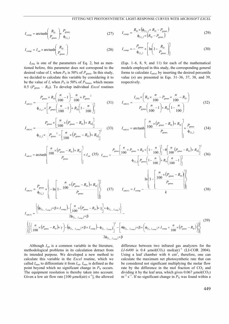
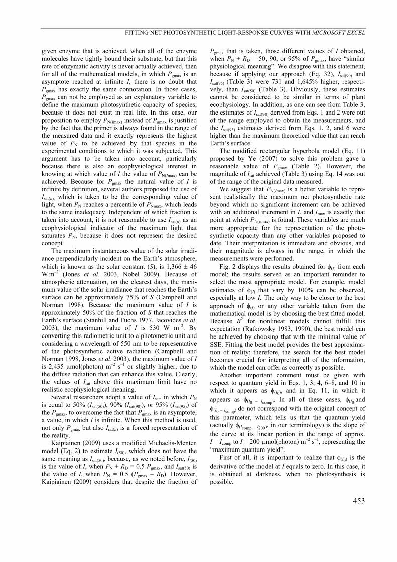
In this study of V. divergens, the mathematical model, which fitted the best the original data of PN/I curve, was the nonrectangular hyperbola (Eq. 6). This model was chosen because it had the lowest SSE (Fig. 1F). All of the regression parameters of the models employed are presented in Table 2.

Models based on the same principle are quite similar and in dependence on the original data they can provide solutions with high or low equality, and even precisely the same value. In this case, one could see that Eqs. 1 and 2, based on the Michaelis-Menten model (Fig. 1A,B), Eqs. 4 and 5, based on a hyperbolic tangent model (Fig. 1D,E), and Eqs. 8 and 9, based on an exponential model

Fig. 1. Fitting PN/I curves by applying different mathematical models for V. diver-gens. The models represented by the Eqs. 1–6, 8, 9, and 11 are represented by the regression lines in A–F, G, H, and I, respectively. PN – net photosynthetic rate; I – photosynthetic photon flux density.


452

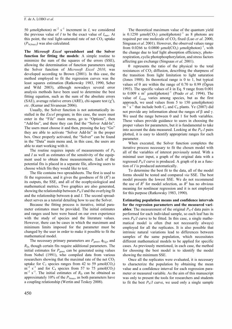
Table 2. The parameters of the regression models employed to fit the net photosynthetic light response curves of V. divergens. Icomp – light compensation point [µmol(photon) m–2 s–1]; Isat – light saturation point [µmol(photon) m–2 s–1]; I(50) – light saturation point for PN + RD equal to 50% of PNmax [µmol(photon) m–2 s–1]; k – adjusting factor [s m2 µmol(photon)–1]; Pgmax – maximum gross photosynthetic rate [µmol(CO2) m–2 s–1]; RD – dark respiration [µmol(CO2) m–2 s–1]; – adjusting factor (dimensionless); – adjusting factor (dimensionless); – convexity factor (dimensionless); ϕ(I0) – quantum yield at I = 0 µmol(photon) m–2 s–1 [µmol(CO2) µmol(photon)–1]; ϕ(I0 – Icomp) – quantum yield at the range between I = 0 µmol(photon) m–2 s–1 and Icomp [µmol(CO2) µmol(photon)–1].

Parameters Mathematical models Eq. 1 Eq. 2 Eq. 3 Eq. 4 Eq. 5 Eq. 6 Eq. 8 Eq. 9 Eq. 11

Pgmax 19.5 19.5 16.4 15.5 15.5 18.4 16.2 15.6

)( oI 0.0899 0.0493 0.0433 0.0709 0.0597

ϕ(I0 – Icomp) 0.0756 RD 1.8 1.8 1.1 0.9 0.9 1.6 1.3 0.6 Isat 359.2 I(50) 216.4 0.4325 K 0.0037 Icomp 10.5 22.6 4.3E–5 0.0039

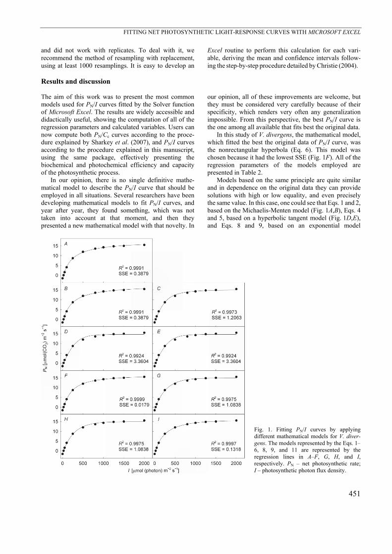
Table 3. The variables calculated from the models. Icomp – light compensation point [µmol(photon) m–2 s–1]; Imax – light saturation point beyond which there is no significant change in PN [µmol(photon) m–2 s–1]; Isat – light saturation point [µmol(photon) m–2 s–1]; Isat(50) – light saturation point for PN + RD equal to 50% of PNmax [µmol(photon) m–2 s–1]; Isat(85) – light saturation point for PN + RD equal to 85% of PNmax [µmol(photon) m–2 s–1]; Isat(90) – light saturation point for A + RD equal to 90% of PNmax [µmol(photon) m–2 s–1]; Isat(95) light saturation point for PN + RD equal to 95% of PNmax [µmol(photon) m–2 s–1]; Pgmax – maximum gross photosynthetic rate [µmol(CO2) m–2 s–1]; PN(Imax) – maximum net photosynthetic rate obtained at I = Imax [µmol(CO2) m–2 s–1]; RD – dark respiration [µmol(CO2) m–2 s–1]; ϕ(Icomp) – quantum yield at I = Icomp [µmol(CO2) µmol(photon)–1]; ϕ(Icomp – I200) – quantum yield at the range between Icomp and I = 200 µmol(photon) m–2 s–1 [µmol(CO2) µmol(photon)–1]; ϕ(I0) – quantum yield at I = 0 µmol(photon) m–2 s–1

[µmol(CO2) µmol(photon)–1]; ϕ(I0 – Icomp) – quantum yield at the range between I = 0 µmol(photon) m–2 s–1 and Icomp [mol(CO2) µmol(photon)–1]. *Photosynthetic active radiation values above the range employed to make the measurements. **Photosynthetic active radiation values above the maximum that reaches the Earth’s surface.

Calculated variables

Mathematical models Eq. 1 Eq. 2 Eq. 3 Eq. 4 Eq. 5 Eq. 6 Eq. 8 Eq. 9 Eq. 11

Icomp 22.5 22.5 22.7 20.2 20.2 23.4 22.0 Isat(50) 261.4 261.4 209.4 211.0 211.0 235.6 210.1 187.6 211.1 Isat(85) 1,376.3 1,376.3 559.2 462.4 462.4 1,022.7 537.0 468.1 678.0 Isat(90) 2,172.6* 2,172.6* 713.1 539.8 539.8 1,564.3 647.0 549.4 854.6 Isat(95) 4,561.7** 4,561.7** 1,047.6 668.7 668.7 3,179.1** 835.2 665.9 1,148.4Isat 2,289.9*

Imax 1537.0 1,949.0 1,030.0 847.0 847.0 1,348.0 1,008.0 1,008.0 1,297.0Pgmax 17.1 PN(Imax) 15.2 15.7 14.5 14.4 14.4 14.9 14.5 14.5 14.9 RD 1.7 ϕ(I0) 0.0899 0.0433 0.0597 0.0824 ϕ(Icomp) 0.0738 0.0738 0.0490 0.0431 0.0431 0.0638 0.0550 0.0574 0.0694 ϕ(I0 – Icomp) 0.0816 0.0816 0.0492 0.0432 0.0432 0.0674 0.0573 0.0586 0.0757 ϕ(Icomp – I200) 0.0410 0.0410 0.0416 0.0391 0.0391 0.0421 0.0400 0.0410 0.0409

(Fig. 1G,H) provided quite similar or even identical results; therefore, they had almost the same values for their regression parameters (Table 2), and the variables calculated from those models were approximately of the

same magnitude (Table 3). There is a difference between what is expected from

the maximum theoretical velocity (Vmax) for an enzyme and Pgmax. If we remember that Vmax is a constant for a


453

given enzyme that is achieved, when all of the enzyme molecules have tightly bound their substrate, but that this rate of enzymatic activity is never actually achieved, then for all of the mathematical models, in which Pgmax is an asymptote reached at infinite I, there is no doubt that Pgmax has exactly the same connotation. In those cases, Pgmax can not be employed as an explanatory variable to define the maximum photosynthetic capacity of species, because it does not exist in real life. In this case, our proposition to employ PN(Imax) instead of Pgmax is justified by the fact that the primer is always found in the range of the measured data and it exactly represents the highest value of PN to be achieved by that species in the experimental conditions to which it was subjected. This argument has to be taken into account, particularly because there is also an ecophysiological interest in knowing at which value of I the value of PN(Imax) can be achieved. Because for Pgmax the natural value of I is infinite by definition, several authors proposed the use of Isat(n), which is taken to be the corresponding value of light, when PN reaches a percentile of PNmax, which leads to the same inadequacy. Independent of which fraction is taken into account, it is not reasonable to use Isat(n) as an ecophysiological indicator of the maximum light that saturates PN, because it does not represent the desired concept.

The maximum instantaneous value of the solar irradi-ance perpendicularly incident on the Earth’s atmosphere, which is known as the solar constant (S), is 1,366 46

W m–2 (Jones et al. 2003, Nobel 2009). Because of atmospheric attenuation, on the clearest days, the maxi-mum value of the solar irradiance that reaches the Earth’s surface can be approximately 75% of S (Campbell and Norman 1998). Because the maximum value of I is approximately 50% of the fraction of S that reaches the Earth’s surface (Stanhill and Fuchs 1977, Jacovides et al. 2003), the maximum value of I is 530 W m–2. By converting this radiometric unit to a photometric unit and considering a wavelength of 550 nm to be representative of the photosynthetic active radiation (Campbell and Norman 1998, Jones et al. 2003), the maximum value of I is 2,435 µmol(photon) m–2 s–1 or slightly higher, due to the diffuse radiation that can enhance this value. Clearly, the values of Isat above this maximum limit have no realistic ecophysiological meaning.

Several researchers adopt a value of Isat, in which PN is equal to 50% (Isat(50)), 90% (Isat(90)), or 95% (Isat(95)) of the Pgmax, to overcome the fact that Pgmax is an asymptote, a value, in which I is infinite. When this method is used, not only Pgmax but also Isat(n) is a forced representation of the reality.

Kaipiainen (2009) uses a modified Michaelis-Menten model (Eq. 2) to estimate I(50), which does not have the same meaning as Isat(50), because, as we noted before, I(50) is the value of I, when PN + RD = 0.5 Pgmax, and Isat(50) is the value of I, when PN = 0.5 (Pgmax – RD). However, Kaipiainen (2009) considers that despite the fraction of

Pgmax that is taken, those different values of I obtained, when PN + RD = 50, 90, or 95% of Pgmax, have “similar physiological meaning”. We disagree with this statement, because if applying our approach (Eq. 32), Isat(90) and Isat(95) (Table 3) were 731 and 1,645% higher, respecti-vely, than Isat(50) (Table 3). Obviously, these estimates cannot be considered to be similar in terms of plant ecophysiology. In addition, as one can see from Table 3, the estimates of Isat(90) derived from Eqs. 1 and 2 were out of the range employed to obtain the measurements, and the Isat(95) estimates derived from Eqs. 1, 2, and 6 were higher than the maximum theoretical value that can reach Earth’s surface.

The modified rectangular hyperbola model (Eq. 11) proposed by Ye (2007) to solve this problem gave a reasonable value of Pgmax (Table 2). However, the magnitude of Isat achieved (Table 3) using Eq. 14 was out of the range of the original data measured.

We suggest that PN(Imax) is a better variable to repre-sent realistically the maximum net photosynthetic rate beyond which no significant increment can be achieved with an additional increment in I, and Imax is exactly that point at which PN(Imax) is found. These variables are much more appropriate for the representation of the photo-synthetic capacity than any other variables proposed to date. Their interpretation is immediate and obvious, and their magnitude is always in the range, in which the measurements were performed.

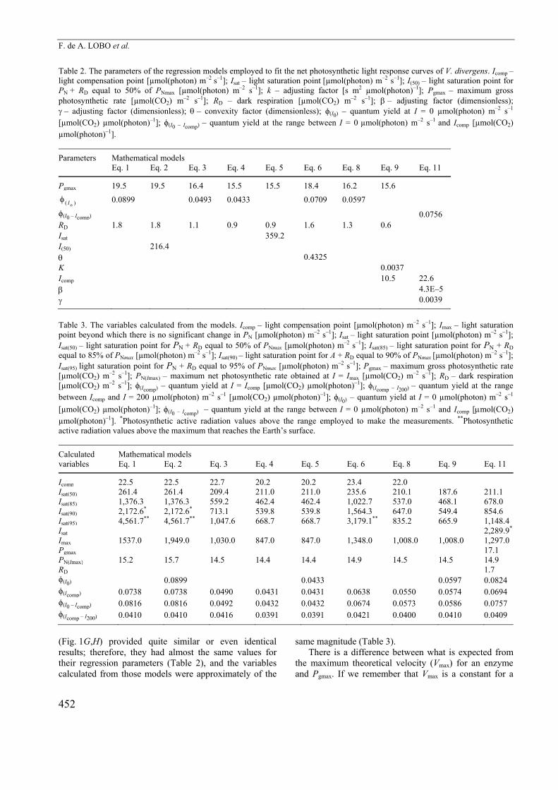
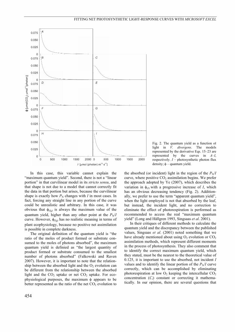
Fig. 2 displays the results obtained for (I) from each model; the results served as an important reminder to select the most appropriate model. For example, model estimates of (I) that vary by 100% can be observed, especially at low I. The only way to be closer to the best approach of (I) or any other variable taken from the mathematical model is by choosing the best fitted model. Because R2 for nonlinear models cannot fulfill this expectation (Ratkowsky 1983, 1990), the best model can be achieved by choosing that with the minimal value of SSE. Fitting the best model provides the best approxima-tion of reality; therefore, the search for the best model becomes crucial for interpreting all of the information, which the model can offer as correctly as possible.

Another important comment must be given with respect to quantum yield in Eqs. 1, 3, 4, 6–8, and 10 in which it appears as ϕ(I0), and in Eq. 11, in which it appears as ϕ(I0 – Icomp). In all of these cases, ϕ(I0)and ϕ(I0 – Icomp) do not correspond with the original concept of this parameter, which tells us that the quantum yield (actually ϕ(Icomp – I200), in our terminology) is the slope of the curve at its linear portion in the range of approx. I = Icomp to I = 200 µmol(photon) m–2 s–1, representing the “maximum quantum yield”.

First of all, it is important to realize that ϕ(I0) is the derivative of the model at I equals to zero. In this case, it is obtained at darkness, when no photosynthesis is possible.


454

Fig. 2. The quantum yield as a function of light in V. divergens. The models represented by the derivative Eqs. 15–23 are represented by the curves in A–I, respectively. I – photosynthetic photon flux density; – quantum yield.

In this case, this variable cannot explain the

“maximum quantum yield”. Second, there is not a “linear portion” in that curvilinear model in its stricto sensu, and that shape is not due to a model that cannot correctly fit the data in that portion but arises, because the curvilinear shape is exactly how PN changes with I in most cases. In fact, forcing any straight line in any portion of the curve could be unrealistic and arbitrary. In this case, it was obvious that ϕ(I0) is always the maximum value of the quantum yield, higher than any other point at the PN/I curve. However, ϕ(I0) has no realistic meaning in terms of plant ecophysiology, because no positive net assimilation is possible in complete darkness.

The original definition of the quantum yield is “the ratio of the moles of product formed or substrate con-sumed to the moles of photons absorbed”, the maximum quantum yield is definied as “the largest quantity of product formed or substrate consumed to the smallest number of photons absorbed” (Falkowski and Raven 2007). However, it is important to note that the relation-ship between the absorbed light and the O2 evolution can be different from the relationship between the absorbed light and the CO2 uptake or net CO2 uptake. For eco-physiological purposes, the maximum appears to be better represented as the ratio of the net CO2 evolution to

the absorbed (or incident) light in the region of the PN/I curve, where positive CO2 assimilation begins. We prefer the approach adopted by Ye (2007), which describes the variation in (I)with a progressive increase of I, which has an obvious decreasing tendency (Fig. 2). Addition-ally, we prefer to use the term “apparent quantum yield”, when the light employed is not that absorbed by the leaf, but instead, the incident light, and no correction to eliminate the effect of photorespiration is performed as recommended to access the real “maximum quantum yield” (Long and Hällgren 1993, Singsaas et al. 2001).

In their critiques of different methods to calculate the quantum yield and the discrepancy between the published values, Singsaas et al. (2001) noted something that we have already mentioned about using O2 evolution or CO2 assimilation methods, which represent different moments in the process of photosynthesis. They also comment that to identify the correct maximum quantum yield, which they stated, must be the nearest to the theoretical value of 0.125, it is important to use the absorbed, not incident I values and to identify the linear portion of the PN/I curve correctly, which can be accomplished by eliminating photorespiration at low O2 keeping the intercellular CO2 concentration (Ci) constant or correcting it mathema-tically. In our opinion, there are several questions that


455

must be considered in this context. As we stated in the previous paragraph, the most common shape of the PN/I curve is curvilinear throughout its length, thus, no linear phase is clearly identifiable. However, if the shape is very close to linear, the method that Singsaas et al. (2001) employed to determine how much of the data could be included in that phase is inappropriate. As mentioned by Dubois et al. (2007), the upward progression in the coefficient of determination (R2) with the withdrawal of observations is inherent to its definition, thus, this parameter cannot be used as a criterion to choose data to be included or excluded from the estimation. Depending on the focus, in terms of ecophysiological research, it appears to be much more reasonable to use one theoretical maximum quantum yield (max = 0.125) as the reference to identify how stress factors or specific treatments applied to the plant can affect quantum yield or any other PN/I parameter or calculated variable.

For us, the approach of Ye (2007) to calculation of (I)

produces a result that is much more realistic and useful, because one can observe how the variable can change with I, and particularly for ecophysiological purposes, all of those points in the curve can be analyzed, when PN is above the light compensation point, which means that a net CO2 uptake is taking place. The variables ϕ(I0),

ϕ(I0 – Icomp), and ϕ(Icomp) all fail in representing the maxi-mum value of the quantum yield, because they are defined below or at the light compensation point. ϕ(Icomp – I200) is also problematic in fixing the point at which the calculation of the quantum yield must be performed, and depending on the species. Thus, this value may not be reasonable.

By applying the approach of Ye (2007), the values of quantum yieldcan be analyzed not only, when PN is dependent on I, but also when PN becomes progressively independent of I. This capability is very useful for evaluating differences in the photosynthetic efficiency between sun and shade leaves, for which, not always but frequently, no difference in can be observed in the initial portion of the PN/I curve.

In conclusion, we consider that our Excel routines are an interesting alternative for users with any level of statistical knowledge to evaluate and quickly identify the best model of PN/I curve that fits better their experimental data. We also consider that the variables, which better represent the light-saturated rate of CO2 uptake, the light saturation point, and the quantum yield are PN(Imax), Imax, and (I), respectively.

References Abe, M., Yokota, K., Kurashima, A., Maegawa, M.: High water

temperature tolerance in photosynthetic activity of Zostera japonica Ascherson and Graebner seedlings from Ago Bay, Mio Prefecture, central Japan. – Fish. Sci. 75: 1117-1123, 2009.

Baly, E.C.C.: The kinetics of photosynthesis. – Proc. R. Soc. Lond. B 117: 218-239, 1935.

Brown, A.M.: A step-by-step guide to non-linear regression analysis of experimental data using a Microsoft Excel spreadsheet. – Comput. Methods Programs Biomed. 65: 191-200, 2001.

Campbell, G.S., Norman, J.M.: An Introduction to Environ-mental Biophysics. 2nd Ed. Springer-Verlag, New York 1998.

Chen, L., Tam, N.F.Y., Huang, J. et al.: Comparison of ecophysiological characteristics between introduced and indigenous mangrove species in China. – Est. Coast Shelf Sci. 79: 644-652, 2008.

Christie, D.: Resampling with Excel. – Teach. Stat. 26: 9-13, 2004.

Devacht, S., Lootens, P., Roldán-Ruiz, I. et al.: Influence of low temperatures on the growth and photosynthetic activity of industrial chicory, Cichorium intybus L. partim. – Photosynthetica 47: 372-380, 2009.

Donovan, T.M., Welden, C.W.: Spreadsheet Exercises in Ecology and Evolution. Sinauer Associates, Sunderland 2002.

Dubois, J.-J.B., Fiscus, E.L., Booker, F.L. et al.: Optimizing the statistical estimation of the parameters of the Farquhar-Von Caemmerer-Berry model of photosynthesis. – New Phytol. 176: 402-414, 2007.

Falkowski, P.G., Raven, J.A.: Aquatic Photosynthesis.

Princeton University Press, Princenton 2007. Gallegos, C.L., Platt, T.: Photosynthesis measurements on

natural populations of phytoplankton: numerical analysis. – Can. Bull. Fish. Aquat. Sci. 210: 103–112, 1981.

Govindjee, Beatty, J.T., Gest, H., Allen, J.F.: Discoveries in Photosynthesis. Springer, Dordrecht 2005.

Harley, P.C., Baldocchi, D.D.: Scaling carbon dioxide and water vapor exchange from leaf to canopy in a deciduous forest. I. Leaf model and parametrization. – Plant Cell Environ. 18: 1146-1156, 1995.

Hunt, R., Causton, D.R., Shipley, B., Askew, A.P.: A modern tool for classical growth analysis. – Ann. Bot. 90: 485-488, 2002.

Jacovides, C.P., Tymvios, F.S., Asimakopoulos, D.N. et al.: Global photosynthetically active radiation and its relationship with global solar radiation in the Eastern Mediterranean basin. – Theor. Appl. Climatol. 74: 227-233, 2003.

Jassby, A.D., Platt, T.: Mathematical formulation of the relationship between photosynthesis and light for phytoplankton. – Limnol. Oceanogr. 21: 540-547, 1976.

Jones, H.B., Archer, N., Rotenberg, E., Casa, R.: Radiation measurement for plant ecophysiology. – J. Exp. Bot. 54: 879-889, 2003.

Jones, M.B.: Photosynthetic responses of C3 and C4 wetland species in a tropical swamp. – J. Ecol. 76: 253-262, 1988.

Kaipiainen, E.L.: Parameters of photosynthesis light curve in Salix dasyclados and their changes during the growth season. – Russ. J. Plant Physiol. 56: 445-453, 2009.

Kok, B.: On the interrelation of respiration and photosynthesis in green plants. – Biochim. Biophys. Acta 3: 625-631, 1949.


456

Kumar, K.V., Sivanesan, S.: Isotherm parameters for basic dyes onto activated carbon: comparison of linear and non-linear method. – J. Hazard. Mater. 129: 147-150, 2006.

Lambers, H., Chapin III, F.S., Pons, T.L.: Response of photosynthesis to light. – In: Lambers, H., Chapin III, F.S., Pons, T.L. (eds.): Plant Physiological Ecology. Pp. 26-47. Springer, New York 2008.

LI-COR Bioscience: Using the LI-6400 Version 5. LI-COR Bioscience, Inc., Lincoln, NE, USA 2004.

Lloyd, J., Grace, C., Miranda, A.C. et al.: A simple calibrated model of Amazon rainforest productivity based on leaf biochemical properties. – Plant Cell. Environ. 18: 1129-1145, 1995.

Long, S.P., Hällgren, J.-E.: Measurement of CO2 assimilation by plants in the field and the laboratory. – In: Hall, D.O., Scurlock, J.M.O., Bolhàr-Nordenkampf, H.R. et al. (eds.): Photosynthesis and Production in a Changing Environment. A Field and Laboratory Manual. Pp. 129-167. Chapman and Hall, London 1993.

Lootens, P., Van Waes, J., Carlier, L.: Effect of a short photo-inhibition stress on photosynthesis, chlorophyll a fluorescence and pigment contents of different maize cultivars. Can a rapid and objective stress indicator be found? – Photosynthetica 42: 187-192, 2004.

Luo, Y., Hui, D., Cheng, W. et al.: Canopy quantum yield in a mesocosm study. – Agric. For. Meteorol. 100: 35-48, 2000.

Nobel, P.S.: Physicochemical and Environmental Plant Physiology. Elsevier, Amsterdam 2009.

Nobel, P.S.: Achievable productivities of certain CAM plants: basis for high values compared with C3 and C4 plants. – New Phytol. 119: 183-205, 1991.

Ögren, E.: Convexity of the photosynthetic light-response curve in relation to intensity and direction of light during growth. – Plant Physiol. 101: 1013-1019, 1993.

Prado, C.H.B.A., de Moraes, J.P.A.P.V., de Mattos, E.A.: Gas exchange and leaf water status in potted plants of Copaifera langsdorffii. 1. Responses to water stress. – Photosynthetica 30: 207-213, 1994.

Prado, C.H.B.A., de Moraes, J.P.A.P.V.: Photosynthetic capa-city and specific leaf mass in twenty woody species of cerrado vegetation under field conditions. – Photosynthetica 33: 103-

112, 1997. Prioul, J.L., Chartier, P.: Partitioning of transfer and carboxy-

lation components of intracellular resistance to photosynthetic CO2 fixation: A critical analysis of the methods used. – Ann. Bot. 41: 789-800, 1977.

Ratkowsky, D.A.: Nonlinear Regression Modeling – A Unified Practical Approach. Marcel Dekker, New York 1983.

Ratkowsky, D.A.: Handbook of Nonlinear Regression Models. Marcel Dekker, New York 1990.

Seber, G.A.F., Wild, C.J.: Nonlinear Regression. Wiley-Interscience, Hoboken 2003.

Sharkey, T.D., Bernacchi, C.J., Farquhar, G.D., Singsaas, E.L.: In Practice: Fitting photosynthetic carbon dioxide response curves for C3 leaves. – Plant Cell Environ. 30: 1035-1040, 2007.

Singsaas, E.L., Ort, D.R., DeLucia, E.H.: Variation in measured values of photosynthetic quantum yield in ecophysiological studies. – Oecologia 128: 15-23, 2001.

Smith, E.L.: Photosynthesis in relation to light and carbon dioxide. – PNAS 22: 504-511, 1936.

Stanhill, G., Fuchs, M.: The relative flux density of photo-synthetically active radiation. – J. Appl. Ecol. 14: 317-322, 1977.

Vervuren, P.J.A., Beurskens, M.H.H., Blom, C.W.P.M.: Light acclimation, CO2 response and long-term capacity of underwater photosynthesis in three terrestrial plant species. – Plant Cell Environ. 22: 959-968, 1999.

Webb, W.L., Newton, M., Starr, D.: Carbon dioxide exchange of Alnus rubra: a mathematical model. – Oecologia 17: 281-291, 1974.

Wertin, T.M., Teskey, R.O.: Close coupling of whole-plant respiration to net photosynthesis and carbohydrates. – Tree Physiol. 28: 1831-1840, 2008.

Ye, Z.-P.: A new model for relationship between irradiance and the rate of photosynthesis in Oryza sativa. – Photosynthetica 45: 637-640, 2007.

Zeinalov, Y.: Mechanisms of photosynthetic oxygen evolution and fundamental hypotheses of photosynthesis. – In: Pessarakli, M. (ed.): Handbook of Photosynthesis. Pp. 3-19. Taylor and Francis, Boca Ratón 2005.

fitting net photosynthetic light-response curves with ... · fitting net photosynthetic...

Documents