five effects of mantle dynamics
TRANSCRIPT

CHAPTER FIVE
Effects of mantle dynamics
Summary
Plate tectonics operates in the upper thermal boundary layer of an underlying mantle convection system. Flow within the mantle takes place
at different spatial scales, including flows induced by the subduction of cold lithospheric slabs, incubation under continental lids, small-scale
convection driven by edge effects, lower-mantle megaplumes, and upper-mantle hotspots. This flow and the consequent mass anomalies at
depth result in a dynamic topography at the Earth’s surface that is important in basin analysis.
The starting point for an analysis of mantle flow is a consideration of buoyancy forces set up by density heterogeneities in the mantle.
Buoyancy forces are counteracted by viscous resistance. The force balance provides fundamental information about the scaling between
parameters and allows the derivation of dimensionless groups that describe various aspects of the flow and thermal characteristics of a fluid
layer, such as the Rayleigh number. Consideration of the Rayleigh number for the mantle indicates that convection must be occurring. This
convective flow efficiently transports heat and drives high plate velocities, but is laminar.
Numerical and physical experiments illustrate the convection patterns of upwellings and downwellings produced by heating a fluid layer
from below, from the surface and with internal radiogenic heating. Models using highly temperature-dependent viscosity structures in the
mantle suggest that large aspect ratio convection cells are stable, such as must underlie the Pacific plate. Detailed three-dimensional velocity
models of the mantle (seismic tomography) also show mass anomalies that must be sustained by flow. These mass anomalies show that the
effects of plate tectonics, such as mid-ocean ridges and subducting slabs, can be recognised deep into the Earth’s interior.
Measurements of the Earth’s gravity field reveal geoid height anomalies. An underlying convecting system should produce variations in the
height of the geoid over upwelling and downwelling limbs. At long wavelength, the observed geoid of the Earth shows major zones of positive
and negative geoid anomaly. Viscous flow models of the mantle suggest that mass excesses in the upper mantle caused by the remnants of cold
subducted slabs generate geoid lows, whereas hotspots and mid-ocean ridges are correlated with the presence of hot megaplumes in the lower
mantle and are associated with geoid highs.
The surface topography on land, and the bathymetry beneath the sea, produced by mantle flow, is known as dynamic topography. It repre-
sents a deflection of the surface of the Earth caused by the presence of ‘blobs’ of buoyancy in the mantle. It can be recognised, for example,
in regions of plate subduction due to the cooling effect of the oceanic slab, beneath supercontinents due to heating caused by the presence of
an insulating lid, near the edges of continents due to small-scale convection triggered by the ocean–continent boundary, and, of course, in the
form of topographic ‘hotspot’ swells in the ocean associated with magmatism. Some of the sub-plate flow structures responsible for topographic
doming and magmatism are thought to be plumes originating from the core–mantle boundary. There is evidence of unsteadiness in plume
activity, with pulses of buoyancy causing relatively rapid uplift of the Earth’s surface followed by subsidence. Such pulses may cause cycles of
erosional landscape development and delivery of sands to the deep sea, followed by draping with marine sediments.
Mantle flow is commonly associated with melt generation, igneous underplating and surface magmatism. The presence of plumes may cause
sufficient elevation of asthenospheric temperatures to result in adiabatic decompression and the formation of flood basalt provinces (large
igneous provinces – LIPs). The North Atlantic igneous province and the Ethiopian Afar regions are examples. LIPs are commonly connected
to currently active volcanic hotspots by tracks of extinct volcanoes.
Mantle dynamics affects basin development by causing topographic uplift and the export of particulate sediment from erosional landscapes
to sedimentary basins. Mantle dynamics also causes negative dynamic topography in the form of sag-type basins of the continental interiors.
In geological history, cratonic basins have initiated preferentially at times of continental dispersal away from supercontinental assemblies. Their
long, slow subsidence has been attributed to negative dynamic topography over cold downwellings, to thermal contraction of previously
stretched and heated thick continental lithosphere, and to sediment loading following an earlier stage of stretching.
Dynamic uplift of the continental surface produces domal features that promote centrifugal river drainage patterns. The periods of dynamic
uplift can potentially be recognised by the location of erosive knickzones in the river long profile. Time-varying dynamic topography may also
affect the position of continental drainage divides and the direction of river discharge to the ocean, as in the reversal of Amazon drainage from
the Pacific to the Atlantic.
Dynamic topography is also a primary factor in the history of long-term sea-level change and the extent of continental flooding. In particular,
times of extensive uplift of the seafloor in the form of superswells, as in the Pacific during the Cretaceous, may be primarily responsible for
elevated sea levels, rather than reflecting increases in spreading rate in the mid-ocean ridge system.
Basin Analysis: Principles and Application to Petroleum Play Assessment, Third Edition. Philip A. Allen and John R. Allen.© 2013 John Wiley & Sons, Ltd. Published 2013 by John Wiley & Sons, Ltd.

154 Effects of mantle dynamics
ture (and/or chemical) heterogeneities. These heterogeneities reveal
a picture of deep penetration of cold subducted lithospheric slabs
into the mantle, and of large hot upwellings that seem to rise from a
highly dynamic core–mantle boundary (Fig. 5.1). Subducted slabs of
lithosphere appear to both penetrate and to queue at the 670 km
discontinuity. The residues of the subducted slabs that penetrate the
discontinuity appear to descend to the core–mantle boundary, where
they are reheated before being resurrected as a mantle plume. Mantle
plumes appear to travel upwards and impinge on the base of the
lithosphere, spreading out like a mushroom, and uplifting the overly-
ing plate. Extension of the lithosphere over the plume head may lead
to continental splitting (Chapter 3), the formation of new spreading
centres and further subduction of lithosphere.
Convection systems in the mantle are the engines for the surface
tangential motions of plates. Subducting slabs are cold downwellings,
and spreading oceanic ridges are upwellings (Davies & Richards
1992), so the lithospheric plates must be regarded as an integral part
of the convection system rather than being dragged passively by basal
traction over the convection system. In other words, plate tectonics
is the surface expression of convection.
Plate tectonic theory explains a wide range of geological and geo-
physical observations in the oceans and at plate boundaries. It has
been far less successful in explaining the topography, seismicity, neo-
5.1 Fundamentals and observations
5.1.1 Introduction: mantle dynamics and plate tectonics
Although plate tectonics has been highly successful as an explanation
of the relative motion of plates and the deformation at their bounda-
ries, there is little integration of mantle dynamics into what is essen-
tially a kinematic theory. For example, volcanic hotspots such as
those of Hawaii and Iceland, which are related to the ascent of deeply
rooted mantle plumes, do not fit into plate tectonic theory. Within
the solar system, the operation of plate tectonics is unique to Earth,
but plume volcanism occurs on Mars and Venus as well as on a
number of moons. The surface of Mars appears to be a single static
plate acting as a ‘frozen lid’; Venus is a convecting planet beneath a
thick viscous lid, but no mobile plates, and the tectonics is spatially
continuous and unstable. On Earth, therefore, we have a particular
problem in understanding the interaction of internal thermal con-
vection with an upper thermal boundary layer made of a discrete
number of plates in relative motion.
The three-dimensional mapping of seismic velocity variations
in the mantle (seismic tomography) now provides unprecedented
detail on small but systematic density variations that reflect tempera-
Fig. 5.1 Schematic section through a segment of the Earth showing the subduction of lithospheric slabs that are laid out along the 670 km discontinuity or penetrate to a graveyard above the core–mantle boundary (CMB). A mantle plume is shown rising from the CMB to produce a hotspot in the overlying oceanic plate. Modified from Stern (2002) and reproduced with permission of John Wiley & Sons, Inc.
370 km
670 km
2885 km
5144 km
6371 km
Lower mantle
(Mesosphere)
Outer core
(liquid)
Inner core
(solid)
Spreading
ridge Hotspot
Arc volcano
Asthenosphere
Transition zone
Arc-trench
complex
Mantle plume
CMB
Continental
crust
Oceanic
crust
Core

Effects of mantle dynamics 155
where D is the depth of the vertically descending slab, and ρ, µ, κ
and T are the density, viscosity, thermal diffusivity and temperature
of the interior of the fluid mantle (Fig. 5.2). Using parameter values
of D = 3000 km (thickness of the whole mantle), ρ = 4000 kg m−3,
T = 1400 °C, µ = 1022 Pa s, α = 2 × 10⁻⁵ °C−1 and κ = 10−6 m2 s−1, the
downward velocity is 90 mm yr−1. This is close to the known velocities
of plate motion (Lithgow-Bertelloni & Richards 1998).
The same force balance allows the thickness of the lithosphere at
the point of subduction d to be estimated, treating it as a diffusive
length scale (see §2.2.7) equal to κt (or κ D u/ ), and the surface
heat flux to be estimated, using Fourier’s law (see §2.2.2), which states
q = KT/d where K is the thermal conductivity. Using the same param-
eter values as above, and K = 3 W m−1 K−1, we obtain 33 km for the
thickness of the oceanic lithosphere and 130 mW m−2 for the surface
oceanic heat flow. These values are consistent with observations of
oceanic plates, suggesting that a basic theory of mantle flow driven
by buoyancy explains at first order the velocities of plates.
Combining eqn. [5.2] and the expression for diffusion length
(d t= κ ) gives an expression with two dimensionless groups that
embeds how the different parameters scale:
D
d
g TD
=
3 3
4
ρακµ
[5.3]
For example, eqn. [5.3] can be used to ask ‘what would be the
lithospheric thickness, heat flow and plate velocity if the mantle
viscosity were 10 times lower at some early stage in the evolution
of the Earth’? Keeping other parameter values constant, the plate
thickness would reduce to 15 km, the heat flow would increase to
275 mW m−2, and the plate velocity would increase to c.400 mm yr−1.
tectonics and subsidence history of the continental interiors. This is
partly due to the complex rheology of the continental lithosphere,
and partly due to the lack of integration of mantle dynamics into a
satisfactory explanation of continental deformation and basin devel-
opment. Stratigraphers have long recognised the supreme impor-
tance of vertical movements (‘epeirogeny’) of the continents in
generating the stratigraphic sequences of the world’s cratons (Sloss
1963). In particular, the major transgressions of the continents that
have taken place through geological time (e.g. Cambrian–Early
Ordovician and Late Cretaceous, Bond 1979) cannot be explained
purely by a eustatic sea-level rise (Bond 1976, 1978) and must involve
a major component of widespread relative sea-level rise most likely
related to mantle processes (§5.4.3).
It is increasingly recognised, therefore, that the near-surface
motion of lithospheric plates needs to be understood by reference to
the mantle convection system (Anderson 1982). In Chapter 5, we
look briefly at the evidence for flow in the mantle, with the specific
goal of understanding the significance of this flow for subsidence
within continental sedimentary basins. The reader is referred to
§2.2.8 for introductory material on mantle viscosity, convection in
the mantle and the adiabatic temperature gradient. The rheology of
mantle rocks is dealt with in §2.3.2.
5.1.2 Buoyancy and scaling relationships: introductory theory
The buoyancy contrasts of the interior of the Earth, which are the
forces responsible for its flow, derive essentially from lateral (hori-
zontal) density contrasts. These density contrasts may be thermal or
compositional in origin.
Buoyancy results from gravity acting on a density contrast Δρ in
a volume V. It is a force B given by
B gV g m= − = −∆ ∆ρ [5.1]
where Δm is the mass anomaly resulting from the density contrast
and the minus sign is because gravity and weight are positive down-
wards whereas buoyancy is conventionally positive upwards (Davies
1999, p. 212). Consequently, the buoyancy force depends strongly
on the volume of the density contrast. The density contrast resulting
from temperature differences is given by the volumetric coefficient
of thermal expansion αv (eqn. [2.12]). Using parameter values for
mantle rock, a temperature difference of 1000 °C causes just a 3%
change in density. Nevertheless, large buoyancy forces in the mantle
may result from the subduction of cold slabs of lithosphere
(negative buoyancy) or from the presence of plume heads (positive
buoyancy).
A simple consideration of the buoyancy forces associated with the
motion of plates explains convection in the mantle (Turcotte &
Oxburgh 1967) (see §5.1.3). A plate represents a cooled thermal
boundary layer, so is cold and tends to sink due to negative buoyancy.
The sinking is opposed by viscous stresses caused by the resulting
flow of the mantle, with the stresses increasing with the velocity of
the sinking. Consequently, a balance is reached between the viscous
resistance and the negative buoyancy at a certain velocity u, given by
Davies (1999, p. 216)
u Dg Tv
=
ρα κµ4
2 3
[5.2]
Fig. 5.2 Sketch (a) and model set-up (b) of a convective flow driven by subduction at velocity v of a plate thickness d in a fluid layer of thickness D, viscosity µ and temperature T. After Davies (1999, p. 214), © Cambridge University Press, 1999.
v
v
v
v
Temperature T
Viscosity µ
Velocity v
Diffusivity κ
D
D d
d
T = 0
T = 0
v
d
TD
(a)
(b)

156 Effects of mantle dynamics
number is a measure of turbulence. For the mantle, Ra ≈ 3 × 10⁶,
Pe ≈ 9000, Nu ≈ 100, and Re ≈ 10−18, indicating a strongly convect-
ing layer driving high plate velocities and vigorous heat loss, but
laminar flow.
5.1.3 Flow patterns in the mantle
The standard starting point for studies of convection is a layer of fluid
heated from below and cooled at the top (Fig. 5.3a). Fluid close to
the cold upper surface is cooled, forming a cold thermal boundary
layer that is the lithosphere or plate. Likewise, fluid close to the hot
lower surface is heated, forming a hot thermal boundary layer. Above
a critical Rayleigh number, hot material rises from the lower bound-
ary layer and reinforces the downward motion of fluid from the
upper boundary layer, forming a series of rotating cells. The convec-
tion cells have a width that scales on the thickness of the fluid layer
(Bercovici et al. 2000).
Differences in the flow patterns are expected depending on the
precise conditions at the lower and upper boundaries and within the
fluid layer itself. For example, if the fluid layer is self-heated by radio-
genic heat production, and the lower boundary is insulating (involv-
ing no heat flow) (Fig. 5.3b), then cold downwellings would originate
from the cooled upper boundary layer, but any upwellings would be
a passive response rather than involving positively buoyant material.
In other words, the fact that upwelling is occurring, as at mid-ocean
ridges, does not mean that the ascending mantle material is hotter
than average. The upwelling material is simply being displaced by the
descending cold mantle material.
The right-hand side of eqn. [5.3] is a dimensionless group that
contains a great deal of information about convection of a fluid layer.
Removing the numerical factor 4, it is the Rayleigh number. The
Rayleigh number is a measure of the likelihood and vigour of convec-
tion. For the parameter values above, the mantle has a Ra of c.3 × 106.
Rewriting eqn. [5.3] it is clear that the length scale of the convection
depends on the Rayleigh number Ra as follows
d
DkRa=
−1 3 [5.4]
where the coefficient of proportionality k is about 1.6. In other words,
if Ra increases, the cooled boundary layer of lithosphere d reduces
in thickness relative to the depth of the convecting layer D. At
Ra = 3 × 10⁶, d is about 1% of the thickness of the convecting layer.
In a similar fashion, other parameter groups can be scaled against
Ra. Instead of investigating length scales, we could choose velocities,
in which case
u
URa~
2 3 [5.5]
where U is the characteristic velocity of the problem equal to κ/D.
This ratio u/U is a Péclet number, which for parameter values typical
of the mantle is approximately 9000.
The heat flow q can also be expressed in terms of its scaling with
the Rayleigh number. Modifying eqn. [5.4] with Fourier’s law gives
qKT
DRa=
1 3 [5.6]
where the scaling variable (KT/D) expresses the heat that would be
conducted across the entire fluid layer in the absence of convection.
The total heat flow (in the presence of convection) q versus the con-
ductive heat flow KT/D is known as the Nusselt number, Nu. Conse-
quently, eqn. [5.6] becomes Nu ∼ Ra1/3. For the mantle, the Nusselt
number is about 100, indicating that heat flow by convection is two
orders of magnitude more efficient than that by conduction.
Accepting that the mantle is convecting in some way, it is possible
to estimate whether the flow is laminar or turbulent. This is given by
the Reynolds number Re
Re =
ud
ν
[5.7]
where u is the velocity of the flow, d is the length scale and ν is the
kinematic viscosity equal to µ/ρ. The kinematic viscosity of the
mantle is difficult to estimate, since it is dependent on the tempera-
ture, but let us take a value of 1017 m2 s−1 as appropriate for the upper
mantle. The flow velocity can be estimated from flow laws for incom-
pressible Newtonian fluids; let us take uρ = 10−7 m s−1 as an order
of magnitude estimate (1 m yr−1 is 3.17 × 10⁻⁸ m s−1, so u is about
30 mm yr−1 in this calculation). Using eqn. [5.7], Re is c.7 × 10−19. This
is much smaller than the critical Re for turbulence, indicating that
the convecting flow in the mantle is laminar.
In summary, a simple quantitative model of convection involving
a fluid layer with a cooled thermal boundary layer undergoing sub-
duction allows the scaling relationships between parameter groups
to be investigated. The Rayleigh number predicts the onset and
vigour of convection, the Péclet number is a measure of the velocity
of the plate as a cooled thermal boundary layer, the Nusselt number
indicates the efficiency of heat flow by convection, and the Reynolds
Fig. 5.3 Various modes of heating of a fluid layer, with tem-perature profiles. (a) Layer of fluid heated from below and cooled at the top. (b) Insulating (no flux) boundary below and internally self-heated by radiogenic decay. (c) Hot lower boundary and internally heated fluid layer. See text for explanation. After Davies (1999, p. 226) © Cambridge University Press, 1999.
Cold
Hot
Upwelling
Downwelling
Internal heating
Internal heating
Hot
Cold
Cold
Insulating
Temp
Temp
Temp
(a)
(b)
(c)
Lower boundary
Upper boundary
Effects of mantle dynamics 157
The simplest type of convection is two-dimensional, with counter-
rotating cylinders or rolls in the third dimension. The horizontal
dimensions of the individual convecting cells in a fluid layer of verti-
cal thickness D, heated from below, is approximately equal to D.
This horizontal dimension is also the length of the horizontal cur-
rents in the thermal boundary layers. In the simplest terms, the length
of the horizontal currents is determined by the amount of cooling
necessary to induce gravitational instability and downwelling. At a
higher Rayleigh number (Ra ∼ 105) in fluids of constant viscosity, a
three-dimensional pattern develops (Busse & Whitehead 1971),
which may be bimodal or spoke-like, with linear upwellings joining
at a vertex. Fluids with temperature-dependent viscosity produce
three-dimensional polyhedral patterns of squares, triangles and
hexagons.
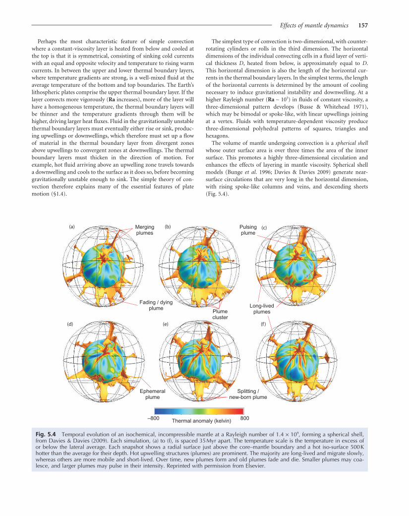
The volume of mantle undergoing convection is a spherical shell
whose outer surface area is over three times the area of the inner
surface. This promotes a highly three-dimensional circulation and
enhances the effects of layering in mantle viscosity. Spherical shell
models (Bunge et al. 1996; Davies & Davies 2009) generate near-
surface circulations that are very long in the horizontal dimension,
with rising spoke-like columns and veins, and descending sheets
(Fig. 5.4).
Perhaps the most characteristic feature of simple convection
where a constant-viscosity layer is heated from below and cooled at
the top is that it is symmetrical, consisting of sinking cold currents
with an equal and opposite velocity and temperature to rising warm
currents. In between the upper and lower thermal boundary layers,
where temperature gradients are strong, is a well-mixed fluid at the
average temperature of the bottom and top boundaries. The Earth’s
lithospheric plates comprise the upper thermal boundary layer. If the
layer convects more vigorously (Ra increases), more of the layer will
have a homogeneous temperature, the thermal boundary layers will
be thinner and the temperature gradients through them will be
higher, driving larger heat fluxes. Fluid in the gravitationally unstable
thermal boundary layers must eventually either rise or sink, produc-
ing upwellings or downwellings, which therefore must set up a flow
of material in the thermal boundary layer from divergent zones
above upwellings to convergent zones at downwellings. The thermal
boundary layers must thicken in the direction of motion. For
example, hot fluid arriving above an upwelling zone travels towards
a downwelling and cools to the surface as it does so, before becoming
gravitationally unstable enough to sink. The simple theory of con-
vection therefore explains many of the essential features of plate
motion (§1.4).
Fig. 5.4 Temporal evolution of an isochemical, incompressible mantle at a Rayleigh number of 1.4 × 10⁹, forming a spherical shell, from Davies & Davies (2009). Each simulation, (a) to (f), is spaced 35 Myr apart. The temperature scale is the temperature in excess of or below the lateral average. Each snapshot shows a radial surface just above the core–mantle boundary and a hot iso-surface 500 K hotter than the average for their depth. Hot upwelling structures (plumes) are prominent. The majority are long-lived and migrate slowly, whereas others are more mobile and short-lived. Over time, new plumes form and old plumes fade and die. Smaller plumes may coa-lesce, and larger plumes may pulse in their intensity. Reprinted with permission from Elsevier.
(a) (b) (c)
(d) (e) (f )
Mergingplumes
Splitting /new-born plume
Ephemeralplume
Pulsingplume
Plumecluster
Fading / dyingplume Long-lived
plumes
Thermal anomaly (kelvin)–800 800

158 Effects of mantle dynamics
occurs in the denominator of the Arrhenius exponent, there are very
large viscosity variations at lower temperatures. This is why the vis-
cosity variation in the upper mantle may be extreme (Fig. 5.5a), from
perhaps 1021 Pa s in its lower part to 1018 Pa s in the asthenosphere
and 1025 Pa s in the lithosphere, representing a variation of viscosity
of seven orders of magnitude in a depth range of just 200 km (Fig.
5.5b). This makes the lithosphere much stronger and potentially less
mobile than the rest of the mantle. It in turn forces the underlying
mantle to heat up, increasing the temperature contrast between the
hot interior and the cold upper boundary. Since material in the
upper thermal boundary layer must cool a great deal to become
gravitationally unstable and sink relative to its cold, immobile sur-
roundings, the horizontal extent of the convection cell may become
elongated, as demonstrated in both laboratory and numerical exper-
iments (Ratcliff et al. 1997). This would explain the very large lateral
distance of the spreading ridge to the subducting margin of the
Pacific plate. Large aspect ratio (long-wavelength) convection cells
have also been imaged by seismic tomography (Su & Dziewonski
1992). With a stronger viscosity-temperature dependence, convec-
tion experiments show that the cold upper thermal boundary layer
may form a stagnant, rigid lid over a convecting interior, as is
believed occurs in the planet Mars.
Convection theory therefore goes some way towards explaining the
occurrences of divergent and convergent boundaries in the lithos-
phere together with the long aspect ratio of plates required. Convec-
tion theory also predicts that there should be topographic variations
at the surface due to upwellings (high topography) and downwellings
(low topography). This topographic signal needs to be separated
from the topographic effects of density and thickness variations in
the lithosphere. The topography remaining after the removal of
5.1.3.1 Effects of internal heating
We expect internal heating of the fluid layer to affect the spatial
pattern of convection as well as the vigour. The simplest situation of
internal heating would be a uniform distribution of heat production
with depth, an isothermal upper boundary, and a zero heat flux
through the insulating lower boundary (Fig. 5.3b). Because of the
zero heat flux at the bottom boundary, no active upwellings occur,
and instead a passive upward flow takes place to compensate for the
active downwelling of cold material from the upper thermal bound-
ary layer. If the bottom boundary is allowed to conduct a heat flux,
and there is an internal heat generation (Fig. 5.3c), the upper bound-
ary must conduct outwards both the basal heat as well as the internal
heat. Consequently, the upper thermal boundary layer develops a
greater temperature drop than the basal boundary. This causes the
upper boundary to develop more numerous or more vigorous down-
wellings than upwellings rising from the lower boundary. Internal
heating therefore breaks down the symmetry between upwellings and
downwellings. Since the Earth is known to have very significant inter-
nal sources of heat relative to the basal heat flow from the core, we
should expect downwellings of an upper thermal boundary layer to
dominate the pattern of convection, and upwellings should be rela-
tively weaker (Bercovici et al. 2000). This is precisely the situation
seen at the Earth’s surface.
5.1.3.2 Effects of a temperature-dependent viscosity
The viscosity of mantle materials obeys a temperature-dependent
Arrhenius-type law (see also §10.2). Since the absolute temperature
Fig. 5.5 (a) Schematic diagram showing the subduction of cold slabs and the development of megaplumes resulting in mid-ocean ridges and hotspots at the surface, based on seismic tomography of the mantle, adapted from Cadek et al. (1995) and reproduced with permission from Elsevier. CMB, core–mantle boundary. (b) Estimates of effective viscosities for stable plate interiors, upper mantle, and asthenosphere.
transition zone
viscosity increase?
viscosity increase
Subduction Hotspots Ridge
Megaplume
surface
1000 km
2000 km
CMB
vis
cou
s h
ea
tin
g a
no
ma
lies
16 17 18 19 20 21 22 23 24 25 26 27
Log effective viscosity (Pa s)
Upper mantle
AsthenosphereStable plate interior
(a)
(b)
VISCOSITYSTRUCTURE
DYNAMICAL CONSEQUENCES

Effects of mantle dynamics 159
ries therefore controls the locations of passive upwellings at spread-
ing centres and downwellings at subduction zones. In this sense,
surface plate motion ‘organises’ deeper mantle flow, a phrase coined
by Brad Hager.
The life cycle of an oceanic plate begins at a spreading ridge, where
mantle cools by conduction and thickens as it moves away horizon-
tally (§2.2.7). The plate returns to the mantle, where it subducts and
heats up by absorbing heat from its surroundings, thereby cooling
the Earth’s interior. The mantle loses most of its internal heat by this
plate cycle, the remainder (about 10%) being lost by conduction
through the continental lithosphere. The dominance of mantle flow
organised by plate movement is seen in the topography associated
with this plate-scale flow – the mid-ocean ridges elevated at kilome-
tres above the adjacent ocean floor.
The ‘plume mode’, in contrast, is driven by the upwelling of posi-
tively buoyant material from the lower thermal boundary layer of the
mantle. Many mantle plumes appear to be fixed in position relative
to each other and are unrelated to the motion of the plates and to
present-day plate boundaries. Although there are between 40 and
over 100 volcanic hotspots (Burke & Wilson 1976; Crough & Jurdy
1980; Morgan 1981) (Table 5.1), not all of these are associated with
plumes originating from the core–mantle boundary. Topographic
swells in the ocean, however, such as the 2000 km-wide Hawaiian
swell, can only be satisfactorily explained by the presence of a column
of buoyant material beneath the lithosphere, and the association with
volcanic activity supports the idea that this buoyant material is hot.
Many postulated plumes have a present-day distribution correlated
with the two major geoid highs (§5.1.6) in the Pacific and under
Africa (Burke & Torsvik 2004; Burke et al. 2008) (Fig. 5.6). Other
hotspots are within 1000 km of the edge of continents and may be
related to a smaller scale of convective circulation driven by the step
in the base of the lithosphere (King 2007) (Figs 5.6, 5.7) (§5.2.4).
Plumes transport heat from the interior of the Earth to the litho-
sphere. If the plume is envisaged as a vertical cylinder with radius r,
with material flowing at velocity u, then the buoyancy flux B is
B g r u= ∆ρπ 2 [5.8]
where Δρ is the density deficit between the plume material and the
ambient mantle. Buoyancy flux therefore scales on the discharge of
plume material and its density deficit. The buoyancy fluxes of the
world’s major volcanic hotspots are shown in Table 5.1. The buoy-
ancy flux is closely related to the topographic expression of the swell
– the largest swells are supported by the largest buoyancy fluxes,
Hawaii being the largest. Estimates of the total heat transport by all
known plumes (Davies 1988; Sleep 1990) suggest that plumes account
for about 6% of global heat flow, which is similar to estimates of the
heat transport out of the core (Stacey 1992). This supports the notion
that plumes originate from the thermal boundary layer at the base
of the mantle. Hotspots confidently related to mantle plumes have
on average twice the buoyancy flux of hotspots that are candidates
for edge-driven convection.
A physical manifestation of the plume mode is the flood basalt
provinces, from which volcanic hotspot tracks emerge, such as the
Chagos–Laccadive Ridge extending southwards from the Deccan
Traps of western India to the present-day volcanic centre of Réunion
Island in the Indian Ocean (Fig. 5.8). Flood basalts (§5.3.2, §5.3.3),
or Large Igneous Provinces (LIPs), may extend up to 2000 km across,
and may be several kilometres thick, so total volumes of extrusive
eruptions range up to 10 million km3. The LIPs and tracks are
isostatic effects originating within the lithosphere from the observed
topography is commonly referred to as dynamic topography and is
discussed in further detail in §5.2.
5.1.4 Seismic tomography
Very detailed velocity models of the mantle can be constructed using
seismic tomography. Seismic tomography is a technique using many
measurements of seismic wave arrivals at a network of recording
stations to construct a best-fitting three-dimensional model of the
S-wave velocity structure of the upper mantle or the P-wave velocity
structure of the lower mantle (Dziewonski & Woodhouse 1987; Su
et al. 1994; Kárason & van der Hilst 2000; Nolet 2008). By computing
slices at different depths, it is possible to see how the velocity struc-
ture varies as a function of depth within the mantle. The velocity
structure most likely reflects density differences, which in turn reflect
temperature differences, but may also reflect compositional hetero-
geneity. Near the surface (y = 50 km), the velocity structure is domi-
nated by the presence of the continental and oceanic plates, the
continental shields being fast and the mid-ocean ridges being slow.
The effects of the overlying plates are lost beneath a certain depth in
the mantle, but this depth is surprisingly large. A distinctive ‘slow’
seismic structure can be related to overlying oceanic ridge systems
down to at least 1000 km (Su et al. 1994; Cadek et al. 1995). The
remnants of old lithospheric slabs have also been detected from their
effect on seismic velocities down to more than 1000 km (Wen &
Anderson 1995). The correlation with plate tectonics is lost at 1500–
1700 km, but at about 2000 km, the surface tectonic pattern can once
again be weakly recognised from seismic tomography. In this region
of the lower mantle, major mantle plumes and remnants of old
lithosphere can be detected from seismic heterogeneities. This sug-
gests that plumes originate close to the core–mantle boundary. It also
suggests that this region is a graveyard for deeply subducted lithos-
pheric remnants. Two ‘megaplume’ structures can be detected in the
lower mantle below 2000 km. These major upwellings in the lower
mantle are correlated with an abundance of hotspots on the Earth’s
surface, and are thought to be long-lived, stable flow structures. The
presence of lower-mantle megaplumes, hotspots, mid-ocean ridges,
subduction zones and remnant lithospheric slabs have been explained
as the dynamic consequences of a mantle with a strong viscosity
stratification (Fig. 5.5a, b).
5.1.5 Plate mode versus plume mode
Davies (1999) distinguished between a type of convection driven by
the upper cooled thermal boundary layer (‘plate mode’) and a type
driven by processes at the hot lower thermal boundary layer (‘plume
mode’). The recognition of different modes of convection helps to
solve the puzzle of the relationship between the movement and
boundaries of plates and the circulation in the convecting mantle.
The ‘plate mode’ is the mode of convection driven by the negative
buoyancy of subducting oceanic plates. Plates are part of the under-
lying convection system, and their negative buoyancy drives con-
vection, so they are active rather than passive components in an
integrated plate-mantle system. Plates are sufficiently strong, owing
to the temperature-dependence of rheology (§2.3), that they nor-
mally resist ‘dripping’ downwards by their negative buoyancy. Since
we know that subduction is commonplace, there must be a factor
causing downward flow of plates, such as the existence of zones of
weakness (for instance, major faults). The position of plate bounda-

Fig. 5.7 Global S-wave tomography from Grand (2002) for the 175–250 km depth slice, showing hotspots from Sleep (1990), with circles of radius 660 km and 1000 km drawn around the centre of the hotspot. Candidates for edge-driven convection (EDC) are those where the circle intersects a blue (fast) anomaly, shown in white. After King (2007).
GLOBAL S-WAVE TOMOGRAPHY AT 175–250 KM
Fig. 5.6 S-wave tomography of the South America-Atlantic-Africa region from Ritsema & van Heijst (2000) (left) and Grand (2002) (right) for three depth slices, with hotspots shown as black and white diamonds from Sleep (1990), from King (2007). White diamonds are located where edge-driven convection is favourable geometrically, whereas black diamonds are in unfavourable positions geometri-cally. Colour scheme is based on the percentage departure from a mean velocity dVs.
100–200 km
200–300 km
300–400 km
RITSEMA & VAN HEIJST 2000 GRAND 2002
100–175 km
250–325 km
325–400 km

Effects of mantle dynamics 161
Table 5.1 World’s major hotspots, with buoyancy flux, after Sleep (1990), Turcotte and Schubert (2002), and Davies (1988), classified according to whether the upwelling is related to edge-driven convection or deeper plumes, based on: (i) Courtillot et al. (2003); (ii) Montelli et al. (2003); and (iii) King (2007). Those marked (4) are tentatively assigned to EDC based on their spatial proximity to a continental edge, but some of this category may be plume-related. Based on this classification, the average buoyancy flux for plume-generated hotspots is 1.7 Mg s−1 and for EDC is 0.86 Mg s−1
Hotspot Flux (Mg s−1)Sleep 1990/Turcotte & Schubert 2002 p. 261/Davies 1988
Location-type1 – Courtillot et al. 2003; 2 – Montelli et al. 2003; 3 – King 2007
Afar, African plate 1.2/1.2/- Plume-generated1,2,3
Ascension, South American plate -/0.9/- Plume-generated2,3
Australia, East, Indo-Australian plate 0.9/0.9/- Edge-driven4
Azores, Eurasian plate 1.1/1.1/- Plume-generated2,3
Balleny, Antarctic plate Edge-driven4
Baja, eastern Pacific 0.3/0.3/- Edge-driven4
Bermuda, North American plate 1.1/1.3/- Edge-driven3
Bouvet, African plate 0.4/0.4/- Plume-generated1
Bowie seamount, Pacific plate 0.3/0.6/- Edge-driven3
Canary, African plate 1.0/1.0/- Edge-driven?3
Plume-generated2?Cape Verde, African plate 1.6/1.0/- Edge-driven3
Caroline Islands, Pacific plate 1.6/1.6/- Plume-generated1
Comoros, African plate Edge-driven4
Crozet, Antarctic plate 0.5/0.5/- Plume-generated2,3
Darfur, African plate -/0.4/- Plume-generated1
Discovery, African plate 0.5/0.6/- Plume-generated1
East African, African plate -/0.6/- ?Edge-driven4
Ethiopian, African plate -/1.0/- ?Edge-driven4
Easter, Nazca plate 3.3/3.3/- Plume-generated1,2,3
Eifel, Eurasian plate Plume-generated2
Fernando, South American plate 0.5/0.7/0.9 Edge-driven3
Galapagos, Nazca plate 1.0/1.0/- Plume-generated1
Great Meteor seamount (New England), African plate 0.5/0.4/0.4 Plume-generated1
Hawaii, Pacific plate 8.7/7.4/6.2 Plume-generated1,2,3
Hoggar, African plate 0.9/0.6/0.4 Edge-driven3
Iceland, Eurasian plate 1.4/1.4/- Plume-generated1,2,3
Jan Mayen, Eurasian plate Edge-driven3
Juan de Fuca/Cobb seamount, Pacific plate 0.3/0.3/- Edge-driven4
Juan Fernandez, Nazca plate 1.6/1.6/1.7 ?Edge-driven4
Kerguelen, Antarctic plate 0.5/0.4/0.2 Plume-generated1,2,3
Lord Howe, Indo-Australian plate Edge-driven?4
Louisville, Pacific plate 0.9/2.0/3.0 Plume-generated1,2,3
Macdonald seamount, Pacific plate 3.3/3.6/3.9 Plume-generated1
Madeira, African plate Edge-driven3
Marquesas Islands, Pacific plate 3.3/4.0/4.6 Plume-generated1
Marion, Antarctic plate Plume-generated1
Martin 0.5/0.6/0.8Meteor, African plate 0.5/0.4/0.4 Plume-generated1
Mount Cameroon, African plate Edge-driven3
Pitcairn, Pacific plate 3.3/2.5/1.7 Plume-generated1
Raton, North American plate Edge-driven3
Réunion, African plate 1.9/1.4/0.9 Plume-generated1,2,3
St Helena, African plate 0.5/0.4/0.3 Edge-driven3
Samoa, Pacific plate 1.6/1.6/- Plume-generated1,2,3
San Felix, Nazca plate 1.6/2.0/2.3 Edge-driven4
Socorro, Pacific plate Edge-driven3
Tahiti, Pacific plate 3.3/4.6/5.8 Plume-generated2,3
Tasman, Central, Indo-Australian plate 0.9/0.9/- Edge-driven3
Tasman, East, Indo-Australian plate 0.9/0.9/- Edge-driven3
Tibesti, African plate -/0.3/- Edge-driven3
Trindade, South American plate Edge-driven3
Tristan, African plate 1.7/1.1/0.5 Plume-generated1,2,3
Vema seamount, African plate -/0.4/- Edge-driven3
Yellowstone, North American plate 1.5/1.5/- Edge-driven3

162 Effects of mantle dynamics
rial 200–300 °C hotter than the surrounding mantle. The rise of these
mantle plumes most likely takes place from the lower hot boundary
layer of the mantle and contributes to the ‘plume mode’ of mantle
convection. Since the distribution of hotspots shows no relation to
present-day plate boundaries, the plate mode and the plume mode
of convection do not appear to be strongly coupled (Stefanik & Jurdy
1994).
5.1.6 The geoid
Measurements of the Earth’s gravity field also provide much infor-
mation about the dynamics of the mantle. Numerical simulations of
convection in the upper mantle (McKenzie et al. 1980) show that
upwellings and downwellings should be accompanied by variations
in the sea surface (amplitude of up to 10 m) and in the gravity
anomaly (amplitude of up to 20 mgal) (Fig. 5.10). The geoid is the
explained (Morgan 1981; Richards et al. 1989; Griffiths & Campbell
1990) as due to the arrival of a plume head, followed by a plume tail
as the overlying plate moves away from the conduit. The track shows
the path of the overlying plate over the plume tail, ending at the
present-day volcanic centre (Fig. 5.9).
It is unlikely that material of normal mantle composition can
generate >1 million km3 of extrusive basalts from melting of a plume
head. An additional important factor may be the presence of a higher
basaltic composition in the plume head, perhaps due to entrainment
of previously subducted oceanic crust (Hoffman & White 1982),
which would lower the solidus temperature. Other possibilities are
higher plume temperatures, or lithospheric thinning (Chapter 3)
caused by the impingement of the plume on the base of the plate.
In summary, the presence of topographic swells, and LIPs
connected to active volcanic centres by hotspot tracks, can best be
explained by the rise of long-lived columns of buoyant mantle mate-
Fig. 5.8 The path of the Réunion hotspot track in the Indian Ocean and the Deccan flood basalt province. After White & McKenzie (1989), reproduced with permission of the American Geophysical Union.
30 °N
0
30 °S
30 ° 06E ° 09E °E
RodriguezTriple
Junction
S.W. In
dian Ridge200010000
km
Réunion Mas
care
nePla
teau
MascareneBasin
Seychelles
DeccanTraps
SayadaMalha
3000
3000Africa
Madagasc
ar
Arabia
EurasiaIndia
ArabianSea
Rid
ge
East
Nin
ety
3000
Cen
tral
Ind
i an
Rid
ge
Carlsberg Ridge
Ow
en F.Z
.
Ch
ag
os-
La
cca
div
e R
idg
e
3000
Sri Lanka
INDIAN OCEAN

Effects of mantle dynamics 163
wavelength (degree <101) geoid anomalies are broadly comparable
to those expected from the excess density of seismically active, cold
subducted slabs. However, the geoid anomaly depends not only on
the ‘driving’ density contrasts at depth, but also on the viscosity
structure of the mantle. This is because the density contrasts, such as
due to chemical layering, set up flows causing a deformation of the
boundaries of any density contrast, the amplitude of which depends
on the viscosity structure. Incorporating dynamic effects, the pres-
ence of high-density material in the upper mantle (such as due to
subducted lithosphere) should lead to long-wavelength geoid highs.
But the presence of dense material in the lowermost mantle should
lead to long-wavelength geoid lows. Consequently, long-wavelength
geoid highs can be associated with high-density material (old slabs)
in the upper mantle and low-density material (megaplumes) in
the lower mantle. Hager (1984) found that the geoid anomalies (at
degree <10) associated with subduction could best be explained by a
dynamic model in which the density effects of subducting slabs pen-
etrated deep into the lower mantle (through the 670 km discontinu-
ity) and in which the viscosity contrast between upper and lower
mantle was of the order of 50 to 100.
Subtracting the estimated effects of subduction (the so-called ‘slab
geoid’) from the observed geoid reveals the residual geoid (Crough
gravitational equipotential surface around the Earth and has the
form of an oblate spheroid (§1.4.2). Departures from the reference
geoid due to the non-uniform distribution of mass within the
Earth are called geoid height anomalies. Upwellings have positive
gravity anomalies and an elevated sea surface (positive geoid height
anomaly), whereas the reverse is true of the downwellings. This is at
first contradictory. We should expect a density excess at depth to
cause a geoid high and a positive free-air anomaly, and a density
deficit should produce a geoid low and a negative free-air anomaly.
However, the free surface is deflected upwards over the rising limbs
of the convection cells, and downwards over the descending limbs.
This outweighs the effects of the density differences. The net result
is that rising limbs are associated with geoid highs and positive free-
air anomalies.
A global map of the geoid anomaly (Lemoine et al. 1998) (Fig.
1.12) shows maximum geoid anomalies of approximately 100 m,
with highs in the southwestern Pacific (+80 m) and northern Atlantic
(+60 m), and lows in the Indian Ocean (−100 m), Antarctica and
Southern Ocean (−60 m) and the western Atlantic Ocean and adjoin-
ing American continent (−40 m). Although some of the geoid pattern
is related to plate tectonic processes such as subduction (see §5.2.2),
many of the geoid height anomaly features cannot be explained in
this way and reflect deeper processes in the mantle.
It was recognised at an early stage (e.g. Runcorn 1967) that zones
of plate convergence are generally associated with highs in the
observed long-wavelength geoid. For example, the major subduction
zones of the Earth all have geoid highs (Chase 1979). The long-
Fig. 5.9 Map of oceanic and continental flood basalt provinces and hotspot locations. Dashed lines connect flood basalt provinces with present-day volcanic centres (volcanic hotspots), representing hotspot tracks. The Chagos–Laccadive Ridge joining the Deccan with Réunion is discussed in the text. Hotspots are concentrated on and around geoid highs (Fig. 5.7). CRB, Columbia River Basalt province; NATB, North Atlantic Tertiary Basalt province. From Duncan & Richards (1991) (fig. 11.12 of Davies 1999), reproduced with permission of John Wiley & Sons, Inc.
NATB
CRB
Wrangellia Yellowstone
Manihiki
Louisville
Caribbean
Galapagos Parana
Iceland
Tristan
EthiopianAfar
Karoo
Marion
Deccan
Reunion
Siberian
Rajmahal
Broken Ridge
Kerguelen
Hess
Shatsky Rise
Ontong Java
Tasmanian
Balleny
1 Wavelength is normally expressed in terms of spherical harmonic degree l.
For degree l, there are l wavelengths in the circumference of the Earth. At
degree 2, there are just two hemispherical highs and lows.

164 Effects of mantle dynamics
Nevertheless, as pointed out by Davies (1999), there is some confu-
sion over what dynamic topography really is and how it differs from
the topography resulting from a simple isostatic balance. If we accept
that the oceanic tectonic plates constitute an upper, cooled, thermal
boundary layer, then because these plates are actively participating in
a global convection system, the surface elevation of the oceanic plates
represents dynamic topography. That is, the increasing bathymetry
of the ocean floor from the spreading centre to the abyssal plain
(§2.2.7) is dynamic topography dominated by the effect of cooling
of the upper thermal boundary layer. The bathymetry of the ocean
floor is, however, calculated using an isostatic balance, neglecting the
viscous stresses set up by three-dimensional variations in buoyancy.
Ambiguously, therefore, dynamic topography results from a purely
static balance.
The broad oceanic swells and their continental counterparts are
thought to be associated with underlying upwellings of mantle flow
structures and clearly constitute ‘dynamic topography’. The less easily
demonstrable topographic changes associated with smaller scales of
convection are also clearly ‘dynamic’.
Other situations exist where cooling takes place, but where it is
not related to the Earth’s convection system, such as following
mechanical stretching of the lithosphere, or surrounding a large
intrusion in the crust. The topographic effects of these processes can
also be calculated by an isostatic balance, but such topography is not
‘dynamic’.
& Jurdy 1980; Hager 1984) (Fig. 5.11). It is noticeable that there is a
residual geoid high along a nearly continuous E–W band, with a
maximum in the Pacific Ocean and a secondary peak over Africa.
This pattern may reflect megaplume activity in the lower mantle. The
correlation of residual geoid highs with the location of hotspots sup-
ports this view.
In summary, the pattern of geoid anomalies is highly diagnostic
of the processes of slab subduction and mantle convection. The
challenge for us is how to make the connection between deep sub-
lithospheric processes and basin development on the continents.
5.2 Surface topography and bathymetry produced by mantle flow
5.2.1 Introduction: dynamic topography and buoyancy
The term ‘dynamic topography’ is defined as ‘the vertical displacement
of the Earth’s surface generated in response to flow within the mantle’
(Richards & Hager 1984). It is therefore distinct from isostatic topog-
raphy generated by near-surface density contrasts such as due to
crustal thickness changes.
Fig. 5.10 Computer modelling of convection in an upper mantle with constant viscosity heated from below. (a) and (b) Temperature field contoured at 100 °C intervals, showing three upwellings and two downwellings in plan and cross-section; (c) variation in depth of the ocean floor; (d) variation in the gravity anomaly; and (e) variation in height of the sea surface (geoid height anomaly) resulting from the convection pattern in (a) and (b). Reproduced from McKenzie et al. (1980) by permis-sion from Macmillan Publishers Ltd.
10
0
–10
20
0
–20
1
Plan
Cross section
0
–1
Vari
ati
on
in
oce
an
dep
th (
km)
Gra
vity
an
om
aly
(m
gal)
Vari
ati
on
in
sea s
urf
ace
(m
)
0 1000 2000 3000 4000 5000
Distance (km)
(a)
(b)
(c)
(d)
(e)
Fig. 5.11 Observed (a) and residual (b) long-wavelength geoid at degree 2–10 (Lerch et al. 1983; Hager 1984), contoured at a 20 m interval. Geoid highs are shaded. The residual geoid is obtained by subtracting a dynamically consistent slab geoid from the observed geoid. The distribution of surface hotspots, sites of intraplate volcanism, and anomalous plate volcanism (black dots) shows a correlation with geoid highs.
Observed geoid: Degree 2–10
Residual geoid: Degree 2–10
Contour interval 20 m
Contour interval 20 m
(a)
(b)

Effects of mantle dynamics 165
dynamic topography of the Earth’s surface therefore carries impor-
tant information about the distribution of buoyancy and therefore
about convection in the interior of the Earth.
As introduced above, when a viscous fluid is disturbed by the pres-
ence of a parcel of material with positive buoyancy, viscous stresses
are set up that cause the free surface to move upward (Fig. 5.12). The
response time of the mantle to a disturbance is dependent on its
viscosity (estimated from glacial rebound studies, see §2.2.8, §4.1.1)
and the wavelength of the parcel of positive buoyancy (Zhong et al.
1996). For mantle flow related to subduction, with a wavelength of
1–3 × 10³ km (Gurnis 1992, 1993; Burgess & Gurnis 1995) the time
scale is 104 yr, and for larger wavelengths of anomaly (>5 × 10³ km),
such as expected under insulating supercontinental assemblies
(Anderson 1982; Gurnis 1988), the response time is up to 105 yr
(Gurnis et al. 1996). The mantle can therefore be considered as
responding effectively instantaneously to the disturbance by a posi-
tive buoyancy parcel.
The dynamic topography associated with the long-wavelength
heterogeneities identified by seismic tomography should theoreti-
cally be large (>1000 m, Hager & Clayton 1989) in order to explain
the undulations in the geoid. However, dynamic topography of this
scale has not been detected (Le Stunff & Ricard 1995). A number of
studies suggest that the global scale variations in dynamic topogra-
phy, corrected for effects within the lithosphere, are in the range
300–500 m (e.g. Cazenave et al. 1989; Nyblade & Robinson 1994).
However, variation in the degree-2 geoid is about 50 m (Hager et al.
1985).
The ratio of geoid to dynamic topography is termed admittance.
Although a continent may be located over a geoid high, which there-
fore has elevated water levels in the ocean, the greater dynamic topog-
raphy in this region may cause subaerial emergence rather than
flooding (Fig. 5.13). The admittance is therefore important in study-
ing continental flooding histories (Gurnis 1990a). For low admit-
tance, flooding takes place preferentially over geoid lows. At high
Turning to other mechanisms, topography may result from the
subduction of cold oceanic slabs into the hot mantle, setting up a
large-scale flow, in which case the topography is ‘dynamic’. But the
regional bending of the oceanic plate beneath the ocean trench, and
the regional bending of the retro-arc region of the continental plate
in an ocean–continent convergence zone, are due to flexure of the
elastic lithosphere (Chapter 4), are not linked to the underlying con-
vection system, and are not ‘dynamic’.
The fact that the bathymetry of oceanic plates can be explained by
a cooling plate model (§2.2.7) shows that there is no recognisable
influence of deeper mantle convection in the elevation of the ocean
floor. The submarine topography is explainable using the plate mode
of convection (§5.1.5). Numerical convection models can produce
topography that matches observed seafloor bathymetry well; this
topography is due to cooling in the upper thermal boundary layer of
the convection system. The dynamic topography associated with sub-
duction, however, is much more difficult to model, since numerical
models include an artificial, local weakening of the viscosity structure
to simulate a subduction zone fault, and the predicted topography is
highly sensitive to details of the deeper viscosity structure and of the
plate thickness approaching the subduction zone, both of which are
poorly constrained.
The underpinning concept for the role of mantle dynamics in
forming surface topography is that buoyancy drives convective flow
and causes a deflection of the surfaces of the fluid layer undergoing
motion. The distribution within the fluid layer of the sources of
buoyancy, which we can call ‘blobs’, is critical to the topographic
deflection (Fig. 5.12) (Davies 1999). For example, if the blob is close
to the upper surface, its buoyancy must be opposed by a gravitational
force acting on the upward deflected surface. The downward-acting
weight of the upward deflected surface counterbalances the upward-
acting buoyant force of the blob. This is a static force balance with
no momentum. If the blob is located close to the lower boundary,
the lower boundary is deflected upwards but the upper surface is
barely deflected since it is too far away to be affected by the viscous
stresses transmitted by the blob. If the blob is situated in the centre
of the fluid layer, it may deflect both the upper and lower layers. The
Fig. 5.12 Schematic diagram showing effect of buoyant blobs on the upper and lower surfaces of a fluid layer, which are assumed to be free to deflect vertically. A less dense fluid (such as the atmosphere or oceans) overlies the upper surface, and a denser fluid (core) underlies the lower surface. Adapted from Davies (1999, p. 234, fig. 8.5), © Cambridge University Press, 1999.
a
b
c
ρ1
ρ2
ρ3
ρ1ρ1ρ1> >
Dynamic topography
CORE
MANTLE
ATMOSPHERE/OCEAN
Fig. 5.13 Topography of continents and elevation of sea surface, showing degree of continental flooding when the continent is positioned over a geoid high (top), and geoid low (bottom). Admittance is 0.5, maximum geoid is 100 m. The topog-raphy of the continent is the result of isostasy, dynamic topog-raphy and seawater loading. The continent experiences a greater amount of flooding when it is positioned over a geoid low. After Gurnis (1990a), reproduced with permission of American Asso-ciation for the Advancement of Science.
0 0.5 1.0
5500
4500
5500
4500
geoid high
geoid low
ocean continent
flooding
flooding
Admittance = 0.5
Dimensionless distance
Heig
ht

166 Effects of mantle dynamics
dynamic topography using a density model of the mantle derived
from tomographic studies (§5.1.4) (Moucha et al. 2008). Such esti-
mates are broadly in line with the estimates derived from ‘residual’
topography.
In the following paragraphs, we examine the dynamic topography
associated with different geodynamic situations. First, we consider
the subduction of cold oceanic slabs, particularly those that subduct
at shallow angles (Mitrovica et al. 1989; Gurnis 1993; Spasojevic
et al. 2008). Second, we look at the very large-scale dynamic topog-
raphy associated with supercontinental assemblies (Anderson 1982).
Third, we reduce scale and speculatively consider small-scale con-
vection associated with edges and steps beneath the continental litho-
sphere (King & Anderson 1998). Fourth, we evaluate the dynamic
topography associated with mantle plumes and superplumes
(Lithgow-Bertelloni & Silver 1998).
values of admittance, the continent may be flooded preferentially
over geoid highs. The flooding history of the North American con-
tinent during the Phanerozoic (maximum of 30% of the continental
surface) (Bond 1979) indicates that since the geoid should lie within
the range 0–100 m, the amplitude of dynamic topography must be
up to 150 ± 50 m.
The recognition of the amplitude and wavelength of dynamic
topography at the Earth’s surface at the present day is made difficult
by the isostatic compensation of strong crustal and lithospheric
thickness and density variations. If these isostatic effects could be
removed from the Earth’s topographic field, we should obtain the
dynamic component attributable to mantle flow. When this ‘residual’
topography is mapped globally, it shows a pattern of long wave-
lengths of up to several thousand kilometres and heights of up to
1 km (Fig. 5.14) (Steinberger 2007). Secondly, we could estimate
Fig. 5.14 Global dynamic topography based on residual topography after removal of isostatic effects of crustal and lithospheric thick-ness changes and thermal topography due to the cooling of the ocean lithosphere (Steinberger et al. 2001). Part (a) is the non-isostatic topography after removing isostatic effects from the actual topography. Part (b) is the thermal topography calculated from the age_2.0 ocean floor age grid of Müller et al. (2008a) for ages less than 100 Ma. Part (c) is the residual topography calculated for an assumed global seawater cover, equivalent to dynamic topography thought to result from mantle circulation.
Non-isostatic topography (km)(a)
(b)
Thermal topography (km)
Residual topography (km)(c)
+ =down
–4.8 –4.0 –3.2 –2.4 –1.6 –0.8 0.0 0.8 1.6 2.4 3.2 4.0
–4.8 –4.0 –3.2 –2.4 –1.6 –0.8 0.0 0.8 1.6 2.4 3.2 4.0
up
down
–4.8 –4.0 –3.2 –2.4 –1.6 –0.8 0.0 0.8 1.6 2.4 3.2 4.0
up
down up

Effects of mantle dynamics 167
raphy (hypsometry) behind ocean trenches compared with a world
average (Gurnis 1993). This suggests that regions within 1000 km of
ocean trenches are depressed by 400–500 m in the western Pacific
(Gurnis 1993). A second approach is to remove the isostatic effects
of lithospheric thickness changes and thermal subsidence. A study
of backarc regions of the southwestern Pacific (Wheeler & White
2000) indicated a maximum of 300 m of negative long-wavelength
(c.103 km) dynamic topography (Fig. 5.16).
Since there must be major uncertainties in the estimation of
dynamic topography behind ancient subduction zones, a first
approach to the modelling of dynamic topography in basin analysis
is to use an expression for the geometric form of the dynamic topog-
raphy by assuming that it is made of two components (Gurnis 1992;
Coakley & Gurnis 1995; Burgess & Gurnis 1995): (i) an exponential
component with an exponent λ and maximum deflection fm; and (ii)
a linear tilt with a maximum gradient α in m km−1 and a maximum
distance from the trench at which tilting occurs η. Combining these
components gives
f x f e xm
x( ) = ( ) + −( )− λ α η [5.9]
where x is the horizontal orthogonal distance from the trench.
With eqn. [5.9] we are able to approximate the dynamic topogra-
phy as a function of distance from the trench axis and to consider
its impact on the surface elevation of the retro-arc region of a con-
tinent as a thought experiment. We initially take the following
parameter values: λ = 200 km, fm = 2000 m, α = 0.5 m km−1, and
η = 2000 km. If we superimpose on this distribution of dynamic
topography f(x) a realistic deflection due to flexure in the retro-arc
5.2.2 Dynamic topography associated with subducting slabs
If dynamic topography results from the thermal effects of flow in the
mantle, we should be able to recognise dynamic topography behind
ocean trenches where cold lithospheric slabs disturb the mantle
temperature field (Parsons & Daly 1983; Mitrovica & Jarvis 1985;
Gurnis 1992) (Fig. 5.15). The ramp-like tilting of the continents
towards their oceanic active margins indicated by the preservation of
extensive (>1000 km) wedge-shaped stratigraphic packages (see §5.4)
has been taken to reflect dynamic topography above shallowly sub-
ducting ocean slabs on a number of continents, such as western
North America (Mitrovica et al. 1989; Burgess et al. 1997), the
Russian Platform (Mitrovica et al. 1996) and eastern Australia
(DiCaprio et al. 2009).
Although the amplitude of dynamic topography behind subduc-
tion zones is controversial, the wavelength is thought to extend
1000–2000 km from the ocean trench into the continental plate.
Consequently, dynamic topography may be recognised as a realm of
subsidence extending far beyond the location of retro-arc foreland
basins (Mitrovica et al. 1989; Catuneanu et al. 1997; Burgess & Moresi
1999).
Dynamic topography depressions of approximately 500 m are
predicted by geoid models over subducting slabs (Hager & Clayton
1989). However, the measurement of dynamic topography behind
trenches is problematic, since the dynamic topography must be sepa-
rated from other forms of subsidence. One approach is to compare
such regions with areas unaffected by slab-related dynamic topogra-
phy. This can be done by a comparison of the distribution of topog-
Fig. 5.15 Schematic diagram to show generation of dynamic topography from subduction of a cold oceanic slab (wavelength 1–3 × 10³ km) and from mantle insulation beneath a supercontinent (wavelength >5 × 10³ km) (after Burgess et al. 1997).
Eustatic sea-
level change
Subaerially exposed
continental interior
Anomalously hot mantle
caused by thermal insulation
beneath supercontinent
670 km discontinuity
Subducting oceanic slab
Mantle flow generated
by subduction of cold slab
Continental crust
Flooded continental
margin
Dynamic topography
+
_
1–3 x 10³ km>5 x 10³ km

168 Effects of mantle dynamics
dynamic topography reduces to such low values that the back-bulge
region is most likely non-depositional while the forebulge is erosional
(Fig. 5.17c). Clearly, the amplitude and wavelength of dynamic
topography is extremely important to the preservation of forebulge
and back-bulge stratigraphy (see also Burgess & Moresi 1999).
The horizontal distance into the upper plate affected by dynamic
topography should be related to the dip of the subducting slab
(Mitrovica et al. 1989). Shallow subduction angles of <45° are
required to produce deflections of the continental plate >500 km
from the ocean trench for a range of initial slab temperatures rela-
tive to the mantle of −200 K to −800 K. These initial temperature
contrasts most likely reflect the age of the oceanic plate at the
point of sub duction. The vertical amount of dynamic topography,
however, is determined by the temperature contrast between the
region w(x), it is apparent that the dynamic topography is sufficient
to exceed the effects of flexural forebulge uplift (Allen & Allen 2005,
p. 179). Consequently, the back-bulge and flexural forebulge regions
are zones of (transient) subsidence (Fig. 5.17a), as envisaged by
DeCelles and Giles (1996). The parameter values used are similar to
those used to model the Phanerozoic evolution of the North Ameri-
can craton (Burgess & Gurnis 1995). If, however, we take parameter
values that more closely reflect recent estimates of the amplitude
of dynamic topography behind trenches (λ = 200 km, fm = 500 m,
α = 0.2 m km−1, and η = 2000 km), the dynamic topography is insuf-
ficient to exceed the magnitude of forebulge uplift. Consequently, the
flexural forebulge remains an erosional zone in the retro-arc region
(Fig. 5.17b). If we reduce the maximum distance of tilt to 1000 km,
which might result from a steepening of slab dip (see below), the
Fig. 5.16 (a) Predicted dynamic topography in SE Asia (Lithgow-Bertelloni & Gurnis 1997) using a history of subduction over the past 180 Myr. (b) The ‘anomalous’ subsidence after removal of isostatic effects related to basin formation by Wheeler & White (2000), showing that the observed dynamic topography is significantly less than predicted by slab models.
20oN
0o
70oE 90
oE
50oN
40oN
20oS
40oS
110oE 150
oE130
oE 170
oE 190
oE
-1000
-1500
-1500
-1500
-1500
-700
-700
-700
-700
-200
-200
300
300
-200300
-1000
-100
0-1
000
-1000
-150
-750
-105
0
-105
0
-150
(b) Anomalous subsidence (m)
(a) Predicted dynamic topography (m)

Effects of mantle dynamics 169
The evolution of dynamic topography through time may be
complex. This is because the age of the oceanic slab, the velocity of
plate subduction, and the angle of subduction change through time.
The dips of slabs soon after the initiation of subsidence are believed
to be close to vertical (Gurnis & Hager 1988). Over a period of
perhaps 50 Myr, the slab shallows as a horizontal pressure gradient
in the upper mantle develops (Stevenson & Turner 1977). The two
most steeply dipping subduction zones in the Pacific, the Mariana
and Kermadec, corresponding to young oceanic lithosphere, are
both nearly vertical, whereas the oldest slab, Japan, has a dip of just
45°. Shallow slab dips may also be due to the attempted subduction
slab and the surrounding mantle, the flexural rigidity of the lithos-
phere, as well as the slab dip (Mitrovica et al. 1989). On cessation of
subduction, any transient dynamic topography should be removed,
the time scale of the uplift depending only on the initial tempera-
ture contrast between the slab and the mantle. 25 Myr is a typical
recovery time for 95% of the uplift. There are therefore essentially
two distinct modes of subduction, shallow and steep, that determine
the dynamic subsidence of the continental interior behind ocean–
continent boundaries, with secondary effects from plate age, rate
of subduction, flexural rigidity, and viscosity structure of the upper
mantle.
Fig. 5.17 Combination of flexural subsidence and dynamic topography behind subduction zones. In all cases, the flexural subsidence is that due to a line load at x = 300 km on a continuous plate with a flexural rigidity of 5 × 10²³ Nm with a maximum deflection w0 of 10 km. Δρ in the flexural parameter is 1300 kg m−3. (a) Dynamic topography calculated using fm = 2000 km, λ = 200 km, α = 0.5, and η = 2000 km. The dynamic subsidence is large enough to overwhelm flexural uplift in the flexural forebulge region. (b) Dynamic topog-raphy calculated using fm = 500 km, λ = 200 km, α = 0.2, and η = 2000 km. Dynamic subsidence is sufficient to cause extensive back-bulge deposition, but the flexural forebulge is erosional. (c) Dynamic topography calculated using fm = 500 km, λ = 200 km, α = 0.2, and η = 1000 km. Dynamic subsidence is insufficient to offset the effects of flexural forebulge uplift, and the backbulge region experi-ences such limited subsidence that it is likely to be non-depositional.
1000 20000
2000
0
–2000
–4000
Dynamic
topography
Flexural subsidence
Combined subsidenceFo
reb
ulg
e
dep
ozo
ne
Backbulge depositional zone
Horizontal distance from trench x (km)
Ele
vati
on
/dep
th (
m)
(a)
Retr
o-f
ore
deep
dep
ozo
ne
Lin
e-load
at
x=
300
km
1000 20000
Dynamic
topography
Flexural subsidence
Combined subsidence
Fore
bulg
e
ero
sion
al zo
ne
Backbulge depositional zone
Horizontal distance from trench x (km)
Ele
vati
on
/dep
th (
m)
(b)
Retr
o-f
ore
deep
dep
ozo
ne
Lin
e-load
at
x=
30
0km
DEPOSITIONAL FLEXURAL FOREBULGE
EROSIONAL FLEXURAL FOREBULGE
10000
2000
0
–2000
–4000
Horizontal distance from trench x (km)
Ele
vati
on
/dep
th (
m)
(c)
Combinedsubsidence
Flexural subsidence
Dynamic
topography
Lin
e-load
at
x=
300
km
2000
0
–2000
–4000
Erosional forebulge and
non-depositional
backbulge zones
EROSIONAL FOREBULGE
AND
NON-DEPOSITIONAL
BACKBULGE

170 Effects of mantle dynamics
of relatively buoyant mid-ocean ridges and plateaus (e.g. Peru
trench).
One scenario is the subduction of progressively younger and more
buoyant lithosphere as an ocean basin closes (Fig. 5.18). In this case,
the negative dynamic topography (subsidence) at the initiation of
steep subduction of an old plate would be restricted to a narrow
zone close to the trench bordered by a bulge on the continental plate.
Subsequent rapid shallowing of dip of the slab would drive the bulge
towards the continental interior. As the ocean basin is eventually
closed, the subduction of young oceanic lithosphere generates long-
wavelength uplift, producing an extensive plateau in the retro-arc
region.
Some of these features can be identified in the subduction history
of the Farallon plate beneath North America (Conrad et al. 2004;
Forte et al. 2007; Spasojevic et al. 2008) (Fig. 5.19). In the Tertiary, a
very large tract of western USA was uplifted (e.g. Colorado Plateau)
as the Farallon plate shallowed in dip and decreased in age (Cross
1986), leading to high gravitational potential energy and extensional
collapse (Jones et al. 1996). A similar model has recently been applied
to the tilting of Laurentia in the Ordovician to explain subsidence in
the Michigan Basin (Coakley & Gurnis 1995) and to the entire North
American craton during the Phanerozoic (Burgess & Gurnis 1995;
Burgess et al. 1997). Different timings of subduction, different slab
angles and ages, and different locations of subduction, are capable of
producing the alternate periods of uplift and subsidence demon-
strated in the six transgressive/regressive sequences (supersequences)
of Sloss (1963) (Fig. 8.6).
Fig. 5.18 Three stages in the evolution of dynamic topography over a subduction zone (a) and the associated chronostratigraphic surfaces in the region of the continental plate affected by dynamic topography (b). (i) An old (160 Ma) slab initially dips vertically, then penetrates the mantle by 100 km. The chronostratigraphic surfaces are separated by 2 Myr if the slab descent rate is 50 mm yr−1. The slab then shallows in dip (ii). Chronostratigraphic surfaces are shown for each 10 degree decrease in slab dip. In (iii), the age of slab at the ocean trench progressively decreases to 10 Ma, causing uplift (no erosion). After Gurnis (1992), reproduced with permission of American Association for the Advancement of Science.
ts = 160 MaSubsidence 200
–200
–600Initiation of subduction
ts = 160 Ma
ts = 10 Ma
Subsidence
Dynamic shallowing of slab
Ridge
migration
(a) EVOLUTION OF OCEAN–CONTINENT CONVERGENCE (b) DYNAMICALLY CONTROLLED STRATIGRAPHY
Uplift
Forebulge
Basin
Plateau
(i)
2000
–2000
0
–4000
(ii)
2000
–1000
0
0
1000
–2000
(iii)
400 800 1200
Distance (km)
Ele
vati
on
(m
)
The Farallon slab has also been used to model mantle convection
backwards in time from the present-day tomography (Conrad &
Gurnis 2003; Liu et al. 2008). These results clearly show the extent of
subsidence in the Cretaceous Western Interior Seaway of west-central
North America (Fig. 5.19).
A point that is rarely addressed but which is of major importance
is that dynamic subsidence is transient rather than permanent. When
the flow responsible for dynamic topography is removed, the conti-
nental interior should rebound to its non-dynamic position, at a rate
determined by mantle viscosity. In the case of mantle plumes, igneous
underplating of the crust causes a permanent isostatic subsidence,
whereas dynamic uplift over the plume head is transient. Burgess and
Gurnis (1995) correctly conclude that another mechanism must be
present to allow long-term preservation of thick stratigraphic
sequences in the continental interiors.
5.2.3 Dynamic topography associated with supercontinental assembly and dispersal
The history of continental migration is clearly marked by phases of
continental aggregation into supercontinental assemblies, followed
by break-up and dispersal before aggregation takes place once again
(Anderson 1982; Kerr 1985) (§1.4.5). This recurring signal in the
geological record is marked by collisional orogenesis during conti-
nental assembly, and extrusive volcanism and rifting during break-up
(Condie 2004). Rodinia, Gondwana and Pangaea are all examples of

Effects of mantle dynamics 171
supercontinental assemblies in the geological past. For example, the
Laurentian (North American) plate broke away from a late Protero-
zoic Gondwanan supercontinent at about 575 Ma, then underwent
accretions in the Late Devonian–Carboniferous (c.360 Ma) marking
the initial assembly of the Pangaean supercontinent. By the Permian
(c.250 Ma) Pangaea was a huge continental mass. In the Triassic
(c.220 Ma) it started to split, with fragments dispersing rapidly in the
Jurassic and Early Cretaceous. The time scale of the cycle above is of
the order of 350 Myr. It should not escape the reader’s attention that
these aggregation-dispersal cycles roughly correspond with the first-
order sea-level cycles of Vail et al. (1977a) and Haq et al. (1987) (see
§5.4.3, §8.2.1).
Continents, and especially supercontinental assemblies, provide a
different and more complex boundary condition for the heat loss of
the Earth, since they introduce important lateral temperature varia-
tions across the continent–ocean boundary, and insulate the underly-
ing mantle (Grigné et al. 2007). It is instructive to pause to speculate
why the time scale of 300–400 Myr is characteristic of the ‘supercon-
tinental cycle’ (Nance et al. 1988), since at present there is no theoreti-
cal basis for this regularity.
A number of time scales may be relevant. The diffusion time scale
τκ can be written
τ κκ = D2 [5.10]
and represents the time it would take for a fluid layer of vertical
dimension D to cool by conduction if convection ceased. With
Fig. 5.19 (a) Cross-sections of the mantle (at 41°N) with velocity vectors (black) superimposed on the temperature field, due to sub-duction of the Farallon ocean slab from the left of the model and its passage beneath North America. The shallow subduction of the slab can be seen in the blue colours indicating cool temperatures. (b) Predicted continental flooding using an initially flat continent at 100 Ma and a eustatic sea-level correction from Haq & Al-Qahtani (2005). This model has a viscosity structure of 1020 Pa s for the upper mantle, 1021 Pa s for the transition zone and 1.5 × 10²² Pa s for the upper mantle. From Spasojevic et al. (2009), reproduced with permis-sion of John Wiley & Sons, Inc.
1
0.9
0.8
0.6
0.9
0.8
0.70.7
0.6
1
0.9
0.8
0.7
0.6
1
0.9
0.8
0.7
0.6
1
0 Myr 40 Myr 70 Myr 100 Myr
Water depth (km)
1.0 0
10 cm yr–1 T° (C)
–120 04080(a)
(b)
κ = 10−6 m2 s−1 and D = 3000 km, this conductive time scale is very
large (many times the age of the Earth) and does not provide much
information about the convective process. On the other hand, the
convective time scale τc is given by
τ τκcD u Ra= =
−2 3 [5.11]
and represents the time it takes for fluid to cross the fluid layer of
depth D at the convective velocity u. If Ra = 3 × 10⁶, the convective
time scale becomes 14 Myr, equivalent to a steady convective velocity
of c.0.2 m yr−1, whereas at Ra = 106, τc = 130 Myr and v = 0.02 m yr−1,
showing the strong dependency on Rayleigh number.
Instead, consider an insulating lid dominated by heat conduction
to represent a slab of continental lithosphere above a fluid mantle
(Fig. 5.20). The heat flux through the lid can be written
q KT T
dL=
− 0 [5.12]
where KL is the uniform thermal conductivity of the continental lid,
and T and T0 are the temperatures at the base and top of the lid of
thickness d. If K is the thermal conductivity of the fluid layer of
thickness h, and T0 is set to zero, we obtain a thermal impedance term
known as the Biot number
BK
K
h
d
L= [5.13]
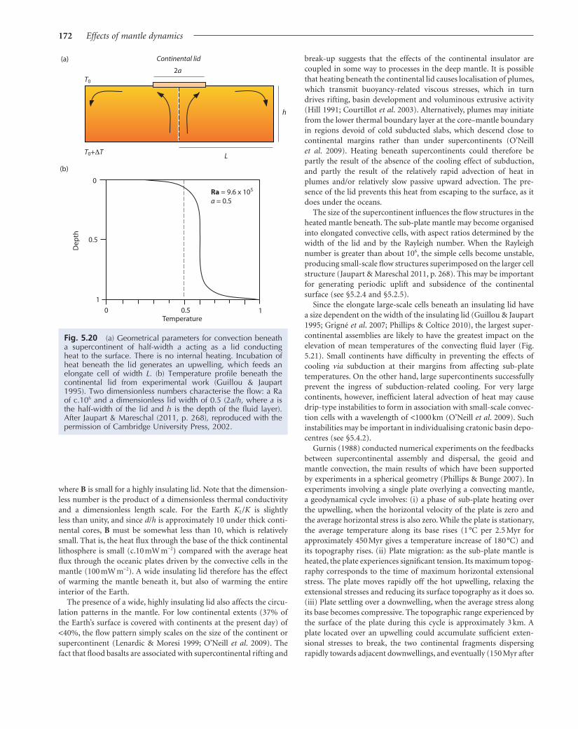
172 Effects of mantle dynamics
break-up suggests that the effects of the continental insulator are
coupled in some way to processes in the deep mantle. It is possible
that heating beneath the continental lid causes localisation of plumes,
which transmit buoyancy-related viscous stresses, which in turn
drives rifting, basin development and voluminous extrusive activity
(Hill 1991; Courtillot et al. 2003). Alternatively, plumes may initiate
from the lower thermal boundary layer at the core–mantle boundary
in regions devoid of cold subducted slabs, which descend close to
continental margins rather than under supercontinents (O’Neill
et al. 2009). Heating beneath supercontinents could therefore be
partly the result of the absence of the cooling effect of subduction,
and partly the result of the relatively rapid advection of heat in
plumes and/or relatively slow passive upward advection. The pre-
sence of the lid prevents this heat from escaping to the surface, as it
does under the oceans.
The size of the supercontinent influences the flow structures in the
heated mantle beneath. The sub-plate mantle may become organised
into elongated convective cells, with aspect ratios determined by the
width of the lid and by the Rayleigh number. When the Rayleigh
number is greater than about 106, the simple cells become unstable,
producing small-scale flow structures superimposed on the larger cell
structure (Jaupart & Mareschal 2011, p. 268). This may be important
for generating periodic uplift and subsidence of the continental
surface (see §5.2.4 and §5.2.5).
Since the elongate large-scale cells beneath an insulating lid have
a size dependent on the width of the insulating lid (Guillou & Jaupart
1995; Grigné et al. 2007; Phillips & Coltice 2010), the largest super-
continental assemblies are likely to have the greatest impact on the
elevation of mean temperatures of the convecting fluid layer (Fig.
5.21). Small continents have difficulty in preventing the effects of
cooling via subduction at their margins from affecting sub-plate
temperatures. On the other hand, large supercontinents successfully
prevent the ingress of subduction-related cooling. For very large
continents, however, inefficient lateral advection of heat may cause
drip-type instabilities to form in association with small-scale convec-
tion cells with a wavelength of <1000 km (O’Neill et al. 2009). Such
instabilities may be important in individualising cratonic basin depo-
centres (see §5.4.2).
Gurnis (1988) conducted numerical experiments on the feedbacks
between supercontinental assembly and dispersal, the geoid and
mantle convection, the main results of which have been supported
by experiments in a spherical geometry (Phillips & Bunge 2007). In
experiments involving a single plate overlying a convecting mantle,
a geodynamical cycle involves: (i) a phase of sub-plate heating over
the upwelling, when the horizontal velocity of the plate is zero and
the average horizontal stress is also zero. While the plate is stationary,
the average temperature along its base rises (1 °C per 2.5 Myr for
approximately 450 Myr gives a temperature increase of 180 °C) and
its topography rises. (ii) Plate migration: as the sub-plate mantle is
heated, the plate experiences significant tension. Its maximum topog-
raphy corresponds to the time of maximum horizontal extensional
stress. The plate moves rapidly off the hot upwelling, relaxing the
extensional stresses and reducing its surface topography as it does so.
(iii) Plate settling over a downwelling, when the average stress along
its base becomes compressive. The topographic range experienced by
the surface of the plate during this cycle is approximately 3 km. A
plate located over an upwelling could accumulate sufficient exten-
sional stresses to break, the two continental fragments dispersing
rapidly towards adjacent downwellings, and eventually (150 Myr after
where B is small for a highly insulating lid. Note that the dimension-
less number is the product of a dimensionless thermal conductivity
and a dimensionless length scale. For the Earth KL/K is slightly
less than unity, and since d/h is approximately 10 under thick conti-
nental cores, B must be somewhat less than 10, which is relatively
small. That is, the heat flux through the base of the thick continental
lithosphere is small (c.10 mW m−2) compared with the average heat
flux through the oceanic plates driven by the convective cells in the
mantle (100 mW m−2). A wide insulating lid therefore has the effect
of warming the mantle beneath it, but also of warming the entire
interior of the Earth.
The presence of a wide, highly insulating lid also affects the circu-
lation patterns in the mantle. For low continental extents (37% of
the Earth’s surface is covered with continents at the present day) of
<40%, the flow pattern simply scales on the size of the continent or
supercontinent (Lenardic & Moresi 1999; O’Neill et al. 2009). The
fact that flood basalts are associated with supercontinental rifting and
Fig. 5.20 (a) Geometrical parameters for convection beneath a supercontinent of half-width a acting as a lid conducting heat to the surface. There is no internal heating. Incubation of heat beneath the lid generates an upwelling, which feeds an elongate cell of width L. (b) Temperature profile beneath the continental lid from experimental work (Guillou & Jaupart 1995). Two dimensionless numbers characterise the flow: a Ra of c.106 and a dimensionless lid width of 0.5 (2a/h, where a is the half-width of the lid and h is the depth of the fluid layer). After Jaupart & Mareschal (2011, p. 268), reproduced with the permission of Cambridge University Press, 2002.
h
L
2a
T0
T0+ T
Temperature
De
pth
0
1
0 0.5
0.5
1
Ra = 9.6 x 10⁵
a = 0.5
Continental lid(a)
(b)
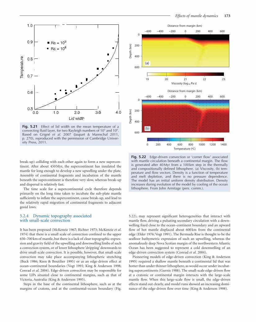
Effects of mantle dynamics 173
5.22), may represent significant heterogeneities that interact with
mantle flow, driving a pulsating secondary circulation with a down-
welling fixed close to the ocean–continent boundary and an upward
flow of hot mantle displaced about 600 km from the continental
edge (Elder 1976; Vogt 1991). The Bermuda Rise is thought to be the
seafloor bathymetric expression of such an upwelling, whereas the
anomalously deep Nova Scotian margin of the northwestern Atlantic
Ocean has been suggested to represent a cold downwelling of an
edge-driven convection system (Conrad et al. 2004).
Pioneering models of edge-driven convection (King & Anderson
1995) required a shallow mantle beneath a continental lid that was
hotter than under thinner lithosphere, as would occur under incubat-
ing supercontinents (Gurnis 1988). The small-scale edge-driven flow
at a cratonic or continental margin interacts with the large-scale
mantle flow. When this large-scale flow is small, the edge-driven
effects stand out clearly, and model runs showed an increasing domi-
nance of the edge-driven flow over time (King & Anderson 1998).
break-up) colliding with each other again to form a new supercon-
tinent. After about 450 Myr, the supercontinent has insulated the
mantle for long enough to develop a new upwelling under the plate.
Assembly of continental fragments and incubation of the mantle
beneath the supercontinent is therefore very slow, whereas break-up
and dispersal is relatively fast.
The time scale for a supercontinental cycle therefore depends
primarily on the long time taken to incubate the sub-plate mantle
sufficiently to inflate the supercontinent, cause break-up, and lead to
the relatively rapid migration of continental fragments to adjacent
geoid lows.
5.2.4 Dynamic topography associated with small-scale convection
It has been proposed (McKenzie 1967; Richter 1973; McKenzie et al.
1974) that there is a small scale of convection confined to the upper
650–700 km of mantle, but there is a lack of clear topographic expres-
sion and gravity field of the upwelling and downwelling limbs of such
a convection system, or of lower lithosphere ‘dripping’ downwards to
drive small-scale convection. It is possible, however, that small-scale
convection may take place accompanying lithospheric stretching
(Buck 1986; Keen & Boutilier 1995) or as an edge-driven effect at
ocean–continental boundaries (Vogt 1991; King & Anderson 1998;
Conrad et al. 2004). Edge-driven convection may be responsible for
some LIPs situated close to continental margins, such as that of
Victoria, Australia (King & Anderson 1995).
Steps in the base of the continental lithosphere, such as at the
margins of cratons, and at the continental–ocean boundary (Fig.
Fig. 5.21 Effect of lid width on the mean temperature of a convecting fluid layer, for two Rayleigh numbers of 105 and 106. Based on Grigné et al. 2007 (Jaupart & Mareschal 2011, p. 270), reproduced with the permission of Cambridge Univer-sity Press, 2011.
Fig. 5.22 Edge-driven convection or ‘corner flow’ associated with mantle circulation beneath a continental margin. The flow is generated after 40 Myr from a 100 km step in the thermally and compositionally defined lithosphere. (a) Viscosity, (b) tem-perature and flow vectors. Density is a function of temperature and melt depletion, and there is no pressure dependence. The model has an initial uniform density distribution. Density increases during evolution of the model by cooling of the ocean lithosphere. From John Armitage (pers. comm.).
0
200
400
600D
ep
th(k
m)
400 600
Distance from margin (km)
0 200 400 600 800 1000 1200 1400
Temperature (ºC)
(b)
0
200
400
600
De
pth
(km
)
−600 −400 −200 0 200
−600 −400 −200 0 200 400 600
Distance from margin (km)
19 20 21 22 23
Viscosity (log10 Pa s)
(a)

174 Effects of mantle dynamics
welling is expected to initiate during the period of continental infla-
tion and extensional break-up. The negative dynamic topography
associated with the downwelling under the continental or cratonic
edge would take the form of low-angle ramp-like tilting towards the
ocean, or sub-circular sags, depending on the three-dimensional
nature of the edge-driven convection (for further discussion see
§5.4.2).
Small-scale convection may also develop under continental litho-
sphere without the effect of a step at the continental edge (Petersen
et al. 2010). The horizontal scale of the temperature variations mod-
elled in the shallow mantle beneath the continental lithosphere is
hundreds of kilometres, representing a considerably smaller length
scale than expected for larger flow structures originating at the core–
mantle boundary (Fig. 5.23). Fluctuations in the dynamic topogra-
A second scenario is that the thick lithosphere is moving relative
to the underlying upper mantle so that there is a shear between the
two. If the mantle moves from the craton to the ocean relative to
the lithosphere, that is, the flow experiences a negative step, the
edge-driven flow maintains itself, but if the relative motion is in the
opposite direction, that is the flow experiences a positive step,
the edge-driven flow is lost in the larger-scale upper-mantle flow.
Consequently, edge-driven circulation and its dynamic topography
is likely to operate when continental assemblies incubate an under-
lying mantle that flows slowly towards the margins. Qualitatively,
elevated bathymetry is expected in the oceanic lithosphere c.103 km
from the continental edge, while the continental lithosphere adja-
cent to the continent–ocean boundary is expected to experience
slow subsidence due to cold downwelling. Such edge-driven down-
Fig. 5.23 Small-scale convection from a numerical convection model (Petersen et al. 2010). (a) Temperature. Black line shows aver-aged model geotherm, and grey line is the isentropic (adiabatic) profile for a potential temperature of 1315 °C. (b) Deviation from the horizontally average temperature. (c) Vertical conductive heat flux; black line is horizontal average. (d) Effective viscosity; black line is horizontal average. Note the development of small-scale instabilities, causing surface variations in heat flow and topography that may be important in the generation of stratigraphic sequences. Reproduced with permission of American Association for the Advancement of Science.
(a)
(b)
(c)
(d)

Effects of mantle dynamics 175
relatively rapid pulses of uplift and subsidence (Fig. 5.25). The dating
of the transient uplift suggests that the uplift-subsidence motion
(150–250 m – greater than can be accounted for by eustatic mecha-
nisms) took place on the time scale of about 106 yr – smaller than the
periods conventionally associated with convection, but similar to the
periodicity of volcanic activity found in some hotspot chains
(O’Connor et al. 2002).
phy of the continental surface of this length scale may explain the
stratigraphic sequences of sedimentary basins.
5.2.5 Pulsing plumes
The periodic emplacement of sand beneath the deep waters of the
North Sea during the Early Tertiary (White & Lovell 1997) (Fig.
5.24b) was interpreted as a result of pulsating activity of the nearby
Iceland plume. Apart from causing variations over time in the
volumes of erupted volcanic rocks (O’Connor et al. 2002), pulsating
plumes might be expected to cause periodic phases of uplift of the
seafloor (or continental surface), leading to the generation of ero-
sional unconformities, tilting of sedimentary strata, and perhaps
even to climate changes caused by the shallowing or occlusion of
oceanographic gateways (Jones et al. 2001; Shaw-Champion et al.
2008; Hartley et al. 2011; Poore et al. 2011). Pulsing plumes may also
cause phases of igneous underplating beneath the crust, resulting in
relative uplift during intrusion followed by subsidence following
crystallisation (McLennan & Lovell 2002).
The transmission of thermal pulses of the early Iceland plume is
thought to have produced diachronous and transient relative uplift
as they spread out from the main plume conduit (Rudge et al. 2008).
The radially spreading mantle material is thought to flow in a channel
of low viscosity beneath the plate, with instabilities giving rise to
Fig. 5.24 (a) Reconstruction of the northern North Atlantic region just after the onset of ocean spreading (magnetic anomaly 23), showing the extent of the Iceland plume (White and McKenzie 1989; reproduced with permission of the American Geophysical Union). Solid shading shows position of extrusive volcanic rocks, and light shading shows extent of Early Cretaceous igneous activity. Uplift over the plume head, shown by circular area, can be recognised in thermochronological data such as apatite fission tracks. (b) Pulsing of the Iceland plume is thought to have caused episodic deposition of sands in the deep sea (White and Lovell 1997; reprinted by permission from Macmillan Publishers Ltd.). Periods of deep-sea fan deposition correspond to times of high levels of intrusive igneous activity.
2000North Atlantic
0 500 1000
km
Lab
rad
or S
ea
Rockall
Greenland
Baffi
n Island
Norw
ay
(a) (b)
2000
Rockall
Greenland
Norw
ay
Fan deposition
Frigg
Balder: 1279km3
Sele: 2768km3
Balmoral–Forties3367km3
Lan
d b
rid
ge
Lan
d b
rid
ge
Andrew14,271km 3
Maureen4789km3
Ekofisk
C28r
C27r
C26r
C25r
C24r
C23r
C22r
Volc
an
ic a
sh b
ed
s
Intr
usi
vem
ag
mati
sm
P7
P6
P5
P4
P3
P1
Dan
ian
Sela
nd
ian
Th
an
eti
an
Yp
resi
an
Eoce
ne
Pale
oce
ne
Ag
e (
Ma)
50
51
52
53
54
55
56
57
58
59
60
61
62
63
64
65
Pla
nkt
ic f
ora
m z
on
es
Mag
neto
stra
tig
rap
hy
Nort
h S
ea f
ield
s
Fig. 5.25 Model for radial, channel-like flow associated with the impingement on the base of the lithosphere of a plume. After Rudge et al. (2008), reprinted with permission from Elsevier.
Region of hotterplume material carriedup plume stem
Upper mantle
Lithosphere Lateral flow inlow-viscositychannel
2h
Region of maximum surface uplift U
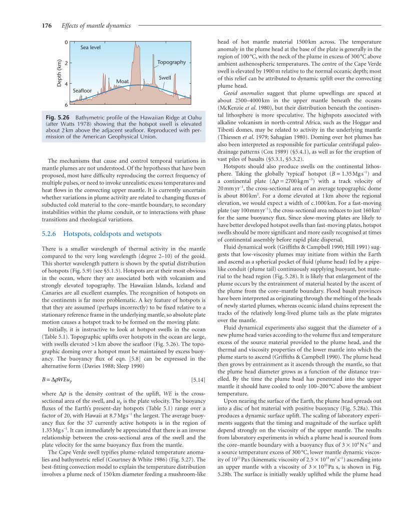
176 Effects of mantle dynamics
head of hot mantle material 1500 km across. The temperature
anomaly in the plume head at the base of the plate is generally in the
region of 100 °C, with the neck of the plume in excess of 300 °C above
ambient asthenospheric temperatures. The centre of the Cape Verde
swell is elevated by 1900 m relative to the normal oceanic depth; most
of this relief can be attributed to dynamic uplift over the convecting
plume head.
Geoid anomalies suggest that plume upwellings are spaced at
about 2500–4000 km in the upper mantle beneath the oceans
(McKenzie et al. 1980), but their distribution beneath the continen-
tal lithosphere is more speculative. The highspots associated with
alkaline volcanism in north-central Africa, such as the Hoggar and
Tibesti domes, may be related to activity in the underlying mantle
(Thiessen et al. 1979; Sahagian 1980). Doming over hot plumes has
also been interpreted as responsible for particular centrifugal paleo-
drainage patterns (Cox 1989) (§5.4.1), as well as for the eruption of
vast piles of basalts (§5.3.1, §5.3.2).
Hotspots should also produce swells on the continental lithos-
phere. Taking the globally ‘typical’ hotspot (B = 1.35 Mg s−1) and
a continental plate (Δρ = 2700 kg m−3) with a track velocity of
20 mm yr−1, the cross-sectional area of an average topographic dome
is about 800 km2. For a dome elevated at 1 km above the regional
elevation, we would expect a width of c.1000 km. For a fast-moving
plate (say 100 mm yr−1), the cross-sectional area reduces to just 160 km2
for the same buoyancy flux. Since slow-moving plates are likely to
have better developed hotspot swells than fast-moving plates, hotspot
swells should be more significant and more easily recognised at times
of continental assembly before rapid plate dispersal.
Fluid dynamical work (Griffiths & Campbell 1990; Hill 1991) sug-
gests that low-viscosity plumes may initiate from within the Earth
and ascend as a spherical pocket of fluid (plume head) fed by a pipe-
like conduit (plume tail) continuously supplying buoyant, hot mate-
rial to the head region (Fig. 5.28). It is likely that enlargement of the
plume occurs by the entrainment of material heated by the ascent of
the plume from the core–mantle boundary. Flood basalt provinces
have been interpreted as originating through the melting of the heads
of newly started plumes, whereas oceanic island chains represent the
tracks of the relatively long-lived plume tails as the plate migrates
over the mantle.
Fluid dynamical experiments also suggest that the diameter of a
new plume head varies according to the volume flux and temperature
excess of the source material provided to the plume head, and the
thermal and viscosity properties of the lower mantle into which the
plume starts to ascend (Griffiths & Campbell 1990). The plume head
then grows by entrainment as it ascends through the mantle, so that
the plume head diameter grows as a function of the distance trav-
elled. By the time the plume head has penetrated into the upper
mantle it should have cooled to only 100–200 °C above the ambient
temperature.
Upon nearing the surface of the Earth, the plume head spreads out
into a disc of hot material with positive buoyancy (Fig. 5.28a). This
produces a dynamic surface uplift. The scaling of laboratory experi-
ments suggests that the timing and magnitude of the surface uplift
depend strongly on the viscosity of the upper mantle. The results
from laboratory experiments in which a plume head is sourced from
the core–mantle boundary with a buoyancy flux of 3 × 10⁴ N s−1 and
a source temperature excess of 300 °C, lower mantle dynamic viscos-
ity of 1022 Pa s (kinematic viscosity of 2.5 × 10¹⁸ m2 s−1) ascending into
an upper mantle with a viscosity of 3 × 10²⁰ Pa s, is shown in Fig.
5.28b. The surface is initially weakly uplifted while the plume head
The mechanisms that cause and control temporal variations in
mantle plumes are not understood. Of the hypotheses that have been
proposed, most have difficulty reproducing the correct frequency of
multiple pulses, or need to invoke unrealistic excess temperatures and
heat flows in the convecting upper mantle. It is currently uncertain
whether variations in plume activity are related to changing fluxes of
subducted cold material to the core–mantle boundary, to secondary
instabilities within the plume conduit, or to interactions with phase
transitions and rheological variations.
5.2.6 Hotspots, coldspots and wetspots
There is a smaller wavelength of thermal activity in the mantle
compared to the very long wavelength (degree 2–10) of the geoid.
This shorter wavelength pattern is shown by the spatial distribution
of hotspots (Fig. 5.9) (see §5.1.5). Hotspots are at their most obvious
in the ocean, where they are associated both with volcanism and
strongly elevated topography. The Hawaiian Islands, Iceland and
Canaries are all excellent examples. The recognition of hotspots on
the continents is far more problematic. A key feature of hotspots is
that they are assumed (perhaps incorrectly) to be fixed relative to a
stationary reference frame in the underlying mantle, so absolute plate
motion causes a hotspot track to be formed on the moving plate.
Initially, it is instructive to look at hotspot swells in the ocean
(Table 5.1). Topographic uplifts over hotspots in the ocean are large,
with swells elevated >1 km above the seafloor (Fig. 5.26). The topo-
graphic doming over a hotspot must be maintained by excess buoy-
ancy. The buoyancy flux of eqn. [5.8] can be expressed in the
alternative form (Davies 1988; Sleep 1990)
B WEup= ∆ρ [5.14]
where Δρ is the density contrast of the uplift, WE is the cross-
sectional area of the swell, and up is the plate velocity. The buoyancy
fluxes of the Earth’s present-day hotspots (Table 5.1) range over a
factor of 20, with Hawaii at 8.7 Mg s−1 the largest. The average buoy-
ancy flux for the 37 currently active hotspots is in the region of
1.35 Mg s−1. It can immediately be appreciated that there is an inverse
relationship between the cross-sectional area of the swell and the
plate velocity for the same buoyancy flux from the mantle.
The Cape Verde swell typifies plume-related temperature anoma-
lies and bathymetric relief (Courtney & White 1986) (Fig. 5.27). The
best-fitting convection model to explain the temperature distribution
involves a plume neck of 150 km diameter feeding a mushroom-like
Fig. 5.26 Bathymetric profile of the Hawaiian Ridge at Oahu (after Watts 1978) showing that the hotspot swell is elevated about 2 km above the adjacent seafloor. Reproduced with per-mission of the American Geophysical Union.
Sea level
Moat
Seafloor
Swell
Topography
0
2
4
6
Dep
th (
km)

Effects of mantle dynamics 177
and perhaps 1000 km in width. The domes of Africa, such as the
Hoggar of the Saharan region, and the Bié and Namibian domes of
southwest Africa (Al-Hajri et al. 2010), are good candidates for uplift
over upwellings. Over geological time, all the continents must have
passed over mantle upwellings, leaving hotspot tracks. Some parts of
continents must have a veritable criss-cross pattern of hotspot tracks
(Morgan 1983). Within a band of approximately 103 km width, the
continental surface should be transiently elevated, leading to erosion
and the development of regional unconformities. Such unconformi-
ties would be recognisable long after the transient dynamic uplift has
ceased. If we ignore flexural uplift due to mountain building (Chapter
4), and dynamic topography related to plate subduction (§5.2.2) and
supercontinental assembly (§5.2.3), involvement in hotspot uplift
may be a major cause for erosional unconformities in cratonic sedi-
mentary sequences.
If there are upwellings beneath continents, we should also expect
there to be downwellings, which would be cold and characterised
by negative dynamic topography. The Congo Basin may be situated
over one such downwelling (Hartley & Allen 1994; Downey &
Gurnis 2009; Crosby et al. 2010, but compare Buiter et al. 2011). It is
situated adjacent to the East African upwelling. The fact that many
is entirely within the lower mantle (−25 Myr). When the plume
head enters the low-viscosity zone of the upper mantle (−3 Myr) the
surface uplift takes place rapidly, reaching a maximum elevation of
600 m after further ascent to just beneath the lithosphere. At this stage
the plume head has a diameter of 1300 km. A number of factors may
increase the maximum elevation of the topographic dome: (i) pen-
etration of the hot plume into the cold lithosphere; and (ii) a volume
increase caused by melting. The release of large amounts of basalts
by melting of the plume can only take place once the plume head has
reached shallow depths. It should be noticed that this is only possible
a number of millions of years after the maximum surface uplift. The
development of smaller-scale gravitational instabilities over the cap
of the plume as cold, dense material is squeezed between the ascend-
ing plume head and the Earth’s surface may facilitate the last-stage
ascent of the plume and produce the high surface uplifts seen today
in locations such as East Africa, and the large outpourings of basalts
in the geological past, such as the Siberian and Deccan (India) Traps
(Fig. 5.8).
Hotspot swells in the oceans are well documented. We might also
expect topographic uplift of the continents over sub-lithospheric
upwellings. Such uplifts are likely to be of the order of 1 km in height
Fig. 5.27 Cape Verde hotspot. (a) Bathymetric map (in m) of the Cape Verde Rise, with isochrons in Ma. Fracture zones are shown in dashed lines. (b) Heat flow, surface uplift and the geoid for a convection cell at 4000 times the critical Rayleigh number for convec-tion. The total uplift is shown as a conductive component (dashed) and a convective component (dotted). (c) Temperature distribution responsible for the results shown in (b). After Courtney & White (1986), reproduced with permission of Oxford University Press.
110
125
140
155
1000
2000
3000
40005000
5000
4000
Bahamas FZ
Kane FZ
Cape Verde
Islands
Blake Spur FZ
West
Afr
ica
30 °W 25 ° 20 ° 15 °W
25 °N
20 °
15 °
10 °N
20
0
–20
Heat
flow
(mW
m–2)
0 400 800200 600
Distance (km)
Geoid
(m
)
30
20
10
0
6
4
2
0
–2
Surf
ace
up
lift
(km
)
Ra =4000x Racrit(a)
(b)
(c)
1300
1100
900700Upwelling
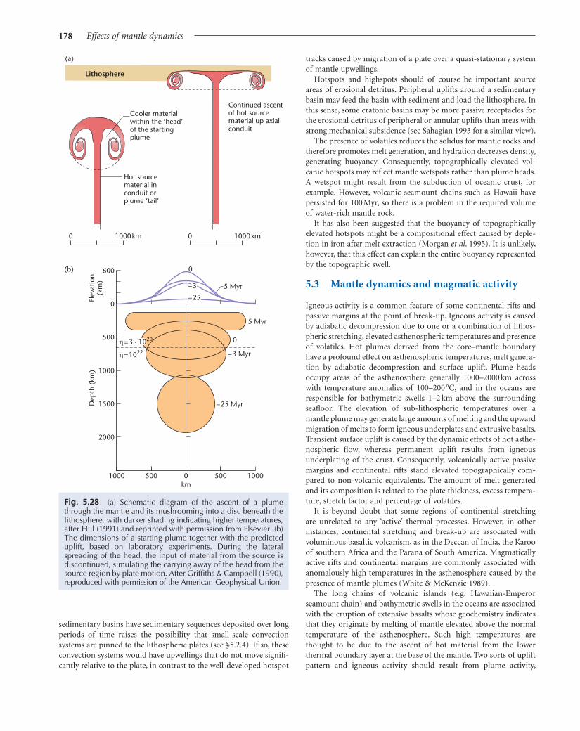
178 Effects of mantle dynamics
tracks caused by migration of a plate over a quasi-stationary system
of mantle upwellings.
Hotspots and highspots should of course be important source
areas of erosional detritus. Peripheral uplifts around a sedimentary
basin may feed the basin with sediment and load the lithosphere. In
this sense, some cratonic basins may be more passive receptacles for
the erosional detritus of peripheral or annular uplifts than areas with
strong mechanical subsidence (see Sahagian 1993 for a similar view).
The presence of volatiles reduces the solidus for mantle rocks and
therefore promotes melt generation, and hydration decreases density,
generating buoyancy. Consequently, topographically elevated vol-
canic hotspots may reflect mantle wetspots rather than plume heads.
A wetspot might result from the subduction of oceanic crust, for
example. However, volcanic seamount chains such as Hawaii have
persisted for 100 Myr, so there is a problem in the required volume
of water-rich mantle rock.
It has also been suggested that the buoyancy of topographically
elevated hotspots might be a compositional effect caused by deple-
tion in iron after melt extraction (Morgan et al. 1995). It is unlikely,
however, that this effect can explain the entire buoyancy represented
by the topographic swell.
5.3 Mantle dynamics and magmatic activity
Igneous activity is a common feature of some continental rifts and
passive margins at the point of break-up. Igneous activity is caused
by adiabatic decompression due to one or a combination of lithos-
pheric stretching, elevated asthenospheric temperatures and presence
of volatiles. Hot plumes derived from the core–mantle boundary
have a profound effect on asthenospheric temperatures, melt genera-
tion by adiabatic decompression and surface uplift. Plume heads
occupy areas of the asthenosphere generally 1000–2000 km across
with temperature anomalies of 100–200 °C, and in the oceans are
responsible for bathymetric swells 1–2 km above the surrounding
seafloor. The elevation of sub-lithospheric temperatures over a
mantle plume may generate large amounts of melting and the upward
migration of melts to form igneous underplates and extrusive basalts.
Transient surface uplift is caused by the dynamic effects of hot asthe-
nospheric flow, whereas permanent uplift results from igneous
underplating of the crust. Consequently, volcanically active passive
margins and continental rifts stand elevated topographically com-
pared to non-volcanic equivalents. The amount of melt generated
and its composition is related to the plate thickness, excess tempera-
ture, stretch factor and percentage of volatiles.
It is beyond doubt that some regions of continental stretching
are unrelated to any ‘active’ thermal processes. However, in other
instances, continental stretching and break-up are associated with
voluminous basaltic volcanism, as in the Deccan of India, the Karoo
of southern Africa and the Parana of South America. Magmatically
active rifts and continental margins are commonly associated with
anomalously high temperatures in the asthenosphere caused by the
presence of mantle plumes (White & McKenzie 1989).
The long chains of volcanic islands (e.g. Hawaiian-Emperor
seamount chain) and bathymetric swells in the oceans are associated
with the eruption of extensive basalts whose geochemistry indicates
that they originate by melting of mantle elevated above the normal
temperature of the asthenosphere. Such high temperatures are
thought to be due to the ascent of hot material from the lower
thermal boundary layer at the base of the mantle. Two sorts of uplift
pattern and igneous activity should result from plume activity,
Fig. 5.28 (a) Schematic diagram of the ascent of a plume through the mantle and its mushrooming into a disc beneath the lithosphere, with darker shading indicating higher temperatures, after Hill (1991) and reprinted with permission from Elsevier. (b) The dimensions of a starting plume together with the predicted uplift, based on laboratory experiments. During the lateral spreading of the head, the input of material from the source is discontinued, simulating the carrying away of the head from the source region by plate motion. After Griffiths & Campbell (1990), reproduced with permission of the American Geophysical Union.
0 1000km 0 1000km
Cooler materialwithin the ‘head’of the startingplume
Hot sourcematerial inconduit orplume ‘tail’
Continued ascentof hot sourcematerial up axialconduit
(a)
Lithosphere
00010001 500 0 500
600
0
500
1000
1500
2000
Dep
th (
km)
Ele
vati
on
(km
)
0
–25
–3 5 Myr
5 Myr
–25 Myr
–3 Myr
0
(b)
η=1022
η=3·1020
km
sedimentary basins have sedimentary sequences deposited over long
periods of time raises the possibility that small-scale convection
systems are pinned to the lithospheric plates (see §5.2.4). If so, these
convection systems would have upwellings that do not move signifi-
cantly relative to the plate, in contrast to the well-developed hotspot

Effects of mantle dynamics 179
depending on whether the lithosphere overlies a plume head or
plume tail. Plume head regions should be areally extensive and
equant (1500 km to 2500 km across), giving rise to LIPs, whereas
plume tail provinces should be narrow (<300 km wide) and linear,
that is, they should be hotspot tracks.
5.3.1 Melt generation during continental extension
Igneous activity in sedimentary basins is diagnostic of basin-forming
mechanisms. In the reference uniform stretching model of McKenzie
(1978a), no melts are generated because the geotherm does not inter-
sect the solidus for crustal and mantle materials. However, it is well
known that rift provinces are associated with minor (e.g. Western
Rift, Africa, North Sea) to major (Eastern Rift, Africa, Rio Grande)
volcanism. Most importantly, continental break-up at high values of
stretching is commonly associated with vast outpourings of flood
basalts, indicating major melting of the asthenosphere by adiabatic
decompression. Melts liberated by decompression are assumed to
separate from their residue and to travel upwards to either be erupted
at the surface, or to be emplaced as igneous bodies in the crust.
McKenzie and Bickle (1988) showed how the amount of melt gener-
ated depends on the potential temperature of the asthenosphere –
defined as the temperature the asthenosphere would have if brought
to the surface adiabatically without melting – and the amount of
stretching (Fig. 5.29). For example, if a 100 km-thick lithosphere
is stretched by a factor of 2, we would expect a melt thickness of
about 2 km for a potential temperature of 1400 °C. At higher values
of stretching (β = 5), we would expect a melt thickness of 10 km for
the same potential temperature. The normal potential temperature
of the asthenosphere is 1280 ± 30 °C, so the examples above refer to
an excess temperature of the order of 100 °C attributable to plume
activity.
The conditions at the site of partial melting are reflected in the
composition of the erupted basalts. Stretching at infinitely high
values at a normal asthenospheric potential temperature of 1280 °C
produces melt with the composition of a mid-ocean ridge basalt
(MORB). However, increasing the potential temperature to 1480 °C
causes an increase in MgO and a decrease in Na2O. Consequently, we
would anticipate the generation of first alkali basalts and then tho-
leiitic basalts as stretching increases over an asthenosphere with a
potential temperature of 1480 °C.
The presence of a hot asthenosphere affects the subsidence expe-
rienced at the Earth’s surface caused by lithospheric stretching. This
is mainly caused by two effects: the addition of igneous bodies
beneath the crust (see below), and the dynamic uplift from the
mantle plume.
The density of igneous rock generated by adiabatic decompression
of the mantle depends on the potential temperature at the site of
partial melting, and ranges between 2990 and 3070 kg m−3 (at a depth
of 10 km) for potential temperatures of 1280 °C and 1480 °C respec-
tively. This range of density is mid-way between the density of the
continental crust and the density of the mantle, so there is a strong
likelihood that melts will be trapped and underplated beneath the
crust. Since these igneous additions replace lithospheric mantle
(density 3300 kg m−3), the net effect is uplift relative to the depth
expected from uniform stretching of the lithosphere without mag-
matic activity (Appendix 27).
Assuming Airy isostasy, the amount of underplating X required to
generate an amount of surface uplift U can be found by balancing
Fig. 5.29 Melt generation by adiabatic decompression during pure shear extension, based on McKenzie & Bickle (1988), White & McKenzie (1989) and Latin & White (1990). (a) Uniform stretching of the lithosphere by a stretch factor of 2. (b) Adiabatic upwelling due to stretching at different values of β from 1.5 to 50. Potential temperature of the asthenosphere 1280 °C, mechanical boundary layer thickness of 100 km, kinematic viscosity 4 × 10¹⁵ m2 s−1. Curves between the liquidus and the solidus show the melt fraction by weight. Only small amounts of melt can be produced at high values of stretching. (c) As for (b), but with a potential temperature of 1480 °C, showing that large amounts of melt can be liberated at relatively low values of the stretch factor.
yc
yL
1100 1300 1500 1700 1900 2100
50
100
150
0
1
2
3
4
5
Temperature ( C)
Pre
ssure
(G
Pa)
Dep
th (
km)
Liquid
us
0.7
00.4
38
1100 1300 1500 1700 1900 2100
Temperature ( C)
0
1
2
3
4
5
Pre
ssure
(G
Pa)
0.2450
50
100
150D
ep
th (
km)
0
0.1
5So
lidus
50
543
2
1.5
Liquid
us0.7
00.4
38
Solid
us
0.1
5
0.245
50
543
2
1.5
(a)
(b)
(c)
b=2
Pure shear
Asthenosphere
Moho

180 Effects of mantle dynamics
5.3.3 The northern North Atlantic and the Iceland plume
The northern Atlantic contains extensive basalts covering c.500 ×
103 km2 on both sides of the ocean in Greenland and in northwest
Britain, Ireland and the Faroes (Fig. 5.24). The basalts range from
52–63 Ma in age, with a main eruption phase at 59 Ma (Mussett et al.
1988). The thermal anomaly responsible for these igneous provinces
is now located beneath Iceland. The Iceland region continues to be
dynamically supported by the underlying plume over an area of
anomalously shallow seafloor with a radius of 1000 km.
In the subsurface seismic record, extrusive basalt sheets can be
recognised as seaward-dipping reflectors along both the east Green-
land and Rockall–Faroes–Norwegian margin. Volumetrically smaller
basaltic volcanism can be seen in onshore exposures such as the
Tertiary Igneous province of northwest Scotland and northeast
Ireland. Thick (<8 km) prisms of accreted igneous rocks with seismic
velocities >7.2 km s−1 have been imaged across the Hatton Bank and
Voring Plateau beneath thinned continental crust, most likely repre-
senting underplated igneous rocks. White and McKenzie (1989)
estimate the combined underplate and extrusive basalt volume as
<107 km3.
The Icelandic plume has been identified as the ‘smoking gun’ for
the widespread surface uplift of the North Atlantic area in the Early
Tertiary (Paleocene). The regional surface uplift caused by under-
plating and dynamic support is thought to have promoted high rates
of denudation and transport of particulate load into the deep-sea
environments of the North Sea and NW Atlantic margin basins.
High rates of denudation in large areas of northwestern Europe
during the Early Tertiary can be inferred from apatite fission track
analysis (papers in Doré et al. 2002). In the neighbouring sedimen-
tary basins, such as the Faroes–Shetland Basin and the Rockall–
Porcupine troughs, sandstones were episodically delivered from this
exhuming continental landmass. White and Lovell (1997) suggested
that the main pulses of submarine fan deposition correspond to the
main pulses of magmatic activity during the time period 62 to
54 Ma.
5.3.4 The Afar region, Ethiopia
The Afar region of northeast Africa is currently undergoing exten-
sion, accompanied by voluminous intrusive and extrusive mag-
matism. It illustrates the magmatism associated with continental
break-up and the transition to a new ocean basin, during continental
rifting (Ebinger & Casey 2001). The uppermost mantle beneath the
Horn of Africa (to a depth of 400 km) is seismically (P- and S-waves)
slow (7.4–7.5 km s−1) (Fig. 5.30), suggesting that the mantle is hot and
most likely subject to partial melting. It has been suggested that the
mantle beneath Ethiopia is the hottest on Earth (Bastow et al. 2008).
One view is that the Ethiopian region is the location of a plume stem
originating from a northward continuation of the African super-
plume (Furman et al. 2006) – a deep, long-lived, thermal structure
with a footprint on the core–mantle boundary of 2000 × 4000 km
and a height of 2000 km. An alternative view is that it is part of a
single large plume centred on Turkana (Ebinger & Sleep 1998), and
a further possibility is of two plumes rising beneath southern Ethio-
pia and Afar (Rogers et al. 2000).
A characteristic feature of continental rift provinces overlying hot
mantle is that a large (∼80%) part of the extension is achieved by the
two lithospheric columns. In the undisturbed column, crust of thick-
ness yc and density ρc occurs within a lithosphere of thickness yL and
subcrustal density ρm. In the underplated lithospheric column, crust
of the same thickness is underlain by a layer of basaltic underplate
with thickness X and density ρx. The total thickness of this lithos-
pheric column is yL plus the surface uplift U.
Balancing the pressures at a depth of compensation at the base of
the lithosphere yields
U Xx
m
= −
1ρρ
[5.15]
The density of the mantle lithosphere can be taken as 3300 kg m−3
and the density of the basaltic underplate as 3000 kg m−3. The rock
uplift for an underplate thickness of 5 km is therefore 455 m, or
approximately one tenth of the underplate thickness. This is also the
surface uplift without any erosion. We can incorporate erosion in the
simplest way as follows (Brodie & White 1994). Consider a piece of
lithosphere underplated with basalt of thickness X that is eroded so
that the surface elevation change is zero (Fig. A27.1). The crust there-
fore has a thickness of yc minus the denudation D. We can once again
perform an isostatic balance, giving
D Xm x
m c
=
−−
ρ ρρ ρ
[5.16]
where D is the total denudation of crust caused by the emplacement
of a basaltic underplate of thickness X. The total denudation for an
underplate thickness of 5 km if there is no change in the surface
elevation is 2.5 km, if crustal rocks of density 2700 kg m−3 are eroded.
We therefore have the maximum erosion case and the no-erosion
case. Reality is probably in between. Clearly, magmatic underplating
can have significant effects on surface uplift and on the delivery
of erosional products to neighbouring sedimentary basins (White
& Lovell 1997). The uplift caused by magmatic underplating is
permanent.
The circulation in the mantle plume maintains anomalously high
temperatures that cause a dynamic uplift, as described above. The
combined effect of underplating and dynamic support is to elevate
the continental plate to sea level or above during the rifting process
for excess asthenospheric temperatures of 100–150 °C. This is entirely
supported by the observation that the basalts erupted at rifted con-
tinental margins are commonly subaerial rather than submarine, and
flow for large distances downslope to produce extensive flood basalt
provinces.
5.3.2 Large igneous provinces
It is known that hotspot tracks emerge from LIPs, or flood basalt
provinces (Morgan 1981). The tracks are marked by volcanoes with
an age progression along the chain, highly suggestive of the relative
movement of the oceanic plate across a plume tail. The end of the
track is a currently active volcano. Correspondingly, large equant
igneous provinces are interpreted as the result of impingement of a
plume head on the base of the lithosphere. The largest submarine
flood basalt province is the Ontong Java Plateau east of Papua New
Guinea, whereas the Siberian traps of northwestern Russia, the Karoo
of southern Africa, and the Parana of South America are celebrated
continental flood basalt provinces from the geological record
(Duncan & Richards 1991).

Effects of mantle dynamics 181
north at ∼10 Ma. The coincidence of the onset of topographic uplift
and the onset of extrusive volcanism at 30 Ma suggest that they both
relate to the arrival of a hot mantle flow structure beneath the area,
though whether it was a plume head (Griffiths & Campbell 1990; Hill
1991) followed by a narrow conduit or tail, is unknown. Early dyking
controlled the orientation of later border faults, which accommo-
dated most slip some millions of years later.
5.4 Mantle dynamics and basin development
Mantle dynamics influence basin development in a number of pos-
sible ways. Principally, mantle processes control dynamic topography
(§5.2), which has an important impact on the location and elevation
of source regions for sediment and on the location and rate of subsid-
ence of sedimentary basins. However, extracting the component of
dynamic topography from the total topographic signal of the surface
of the Earth and from its sedimentary archive is challenging. The
most promising situations are areas where other basin-forming
mechanisms are absent or subdued, such as in continental interiors.
Cratonic basins (§5.4.2) therefore offer the possibility of inverting
mantle processes from the stratigraphic record.
Topography supported by convective flow in the mantle occurs at
different wavelengths and amplitudes. The dynamic topography due
to the African superplume (Nyblade & Robinson 1994) is approxi-
mately 500 m over a large part of the African continent, whereas the
dynamic topography related to the convective cells responsible for
hotspots is likely to be 0.5–1 km over a much shorter wavelength of
500–1000 km. In addition, a number of domal uplifts occur close
to the ocean–continent transition in western Africa, such as the
Namibian dome (Al-Hajri et al. 2010).
5.4.1 Topography, denudation and river drainage
It is a challenging problem to estimate the dynamic topography of
the continental surface in the geological past. One approach is to
map the stratigraphic gaps of unconformities attributable to dynamic
support, and to convert denudation estimates to amounts of topo-
graphic uplift. Phases of uplift also correspond to pulses of increased
sediment delivery to offshore sedimentary depocentres (Walford
et al. 2005). This procedure has been carried out, for example, in the
late Cenozoic domal uplifts in southwestern Africa (Al-Hajri et al.
2010) (Fig. 5.31). Whereas a phase of Oligocene uplift is attributed
to the initiation of the African superplume, a Pliocene unconformity
suggests the rapid emergence of a number of smaller domes around
the western perimeter of the superplume.
Surface uplift of the continental surface affects the course of river
systems draining the elevated region. Centrifugal drainage patterns
may develop over domal uplifts (Cox 1989). River long profiles
potentially contain information about the uplift history experienced
by the drainage area (Roberts & White 2009; Pritchard et al. 2009),
since erosional landscapes respond to relative uplift by the upstream
passage of a wave of erosion recognised by a knickzone (Fig. 5.32)
(Appendix 47). When applied to African examples (Fig. 5.31), where
topography is expected to reflect convective circulation (Burke &
Gunnell 2008), a coherent picture of surface uplift, denudation and
sediment supply to the ocean is obtained. In the magmatic domes
of Hoggar and Tibesti of Saharan Africa, and the amagmatic domes
of Bié, Namibia and South Africa, uplift started 30–40 millions of
years ago. A further application to the rivers of the Colorado Plateau
intrusion of dykes, as occurs below the Baikal rift (Thybo & Nielsen
2009). This means that stretch factors are relatively low, which affects
the timing and volume of decompression melts generated by thin-
ning during advanced stages of plate break-up. Magma intrusion also
reduces plate strength, thereby causing later localisation of stretching.
The Main Ethiopian Rift is consequently displaced towards its eastern
edge from the locus of the underlying low-velocity zone.
The final stretching leading to a new ocean basin caused volumi-
nous (2 km thick) basaltic volcanism due to decompression melting
of the asthenosphere at 29–31 Ma. This is just prior to, or at the same
time as the onset of rifting in the Red Sea and Gulf of Aden. These
flood basalts of the NW Plateau directly overlie the low-velocity zone
in the upper mantle. Active volcanism continues to the present day
in the Afar Depression and parts of the Main Ethiopian Rift. Low-
temperature thermochronometry suggests that Ethiopia experienced
surface uplift at 30–20 Ma. Extension in the Main Ethiopian Rift
started at ∼20 Ma in the south of the region, but migrated to the
Fig. 5.30 Vertical cross-sections of the P-wave velocity model, with contours in P-wave velocity anomaly (%), for (a) the con-tinental rifting part of the Ethiopian region, and (b) the region of transition to ocean crust towards Afar. The low-velocity zone extends from 75–400 km depth and is thought to be the north-ward continuation of the African superplume. The very slow velocities are thought to be due to partial melting in the upper mantle. The Main Ethiopian Rift (MER) is situated towards the eastern flank of the low-velocity structure, not above its centre, suggesting that pre-existing tectonic structures are important in localising melt migration at the base of the lithosphere. From Bastow et al. (2008), reproduced with permission of John Wiley & Sons, Inc.
km
km
(a)
(b)

182 Effects of mantle dynamics
Fig
. 5.3
1
Long-
wav
elen
gth f
ree-
air
grav
ity
map
of
Afr
ica,
fro
m R
ob
erts
& W
hit
e (2
01
0),
sh
ow
ing
po
siti
ve (
red
) an
d n
egat
ive
(blu
e) a
no
mal
ies,
co
nto
ure
d a
t 5
mG
al.
Th
e lo
ng-
wav
elen
gth g
ravi
ty a
nom
alie
s m
ay r
epre
sent
con
vect
ive
circ
ula
tio
n b
enea
th t
he
lith
osp
her
e. B
oxe
d p
osi
tive
an
om
alie
s ar
e to
po
grap
hic
do
mes
wh
ere
rive
rs h
ave
bee
n
anal
ysed
in o
rder
to e
stim
ate
the
tim
ing
of
upli
ft e
ven
ts f
rom
kn
ickp
oin
ts.
H,
Ho
ggar
; T
, T
ibes
ti;
B,
Bié
do
me;
N,
Nam
ibia
n d
om
e; S
, So
uth
Afr
ica
do
me.
Riv
ers
wh
ose
lo
ng
pro
file
s w
ere
use
d a
re s
how
n i
n t
he
inse
t m
aps.
Rep
rod
uce
d w
ith
per
mis
sio
n o
f th
e A
mer
ican
Geo
ph
ysic
al U
nio
n.
So
uth
Afr
ica
do
me
(S
)
Na
mib
ian
do
me
(N
)
Bié
do
me
(B
)
01
00
20
0
Kilo
me
ters
05
01
00
Kilo
me
ters
04
08
0
Kilo
me
ters
07
01
40
Kilo
me
ters
07
51
50
Kilo
me
ters
3
2
1
3
3
3
2
2
2
1
1
1
3
2
1
40
º
20
º
–2
0º
–4
0º 3
40
º0
º2
0º
40
º
0º
Ho
gg
ar
(H)
Tib
est
i (T
)
Lon
g-w
ave
len
gth
fre
e-a
ir g
rav
ity
an
om
aly

Effects of mantle dynamics 183
Fig. 5.32 Look-up chart for estimating the timing of uplift events from the position of knickpoints along the river profile. Erosion parameters are advective coefficient v = 50 m1−m Myr−1, exponent for distance m = 0.5, and erosional diffusivity κ = 105 m2 Myr−1 . Numbered curves are isochrons in Myr, which give the timing of the uplift event for a given knickpoint distance from the river mouth. Shown on look-up chart are three rivers from the Bié dome, southwest Africa (open circles), and three rivers from the South Africa dome (open triangles), each with 2 or 3 knickpoints. From Roberts & White (2010, fig. 15), repro-duced with permission of the American Geophysical Union. See also Appendix 47.
0
0
100
105
100
200
20
200
300
30
Riv
er
len
gth
, km
300
400
40
400
500
500
600
600
700
700
800
800
900
900
1000
1000
1100
1100
12001200
Knickpoint distance from mouth, km
region, which experienced uplift over the Yellowstone hotspot, also
yielded valuable information on the timing and amount of dynamic
topography (Roberts et al. 2012).
It is argued that rapid changes in Miocene shoreline positions and
a change in flow direction of the paleo-Amazon River took place as
a result of surface elevation changes driven by the subduction of
oceanic slabs beneath the South American continent (Shephard et al.
2010) (Fig. 5.33). The impact of mantle dynamics on drainage
network is also seen in the case of the Yellowstone hotspot (Beranek
et al. 2006; Wegmann et al. 2007).
The rate of motion of an overlying plate relative to a mantle flow
structure should determine the amplitude, wavelength and longevity
of topographic uplift. Let us take two contrasting situations. In the
first case of a rapidly moving plate relative to the mantle, such as
the northward movement of the Australian plate in the Pliocene to
Recent (Heine et al. 2010), the uplift is short-lived and relative sea-
level changes, recognised by shoreline migration, regionally variable.
In the second case of a slowly moving plate relative to the mantle,
shoreline migration may be uniform over very large distances, giving
the impression of a eustatic control.
5.4.2 Cratonic basins
Among the many hypotheses for the formation of cratonic basins
(Allen & Armitage 2012 for summary), a common theme is the
thermal contraction of the lithosphere following heating (Sleep &
Snell 1976; Xie & Heller 2009). Cratonic basins are described and
discussed in relation to lithospheric stretching in §3.2.1. Models of
stretching of a continental plate assume that the basal boundary is
isothermal (McKenzie 1978a) or experiences a constant heat flow
(Kaminski & Jaupart 2000). Instead, the base of the lithosphere can
be treated as the boundary between a ‘stagnant’ or insulating conti-
nental lid and a convecting underlying mantle (Sleep 2009). In this
case the uplift and subsidence of the Earth’s surface constitutes
dynamic topography.
Dynamic topography may therefore be manifested on the conti-
nents at the present day, apart from the distribution of hotspots and
highspots (§5.2.6), in the regions of sag-like subsidence of cratonic
basins (Fig. 5.34). The Eyre Basin of Australia (Alley 1998; Veevers
et al. 1982), the Congo Basin of Africa (Downey & Gurnis 2009) and
the Hudson Bay of Canada (Hanne et al. 2004) are potentially exam-
ples. Some workers have suggested that basins of this type, such as
the Congo Basin, are located over downwellings of convective cells
in the mantle (Hartley & Allen 1994; Heine et al. 2008; Downey &
Gurnis 2009). This would explain the lack or paucity of evidence for
stretching of the continental crust under some cratonic basins (Allen
& Armitage 2012). If cratonic basins are located over downwellings,
these convective cells must be attached to the overlying plate, since
the locus of subsidence stays fixed relative to the continental crust
for protracted periods of time, despite relative motion of plates with
respect to the stationary reference frame of the sub-plate mantle.
Other workers attribute sag-type subsidence to the ponding of plume
material in a closed region beneath the continental plate caused by
thinning (Sleep 2009).
The subsidence histories revealed by stratigraphic thicknesses pen-
etrated in boreholes in cratonic basins can be matched by predictions
from a range of models, including slow strain rate uniform stretching
of an initially thick lithosphere (Armitage & Allen 2010) as well as
those invoking dynamic effects transmitted from an underlying con-
vecting mantle.
5.4.3 The history of sea-level change and the flooding of continental interiors
Since the oceanic lithosphere is the cooled thermal boundary layer
of the underlying mantle convection system, its root-age trend for
ocean bathymetry should play an important role in controlling long-
term global sea level through its effect on ocean basin volume. This
effect may operate in a number of ways: (i) changes over time in the
temperature of the upper mantle beneath the oceanic plates could
conceivably result in long-term global sea-level changes. As an illus-
tration of this potential, it is known that the depth of the mid-ocean
ridge crests, where unaffected by plumes, varies broadly over a depth
range of 1 km. A modest temperature change in the upper mantle of
just 40–50 °C would generate this order of variation in seafloor
topography. If the thermal structure of the mantle changed signifi-
cantly over geological time, such changes might be manifested in
variations in the extent to which continents are flooded. (ii) Growth
in the size of a newly formed ocean basin would cause a temporal
increase in the average age of the ocean floor, and therefore an
increase in the volume of the ocean basin, with no change in the
production rate of new seafloor (Xu et al. 2006). This process has
been used to explain the Cenozoic sea-level fall as a result of the
progressive aging of the world’s ocean basins.
If the root-age depth of the ocean floor of the form d = a + bt1/2
(where d is seafloor depth, t is age, and a and b are constants), or
thermal topography, is subtracted from the observed seafloor bathym-
etry (Davies & Pribac 1993), the mid-ocean ridges are removed, and
a broad swell is observed in the central and western Pacific, with a
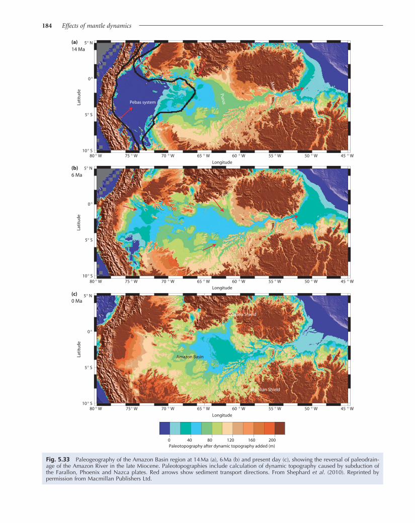
184 Effects of mantle dynamics
Fig. 5.33 Paleogeography of the Amazon Basin region at 14 Ma (a), 6 Ma (b) and present day (c), showing the reversal of paleodrain-age of the Amazon River in the late Miocene. Paleotopographies include calculation of dynamic topography caused by subduction of the Farallon, Phoenix and Nazca plates. Red arrows show sediment transport directions. From Shephard et al. (2010). Reprinted by permission from Macmillan Publishers Ltd.
0 40 80 120 160 200
80 ° W10° S
5° S
0°
50 Ma
6 Ma
14 Ma
° N
10° S
5° S
0°
5° N
10° S
5° S
0°
5° N
75° W 70 ° W 65 ° W 60 ° W 55 ° W 50 ° W 45 ° W
80 ° W 75 ° W 70 ° W 65 ° W 60 ° W 55 ° W 50 ° W 45 ° W
80 ° W 75 ° W 70 ° W 65 ° W 60 ° W 55 ° W 50 ° W 45 ° W
Guyana Shield
Amazon Basin
Brazilian Shield
An
de
ss
Paleotopography after dynamic topography added (m)
Pebas system
Pu
rus
Mo
nte
A.
(a)
(b)
(c)
La
titu
de
La
titu
de
La
titu
de
Longitude
Longitude
Longitude

Effects of mantle dynamics 185
the uplift of the superswell most likely reduced the volume of the
ocean basins and displaced water over the continental shelves, causing
the sea-level highs characteristic of this period of Earth history (Bond
1978). Assuming a 5000 km-wide superswell of roughly circular
planform shape, with an average bathymetric elevation above the
regional bathymetry of 500 m, gives a volume of displaced water of
10 × 106 km3. Since the area of ocean surface is 360 × 106 km2, and
neglecting isostatic compensation, the global water depth increase
is approximately 25–30 m, from the effect of one superswell alone.
If the effects of thermal expansion of the Cretaceous ocean is
also included, the continents are expected to have been inundated
extensively during the Cretaceous, as is confirmed from the trans-
gressive nature of marine stratigraphy of this age (Bond 1976, 1978)
(Fig. 8.23).
broad low observed between Australia and Antarctica (residual
topography, Fig. 5.14). The south Pacific feature, several thousand
kilometres in extent and hundreds of metres in elevation, is known
as a superswell (McNutt & Fischer 1987; McNutt 1998; Adam &
Bonneville 2005). Superswells correspond to regions of slow seismic
velocities from tomographic studies, and with an anomalously high
geoid. These observations suggest that superswells overlie relatively
warm mantle. They are regions that have escaped the cooling effects
of subduction for long (100–200 Myr) periods of time.
Superswells undoubtedly formed in the past. In the south Pacific
region, seafloor updoming in the Cretaceous was accompanied by
the eruption of flood basalts (Ontong Java Plateau) due to the spawn-
ing of new plumes in the heated region below the superswell (Davies
& Pribac 1993) (Fig. 5.35). The importance of this observation is that
Fig. 5.34 Mantle circulation may be involved in the evolution of some cratonic basins, such as the Congo Basin (after Downey & Gurnis 2009). Convective circulation in the mantle may be responsible for the late Cenozoic to present-day subsidence of the basin and the uplift of the surrounding annulus (Hartley & Allen 1994; Crosby et al. 2010; Downey & Gurnis 2009). (a) Sediment isopachs showing roughly circular basin outline with subsidiary depocentres. Yellow circles are borehole locations. (b) to (f) show sequential evolution from Neoproterozoic to present-day. Reproduced with permission of John Wiley & Sons, Inc.
Thick lithosphere, 600 Ma(b)
(d)
(e)
(f )
(c)
(a)
10˚
5˚
0˚
–5˚
–10˚
30˚25˚20˚15˚10˚
86420 10
crust
mantle
lithosphere
Neoproterozoic extension
Minor Cambro-Ordovician shortening (erosion)
Regional Cenozoic uplift (Southern African superswell)
Sediment thickness (km)
Present-day dynamic topography
sea level

186 Effects of mantle dynamics
Fig. 5.36 Effect of dynamic topography on estimates of eustatic sea level, after Spasojevic et al. (2008). (a) Predicted dynamic topog-raphy in North America and the western Atlantic Ocean based on a mantle convection model, with the red circle showing the location of the New Jersey coastal plain. (b) Difference between predicted dynamic topography at 50 Ma (early Eocene) and the present day. The results in (a) and (b) are consistent with the position of paleoshorelines on the coastal plain of eastern USA, and explain some of the discrepancies in Fig. 8.23. Reproduced with permission of the American Geophysical Union.
(a) (b)
Fig. 5.35 Possible evolution of the Pacific mantle and superswell during the Cretaceous, after Davies & Pribac (1993). In (a) a region of mantle between two subduction zones warms up and causes a thermal doming of the Earth’s surface, causing extension. The warming promotes the formation of new plumes that cause igneous accretions to the overlying plate (b). Gen-erations of plumes and their igneous products are formed and transported away through plate motion (c). Note that Davies & Pribac (1993) invoke a large region of mantle heating that spawns plume activity rather than a ‘super-plume’. Reproduced with permission of the American Geophysical Union.
Extension
Subduction CoolingWarming - upflow
Botto
m thermal boundary layer
Extension
Plumes
Extension
Plumes
Extensive intraplate volcanism
(a)
(b)
(c)
Effects of mantle dynamics 187
The long-term trends in global (eustatic) sea level (10–100 Myr
duration) and the associated inundations of continental margins are
the subject to debate in terms of the methodology used to construct
a ‘global’ cycle chart of sea-level change (Carter 1998; Miall 1992)
and in terms of the mechanisms for such long-term trends. With the
assumption that these long-term trends are eustatic and therefore
globally synchronous (Vail et al. 1977a; Haq et al. 1987), a mechanism
of variation in the spreading rate of mid-ocean ridges is convention-
ally invoked (Hays & Pitman 1973; Pitman 1978). Doubts have sub-
sequently arisen over whether the history of spreading ridge activity,
judged from the age distribution of oceanic crust, matches the known
flooding history of continents over the last c.200 Myr (Rowley 2002).
In addition, this model neglects the impact of subduction on dynamic
topography of adjacent continents (Mitrovica et al. 1989; Gurnis
1990b) (see §5.3), which would loosen the connection with spreading
rate variations. The continental platforms that have undoubtedly
been affected by variations in dynamic topography over geological
time are also the source regions for data supporting a global eustatic
model.
Convection experiments have been used to predict dynamic
topography back through time (Conrad & Gurnis 2003; Moucha
et al. 2008) (Fig. 5.36). They allow for the cooling effect on the mantle
of the descent of cold slabs, such as the Farallon plate (Forte et al.
2007), which has resulted in a trend in dynamic topography in the
New Jersey area, a region providing critical data for determinations
of global sea level in the Cretaceous to present interval (Miller et al.
2005). Over the same time interval, there was little relative sea-level
change on the conjugate African margin, which was unaffected by
the subduction of the Farallon plate, demonstrating that variations
in dynamic topography form an important component of the total
relative sea-level history of areas providing critical data for the global
cycle chart.
In assessing the flooding history of the continents, dynamic topog-
raphy is likely to modify and even dominate the effects of eustatic
change. Variations of 100 m in dynamic topography over periods of
tens of millions of years are predicted by spherical shell mantle flow
models. By including the effects of dynamic topography, eustatic
change cannot be solely due to changes in spreading ridge volumes.
Spreading ridge variations, and the attendant long-term geochemical
fluxes of the Earth, therefore, do not track eustatic sea level in any
simple way.
In summary, from the viewpoint of the basin analyst, one of the
most important effects of mantle flow is its impact on sea level and
continental inundation.