five lectures on environmental effects of geothermal ... · five lectures on environmental effects...
TRANSCRIPT
GEOTHERMAL TRAINING PROGRAMME Reports 2000Orkustofnun, Grensásvegur 9, Number 1IS-108 Reykjavík, Iceland
FIVE LECTURES ON ENVIRONMENTAL EFFECTSOF GEOTHERMAL UTILIZATION
Trevor M. HuntInstitute of Geological and Nuclear Sciences,
Taupo,NEW ZEALAND
Lectures on environmental studies given in September 2000United Nations University, Geothermal Training Programme
Reykjavík, IcelandPublished in June 2001
ISBN - 9979-68-070-9

2Hunt Lectures

3Lectures Hunt
PREFACE
Geothermal energy is generally regarded as benign to the environment. The exploitation of geothermalenergy has, however, to be conducted in a sustainable way. New Zealand is one of the world's pioneercountries in the development of high-temperature geothermal resources. Dr. Trevor M. Hunt, geophysicistat the Wairakei Research Centre of the Institute of Geological and Nuclear Sciences in Taupo, has beenone of the key people in the exploration and the monitoring of the exploitation of the geothermal fieldsin New Zealand. He gave the lectures presented here as the UNU Visiting Lecturer at the UNUGeothermal Training Programme in Reykjavik in September 2000.
In his lectures, Dr. Trevor M. Hunt gives a detailed account of the environmental changes that have beencaused by the operations of the geothermal power stations in Wairakei and Ohaaki in New Zealand. Hedemonstrates very clearly the importance of regular monitoring of geothermal fields both prior to andduring exploitation and points out how the environment can best be protected and the effects ofexploitation mitigated. We are very grateful to him for writing up his lecture notes and thus making thelectures available to a much larger audience than those who were so fortunate in attending his lectures inReykjavik. The experience of Dr. Trevor M. Hunt and his colleagues in New Zealand is very valuable tothe world geothermal community and will certainly help in promoting the sustainable use of geothermalresources in the world.
Since the foundation of the UNU Geothermal Training Programme in 1979, it has been customary toinvite annually one internationally renowned geothermal expert to come to Iceland as the UNU VisitingLecturer. This has been in addition to various foreign lecturers who have given lectures at the TrainingProgramme from year to year. It is the good fortune of the UNU Geothermal Training Programme thatso many distinguished geothermal specialists have found time to visit us. Following is a list of the UNUVisiting Lecturers during 1979-2000:
1979 Donald E. White United States 1990 Andre Menjoz France1980 Christopher Armstead United Kingdom 1991 Wang Ji-yang China 1981 Derek H. Freeston New Zealand 1992 Patrick Muffler United States1982 Stanley H. Ward United States 1993 Zosimo F. Sarmiento Philippines 1983 Patrick Browne New Zealand 1994 Ladislaus Rybach Switzerland 1984 Enrico Barbier Italy 1995 Gudm. Bödvarsson United States 1985 Bernardo Tolentino Philippines 1996 John Lund United States1986 C. Russel James New Zealand 1997 Toshihiro Uchida Japan1987 Robert Harrison UK 1998 Agnes G. Reyes Philippines/N.Z.1988 Robert O. Fournier United States 1999 Philip M. Wright United States 1989 Peter Ottlik Hungary 2000 Trevor M. Hunt New Zealand
With warmest wishes from Iceland,
Ingvar B. Fridleifsson, director,United Nations UniversityGeothermal Training Programme

4Hunt Lectures
TABLE OF CONTENTSPage
PREFACE . . . . . . . . . . . . . . . . . . . . . . . . . . . . . . . . . . . . . . . . . . . . . . . . . . . . . . . . . . . . . . . . . . . . . . . 3
TABLE OF CONTENTS . . . . . . . . . . . . . . . . . . . . . . . . . . . . . . . . . . . . . . . . . . . . . . . . . . . . . . . . . . . . 4
LIST OF FIGURES . . . . . . . . . . . . . . . . . . . . . . . . . . . . . . . . . . . . . . . . . . . . . . . . . . . . . . . . . . . . . . . . 7
LIST OF TABLES . . . . . . . . . . . . . . . . . . . . . . . . . . . . . . . . . . . . . . . . . . . . . . . . . . . . . . . . . . . . . . . . . 8
LECTURE 1: GEOTHERMAL AND THE ENVIRONMENT . . . . . . . . . . . . . . . . . . . . . . . . . . . . . . 91. Introduction . . . . . . . . . . . . . . . . . . . . . . . . . . . . . . . . . . . . . . . . . . . . . . . . . . . . . . . . . . . . . . . . 9
1.1 What is the “Environment”? . . . . . . . . . . . . . . . . . . . . . . . . . . . . . . . . . . . . . . . . . . . . 91.2 What is the geothermal environment? . . . . . . . . . . . . . . . . . . . . . . . . . . . . . . . . . . . . 101.3 Why preserve the environment? . . . . . . . . . . . . . . . . . . . . . . . . . . . . . . . . . . . . . . . . 10
2. Benefits of geothermal development . . . . . . . . . . . . . . . . . . . . . . . . . . . . . . . . . . . . . . . . . . . 122.1 Energy savings . . . . . . . . . . . . . . . . . . . . . . . . . . . . . . . . . . . . . . . . . . . . . . . . . . . . . . . . . 122.2 Reduced greenhouse gas emissions . . . . . . . . . . . . . . . . . . . . . . . . . . . . . . . . . . . . . . . . . 122.3 Reduced sulphur emissions . . . . . . . . . . . . . . . . . . . . . . . . . . . . . . . . . . . . . . . . . . . . . . . 13
3. Environmental impacts . . . . . . . . . . . . . . . . . . . . . . . . . . . . . . . . . . . . . . . . . . . . . . . . . . . . . . 133.1 Drilling operations . . . . . . . . . . . . . . . . . . . . . . . . . . . . . . . . . . . . . . . . . . . . . . . . . . . . . . 133.2 Mass withdrawal . . . . . . . . . . . . . . . . . . . . . . . . . . . . . . . . . . . . . . . . . . . . . . . . . . . . . . . 153.3 Waste liquid disposal . . . . . . . . . . . . . . . . . . . . . . . . . . . . . . . . . . . . . . . . . . . . . . . . . . . . 173.4 Waste gas disposal . . . . . . . . . . . . . . . . . . . . . . . . . . . . . . . . . . . . . . . . . . . . . . . . . . . . . . 183.5 Landscape impacts . . . . . . . . . . . . . . . . . . . . . . . . . . . . . . . . . . . . . . . . . . . . . . . . . . . . . . 203.6 Catastrophic events . . . . . . . . . . . . . . . . . . . . . . . . . . . . . . . . . . . . . . . . . . . . . . . . . . . . . 20
4. Summary . . . . . . . . . . . . . . . . . . . . . . . . . . . . . . . . . . . . . . . . . . . . . . . . . . . . . . . . . . . . . . . . . 21
LECTURE 2: EXAMPLES OF ENVIRONMENTAL CHANGES . . . . . . . . . . . . . . . . . . . . . . . . . . 231. Changes at Wairakei geothermal field (New Zealand) . . . . . . . . . . . . . . . . . . . . . . . . . . . . . . 23
1.1 Pressure changes . . . . . . . . . . . . . . . . . . . . . . . . . . . . . . . . . . . . . . . . . . . . . . . . . . . . 231.2 Changes to natural thermal features . . . . . . . . . . . . . . . . . . . . . . . . . . . . . . . . . . . . . . 241.3 Groundwater level changes . . . . . . . . . . . . . . . . . . . . . . . . . . . . . . . . . . . . . . . . . . . . 281.4 Groundwater temperature changes . . . . . . . . . . . . . . . . . . . . . . . . . . . . . . . . . . . . . . 281.5 Changes in surface heat flow . . . . . . . . . . . . . . . . . . . . . . . . . . . . . . . . . . . . . . . . . . . 291.6 Ground movements . . . . . . . . . . . . . . . . . . . . . . . . . . . . . . . . . . . . . . . . . . . . . . . . . . 30
2. Changes at Ohaaki geothermal field (New Zealand) . . . . . . . . . . . . . . . . . . . . . . . . . . . . . . . 312.1 Development history . . . . . . . . . . . . . . . . . . . . . . . . . . . . . . . . . . . . . . . . . . . . . . . . . . . . 312.2 Pressure changes . . . . . . . . . . . . . . . . . . . . . . . . . . . . . . . . . . . . . . . . . . . . . . . . . . . . . . . 322.3 Changes to natural thermal features . . . . . . . . . . . . . . . . . . . . . . . . . . . . . . . . . . . . . . . . . 322.4 Ground movements . . . . . . . . . . . . . . . . . . . . . . . . . . . . . . . . . . . . . . . . . . . . . . . . . . . . . 352.5 Ground temperature change . . . . . . . . . . . . . . . . . . . . . . . . . . . . . . . . . . . . . . . . . . . . . . . 372.6 Groundwater level change . . . . . . . . . . . . . . . . . . . . . . . . . . . . . . . . . . . . . . . . . . . . . . . . 382.7 Groundwater temperature change . . . . . . . . . . . . . . . . . . . . . . . . . . . . . . . . . . . . . . . . . . . 382.8 Seismic activity . . . . . . . . . . . . . . . . . . . . . . . . . . . . . . . . . . . . . . . . . . . . . . . . . . . . . . . . 40
3. Changes at Rotorua geothermal field (New Zealand) . . . . . . . . . . . . . . . . . . . . . . . . . . . . . . . 403.1 Exploitation and management history . . . . . . . . . . . . . . . . . . . . . . . . . . . . . . . . . . . . . . . 413.2 Changes in field pressure and water level . . . . . . . . . . . . . . . . . . . . . . . . . . . . . . . . . . . . 423.3 Changes to surface thermal features . . . . . . . . . . . . . . . . . . . . . . . . . . . . . . . . . . . . . . . . . 43
4. Changes in Tongonan geothermal field (Philippines) . . . . . . . . . . . . . . . . . . . . . . . . . . . . . . . 454.1 Flowrate changes . . . . . . . . . . . . . . . . . . . . . . . . . . . . . . . . . . . . . . . . . . . . . . . . . . . . . . . 464.2 Chemistry changes . . . . . . . . . . . . . . . . . . . . . . . . . . . . . . . . . . . . . . . . . . . . . . . . . . . . . . 474.3 Changes in quartz geothermometer temperatures . . . . . . . . . . . . . . . . . . . . . . . . . . . . . . 48
5. Changes at Pamukkale (Turkey) . . . . . . . . . . . . . . . . . . . . . . . . . . . . . . . . . . . . . . . . . . . . . . 49Appendix I . . . . . . . . . . . . . . . . . . . . . . . . . . . . . . . . . . . . . . . . . . . . . . . . . . . . . . . . . . . . . . . . . . . 50

5Lectures Hunt
Page
LECTURE 3: MONITORING . . . . . . . . . . . . . . . . . . . . . . . . . . . . . . . . . . . . . . . . . . . . . . . . . . . . . . 511. Reasons for monitoring . . . . . . . . . . . . . . . . . . . . . . . . . . . . . . . . . . . . . . . . . . . . . . . . . . . . . . 512. Principles of monitoring . . . . . . . . . . . . . . . . . . . . . . . . . . . . . . . . . . . . . . . . . . . . . . . . . . . . . 51
2.1 Basic principles . . . . . . . . . . . . . . . . . . . . . . . . . . . . . . . . . . . . . . . . . . . . . . . . . . . . . . . . 512.2 Monitoring programme planned . . . . . . . . . . . . . . . . . . . . . . . . . . . . . . . . . . . . . . . . . . . . 512.3 General requirements . . . . . . . . . . . . . . . . . . . . . . . . . . . . . . . . . . . . . . . . . . . . . . . . . . . . 51
3. Monitoring of natural thermal features . . . . . . . . . . . . . . . . . . . . . . . . . . . . . . . . . . . . . . . . . . 523.1 Geysers . . . . . . . . . . . . . . . . . . . . . . . . . . . . . . . . . . . . . . . . . . . . . . . . . . . . . . . . . . . . . . . 523.2 Hot springs . . . . . . . . . . . . . . . . . . . . . . . . . . . . . . . . . . . . . . . . . . . . . . . . . . . . . . . . . . . . 533.3 Thermal ground . . . . . . . . . . . . . . . . . . . . . . . . . . . . . . . . . . . . . . . . . . . . . . . . . . . . . . . . 53
4. Monitoring ground deformation . . . . . . . . . . . . . . . . . . . . . . . . . . . . . . . . . . . . . . . . . . . . . . . 554.1 Vertical deformation . . . . . . . . . . . . . . . . . . . . . . . . . . . . . . . . . . . . . . . . . . . . . . . . . . . . . 554.2 Horizontal deformation . . . . . . . . . . . . . . . . . . . . . . . . . . . . . . . . . . . . . . . . . . . . . . . . . . 56
5. Monitoring groundwater changes . . . . . . . . . . . . . . . . . . . . . . . . . . . . . . . . . . . . . . . . . . . . . . 575.1 Groundwater level . . . . . . . . . . . . . . . . . . . . . . . . . . . . . . . . . . . . . . . . . . . . . . . . . . . . . . 575.2 Groundwater temperature . . . . . . . . . . . . . . . . . . . . . . . . . . . . . . . . . . . . . . . . . . . . . . . . . 575.3 Groundwater chemistry . . . . . . . . . . . . . . . . . . . . . . . . . . . . . . . . . . . . . . . . . . . . . . . . . . 57
6. Monitoring reservoir mass changes . . . . . . . . . . . . . . . . . . . . . . . . . . . . . . . . . . . . . . . . . . . . 587. Monitoring reservoir chemistry changes . . . . . . . . . . . . . . . . . . . . . . . . . . . . . . . . . . . . . . . . 588. Monitoring climatic conditions . . . . . . . . . . . . . . . . . . . . . . . . . . . . . . . . . . . . . . . . . . . . . . . . 589. Interpretation of monitoring data . . . . . . . . . . . . . . . . . . . . . . . . . . . . . . . . . . . . . . . . . . . . . . 5810. Use of monitoring results . . . . . . . . . . . . . . . . . . . . . . . . . . . . . . . . . . . . . . . . . . . . . . . . . . . . 59
10.1 Review panel . . . . . . . . . . . . . . . . . . . . . . . . . . . . . . . . . . . . . . . . . . . . . . . . . . . . . . . . . . 5910.2 Permitting . . . . . . . . . . . . . . . . . . . . . . . . . . . . . . . . . . . . . . . . . . . . . . . . . . . . . . . . . . . . 5910.3 Common failures in monitoring . . . . . . . . . . . . . . . . . . . . . . . . . . . . . . . . . . . . . . . . . . . 59
LECTURE 4: PROTECTING THE ENVIRONMENT . . . . . . . . . . . . . . . . . . . . . . . . . . . . . . . . . . . 611. Protection through management practises . . . . . . . . . . . . . . . . . . . . . . . . . . . . . . . . . . . . . . . 612. Protection through engineering practises . . . . . . . . . . . . . . . . . . . . . . . . . . . . . . . . . . . . . . . . 61
2.1 Minimising impact of access and field development . . . . . . . . . . . . . . . . . . . . . . . . . . . . 612.2 Reducing the effects of drilling operations . . . . . . . . . . . . . . . . . . . . . . . . . . . . . . . . . . . 612.3 Disposal of waste fluid . . . . . . . . . . . . . . . . . . . . . . . . . . . . . . . . . . . . . . . . . . . . . . . . . . . 622.4 Reducing possibility of degradation of thermal features . . . . . . . . . . . . . . . . . . . . . . . . . 622.5 Avoiding depletion of groundwater . . . . . . . . . . . . . . . . . . . . . . . . . . . . . . . . . . . . . . . . . 622.6 Changes in ground temperature . . . . . . . . . . . . . . . . . . . . . . . . . . . . . . . . . . . . . . . . . . . . 622.7 Ground deformation . . . . . . . . . . . . . . . . . . . . . . . . . . . . . . . . . . . . . . . . . . . . . . . . . . . . . 632.8 Hydrothermal eruptions . . . . . . . . . . . . . . . . . . . . . . . . . . . . . . . . . . . . . . . . . . . . . . . . . . 632.9 Mitigating the effects of waste liquid disposal on living organisms . . . . . . . . . . . . . . . . 632.10 Avoiding effects of waste liquid contaminating groundwater . . . . . . . . . . . . . . . . . . . . 642.11 Minimising induced seismicity . . . . . . . . . . . . . . . . . . . . . . . . . . . . . . . . . . . . . . . . . . . . 642.12 Minimising the effects waste gas disposal on living organisms . . . . . . . . . . . . . . . . . . . 642.13 Reducing microclimatic effects . . . . . . . . . . . . . . . . . . . . . . . . . . . . . . . . . . . . . . . . . . . 64
3. Protection through regulations . . . . . . . . . . . . . . . . . . . . . . . . . . . . . . . . . . . . . . . . . . . . . . . . 643.1 Permitting in New Zealand . . . . . . . . . . . . . . . . . . . . . . . . . . . . . . . . . . . . . . . . . . . . . . . . 653.2 Waikato regional council regional policy statement . . . . . . . . . . . . . . . . . . . . . . . . . . . . 663.3 Waikato regional council regional plan . . . . . . . . . . . . . . . . . . . . . . . . . . . . . . . . . . . . . . 663.4 The resource consent process . . . . . . . . . . . . . . . . . . . . . . . . . . . . . . . . . . . . . . . . . . . . . . 673.5 Resource consent conditions . . . . . . . . . . . . . . . . . . . . . . . . . . . . . . . . . . . . . . . . . . . . . . 683.6 Case study: Consents for Ohaaki power station . . . . . . . . . . . . . . . . . . . . . . . . . . . . . . . . 693.7 Results of the RMA process . . . . . . . . . . . . . . . . . . . . . . . . . . . . . . . . . . . . . . . . . . . . . . . 70
4. Protection through economic meassures . . . . . . . . . . . . . . . . . . . . . . . . . . . . . . . . . . . . . . . . . 714.1 Royalty or user charge . . . . . . . . . . . . . . . . . . . . . . . . . . . . . . . . . . . . . . . . . . . . . . . . . . . 714.2 Bonds . . . . . . . . . . . . . . . . . . . . . . . . . . . . . . . . . . . . . . . . . . . . . . . . . . . . . . . . . . . . . . . . 72
5. Summary . . . . . . . . . . . . . . . . . . . . . . . . . . . . . . . . . . . . . . . . . . . . . . . . . . . . . . . . . . . . . . . . . 73

6Hunt Lectures
Page
LECTURE 5: MICROGRAVITY MONITORING . . . . . . . . . . . . . . . . . . . . . . . . . . . . . . . . . . . . . . 731. Gravity . . . . . . . . . . . . . . . . . . . . . . . . . . . . . . . . . . . . . . . . . . . . . . . . . . . . . . . . . . . . . . . . . . 73
1.1 Fundamental concepts . . . . . . . . . . . . . . . . . . . . . . . . . . . . . . . . . . . . . . . . . . . . . . . . 731.2 Units . . . . . . . . . . . . . . . . . . . . . . . . . . . . . . . . . . . . . . . . . . . . . . . . . . . . . . . . . . . . . . 73
2. Earth’s gravity field . . . . . . . . . . . . . . . . . . . . . . . . . . . . . . . . . . . . . . . . . . . . . . . . . . . . . . . . 742.1 Components of the gravity field . . . . . . . . . . . . . . . . . . . . . . . . . . . . . . . . . . . . . . . . . . . . 742.2 Variations with position . . . . . . . . . . . . . . . . . . . . . . . . . . . . . . . . . . . . . . . . . . . . . . . . . . 742.3 Variations with time . . . . . . . . . . . . . . . . . . . . . . . . . . . . . . . . . . . . . . . . . . . . . . . . . . . . . 742.4 Changes in position of mass in the Earth . . . . . . . . . . . . . . . . . . . . . . . . . . . . . . . . . . . . . 75
3. Gravity measuring . . . . . . . . . . . . . . . . . . . . . . . . . . . . . . . . . . . . . . . . . . . . . . . . . . . . . . . . . . 763.1 Types of gravity meters . . . . . . . . . . . . . . . . . . . . . . . . . . . . . . . . . . . . . . . . . . . . . . . . . . 763.2 Tares . . . . . . . . . . . . . . . . . . . . . . . . . . . . . . . . . . . . . . . . . . . . . . . . . . . . . . . . . . . . . . . . . 773.3 Instrument drift . . . . . . . . . . . . . . . . . . . . . . . . . . . . . . . . . . . . . . . . . . . . . . . . . . . . . . . . . 773.4 Calibration . . . . . . . . . . . . . . . . . . . . . . . . . . . . . . . . . . . . . . . . . . . . . . . . . . . . . . . . . . . . 783.5 Reading procedure . . . . . . . . . . . . . . . . . . . . . . . . . . . . . . . . . . . . . . . . . . . . . . . . . . . . . . 78
4. Survey procedures . . . . . . . . . . . . . . . . . . . . . . . . . . . . . . . . . . . . . . . . . . . . . . . . . . . . . . . . . . 794.1 Network design . . . . . . . . . . . . . . . . . . . . . . . . . . . . . . . . . . . . . . . . . . . . . . . . . . . . . . . . 794.2 Survey points . . . . . . . . . . . . . . . . . . . . . . . . . . . . . . . . . . . . . . . . . . . . . . . . . . . . . . . . . . 794.3 Reference station . . . . . . . . . . . . . . . . . . . . . . . . . . . . . . . . . . . . . . . . . . . . . . . . . . . . . . . 804.4 Observation procedures . . . . . . . . . . . . . . . . . . . . . . . . . . . . . . . . . . . . . . . . . . . . . . . . . . 804.5 Errors and blunders . . . . . . . . . . . . . . . . . . . . . . . . . . . . . . . . . . . . . . . . . . . . . . . . . . . . . 81
5. Infrastructure and organisational requirements . . . . . . . . . . . . . . . . . . . . . . . . . . . . . . . . . . . . 815.1 Field staff . . . . . . . . . . . . . . . . . . . . . . . . . . . . . . . . . . . . . . . . . . . . . . . . . . . . . . . . . . . . . 825.2 Equipment . . . . . . . . . . . . . . . . . . . . . . . . . . . . . . . . . . . . . . . . . . . . . . . . . . . . . . . . . . . . 835.3 Office staff and facilities . . . . . . . . . . . . . . . . . . . . . . . . . . . . . . . . . . . . . . . . . . . . . . . . . 83
6. Reduction of gravity observations . . . . . . . . . . . . . . . . . . . . . . . . . . . . . . . . . . . . . . . . . . . . . 837. Gravity differences . . . . . . . . . . . . . . . . . . . . . . . . . . . . . . . . . . . . . . . . . . . . . . . . . . . . . . . . . 84
7.1 Vertical ground movements . . . . . . . . . . . . . . . . . . . . . . . . . . . . . . . . . . . . . . . . . . . . . . . 847.2 Groundwater level changes . . . . . . . . . . . . . . . . . . . . . . . . . . . . . . . . . . . . . . . . . . . . . . . 857.3 Changes in saturation in the aeration zone . . . . . . . . . . . . . . . . . . . . . . . . . . . . . . . . . . . . 857.4 Local topographic change . . . . . . . . . . . . . . . . . . . . . . . . . . . . . . . . . . . . . . . . . . . . . . . . 867.5 Horizontal ground movements . . . . . . . . . . . . . . . . . . . . . . . . . . . . . . . . . . . . . . . . . . . . . 867.6 Base changes and correction . . . . . . . . . . . . . . . . . . . . . . . . . . . . . . . . . . . . . . . . . . . . . . 867.7 Calculation of gravity changes . . . . . . . . . . . . . . . . . . . . . . . . . . . . . . . . . . . . . . . . . . . . . 87
8. Gravity changes . . . . . . . . . . . . . . . . . . . . . . . . . . . . . . . . . . . . . . . . . . . . . . . . . . . . . . . . . . . 878.1 Liquid drawdown . . . . . . . . . . . . . . . . . . . . . . . . . . . . . . . . . . . . . . . . . . . . . . . . . . . . . . . 878.2 Saturation changes . . . . . . . . . . . . . . . . . . . . . . . . . . . . . . . . . . . . . . . . . . . . . . . . . . . . . . 888.3 Changes in liquid density due to temperature changes . . . . . . . . . . . . . . . . . . . . . . . . . . 88
9. Analysis of gravity change data . . . . . . . . . . . . . . . . . . . . . . . . . . . . . . . . . . . . . . . . . . . . . . . 899.1 Determination of local areas of net mass loss/gain . . . . . . . . . . . . . . . . . . . . . . . . . . . . . 899.2 Determination of recharge . . . . . . . . . . . . . . . . . . . . . . . . . . . . . . . . . . . . . . . . . . . . . . . . 909.3 Testing numerical reservoir simulation models . . . . . . . . . . . . . . . . . . . . . . . . . . . . . . . . 929.4 Determination of saturation changes . . . . . . . . . . . . . . . . . . . . . . . . . . . . . . . . . . . . . . . . 939.5 Tracking the path of reinjected fluid . . . . . . . . . . . . . . . . . . . . . . . . . . . . . . . . . . . . . . . . 939.6 Determination of reservoir properties . . . . . . . . . . . . . . . . . . . . . . . . . . . . . . . . . . . . . . . 95
10. Case histories . . . . . . . . . . . . . . . . . . . . . . . . . . . . . . . . . . . . . . . . . . . . . . . . . . . . . . . . . . . . . 9610.1 Wairakei (New Zeland) . . . . . . . . . . . . . . . . . . . . . . . . . . . . . . . . . . . . . . . . . . . . . . . . . . 9610.2 Ohaaki (New Zeland) . . . . . . . . . . . . . . . . . . . . . . . . . . . . . . . . . . . . . . . . . . . . . . . . . . . 9710.3 Tongonan (Philippines) . . . . . . . . . . . . . . . . . . . . . . . . . . . . . . . . . . . . . . . . . . . . . . . . . . 9810.4 Bulalo (Philippines) . . . . . . . . . . . . . . . . . . . . . . . . . . . . . . . . . . . . . . . . . . . . . . . . . . . . 9910.5 Tiwi (Philippines) . . . . . . . . . . . . . . . . . . . . . . . . . . . . . . . . . . . . . . . . . . . . . . . . . . . . . . 99

7Lectures Hunt
Page
10.6 Larderello (Italy) . . . . . . . . . . . . . . . . . . . . . . . . . . . . . . . . . . . . . . . . . . . . . . . . . . . . . . 10010.7 Travale-Radicondoli (Italy) . . . . . . . . . . . . . . . . . . . . . . . . . . . . . . . . . . . . . . . . . . . . . 10010.8 The Geysers (USA) . . . . . . . . . . . . . . . . . . . . . . . . . . . . . . . . . . . . . . . . . . . . . . . . . . . . 10010.9 Cerro Prieto (Mexico) . . . . . . . . . . . . . . . . . . . . . . . . . . . . . . . . . . . . . . . . . . . . . . . . . . 10110.10 Hatchobaru (Japan) . . . . . . . . . . . . . . . . . . . . . . . . . . . . . . . . . . . . . . . . . . . . . . . . . . . 10110.11 Takigami (Japan) . . . . . . . . . . . . . . . . . . . . . . . . . . . . . . . . . . . . . . . . . . . . . . . . . . . . 10110.12 Yanaizu-Nishiyama (Japan) . . . . . . . . . . . . . . . . . . . . . . . . . . . . . . . . . . . . . . . . . . . . 101
11. Lessons learned . . . . . . . . . . . . . . . . . . . . . . . . . . . . . . . . . . . . . . . . . . . . . . . . . . . . . . . . . . . 10212. Future trends . . . . . . . . . . . . . . . . . . . . . . . . . . . . . . . . . . . . . . . . . . . . . . . . . . . . . . . . . . . . . 102
12.1 Determination of the effects of groundwater and soil moisture variations . . . . . . . . . . 10212.2 Improvements in measuring and determining the effects of ground subsidence . . . . . 10312.3 Borehole gravimetry . . . . . . . . . . . . . . . . . . . . . . . . . . . . . . . . . . . . . . . . . . . . . . . . . . . 103
REFERENCES . . . . . . . . . . . . . . . . . . . . . . . . . . . . . . . . . . . . . . . . . . . . . . . . . . . . . . . . . . . . . . . . . . 104
LIST OF FIGURES
1. Greenhouse emissions from various types of electricity generation methods . . . . . . . . . . . . . . . . 132. Deep reservoir pressure changes at Wairakei and Ohaaki geothermal fields in New Zealand . . . 153. Mass withdrawal and pressure changes at Wairakei field . . . . . . . . . . . . . . . . . . . . . . . . . . . . . . . 234. Location of thermal features in Geyser Valley, Wairakei . . . . . . . . . . . . . . . . . . . . . . . . . . . . . . . 245. Example of changes with time for thermal features at Wairakei from development . . . . . . . . . . 256. Change with time in chloride content in water at Wairakei from development . . . . . . . . . . . . . . 267. Changes in length of eruption period of geysers in Geyser Valley at Warakei . . . . . . . . . . . . . . . 278. Changes with time in temperature of water in thermal features at Wairakei . . . . . . . . . . . . . . . . . 279. Examples of changes in shallow groundwater level in monitor holes at Wairakei . . . . . . . . . . . . 2810. Groundwater temperatures in monitor holes outside production area at Wairakei . . . . . . . . . . . . 2811. Groundwater temperatures in monitor holes in part of production area at Wairakei . . . . . . . . . . 2912. Changes in heat flow from major thermal areas of Wairakei field . . . . . . . . . . . . . . . . . . . . . . . . 2913. Subsidence rates in the main subsidence bowl at Wairakei . . . . . . . . . . . . . . . . . . . . . . . . . . . . . 3014. Change in elevation of benchmark A97 and deep liquid pressure change at Wairakei . . . . . . . . . 3015. Variation of mass withdrawal, reinjection and deep liquid pressure with time at Ohaaki . . . . . . 3116. Variation of flow rate and water level in Ohaaki . . . . . . . . . . . . . . . . . . . . . . . . . . . . . . . . . . . . . 3317. Variation of water level in Ohaaki pool with time . . . . . . . . . . . . . . . . . . . . . . . . . . . . . . . . . . . . 3318. Changes in temperature and chloride concentration in Ohaaki pool . . . . . . . . . . . . . . . . . . . . . . . 3419. Map of Ohaaki geothermal field, showing location of thermal features . . . . . . . . . . . . . . . . . . . . 3520. Map of Ohaaki geothermal field, showing ground subsidence rates . . . . . . . . . . . . . . . . . . . . . . . 3621. Elevation changes at selected benchmarks in Ohaaki field . . . . . . . . . . . . . . . . . . . . . . . . . . . . . . 3722. Changes in shallow ground temperatures at Ohaaki field . . . . . . . . . . . . . . . . . . . . . . . . . . . . . . . 3823. Graphs of change with time in shallow groundwater level and temperture at Ohaaki field . . . . . 3924. Distribution of geothermal wells in Rotorua City in 1985 . . . . . . . . . . . . . . . . . . . . . . . . . . . . . . 4125. History of wells drilled in Rotorua and the amounts of fluid withdrawn and reinjected . . . . . . . 4226. Changes in water level in some monitor wells in Rotorua City . . . . . . . . . . . . . . . . . . . . . . . . . . 4227. Histograms showing historic changes in activity for major spring and geyers, Rotorua City . . . 4428. Changes in mass flowrate of hot spring no. 16 with time in Tongonan, Philippines . . . . . . . . . . 4629. Changes in chloride concentration in hot spring no. 1 with time in Tongonan, Philippines . . . . . 4730. Deep pressure changes in nearby Malitbog wells and cumulative mass extraction, Tongonan . . 4731. Reinjection into well 5R1D and changes in massflow rate and chloride in hot spring no.1 . . . . . 4832. Changes in quartz geothermometer temperatures of hot spring no. 1, Tongonan . . . . . . . . . . . . . 4933. Number of new wells drilled and mass withdrawal and reinjection at Rotorua City . . . . . . . . . . 71

8Hunt Lectures
Page
34. Gravity changes for various periods during the production period at Wairakei . . . . . . . . . . . . . . 9035. Sum of measured gravity changes from 1961 at Wariakei geothermal field . . . . . . . . . . . . . . . . . 9136. Gravity changes at selected benchmarks in Wairakei geothermal field . . . . . . . . . . . . . . . . . . . . 9737. Gravity changer at benchmarks inside and outside the Ohaaki geothermal field . . . . . . . . . . . . . 9838. Block diagram of mass changes in Ohaaki field during 1989-1996, based on microgravity . . . . 98
LIST OF TABLES
1. Fuel oil and carbon savings from geothermal energy production . . . . . . . . . . . . . . . . . . . . . . . . . 122. CO2 and SOx and NOx savings from geothermal energy production . . . . . . . . . . . . . . . . . . . . . . . 133. Possibilities of environmental effects of geothermal development . . . . . . . . . . . . . . . . . . . . . . . . 144. H2S emissions from some geothermal plants . . . . . . . . . . . . . . . . . . . . . . . . . . . . . . . . . . . . . . . . 195. External, instrumental and reading errors in use of LaCoste and Romberg G gravity meter . . . . 826. Mass discharge and recharge values for Wairakei geothermal field . . . . . . . . . . . . . . . . . . . . . . . 92

Hunt, T.M.: Five lectures on environmental effects of geothermal utilization Reports 2000
Number 1, 9-22GEOTHERMAL TRAINING PROGRAMME
LECTURE 1
GEOTHERMAL AND THE ENVIRONMENT
1. INTRODUCTION
For tens of thousands of years mankind has functioned as an integral part of the environment, and untilrecently has had no greater impact than any other animal species. However, as our technological skillshave increased, especially in the last century, so has our capacity to cause environmental changes. Suchchanges, in themselves, are not necessarily a problem, but it is the fact that so many of the changes havebeen unpredictable and irreversible in the short term that has caused problems. This is in part due to ourpoor understanding of the environment and of environmental processes at a time when our ability to alterthe environment has never been greater. For example, let us consider what is possibly the greatestenvironmental problem at present – that of global warming. Scientific measurements show that there hasbeen a 12% increase in the carbon dioxide content of the atmosphere since 1880, and this has been linkedto various meteorological changes which have occurred in the latter part of the 20 th century. However,there is still a great deal of scientific debate about the processes involved. Current thinking favours thetheory that much of this increase in carbon dioxide is associated with increased energy use, and inparticular with the burning of fossil fuels combined with reduction of forest areas that are carbon “sinks”.
Geothermal energy is generally accepted as being an environmentally benign energy source, particularlywhen compared to fossil fuel energy sources. Geothermal developments in the last 40 years, however,have shown that it is not completely free of adverse impacts on the environment. These impacts arebecoming of increasing concern, and to an extent which may now be limiting developments. Historyshows that hiding or ignoring such problems can be counterproductive to development of an industrybecause it may lead to a loss of confidence in that industry by the public, regulatory, and financial sectors.A good example of the consequences of ignoring problems is the nuclear power industry. If our aim isto further the use of geothermal energy, then all possible environmental effects should be clearlyidentified, and countermeasures devised and adopted to avoid or minimise their impact.
1.1 What is the “Environment” ?
Firstly it may be worthwhile to consider what is the “environment,” and why it should be preserved orprotected. Some dictionary definitions are:
1. The Oxford dictionary (Brown, 1993) defines environment as “the set of circumstances or conditions… in which a person or community lives, works, develops, etc, or a thing exists or operates; theexternal conditions affecting the life of a plant or animal”.
2. The Encyclopaedia of environmental science (Parker, 1980) considers it is “the sum of all externalconditions and influences affecting the life and development of organisms”.
3. The Merriam Webster Collegiate dictionary (Internet) defines it as:a: “The complex of physical, chemical, and biotic factors (as climate, soil, and living things) thatact upon an organism or an ecological community and ultimately determine its form and survival.”b: “The aggregate of social and cultural conditions that influence the life of an individual orcommunity.”
The term environment is therefore generally used in a broad sense to encompass not only the physicalconditions, but also the cultural and spiritual conditions of people living nearby.

Geothermal and the environment Lecture 110
1.2 What is the geothermal environment?
Natural thermal featuresA major component of the geothermal environment is the beautiful natural thermal features which varyin colour and form. Their environmental importance is increased because they are rare on a world-widebasis, and often fragile. The main types of natural features are:• Geyser – hot spring which periodically erupts a jet of hot water and steam;• Fumarole – vent from which steam is emitted at high velocity;• Hot spring and pool – a vent from which hot water flows, or depression into which hot water collects;
often ebullient. Edges may be raised by precipitation of silica or calcium carbonate;• Silica sinter terrace – terrace formed of opaline silica precipitated from waters of geysers and hot
springs. Where the waters originate in calcareous rocks (limestones) the mineral precipitated will betravertine (calcium carbonate). Travertine terraces are rare, but splendid examples are found inYellowstone National Park (USA) and at Pamukkale (Turkey);
• Thermal area – area of heated ground. It is often bare, or has only stunted, heat-tolerant vegetation;• Mud pool – hot pool in which adjacent rock or soil has been dissolved to form a viscous mud, usually
sulfurous and often multi-coloured;• Algal mat – mat of coloured algae found in hot flowing streams carrying water away from geysers or
hot pools. Colours range from white (hottest water) through orange and green to black (coolest water);• Thermophyllic plant – plant which tolerates or thrives in hot ground. These may be found elsewhere
but only in much warmer climates.
Cultural significance• Myths and legends – thermal features are often associated with myths and legends in native peoples
culture. For example, the native Maori people of New Zealand have a legend that the thermal areasof NZ were formed when fire gods, summoned from far away and travelling underground, surfacedlooking for the person who called them;
• Spiritual – many societies which use geothermal energy incorporate it into their ceremonies. Forexample, in Beppu (Japan) they hold a Hot Spring Festival every year.
Cultural uses• Bathing in hot pools – bathing in hot pools is common in most countries where geothermal waters are
available. Bathing in geothermal waters is often claimed to have special medicinal properties, and inNew Zealand geothermal waters are used in the government hospital at Rotorua for the treatment ofarthritis and skin diseases;
• Washing – clothes are washed in warm streams;• Cooking – boiling hot pools are used for cooking. Food is placed in a woven basket and lowered into
the hot pool. This is still done in Japan and New Zealand, but mainly for tourists;• Minerals – in primitive native societies, ochre formed from hydrothermal alteration of rocks was used
to paint the face and body. At present time, sulfur and zeolite minerals are collected from fumarolicareas.
Economic uses• Tourism – because of their relative rarity, many thermal areas containing beautiful natural thermal
features are tourist destinations;• Low impact use – in many places where there is warm or hot geothermal water it is used for low-
impact agricultural or industrial purposes; for example: fruit and crop drying, heating greenhouses,and fish farming. Small communities often develop around these places.
1.3 Why preserve the environment?
The most compelling reasons why we should try and preserve the environment are:

Lecture 1 Geothermal and the environment11
Self respectMost human cultures value their surroundings, even to the extent of significantly modifying them toenhance their beauty or desirability. It is generally recognised that the destruction of beautiful naturalthermal features such as geysers, hot springs and silica terraces is unacceptable. The famous Americanphilosopher Thoreaux (1860) said: “What is the use of a house if you have not got a tolerable planet toput it on?”
Self-preservationFew advanced living organisms will significantly alter or destroy their surroundings because this is likelyto threaten their continued existence as a species.
Maintaining our heritageThe natural environment is a heritage, passed to us by preceding generations, and it is our responsibilityto pass it undamaged to future generations.
EconomicChanging the environment can have negative economic effects. In the case of geothermal development,the destruction, loss or modification of beautiful natural thermal features can badly affect tourism whichis often a major source of revenue and employment. For example, in New Zealand, international tourismis the third largest source of overseas income, and the natural thermal features are prime touristdestinations. For this reason many geothermal areas with thermal features which have tourist potentialhave been designated as scenic reserves by the New Zealand government and no geothermal developmentsare allowed in them.
To meet national and international obligationsIn most countries, industrial development (including geothermal) is contingent on the developer obtaininga permit (from a regulatory authority) which involves assessing the impact the development may have onthe environment. In many countries the permitting process involves public submissions and hearings, andpermits are extremely difficult to obtain if significant environmental effects are predicted.
Preservation of the environment is not merely a local issue but an international concern: Of 27 Principlesproclaimed by the 1992 United Nations Conference on Environment and Development (Earth Summit),21 refer specifically to the environment. This conference was held, at Rio de Janeiro, Brazil (June 3-14,1992), to reconcile world-wide economic development with protection of the environment. It was thelargest gathering of world leaders in history, with 117 heads of state and representatives of 178 nationsattending. Through treaties and other documents signed at the conference, most of the world's nationsnominally committed themselves to the pursuit of economic development in ways that would protect theEarth's environment and its non-renewable resources.
The main documents agreed upon at the Earth Summit were:
The Convention on Biological Diversity This is a binding treaty requiring nations to take inventories of their plants and wild animals andprotect their endangered species.
The Framework Convention on Climate Change, (Global Warming Convention)This is a binding treaty that requires nations to reduce their emission of carbon dioxide, methane, andother "greenhouse" gases thought to be responsible for global warming. However, the treaty stoppedshort of setting binding targets for emission reductions.
The Declaration on Environment and Development, (Rio Declaration)This laid down 27 broad, non-binding principles for environmentally sound development.
Agenda 21This outlined global strategies for cleaning up the environment and encouraging environmentallysound development.
The Statement of Principles on ForestsThis non-binding statement aimed at preserving the world's rapidly vanishing tropical rainforests, and

Geothermal and the environment Lecture 112
recommended that nations monitor and assess the impact of development on their forest resources andtake steps to limit the damage done to them.
The Earth Summit was hampered by disputes between the wealthy industrialised nations of the North (i.e.,western Europe and North America) and the poorer countries of the South (i.e., Africa, Latin America,the Middle East, and parts of Asia). In general, the countries of the South were reluctant to hamper theireconomic growth with the environmental restrictions urged upon them by the North unless they receivedincreased financial aid, which they claimed would help make environmentally sound growth possible.
2. BENEFITS OF GEOTHERMAL DEVELOPMENT
2.1 Energy savings
According to Lund (2000) the total geothermal electricity produced in the world is equivalent to saving12.5 Mt (million tonnes) of fuel oil per year (assuming 0.35 efficiency factor). The total direct-use andgeothermal heat pump energy use in the world is equivalent to savings of 13.1 Mt of fuel oil per year (0.35efficiency factor). If the replacement energy for direct-use was provided by burning the fuel directly, thenabout half this amount would be saved in heating systems (35% vs. 70% efficiency). If the savings in thecooling mode of geothermal heat pumps is considered, then this is equivalent to additional savings of 1.2Mt/yr of fuel oil (Table 1).
TABLE 1: Fuel oil and carbon savings (annual) from geothermal energy production;taken from Lund (2000)
Fuel oil (106) Carbon (106 t)Barrels Tonnes Natural gas Oil Coal179.1 26.7 5.56 23.80 27.64
2.2 Reduced greenhouse gas emissions
Electricity generation from geothermal resources involves much lower greenhouse gas (GHG) emissionrates than that from fossil fuels. According to the International Atomic Energy Agency (IAEA), replacingone kilowatt-hour (kWh) of fossil power with a kilowatt-hour of geothermal power reduces the estimatedglobal warming impact by approximately 95%. This estimate includes emissions from the “full energychain,” which includes all of the upstream and downstream processes necessary for power generation.At first reading this may seem an exaggeration but the extraction, refinement, and transport of fossil fuelscan entail substantial greenhouse gas emissions. For example, methane, the main component of naturalgas, is a potent greenhouse gas, so leakage from systems (pipelines, tankers) which transport natural gasmay considerably increase the global warming impact of natural gas-fired power generation.
Most geothermal power plants release a small amount of carbon dioxide (CO2), which is contained in thefluid. The full-energy-chain emissions from geothermal power generation had been estimated in threestudies reviewed by the IAEA. A 1989 study estimated emissions equivalent to 57 grams of carbondioxide per kWh of net electricity generation, while two 1992 studies estimated 40 and 42 grams per kWh.For power generation from fossil fuels, the IAEA estimated greenhouse gas emissions equivalent to 460-1290 grams of CO2 per kWh (Fig. 1). However, the literature on full-energy-chain GHG emission ratesis scant and imperfect, so the values developed by the IAEA and shown in Figure1 should not to beconsidered definitive.
According to Lund (2000), the equivalent savings in the production of CO2 from geothermal electricityproduction from fuel oil is 40.2 Mt and from direct-use 42.0 Mt. The corresponding figures for natural

Lecture 1 Geothermal and the environment13
0
500
1000
1500
CO
eq
uiva
lenc
e of
em
issi
ons
(g/k
Wh
of e
lect
ricity
)
Coal
Natural Gas
Oil
HydroSolar
Wind
Geothermal2
FIGURE 1: Relative amounts of greenhouse gas emissions from varioustypes of electricity generation methods, data expressed as CO2 equivalents;
taken from Geothermal Energy News (May 1998), and geothermaldata adjusted on basis of data from ETSU (1998)
gas and coal are 9.5 and46.9 Mt for electricity,and 9.9 and 49.0 fordirect-use (at 35% plantefficiency). Similarnumbers for natural gas,oil and coal can bedetermined for sulfuroxides (SO x ) andnitrogen oxides (NOx) at0, 0.25 and 0.26 Mt and2.2, 7.6 and 7.6 kt( t h o u s a n d t o n n e s )r e s p e c t i v e l y f o relectricity, and 0, 0.26and 0.28 Mt and 2.3, 7.9and 7.9 kt respectivelyfor direct-use. Fordirect-use, the valueswould be approximately half if the heat energy was used directly.
In total, the savings from present worldwide geothermal energy production, both electric and direct-use,are summarised in Tables 1 and 2.
TABLE 2: CO2, SOx and NOx savings (annual) from geothermal energy production;taken from Lund (2000)
CO2 (106 t) SOx (106 t) NOx (106 t)Natural gas Oil Coal Natural gas Oil Coal Natural gas Oil Coal
19.4 82.2 95.9 0 0.51 0.54 4.5 15.5 15.5
2.3 Reduced sulphur gas emissions
The amount of sulphur gases (mainly H2S) emitted from a geothermal power station (average 0.03 g/kWh)is less than 2% of that emitted from equivalent size coal- and oil-fired power stations (9.23 and 4.95g/kWh, respectively).
3. ENVIRONMENTAL IMPACTS
Geothermal energy does have some environmental impacts, most of which are associated with theexploitation of high-temperature geothermal systems. In Table 3 the possibilities of environmental effectsof geothermal development both for low-temperature areas and high-temperature areas are summarised.
3.1 Drilling operations
Exploitation of both low-temperature and high-temperature systems involves drilling wells to depths of500-2500 m; this requires large drilling rigs and may take several weeks or months. For high-temperaturesystems the location of the drilling site is important, although directional drilling techniques have reducedthis in recent times. The main environmental effects of drilling are shown here below.

Geothermal and the environment Lecture 114
TABLE 3: Possibilities of environmental effects of geothermal development
Low-temperaturesystems
High-temperature systems
Vapour-dominated Liquid-dominatedDrilling operations:Destruction of forests anderosion
Noise Bright LightsContamination of ground-water by drilling fluid
Mass withdrawal:Degradation of thermalfeatures
Ground subsidence Depletion of groundwater Hydrothermal eruptions Ground temperature changes Waste liquid disposal:Effects on living organisms surface disposal reinjection
Effects on waterways surface disposal reinjection
Contamination ofgroundwaterInduced seismicity Waste gas disposal:Effects on living organisms Microclimatic effects
No effect Moderate effectLittle effect High effect
Impact of access and field developmentThe construction of road access to drilling sites can involve destruction of forests and vegetation which,particularly in tropical areas with high rainfall (Indonesia, Philippines), can result in erosion. Such erosioncan result in large amounts of silt being carried by the streams and rivers draining the development area,This silt can affect fish in the river and may even affect fish in coastal waters near the mouth of the river.The silt may also deposit on the river bed where the gradient (flow rate) is less, causing the bed of the riverto be raised and make the adjacent land more likely to be flooded during periods of high rainfall.
Effects of drilling operationsDrilling creates noise, fumes and dust which can disturb animals and humans living nearby. Typical noiselevels (in approximate order of intensity) are:
• Air drilling – 120 dBa (85 dBa with suitable muffling);• Discharging wells after drilling (to remove drilling debris) – up to 120 dBa;• Well testing – 70-110 dBa (if silencers used);• Heavy machinery (earth moving during construction) – up to 90 dBa;• Well bleeding – 85 dBa (65 dBa if a rock muffler is used);• Mud drilling – 80 dBa;

Lecture 1 Geothermal and the environment15
0 5 10 15 20 25 30 35Time since start of Production (years)
-25
-20
-15
-10
-5
0
Pres
sure
Cha
nge
(bar
)
WairakeiOhaaki
FIGURE 2: Deep reservoir pressure changes since start of production atthe liquid-dominated, high-temperature geothermal fields of Wairakei
(1958) and Ohaaki (1988), in New Zealand; note the rapid declinein pressure during the first 10 years of production
• Diesel engines (to operate compressors and provide electricity) – 45-55 dBa if suitable muffling isused.
The characteristics of the site (e.g. its topography) and meteorological conditions will also have aninfluence. To put the above noise levels into context, 120 dBa is the pain threshold (at 2-4000 Hz), noiselevels in a noisy urban environment are 80-90 dBa, in a quiet suburban residence about 50 dBa and in awilderness area 20-30 dBa (DiPippo, 1991; Armannsson and Kristmannsdottir, 1993). Noise is attenuatedby distance travelled in air; there is approximately 6 dB attenuation every time the distance is doubled,but lower frequencies are attenuated less than higher frequencies. Thus, low rumbling noises from drillrigs and silencers carry much further than high frequency steam discharge noises.
Continuous drilling involves the use of powerful lamps to light the work site at night which can disturblocal residents, domestic and wild animals.
Disposal of waste drilling fluidIn the past it was common practice to discharge waste fluids into nearby waterways.
3.2 Mass withdrawal
Large-scale exploitation of liquid-dominated high-temperature geothermal systems involves thewithdrawal of large volumes of geothermal fluid. For example, between 1958 and 1991 more than 1700Mt of fluid were withdrawn from the Wairakei geothermal field (New Zealand); assuming an averagetemperature of 200°C this represents nearly 2 km3 of fluid (Hunt, 1995). In geothermal power schemeswhere the fluid withdrawn is reinjected, the reinjection wells are generally located away from theproduction wells to reduce the chances of the cooler reinjected water returning to the production wells andreducing the temperature of production fluids. Even if all the waste liquid is reinjected, there may be alarge mass loss (up to 30% of that withdrawn) associated with discharge of water vapour into theatmosphere from the power station. A major consequence of the mass loss from parts of the field is theformation of a 2-phase (steam + water) zone in the upper part of the reservoir, and as production continuesthis zone increases in size and the pressures (both in and below this zone) decrease. At Wairakei, the deep(liquid phase) pressures declined by about 0.5 MPa (5 bar) during exploratory drilling, and a further 1.7MPa (17 bar) during the first ten years of production, although subsequent pressure declines have beenless than 0.5 MPa (Figure 2). Pressure declines in the reservoir, as a result of mass withdrawal and netmass loss, are an important cause of environmental changes at or near the surface.
Degradation of thermal featuresI n t h e i r n a t u r a l ,unexploited state manyh i g h - t e m p e r a t u r egeothermal systems aremanifested at the surfaceby thermal features suchas geysers, fumaroles,hot springs, hot pools,mud pools, sinter terracesand thermal ground withspecial plant species.Often these features areo f g r e a t c u l t u r a lsignificance, as well asbeing important touristattractions. The thermalfeatures result from the(upward) leakage of

Geothermal and the environment Lecture 116
boiling geothermal fluid from the upper part of the reservoir, through overlying cold groundwater, to thesurface.
Historical evidence shows that natural thermal features have been affected, often severely, during thedevelopment and initial production stages of most high-temperature geothermal systems. At Wairakei(New Zealand), nearly all the thermal features in the Waiora and Geyser Valleys (including more than 20geysers) have died. At Ohaaki (New Zealand), the level and temperature of water in the Ohaaki Pool havedeclined since exploration drilling and reservoir testing began. Such effects are not confined to liquid-dominated systems. At Larderello (Italy) where the original natural activity consisted of numerous steamand gas jets, activity has now largely ceased, and at The Geysers (USA) there has been a decrease in theflow from hot springs since exploitation began.
Scientific evidence shows that the decline in thermal features is associated with the decline in reservoirpressure. As the pressure declines, so also does the amount of geothermal fluid reaching the surface andhence the thermal features decline in size and vigour. If pressures fall further then the features may dieand the flow may reverse with cold groundwater flowing down into the reservoir; once this situation hasoccurred there may be little hope of resurrecting the features, at least within a human lifetime.
Depletion of groundwaterMost high-temperature geothermal systems are overlain by a cold groundwater zone. If exploitation ofthe system results in a large pressure drop in the reservoir, this groundwater may be drawn down into theupper part of the reservoir in places where there are suitable high-permeability paths (such as faults); sucha situation is called a cold downflow (Bixley, 1990). If the lateral permeability of the rocks in thegroundwater zone is low then a downflow may result in a drop in the groundwater level. For example, atWairakei, a localised drop of more than 30 m in groundwater level has occurred associated with a colddownflow.
Downflows, and groundwater level changes, may also occur as a result of breaks in the casing of disusedwells (Bixley & Hattersley, 1983).
Ground deformationWithdrawal of fluid from an underground reservoir can result in a reduction of formation pore pressurewhich may lead to compaction in rock formations having high compressibility and result in subsidenceat the surface. Subsidence has also been observed in groundwater and petroleum reservoirs. Horizontalmovements also occur. Such ground movements can have serious consequences for the stability ofpipelines, drains and well casings in a geothermal field. If the field is close to a populated area, thensubsidence could lead to instability in dwellings and other buildings; in other areas, the local surfacewatershed systems may be affected.
The largest recorded subsidence in a geothermal field (15 m) is in part of the Wairakei field (NewZealand) This subsidence has caused:
• Compressional and tensional strain on pipelines and lined canals;• Deformation of drill casing;• Tilting of buildings and the equipment inside;• Breaking of road surfaces;• Alteration of the gradient of streams and rivers.
Ground movements have been recorded in other high-temperature geothermal fields in New Zealand, atCerro Prieto (Mexico), Larderello (Italy), and The Geysers (USA). Subsidence in liquid-dominated fieldshas been greater than in vapour-dominated fields, because the former are often located in young,relatively-poorly compacted volcanic rocks and the latter are generally in older rocks having lowerporosity.

Lecture 1 Geothermal and the environment17
Ground temperature changesThe formation and expansion of a 2-phase zone in the early stages of exploitation of a liquid-dominatedgeothermal system can also alter the heat flow. Steam is much more mobile than water; it can movethrough small fractures that are impervious to water and can move much more quickly through largerfractures. The generation and movement of steam can therefore result in increased heat flow and increasedground temperatures so that vegetation becomes stressed or killed.
At Wairakei, heat flow from natural thermal features was about 400 MW prior to the start of exploitationin 1958, increased to a peak of nearly 800 MW by the mid 1960s, and has since declined to about 600 MW(Allis, 1981). Most of this increase was associated with increased thermal activity in the Karapiti thermalarea, which is situated 3 km south-west of the main production borefield. These changes have beenattributed to steam rising to the surface through fissures that were previously impervious to water.
3.3 Waste liquid disposal
Most geothermal energy developments bring fluids to the surface in order to mine heat contained withinthem. In high-temperature liquid-dominated geothermal fields the volumes of resultant liquid wasteinvolved may be large: at Wairakei, a medium-sized power station (156 MW), it is currently about 5800m3/hr. For vapour-dominated systems it is less, and for low-temperature systems it is very much less: atChevilly-Larue (France) it is only about 3 m3/hr. The waste fluid is disposed of by putting it intowaterways or evaporation ponds, or reinjecting it deep into the ground. Surface disposal causes moreenvironmental problems than reinjection.
Environmental problems are due not only to the volumes involved, but also to the relatively hightemperatures and toxicity of the waste fluid. For example, at Wairakei the waste water has a temperatureof about 140°C. The chemistry of the fluid discharge is largely dependent on the geochemistry of thereservoir, and the operating conditions used for power generation and will be different for different fields(Webster, 1995). For example, fluids from the Salton Sea field (USA), which is hosted by evaporitedeposits, are acidic and highly saline (pH <5, [Cl] = 155 000 ppm). At the other extreme, those of theHveragerdi field (Iceland) are alkaline and of very low salinity (pH >9, [Cl] <200 ppm). Most high-temperature geothermal bore waters include high concentrations of at least one of the following toxicchemicals: lithium (Li), boron (B), arsenic (As), hydrogen sulfide (H2S), mercury (Hg), and sometimesammonia (NH3). Fluids from low-temperature reservoirs generally have a much lower concentrations ofcontaminants.
Most of the chemicals are present as solute and remain in solution from the point of discharge, but someare taken up in river or lake bottom sediments, where they may accumulate to high concentrations. Theconcentrations in such sediments can become greater than the soluble concentration of the species in thewater, so that re-mobilisation of the species in the sediment, such as during an earthquake or flood, couldresult in a potentially toxic flush of the species into the environment. Chemicals which remain in solutionmay be taken up by aquatic vegetation and fish (Webster & Timperly, 1995), and some can also movefurther up the food chain into birds and animals residing near the river. For example, in New Zealand,annual geothermal discharges into the Waikato River contain 50 kg mercury, and this is regarded as partlyresponsible for the high concentrations of mercury (often greater than 0.5 mg/kg of wet flesh) in troutfrom the river and high (greater than 200 μg/kg) sediment mercury levels.
Effects on living organismsIf hot waste water from a standard steam-cycle power station is released directly into an existing naturalwaterway, the increase in temperature may kill fish and plants near the outlet. Release of untreated wasteinto a waterway can result in chemical poisoning of fish, and also birds and animals which reside near thewater because some of the toxic substances move up the "food chain".

Geothermal and the environment Lecture 118
Effects on waterwaysRelease of large volumes of waste water into a waterway may increase erosion, and if uncooled anduntreated there may be precipitation of minerals such as silica near the outlet surface disposal
Contamination of groundwaterRelease of waste water into cooling ponds or waterways may result in shallow groundwater suppliesbecoming contaminated and unfit for human use
Induced seismicityMost high-temperature geothermal systems lie in tectonically active regions where there are high levelsof stress in the upper parts of the crust; this stress is manifested by active faulting and numerousearthquakes. Studies in many high-temperature geothermal fields have shown that exploitation can resultin an increase (above the normal background) in the number of small magnitude earthquakes(microearthquakes) within the field. It is believed the increase is caused by reinjection because whenreinjection is stopped the number of small earthquakes decreases, and when it is restarted the numberincreases (Sherburn et al., 1990). High wellhead reinjection pressures increase the pore pressure at depthparticularly in existing fractures, which allows movement to suddenly release the stress and resulting inan earthquake. This phenomenon occurs in both liquid- and vapour-dominated fields, but has not beenobserved in low-temperature fields. Detailed studies show that the induced microearthquakes cluster (inspace) around and below the bottom of reinjection wells and so the effects at the surface are generallyconfined to the field (Stark, 1990). To date no serious damage has been caused by such earthquakes, butthey do frighten people.
3.4 Waste gas disposal
Gas discharges from low-temperature systems do not usually cause significant environmental impacts.In high-temperature geothermal fields, power generation using a standard steam-cycle plant may resultin the release of non-condensable gases (NCG) and fine solid particles (particulates) into the atmosphere(Webster, 1995). In vapour-dominated fields in which all waste fluids are reinjected, non-condensablegases in steam will be the most important discharges from an environmental perspective.
The emissions are mainly from the gas exhausters of the power station, often discharged through a coolingtower. Gas and particulate discharges during well drilling, bleeding, cleanouts and testing, and from linevalves and waste bore water degassing, are usually insignificant. The concentration of NCG varies notonly between fields but can also from well to well within a field, thus changes to the proportion of steamfrom different wells may cause changes in the amounts of NCG discharged.
Gas concentrations and compositions cover a wide range, but the predominant gases are carbon dioxide(CO2) and hydrogen sulphide (H2S).
Carbon dioxideCarbon dioxide occurs in all geothermal fluids but is most prevalent in fields in which the reservoircontains sedimentary rocks, and particularly those with limestones. Carbon dioxide is generally the mostabundant NCG. It is colourless and odourless, and is heavier than air and can thus accumulate intopographic depressions where there is still air. It is not highly toxic (c.f. hydrogen sulfide) but at highconcentrations it can be fatal due to alteration of pH in the blood. A 5% concentration in air can resultin shortness of breath, dizziness, and mental confusion. At 10% a person will normally lose consciousnessand quickly be asphyxiated. Exposure standards range from 5000 to 30,000 ppm (for 10 min.). There issome evidence that in high-temperature fields the amount of CO2 discharged (per unit mass withdrawn)decreases with time as a result of de-gassing of the deep reservoir fluid and a decline in heat transfer fromthe formations occurs.

Lecture 1 Geothermal and the environment19
Hydrogen sulphideH2S is characterised by a “rotten egg odour” detectable by humans at very low concentrations of about0.3 ppm. At such concentrations it is primarily a nuisance, but as the concentration increases, it mayirritate and injure the eye (10 ppm), the membranes of the upper respiratory tracts (50-100 ppm), and leadto loss of smell (150 ppm). At a concentration of about 700 ppm it is fatal. Because H2S is heavier thanair it can accumulate in topographic depressions where there is still air, such as well cellars and thebasements of buildings near the gas exhausters. The disappearance of the characteristic smell atconcentrations greater than 150 ppm is especially dangerous because it leads to people failing to recognisepotentially fatal concentrations. Exposure standards range from 10 to 50 ppm (10 min.). In sparselypopulated areas, H2S emissions may not prove a problem, and at many sites, there are already naturalemissions from fumaroles, hot springs, mudpots etc. H2S emissions can vary significantly from field tofield, depending on the amount of H2S in the geothermal fluid, and the type of plant used to exploit thereservoir (Table 4).
H2S dissolved in water aerosols, such as fog, reacts with atmospheric oxygen to form more oxidisedsulphur-bearing compounds; some of these compounds have been identified as components of "acid rain",but a direct link between H2S emission and acid rain has not been established. U.S. Occupational Safety& Health ceiling level for H2S is 14 mg/m3, but an ambient air quality standard of 0.042 mg/m3 is used inCalifornia.
TABLE 4: H2S emissions from some geothermal plants; taken from ETSU (1998)
Field H2S emission(g/kWh)
Reference
Wairakei, NZThe Geysers, USALardarello, ItalyCerro Prieto, MexicoKrafla, IcelandOhaaki, NZ
0.51.93.54.26.06.4
Barbier, 1991Barbier, 1991Barbier, 1991Barbier, 1991
Armannsson and Kristmannsdottir, 1992Barbier, 1991
Other gasesGeothermal power stations do not emit oxides of nitrogen (NOx), which combine photochemically withhydrocarbon vapours to form ground-level ozone which harms crops, animals and humans. However,geothermal gases may contain ammonia (NH3), trace amounts of mercury (Hg) and boron (B) vapour, andhydrocarbons such as methane (CH4). Ammonia can cause irritation of the eyes, nasal passages andrespiratory tract, at concentrations of 5 to 32 ppm. Inhalation or ingestion of mercury can causeneurological disorders. Boron is an irritant to the skin and mucus membranes, and is also phytotoxic atrelatively low concentrations. but these metals are generally emitted in such low quantities that they donot pose a human health hazard. The metals may also be deposited on soils and, if leached from there,they may contribute to groundwater contamination.
Binary plants use low-boiling point fluid, commonly iso-pentane, which may escape from the plant overa period of time. The gas phase may be recognised in the steam, and values of up to 4000 ppm have beenrecorded.
Effects on living organismsThe impacts of H2S discharge will depend on local topography, wind patterns and land use. The gas canbe highly toxic, causing eye irritation and respiratory damage in humans and animals, and has anunpleasant odour. Boron, NH3, and (to a lesser extent) Hg, are leached from the atmosphere by rain,leading to soil and/or vegetation contamination (Webster, 1995). Boron, in particular, can have a seriousimpact on vegetation. Contaminants leached from the atmosphere can also affect surface waters and affect
Geothermal and the environment Lecture 120
aquatic life. Details of biological impacts of these gases are given by Webster & Timperley (1995).
Microclimatic effectsEven in geothermal power schemes which have complete reinjection, a considerable amount of gas(mainly steam) may be lost to the atmosphere. For example, at Ohaaki, of 70 Mt of fluid withdrawn (1988- 1993) about 20 Mt (nearly 30%) was discharged to the atmosphere. Such discharges of warm watervapour may have a significant effect on the climate in the vicinity of the power station, depending on thetopography, rainfall, and wind patterns. Under certain conditions there may be increased fog, cloud orrainfall. Microclimatic effects are mainly confined to large power schemes on high-temperature fields;exploitation of low-temperature geothermal systems does not cause significant microclimatic effects.
3.5 Landscape impacts
Land usePower plants must be built on the site of geothermal reservoirs because long fluid transmission lines areexpensive, and they result in losses of pressure and temperature. At the site, land is required for well pads,fluid pipelines, power station, cooling towers and electrical switchyard. The actual area of land coveredby the total development can be significantly higher than the area required for these components. Forexample at Cerro Prieto field (Mexico) the area covered by the well pads (12 ha) is only 2% of the totalarea (540 ha) encompassing all the wells and the 180 MWe power station.
In many cases, the land between the well pads and pipes may continue to be used for other purposes,although at some sites the nature of the development may make this impracticable. For example, atWairakei, where the development is located in a relatively narrow valley, there are a lot of individualpipelines, separation plants, steam discharges and surface hot water drains which effectively divide theland up into very small parcels. This precludes the land being used for anything else, although it isunlikely the land would have had another productive use. In contrast, the development at nearby Ohaaki(Broadlands) field, the design of the development has resulted in much larger parcels of land between thepipelines and the road system so the land will continue to be used. Areas previously used for stock andarable farming are now used mainly for sheep farming, and land which was mainly self sown pine scrubis worked as a productive forest.
The impact on land use depends on the type of development, and the original use of the land.
Visual intrusionA geothermal plant must be located close to the resource, so there is often little flexibility in the siting ofthe plant. Geothermal plants generally have a low profile, and need not have a tall stack like coal and oilfired power plants. However, their visual impact may still be significant, as geothermal fields are oftensituated in areas of outstanding natural beauty. Any associated natural thermal features (e.g. geysers andhot pools) may be a tourist attraction or of historical and cultural significance. Visual impact may beparticularly high during drilling due to the presence of tall drill rigs.
3.6 Catastrophic events
Like any large engineering development, catastrophic events may occur during the construction andoperation of a large-scale geothermal power scheme.
LandslidesFor schemes in areas of high relief and steep terrain, landslides are a potential hazard. Landslides maybe triggered either:

Lecture 1 Geothermal and the environment21
a) Naturally, by heavy rain or earthquake; orb) As a result of construction work, which may have removed the “toe” of the slide.
Such events are relatively rare but the result may be severe, such as for the landslide on 5 January 1991in Zunil field (Guatemala), when 23 people were killed (Goff & Goff, 1997).
Hydrothermal eruptionsAlthough rare, hydrothermal eruptions (also called “hydrothermal” or “phreatic explosions”) constitutea potential environmental hazard in high-temperature liquid-dominated geothermal fields (Bixley andBrowne, 1988; Bromley & Mongillo, 1994). Eruptions occur when the steam pressure in near-surfaceaquifers exceeds the overlying lithostatic pressure and the overburden is then ejected, generally forminga crater 5-500 m in diameter and up to 500 m in depth (although most are less than 10 m deep).
A hydrothermal eruption occurred on 13 October 1990 in the Agua Shuca fumarole area of Ahuachapanfield (El Salvador) which killed or injured people living nearby (Goff & Goff, 1997). At Wairakei field,hydrothermal eruptions began (or significantly increased) in the Karapiti thermal area after developmentof the field began. At least 15 eruptions have occurred here but fortunately nobody has been killed orinjured.
4. SUMMARY
• Use of geothermal energy has low environmental impact, particularly when compared with fossilfuels.
• Most environmental impacts are associated with the exploitation of high-temperature systems,particularly in liquid-dominated fields (Table 3).
• Exploitation of low-temperature systems rarely has any significant environmental effects.

Geothermal and the environment Lecture 122

23
_ _
_ _
_ _
_ _
_ _
_ _
_ _
_ _
_ _
_
50 60 70 80 90Date (yr)
0
10
20
30
40
50
60
70
80
Annu
al M
ass
With
draw
n (M
t)
-30
-20
-10
0
Pressure Change (bar)
Pressure
Mass
_ _
_ _
_ _
_ _
_ _
_ _
_ _
_ _
_ _
_
Production Period TestDischarge Period
FIGURE 3: Mass withdrawal and pressure changes at Wairakei field,pressure is on average at -152 m a.s.l.; taken from
Hunt & Glover (1996) and updated
Hunt, T.M.: Five lectures on environmental effects of geothermal utilization Reports 2000
Number 1, 23-50GEOTHERMAL TRAINING PROGRAMME
LECTURE 2
EXAMPLES OF ENVIRONMENTAL CHANGES
No significant development of a high-temperature geothermal field has taken place without someenvironmental changes having occurred. Some well-documented examples are given here.
1. CHANGES AT WAIRAKEI GEOTHERMAL FIELD (NEW ZEALAND)
Wairakei field is situated in the central volcanic region of New Zealand. Exploration began in 1949, andthe first exploration drillhole was drilled in 1950. Initial exploration holes were shallow (<300 m) butsuccessfully encountered high temperatures which led to more and deeper holes being drilled. ByDecember 1958, 69 prospecting holes had been drilled and test discharged. During this "Test dischargeperiod", mass withdrawal increased to about 20 Mt/yr. The Wairakei power station (original installedcapacity 192.6 MWe) was progressively commissioned from November 1958 to October 1964, duringwhich time the annual mass withdrawal increased to 75 Mt/yr, after which it declined and has remainedat about 45 Mt/yr since 1975 (Figure 3). The time since November 1958 is referred to as the "Productionperiod".
Prior to development ofthe field, the reservoirwas liquid-dominatedwith fluid generally at ornear boiling point fordepth and a thin 2-phasezone existed in the upperpart. Over-lying thereservoir is a zone ofco ld groundwater ,locally heated by fluidsescaping upwards tosupply natural thermalfeatures at the surface.
Until the late 1990’s, allthe fluid withdrawn wasdischarged into thenearby Waikato River (99.95%) or into the atmosphere (0.05%), except for about 5 Mt reinjected duringtests. Fluid withdrawn is 2-phase; on average about 80% (by weight) at the wellhead is liquid.
At the time of its planning and exploration, environmental concerns were regarded as relativelyunimportant and no serious environmental problems were foreseen. However, during the late stages ofconstruction some environmental issues arose, but by that time there had been a large capital expenditure,a large labour force was working, and the reasons for the environmental changes were equivocal sodevelopment proceeded. In later years the environmental effects and their causes have become clearer.
1.1 Pressure changes
Withdrawal during the test discharge period resulted in deep-liquid pressures decreasing by about 3 bar

Examples of environmental changes Lecture 224
0 100 m
I I I I I
I I
I
I I I I I I
I
I
I
I I
I
I I
I I I I I I I
II
I
I
I
I
II I I I I I I
I
I I I I I I I I
I
I I I I I
I
I
II I
I
I
I
I
II
I
I I
I II I I
I
I
I
I
I I I
II
I I I
I I I
II
I I
I
I I
I
I
I I I
I I
I
I
I I I
I I
I
I I I I I I I I
I I
I I
I
I
I I I I I
I I I I
I
I
I I I
Dancing RockGeyserSP 190
OceanGeyserSP 198
Bridal VeilGeyserSP 199
SP 197Rainbow Pool
SP 29 SP 38Dragons Mouth
Geyser
SP 178
I
I
I
I
I
I I
I
I
I
I
I I
I I I I I I I I I
I
I
III
I
I
I I I
II
I
I I I
I I
I
I
I
I I I I I I I II
I
I I
I
I
I
I I I
I I
I I
I
I
I I
I
I I
I
I
I
I
I
I
I
I
I I
I
I
I I I
II
I
SP 55WaitangiPool
SP 59 WairakeiGeyser
SP 97Champagne
Pool
SP 113
WairakeiStream
N
SP 18
N
0 1 km
S.H.1
S.H.5
Power Station
Waikato R
Wairakei Stream
Te Rautehuia Stm
Kiriohineki Stm
WAIORA VALLEYEBWB
GEYSERVALLEY
FIGURE 4: Location of thermal features in Geyser Valley, Wairakei;inset map shows the location of Geyser Valley relative to Eastern (EB)
and Western (WB) borefields
(0.3 MPa). However,this value must betreated with cautionbecause some of thedata were not obtainedby direct down-holemeasurements butcalculated from wellhead pressures in wellsstanding shut and full ofwater. During the earlystages of production(1960’s), large pressuredecreases extendedacross most of the fieldleading to the expansion(both vertical andhorizontal) of the 2-phase zone, followed bythe formation of av a p o u r - d o m i n a t e dregion in the upper part of this zone. By the mid-1970’s deep-liquid pressures had settled at about 25 bar(2.5 MPa) below pre-production values (Figure 3).
1.2 Changes to natural thermal features
Prior to development, Wairakei was a major tourist attraction noted for a wide variety of natural thermalfeatures which included geysers, fumaroles, hot springs, hot pools, and sinter slopes. Most of thesefeatures were located in two adjacent valleys: Geyser Valley (Wairakei Stream) and Waiora Valley(Kiriohinekei Stream) (Figure 4). Exploratory drilling began in the Waiora Valley, and it was here thatmost production wells were located; no wells have been drilled in the Geyser Valley.
Regular observations and measurements (flow rate, chloride content and temperature) of selected thermalfeatures did not begin until November 1952, after exploratory drilling and well discharges had begun.Initially, the effects of mass withdrawal on the natural features were small and isolated, and were thoughtat that time to be caused by natural climatic variations. This was, in part, because the data showed thatalthough some features changed during the testing period, others did not show any change. Following thelarge increase in mass withdrawal after commissioning, most features in Geyser Valley died and those thatdid not were severely reduced. This rapid decline of the thermal features came as a surprise to manypeople.
Measurements made during the test discharge period and early part of the production period show that themain changes to the natural thermal features before their death were the following.
Decrease in flow rate from hot springs and poolsMeasurements show that there were large decreases in the flow rate from many hot springs and pools inGeyser Valley during the test discharge period. Examples are shown in Figure 5. At Waitangi Pool (SP55)in Nov. 1953 the outflow rate was about 1.2 l/s, which decreased to about 0.2 l/s in late 1957. Anotherexample is Spring 29, in Nov. 1952 this discharged periodically, but in October 1953 the periodicityceased, and the rate of discharge steadily declined until April 1954 when the discharge ceased. The waterlevel then decreased until it was 1.5 m below the edge, at which point measurements could no longer bemade (Figure 5). These changes occurred as a result of pressure drop of less than 3 bar (0.3 MPa) in the

Lecture 2 Examples of environmental changes25
50 55 60 65Time (year)
0.0
0.5
1.0
1.5
Flow
rate
(l/s
)
50 55 60 65Time (year)
0.0
0.5
1.0
1.5
Flow
rate
(l/s
)
_ _
_ _
_ _
_ _
_ _
_ _
_ _
_ _
Test Discharge Period
Production Period
_ _
_ _
_ _
_ _
_ _
_ _
_ _
_ _
SP 55SP 18
50 55 60 65Time (year)
-1.5
-1.0
-0.5
0.0
0.5
1.0
Wat
er le
vel (
m)
Fl
ow ra
te (l
/s)
SP 29
50 55 60 65Time (year)
-1.5
-1.0
-0.5
0.0
0.5
1.0
Wat
er le
vel (
m)
Flo
w ra
te (l
/s)
SP 113
- - - - - - - - - - - - - - - - - - -
Test Discharge Period
Production Period
Pool overflowing
No overflow
Test Discharge Period
Production Period
Waitangi Pool
OpalPool
Production Period
TestDischarge Period
FIGURE 5: Examples of changes with time in overflow rate and water level forthermal features at Wairakei geothermal field resulting from development;
note the rapid and linear declines in flow rate. Taken from Glover & Hunt (1996)
reservoir.
Decrease in chloride content of springsPrior to exploitation, fluids in the upper part of the Wairakei reservoir had a chloride content of about1680 ppm (265EC, enthalpy 1160 kJ/kg; Brown et al., 1988) which, after adiabatic steam loss, would havea content of about 2506 ppm (99EC) at the surface. Most fluids emerging from natural features atWairakei had a chloride content of about 1600-1700 ppm, indicating some dilution by warm (150EC)near-surface groundwater containing about 300 ppm chloride (Brown et al., 1988).
Many springs in Geyser Valley showed rapid decreases in chloride content during the test discharge periodand early part of the production period (Figure 6). The largest (measured) decreases in the test dischargeperiod were at Springs 18 and 38 (Dragon's Mouth Geyser), where the chloride content declined fromabout 1800 ppm in 1951 to about 700 ppm in 1957 (Figure 6); i.e. a decrease of more than 50%. Ingeneral, the highest (topographically) springs showed the earliest change. Springs which were at lowerelevations, and had larger flow rates, had the smallest change during the test discharge period. Forexample, in Waitangi Pool (Spring 55) the chloride decreased by only about 20% during the test dischargeperiod (Figure 6), but during the early 1960s the chloride content decreased from about 1500 ppm to about500 ppm in 3 years.

Examples of environmental changes Lecture 226
50 55 60 65 70Time (year)
0
500
1000
1500
2000C
hlor
ide
(ppm
)
50 55 60 65 70Time (year)
0
500
1000
1500
2000
Chl
orid
e (p
pm)
_ _
_ _
_ _
_ _
_ _
_ _
_ _
_ _
_ _
_ _
_ _
_ _
_ _
_ _
TestDischarge Period
SP 18 SP 59Great Wairakei Geyser
50 55 60 65 70Time (year)
0
500
1000
1500
2000
Chl
orid
e (p
pm)
_ _
_ _
_ _
_ _
_ _
_ _
_ _
SP 55Waitangi Pool
Testing Production
50 55 60 65 70Time (year)
0
500
1000
1500
2000C
hlor
ide
(ppm
)
Testing
SP 190Dancing Rock Geyser
(383.4 m)
(378.5 m)
(379.2 m)
(371.9 m)
FIGURE 6: Changes with time in chloride content of water in thermal featuresat Wairakei geothermal field, as a result of development;
taken from Glover & Hunt (1996)
Increase in eruption period of geysersLittle quantitative data are available about the decline of the geysers at Wairakei. It is known that theeruption period (time between start of successive eruptions) of two geysers increased during the Testdischarge period, before geysering ceased. The eruption period of Bridal Veil Geyser (Spring 199)increased from about 38 min. in Nov. 1952, to about 55 min. in Dec. 1953, to about 65 min. in Dec. 1954(Figure 7). Another example is the Great Wairakei Geyser (Spring 59): during the test discharge periodthe eruption period increased from about 12 to more than 30 hrs, before the feature stopped geysering in1954 (Figure 7). Comparison of the eruption period data with rainfall measurements (Figure 7) shows thatthe increases in period were not caused by a decrease in rainfall. Similarly, the reductions in flow ratefrom springs could not have been caused by changes in rainfall.
Decrease in temperature of springs and poolsSome hot springs and pools at Wairakei showed outflow temperature declines of up to 30EC during theTest discharge period: these included SP18 and SP178 (Figure 8). However, the temperatures of someother features in Geyser Valley showed little change: these included Rainbow Pool (SP197) and OceanGeyser (SP198) (Figure 8). These features maintained temperatures near boiling, while flow ratesdecreased significantly, because the upflowing geothermal fluids were diluted by warm (>100EC)groundwater.

Lecture 2 Examples of environmental changes27
50 51 52 53 54 55Time (year)
1
2
3
Cha
nge
in le
ngth
of E
rupt
ion
Perio
d (x
)
0.0
0.5
1.0
1.5
Rainfall (m
) in previous 12 monthsRainfall
Great Waira
kei G
eyser (S
P 59)
Bridal V
eil Geyse
r
FIGURE 7: Changes in length of eruption period (T/T0) of geysers in Geyser Valley at Wairakeiduring the test discharge period; periods are normalised to T0 = 12.5 hours for Great Wairakei
Geyser, and 39 min for Bridal Veil. Rainfall data are monthly running totals of rainfall inprevious 12 months. Note the steady increase in length of eruption period with time
50 55 60 65 70Time (year)
50
60
70
80
90
100
Tem
pera
ture
(deg
C)
50 55 60 65 70Time (year)
50
60
70
80
90
100
Tem
pera
ture
(deg
C)
_ _
_ _
_ _
_ _
_ _
_ _
_ _
_ _
_ _
_ _
_ _
_ _
_ _
_ _
SP 18 SP 178
50 55 60 65 70Time (year)
50
60
70
80
90
100
Tem
pera
ture
(deg
C)
_ _
_ _
_ _
_ _
_ _
_ _
_ _
SP 197Rainbow Pool
Testing Production
50 55 60 65 70Time (year)
50
60
70
80
90
100
Tem
pera
ture
(deg
C)
Testing
SP 198Ocean Geyser
ProductionTesting
Production
TestingProduction
FIGURE 8: Changes with time in temperature of water in thermal features at Wairakei geothermalfield, as a result of development; note the different behaviours – the temperature in some features
remained near-constant, while in others it fell; taken from Glover & Hunt (1996)

Examples of environmental changes Lecture 228
50 55 60 65 70 75 80 85 90 95Time (year)
340
350
360
370
380
390
Elev
atio
n of
gro
undw
ater
leve
l (m
,asl
)
Wk14/0
_ _
_ _
_ _
_ _
_ _
_ _
_ _
_
Wk 34/0
Testing Production
FIGURE 9: Examples of changes in shallow groundwater levelin monitor holes at Wairakei
50 55 60 65 70 75 80 85 90 95Year
0
10
20
30
40
Gro
undw
ater
Tem
p. (d
eg C
)
_ _
_ _
_ _
_ _
_ _
Testing Production
FIGURE 10: Plot of groundwater temperatures in monitor holes outsidethe production area at Wairakei; note the lack of any significant changes
1.3 Groundwater level changes
A cold groundwater zone overlies the reservoir, and extends from near the surface (5-30 m) to severalhundred metres depth. The zone consists of several aquifers (some perched) in which water may beflowing laterally in response to topographic relief or geological control.
Groundwater levels havebeen monitored inshallow (20-50 m depth)holes since 1953. Inmost places the waterlevel has varied by about±1 m in response toseasonal variations inrainfall (for example3 4 / 0 , F i g u r e 9 ) .However, in monitorholes in an area adjacentto the Western borefieldthe levels have fallensignificantly. Theseholes are situated near aregion of cold waterinvasion, and it isbelieved that a large partof the cold downflow
consists of water from the groundwater zone. The largest and best-documented change has been at hole14/0, where the level is now about 30 m below that in 1953 (Figure 9). In the late 1970’s it was realisedthat a significant part of the downflow was associated with vertical flows in non-producing wells that haddamaged or broken casing. These breaks were sealed off, reducing the downflow from about 200 to about100 kg/s.
1.4 Groundwater temperature changes
The temperature of water in the groundwater monitor holes (at or near the groundwater surface) has beenmeasured since the mid-1950’s, but not as frequently as the levels. Temperature measurements are less
reliable and morevariable than levelmeasurements because ofdifficulties inherent inmeasuring temperature,water level changes andsteam heating effects, aswell as short-termclimatic effects.
In monitor holes awayfrom natural thermalfeatures and outsideproduction areas, thegroundwater temperaturehas remained cold(Figure 10).

Lecture 2 Examples of environmental changes29
50 55 60 65 70 75 80 85 90 95Year
0102030405060708090
100
Gro
undw
ater
tem
pera
ture
(deg
C)
Wk 37/0
Wk 19/0
Wk 14/0
FIGURE 11: Plot of groundwater temperatures in monitor holes inpart of the production area at Wairakei; note the increase in
temperature in some holes
50 55 60 65 70 75 80 85 90 95Time (year)
0
100
200
300
400
500
Hea
t Flo
w (M
W)
Hydrothermal Eruptions
Karapiti Thermal Area
Wairakei Stream(from Geyser Valley)
FIGURE 12: Changes in heat flow from the major thermalareas of Wairakei field; taken from Hunt et al. (1998)
Before p roduc t ionstarted, groundwatertemperatures in the mainpart of the Easternborefield varied fromambient to about 75°C(Figure 11). Afterproduction began, thetemperatures in wellsnear the centre ofgroundwater decline roseby up to 60°C (Wk 14/0;Figure 11) due to steamheating and groundwaterlevel decline. In wellsfurther away from thecentre of decline (e.g.W k 3 7 / 0 ) , t h etemperature rise wascorrespondingly less. Since the 1980’s, groundwater temperatures here have remained constant at around70-80°C.
1.5 Changes in surface heat flow
At Wairakei, there have been large but localised changes in surface heat flow associated with exploitation(Allis, 1981). Changes, both increases and decreases, occurred during the test discharge and productionperiods. In Geyser Valley the heat flow reaching the Wairakei Stream from springs and geysers decreasedsteadily from 52 MWt in 1952 to 30 MWt in 1958, and to 5 MWt in 1966 when measurements ceased;this decrease reflecting the decline of the natural thermal features. In the Karapiti thermal area, anoutbreak of fumarolic activity and hydrothermal eruptions began in 1954, and the heat flow increasedfrom 40 (1950) to 90 MWt (1958). Measurements at Karapiti showed that after production began the heatflow there increased rapidly to a peak of 420 MWt (1964) then declined to about 220 MWt (1979-88)(Figure 12). This increase resultedin an expansion of the area ofthermal ground, which caused treesand other temperature-sensitivevegetation to die. However, it alsoallowed some rare species ofthermophilic vegetation (mosses,shrubs) to capitalise on theexpansion of thermal area.Hydrothermal eruptions fromcraters of up to 25 m diameteroccur spasmodically every 1-2years (Figure12), and fumarolicactivity continues. The centres ofthermal activity appear to migraterandomly. The area is now a majortourist attraction, but the thermalfeatures are insignificant comparedwith that of Geyser Valley beforeproduction began.

Examples of environmental changes Lecture 230
0 500 m
N
Power Station
Waikato
River
Wairakei Stream
field boundary
Pond formed bysubsidence
P128
A97
SH5
SH1
SH
1
Eastern borefield
Area of tension cracks which havedamaged roadsurface
FIGURE 13: Subsidence rates in the main subsidence bowl atWairakei, rates are in mm/yr for the 1990’s; note that the
maximum subsidence does not coincide with the borefield.Taken from Allis (2000)
50 55 60 65 70 75 80 85 90 95Year
374
375
376
377
378
379
Elev
atio
n (m
,asl
)
_ _
_ _
_ _
_ _
_ _
_ _
_ _
_
ProductionTesting
-30
-20
-10
0
Pressure Change (bar)
Elevation of A97
Pressure
FIGURE 14: Change in elevation (subsidence) of benchmark A97compared with deep liquid pressure changes at Wairakei, note that
the subsidence has continued despite stabilisation of pressuresince late 1970’s. Data from Hunt & Glover (1996)
1.6 Ground movements
Ground movements have occurred at Wairakei as a result of mass withdrawal. Vertical movements, inthe form of subsidence, have been the largest and are amongst the greatest induced subsidences in theworld.
Vertical movementsAt Wairakei, subsidence was firstdetected in 1956, and led to theinstallation and regular relevelling(to 2nd order standard) of a networkof benchmarks. The relevellingdata have shown that subsidencehas occurred over most of theproduction field but is greatest inthe eastern part of the field where itis centred about 500 m northeast ofthe Eastern borefield (Figure 13).The subsidence rate in the centrereached about 480 mm/yr in the1970’s but has since declined toabout 215 mm/yr, and the totalsubsidence there now exceeds 15 m(Allis, 2000). The longest record isfor benchmark A97, situated in theEastern borefield, where subsidenceis now about 4 m. The data (Figure
1 4 ) s h o w s t h a tsubsidence began duringthe test discharge period,but did not exceed 25mm/yr unt i l af tercommissioning when itrapidly increased toabout 145 mm/yr.Although the pressuredecline stabilised in them i d - 1 9 7 0 s , t h esubsidence rate did notstart to show a reductionuntil the late 1970’s. Themaximum subsidence inthe main subsidencebowl is predicted toincrease to about 20 mby the year 2050 (Allis &Zhan, 2000)
The principal environmental effect of the subsidence has been a change to the profile of the bed of theWairakei Stream as a result of differential subsidence: once a fast flowing narrow stream, it now has apond in the area of maximum subsidence. This pond is up to 6 m in depth, and the bottom is filling withsilt. Trees that have been flooded have died; but the pond has become a popular habitat for water birds.The subsidence has caused casing damage in wells closest to the main subsidence area: compressed jointsand breaks occur at 140-270 metres depth, which defines the vertical section of compaction (Bixley and

Lecture 2 Examples of environmental changes31
65 70 75 80 85 90 95Time (year)
0
5
10
15
20
Mas
s (M
t/yr)
-30
-25
-20
-15
-10
-5
0
Pressure Change (bar)
_ _
_ _
_ _
_ _
_ _
_ _
_ _
_
_ _
_ _
_ _
_ _
_ _
_ _
_ _
_
_ _
_ _
_ _
_ _
_ _
_ _
_ _
_TN R P
Pressure
MassWithdrawn
MassInjected
FIGURE 15: Variation of mass withdrawal (solid squares), reinjection(open squares), and deep liquid pressure (solid dots) with time at Ohaaki
geothermal field. N = Natural state, T = Test discharge period,R = Recovery period, and P = Production period;
taken from Glover et al. (2000)
Hattersley, 1983). There has been no casing protrusion because the wells are adequately cemented nearthe surface, and so the compression is manifested at depth by casing deformation.
Horizontal movementsAt Wairakei, horizontal ground movements were first suspected in 1964, and this was confirmed early in1965 by measurements along the main steam lines. Subsequent measurements have shown horizontalmovements of more than 100 mm/yr and tilting rates of more than 1 microradian/yr (Allis, 1990).
Data suggest that in the area of greatest subsidence there is a zone of compressional strain (buckling ofpipes) which is surrounded by an annulus of tensional strain (ground surface cracking). Fissures haveopened up in some of the surrounding fields, but are soon filled with soil carried in by heavy rainfall.Tensional cracking has damaged the surface along a 500 m section of nearby state highway 1 (Figure 13),necessitating rebuilding and resurfacing. The horizontal strains have also necessitated mounting pipelineson sliding foundations and insertion and removal of sections of pipelines in the Eastern borefield.
2. CHANGES AT OHAAKI GEOTHERMAL FIELD (NEW ZEALAND).
2.1 Development history
At Ohaaki, drilling began in 1965, and in the following 6 years 25 deep wells were drilled. From themiddle of 1967 until thestart of 1972, testd i s c h a r g e s w e r econducted during whichtime the annual masswithdrawal increased toabout 10 Mt/yr (Figure15). During this "Testdischarge period" all thefluid withdrawn wasdischarged into theWaikato River or theatmosphere; there was noreinjection. In thefollowing 16 years, afurther 18 holes weredrilled but no extensivetesting was done; theaverage mass dischargewas only 1.5 Mt/yr anddid not exceed 3.5 Mt/yr.
This time is known as the"Recovery period". Commissioning of the Ohaaki power station (116 MWe installed capacity) began inAugust 1988 and was completed in November 1989. Mass withdrawal rose to 16.2 Mt in 1990, and hasremained at similar values since then (Figure 15). Since commissioning, most of the waste fluid has beenreinjected (mainly around the periphery of the production areas) and net mass loss has been about 6 Mt/yr.
Prior to development of the field, the reservoir was liquid-dominated with fluid generally at or near boilingpoint for depth, similar to Wairakei.
Examples of environmental changes Lecture 232
2.2 Pressure changes
At Ohaaki, deep-liquid pressures decreased by about 15 bar (1.5 MPa) during the test discharge period,but recovered by about 10 bar (1 MPa) in the recovery period before decreasing again after productionbegan (Figure 15). Considering the test periods at each field, the pressure changes at Ohaaki were muchgreater (15 bar) than at Wairakei (3 bar), despite the mass withdrawal rates at Ohaaki being smaller thanat Wairakei (10, 20 Mt/yr, respectively).
2.3 Changes to natural thermal features
Information obtained from Wairakei during the 1960’s and 1970’s led to a better understanding of therelationship between surface features and the geothermal reservoir. It was recognised that the thermalfeatures were fed by fluids escaping from the upper part of the reservoir, along faults or fissures. Duringthe planning stages of the Ohaaki Power Scheme, it was acknowledged that environmental effects mightoccur, but an Environmental Impact Report was not prepared until 1977, after the test discharge period.In this report the effects of chemical and gas discharges, noise, and thermal pollution on the climate,natural waterways, flora and fauna, were assessed and steps proposed to mitigate the effects. However,the possible effects of exploitation on natural thermal features were not mentioned in the Impact Report,despite the fall in water level in the Ohaaki Pool during the test discharge period and the changes that wereknown to have occurred at Wairakei.
Prior to exploitation the Ohaaki Field had few natural thermal features (cf. Wairakei); the largest and mostsignificant feature being the Ohaaki Pool, a boiling pool with a surface area of about 850 m2. This poolhas cultural significance for the local Maori people, and is noted for its beautiful fretted sinter lip andsurrounding sinter apron.
Changes in flow rate and water level from Ohaaki PoolThe presence of an extensive sinter apron around the pool indicates that it has overflowed for a long time.Measurements made in a shallow canal from the pool, prior to the test discharge period suggest thatnormally the flow rate was about 9 l/s. However, it is known that sudden changes in flow rate and waterlevel had occurred in past times. For example, on 25 March 1957 the pool suddenly ceased to overflow,and by 2 April 1957 the water level was about 0.73 m below the overflow channel. On 18 April 1957,the pool was reported to be overflowing again. When visited on 24 April, not only was the dischargeflowing down the canal, but water was also spilling over the lip all round and flowing away across thesinter terrace. The total flow rate was estimated to be at least 23 l/s. At this time there was also increasedactivity (including geysering) in other nearby springs. The increased flow slowly declined, but by 5 June1957 was still greater than normal. It was considered that the unusual recession was due to mechanicalcauses; probably the feeding channels becoming blocked by earth movements, and later clearingthemselves as pressure increased below the blockage.
Measurements have shown that the overflow rate and water level in the Ohaaki Pool were stronglyinfluenced by the operation of nearby bores (Figure 16). During the test discharge period, when nearbybores were discharged the flow rate decreased until overflow ceased, and then the water level receded.When discharge decreased and was temporarily stopped in 1968, the water level rose, the pool began tooverflow, and the flow rate increased to about 8 l/s. Soon after the discharges recommenced, the flow ratestopped increasing for a short period then again decreased rapidly until the pool ceased to overflow. Thewater level then fell, reaching a level of 1.8 m below the channel on 14 February 1969. About this timeit was noticed that some parts of the overhanging edge had collapsed, possibly due to loss of buoyancysupport by the water and/or thermally-induced fracturing associated with exposure to the air. No furtherwater level data were collected until 1 October 1971, when the water level was 9.5 m below overflow(Figure 17). During the remainder of 1971 the water level rose reaching a (temporary) maximum of 4.5m in July 1972, before again declining to 6.4 m in April 1973. There was another gap in the data from then

Lecture 2 Examples of environmental changes33
67 68 69 70Time (year)
-10
-5
0
5
10
Wat
er L
evel
(m)
F
low
rate
(l/s
)
0
200
400
600
800
Bore output (kg/s)
_ _ _ _ _ _ _ _ _ _ _ _ _ _ _ _ _ _ _ _ _ _ _ _ _ _ Pool overflowing
Water level
Output fromnearby bores
1952 value
__
FIGURE 16: Plot showing variation of flow rate and water level in OhaakiPool during the early part of the test discharge period at Ohaaki field;note the rapid response of flow rate to changes in output from nearby
bores being test discharged. Taken from Glover et al. (2000)
Fig. 14___
65 70 75 80 85 90 95Time (year)
-10
-5
0
Wat
er le
vel
(m)
_ _
_ _
_ _
_ _
_ _
_ _
_ _
_
Test
Pool starts overflowing again
__
_ _
_ _
_ _
_ _
_ _
_ _
_ _
_
Recovery Production
effects of discharge and interference tests
__ __
pumpbreakdowns
FIGURE 17: Plot showing variation of water level in Ohaaki Poolwith time; note the rapid recovery of water level after end of the
test discharge period. Taken from Glover et al. (2000)
until May 1974 when thewater level was at 5.7 m,after which time the levelquickly rose to 3.1 m byNovember 1974, andthen more slowly untilthe middle of 1976(Figure 17). There waslittle discharge fromnearby bores during thisperiod and the reason forthe temporary drop inlevel between July 1972and November 1974 isnot known. During theremainde r o f t herecovery period anumber of discharge andinterference tests wereconducted which resultedin perturbations (up to 4m) to the water level inthe pool. The datasuggest that, except forthese perturbations, thewater level generallyrose and the pool begani n t e r m i t t e n t l yoverflowing in October1981 due to injection ofseparated water from anearby bore. From thenuntil August 1988 (startof the production period)the pool overflowedintermittently at rates ofup to 2 l/s. During theproduction period, thewater level in the poolhas generally beensufficient to result inoverflow.
Changes in temperature of Ohaaki PoolTemperature data are not as detailed as for flow and water level, but show that the temperature of waterin the Ohaaki Pool was also influenced by operation of nearby bores. Measurements made prior to welltesting (Figure 18) suggest that the water was not always boiling, but surface temperatures were in excessof 85°C. During the initial part of the test discharge period, temperatures decreased to about 65-75°C, butmay have recovered in the later part. In the recovery period, temperatures were generally greater than90°C except when discharges were made from bores in the Western steamfield at which time theydecreased to about 75°C.
No measurements were made during the early part of the production period (1989-1992), but thetemperature had decreased to about 30-50°C by mid 1992. The temperatures now vary, depending on theamount of bore fluid being injected into the pool.

Examples of environmental changes Lecture 234
_ _
_ _
_ _
_ _
_ _
_ _
50 55 60 65 70 75 80 85 90 95Time (year)
500
1000
1500
2000
2500
3000
Chl
orid
e (p
pm)
Natural State Recovery0
20
40
60
80
100
Temperature (deg C
)
Test Prod.
?
start of injection of waste water
__
___
Value in1929
Temperature
Chloride
_ _
_ _
_ _
_ _
_ _
_ _
_ _
_ _
_ _
_ _
_ _
_ _
FIGURE 18. Changes in temperature and chloride concentration inOhaaki Pool; note the lack of change in chloride concentration until
after injection of waste water began. Taken from Glover et al. (2000)
Changes in chemistry ofOhaaki PoolThe earliest recordedchloride concentration,1049 mg/kg, wasmeasured in 1929 but nofurther measurementswere made until May1951. After that date,measurements weremade more frequentlyand show that there wereno significant changes inchloride concentrationwhen the pool was in itsnatural state, during thetest discharge period,and early part of therecovery period. Thewater in the pool was a mixture of a deep parent fluid which had undergone boiling and dilution with asteam-heated (140°C) water. The calcium and magnesium concentrations were 5 and 10 times higher inthe pool water than in the deep drillhole waters; this supports the inference that a shallower coolercomponent had mixed with the deep parent fluid.
Some time between October 1979 and May 1980, the chloride concentration increased by about 150mg/kg; the increase was probably due to the discharge of bore fluid into the pool. The large variationsin chloride, over short periods between May 1980 and May 1987, are likely to have been caused bychanges in the amounts of bore water entering the pool.
All samples collected during the test discharge and early part of the recovery periods were taken when thepool had no visible outflow; i.e. no overflow. The fact that evaporation from the surface did not causeincreased concentration suggests that subsurface outflow was occurring. Hochstein and Henrys (1988)calculated mass flows for a time when the pool had no visible surface outflow; they obtained anevaporative steam flow of 6.7 kg/s and a subsurface outflow of 30-41 kg/s, i.e. a total mass flow of 37-48kg/s.
In 1988, a water right was obtained to inject up to 300 t/h (83 kg/s) into the pool to provide overflow.After that time, large-scale discharge of bore water was made into the pool. The average chlorideconcentration in the pool water increased to 1390 ppm due to the high chloride concentrations in borewater (1620 ppm, at atmospheric pressure). There were also large changes in the chloride concentrationduring this period as a result of the large variations in inflow, and varied conditions in the permeabilityof the base of the pool. The low value of 1075 ppm probably indicates no inflow of bore water, and thehigh of 2175 ppm was probably due to evaporation at a time when leakage and overflow was minimal.
Changes to other thermal featuresBefore development began, more than 20 thermal features of lesser significance were present at Ohaaki(Figure 19). These included: boiling mud pools (up to 12×6 m), warm pools (up to 80×40 m), and thermalground.
The surveys showed that in the north-eastern part of the field many of the warm pools and mud pools haddried up and become weakly steaming from vents in the base, and for the remainder there weretemperature decreases of up to 38°C. Some patches of thermal ground decreased in area, but others wereunaffected (especially in the south-eastern part of the field).

Lecture 2 Examples of environmental changes35
Waik
ato Rive
r
N
0 1 km
BR4
BR19
S
S
S
S
S
S
SS
LIN
E 1
LIN
E 3
BR10
Thermal feature
Warm seepage
Areas of elevated ground temperature
Deep reinjection well
Deep production well
BR17
BR6
BR7
25
2118
2016
151423 2217
1913
241
234116
78
12
5
9
BR3
BR12
LIN
E 2
BR21
25
BR2
25
ResisitivityBoundary
Electrical
FIGURE 19: Map of Ohaaki geothermal field showing location of thermalfeatures and ground temperature survey lines; taken from Hunt & Bromley (2000)
2.4 Ground movements
Pressure drawdown in the reservoir during the test discharge period and since production began has ledto compaction within a rock unit above the reservoir, resulting in deformation of the ground surface overa kidney-shaped area in the north-western part of the field (Clotworthy et al., 1995; Allis et al., 1997)(Figure 20). The deformation is associated with draining of fluid from a compressible lacustrine mudstoneunit of limited areal extent, but up to 250m thick.

Examples of environmental changes Lecture 236
5
200
30040
0
50
25
2313
19
30 29
716
27
28
2536
10
35
17
24 1434
39&40
37
41
32
44
43
45
38
47
49
48
42
646
M7
FIGURE 20: Map of Ohaaki geothermal field showing ground subsidence ratesduring the production period; numbers indicate well numbers; rates are for the
period 1993-95. Note the kidney shape of area of greatest subsidence rate.Taken from Allis et al. (1997)
Subsidence monitoring shows that during the test discharge period the centre of the area subsided by 0.15-0.20 m. There was little subsidence during the recovery period, but it restarted at the beginning of theproduction period and by January 1995 had exceeded 1.2 m (Figure 21). The subsidence has resulted intilting which has caused water in the Ohaaki Pool (when full) to overflow from the south-western part ofthe pool in addition to the drainage channel.
Compressional strain has occurred near the Ohaaki Pool at the rate of up to 100 mm/yr, and has beenmanifested in the form of buckling of the sinter apron south of the pool. Here, the sinter has been upthrustabout 20 cm along several ∧-shaped, sub-parallel ridges extending for up to 100 m. These ridges werefirst noticed in 1994. It is possible that the compressional strain has fractured the base of the Ohaaki Pool,allowing fluid to drain away. Compressional strain has also caused buckling of some steam pipelines,necessitating removal of sections. Tensional strain has occurred around the edges of the subsidence area,resulting in cracks up to 2 cm wide at the ground surface.
Numerical modelling suggests that the subsidence is likely to last for several decades, and that it is non-recoverable, even if reservoir pressures were returned to their pre-development values (Allis et al., 1997).

Lecture 2 Examples of environmental changes37
_ _
_ _
_ _
_ _
_ _
_ _
65 70 75 80 85 90 95Time (year)
-1.5
-1.0
-0.5
0.0
Elev
atio
n ch
ange
(m)
ProductionRecoveryTest
H331H339
FIGURE 21: Elevation changes at selected benchmarks in Ohaaki field, benchmark H331 (triangles)lies outside the field, and H339 (solid dots) is near the centre of the subsidence bowl. Note that
subsidence stopped soon after end of test discharge period, and recommenced shortly afterstart of the production period. Taken from Glover et al. (2000)
2.5 Ground temperature change
Shallow (1 m deep) ground temperature measurements made in 1967 (prior to test discharge period),showed that temperatures exceeding 10°C above ambient occurred over most of the north-western partof the field. Additional measurements made in 1983 (recovery period) indicated the approximate area andlocation of the thermal anomalies was similar to that in 1967. In Dec. 1988, during the commissioningof the power station, a set of 1 m ground temperature monitoring points was established at 25 m intervalsalong 3 lines across the thermal anomalies (Figure 19). The measurements were repeated in April 1996,and the data corrected for seasonal temperature changes.
Comparison of data from the 1988 and 1996 surveys (Hunt & Bromley, 2000) shows that there were nosignificant temperature differences on Line 1 through the south-eastern thermal anomaly (Figure 22). OnLine 2, there were temperature decreases (10-45°C) over distances of about 200 m; at these places theground temperatures in 1988 had been 40-70°C above ambient. There was an increase of up to 75°C nearBR17; and there ground temperatures are now in excess of 90°C. However, additional measurementssuggest these high temperatures are very localised. The area near BR17 lies in a zone of tensional strainassociated with ground subsidence and there are numerous cracks in the ground surface. It is probablethat the high ground temperatures measured are associated with localised heating of the ground by steamrising through these cracks. Evidence for this is that, on cold mornings during the 1996 survey, steamcould be seen rising from the cracks, and grass on the edges of the cracks was observed to be dying. OnLine 3, there have been no significant changes, except at three points (Figure 22) where groundtemperatures have decreased by 10-20°C (from 44-48 in 1988, to 27-36°C in 1996).
Repeat TIR imagery has also shown the development of numerous narrow, linear thermal anomalies inthe north-eastern part of the field, particularly in the vicinity of BR 9. These anomalies are coincidentwith the tension cracks associated with ground subsidence.
The data indicate that over most of the field, shallow (1 m depth) ground temperatures have not changedsince production began in 1988.

Examples of environmental changes Lecture 238
Line 2
area ofcooling nearPiripiri Road
area of warmingnear BR 17
area of coolingnear BR 2
-25
0
25
50
Tem
p (d
eg C
) Line 1
0 200 400 600 800 1000 1200 1400Distance (m)
-25
0
25
50
Tem
p (d
eg C
)
Line 3
1988 temperatures
temperature differences
temperaturedifferences
1988 temperatures
North South
Northeast Southwest
South
temperature differences
-50
-25
0
25
50
75
100 Temperature C
hange (deg C)
1988 temperatures
FIGURE 22: Changes in shallow ground temperatures at Ohaaki field, temperaturedifferences are for the period 1988-1996, and cover the first 8 years of the production
period. The differences have been adjusted for seasonal differences; location ofthe survey lines are shown in Figure 19. Taken from Hunt & Bromley (2000)
2.6 Groundwater level changes
Groundwater levels have been monitored regularly since 1967; at present there are 35 shallow (<50 mdeep) and 10 deep (250 m) monitor wells. The data indicate that groundwater levels have generally beenunaffected by discharge testing or production. However, in local areas near thermal features groundwaterlevels have declined by several metres (e.g. BR 3/0, BR 4/0 Figure 23). Data from some very shallowwells indicate the presence of localised pockets of steam- and rainwater-recharged water, which areperched above the principal groundwater aquifer. The water levels in such perched aquifers are morevariable.
2.7 Groundwater temperature changes
The temperatures at, or near the water surface, have been measured; in 13 shallow groundwater monitorholes since the test discharge period. Subsequently, more monitor holes have been drilled, and at presentmeasurements are made in 46 monitor holes. Over most of the field the groundwater is cold (ambienttemperature 10-25°C), but in two areas which surround known areas of thermal ground the groundwatertemperature is warm (25-75°C) or hot (75-100°C).

Lecture 2 Examples of environmental changes39
-20
-15
-10
-5
0
Wat
er L
evel
(m)
0
20
40
60
80
100
-20
-15
-10
-5
0W
ater
Lev
el (m
)
0
20
40
60
80
100
-40
-30
-20
-10
0
Wat
er L
evel
(m)
0
20
40
60
80
100
-10
-5
0
Wat
er L
evel
(m)
0
20
40
60
80
100
-20
-15
-10
-5
0
0
20
40
60
80
100
Temp. (deg C
)
65 70 75 80 85 90 95Year
65 70 75 80 85 90 95Year
-10
-5
0
0
20
40
60
80
100
Temp. (deg C
)
-20
-15
-10
-5
0
0
20
40
60
80
100
Temp. (deg C
)
-15
-10
-5
0
0
20
40
60
80
100Tem
p. (deg C)Temperature
BR 2/0
BR 21/0
BR 3/0
BR 19/0
BR4/0
BR6/0
BR10/0
BR 12/0
Water LevelTemperature
Water Level
Temperature
Water Level
Water Level
Temperature
Water Level
Temperature
Water Level
Temperature
Temperature
Water LevelTemperature
Water Level
FIGURE 23: Graphs of change with time in shallow groundwater level andgroundwater temperature at Ohaaki field; taken from Hunt & Bromley (2000)
The monitoring has shown that generally the test discharges had no effect on shallow groundwatertemperatures, either hot (e.g. BR3/0,BR6/0; Figure 23) or cold (e.g. BR10/0; Figure 23). One clearexception, however, was in BR4/0: between August 1967 and February 1970, the groundwater was nearboiling (90-100°C), but between then and August 1974 the temperature decreased by about 60°C and hasremained at 20-25°C since June 1979 (Figure 23). This decrease in water temperature may reflect theonset of a localised cold downflow associated with the pressure drop that occurred during the testdischarge period. As the hot water drained downwards it was replaced by cold groundwater which movedin laterally.
There were no significant changes in groundwater temperature during the recovery and productionperiods. Water in monitor holes that was hot or boiling at the start of the periods has remained hot, or

Examples of environmental changes Lecture 240
decreased in temperature by less than 20°C (e.g. BR3/0; Figure 23). Similarly, water in monitor holes thatwere cold, has remained cold (e.g. BR10/0; Figure 23).
However, there have been exceptions. In BR21/0, at the start of the production period the watertemperature was 66°C, but in March and September 1990 the temperature had risen to 97.5 and 101°Crespectively (Figure 23). By August 1992, the temperature had returned to 61°C, and all subsequentmeasurements have shown a steady decline in temperature from that value to about 50°C in late 1994.Except for the two measurements in 1990, the groundwater temperature in this monitor hole has decreasedsteadily from about 90°C in the early 1970’s to about 50°C in 1995. A similar temperature peak, but ofsmaller magnitude, also occurred in nearby BR19/0 followed by a decrease of about 30°C in the early1990’s (Figure 23). Both these monitor holes are in the vicinity of thermal features and the rapid pressuredrawdown in the reservoir may have temporarily induced an increased flow of steam to the surface alongconduits feeding these features, which in turn may have heated groundwater in the vicinity.
2.8 Seismic activity
Continuous seismic monitoring was carried out for 5 years during the latter part of the recovery and theearly stages of the production periods. Seismic activity was low in and around the field prior tocommissioning of the power plant and during the first 3 years of production no induced seismicity wasdetected, even though injection pumping pressures temporarily reached 40 bar (4 MPa) (Sherburn et al.,1993). This behaviour is different from that at Wairakei, where similar pumping pressures in well Wk301 induced seismic activity. It has been suggested (Sherburn et al., 1990) that the absolute value ofwellhead pressure during injection is not the critical factor for inducing seismicity, but instead it is theformation overpressure. At Ohaaki, the injection wells prior to injection were full of fluid and had a slightartesian pressure, so the formation overpressure is almost equal to the wellhead pressure (20-25 bar). AtWairakei, before injection the water level in Wk 301 was at 240 m depth (due to production-induceddrawdown) so that during injection the formation overpressure was 44-54 bar (24 bar from filling the well,plus 20-30 bar of pumping pressure).
3. CHANGES AT ROTORUA GEOTHERMAL FIELD (NEW ZEALAND)
Rotorua geothermal field is recognised internationally for the geysers and hot springs at Whakarewarewathermal area (Figure 24). Geysers are rare natural phenomena world-wide, and Pohutu Geyser atWhakarewarewa is one of New Zealand's two largest surviving examples. In the early 1950’s, about 220geysers existed in New Zealand, but by 1990 only about 55 remained; most of the losses being directlyattributable to human interference with the geothermal systems.
In the early 1960’s and again in the mid-1970’s, mass flows from Rotorua wells increased sharply asadditional wells were drilled (Figure 25), as a result of national electricity shortages (1950 and 1960’s)and oil shortages in the (1970’s). During these times the level of natural hydrothermal activity in Rotoruadeclined, to reach an all-time recorded low by the mid-1980’s (Cody and Lumb, 1992). During the early1980’s, public sensitivity to the intrinsic and tourism values of New Zealand's few remaining geysersincreased, as geysers and hot springs in Rotorua progressively failed due to extraction of geothermalfluids. These concerns, together with a realisation that there was no quantified estimate of the volume offluid extracted in Rotorua, or adequate records of the changes in the surface activity, led to establishmentof the Rotorua Geothermal Monitoring Programme in 1982. By 1985, this programme had established thatthe winter daily mass discharge from all wells was around 31 kt/d, which represented about 40% of thenatural deep upflow of the system. In 1986, central government initiated a bore closure programme anda punitive charging regime for remaining well discharges.

Lecture 2 Examples of environmental changes41
TarewaSprings
LAKE ROTORUA
Sulphur Bay
Ngapuna
PohutuGeyser
Whakarewarewa geyser flat
Arikikapakapa reserve
Pohaturoa
WaipaValley
Roto-a-Tamaheke
HemoGorge
M16M6
M12
Commercial District
Kuirau Park
Utuhina S
tmGovernment Gardens
surface thermal expression
0 1 km
N
Puarenga Stm
OhinemutuKuirau Lake
Rachel Spring
FIGURE 24: Distribution of geothermal wells in Rotorua City in 1985 (solid dots),monitor wells and thermal areas (outlined by broken lines); circle shows areain which all geothermal wells were closed. Taken from Scott & Cody (2000)
3.1 Exploitation and management history
Many Rotorua residents have taken advantage of the underlying geothermal fluids by drilling shallowwells (20-200 m deep) to extract hot water for both domestic and commercial heating. The firstgeothermal wells in Rotorua were drilled during the 1920’s, by 1944 there were at least 50 wells in use,and by early 1998 over 1150 wells had been drilled. However, many of these were replacement, standbyor reinjection wells, so the actual number of producing wells reached a maximum of around 500 in 1985.At that time the total well discharge was estimated to be 25 kt/d (290 kg/s) during summer, rising to 31kt/d (360 kg/s) during winter (Figure 25).

Examples of environmental changes Lecture 242
1920 1930 1940 1950 1960 1970 1980 1990 2000Year
0
50
100
150
200
Num
ber o
f wel
ls d
rille
d
in p
revi
uos
5 ye
ars
1920 1930 1940 1950 1960 1970 1980 1990 2000Year
0
10000
20000
30000
40000
Mas
s (t/
d)
Reinjected _ _
_ _
_ _
_ _ Start of bore closures
and royalty charges__
Withdrawn
FIGURE 25: History of wells drilled in Rotorua, and the amounts of fluidwithdrawn and reinjected; note the rapid decrease in mass withdrawn
and increase in mass reinjected following the start of bore closuresand imposition of royalty charges. Data from Scott & Cody (2000)
_ _
_ _
_ _
_ _
_ _
_ _
_ _
_ _
272
273
274
275
276
277
278
279
280
281
282
Wat
er L
evel
(m) i
n M
6
290
291
292
293
294
295
296
297
298
299
300
Water Level (m
) in M16
83 85 87 89 91 93 95 97Year
M 6
start of well closures
0
1Rainfall (m)
__
M 16
FIGURE 26: Changes in water level in some monitor wells in Rotorua City;location of the wells is shown in Figure 24. Note the rise in water level
following start of bore closure programme. Data from Scott & Cody (2000)
In 1985 only about 5% ofwell discharge fluidswere reinjected back tothe production aquifer(typically 20-200 mdepths), with most wastewaters being dischargedinto shallow soak holes( < 2 0 m d e p t h ) .Approximately half thefluid extracted was forresidential use and halffor commercial use. Abore closure programmein 1987-88 resulted in106 wells within 1.5 kmof Pohutu Geyser (Figure24) being cemented shut.This, together with thepunitive royalty chargingregime for all remainingwells, resulted in afurther 120 wells outsidethe 1.5 km radius ofPohutu Geyser beingshut. The effect of bothforced closures and theroyalty charges was areduction of total welldischarge to about 30%of 1985 levels by 1989.Average summer drawoffin 1990 was estimated tobe 10.28 kt/d (118 kg/s),increasing in winter by1.04 kt/d (12 kg/s) to atotal of 11.32 kt/d (130kg/s). The commercialsector then accounted for68% of the totaldischarge, and the massreinjected had risen to31% of total welldischarge.
Net mass withdrawal from the field in 1990 had decreased to near 20% of the amount in 1985. By late1992 the 141 wells in use were producing 9.5 kt/d, with 5.1 kt/d being reinjected. In 1997, wellproduction was still around 10 kt/d, but of this about 7 kt/d was being reinjected back to source.
3.2 Changes in field pressure and water level
A network of 24 monitor (M) wells (typically 80-180 m deep) was established in 1982. During late 1987,all M-wells showed a sudden water level or pressure rise of 1-2m (0.1-0.2 bars, 0.01-0.02 MPa pressure),with ongoing gradual recoveries to date totalling 2-2.5 m. M 16 is typical of wells into ignimbriteaquifers, and M6 is typical of wells into rhyolite aquifers (Figure 26).

Lecture 2 Examples of environmental changes43
3.3 Changes to surface thermal features
Discharges from thermal features at the surface in Rotorua are generally alkaline, high chloride-lowsulphate waters, similar to the geothermal waters found in neighbouring shallow wells. No precise earlymeasurements of total natural outflow are available, but estimates are that all hot springs and geysers atWhakarewarewa produced about 34 kt/d prior to any exploitation, and 25 kt/d in 1967. The geysers andmost large flowing hot springs have shown responses to the sudden reduction of well drawoff in 1987:at Whakarewarewa, the springs produced about 8.39 kt/d in 1982, which increased to about 9.24 kt/d in1989-90. The changes in outflows from hot springs show an inverse relationship to bore discharge, andare consistent with more geothermal fluid now being available for natural spring outflows as aconsequence of reduced well drawoffs.
Springs and geysersAt present, geyser activity in Rotorua is confined to Whakarewarewa, where at least 65 extinct geyservents are recognised. On Geyser Flat there are seven intimately connected and interactive geysers, suchthat data from any single one are not indicative of overall trends of Geyser Flat activity. Natural changesare also occurring which compound the problems of interpreting geyser changes through time.
At Geyser Flat, qualitative historical data from the 1890’s, and later instrumental and visual records fromthe 1950’s, present a clear picture of declines in outflows and failing geyser activity during 1950’s-1980’s,but with a pronounced recovery since 1987 to present day (Figure 27).
Pohutu Geyser: Full column eruptions of Pohutu (largest geyser on Geyser Flat) typically reach up to 21m height, and occur 10-60 times each day, historically averaging 30-60% of any day in eruption (Figure27). During the 1960’s-1980’s, Pohutu showed a pronounced shift to more frequent but shorter durationeruptions, possibly because of reduced aquifer pressures, but its total daily eruption times showed nosignificant change. In late 1986, it underwent a period of several months with no strong full columneruptions but many long episodes of dry steam emission, a phenomenon unseen before or since then.Eruptions of Pohutu have not shown any changes conclusively related to the well closures of 1986-87,except for the disappearance of dry steaming emissions. At present, it continues to have numerous shorteruptions (2-5 minutes), but recordings from December 1997 to February 1998 show a shift to longerduration eruptions, with about 20% now lasting 30-50 minutes (Figure 27).
Te Horu Geyser: Until about 1972, this geyser used to erupt 2-7 m high with about 100 l/s outflows whichoccurred as frequently as 10-15 times each day, but after that time eruptions and boiling ceased. In January1998, water began rising in the vent, then in December 1998, minor overflows occurred, followed inMarch-April 1999 by stronger overflows.
Wairoa Geyser: This last erupted naturally in December 1940 after which its water level fell to >4.5 mbelow overflow and the water became acidic. However, in early 1996, its water level rose to 3.2 m belowoverflow, with continuous powerful boiling and it remains so to date.
Kereru Geyser: Eruptions 10-15 m high, several times a week, occurred up until about 1972; after whichtime no large natural eruptions are known until they resumed in January 1988. Since then, moderate-largeeruptions have occurred every few days or weeks, and occasionally up to seven per day have beenobserved in daylight hours. It remains active to date, with an exceptionally long eruption (about 5 minutes)occurring on 12 November 1997.
Papakura Geyser: This geyser stopped erupting in March 1979, after a 90 yr period during which it wasknown to have faltered very briefly only three times. The cessation of eruptions from Papakura wasdirectly responsible for initiating the Rotorua Monitoring Programme in 1981. Papakura has not recoveredto date, although in October 1997 the fluid in the vent had heated to about 60°C and become clear andalkaline once more, although still without any boiling or eruptions since 1979.

Examples of environmental changes Lecture 244
s s s s s s s
Papakura geyser
(Whakawerawera)Kereru geyser
Pohutu geyser
Waikorohihi geyser
Te Horu geyser
Kuirau Lake
Rachel Spring (Whangapipiro)
Soda spring
Lobster Pool (Papatangi or Waiparuparu)
Pareia geyser
Wairoa geyser (s = soap induced)
Years A.D.
1850 1860 1870 1880 1890 1900 1910 1920 1930 1940 1950 1960 1970 1980 1990 1998
Recorded eruptionsor overflows
Recorded dormancies No records
Waikite geyser (Whakawerawera)
(Whakawerawera)
(Whakawerawera)
(Whakawerawera)
(Whakawerawera)
(Kuirau Park)
(Whakawerawera)
(Whakawerawera)
(Government Gardens)
(Kuirau Park)
(Kuirau Park)
FIGURE 27: Histograms showing historic changes in activity for some major springand geysers in Rotorua City; taken from Scott & Cody (2000)
Waikite Geyser: This last erupted in March 1967, since then the vent has remained dry and weaklysteaming. In June 1996, its previously 8.5 m deep and dry vent suddenly filled with boiling water whichrose to within 2.3 m of overflow. In June 1997, its water levels retreated suddenly to >8m depth, butreturned in late 1998 to about 3m below overflow. An analysis of waters collected in 1996 showed verylow chloride and high sulphate concentrations, confirming an absence of deep geothermal waters.
Okianga Geyser: During the late 1970’s and early 1980’s no eruptions were observed, but since about1992 it has been reliably erupting every 25-35 minutes to about 7 m high.
Parekohoru Spring: In 1985-86, this spring ceased overflowing for several days each winter; the first suchstoppages known in historical times. Since 1988 there have been no further cessation of flows. Boilingsurges with large overflows recommenced in 1995, similar to reports of earlier this century, and continuesto date.

Lecture 2 Examples of environmental changes45
Rachel Spring: This is the sole remaining boiling and flowing alkaline spring in the Government Gardens.Prior to 1987, the last recorded overflowing and boiling episode was in 1967. From then until 1987 itswater level had remained at 1.2-1.7 m below overflow, and the temperature at 70-80°C. However, sincelate 1988 it has been continually boiling and flowing at 7-12 l/s. It still has brief cessation of overflow,but these stoppages last only a few days and since 1988 its water level has never fallen more than 0.1 mbelow overflow.
Kuirau Lake: From late 1940’s -1987, the water was warm (about 45–50°C), acidic, low chloride andthere was little or no overflow. However, from 1988 until November 1997, Kuirau Lake consistentlyoverflowed at 40-60 l/s and 70-80°C, with high chloride and low sulphate alkaline waters. The rise andheating of Kuirau Lake since 1988 has killed all of the vegetation surrounding its shores; including treesup to 5m high and 20-30 years old, which had grown since the lake cooled in the late 1940’s. SinceDecember 1997, outflow has fluctuated between about 25 and 50 l/s
Tarewa Springs: Over the last 14 years, water levels have typically been about 1.5 m below overflow.In March 1998, several of the larger Tarewa springs, within Kuirau Park, commenced boiling once moreand in some cases their water levels rose to overflow. In July 1998, geysering activity occurred in threeof the springs. Two features had been infilled or built over while inactive, and their reactivation hascreated considerable problems.
Hydrothermal eruptionsSince records began in 1845, at least 91explosive hydrothermal eruptions have occurred. The frequencyand distribution of these appear to show a correlation with larger scale disturbances of the field imposedby both human and natural activity. The 1886 volcanic eruption of Mount Tarawera (about 20 km eastof Rotorua) caused pronounced changes to thermal activity throughout Rotorua, with many previouslyextinct or passively flowing springs suddenly boiling, erupting and overflowing. New geysers erupted atWhakarewarewa, and many hydrothermal eruptions and resumed hot spring overflows also occurred inthe weeks and months following the volcanic eruption
An area of high steam flow occurs at the southern end of Lake Rotorua, and spectacular largehydrothermal eruptions were common there in the 1890’s-1900’s. At that time the lake level wasuncontrolled, but since the lake level has been controlled the eruptions have become less frequent.
In the early 1890’s a railway line was built into Rotorua. The construction works resulted in extensivedrainage of previously swampy, peaty ground. Writers at that time attributed several hydrothermaleruptions there to the effects of the recent drainage works.
There was also an increase in the number of hydrothermal eruptions during the 1950’s-1960’s when therewas increased well drilling and hot water drawoff.
4. CHANGES IN TONGONAN GEOTHERMAL FIELD (PHILIPPINES)
The Bao-Banati thermal area is located in the southwest part of the Greater Tongonan Geothermal Field(GTGF), approximately 2 km from the Malitbog reinjection sink, and 4 km from the Mahiao-Sambaloranreinjection sink and Tongonan I power plant. The thermal area contains the largest and most impressivethermal manifestations within the field and includes numerous hot springs, fumaroles and steaming ventswhich discharge neutral-pH chloride waters. The hot springs are distributed along the Bao River and theBanati Creek, and fumaroles and steaming vents occur near the confluence of the Bao and Malitbog rivers.
The chemistry of the Tongonan thermal springs was first determined in 1965. Surveys were alsoconducted in 1973 and 1979 prior to exploitation. After six years of drilling and discharge testing anassessment of the response of the thermal springs was made, but no significant changes in discharge

Examples of environmental changes Lecture 246
FIGURE 28: Changes in mass flowrate of hot spring no. 16 with time, Tongonan, Philippines;taken from Bolanos & Parilla (2000)
chemistry of the springs was found. In 1983, a monitoring programme to measure any effects ofexploitation on the thermal features in the GTGF was started.
In the early 1970’s, thermal activity in the area included geysering and steaming features. The mostprominent features were hot springs no. 1, 4, and 36. Hot spring no. 1 is popularly known as “Orasan”,which means clock in the local vernacular, due to its periodic geysering activity. Hot spring no. 4 has oneof the greatest mass flowrates (20 kg/s), and hot spring no. 36 has the highest chloride concentration (3600mg/kg).
Prior to development, the springs discharged neutral-pH chloride waters with 2500-4000 mg/kg of Cl, l50-180 mg/kg HCO3, and 40-80 mg/kg SO4. The major cations include Na (650-1400 mg/kg), K (42-107mg/kg) and low Ca (12-48 mg/kg). Trace amounts of Mg and Fe are also present in less than 1.0 mg/kg.Assuming maximum steam loss at 100°C, the quartz geothermometer predicts temperatures of 160 -180°Cfor the reservoir feeding the springs. The chemistry suggests the Bao-Banati springs mark the outflowsector of the field.
4.1 Flowrate changes
After commissioning of the Tongonan 1 power plant in 1983, a significant decline in the activity of theBao-Banati thermal springs was observed. Most notable was the cessation of geysering activity, with acorresponding decline in mass flowrate from hot spring no. 1. Hot springs no. 4 and 36 showed a declinein mass flowrate, and eventually ceased discharging in 1985. Other hot springs in the area exhibited asimilar declining trend in mass flowrate. The total flow was approximately 85 kg/s in 1983, which reducedto 55 kg/s in 1984, and to 10 kg/s in 1992. Most of the springs dried up or became reduced to non-flowingpools. For example, hot spring no. 16 declined in mass flowrate from 8.8 kg/s in 1982 to 1 kg/s in 1987,and ceased discharging in 1989 (Figure 28).
In December 1982-January 1983, a noticeable increase in mass discharge of the springs was observedcoincident with 65 kg/s reinjection into well situated about 2 km from the springs. A similar changeoccurred again in May-August 1996, coinciding with the further use of reinjection well 5R1D at a higherreinjection rate of 224 kg/s. At both times there was an increase in the measured mass flowrate of hotsprings no. 1, 7, and 8. Hot spring no. 3, on the northwest bank of the Bao River displayed more frequentand vigorous geysering during the height of this reinjection. Hot springs no. 4 and 36, which had driedup in 1985, re-appeared during the height of reinjection but both features disappeared again after thereinjection stopped.

Lecture 2 Examples of environmental changes47
FIGURE 29: Changes in chloride concentration in hot spring no. 1 with time, Tongonan, Philippines; taken from Bolanos & Parilla (2000)
FIGURE 30: Deep pressure changes in nearby Malitbog wells (symbols) and cumulativegross mass extraction from Tongonan geothermal field (solid line); pressure changes
are at reference depth of -1000 m RSL. Taken from Bolanos & Parilla (2000)
4.2 Chemistry changes
In 1981-1982, the chloride concentration of the Bao-Banati springs was 2500-3500 mg/kg, similar to thatof nearby exploration wells. After exploitation began in 1983 the chloride concentration of the springssteadily declined to a low of 500-1500 mg/kg in 1989 (Figure 29). The decline in chloride was due to thedecrease in reservoir pressures, associated with mass extraction from the reservoir (Figure 30) whichcaused a reduction in the contribution of fluid from the deep geothermal reservoir.
During 1990-1995, a temporary increase in chloride concentration of the springs was observed. This canbe attributed to the increase in brine reinjection at Tongonan 1 as a consequence of declining wellenthalpies and increasing generation during the period. The increase in reinjection temporarily increasedreservoir pressures, and effectively increased the contribution of deep geothermal fluids to the springdischarges. However, in 1995 chloride concentrations in spring waters appear to have declined asreinjection in Tongonan decreased. This suggests the absence of reinjection fluid breakthrough comingfrom the Mahiao-Sambaloran reinjection sink, which had chloride concentrations of 12500-16000 mg/kg.
During the pre-commissioning activities in the Malitbog Sector in May-August 1996, an increase in

Examples of environmental changes Lecture 248
Apr-96 Jul-96 Oct-96 Jan-97 Apr-97 Jul-97 Oct-97 Jan-98Time
0500
10001500200025003000
Chl
orid
e (m
g/kg
) el ninophenomenon
123456
Mas
sflo
w (k
g/s)
100
150
200
2505R
1D (k
g/s)
Malitbog Planton shutdown
for repairs
Commissioningof Malitbog Plant
Pre-commissioning
of Malitbog Plant
Effect ofBoiling
5R1D on Shut Down
FIGURE 31: Relation between rate of reinjection into well 5R1D, and changes inmassflow rate and chloride of hot spring no. 1; taken from Bolanos & Parilla (2000)
chloride concentration was observed in the hot springs. At this time, about 140-220 kg/s of brine wasbeing reinjected into reinjection well 5R1D (Figure 31). With conclusion of the Malitbog plant pre-commissioning activities on 14 August 1996, reinjection into 5R1D was stopped. Chloride concentrationsthen declined from a peak of 1900 mg/kg in mid-August 1996 to 1300 mg/kg in November 1996 (Figure30), which indicated breakthrough of reinjected fluids from 5R1D to the Bao-Banati springs hadpreviously occurred. This was later confirmed by tracer testing. Full operation of the Malitbog Plantcommenced in April 1997 and 5R1D was put back on line at a reduced reinjection rate of 66-119 kg/s.An increase in mass flow and chloride of the springs was again observed (Figure 31).
In late 1997 and early 1998, hot spring no. 1 showed an increase in chloride (2200 mg/kg) whichsurpassed previous levels (1900 mg/kg) in 1996-1997. However, flow from this spring declined from 3.88kg/s in August 1997 to 0.02 kg/s in March 1998. The increase in chloride, but decline in mass flowrate,cannot be associated with the breakthrough of reinjection fluid from well 5R1D, as was the case in May-August 1996. Probable causes are: a long drought which effectively reduced the contribution of nearsurface groundwaters to the spring discharges; and a shift in the direction of flow of reinjection fluidtowards the Malitbog production sector in the northeast, rather than towards the natural outflow in thesouthwest. This shift is shown by the increasing chloride concentration in production wells near theMalitbog reinjection sink (5R1D, 5R4 and 5RB wells). In well 515D (northeast of well 508D), chlorideincreased from 7500 mg/kg in June 1997 to 9500 mg/kg in March 1998.
4.3 Changes in quartz geothermometer temperatures
There was a decline in quartz geothermometer temperatures, which is consistent with decreasedcontributions from deep geothermal fluids and increased dilution by shallow ground waters (Figure 32).However, the quartz geothermometer temperatures temporarily recovered in 1996 during the pre-commissioning activity in Malitbog, after which they resumed the decline, only to increase again in April1997 during commissioning of Malitbog. The increases in quartz geothermometer temperatures duringthese periods provide additional evidence of the breakthrough of reinjected fluid from 5R1D to the hotsprings.

Lecture 2 Examples of environmental changes49
79 80 81 82 83 84 85 86 87 88 89 90 91 92 93 94 95 96 97 98
YEAR
155
160
165
170
175
180
185
190
TSiO
2 (O
C)
pre-commissioningin Malitbog
commissioningin Malitbog el nino
FIGURE 32: Changes in quartz geothermometer temperatures of hot spring no. 1
Monitoring of the Bao-Banati thermal springs during operation of Tongonan 1 Power Plant shows therehave been:
a) Significant declines in the flow rates from the springs;b) A demise or reduction in the character of some springs to non-flowing pools;c) A decline in the chloride concentration of the waters;d) Declines in quartz geothermometer temperatures.
The changes are similar to those observed in thermal springs at Wairakei and Ohaaki geothermal fieldsin New Zealand, and are attributed to the decrease in reservoir pressures which have caused a reductionin the contribution of deep geothermal fluids to the waters emerging from the springs.
During reinjection of waste brine into well 5R1D (Malitbog sector) as part of pre-commissioning trialsand after commissioning of the Malitbog Plant, there were increases in flowrate, thermal activity, andmineralization of the springs. These changes are interpreted as being caused by breakthrough of reinjectedfluid from this well to the springs.
5. CHANGES AT PAMUKKALE (TURKEY)
One of the most spectacular natural geothermal features in the world is the travertine terraces atPamukkale, in south-western Turkey. In 1993, a joint project was started involving Hacettepe University(Ankara) and the Ministry of Culture of Turkey, aimed at conserving the terraces. This on-going projectis also supported by UNESCO, which has declared the area a World Heritage Site. The need for thisproject arose after intensive tourist activity had caused environmental pollution in the area.
The pure white travertines have become darker, yellowish and brownish after establishment of tourist sitesand hotels in the area above the terraces, and this is especially noticeable at the end of the summer touristseasons. These hotels take the hot water directly from the spring outlets or by open channels to swimmingpools, after which it is released onto the travertine. This procedure has several adverse effects.
• Outgassing of CO2 from water in the pools decreases its travertine depositing capacity;• Swimmers in the pools leave organic relicts which cause a rapid growth of algae, which cause a
change in colour of the travertines.
The lack of a sewage system is another major source of pollution. Each hotel has a septic tank dug intothe travertine and, although lined with cement, they leak waste water which emerges at the bottom of the

Examples of environmental changes Lecture 250
Rese
rvoi
r zon
e
Relative permeability
Approximate depth (m)
Lo
High
High
600
400
100
15
0VADOSE ZONE Dry or partly saturated rock
GROUNDWATER ZONE
Saturated rock, with minor steam in thermal areas.
STEAM ZONE Vapour dominated, but large amounts of immobilehot water are present. Fractures contain steam andminor hot water; pores contain various amounts ofhot water and steam.
LIQUID-DOMINATED ZONE
Liquid dominated, but small amounts of steam are present. Fractures contain hot water and minor
steam; pores contain hot water.
DEEP LIQUID ZONE Liquid dominated. Fractures and pores contain hot
water; no steam is present
Two-phase zone Single-phase zone
terraces. There are large amounts of algae in these places because the leaked water is rich in nutrients.To prevent this pollution, protection areas have been delineated, based on geological and hydrologicalinformation.
A further problem is mechanical damage to the surface of the terraces caused by people or animalswalking on the travertines; this deforms the calcite crystals and deters their formation. To prevent thisoccurring, a program has been developed to enhance travertine deposition and for their protection againstpollution. This includes (Simsek et al., 2000):
• Construction of about 4.7 km of new concrete channels from the four main springs to the travertines,to prevent loss of thermal water by leakage along the water path. These channels are covered withconcrete lids to reduce outgassing before the water reaches the travertine area. The lids also serve tostop sunlight reaching the water, thus deterring growth of algae in the channels;
• Building intake structures at the springs for better management of the hot waters;• Construction of fences around the springs and water outlets to the travertine terraces;• Prohibiting walking on the white travertine area;• The old asphalt road crossing the travertines has been closed, and replaced by new terraces constructed
to imitate the natural morphology of the area;• Removal of septic tanks and their replacement by portable toilets;• Moving the hotels and other tourist facilities from above to below the travertine terraces.
APPENDIX I
Vertical distribution of water in the borefield area several years after the start of production at Wairakeigeothermal field, New Zealand; taken from Allis & Hunt (1986).

51
Hunt, T.M.: Five lectures on environmental effects of geothermal utilization
Reports 2000 Number 1, 51-60
GEOTHERMAL TRAINING PROGRAMME
LECTURE 3
MONITORING
1. REASONS FOR MONITORING
1. To obtain data on which rational and informed resource management decisions can be made bydevelopers and regulatory authorities;
2. To verify that management decisions are having the desired outcomes;3. To enable the public to have confidence in the environmental management process;4. To assist in building up a knowledge of geothermal systems and how to develop them in an
environmentally responsible way.
2. PRINCIPLES OF MONITORING
2.1 Basic principles
• Monitoring needs to begin before development starts so that a good baseline can be obtained. It isnot possible to go back in time, so many different eventualities need to be considered and a fullyintegrated monitoring programme needs to be developed and begun well before large scaleproductions starts.
• Monitoring should be conducted at a frequency sufficient to enable natural variations to bedistinguished from exploitation-induced changes.
• The data collected needs to be interpreted and regularly compared with pre-determined “triggerpoints”. “Zero change” is just as important as a change, and is not a valid reason for stoppingmonitoring, although the frequency of measurement may be reduced after a long period of nochange.
• Data needs to be reliable. Equipment should be calibrated regularly and operated by a competentperson.
2.2 Monitoring programme planning
In setting up a monitoring programme it should be recognised that:
• The programme is likely to extend for several years and/or even decades, therefore allobservations and measurements need to thoroughly documented in a suitable archive.
• During this time there will probably be staff changes and therefore there needs to be a written setof instructions about how and when measurements will be made, so that measurements arecompatible with each other
• The programme is likely to need revision from time to time
2.3 General requirements
Important factors in monitoring are:• Care needs to be taken in making the measurements to obtain the greatest accuracy. Instruments
should be calibrated before each survey, and the measurements must be made by a competent

52Monitoring Lecture 3
operator who is fully aware of the reasons for making the measurements.• Where possible, the same instruments and observation techniques should be used in all the surveys
to minimise errors.• If possible, the person interpreting the measurements should have made the measurements or have
been involved in the surveys.• Monitoring sites need to be clearly marked and monitoring facilities (e.g. groundwater monitor
wells) need to be maintained.
3. MONITORING OF NATURAL THERMAL FEATURES
Natural thermal features are rare and often have significant cultural and economic value. Furthermore,experience of changes to natural thermal features as a result of geothermal developments has shownthat they can be very fragile.
3.1 Geysers
The activity of a geyser is generally quantified by the eruption period, which is the length of timebetween the start of successive eruptions. For many geysers this is relatively uniform over periods ofweeks or months; in one famous geyser, Old Faithful Geyser in Yellowstone National Park (USA), theeruption period has been stable for at least 150 years. For most geysers however the eruption periodwill change with time due to rainfall and supply of water. During the time of exploration drilling anddischarge testing of drillholes in Wairakei field (1950-1958) the eruption period of Bridal Veil Geyser(Spring 199) in nearby Geyser Valley increased from about 38 min. in Nov. 1952, to about 55 min. inDec. 1953, to about 65 min. in Dec. 1954 (Figure 5). During the test discharge period the eruptionperiod of Great Wairakei Geyser (Spring 59) increased from about 12 to more than 30 hrs, before itstopped geysering in 1954 (Figure 5). Comparison of the eruption period data with rainfallmeasurements (Figure 5) showed that these increases in eruption period were not caused by a decreasein rainfall (Glover & Hunt, 1996).
A common method of reliably measuring eruption period is to install a water temperature sensor(thermocouple) in the outflow channel from the geyser apron, connected to a data logger with aninternal clock. Eruption of the geyser soon causes water to flow in the channel. The sensor in thechannel detects this water, and a signal is sent to the data logger. The sampling frequency of the datalogger can be matched to the eruption period; for geysers with long eruption periods (> 1 day) asample may be only every 10 minutes, but for those with a shorter period a sample every minute maybe necessary. The data may be corrupted by periods of splashing prior to full eruption, but this can beminimised by careful selection of the site of the sensor. Setting up such a recording device mayinvolve some trial and error placement of the sensor(s) and the selection of an appropriate samplinginterval. Such equipment is readily available commercially and costs about US$1000-2000 dependingon the degree of sophistication, inclusion of software, and number of sensors. The equipment is easilyportable and requires only dry-cell or automobile batteries.
Length or duration of play can also be measured with the above equipment, but this is often moredifficult to determine because for most geysers the cessation of eruption is not a sharp event; eruptionsgenerally die away gradually.
Eruption height can also be measured, but this may be difficult because the liquid in the eruptioncolumn can be obscured by steam clouds. Generally, eruption height is measured by verticaltriangulation using a theodolite. Sophisticated equipment such as a recording infra-red camera whichenable the steam cloud to be penetrated are not necessary for the purposes of geothermal development

53Lecture 3 Monitoring
monitoring, but are used for studies of geyser eruption processes. For geothermal monitoring purposesa set of (say) 5 measurements of eruption height, every 1-3 months would be adequate.

54Monitoring Lecture 3
Another indication of geyser activity is volume of water discharged in each eruption, but in practisethis is often difficult to measure unless all the water drains away from the geyser apron through asingle channel.
Data from New Zealand suggests that indicators of geysers being affected by geothermaldevelopments are:1. Increase in eruption period, by more than about 20% (natural variation);2. Increase in duration of eruptions;3. Reduction in eruption height.
However, it should be clearly recognised that the characteristics of a single geyser, or groups ofgeysers, can change naturally with time. Such changes may occur slowly over a period of severalyears and be associated with changes in rainfall, or may be sudden if associated with earthquakeactivity that alters the plumbing system of the geyser.
3.2 Hot springs
Parameters of hot springs which indicate the state of health of a spring are:
1. Flow rate. This is generally measured using a permanently fixed V-notch in the overflow channel. If the spring does not overflow then the water level in the pool is an alternative parameter that canbe measured. In both cases corrections may be needed for leakage into the surrounding soil if theedges of the pool are not sealed.
2. Chemistry of the fluid emerging. Samples (approx. 250 ml) are collected from the overflowchannel and taken to the laboratory for analysis of chloride content. Analyses of boron (B),magnesium (Mg), silica and sulphate (SO4
-) may also be made and can prove useful.3. Temperature. This is generally measured using a thermocouple, but it is important to take the
measurement at the same point each time, especially if the spring discharges into a pool becauselocal atmospheric conditions can affect the temperature near the water surface.
3.3 Thermal ground
Many natural thermal features lie within areas of thermal ground where the near surface (<1 m depth)ground temperatures are above ambient. Lateral variations in the temperature of thermal ground areoften manifested by differences in vegetation species and the in the health (thermal stress) ofindividual species. Geothermal development may cause changes in the distribution and temperature ofthermal ground, however, changes may have complex origins. It has been found that, in hot thermalground, the near-surface temperatures are influenced more by groundwater depth than by groundwatertemperature (Allis & Webber, 1984). This is thought to be due to the upward movement of steam andwater vapour above a boiling or near-boiling groundwater surface (convection), which increasesground temperatures above that expected from a purely conductive temperature gradient. This effect,however, appears to be limited to about 10-20 m above the groundwater surface. If the boilinggroundwater surface is deeper, then the near-surface temperatures are controlled more by thermalconduction. Thus, changes in the depth and temperature of the groundwater can affect the near-surface ground temperature.
Ground temperature can be monitored in several ways as seen below.
Thermal infra-red (TIR) imaging (Mongillo & Bromley, 1992)Generally TIR imagery is obtained using a special camera mounted vertically in a low-flying (approx.500m a.g.l.) helicopter or fixed–wing aircraft. An optical-mechanical scanning system in the camerafocuses the TIR radiation emitted from the ground onto mercury-cadmium-telluride detectors, whichgive an electrical signal proportional to the intensity of radiation. The signals are recorded on standard

55Lecture 3 Monitoring
VHS video cassette for later analysis. The data are calibrated either internally (via an inbuiltreference) or externally (by measuring the temperature of identifiable water bodies during the survey). The survey is conducted on a grid pattern, with navigation by interactive GPS backed up by a visualrecord obtained from a vertically mounted video camera. To ensure that the effects of solar radiationare minimised, surveys are generally conducted after sunset. Such surveys require a high degree ofskill and understanding by the operators to ensure that reliable data are obtained. After the survey, alarge amount of computer processing of the data is needed to improve the information content in theimages and to compile a TIR map. The equipment is capable of detecting temperature differences ofabout 0.2°C, but in practise differences of about 1-2°C are the best than can be determined betweenrepeat surveys. The ground resolution depends on the height of the survey above ground surface, butgenerally a resolution of about 2x2 m is obtained. The results are often enhanced by pseudo-colouringand are easily incorporated into GIS archiving systems. Similar imagery can also be acquired bysatellites but the present resolution of 15-30 m is not sufficient for monitoring purposes.
Problems: The main problems likely to be encountered are weather and ground conditions which maybe unsuitable for long periods of time resulting in logistic and scheduling delays.
Advantages of this method are:a) Complete coverage of a field or thermal areas can be acquired, thus quantitative determinations of
areas of change can be obtained and changes to small-scale or inaccessible features can thereforebe determined;
b) Information about the state of thermal stress to vegetation may also be obtained;c) There is no need to obtain land occupier permission;d) No ground based operations such as farming etc are disturbed.
Disadvantages of this method are:a) Sophisticated and expensive equipment is required;b) Highly skilled people are needed to perform the survey and for processing of the data;c) Results cannot be obtained quickly because processing is required; thus unusual results cannot be
easily checked.
Ground temperature measurements (Hunt & Bromley, 2000)Shallow ground temperature measurements can be made quickly and cheaply at selected sites. Themeasurements must be made at 1 m depth, or greater, to minimise daily and seasonal temperaturevariations. In most cases the measurements will be confined to soil in the Vadose zone. Themeasurements are generally made with a thermocouple inserted in a wooden rod, connected to a hand-held display unit. A hole is first made in the ground with a steel rod or auger, and then thethermocouple rod inserted. Care is needed to ensure that the thermocouple is in good contact with thesides of the hole, and a few minutes taken for the measurements to stabilise. A survey may be in agrid pattern or at specific intervals along profile lines through the thermal ground.
Problems: The main problems likely to be encountered are:a) Difficulty in exact reoccupation of the site measured in previous surveys due to vegetation growth,
recent engineering works, or poor recording or marking of the site. Installation of a permanentmarker helps to overcome this problem.
b) Large lateral changes in ground temperature due to steam heating. This is common in areas ofhigh ground temperature (>50°C). In such cases it is desirable to make several measurements,about 1 m apart, at such sites to gauge the amount of lateral variation.
c) Variations due to seasonal ambient temperature changes. Surveys made in summer will generallyresult in greater measured temperatures than those made in winter. A correction for such effectscan be obtained if the survey extends sufficiently far outside thermal ground and into groundhaving “normal” temperatures, thus providing a “base value” that can be used to put all repeatsurvey data on the same base.
d) Effects of rainfall. Heavy rainfall before a survey may quench the soil and cause a reduction in

56Monitoring Lecture 3
the measured temperatures. To avoid this, surveys should not be made immediately after a periodof heavy rainfall.
Advantages of this method are:a) Low cost, especially where labour to cut paths through vegetation is cheap;b) No sophisticated equipment is required;c) Results can be obtained very quickly, even in the field during the survey;d) Unusual results can be quickly checked.
Disadvantages of this method are:a) The number and distribution of data points are limited;b) In certain areas there may be danger to field staff from being burned or scalded;
4. MONITORING GROUND DEFORMATION
Experience has shown that both horizontal and vertical (subsidence, inflation) components of grounddeformation (strain) occur together, although subsidence is the greatest. All data available indicatethat exploitation-induced deformation is continuous in both space and time, i.e. there are no tares orasperities, except where tension cracks and compressional buckling occur at the ground surface. Generally each component is determined separately using different techniques.
4.1 Vertical deformation (Gabriel et al., 1989; Massonet et al., 1997)
Ground subsidence and inflation can be measured by repeat levelling using traditional optical surveytechniques. Permanent survey marks (benchmarks) are installed in the ground or on permanentstructures such as concrete pipeline supports. The elevation of these is then measured, relative to abase station outside the field, using standard 2nd or 3rd order techniques along closed loops. Temporaryintermediate points are generally needed. In areas of high subsidence rate (>100 mm/yr) the levellingneeds to be completed quickly to avoid introducing errors caused by ground movement between thestart and closure of a loop. The frequency of surveys will depend on the rate of subsidence and thelocation of the subsidence area. At Wairakei field (New Zealand) the main steam lines are levelledevery 6 months, the production area every 2 years, and the whole field about every 10 years.
Advantages of this method are:a) Tradition technique, well known in all parts of the world;b) Provides high-precision data if standard routines are correctly applied.
Disadvantages of this method are:a) Slow (and hence expensive), especially in severe topography;b) Information is restricted to survey lines;c) Can be badly affected by atmospheric conditions in hot climates.
Vertical deformation can also be determined using Synthetic Aperture Radar (SAR) Interferometry. The technique involves interferometric comparison of radar imagery (commonly C-band withwavelength of 56.6 mm) obtained from satellites at different times. Imagery may be from the same ora different satellite, but if it is from a different satellite then more corrections and processing of thedata are needed. Corrections for changes in atmospheric radar propagation delay are made, based onknown or estimated variations in water vapour content of the troposphere. Corrections also need to bemade for topography and are usually made from digital terrain data. Comparison of radar imagestaken at different times provides interferometric fringes corresponding to contours of equal change insatellite-to–ground distance. Each fringe corresponds to a change in distance of half a wavelength,

57Lecture 3 Monitoring
which corresponds, to a vertical displacement of about 25 mm. Spatial resolution is typically 10 m. Inpractise, SAR interferometry is best when combined with some levelling profiles to provide groundtruthing.
Advantages of this method are:a) A complete map of displacement may be quickly obtained.
Disadvantages of this method are:a) Precision is not as high as for levelling;b) The method is not suited to high-rainfall areas with significant vegetation or forest;c) Suitable imagery needs to be available for the area;d) Sophisticated software and processing are needed, including digital terrain data.
4.2 Horizontal deformation
Horizontal deformation can be determined from repeat measurements of horizontal angles betweenreference points using a theodolite. Generally the reference points are permanent markers specificallyinstalled for the purpose. At Ohaaki field (New Zealand), these consist of a concrete post made from aconcrete drainage pipe (approx. 600 mm diameter), mounted vertically, set in a concrete pad and filledwith concrete. A threaded pipe is set in the upper surface of the post to allow a theodolite, or a target,to be mounted on the post. Alternatively, a concrete pad can be installed with a brass or stainless steelpin to enable exact reoccupation of the site at future times. It is important that the reference pointsextend well outside the field. Standard first order triangulation survey techniques are then used tomeasure the angles between all visible reference points, and the network is connected to any nationaltriangulation network. After a repeat survey (2-10 yr), the changes in angles are then used to computethe relative motions of the reference points. However, if a full determination of relative movements isto be obtained then observations of astronomical azimuths and distances between survey marks arerequired, in addition to angles. The main problems encountered with horizontal deformation surveysin New Zealand has been growth of vegetation and trees, necessitating the cutting of sight linesthrough forest which is expensive.
Advantages of this method are:a) Equipment requires no batteries, and is more robust than elctromagnetic distance measuring
equipment (EDM) (below);b) Standard measurement techniques are used.
Disadvantages of this method are:a) More time-consuming than use of EDM;b) Precision not as high as for EDM
Horizontal deformation can also be determined from repeat measurements of horizontal distancesbetween reference points using electromagnetic distance measuring equipment (EDM). Suchequipment uses either laser light or microwave radiation. Similar reference points to those describedabove can be used, and both the transmitter/receiver and the reflectors are mounted on the threadedpipe. Surveys are best carried out at night to minimise the effects of differential expansion of thepillars by sunlight.
Advantages of this method are:a) Quick;b) Easy to use.
Disadvantages of this method are:a) Equipment is not as easily portable as a theodolite;b) Electronics are susceptible to breakdown requiring return to factory.

58Monitoring Lecture 3
5. MONITORING GROUNDWATER CHANGES
5.1 Groundwater level (Driscoll,1986)
Variations in water level in the shallow unconfined groundwater aquifer can be easily measured inshallow monitor holes. These holes are about 3-5 cm diameter and generally drilled vertically using asmall truck mounted auger. The depth of the hole depends on the depth of the water table, and needsto extend 5-10 m deeper than the natural water table. The hole should not be situated in a topographichollow that might become flooded, close to roads, or within the grout screen area of a deep productionwell. The holes should be solid cased (PVC or similar) in the Vadose Zone, and slotted or screenedcasing used from the water table to the bottom. In places where the ground temperature is less thanabout 50°C then plastic (PVC or ABS) casing can be used, but for ground temperatures greater thanthis value steel casing should be used. The open area of the screened casing should approximate thenatural porosity of the rock formation, and the slots should widen inwards to minimise plugging of theslots by fine formation material. A record should be kept of the casing pattern, and the position andelevation of the hole should be established by surveying. It is likely that over a long period of time,fine silt and debris will migrate through the screened casing and be deposited in the bottom of thehole. The casing should extend 10-20 cm above the ground surface and the top closed by a lockingcap to prevent children dropping stones etc. into the hole or people using it as a water well. In fieldswith high gas content, there should be a small hole in the cap to allow escape of gas entering the wellthrough the screened casing. The wellhead also needs to be indicated by a marker post and protectedfrom damage by vehicles or animals. Where possible, the well should be at or close to a gravitymonitoring benchmark.
Measurement of water level can be made using a simple electric circuit device powered by a smallbattery. Alternatively, a water level recorder can be installed which comprises a pressure transducercoupled to a data-logger set to record every hour.
5.2 Groundwater temperature
The temperature of groundwater can easily be measured in groundwater monitor holes using a digitalthermometer and a probe. Where possible, the temperature should be measured not only at the watersurface but also deeper in the monitor hole, to enable a temperature profile in the water to be obtained. The same equipment should be used for all measurements and the wires between the thermocouplesensor and the instrument should not contain any joints.
5.3 Groundwater chemistry (Ellis and Mahon, 1977; Glover and Stewart, 1996)
Samples for laboratory analysis are best obtained from groundwater monitor holes (above) after waterlevel and temperature measurements have been made. Samples should not be taken from stale andstagnant water in these holes; only after 5-10 well-bore volumes of water have been removed andnaturally replaced should a sample be collected. Removal of stagnant water and collection of thesample are generally done using a small portable electric pump.
Important parameters that should be measured are:pH, chloride, lithium, sodium, potassium, magnesium, sulphate (SO4), total silica (SiO2), totalbicarbonate (HCO3) and fluoride. In addition, measurements of stable isotopes δ18O, δ2H, and tritiumare worthwhile making.

59Lecture 3 Monitoring
6. MONITORING RESERVOIR MASS CHANGES
Generally developers routinely measure the amount of mass withdrawn from, and reinjected into thefield. However, these measurements do not provide information about natural mass losses fromthermal features or natural recharge. Changes in mass can be determined from microgravitymonitoring at selected points. This method is described later.
7. MONITORING RESERVOIR CHEMISTRY CHANGES
Withdrawal of deep reservoir fluid generally induces recharge which may alter the chemistry of thealkali-chloride fluid, especially if a significant proportion of the recharge water has a very differentchemistry. However, the situation may not be simple mixing because the recharge fluid may be one ormore of the following:
a) Unmineralised, non-geothermal groundwater;b) Acid-sulphate waters formed by condensation of geothermal gases in near surface oxygenated
groundwater;c) Bicarbonate waters formed by condensation of steam containing carbon dioxide and hydrogen
sulphide in poorly-oxygenated, near-surface groundwater;d) Seawater.
If the recharge fluid is unmineralised non-geothermal groundwater, or acid-sulphate water andbicarbonate waters that are low in chloride, then a reduction in chloride content of the reservoir liquidmay occur in the discharge from wells in areas near where the invasion occurs. Monitoring of thedilution trends can provide information about the rate of lateral movement of the invasion front. However, if the field is adjacent to the ocean and seawater is drawn in (such as at Tiwi field,Philippines) then the chloride concentration may increase. From a suite of chemical species it isgenerally possible, using a mixing diagram, to determine the amount of mixing of the variouscomponents.
Samples can easily be obtained for analysis by sampling the weir box associated with a wellheadseparator, sampling a 2-phase pipeline from the well, sampling from a weir box, or using a downholesampler. Details about sampling procedure, corrections needed, and analysis techniques are given instandard textbooks (Ellis & Mahon, 1977; Henley et al., 1984; Nicholson, 1993).
8. MONITORING CLIMATIC CONDITIONS
In order to assess the influence of variations in climatic conditions on thermal features, andgroundwater temperatures and levels it is necessary to also measure rainfall, air temperature and airpressure. These can generally be obtained from a weather observatory installed near the powerstation. In the early stages of development it is generally necessary to install several small weatherobservatories, in and around the geothermal field, to collect information which will enable various airdischarge scenarios for the power station to be modelled.
9. INTERPRETATION OF MONITORING DATA
Generally, the process of collecting monitoring data is relatively straightforward. However, correctinterpretation of the results may be difficult. Often the first problem in interpretation is separatingnatural variations from those induced by exploitation of the field. Further complexities may be

60Monitoring Lecture 3
introduced by other human activities. For example, the removal of trees, pumping of water supplywells, and diversion or damming of rivers in and near the field may cause groundwater level changes. The effects of these may be difficult to measure or even estimate. Monitoring results are often field orregion-specific. For example, in New Zealand geothermal fields the natural ground water levelchanges have a seasonal variation of about +1 m, but in some geothermal fields in Japan the variationis 10 m. Furthermore, each set of monitoring results needs to be interpreted in relation to other results. For example, changes in ground temperature need to be analysed together with changes ingroundwater level and groundwater temperature.
10. USE OF MONITORING RESULTS
10.1 Review panel
The monitoring data and interpretations need to be actively used, and not merely filed away. Acommon problem is that regulatory authorities rarely (at least in NZ) have scientific or engineeringstaff with the appropriate qualifications and experience to assess the monitoring data. To overcomethis problem in New Zealand, the monitoring results are initially examined by a Review Panel. Eachdeveloped field has a separate Panel. The panels are composed of 3 geothermal experts who areindependent of the developer, and often contain retired geothermal professionals and university staff. The panels meet twice yearly for the first two years of development, then annually after that, toexamine the results of the monitoring programme which are prepared by the developer and given topanel members prior to the panel meetings. The formal meetings last about one day, and the costs arepaid by the developer. The Panel then prepares a report to the regulatory authority, which may thenrecommend changes to the way in which the development proceeds and any further monitoring thatmight be needed. Data and interpretations provided by the developer to the panel, and the panelreports are considered to be public information and can be requested by any member of the public,except that the developer may request that certain information which might be of commercial value bekept secret.
10.2 Permitting
In New Zealand, all geothermal developers must apply every 10-20 years to the regulatory authorityfor their permits (Resource Consents) to be renewed. The permitting process in New Zealand will bedescribed later.
10.3 Common failures in monitoring
Experience has shown that few monitoring programmes are adequately planned and executed. Regulatory authorities must beware that this may be a deliberate policy or subconscious action ofdevelopers in order to obscure or make worthless any embarrassing data while still appearing tocomply with the regulations. Common problems are:
• Failure to start measurements well before production begins, so that a good baseline is notobtained;
• Failure to extend measurements, particularly ground deformation and microgravity, outside thefield, resulting in poor or ambiguous results;
• Failure to make measurements at a sufficient number of points to ensure that the inevitable loss ofsome points does not cripple the monitoring programme;
• Failure to use trained staff, resulting in poor data being obtained and leading to doubt that truecomparisons can be made;
• Failure to adequately document the monitoring data;• Failure by regulatory authorities to check that monitoring is being carried out when required and

61Lecture 3 Monitoring
to the specified precision.

61
Hunt, T.M.: Five lectures on environmental effects of geothermal utilization Reports 2000
Number 1, 61-72GEOTHERMAL TRAINING PROGRAMME
LECTURE 4
PROTECTING THE ENVIRONMENT
1. PROTECTION THROUGH MANAGEMENT PRACTISES
Prime responsibility for protecting the environment during a geothermal development rests with thedeveloper, and specifically with the engineers and managers of the project. This responsibility cannot beshifted to the scientists, the regulatory authorities, the company shareholders, the government, or theworkers.
Some general principles for protecting the environment are:• Monitor the environment. Having good information is essential to enable problems to be identified
and corrective action taken before they become serious and irreversible.• Rely on scientists to recognise the problems, but not to remedy them. The training in their discipline
often heavily influences the judgement of specialist scientists, but important decisions involving theenvironment requires understanding of many disciplines.
• Act before scientific consensus is achieved. Scientists rarely agree that something is absolutelycertain. Calls for additional research may be delaying tactics or made to extend funding.
• Confront uncertainty. Do not believe that science or technology can provide a solution to everyenvironmental problem. Effective management policies are possible under conditions of uncertainty,but they must take uncertainty into account. Favour actions that are robust to uncertainty and arereversible.
• Include human motivation. Short-sightedness and greed are often responsible for environmentalproblems, and this should be recognised in management practises. Resist pressure for short-termgains at the risk of environmental problems.
• Take a precautionary approach. Do not take actions for which there is doubt about the environmentaloutcome.
• Be prepared for worst case scenarios.
2. PROTECTION THROUGH ENGINEERING PRACTISES
2.1 Minimising impact of access and field development
Destruction of forests and vegetation resulting from construction of road access to drilling sites can beminimised by careful planning to reduce the number of steeply-sloping exposed banks. Remedial actioncan be taken to reduce erosion such as planting fast-growing trees which bind the soil, and planting grass,crops, or low vegetation beneath and alongside pipeline routes to increase surface run-off and minimisescouring of unprotected soil (Hunt and Brown, 1996). It is also important to consult with local people toensure that places of cultural importance are not damaged or destroyed.
2.2 Reducing the effects of drilling operations
Noise inevitably occurs during the exploration drilling, construction and production phases ofdevelopment. Air drilling is the most noisy (120 dBA) due to the "blow pipe" where the gases exit.Suitable muffling can reduce this to around 85 dBA (Brown, 1995). Mud drilling is quieter at around 80dBA. Diesel engines operating the compressor and electricity supplies can also produce a resonant soundthat carries for long distances; this noise can be constrained, to less than 55 dBA during the day and 45dBA at night, by suitable muffling and constraining noisy operations (such as tripping or cementing) to

Protecting the environment Lecture 462
the daytime hours. Construction of screens of sound-absorbing material, such as vegetation, can alsoreduce the impacts of drilling noise.
Following drilling, a well is usually discharged to remove drilling debris. Such vertical discharges arevery noisy (up to 120 dBA). After this, there is normally a period of well testing; this can be suitablymuffled by the use of silencers, but even then the noise is still significant (70-110 dBA). The well is thenput on "bleed" where the noise is around 85 dBA reduced to 65 dBA if the "bleed" is led to a rock muffler(Brown, 1995).
The effects of using powerful lamps to light the work site at night may be reduced by temporary screensand careful placement of the lamps.
To reduce noise associated with the use of heavy machinery there must be suitable muffling on theexhausts of the earth moving equipment.
2.3 Disposal of waste drilling fluid
Discharge of waste fluids into nearby waterways is no longer acceptable. Modern drilling techniquesinvolve using minimal amounts of fluid and recycling as much as possible.
2.4 Reducing possibility of degradation of thermal features
The decline in thermal features is associated with the decline in reservoir pressure. The only way toprevent or minimise the decline of thermal features is therefore to minimise reduction in reservoirpressures (Hunt and Brown, 1996). At present there are no viable techniques available to do this withoutseverely curtailing production. The only possible technique would be to alter the way in which the energyis used, such as by not removing the fluid but instead only mining the heat using heat exchangers.However, with current technology, this would involve a large reduction in the amount of energy that couldbe extracted, and necessitate drilling more wells.
2.5 Avoiding depletion of groundwater
If exploitation of the system results in a large pressure drop in the reservoir, the groundwater may bedrawn down into the reservoir along high-permeability paths. If the lateral permeability of the rocks inthe groundwater zone is low then the downflow may result in a drop in the groundwater level. Downflowsmay also occur as a result of breaks in the casing of disused wells, and cause groundwater level changes.
The best ways of preventing changes in groundwater level are to maintain reservoir pressure, andpromptly repair damaged wells (Hunt and Brown, 1996).
2.6 Changes in ground temperature
The only way to prevent increased heat flows is to minimise the extent of the 2-phase zone by maintainingreservoir pressures (Hunt and Brown, 1996). However, experience suggests the areas of high heat flowand ground temperatures are usually localised and do not cause significant environmental problems.

Lecture 4 Protecting the environment63
2.7 Ground deformation
Ground movements have been recorded in most high-temperature geothermal fields in New Zealand, atCerro Prieto (Mexico), Larderello (Italy), and The Geysers (USA), and have led to:
a) Compressional and tensional strain on pipelines and lined canals;b) Deformation of drill casing;c) Tilting of buildings and the equipment inside;d) Breaking of road surfaces;e) Alteration of the gradient of streams and rivers.
Little can be done to prevent the effects of ground deformation, except to maintain reservoir pressure.Experience suggests that subsidence is difficult to reverse by increasing reservoir pressure because of thegreat weight of rock overlying the formation that has compacted. The effects of deformation on pipelinescan be reduced by mounting the pipelines on rollers, but experience at Wairakei shows that even with suchassistance sections of pipe need periodically to be removed or installed to maintain the pipeline network.Equipment that is sensitive to level should be mounted on an adjustable base.
2.8 Hydrothermal eruptions
Hydrothermal eruptions cannot at present be reliably predicted, however three separate causes have beenidentified to increase the likelihood of an eruption (Bromley and Mongillo, 1994). The first mechanismassumes an expanding 2-phase zone in the reservoir due to exploitation which increases steam flow to thesurface. Near the surface, aquicludes may restrict the flow of steam and pressures can increase. Duringlong dry periods, the thickness of the near-surface aquifer is reduced and further increased heating andsteam flow occurs. If a period of heavy rainfall then occurs, the permeability of the ground is reduced sothat the steam cannot escape and pressures can be further increased to the point where an eruptionhappens. The second mechanism involves hydraulic fracturing allowing a release of non-condensablegases to decrease the boiling point close to the surface. The third mechanism is a reduction in thelithostatic pressure by removal of the overburden, either naturally by landslides or by man-madeexcavations.
There are no countermeasures available apart from maintaining reservoir pressures to minimise steamformation and the concomitant increase in heat flow, and refrain from building on or excavating in activethermal ground.
2.9 Mitigating the effects of waste liquid disposal on living organisms
Release of hot waste water from power station directly into an existing natural waterway, may increasethe temperature sufficiently to kill fish and plants near the outlet. Temperatures can be reduced by coolingthe waste water prior to release using either forced- or natural-draft cooling towers, or natural cooling inopen ponds. Alternatively, the heat can be used to generate more power by using a binary-cycle plant,and then "cascaded" further, through heat exchangers, for use in industrial or agricultural processes.
Release of untreated waste into a waterway can result in chemical poisoning of fish, and also birds andanimals which reside near the water because some of the toxic substances move up the "food chain".Some effluent treatment processes exist to remove minerals from the waste water, but these are generallyuneconomic, although research is currently underway in this area to develop more commercially feasiblesolutions where minerals are extracted for use in industrial processes (e.g. silica for whitening paper).Ponding, (which reduces the temperature of water and encourages the minerals to precipitate and sedimentout) can assist.

Protecting the environment Lecture 464
The best way of mitigating the impacts of waste water disposal is to ensure that all waste water andcondensate are collected and reinjected in deep wells at the edge of the field.
2.10 Avoiding effects of waste liquid contaminating groundwater
Release of waste water into cooling ponds or waterways may result in shallow groundwater suppliesbecoming contaminated and unfit for human use. Also, ponding may lead to contamination ofgroundwater if the pond lining is not impermeable or becomes accidentally broken. The best means ofavoiding this is to reinject all waste liquid.
2.11 Minimising induced seismicity
Reinjection may cause an increase in the number of small magnitude earthquakes (microearthquakes)within the field. The increase is caused by high wellhead reinjection pressures increase the pore pressureat depth, particularly in existing fractures, which allows movement to suddenly release the stress andresulting in an earthquake.
The only effective countermeasures are to reduce reinjection pressures to a minimum, and to ensure thatall structures in the field are earthquake resistant.
2.12 Minimising the effects waste gas disposal on living organisms
Standard countermeasures are based on minimising the release of gases into the atmosphere by reinjectingall waste fluids, designing power stations to minimise gas discharges, and employing active monitoringsystems to enable the power plants to be shut down or generation reduced if the amounts of gas dischargedexceed set levels. Hydrogen sulfide emissions can be reduced using a variety of techniques. Once thegases have been discharged there are no ways in which they can be controlled.
2.13 Reducing microclimatic effects
Even in geothermal power schemes which have complete reinjection, a considerable amount of gas(mainly steam) may be lost to the atmosphere. For example, at Ohaaki, of 70 Mt of fluid withdrawn (1988- 1993) about 20 Mt (nearly 30%) was discharged to the atmosphere. Such discharges of warm watervapour may have a significant effect on the climate in the vicinity of the power station, depending on thetopography, rainfall, and wind patterns. Under certain conditions there may be increased fog, cloud orrainfall. Microclimatic effects are mainly confined to large power schemes on high-temperature fields;exploitation of low-temperature geothermal systems does not cause significant microclimatic effects.
Countermeasures include adequate investigation and planning of the power scheme before construction,design of the power station to minimise discharges, and active monitoring and control of discharges whenthe plant is in operation.
3. PROTECTION THROUGH REGULATIONS
Although the adverse effects of geothermal development can be avoided or minimised through themethods described above, it is generally recognised that geothermal developments need to be controlledand monitored by independent regulatory authorities through enforceable regulations. Experience in other

Lecture 4 Protecting the environment65
natural resource operations suggests, regrettably, that if a developer is allowed unfettered access to aresource the environment often suffers. In most countries these authorities are central, regional or localgovernment, and they issue (to developers) permits or consents which ensure that the best environmentalpractises are followed (Hietter, 1995; Goff, 2000). This is not entirely altruistic because if severeenvironmental damage occurs it is generally government that has to take ultimate responsibility for theproblem. The permitting process varies from country to country, but generally involves:
a) Preparation of an Environmental Impact Report (EIR);b) Consideration of that report by officials, experts and the public;c) Granting of permits subject to restrictions;d) Setting up of a monitoring programme and measurements taken regularly;e) Periodic review of the monitoring data and renewal of the permits.
Some countries also require that a geothermal development be “sustainable”, and this often leads tosemantic arguments.
3.1 Permitting in New Zealand
New Zealand has several Acts of Parliament that work together to regulate and guide environmental usein a sustainable and integrated way. These acts work in accordance with the internationally acceptedprinciples of Integrated Resource Management, which seeks to ensure that international environmentalgoals are achieved through locally appropriate practices with the agreement and participation of localcommunities and other stake-holders. Management of much of this process is devolved from centralgovernment to regional and to local government (Luketina, 2000).
The principal act which affects geothermal developments is the Resource Management Act 1991 (RMA)which sets out how people are to use air, land, and water (including geothermal fluid). Others include theHazardous Substances and New Organisms Act and the Biosecurity Act. The RMA devolves managementof these resources to regional councils (regional government).
The RMA sets out restrictions on the use of geothermal water and heat. No person may take, use, dam,or divert water or geothermal heat unless allowed by a rule in a regional plan, or by a resource consentissued by the relevant regional council, or unless the activity is for reasonable domestic use or forcommunal traditional use by the local Maori (the indigenous people of New Zealand).
Other sections that are relevant to geothermal use place restrictions on the discharge of contaminants tothe environment, and on land uses such as drilling.
The RMA separates resource use activities into several classes:1) Permitted activity is a small-scale activity with minimal potential for adverse environmental effects.
It is allowed by a regional plan without a resource consent if it complies with certain conditions setdown in the regional plan.
2) Controlled activity requires a resource consent, and has minor potential for adverse environmentaleffects. The resource consent will be granted if the activity meets certain conditions set down in theregional plan. The application for the consent is unlikely to be notified for public submission, andis generally decided by council staff.
3) Discretionary activity is a large-scale activity requiring a resource consent. The application will likelybe publicly notified. If submissions against it are received, it will be decided by councillors after apublic hearing.
4) Non-complying activity means an activity which contravenes a rule in a plan and requires a resourceconsent. The application will likely be publicly notified.
5) Prohibited activity means an activity which the regional plan expressly prohibits and for which noresource consent shall be granted.

Protecting the environment Lecture 466
Regional plans and policy statements: The RMA requires each regional council to put in place a regionalpolicy statement and a regional plan. The regional policy statement sets the policy, “by providing anoverview of the resource management issues of the region and policies and methods to achieve integratedmanagement of the natural and physical resources of the whole region”. The regional plan provides therules to implement the policy and to “assist a regional council to carry out any of its functions in order toachieve the purpose of this act”.
There is a set procedure for developing the policy statement or plan:1) Preparation;2) Consultation;3) Public notification of proposed policy statement or plan;4) Submissions;5) Public notification of submissions;6) Further submissions;7) Hearing by the regional council;8) Notification of regional council’s decision;9) Reference (submissions) to the environment court;10) Environment court hearing;11) Amendment of the proposed policy statement or plan;12) Approval;13) Policy statement or plan made operative.
3.2 Waikato regional council regional policy statement
The geothermal section of the Waikato regional council’s regional policy statement identifies the majorgeothermal management issues as being the following:
1) Maintaining the variety of characteristics of the regional geothermal resource; and2) Ensuring efficient take and use of the geothermal resource.
For geothermal resources there are several considerations in terms of sustainable management which formthe Waikato regional council policies.
Sustainable production: Ensuring that users, such as large geothermal power developments, do not takegeothermal fluid from the earth faster than it can be replaced.
Biodiversity: Ensuring that the biodiversity of geothermal micro-organisms, plants and animals ismaintained for its own intrinsic value and for possible use in industrial processes and medical applications.
Preservation of features: Ensuring that geothermal features that people value for their cultural, amenity,and scientific values such as geysers, mud pools, and silica terraces are maintained for future generationsto enjoy and learn from.
Efficient use: Ensuring that when geothermal resources are used, they are used efficiently.
Maori values: Ensuring that Maori traditional values are recognised and provided for.
3.3 Waikato regional council regional plan
The regional plan sets out the rules for achieving the aims and objectives of the regional policy statement.In the geothermal chapter of this plan there are several broad concepts from which the rules derive:

Lecture 4 Protecting the environment67
Classification of systems: The geothermal systems of the region are classified into development, protected,or unclassified systems. System boundaries are defined according to electrical resistivity contours andother survey information. Classifications and boundaries can be changed through a formal process byproviding sufficient evidence that a change is warranted.
Protected systems: Takes and discharges of geothermal water from and to land (other than those lawfullyestablished prior to notification of the plan) on protected systems will be prohibited.
Unclassified systems: New takes and discharges from unclassified systems will be a discretionary activity.Existing uses lawfully established prior to notification of the plan will be a permitted activity inunclassified systems.
Development systems: The take from and discharge to land of less than 30 t/d of geothermal fluid will bepermitted (under certain conditions). Other takes and discharges up to 500 t/d will be discretionary orcontrolled activities. The take and discharge of more than 500 t/d will be a discretionary activity.
Significant geothermal features: The regional plan contains a list of significant geothermal features inthe region, ranked in order of importance based on rarity, resilience, and viability. They are found onmany of the geothermal systems mentioned above, including development systems. Resource consentsare needed to do anything in or around a significant geothermal feature.
3.4 The resource consent process
Assessment of environmental effects: According to rules set down in the RMA, a resource consentapplication must be accompanied by an assessment of any actual or potential effects that the activity mayhave on the environment and the ways in which any adverse effect on the environment may be mitigated.
Consultation: An application for a resource consent must include evidence that all reasonable steps havebeen taken by the applicant to engage in adequate consultation with interested parties. These parties mayinclude adjacent landowners and occupiers of land, local iwi (native tribes), the Department ofConservation, the relevant district council, environmental groups and special interest groups such asfishing and hunting clubs.
Notification: A resource consent application must be publicly notified, and served on such persons whoare likely to be directly affected by the application. This is done by placing advertisements in papers andsending letters to affected and interested parties. Notification is not required if all affected parties providetheir approval.
Submissions: Submissions can be made in support, in opposition, or neutral to the application. If anyonesubmits in opposition to the application, the application and submissions have to be heard in a formalhearing process by a hearings committee.
Prehearing meetings: Prehearing meetings can be held between the applicant and submitters in order toaddress the concerns of the submitters. They can range from a brief meeting between the parties to aformal public meeting with an independent facilitator or chairman.
The decision: If there were no submissions against the application, the decision is made by council staff.If there were submissions against the application a hearing is held. The hearing committee is usually madeup of three elected council members. At the hearing, the applicant, the submitters, and council staffpresent evidence, as if in a law court. Then the committee make their decision based on the evidence,stating whether the consents are to be granted, their duration, and what the conditions are.
Protecting the environment Lecture 468
Appeals: If the applicant does not agree with the decision made by council staff, they may appeal to thecouncil. In the case of a decision made by hearings committee, the applicant or any of the submitters mayappeal to the environment court. The environment court is presided over by a judge and operates in themanner of a full judicial court. Applicants to the court need lawyers, and the winner may have to pay allthe costs of the loser. A decision of the environment court may be appealed in the High Court, but onlyon a question of law.
Costs: The costs associated with obtaining a Resource Consent depend on several factors such as• How detailed the applicant’s Assessment of Environmental Effects needs to be;• How long Council staff spend assessing the application;• Whether the application needs to be notified;• Whether there are submitters against the application, which leads to a hearing;• Whether the consent decision is appealed in the Environment Court.
3.5 Resource consent conditions
Resource consent conditions fall into three main types:
• Physical conditions limiting the physical details of what the consent allows, e.g. volume of take ordischarge, location of take or discharge;
• Monitoring conditions requiring environmental monitoring and reporting;• Standard conditions relating to such administrative matters as site access, opportunity to review
conditions, and consent-holder charges.
Recently Waikato regional council has adopted a policy of requiring developers wishing to drill a deepgeothermal well to provide a $200,000 bond to cover “abandonment” costs in the event of the companybeing unable or unwilling to close in the bore at the end of its useful life. Closure must be to the standardsof the Code of practice for deep geothermal wells.
All consents except the bore permits carry an annual charge. The charge is in the range US$30-1000.Most geothermal power stations have about 15 consents costing about US$700 each, per annum, to coveradministration, general environmental information gathering, state of the environment reporting, anddevelopment of policy and plans.
The RMA requires regional councils to monitor consents. Each year in the Waikato region, theconsentsfor geothermal developments are examined to see whether monitoring and reporting conditions have beencomplied with. The site is visited by council staff, who also look for unauthorised activities and potentialhazards. Compliance monitoring reports are then sent to the developer setting out the consent conditionswhich have not been complied with (if any), and any issues of concern to council staff.
From time to time people make complaints regarding various activities of geothermal power stations.Examples include discharging pollutants to a river, dumping asbestos into geothermal features,discharging to air without a consent, H2S odour nuisance, steam nuisance across a road, taking more steamthan their consent allows, and diverting a stream without a consent. All complaints are investigated. Astaff member will usually go to the site and take samples, photos, and other evidence where appropriate,interview people on site, and interview the complainant. If the complaint is justified, prosecution mayensue but usually it is enough to threaten to prosecute. Regional councils are able to recover all costs fora justifiable complaint.
If a developer contravenes a regulation or resource consent, the council can issue a legally enforceableabatement notice ordering them to stop. The developer can appeal to the environment court against theabatement notice. If they do so, they can continue with the activity until the case is heard. In order to

Lecture 4 Protecting the environment69
make sure that the person has no right of appeal, the council can apply to the environment court for anenforcement order. This takes effect once the case is heard. To make sure that the person stops theactivity immediately the council can apply to the district court or the environment court for an interimenforcement order. If granted, this will remain in force until the enforcement order is heard, or until itis cancelled.
A developer can be prosecuted for contravening those sections of the RMA which impose duties andrestrictions in relation to land, subdivision, the coastal marine area, the beds of certain rivers and lakes,water, and discharges of contaminants, any enforcement order or abatement notice, and a range of otherprovisions. Penalties include imprisonment for up to 2 years and fines of up to US$100,000 plus a furtherfine of up to US$5,000 for every day that the offence continues.
Some regional councils have set up a review panel for each development, consisting of 3-5 geothermalexperts (scientists and engineers)who are independent of the developer, to advise council about thedevelopment. Each year the developer has to submit a report about its operations to the panel, which thenconsiders the report and gives its opinion to council about the state of the resource and makes suggestionsabout how the developer could improve the use of the resource and protection of the environment. Thereview panel may meet for 1-3 days each year, and the cost of the panel is borne by the developer. Theuse of a review panel minimises the need for council to have experts on its staff.
3.6 Case study: Consents for Ohaaki power station
In 1997 Contact Energy Ltd started liasing with Environment Waikato regarding renewal of resourceconsents for the Ohaaki geothermal power station. Several meetings were held and in late 1997 a draftapplication was presented to Waikato Regional Council for comment. In the meantime, Contact EnergyLtd were preparing their technical appendices and engaging in consultation meetings with affected partiesincluding the local Maori tribe (on whose land the station was built by the government) and other locallandowners.
A formal application was received from Contact Energy Limited in April 1998 for 15 resource consentsto:• Take and use up to 60,000 t/d of geothermal water;• Take and use up to 71,000 t/d of water from the Waikato River for cooling ;• Divert stormwater and to take and/or divert groundwater;• Discharge up to 54,000 t/d of separated geothermal water via reinjection wells;• Discharge stormwater onto and into land;• Discharge up to 147,000 t/d of stormwater to the Waikato River;• Discharge up to 2,000 t/d of geothermal water to the Waikato River;• For the discharge of cooling water onto or into land) in the event of an emergency;• Discharge antiscalants into land via wells (including circumstances where they may enter water);• Discharge sewage into land and underground water through septic tanks;• Discharge up to 2,400 t/d of separated geothermal water to the Ohaaki Pool;• Discharge geothermal water from the Ohaaki Pool to the Waikato River;• Discharge debris to the Waikato River associated with the cleaning of the water intake screens;• Construct and upgrade structures in, on, under, and/or over the bed of the Waikato River;• Excavation, well drilling, metal extraction, earthworks, roadwork’s, less than 5 metres from the bed
of the Waikato River.
The application requested a term of 25 years. The application was a 150-page document accompanied bya set of technical appendices of several hundred pages.
The application was publicly notified in local newspapers, and nine submissions were received. Six were

Protecting the environment Lecture 470
in opposition, one was neutral, and two were in support subject to conditions of consent. Land subsidencewas a major issue for the local Maori people whose sacred sites and buildings were subsiding into theWaikato River.
A hearings committee comprising of councillors conducted a four-day hearing for the purpose ofenquiring into the application and submissions thereto. A site visit was held as part of the hearing,including a visit to sites of spiritual significance to local Maori.
The hearing was adjourned in September 1998 for a period of four weeks following a request from asubmitter for the committee to seek legal advice regarding whether the committee was able to call anadjournment for a year in order to give the applicant time to satisfy the concerns of the submitter.
The hearing was closed in October 1998. The committee had received legal advice that an adjournmentof one year was not allowed for in the RMA. The committee recommended that the application be grantedand that a term of 15 years be applied as:
• Predictions beyond 15 years are difficult to provide with accuracy;• Significant effects have occurred over a period of 10 years;• Most submitters had relevant concerns about a longer term including effects, changes in technology,
economic stability, and site management of owners, new or otherwise.
In November 1998 a landowner of part of the Ohaaki land appealed to the environment court against thedecision, on the grounds that the decision would result in further land subsidence. On the same dayContact Energy Ltd filed an appeal against the decision on the grounds that the term should be for 25years. Contact Energy also applied to the court to have the appeal struck out on the grounds that theperson had not himself submitted to the application, and therefore had no status before the court.
The landowners appeal was subsequently struck out by the judge, who found that the person was not abeneficial landowner, although his father was. Contact Energy’s appeal against the term was thenwithdrawn and the consents granted.
3.7 Results of the RMA process
The public hearing process has generally worked well for members of the public because they have theopportunity to directly voice their environmental concerns to the regulatory authorities in an informalsetting. Furthermore, information about a development and the results of monitoring becomes publicknowledge.
However, the developer has more financial resources than individual members of the public and if theresource consents are not obtained, or obtained with what the developer considers are onerous conditions,then an appeal is often made to the environment court. Defending such an appeal may be very costly, andfew individuals can risk losing such a case. The cost and publicity of legal action also can intimidatecouncils.
An unexpected outcome of the RMA process has been its use by one developer to stop or hinder acompetitor. Each developer opposes granting of resource consents to competitors on environmentalgrounds. Since they both have the financial resources to hire lawyers and scientists to argue theirrespective cases, the hearings and court cases become extended. An additional, and unfortunate, outcomeof this has been that developers have concentrated on the legal battles to the detriment of other activitiesthat might improve the environment, and have reduced monitoring to the minimum required because itmay be used in evidence against them.

Lecture 4 Protecting the environment71
1920 1930 1940 1950 1960 1970 1980 1990 2000Year
0
50
100
150
200
Num
ber o
f wel
ls d
rille
d
in p
revi
uos
5 ye
ars
1920 1930 1940 1950 1960 1970 1980 1990 2000Year
0
10000
20000
30000
40000
Mas
s (t/
d)
Reinjected
_ _
_ _
_ _
_ _
_ _
_ _ Start of bore closures
and royalty charges __
Withdrawn
FIGURE 33: Graphs showing the number of new wells drilledand mass of fluid withdrawn and reinjected at Rotorua City;note the decrease in number of new wells drilled and increase
in the amount of fluid reinjected following impositionof economic measures
4. PROTECTION THROUGH ECONOMIC MEASURES
4.1 Royalty or user charges
Rotorua provides a good example of how economic measures can be used to protect the environment, andhow these may in some circumstances be superior to regulations (O’Shaughnessy, 2000).
The Rotorua City GeothermalEmpowering Act 1967 (RCGEA) gavethe Rotorua district council (localgovernment) control of all geothermaluse within the city. However, despitethe requirement by this act to issuelicences, no licences were issuedduring the 19 years the act was inforce. This was, in part, because theact focussed on safe exploitation ofgeothermal energy, with no regard forsustainability of the resource orprotection of surface thermal features.In 1979, when Papakura Geyserceased erupting, public and scientificconcern resulted in the Rotorua districtcouncil imposing a moratorium (in1980) on any new wells being drilled(Figure 33) within a 1.5 km radius ofPohutu Geyser . However,replacement of existing wells wasallowed in this zone, with oftenfarcical consequences. For example, aproperty with a house would bebought by a company and re-developed as a motel complex, thesmall shallow well on the propertywas then alleged to have “failed”, andreplaced by a deeper and largerdiameter well from which a muchgreater quantity of hot water and steam was drawn. Extraction of geothermal water within 1.5 km ofPohutu Geyser was therefore allowed to increase significantly under that policy. This lack of effectivemanagement contributed to central government revoking the RCGEA in 1986, and forcing the closure ofall wells within 1.5 km of Pohutu Geyser. The district council may secretly have welcomed thisintervention by central government, because it removed from them any need to enforce locally unpopularmanagement conditions.
A punitive annual royalty charge was also imposed on all remaining wells, starting from 1 April 1987.These were deliberately set at a high level and were calculated on the maximum possible well dischargeand temperature, regardless of actual use. Depending on which part of the city a well was located, thisled to many anomalies; i.e. a single pensioner could have incurred royalty fees of US$7,000 per year,whereas a large motel with a low-pressure/low-temperature well might have paid only US$300 per year.However, these royalty charges were very efficient in further reducing total well draw-off during 1987-1992. At the start of this period, many people took advantage of an opportunity for free closure by cementgrouting to escape the annual royalty charges. This resulted in a greater reduction of well draw-off(approximately 125 wells closed) than did the enforced closures of wells.

Protecting the environment Lecture 472
4.2 Bonds
Another economic measure which can be effectively used to protect the environment is the requirementfor a developer to deposit a large refundable bond that is forfeited if environmental damage occurs.Interest on the bond money, less an amount to cover taxes and inflation, would be returned annually tothe developer. Although the damage may not be able to be rectified by money, the potential loss of a largeamount of money may keep a developer more focussed on the environment and the consequences of hisactions. Such a system is particularly effective when there is the suspicion that a development companywill not be able to meet its obligations either through lack of expertise or financial problems. Anothersituation where this is effective is for a public company where the profits, share value, and bonuses of themanagers may be adversely affected by loss of the bond.
5. SUMMARY
Effective countermeasures are available to minimise most impacts. These include:
• Careful planning to reduce impacts of access and site development;• Muffling of equipment to reduce drilling and operational noise;• Maintaining reservoir pressures to lessen the chances of natural thermal features and groundwater
supplies being affected, and ground subsidence occurring;• Reinjecting all waste liquids deep into the ground to avoid potentially toxic fluids affecting living
organisms and contaminating shallow groundwater aquifers;• Minimising reinjection pressures to reduce the chances of inducing small earthquakes;• Designing power stations to minimise gas discharges.

73
Hunt, T.M.: Five lectures on environmental effects of geothermal utilization Reports 2000
Number 1, 73-103GEOTHERMAL TRAINING PROGRAMME
LECTURE 5
MICROGRAVITY MONITORING
1. GRAVITY
1.1 Fundamental concepts
Gravity is a fundamental, attractive, force (f) which acts between all bodies of matter, and is given byNewton’s Universal Law of Gravitation.
where G is the universal gravitational constant (6.673 x 10⁻¹¹ m3 kg-1 s-2), M1 and M2 are the masses of thebodies, and r is the distance between them. Rearranging this equation
Newton’s 2nd Law of Motion states that force is the product of mass and acceleration, hence g2 representsan acceleration. If M1 is free to move, it will be drawn towards M2 at a speed which constantly increases(accelerates) at a rate g2. The term g2 is the value of gravity of M2 at distance r, thus gravity is the capacityof a body to accelerate other objects. In practice, for geophysicists, it is the force which causesunsupported objects near the Earth's surface to move towards the centre of the Earth.
The force of gravity exerted by a body is pervasive and acts on all other bodies in the universe. It is apotential field, and has no gaps or discontinuities. The force of gravity at a point can be represented bya vector whose magnitude and direction are the sum of the attraction of all bodies in the universe. Inpractice, however, the main component of gravity at points on the Earth's surface is from the Earth itself(99.9999%), with secondary components from the Sun and Moon. The gravity effects (at the Earth'ssurface) of other celestial bodies (planets, stars) are negligible, despite what astrologers might say.
1.2 Units
A gravitational field may be characterised in two equivalent ways: by the acceleration produced on a bodyplaced in the field or by the force produced per unit mass. These lead, in the S.I. (System International)to the dimensionally equivalent units of metre per second squared (m/s2) and Newton per kilogram (N/kg)respectively. However, a common unit of gravity used in geophysics is the gal (named after theastronomer Gallileo), and derived from the old cgs system of units:1 gal = 1 cm/s2 = 10-2 m/s2. Inmicrogravity work this unit is too large and a sub-multiple, the microgal, is generally used:
1 microgal (μgal) = 10-8 m/s2
The term microgravity is generally used to distinguish data in the range 1-500 microgal (0.001-0.5milligal) from those in geophysical prospecting (Bouguer anomalies) which usually lie in the range 500-100,000 microgal (0.5-100 milligal). Microgravity measurements are therefore 1- 2 orders of magnitudesmaller than those normally encountered in geophysical prospecting. Values of gravity on the Earth'ssurface are about 9.8 m/s2 (9.8 x 10⁸ microgal), hence one microgal represents about 1 part in 1000 millionof the Earth's field.

Microgravity monitoring Lecture 574
2. EARTH'S GRAVITY FIELD
2.1 Components of the gravity field
Gravity at points on the Earth's surface has two principal components:
a) Mass component - caused by the direct attraction of the mass of the Earth itself (including itsatmosphere) and of the Sun and Moon. This is oriented inwards towards the centre of the Earth:
where G = Universal gravitational constant;M = Mass of the Earth; andr = Distance of the point from the centre of mass.
b) Centrifugal component - that caused by the effects of the diurnal (daily) rotation of the Earth. Thisis oriented perpendicular to the axis of rotation (line joining the geographical poles) and is outwards:
where w = Angular velocity of rotation; andd = Distance from the axis of rotation.
The value of gravity at a point on the Earth's surface is the vector sum of these two components, however,the mass component is much larger than the centrifugal component.
2.2 Variation with position
Because of the Earth's rotation and finite rigidity the Earth is not a perfect sphere but an ellipsoid, and sothe mass component (fm) varies from place to place depending on the distance from the centre of the Earth.At the equator the centrifugal component is at a maximum, and at the geographic poles it is zero.
Gravity at points on the Earth surface varies with position due mainly to: change in the centrifugalcomponent with latitude, non-spherical (ellipsoidal) shape of the Earth, and local variations of densitywithin the Earth.
Gravity varies with respect to:Height above sea level - by about 300 microgal/mLatitude - by 0 (poles) to about 0.8 microgal/m (at about 45°S)Longitude - by < 0.01 microgal/m
2.3 Variations with time (Longman, 1959; Broucke et al., 1982; Melchior, 1983; Torge, 1989)
For relatively short periods of time (< 100 years) the rate of rotation of the Earth, and hence the centrifugalcomponent at a point, is constant, although over geological time periods the rate of rotation (angularvelocity) may have slowly decreased due to frictional drag of water in the oceans.
The mass component at a point changes with time, due mainly to changes in position of the Sun and Moonrelative to the Earth. The maximum amplitude of the gravity changes is 240 microgal, and the maximumrate of change is about 50 microgal/hour. Changes due to motion of other celestial bodies are negligible(< 1 microgal).
Since the relative paths of the Earth, Moon and Sun are well known from astronomical observations, thegravitational effect at any point of the Earth's surface at any time can be predicted. These gravity changes

Lecture 5 Microgravity monitoring75
are called the Earth-tide effect. The effect is periodic, being produced by the same force that producesthe ocean tides.
Gravity variations associated with the exploitation of geothermal fields are similar in amplitude to theEarth-tide effect, and so the latter must be corrected for in order to isolate exploitation induced variations.Corrections using standard tidal prediction tables or computer programs are usually of sufficient accuracy.Three complicating factors need to be addressed when applying a tidal correction to gravity data in whichvariations of less than 10 microgal are being investigated:
a) The predicted tidal effect on a spherical solid Earth needs to be multiplied by the amplification factorto give a closer approximation to the effect on a real (elastic) Earth. The magnitude of the elasticcontribution is determined by the distribution and tidal redistribution of mass below the surface, andis also latitude dependent because of the Earth's oblateness and the Coriolis force. The average valueof the gravimetric factor is 1.16, with a normal range of 1.155 - 1.165.
b) Phase differences or phase lag of -6° to + 3° between observed "elastic Earth" and the predicted "solidEarth" tides result from the non-instantaneous response of the oceans (due to inertial and sea-bottomtopography effects).
c) The ocean loading effect is caused by a combination of tilting of tectonic plates as the water massdistribution in the oceans varies tidally, and variation in the gravitational attraction of this varyingwater mass. Together, these may account for up to 4% of the observed Earth tide, in coastal regions,i.e. up to 10 microgal.
Each of these factors can be quantified, for a particular location, by recording gravity continuously for aperiod of 3-12 months and comparing the observed combined tidal amplitudes and phases with thepredicted solid Earth-tide Effect. In general, however, it is adequate for most microgravity surveys ingeothermal fields to take the predicted tide, multiplied by the standard gravimetric factor (1.16), in orderto calculate the Earth-tide correction.
In terms of errors introduced by incorrect tidal corrections, timing is the most critical since tidal gravityvaries by as much as 1 microgal/min. Errors in the tidal correction due to poorly specified stationlocations (latitude, longitude and elevation) are less important, provided elevations are known to a fewhundred metres and horizontal coordinates to a few kilometres. With suitable attention to these factors(particularly timing) the error in the tidal correction can be reduced to be less than 1 microgal.
It is important when comparing the results of different surveys over the same geothermal field, that thesurveys have been reduced using the same parameters to avoid introduction of a bias.
2.4 Changes in position of mass in the Earth
Such changes can occur over time periods ranging from several minutes to several years and may resultfrom:
• Mass changes in geothermal or petroleum reservoirs as a result of exploitation.• Atmospheric pressure variations associated with weather; i.e. the lateral movement of high- and low-
pressure air masses. Air pressure changes during or between surveys generally do not exceed 10 hPa(10 mbar), and are commonly less than 5 hPa, so these effects are rarely more than about 2 microgalin amplitude.
• Variations in shallow groundwater level.• Variations in soil moisture. Rainfall can also cause an increase in saturation of the aeration zone as
fluid percolates down from the surface. During a long dry period there may be a decrease in saturationdue to evaporation from the ground surface, evapo-transpiration from plants, or simple downwardpercolation of fluid under gravity.

Microgravity monitoring Lecture 576
• Active volcanism. Emplacement of magma at shallow depths, or changes in the degree of vesiculationof magma in shallow magma bodies. Gravity changes of up to 400 microgal have been reported.
• Mining operations. Removal of mineral ore, coal, and rock from underground mines will causegravity changes at the ground surface above the area of excavation.
• Topographic changes. Changes in surface topography, such as associated with road or canalconstruction, can cause local, but significant, gravity changes.
• Ground subsidence as a result of fluid withdrawal.
Movement of people or vehicles do not cause measurable changes in gravity because their mass is toosmall, although they may cause ground vibrations which influence gravity measurements.
3. GRAVITY MEASUREMENTS
The small magnitude of the gravity changes of interest for microgravity surveying require high-precisioninstrumentation, together with careful field practice and analysis techniques
3.1 Types of gravity meters
There are two types of instruments used for measuring gravity in the field (c.f. laboratory):
a) Absolute instruments - these measure the absolute value of gravity at a point.b) Relative instruments - these measure differences in gravity between points.
Absolute gravity measurements are generally based on the determination of the fundamental quantitiesof acceleration (distance and time) from the free movement of a sensor in the Earth's gravity field.Currently, the free-fall method is commonly used; pendulum methods have largely ceased. The bestabsolute instruments can measure gravity with an error of about ±10 microgal, which is sufficient formicrogravity work in geothermal systems, but such instruments are not portable. At present, semi-portable instruments can reach an accuracy of ±50 microgal, but they are large and slow to set up and use.Absolute instruments currently available are therefore unsuitable for microgravity surveys in geothermalsystems. For further details of absolute instruments see Torge (1989).
Relative instruments such as those manufactured by LaCoste & Romberg (LCR) and Scintrex are the onlyreadily available ones with the portability, ruggedness and precision suitable for microgravity surveys.The LaCoste & Romberg D- and G-type gravity meters are astatic meters which function like a long-period seismograph. A mass on the end of a beam is held in place at one end by a supporting beam, andis balanced by a stretched metal spring. The spring is set up in such a way that its extension is equal tothe distance between the points at which its ends are fixed. It behaves as a "zero-length" spring becauseits length, which is defined as its real (unstretched) length minus its extension is zero. In reality it doesnot shrink away to nothing when no force is put onto the beam, because the spring is always under stresssince it is coiled. When the torque on the mass (from the force of gravity) is perfectly balanced by thetorque from the spring, the net torque on the mass becomes zero. In this case, the mass exhibits simpleharmonic motion, but the period tends to infinity and the equilibrium is said to be unstable. Readings aretaken visually by nulling a beam to a zero-point.
The Scintrex CG-3M instrument is a microprocessor-based automated gravity meter (Budetta andCarbone, 1997; Bonvalot et al., 1998). The gravity sensor consists of a proof mass suspended by a quartzspring, and there is a capacitive displacement transducer feedback system to move the mass back to a nullposition. Measurements are begun by pressing a key and readings are automatically made for a specifiedtime or number. Readings are displayed on an LCD unit and stored in a digital memory, which allows

Lecture 5 Microgravity monitoring77
each reading to be compared with the average of those already taken and stored or rejected. The ScintrexCG-3M instrument also has automatic corrections for tilting during the measurement sequence and drift.
Scintrex instruments are easier than LaCoste & Romberg for inexperienced operators to use, but suffermore from instrumental drift and calibration problems.
3.2 Tares
A tare is a sudden (< 1 s - 1 min) apparent jump in instrument reading (Torge, 1989). This may range inamplitude from a few microgal (limit of detection) to several milligal, and is an important and serioussource of error in microgravity surveys using spring-type relative gravity meters. Both LaCoste &Romberg and Scintrex CG-3M gravity meters are subject to tares but the LCR instruments are much moresusceptible to these. A tare is basically a jump in the zero point of the meter, and the change can be ineither direction (increase or decrease in reading). There are two main types of tare:
a) Thermal tares - these occur when the thermostat and heater in the meter are unable to adjust theinternal temperature to rapid external temperature changes. Such effects are likely to occur when themeter is removed from the carrying case into a cold environment, or conversely. To minimise thechances of this happening, the inside of the transport vehicle should be kept at a similar temperatureto that outside (i.e. do not use heater or air-conditioner). Other causes of thermal tares can be poorbattery contacts and damaged power supply cable. Even a drop of a fraction of a degree intemperature inside the instrument, for only a few minutes, will cause the apparent reading to drift forseveral hours and may result in a thermal tare.
b) Mechanical tares - these occur when a LaCoste & Romberg meter is knocked or jolted, either in a"clamped" or "unclamped" state; knocks to the meter when "unclamped" will result in larger tares thanfor similar knocks when "clamped". Special care must be taken, when removing or returning themeter to the carrying case, not to knock the legs (levelling screws) against the case (or its lid).Another common cause of a mechanical tare is dropping an object (pen, glasses, field book) on to thetop of the meter during a reading.
It is very important that any incidents which might cause a tare, and the time at which they occur, arerecorded to enable adjustments to be made during reduction of the data. Field experience suggests thereis not necessarily a direct relationship between the size of the knock and the size of the tare induced; asmall knock may induce a large (>50 microgal) tare, but a large knock will almost certainly induce a largetare. Tares can be minimised by careful field technique, but it is unusual for a survey of more than a fewdays to be completed without a tare occurring. If the meter is knocked then further (repeat) readingsshould be made as soon as possible at survey points recently occupied; this greatly assists in the accuratedetermination of the size of the tare.
3.3 Instrument drift
In spring type gravity meters, the readings at a point (corrected for the Earth-tide effect) will changeslowly with time as a result of ageing of the springs in the meter, and this is called instrument drift. It canbe considered as a slow and regular change of the zero point of the instrument. It is determined for eachmeter from the change in gravity at repeated points, after correcting for the effects of earth-tides and tares.Drift is generally assumed to be linear with time. La Coste & Romberg instruments may have drift ratesof 50 microgal/day when new, but this reduces to less than 5 microgal/day after a few years. Scintrexinstruments have much larger drift rates which are automatically compensated for during the (internal)reduction of the data., however, field experience shows that for microgravity work it is best to determinethe drift independently of the microprocessor and apply a correction to each set of observations.

Microgravity monitoring Lecture 578
If preliminary calculations show that there is a large apparent drift rate (>100 microgal/day) then theobservations and their residuals should be examined closely for tares. If the apparent drift rate exceeds500 microgal/day, consideration should be given to repeating the observations. If consistently high driftrates occur then it is probable that the meter needs repairing. It is therefore desirable to use older metersfor microgravity surveys, provided they have been well maintained.
3.4 Calibration
Relative gravity meters do not give a direct measurement of gravity, or gravity difference. For LaCoste& Romberg meters the instrument (dial) readings are converted to values of gravity, or strictly differencesin readings to differences in gravity, by way of a calibration scale unique to each meter. A calibrationscale is provided with each new meter by the manufacturer and is determined in the factory by temporarilyadding small weights to the beam, and measurement of gravity at two absolute gravity stations. For LCRModel-G meters the calibration scale consists of a table of dial readings and gravity values, at 100 counterunit intervals (approx. 100 mgal). For LCR Model-D meters, the calibration scale is a single number. Aplot of counter units against gravity value approximates a straight line. For most geophysical uses, suchas making Bouguer anomaly surveys, this scale is sufficiently accurate and can be used for many years.However, this is insufficient for microgravity surveys, where very small differences are being sought,because the calibration varies with time as a result of ageing of the moving parts. One of the effects ofageing is to alter the slope of the calibration line. This effect can be corrected for by multiplying thegravity values in the calibration scale by a constant (at any one time), known as the Calibration correctionfactor (f), which has a value close to 1.00. This factor can be determined by making a survey along acalibration interval consisting of two (or more) points of accurately known gravity or gravity difference.Generally these points are incorporated in, or have been linked to, stations in the International GravityStandardisation Net (IGNS 71).
Although the calibration line approximates a straight line, precise measurements show that in detail it isa wriggly or corrugated line (non-linear), unique to each meter. Most of the corrugations in the line arerepetitive, and are the result of minor imperfections (eccentricities) in the manufacture of the gear wheels,in the measuring screw (micrometer), and in the levers connecting the screw to the beam. Experimentsshow that for G-meters (> G458) the non-linearities have periods of 1.00, 7.33, 36.67, 73.33 counter units,and for D-meters 0.1, 0.722, 1.625, 3.250 counter units. Errors arising from these imperfections are calledperiodic errors; they can be determined by rigorous measurements over a very accurately known gravityrange, or by intercomparison with other gravity meters whose periodic errors have been determined. Insome meters these errors may exceed 20 microgal. For most repeat surveys in geothermal fields theeffects of periodic errors can be neglected, but those of changes in calibration with time cannot. Failureto account for the change in calibration with time (between surveys) may result in spurious gravitychanges of more than 100 microgal. Before each survey the meter(s) should be run over a calibrationinterval (Δgi) whose range of gravity values include those in the area of the geothermal field.
Where Δgm is the gravity difference measured over the interval assuming the manufacturers calibrationscale (i.e. f = 1).
3.5 Reading procedure
In microgravity work it is very important that the same reading procedure is used at each point, and duringeach survey. No attempts should be made to hurry, or "short-cut", the reading procedure, and the observershould be kept free of physical distractions such as biting insects, radio music, uncomfortable readingpositions. Experience has shown that measurements taken during poor weather conditions (rain, snow,extreme heat) are generally of poor quality and often need repeating.

Lecture 5 Microgravity monitoring79
4. SURVEY PROCEDURES
The aim of microgravity surveys is to precisely measure the value of gravity (g) at a point (x, y, z) at aspecific time (t). This involves the precise measurement of gravity and removal or correction for spurioustemporal effects that change the value of gravity. Survey procedures are used which maximise theserequirements.
4.1 Network design
The principal aim of microgravity surveys in geothermal fields is to measure temporal gravity changesassociated with exploitation. It is therefore important that the survey (measurement) points extend wellbeyond the area in which measurable exploitation-induced gravity changes occur. Assuming that anymass changes are confined to the field, then from simple calculations (finite plate) using mass extractedvalues, the extent of the points beyond the field can be estimated. For the Wairakei field (New Zealand),where most of the mass changes occur at depths of 100-500 m, such calculations show that the gravityeffects of likely mass changes are undetectable (< 10 microgal) at distances of more than 2 km from thefield. For geothermal fields in which exploitation causes significant mass changes at greater depths it isnecessary to extend the survey points to greater distances beyond the field boundaries. In fields whereit is known (or suspected) that production (or reinjection) causes mass changes outside the field then itis necessary to extend the survey points even further. Design of the network should ensure that about 20%of the survey points lie in places where there will be no measurable gravity changes. This is importantbecause it allows for the position of the zero change contour to be well established; this is important fordetermining values for net mass change using Gauss's theorem (described later).
Survey points should be free from the effects of mechanically- or culturally-induced vibrations; away frommain roads, pumps and other machinery. Survey points should not be on production/reinjection wellheadsor well cellars (because they suffer from vibration and thermally-induced elevation changes), butexperience has shown that some steam transmission pipeline supports are satisfactory. There should beeasy road access to the survey points; so that the distance of hand-carrying the instrument is small. Thisnot only minimises the chances of tares but ensures that the survey can be undertaken in the shortestpossible time. Photographs and diagrams of each survey point should be made, and notes taken of theeasiest and quickest way to get to the point.
During the development of a field (up to 30 years), engineering constructions (new pipelines, additionalwells, and new roads) are added which result in the destruction of survey points. It is therefore importantthat in critical places, there is sufficient redundancy of survey points such that loss of some points doesnot significantly affect the usefulness of the microgravity programme. Construction engineers should bemade aware of this problem so that, where necessary, new points can be established and gravitymeasurements made before destruction of old survey points. Ideally, the gravity difference between theold and new points should be measured before destruction of the old point.
Additional survey points should be positioned near places where gravity (mass) changes are likely to occursuch as in areas of greatest mass production or reinjection, surface geothermal activity, and groundsubsidence.
4.2 Survey points
It is of critical importance that survey points allow reoccupation of the point with a precision of ±0.5 cmvertically and ±1 cm horizontally, or better. The points should therefore be on permanent, concretestructures or benchmarks, and clearly identified by a pin and identification plate. The surface around thepin should be flat and horizontal, and made of concrete or other stable material; wooden steps or bareground surfaces are unsuitable. To minimise the chances of damage to the survey point duringconstruction work it is desirable to bury the survey points within a small, concrete-lined chamber.

Microgravity monitoring Lecture 580
4.3 Reference station
When computing (reducing) the gravity values from the instrument readings it is convenient to place allobservations in terms of a reference or base station. Often this station will also be used to help determineinstrument drift. Ideally, this reference station will be:
a) Easily accessible at the start and end of a day's observations;b) Outside the field and in an area not affected by mass changes within the field, or shallow groundwater
level fluctuations;c) In a position unlikely to be damaged by engineering construction work;d) In a position where it can easily be incorporated in levelling surveys associated with the geothermal
field.
The possibility of the gravity values at the reference station changing with time (and hence systematicgravity differences at other survey points) can be checked by examining the gravity differences at othersurvey points distant from the field. Gravity changes at these points should be close to zero; if they arenot then a base correction, obtained by averaging the differences at distant stations, can be applied.
4.4 Observation procedures
When using relative gravity meters, certain observation procedures are used to maximise the precision ofcalculating instrument drift and any tares which might occur, and to minimise the chances of measurementerror.
• To improve determination of instrument drift, we assume that the drift rate can change (both inmagnitude and direction) between successive days of observation, and after a tare. It is thereforeimportant that at least two observations are made at most survey points during a day's work.However, a simple reversal of the measurement order should not be done. Experience suggests anear-random sequence is best. To improve the linkage between successive day's observations, it isimportant that each day's measurements contains observations at two or more survey points occupiedthe previous day.
• To improve determination of the magnitude of tares, when a tare is recognised or suspected duringthe survey then re-observations should be taken at one or (preferably) two survey points madeimmediately before the tare.
• To minimise the chances of measurement error influencing the results, at least three observationsshould be made at each survey point.
• It is customary, but not absolutely necessary, to start and finish one day's observations with readingsat the reference station.
Measurements should be temporarily suspended if:
a) Long period seismic waves from an earthquake (teleseisms) make readings difficult. For large distantearthquakes these may continue for several hours.
b) The power supply to the gravity meter fails; this will cause the instrument to go "off-heat", and giveerroneous readings. After reconnection to a stable power source, several hours should be allowedafter the meter has re-established its operating temperature before observations are restarted. Inreduction of the data, a power loss should be treated as a tare.
c) The gravity meter suffers (or is suspected to have) a large tare such as might result from it beingdropped, or the transport vehicle is involved in a serious accident.
To avoid reader bias, the same observer and the same technique should be used throughout a survey.Experience has shown that the best results are obtained when a survey is carried out in a single, set of

Lecture 5 Microgravity monitoring81
continuous daily observations. Breaks of several days or more during a survey generally result in poorerresults (higher standard errors and residuals). Experience also shows that if the gravity meter has not beenused for a long time before the start of the survey, then the first days observations may not be satisfactoryand will need to be repeated.
To reduce the time between observations it is best if as many as possible of the survey marks are visitedand prepared (vegetation and rubbish removed) before the measurement start. The measurements shouldbe reduced as soon as possible, so that if remeasurements are required then the time gap between the mainsurvey and the remeasurement survey is small.
4.5 Errors and blunders
Mistakes will occur during any set of gravity observations, and are called blunders. Few microgravitysurveys are free from blunders, such as: occupation of the wrong survey point; transposition of numberswhen recording the readings, forgetting to record all the data required (e.g. time), incorrect entry of datainto the computer. Blunders are generally discovered during initial reduction of the observational data,and corrected using the redundancy of data available.
Errors are deviations from the correct or accurate measurement and are inherent in any set ofobservational data. Observations commonly have a normal or Gaussian distribution about the "true"value, and are random. However, some errors are consistently in one direction, and are known as bias.
A list of the main causes of errors is given in Table 5; most of these can be minimised (but not eliminated)by careful survey practices. If these practices are used, the main cause of large errors is that of tares.During reduction of the data, tares (both recognised and suspected) can be corrected for (see later) butthose with an amplitude of less than about 20 microgal are difficult to determine and are generallyneglected; in this case their effect is absorbed into the drift correction. Good estimates of the error of agravity value at a survey point are given by the size of the residuals (differences between an individualobservation and the mean at that point) and the standard error determined during reduction of theobservational data. In a good survey these should be 5-10 microgal; a residual >20 microgal suggests apoor reading and may be discarded.
A good estimate of the error of gravity changes (differences in gravity between surveys, corrected forelevation and groundwater variations etc.) can be obtained from the standard deviation of the mean ofchanges at survey points located well outside the geothermal field. However, care must be taken toexclude data from survey points known or suspected to be located near any areas from which rechargefluid may have been withdrawn or reinjected fluid may have been deposited. Also excluded, must be dataat points where a blunder has occurred, such as failure to reoccupy the same point.
5. INFRASTRUCTURE AND ORGANISATIONAL REQUIREMENTS
Conducting microgravity surveys require similar organisational support to other large geophysical surveysusing advanced equipment (eg. MT, CSAMT, aeromagnetics). Good results will rarely be obtained fromindividuals working alone, or with inadequate support, or using gravity meters which have not beencarefully used and maintained (eg. commercially hired instruments used extensively on prospectingsurveys). Basic requirements are listed below.

Microgravity monitoring Lecture 582
TABLE 5: Summary of external, instrumental and reading errors associated with use ofLaCoste and Romberg model G gravity meter (from Rymer, 1989)
Cause Comments Approx. size of errormaximum minimum
ExternalEarth tide ampli-fication factor
Value ranges from 1.155 to 1.165 depending on Lovenumbers and latitude
< 2 μgal < 1 μgal
Phase lag Observed and predicted tides may be out of phase by -6° to +3°
Unknownbut small
(< 1 μgal)
Ocean loading Caused by tilting the shoreline and the gravitationalattraction of mass of water in the oceans
< 10 μgal 1 μgal
Noise Low frequency (< 1 Hz) disturbances caused by wind,surf, and distant earthquakes cause beam to swing: alsoproduce tares
< 50 μgal 1 μgal
ReadingLeg length Height of meter is varied by changing leg lengths,
gravity varies according to the free air gradient of -3μGal cm-1
10 μgal < 1 μgal
Sensitivity andlevelling
Sensitivity can be varied manually, but it drifts withtime. Failure to level, especially along the long level,effective-ly changes the reading line and changes thesensitivity.
< 20 μgal
Dial movements Slack (backlash) in the gears will cause errors unlessthe reading is approached from the same side each time
< 40 μgal < 1 μgal
Timing Provided the reading is steady, there is no evidence thatthere is an advantage in waiting before making areading
Negligible -
InstrumentalMovement ofinstrument
The rms deviation about the mean reading when thegravity meter is moved between readings is greater thanif it is not moved between readings
Meter calibration Polynomials and Fourier series can be used to modelthe calibration features. There are periodic terms dueto the way the LCR is constructed, but over smallranges the effect can be kept down to a few microgals.
500 μgal in500 mgalor 0.1%
< 1 μgal
Thermally-induced tares
Low battery power or a sudden change in externaltemperature may cause a thermal shock to themeasuring system unless a secondary thermostat isfitted. If the internal temperature is allowed to fall toroom temperature the effect is much larger.
~ 10 mgal
Shock-inducedtares
Hysteresis effects in the spring and physical jolting ofthe system can cause tares of almost any magnitude
~ 10 mgal < 1 μgal
Total 50 μgal toseveral mgal
< 10 μgal
5.1 Field staff
Staff should be trained in the use of high precision gravimetry, and understand the principles involved.Although experience in making Bouguer anomaly type of gravity surveys is helpful, this is not sufficienttraining because of the increased care and knowledge needed for microgravity measurements. Field staff

Lecture 5 Microgravity monitoring83
should be meticulous in making and recording the data. Staff should be encouraged to immediately reportor record all mistakes; it should be made quite clear to them that this is important and that no punitiveaction will result from unintentional mistakes. During the survey, staff must be under no pressure tocomplete work by a specific time or date. The taking of gravity measurements must be the prime, and onlyjob, being carried out. New staff should serve an "apprenticeship" with an experienced person.
5.2 Equipment
The gravity meter should be one which has been carefully maintained and whose history is known. Metersrented from commercial geophysical supply companies are not suitable; their maintenance history is notknown (seals may be defective; magnetic shielding may have been reduced) and they are likely to havebeen used in severe operating conditions. Whenever possible, the same instrument, and the same operator,should be used in successive surveys. Equipment should be transported in a well-maintained 4-wheeldrive vehicle, preferably fitted with a sprung carrying box for the instruments. The vehicle should not bedriven at high speed over rough roads; the driver should be aware that jolting during transport is a majorcause of poor results (tares) and will result in repeat measurements having to be made. Good maps andsurvey point location diagrams are needed.
5.3 Office staff and facilities
Staff involved in reduction of the gravity data should be experienced in gravity data and its collection; thisis important because it enables them to recognise and correct simple mistakes made in the field (e.g.transposition of numbers during recording of field data). Reduction of data should take place during orimmediately after the survey. This enables dubious or unusual data to be checked or remeasured asquickly as possible.
6. REDUCTION OF GRAVITY OBSERVATIONS
To determine the value of gravity at a survey point (observed g) the meter readings must be converted intogravity values (using calibration data), and corrections made for short-term temporal effects (Earth-tide,instrument drift, and tares). A number of computer programs are available to do this.
In New Zealand, a program is used in which the whole set of observational data for a survey is taken andthe values of relative gravity (at each point) are calculated using the Least squares method. The readingsthemselves, and not the differences between successive readings, are used for the observation equations.Using this program for reduction of the observational data, to provide values of observed gravity (orstrictly gravity difference with respect to an arbitrary base value) is an iterative process which involvessubjective judgements by the person running the program. The first step is to locate mistakes in the inputdata file caused by (in approximate order of likelihood): mistakes in entering the field data into thecomputer, mistakes in recording the field data, malfunction of the gravity meter. The program is first run,with large values adopted for the blunder rates (say 0.1) and standard errors (say 0.5). Such mistakes willquickly become apparent and be signalled by very large residuals (>20 microgal), high daily drift rates(>500 microgal/day), or failure of the program to complete the calculations. The next step is to startprogressively reducing the values for blunder rates and expected standard errors, and begin searching forunrecognised (in the field) tares. Such tares show as sudden changes in the sign and amplitude ofresiduals, and by the presence of high drift rates. At this point it may also be decided to remove certainindividual observations which do not appear to be in error, but they have large (>30 microgal) residuals.However, it is unlikely that more than 1% of the observations in a survey will fall into this category.Finally, we begin weighting the iterative process, starting with limits of 0.5 and progressively reducingto 0.01, or until the values of observed g do not change significantly (< say 2 microgal) between runs. Atthis stage a "satisfactory solution" has been obtained

Microgravity monitoring Lecture 584
7. GRAVITY DIFFERENCES
Gravity values at a point in a geothermal field often differ between surveys. These differences (apart frominstrumental and reading errors) may result from (in approximate order of magnitude):
• Mass changes in the geothermal reservoir (what we seek to determine);• Vertical ground movements (subsidence or inflation);• Changes in groundwater level;• Changes in saturation (soil moisture content) in the aeration zone;• Local topographic changes;• Horizontal ground movements;• Changes in gravity at the base station.
Gravity values may also vary with time as a result of deep-seated regional mass movements (activevolcanism) but because geothermal fields generally occupy a relatively small area, and the difference intime between surveys is relatively short, the gravity effects of such movements are usually small and canbe neglected.
The gravity effects of mass movements in the geothermal reservoir, called gravity changes (or "correctedgravity differences"), are obtained by correcting the observed gravity differences for the effects of groundmovements, and changes in groundwater level and soil moisture.
7.1 Vertical ground movements
Exploitation of a geothermal system often causes vertical ground movements; generally subsidence in ornear to production areas, and sometimes inflation near to reinjection wells. The size and location of thesemovements are not predictable, and can only be determined by repeat levelling surveys. The largestmovements are generally ground subsidence; in one area of the Wairakei field, subsidence (over a 30 yearperiod) has exceeded 15 m, but inflation has been less than 0.01 m.
Assuming (initially) that there are no mass changes involved, the effect of ground movement at a pointis to move the gravity meter through the Earth's gravity field: Subsidence will result in the instrumentbeing brought closer to the centre of mass of the Earth thus increasing the apparent value of gravity, andconversely inflation will decrease the value of gravity. The size of this increase or decrease (Δgv) will begoverned by the vertical gravity gradient (dg/dz) in the vicinity of the point.
where Δh is the amount of subsidence or inflation, and Δh is small (i.e. changes in the gradient can beneglected). As a first approximation, the vertical gradient can be determined from the gravity field of thereference ellipsoid derived from world-wide gravity measurements. This yields a value of -308.6microgal/m (at sea level, lat. 45°); this is the value commonly employed as the free-air correction inBouguer anomaly surveys.
However, the vertical gradient varies from place to place (by up to 10%) depending on the latitude andelevation of the point, and on the mass distribution (topography and geology) near the point. Values forthe vertical gradient can be determined by making gravity measurements at two (or more) different heightsat a place. To obtain values for the gravity gradient with sufficient precision it is generally necessary tohave a vertical separation of 1 m (or greater) between the upper and lower measurement points.
Note that in correcting the observed gravity differences it is assumed that there is no mass change involved

Lecture 5 Microgravity monitoring85
in the subsidence or inflation; the gravity effects of such mass change will therefore be incorporated orremain in the gravity change value determined and may need to be accounted for in interpretation of thatchange. Simple calculations, using reasonable models for mass changes during exploitation, indicate thatthe effects of exploitation have negligible effects on the value for the vertical gravity gradient at thesurface; the value of the gradient is dominated by the mass attraction effect of the rock and immobilewater.
7.2 Groundwater level changes
In many geothermal fields the hot reservoir is overlain, near the surface, by a cold groundwater systemwhich in turn is overlain by a zone of aeration (vadose zone). Pores and fractures in rocks within thegroundwater system are saturated with cold water, generally originating from percolation of rainfall(meteoric water) down through the aeration zone or lateral flow of groundwater.In many places the groundwater level (i.e. boundary between groundwater and aeration zone) varies withtime. Percolation of rainfall or snow melt downwards through the aeration zone may cause thegroundwater level to rise. During periods of low rainfall, drought, or pumping from shallow wells (forirrigation purposes) the groundwater level may fall. In places with strongly seasonal rainfall thegroundwater level may vary by 5-10 m over periods of a few weeks or months. The gravitational effectsof such variations need to be corrected for.
The gravity effect (Δgw), at a point on the ground surface, of a change in groundwater level (Δh) is given(Allis and Hunt, 1986; Torge, 1989) by:
where G = Gravitational constant (6.673 x 10⁻¹¹ m3 kg-1 s-2);ρ = Density of the water (kg m-3);n = Effective porosity of the rock (dimensionless); andS = Saturation (fraction of pore volume with liquid) in the aeration zone prior to the change
(dimensionless).
In rocks with high permeability, S will generally approximate the residual saturation or specific retention;in rocks with low permeability, S will approximate the field capacity.
Ideally, groundwater level changes would be known from measurements in shallow wells alongside eachsurvey point. However, drilling and monitoring of such a large number of wells is too costly. Instead,data from a smaller number of wells scattered throughout the geothermal field are used, and the value ofgroundwater level change is obtained by interpolating values from a map of water level change obtainedby contouring this data.
7.3 Changes in saturation in the aeration zone
Rainfall or snow melting can result in an increase in saturation of the aeration zone (soil moisture content)as the fluid percolates down. During a long dry period there may be a decrease in saturation due toevaporation from the ground surface, evapo-transpiration from plants, or simple downward percolationof fluid under gravity. These effects can lead to significant mass changes with the aeration zone, andhence gravity changes at the surface.
The gravity effect (Δga), at a point on the ground surface, of a change in saturation (ΔS) in an aerationzone of thickness (d), is given by:

Microgravity monitoring Lecture 586
Few studies have been made which quantify the changes in saturation with time in this zone. Makinenand Tattari (1991) measured gravity changes of about 12 microgal amplitude over periods of severalmonths, associated with changes in soil moisture content of sand and silt at several places in Finland.Here, the amplitudes of the gravity changes were similar to those associated with changes in groundwaterlevel. Ideally, therefore, measurements of soil moisture should be taken regularly, at the same time asdepth of groundwater level. However, this is not a trivial matter, and requires use of Time DomainReflectometry (TDR) equipment to measure changes in water saturation. A first approximation for thegravity effect would be to multiply the gravity effect of the (much more easily determined) groundwaterlevel change, by a simple factor determined from TDR measurements at a few points.
7.4 Local topographical changes
Mass changes adjacent to one, or a few, survey points may occur as a result of engineering constructionwork in the geothermal field. Common situations are cutting or filling of road embankments, digging ofdrainage channels, and excavation of building sites. Generally, the gravity effects of these are negligibleunless the construction is very large or very close (few metres) to the survey point. A correction value(Δgt) can be estimated using terrain correction tables in standard geophysical prospecting text books, orusing simple 2-D or 3-D computer programs.
7.5 Horizontal ground movements
Large vertical ground movements (subsidence) associated with exploitation may also be accompanied byhorizontal ground movement. At Wairakei, horizontal movements of up to 1 m have been measured.Field tests suggest that the gravity effects of horizontal movements are negligible (< 1 microgal) becausethe nearby topography moves with the survey point. However, this is quite different from failure toaccurately reposition the gravity meter over a survey point close to a topographic feature. In this case,large apparent gravity differences may occur because the instrument has been moved through a largehorizontal gravity gradient associated with the nearby topography: such a case would be when the surveypoint is on top of, and near the edge, of a pier or pipeline support.
7.6 Base changes and correction
It is usual, when computing values of observed gravity from relative gravity meter data, to place the valuesin terms of a base or reference station having a fixed value which is assumed to be constant during thesurvey (apart from Earth-tide effects which are computed and accounted for). This assumption isgenerally valid because the time period for the survey is relatively short, and the base station is outsidethe geothermal field (and so not affected by temporal mass changes within the field or ground subsidence).However, the gravity value at the base may change between different surveys, due to a local variation ingroundwater level. If this happens, and the same base value is used in the data reduction, then the gravitydifferences at all other stations will be changed by this amount; i.e. the differences will be biassed. Oneway of checking and correcting for this bias is to examine the gravity differences at survey points welloutside the geothermal field. If there has been no gravity change at the base, then the mean of gravitychanges at these points should be zero, or less than the standard error of the gravity differences (generally< 5 microgal). If the mean value exceeds the standard error then a base correction should be applied suchthat the mean becomes zero.

Lecture 5 Microgravity monitoring87
7.7 Calculation of gravity change
The gravity change, at a point, is obtained using the equation:
where g1,and g2 are the values of observed gravity for survey times t1, and t2; (dg/dz) is the vertical gravitygradient; Δh is elevation change; Δgw is the gravity effect of local groundwater level changes; Δga is thegravity effect of changes in soil moisture; Δgt is the gravity effect of local topographic changes; and b isthe base correction.
The values of gravity change (Δg), for the period (t2-t1) are the prime quantities involved in microgravityanalysis of exploitation-induced changes.
8. GRAVITY CHANGES
The main causes of gravity changes, associated with exploitation of a liquid-dominated geothermalreservoir are:
• Liquid (pressure) drawdown in the 2-phase zone;• Saturation changes in the 2-phase zone;• Changes in liquid density due to temperature changes.
These three physical causes of mass change combine to produce most of the gravity changes observedduring exploitation of liquid-dominated geothermal systems. Note, however, that these are notindependent of each other.
The gravity effects of pressure-induced liquid density changes, pore compaction, and mineral precipitationare generally insignificant (< 10 microgal), and can be neglected (Allis and Hunt, 1986).
8.1 Liquid drawdown
A primary effect of withdrawing fluid from a geothermal reservoir is the formation of a 2-phase zone nearthe top of the reservoir, and subsequent drawdown of the deep liquid level (Allis and Hunt, 1986).Downhole pressure and temperature measurements, and gravity change data, together with numericalsimulation modelling (Hunt & Kissling, 1994), indicate that during initial exploitation this 2-phase zonequickly expands laterally and vertically, although the greatest vertical expansion is likely to be in thevicinity of the production bores.
If So is the residual saturation after drawdown, n is the connected porosity, ρs is the steam density, ρw isthe liquid water density, and G is the Universal gravitational constant, then the gravity change (Δg) dueto drawdown of the deep liquid level is:
where h = Thickness (or change in thickness) of the 2-phase zone.
This 1-d equation, derived by Allis and Hunt (1986), is valid provided, the lateral extent of 2-phase zoneis large compared with its depth, connected porosity and saturation change are uniform, and temperatureis uniform in the zone.

Microgravity monitoring Lecture 588
The main uncertainties which might affect the calculation are likely to be in the values adopted for n, ΔS,and h. Values for connected porosity (n) may vary by 10 or even 20% within and between adjacent rockunits. Saturation changes are also likely to vary both laterally and vertically within the 2-phase zone(Hunt, 1988), but the maximum value will be set by the residual saturation (So).
Data from Wairakei suggest that here So is likely to be about 0.5; note the large amount of immobile waterthis value represents. The value of h is difficult to determine because the deep liquid level (the point atwhich no vapour is present in the interstices): (S = 1) is difficult to locate. Indeed, there may be no pointat which this occurs because steam may be present in large fractures to considerable depth. Despite theselimitations, calculations using "best estimate" values for these parameters at Wairakei provided resultsconsistent with other data. For example, taking n = 0.3, ρw - ρs = 850 kg/m3, ΔS = 0.5, and h = 100 m, theexpected gravity change is about -550 microgal, similar to that observed during the early stages ofexploitation (Allis and Hunt, 1986).
8.2 Saturation changes
Data from well bores suggests that as exploitation proceeds, pressures in the 2-phase zone vary (increaseor decrease) both in time and space as a result of:
a) Steam loss due to boiling (dry-out), which causes saturation to decrease, which involves massdecrease and hence gravity decreases;
b) Cooling and condensation resulting from inflowing water, which causes saturation to increase, whichinvolves mass increase and hence gravity increases.
Experience suggests that saturation in the 2-phase zone will decrease over a wide area as exploitationproceeds, and will gradually approach residual saturation (So). However, in places, the pressure decreasewill cause inflows of replacement water which are cooler and may result in local increases in saturation.
The gravity changes associated with a saturation change are given, as a first approximation, by
8.3 Changes in liquid density due to temperature changes
If the density of water in an aquifer changes due to a temperature change and no saturation change results(i.e. the aquifer is confined and the liquid volume remains constant), the resulting gravity change will be
where Δρ = Average density change; andh = Average aquifer thickness with changed temperature ΔT.
At about 200°C, the volumetric coefficient of thermal expansion for water is almost 2 orders of magnitudegreater than that of rock, so the effects of changes in volume of rock can be ignored. For temperaturesbetween 180 and 230°C, Δρ = 1.3 × 10⁻³ ΔT. Taking n = 0.3, the gravity effect is
where h is in metres, and ΔT is in °C. If the temperature of a 500 m thick aquifer decreases by an average10°C in the temperature range 180-230°C, gravity will increase by about 75 microgal.
The uncertainties with this calculation are whether the aquifer is confined, and whether saturation changescould have occurred because of change in the vertical pressure gradient over some portion of the liquid

Lecture 5 Microgravity monitoring89
column. If an increase in density due to a temperature decrease causes the water level (or a steam-waterinterface within the aquifer) to fall, then the calculated gravity increase will be overestimated. The amountof overestimation will be proportional to the value of (1 - So) in the unsaturated zone above the changingwater level.
The extent to which temperature changes cause changes in water level depends upon the permeability inthe upper portion of the liquid-dominated zone. If there is a region of relatively high permeability nearthe water surface, then the pressure within this zone will control the height of the water surface. Pressurechanges due to deeper temperature changes will be restricted to greater depth. Similarly, if there is lowpermeability near the water surface, then the underlying liquid column tends to be confined and there maybe no changes in water level. The only circumstances favouring changes in water level are when thereis good vertical permeability through the liquid column and when pressure in the column is controlled bygood horizontal permeability beneath the zone of decreased temperature.
9. ANALYSIS OF GRAVITY CHANGE DATA
9.1 Determination of local areas of net mass loss/gain
Visual examination of a contour map of gravity changes for a period of time during which exploitationhas occurred may show places where gravity has increased (net mass gain), decreased (net mass loss), orwhere there has been no change (at least not significantly greater than the error of the measurements).This map, when compared with a map showing the locations and amounts of mass withdrawal, mayprovide some useful information:
1. During the early stages of exploitation, when there may be formation and expansion of a 2-phasezone, the extent of gravity decreases will indicate the (minimum) extent of the 2-phase zone. Thisdata can be very important where it provides information in areas of the field in which there are nodrillholes. Indeed, microgravity data are probably the only surface measurements that will providesuch information which is important in setting up, or verifying, numerical reservoir simulationmodels.
2. Comparison of gravity change and mass withdrawal maps may indicate, in a qualitative sense, thelocation of(a) places where fluid withdrawn has been completely recharged; here there will be no significantgravity changes despite mass withdrawal;(b) places distant from the borefield where fluid has been mined; here there will be significant gravitydecreases;(c) places where reinjected fluid has moved to, and the path of that movement; here there will besignificant gravity increases.
Such data, although strictly qualitative, quickly helps to give a picture of the mass movements that haveoccurred as a result of exploitation, and confirm or refute models derived from well-bore measurementswhich may be confined to only a small part of the field.
A good example is at Wairakei. Maps of gravity changes for various periods during development of thefield are given in Figure 34, and a map showing the total measured changes up to 1994 is shown in Figure35.

Microgravity monitoring Lecture 590
FIGURE 34: Gravity changes (corrected for ground subsidence) for various periods during the pro-duction period at Wairakei geothermal field, New Zealand. Contour values at 50 microgal intervals;
zero contour has been omitted for clarity; solid dots are measurement used in contouring, opencircles indicate measurements discarded. PS = Power station, EB = Eastern borefield, GV = Geyser
valley, K = Karapiti thermal area, T = Tukairangi thermal area (Hunt, 1995 and updated)
9.2 Determination of recharge
The relation between the mass (M) of a body and its gravity effect is given by Gauss's theorem (Hammer,1945; La Fehr, 1965):
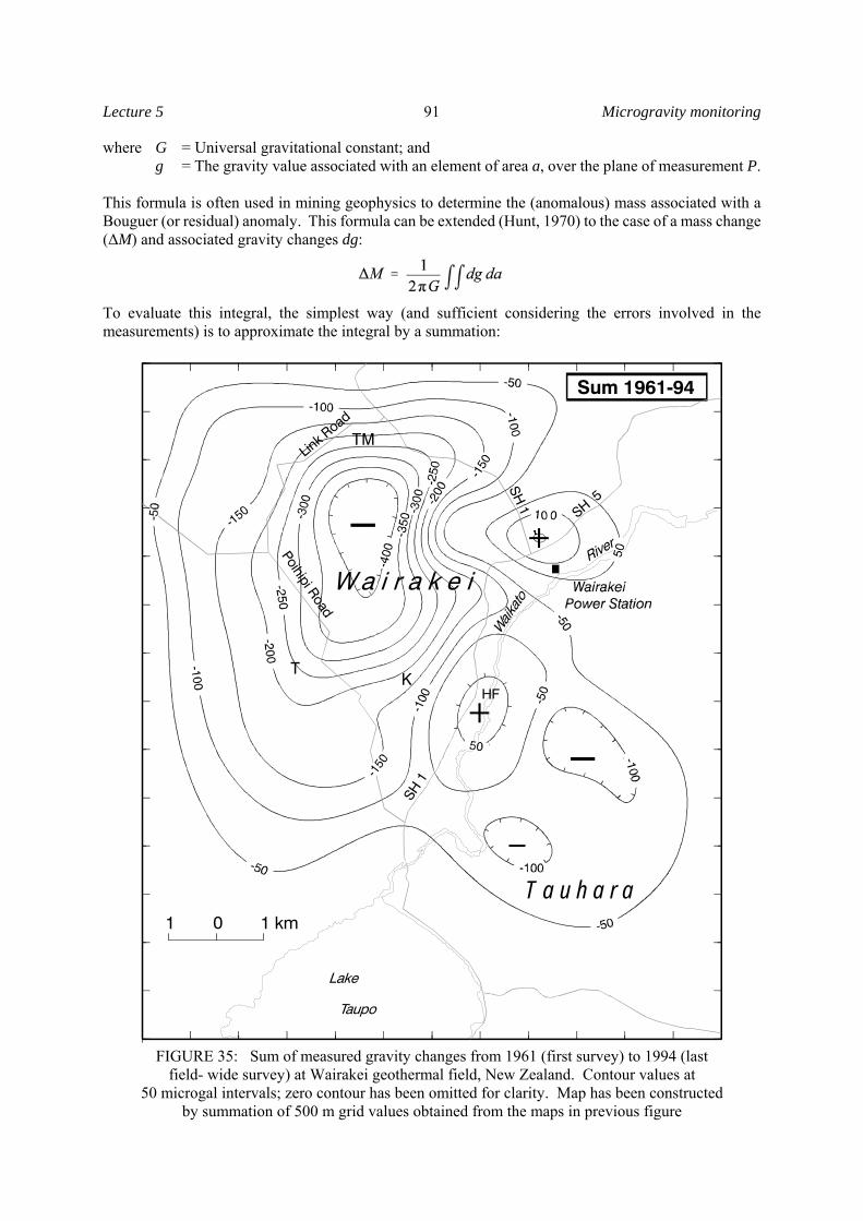
Lecture 5 Microgravity monitoring91
01 1 km
Poihipi Road
_
_
_
+
+
Taupo
Lake
SH 1
SH 5
Waik
ato
River
SH 1
K
TM
T
HF
Sum 1961-94
T a u h a r a
W a i r a k e i
Link R
oad
FIGURE 35: Sum of measured gravity changes from 1961 (first survey) to 1994 (lastfield- wide survey) at Wairakei geothermal field, New Zealand. Contour values at
50 microgal intervals; zero contour has been omitted for clarity. Map has been constructedby summation of 500 m grid values obtained from the maps in previous figure
where G = Universal gravitational constant; andg = The gravity value associated with an element of area a, over the plane of measurement P.
This formula is often used in mining geophysics to determine the (anomalous) mass associated with aBouguer (or residual) anomaly. This formula can be extended (Hunt, 1970) to the case of a mass change(ΔM) and associated gravity changes dg:
To evaluate this integral, the simplest way (and sufficient considering the errors involved in themeasurements) is to approximate the integral by a summation:

Microgravity monitoring Lecture 592
where Δg = Average gravity change in a small element of an area Δa, and the summation is extendedover a wide area.
In practice, the summation can be made numerically using a computer program, or more commonly bygridding the gravity change map, estimating the average gravity change in each grid square, and summingthese values to obtain G ΔgΔa. In doing this it is important that the gravity data extends well beyond theregion of measurable gravity changes associated with the field, and the area of each element is sufficientlysmall that the error in the estimate of Δg in the element is about the same as that of the measurement (andcontouring) of Δg.
The value of ΔM obtained is the net mass loss/gain for the whole field for the period between the gravitysurveys. This method of determining the mass change is very powerful because it is completelyindependent of any assumptions about fluid density, depth of production, permeability, or porosity. Itsaccuracy is limited only by the precision of the gravity measurements, and errors inherent in contouringand summing the data.
If the amount of mass withdrawn from the field by the wells (Mw), and any natural loss from surfacedischarge features (Mt) is known then the overall amount of mass recharge (R) can be determined
During production, the mass withdrawn by the wells is usually much greater than that lost from the surfacefeatures, however the latter needs to be monitored because it may change with time. For example, atWairakei natural loss before production was about 13 Mt/yr, but after 20 years of production haddecreased to about 6 Mt/yr. Values for mass discharge and recharge for Wairakei, calculated bysummation of the gravity changes, are given in Table 6 and have an estimated uncertainty of about 15%.
TABLE 6: Mass discharge and recharge values for Wairakei, MB is the mass withdrawn (Mt),MN the natural mass discharged, MT the total mass loss (MB+MN) is the integrated sum of gravity
changes (N m2/kg), MC the net mass change (Mt), and MR the mass recharge (Mt) (Hunt, 1995)
Period MB MN MT IS MC MR1950-611961-671967-741974-831983-91
145360400390375
12555604540
270415460435415
na-71-130
+19
-100?-235-350
+45
170180425435460
9.3 Testing numerical reservoir simulation models
Gravity change data can be used to discriminate between two (or more) numerical reservoir simulationmodels for exploitation of a field. The models predict development of a 2-phase zone and subsequentchanges in saturation which involve assumptions about the geometry of the field, various reservoirproperties, and behaviour of the field during exploitation. The models are generally developedprogressively.
Prior to production, little information is available about response of the field to exploitation and generallyonly that resulting from test discharges can be used to set up the models. Under such circumstances it islikely that several different models can be devised which fit the data. If there has been sufficient masswithdrawal to cause gravity changes during the pre-production period it may be possible to test the modelsby calculating the predicted gravity effects and comparing them with measured gravity changes.

Lecture 5 Microgravity monitoring93
Discrepancies between the theoretical (model-derived) and measured gravity changes may indicate thatassumptions made in setting up the models are wrong. Comparison of the theoretical and measuredgravity changes should focus on the lateral extent and amplitude of the gravity changes. Large measuredchanges at points further away from the test discharge area may indicate values assumed (in the model)for permeability are too low, or for porosity are too high. This application of the microgravity techniquemay be particularly useful in the situation where the test wells are confined to a small part of the field.
The most favourable situation is where there is a period of field-wide test discharge, followed by a period ofno (or limited) discharge so that any recovery can be monitored. Several gravity surveys during the dischargeand recovery periods may provide sufficient information for discrimination between different simulationmodels. However, it should be recognised that the gravity changes are likely to be much smaller than thosewhich may occur during the production period and consequently the precision of the gravity surveys, mayneed to be greater than for later surveys. This, in turn, may necessitate using fewer survey points, carefullychosen to maximise discrimination between the models. Natural discharges may be greater than the testdischarges, and so need to be known accurately.
The technique was used to test initial models for the Broadlands (Ohaaki) field. It was found that changes invapour saturation in the test discharge area were over-estimated, and their lateral extent was under-estimated(Hunt et al., 1990a). This led to the conclusion that the upper part of the production zone may be shallower,thinner, have greater porosity, and extend further than considered in the initial models.
9.4 Determination of saturation changes
Liquid saturation changes in a 2-phase zone as a result of boiling (dry out) or cooling and condensationduring production can be determined for areas of the field if other variables (temperature change, liquiddrawdown, and thickness) are known using the following basic 1-d equation:
However, saturation changes are best determined by using numerical reservoir simulation models, andvarying the saturation change in appropriate blocks, until a match is obtained between the calculated andobserved gravity changes.
9.5 Tracking the path of reinjected fluid
Reinjection involves the continuous transfer of waste liquid, generally back into the reservoir, and usuallyinto a different part of the field from where it was withdrawn (production area). There is thus a transferof mass from one place to another, and hence we might expect to observe a gravity increase in the vicinityof the reinjection wells. However, experience (tracer tests, pressure and temperature measurements)suggests that the reinjected liquid rarely remains in the vicinity of the reinjection wells. There are manyscenarios for what happens to the reinjected fluid. Taking two simple cases:
1. Reinjection into the 2-phase zoneThe liquid is cooler and hence denser than the liquid present, and tends to sink towards the bottomof the zone. The process is complex: the cooler liquid will cause steam to condense, thus increasingthe saturation in pores. Generally the rocks do not have isotropic permeability and so the liquid willmove more rapidly along paths of high permeability and in response to any pressure gradients thatmight be present.
The pattern of gravity increases associated with this process will therefore generally be non-uniform,and will reflect the directions of increased permeability and/or pressure gradients. Furthermore, byexamination, and quantitative analysis of the gravity data from several repeat surveys it may be

Microgravity monitoring Lecture 594
possible to determine the rate of flow of the reinjected fluid in particular directions. While thereinjected liquid remains in the 2-phase zone there will be a relatively large gravity signal because theliquid will be replacing vapour in the pores or fractures and hence there will be a large density change.
2. Reinjection into the deep-liquid zoneReinjection of relatively cool liquid into a hot, single-phase (liquid) zone beneath a 2-phase zone ismore complex, and the effects will depend on the depth of reinjection below the deep-liquid level, thepermeability (both vertical and horizontal) of the rocks, and the pumping pressure. Two extremesituations are:
(a) The depth of reinjection is well below the deep-liquid level and vertical permeability is low. Thereinjected liquid then flows out of the reinjection wells and displaces pore liquid horizontally.Although the reinjected fluid is cooler and hence denser than the displaced liquid, the densitychange is unlikely to be large enough to cause significant gravity changes at the surface. Forexample: if the reinjected water has a temperature of 150°C and completely displaces water at250°C in the pores of a rock with porosity 0.3, then the density change is (917 - 799) × 0.3 = 35kg/m3. Compare this with 150°C water displacing a similar volume of steam at 250°C: (917 -19) × 0.3 = 269 kg/m3.
Liquid water is (in this situation) incompressible, and so the displaced water must go somewhere.The most likely place for it to move to is laterally into the 2-phase zone; i.e. it will cause a lateralmovement of the boundary of the 2-phase zone, some distance from the reinjection wells. At thispoint, liquid will replace steam in the pores and there will be a significant gravity change signalat the surface. The amplitude of the gravity changes will depend not only on the geometricsituation, but also on what other changes are occurring in the reservoir in the vicinity of the 2-phase/1-phase boundary. However, the presence of localised gravity increases adjacent to (butnot in) a reinjection area might signal the lateral flow of reinjected fluid from the reinjection wellsto that point. Movement of such local gravity increases, between successive surveys, will reflectthe direction of movement of the reinjected fluid.
(b) The depth of reinjection is below the deep liquid level, and vertical permeability is relatively high.In this case the reinjected fluid will displace pore liquid vertically and the deep-liquid level willbe displaced upwards in a cone of impression (this is the reverse of a cone of impressioncommonly found in groundwater surfaces around a pumped well). Generally the permeabilityof the rocks in and around the reinjection area will be anisotropic, and so the reinjected fluid willnot flow symmetrically out from the reinjection area. This permeability anisotropy will cause thecone of impression to be similarly asymmetrical, indicating directions of greater and lesserpermeability. At Wairakei, a cone of impression formed by such reinjection, was crescent-shaped, indicating increased flow in two, near-perpendicular directions (Hunt et al., 1990b).
3. Injection outside the fieldIf the liquid is injected into or outside the field boundary then the liquid may not interact with thegeothermal system. The ability for significant amounts of fluid to be injected outside the fieldindicates the presence of porous formations capable of absorbing the liquid. Such formations arelikely to be highly porous and have low saturation; the injected fluid will replace air in the intersticesand hence there will be a large density change (even neglecting cooling effects). Gravity changes(increases) in the vicinity of the reinjection area will therefore indicate the presence (location) ofinjected liquid, and changes in location between successive surveys will indicate migration of theinjected liquid.
In the above cases, note that as the plume of injected fluid moves, the gravity changes will be associatedonly with the pores that have been saturated since the last survey; in previously saturated pores there willbe no significant density change and hence no gravity change.

Lecture 5 Microgravity monitoring95
Quantitative analysis of the gravity data can be made using standard 3-d gravity modelling programs,provided values are known (or can be assumed) for: porosity, initial saturation, liquid density, and thegeometry of the situation (depth or initial position of deep liquid level).
9.6 Determination of reservoir properties
Exploitation of a liquid-dominated geothermal system generally results in a transfer of mass (from onepart of the field to another), which may cause measurable gravity changes. In some cases, the rate of masstransfer is controlled by the properties of the rock in the reservoir (e.g. permeability), hence the rate ofgravity change with time is related to those properties. In such cases values for the properties can bedetermined from repeat microgravity measurements using numerical reservoir simulation models. Twosuch cases are the following:
1. During formation and expansion of a 2-phase zone in the initial stages of productionAnalysis of gravity changes at Wairakei geothermal field using simple radially symmetrical modelsand the MULKOM simulator showed that, for survey points near the centre of the production area,the size of theoretical changes soon (< 3 years) differs greatly (> 50 microgal) for different values ofpermeability (Hunt and Kissling, 1994). For example, after only 12 months the gravity change in thecentre of the borefield is predicted to be -330 microgal for a permeability of 50 md and -180 microgalfor a permeability of 200 md. Good estimates of permeability may be obtained by comparing themeasured gravity changes with theoretical curves of gravity change calculated for differentpermeabilities, using a simple plot of gravity change against time. The analysis for Wairakeisuggested that the gravity changes are most sensitive to differences in reservoir permeability at pointsclose (< 1 km) to the production area (i.e. area of greatest liquid drawdown), but elsewhere are moremodel dependent (in particular to radius of the model). Application of this technique thereforedepends on sufficient information being available to construct a realistic numerical simulation model,and a simulator which can generate theoretical gravity changes.
2. During reinjection which causes displacement of the deep liquid levelAs outlined above, reinjection may cause displacement of the deep-liquid level (vertically or laterally).Taking the case of vertical upward displacement of the deep liquid level, the shape of the cone ofimpression and its rate of growth (or decay, if reinjection stops) is controlled by the permeability ofthe rocks in that area. Note that the gravity signal reflects mainly the resaturation of the pores in the2-phase zone; the effect of mass increase due to the denser (cooler) reinjected water at depth is small.By measuring the rate of change of size and shape of the cone of impression from several gravitysurveys, and modelling this using a numerical simulator in which the permeability is adjusted untilthe measured and calculated gravity changes are in agreement, values for permeability (vertical,horizontal) can be determined. If the horizontal permeability is anisotropic, values for permeabilityin different directions may be calculated. Successful application of this technique will depend on theavailability of adequate gravity change data in the vicinity of the reinjection well(s), including oneor more baseline surveys to enable corrections to be made for other (more extensive) changes thatmight be occurring (such as a general rise or fall in the deep liquid level).
This technique was used at Wairakei during a reinjection test into an older part of the borefield. Usingan analytical model (Theis or line source solution), values of 18.2 and 5.4 dm were obtained forpermeability-thickness (kh) assuming anisotropic permeability (Hunt and Kissling, 1994). The modellingalso provided a value of 8.7 × 10⁻⁶ m/Pa for storativity (nch).

Microgravity monitoring Lecture 596
10. CASE HISTORIES
Microgravity surveys have been made at more than 10 producing geothermal fields: Wairakei, Ohaakiand Kawerau in New Zealand; Bulalo, Tiwi, and Tongonan in the Philippines; Larderello and Travale inItaly; Hatchobaru, Takigami and Yanaizu in Japan. They have also been tried at The Geysers and Heberfields in USA, and at Cerro Prieto in Mexico, but apparently abandoned due to political considerationsand lack of funding. It is rumoured that they have also been made in some other fields, but abandonedfor a variety of reasons (chiefly poor measurement techniques and failure to install adequate survey marks)which have resulted in spurious results when the gravity changes between the first and second surveyshave been calculated. However, this is exactly what happened at Wairakei in the early 1960s (Hunt,1995), and it should not discourage use of the technique.
10.1 Wairakei (New Zealand)
Wairakei is a liquid-dominated field, located in the central part of the North Island. Test drilling beganin 1950, and commissioning of the power station began in 1958 and continued until 1962, at which timethe installed capacity was 193 MW (gross). There has been no significant reinjection; all waste water isdischarged into the nearby Waikato River.
The technique of using repeat microgravity measurements to investigate the effects of exploitation of ageothermal field was developed using data from Wairakei. During nearly 40 years of production, 13repeat surveys have been made. The first survey, however, was not made until 1961 (3 years afterproduction began), and although carefully made, was not done to the now accepted requirements ofprecision or redundancy. Furthermore, few measurements of elevation or groundwater level change weremade at that time. However, by the early 1970s significant improvements in gravity measurement andreduction techniques had been made, and monitoring programmes had been implemented. Earlyinterpretations of the gravity change data clearly showed that the largest changes occurred during the earlystages of development of the field and that during this time there was little natural recharge of fluid - thereservoir was being mined of fluid. The results of the 1961-67 and 1967-74 survey periods (Figure 34)showed the necessity for a comprehensive baseline survey to be made before production began. Duringthe early 1980s, the microgravity results obtained at Wairakei, in conjunction with the reservoirengineering data enabled the various causes of gravity changes to be understood (Allis and Hunt, 1986).
The largest gravity changes have been in the Eastern borefield which formed part of the main productionarea during the early stages of development. Between 1961 and 1974, gravity values decreased by up to560 microgal, but have subsequently increased by about 440 microgal (Figure 36). The decrease wascaused by expansion of the 2-phase zone and dry-out of the upper part of this zone which has becomevapour-dominated (Allis and Hunt, 1986). The subsequent increases have been attributed to re-saturationof the lower part of the 2-phase zone by downflows of cold groundwater; i.e. the deep liquid level hasrisen. In the late 1980s, environmental concerns necessitated a study of reinjection and a long-term (13-month) test was undertaken during 1988-89 in part of the borefield which had the greatest pressuredecrease. Initial theoretical calculations suggested that there might be little gravity change associated withthe reinjection and so a full study was not undertaken; instead gravity measurements were made onlybefore and immediately after the test, and not during the test. This proved to be a mistake. There was asignificant gravity change (+120 microgal) associated with the reinjection which on analysis showed thatthe reinjected fluid had flowed in two directions away from the reinjection bore (Hunt et al., 1990b). Thisled to an improved understanding of some of the physical processes involved in the 2-phase zone, and therealisation that in certain (but not unusual) circumstances the gravity changes could be related to physicalproperties of the reservoir and in particular permeability-thickness (kh) and storativity (φch) (Hunt andKissling, 1994). If a more detailed gravity monitoring programme had been undertaken it might havebeen possible to better determine anisotropic values for kh. The results of the surveys during thereinjection trial also led to the concept that the permeability could be determined from gravity

Lecture 5 Microgravity monitoring97
50 55 60 65 70 75 80 85 90 95Year
-600
-500
-400
-300
-200
-100
0
100G
ravi
ty C
hang
e (m
icro
gal)
A97
AA77 (Karapiti)
AA13_
_ _
_ _
_ _
_ _
_ _
_ _ ProductionTesting
effect ofreinjection test
_
_ _ _
_ _
FIGURE 36: Gravity changes at selected benchmarks in Wairakei geothermal field,New Zealand. Benchmarks AA13 and A97 are in the Eastern borefield. Note the gravitydecreases during the early stages of production as the 2-phase zone expanded, followedby the gravity increases as the deep water level in the Eastern borefield rose as the rocks
became re-saturated as a result of cold downflows
measurements during the early stages of expansion of the 2-phase zone. Unfortunately, insufficientmeasurements had been made during these stages at Wairakei or Ohaaki fields; one measurement atWairakei indicated a permeability of 100 md (Hunt and Kissling, 1994). We must now wait for sufficientmeasurements to be made in another field to fully test this concept.
10.2 Ohaaki (New Zealand)
Ohaaki (Broadlands) is a liquid-dominated field, situated 25 km north-east of Wairakei. Development ofthe field was unusual; a 4 year period (1967-1971) of large-scale test discharges (without reinjection) wasfollowed by 16 years (1972-1988) of relatively minor discharges which allowed recovery of the field,before full-scale production (and reinjection) for a 116 MW (gross) power station was started in 1988.During the test discharge period deep-liquid pressures decreased by about 15 bar, but subsequentlyrecovered by about 10 bar during the recovery period, before decreasing again when production began.
Seven, field-wide gravity surveys have been completed to date which span the test discharge, recoveryand production periods. Gravity changes (max. -165 microgal) during the test discharge showed that therewas little or no recharge during this period, and the field was effectively mined (Hunt, 1987). During therecovery period there were positive gravity changes within the field (up to +65 microgal) which indicatethat natural recharge exceeded the small amount of mass withdrawn. Gravity change data for thedrawdown and recovery periods were used to test 3 numerical reservoir simulation models for the fieldprior to production beginning (Hunt et al., 1990a). The models predicted changes in vapour (or liquid)saturation with time, and hence changes in density from which changes in gravity could be easilycalculated. The results showed that none of the models adequately explained the microgravity data,suggesting that the upper part of production zone was shallower, thinner, had greater porosity, andextended further than considered by the models. This allowed the models to be refined before productionbegan.
Since production began, large gravity changes (up to -200 microgal) have occurred in the central part ofthe field. The distribution of negative gravity changes within the field is similar to the temperature

Microgravity monitoring Lecture 598
65 70 75 80 85 90 95Year
-350
-300
-250
-200
-150
-100
-50
0G
ravi
ty C
hang
e (m
icro
gal)
-25
-20
-15
-10
-5
0Pressure C
hange (bar)
H339 (Western SF)
H304 (Outside field)
Pressure
FIGURE 37: Gravity changes at benchmarks inside and outside the Ohaaki geothermal field.Note how the gravity changes at benchmark H339 (near centre of Western steamfield)
follow the reservoir pressure changes
FIGURE 38: Block diagram summarising masschanges in the Ohaaki field during 1989-96,determined from microgravity measurements
distribution at depth, and probably reflectsmainly the extension (both horizontally andvertically) of the 2-phase zone in the reservoir,and reduction in saturation (dry-out) within thiszone. This explanation is consistent with thegravity changes at benchmarks in the area ofgreatest change, which follow the trend in deep-liquid pressure declines in the production area(Figure 37). Despite 70 Mt having beenreinjected around the edges of the field therehave been no positive gravity changes in theseareas indicating that the reinjected water haslaterally displaced fluid near the reinjectionwells. Analysis of the data (Hunt, 1997)indicates that natural recharge has been onlyabout 5 Mt of the 31 Mt mass lost to theatmosphere (Figure 38).
10.3 Tongonan (Philippines)
This is a large, liquid-dominated field, located inLeyte Island. Development began in 1983 withthe commissioning of a 37.5 M power station(Tongonan I). Since then a further 118 MW (Upper Mahio, in 1996) and 77 MW (Malitbog) have beenadded. Annual withdrawal rates increased from 5 Mt/yr in 1983 to 15.8 Mt/yr in 1994. By March 1995,a cumulative total of 131 Mt had been withdrawn of which 62 Mt had been reinjected.
Five microgravity surveys have been conducted (1980, 1981, 1982, 1985, 1995) at about 100 surveypoints. The most extensive and reliable data are for the 1981 and 1995 surveys. Erroneous levelling dataprecluded the interpretation of 1981-95 data, but if there was no ground subsidence then the gravitychanges have been less than 50 microgal over all the field except in the Mahio area where changes of upto -75 microgal were measured (Apuada & Hunt, 1996).
Lecture 5 Microgravity monitoring99
10.4 Bulalo (Philippines)
Bulalo is a liquid-dominated field, located 70 km south-east of Manila. Production began in 1979 withan installed capacity of 110 MW, increased to 220 MW in 1980, 330 MW in 1984 and 426 MW in1996.
Fieldwide gravity and levelling surveys have been conducted every 1-3 years since 1980, and cover anarea of about 36 km2. The gravity measurements were initially made at 87 benchmarks, and the networkhas subsequently been increased to 120 measurement points (San Andres and Pedersen, 1993; Protacioet al., 2000). Bi-monthly gravity monitoring at six stations (1986-1987) indicated that the uncertainty dueto non-reservoir causes is ±20 microgal, which is attributed to variations in rainfall and groundwater level.Surveys were usually conducted during the dry months of March, April and May to minimise the effectsof rainfall. Selected benchmarks (up to 7 km from the centre of production) were used as fixed referencesfor datum shift (base change) adjustments. Ground subsidence of up to 0.5 m has occurred, centred onthe production area.
Between 1980 and 1991, gravity changes exceeded -250 microgal, and the maximum rate of change was-26 microgal/yr at a point near the centre of production. The cumulative gravity changes (1980-1999)have now reached almost –600 microgal in the central part of the production area. This sector has highexcess steam indicating widespread on-going change from brine to steam. The smallest cumulativechange in the production area is now more than –250 microgal. The gravity decreases within theproduction area have been near-uniform with time.
Mass discharges predicted by recent reservoir simulation modelling have generally matched those inferredfrom the observed gravity data. According to simulation studies, no recharge occurred between 1980 and1984. The mass recharge between 1984 and 1991 was estimated to be 30% of net fluid withdrawal duringthe same period, equivalent to an average rate of 175 kg/s (630 t/hr). Calculations indicate that there hasbeen about 42% recharge of the 374 Mt net mass loss since 1980 (Protacio et al., 2000).
10.5 Tiwi (Philippines)
Tiwi is liquid-dominated field situated 250 km south-east of Manila. Production began in 1979 with aninstalled capacity of 110 MW which was raised to 220 MW in 1980 and then to 330 MW in 1982. Totalmass withdrawal peaked at about 38 Mt/yr in 1983, but by 1990 had fallen to 22 Mt/yr; reinjection beganin 1983 and from then until 1990 has been about 9 Mt/yr.
Microgravity surveys began in 1979, and subsequent surveys were made in 1980, 1982, 1984, 1986, 1988and 1990 (San Andres, 1992). Surveys have been made regularly since 1990 but the results have not beenpublished.
The gravity data (San Andres, 1992) delineated areas of decreasing gravity over the production area,which were caused mainly by development of a steam zone. Initially, large gravity decreases wereobserved in the eastern Naglagbong area which provided most of the geothermal production. At the sametime, significant gravity decreases also were observed in the Kap-Mat area in the west. This behaviouris consistent with a shallow hydraulic connection between these two areas. In the Kap-Mat area thegeneral trend in gravity has been linear rate of decrease with time, consistent with expansion of the steamzone and increasing in vapour saturation. The initial rapid gravity decline in Naglagbong from 1979 to1984 was followed by minor gravity decreases from 1984 to 1990 due to declining local production andcold water influx. Mass recharge at Tiwi was estimated to be a minimum of 50% of net withdrawalsbetween 1979 and 1990.
Microgravity monitoring Lecture 5100
10.6 Larderello (Italy)
Larderello was the first geothermal field to be commercially exploited: production began in 1921. Thefield is vapour-dominated. Total production is currently about 800 t/hr (7 Mt/yr) of which about 200 t/hr(1.8 Mt/yr) is reinjected.
Microgravity surveys began in 1986, and since then a further 5 surveys have been made: 1987, 1988,1989, 1991, 1993 (Dini et al., 1995). Gravity changes during the whole of this period have been verysmall. The largest changes have been similar to the "environmental noise" (15 microgal), indicating therehas been almost complete mass recharge. Consistent, positive gravity changes in the main reinjectionarea, however, suggest that some of the reinjected water is being accumulated.
10.7 Travale-Radicondoli (Italy)
Travale field is located about 15 km southeast of Larderello. It is also a vapour-dominated geothermalsystem, and the average production rate is 100 kg/s (3.15 Mt/yr). Reinjection is insignificant.
Microgravity measurements were first made in 1979, and since then 7 further surveys have been made.Only small (<30 microgal) gravity changes have been measured. Analysis of the data shows about 97%of the fluid withdrawn between 1979 and 1991 has been replaced, indicating that (for this period of time)the field has been in a quasi-equilibrium state with respect to mass changes ( di Filippo et al., 1995).
10.8 The Geysers (United States of America)
The Geysers is a vapour-dominated field, located in northern California, and is the largest field in theworld both with respect to lateral extent and power produced. Production began in 1960 with an 11 MWplant and by 1993 the field was producing 1193 MW, however, since the late 1980s there has beenconsiderable decline in the supply of steam. Information about the field has been restricted by commercialconfidentiality, but Denlinger et al. (1981) state that between 1974 and 1981 about 20% of the masswithdrawn was reinjected, and the net mass produced was about 26 Mt/yr.
Microgravity measurements were made in 1974, and repeated in 1977. The maximum gravity change was-120 microgal, near the centre of the production region, and analysis suggested that recharge was small(Isherwood, 1977). The data was also analysed by Allis (1982) who showed that the ratio of gravitychange to ground subsidence may be a useful indicator of the rate of fluid depletion in vapour-dominatedsystems because it was independent of reservoir thickness, pressure drop, and porosity. The ratio for thatpart of the field with greatest production was about -14 microgal/cm corresponding to a recharge of about55%, but in some parts of the field the recharge was less than 25%. No published reports of gravitychange measurements have been made after 1977, except for a brief (38 day) test of a cryogenicgravimeter in 1979 (Olson and Warburton, 1979). However, calculations (Allis et al., 2000) suggest thatthere will have been an average gravity decrease of up to 60 microgal/y, peaking about 1987, and thecumulative gravity change at The Geysers has been about 1000 microgal.
Recently, injection of water from outside the field has begun at several places in the field: the SoutheastGeysers Effluent Pipeline project (SEGEP). Calculations (Allis et al., 2000) show that the gravity effectsof this reinjection will be in the range 1-4 microgal year, and microgravity measurements may be usefulin tracking the path of the injected water.

Lecture 5 Microgravity monitoring101
10.9 Cerro Prieto (Mexico)
Cerro Prieto is a liquid-dominated field situated in the north-western part of Mexico. Production beganin 1973 with an output of about 69 MWe, which has been progressively increased to about 570 MWe in1995.
Microgravity measurements of 70 survey points were started in 1978, and repeat surveys were madeannually until 1983 (Grannell et al., 1984) but no significant results have been reported and it is believedthe measurement programme ceased in 1983.
10.10 Hatchobaru (Japan)
Hatchobaru is a liquid-dominated field, situated in central Kyushu. A 55 MW power station was openedin June 1977 (No. 1 unit) and a further 55 MW added in June 1990 (No. 2 unit). The combined productionrate is now about 1325 t/hr of liquid and 590 t/hr steam; there are 21 production and 10 reinjection wellsin use. The main production is from depths of 1-2.5 km, and reinjection is at depths of 1-1.5 km.
Nineteen microgravity surveys, involving 44 survey points, have been made between 1990 and 1997 (Eharaet al., 1997; Nishijima et al., 2000). Gravity decreases of up to 250 microgal have been measured in theproduction area. In the reinjection area, gravity values at one point increased rapidly by up to about +80microgal, and have since gradually decreased. Mass changes, calculated by integrating the gravity changes,suggest that between 1991 and 1993 of 32.4 Mt withdrawn, 16.7 Mt was discharged to the atmosphere, 15.7was reinjected and about 16.3 Mt of natural recharge occurred (Nishijima et al., 2000).
10.11 Takigami (Japan)
Takigami is a liquid-dominated field, situated in Kyushu. A 25 MW power station began production inNovember 1996; there are 4 production and 9 reinjection wells.
Eleven microgravity surveys were conducted between May 1991 and March 1993 (Ehara et al., 1995); thesesurveys span a 4 month period of pre-production and reinjection testing (3 Mt withdrawn, 2 Mt reinjected)conducted between November 1991 and February 1992. Gravity changes of up to -150 microgal weremeasured, but most of the changes were found to be due to large seasonal variations in shallow groundwaterlevel. Takigami lies in a mountainous area with an annual rainfall of 2.6 m, most of which occurs in thesummer months. After correction for the gravity effects of these variations, gravity changes of up to +30microgal were determined for the reinjection area and up to -40 microgals in the production area (Ehara et al.,1994, 1995).
Since then, efforts have concentrated on better determination of the correction for groundwater level changesusing a multivariate regression model (Nishijima et al., 1999; Fujimitsu et al., 2000). A comparison betweenprecipitation and gravity shows that there are phase lags of 3-8 months between rainfall and groundwater levelchanges. The accuracy of the gravity changes obtained after removal of the groundwater changes determinedin this manner is estimated to be 10 microgal. Published data (Fujimitsu et al., 2000) show that in theproduction area there were gravity decreases of up to 30 microgal immediately prior to production (1995-1996), and increases of up to 40 microgal after production (1996-1997). There appears to have been no gravitychanges in the reinjection area since production began.
10.12 Yanaizu-Nishiyama (Japan)
Yanaizu - Nishiyama is a liquid-dominated field, situated in central Honshu. A 65 MW power station wascommissioned in May 1995. The production rate is 71 t/hr water and 525 t/hr steam from 15 deep wells (1.56-

Microgravity monitoring Lecture 5102
2.70 km). There are 3 reinjection wells (1.5 km deep).
Microgravity measurements were started at 83 survey points in September 1994; annual surveys have beenconducted since then and the survey network expanded to 138 points (Takemura et al., 2000). Since 1998,monitoring surveys have been carried out three times a year to determine if seasonal gravity variations occur.Near one gravity station, a weather monitoring station and soil moisture measuring equipment have beeninstalled. At the weather station, barometric pressure, air temperature and rainfall are measured at 30 min.intervals. Shallow groundwater monitoring wells have been installed adjacent to 10 gravity survey points, andchanges in water level monitored at 30 min. intervals.
11. LESSONS LEARNED
Microgravity measurements began at Wairakei geothermal field nearly 40 years ago, and since then thetechniques of measurement and interpretation have been developed, and we have learned:
1. It is important that a good baseline data set is obtained before exploitation begins.
2. The gravity surveys need to be accompanied by surveys to monitor ground subsidence and groundwaterlevel changes.
3. The measurement points need to extend well beyond the field boundaries to locate areas where reinjectedfluid may be going, to determine the significance level of the measurements, and to check that gravitychanges have not occurred at the base station.
4. The largest gravity changes occur in the early stages of exploitation and are associated with developmentof a two-phase zone: surveys at this time need to be more frequent.
5. The greatest benefits are achieved when the gravity change data are used in conjunction with numericalreservoir simulation models.
6. Predictions (of gravity change) are often wrong, and should be treated only as a rough guide to planningthe microgravity surveys.
7. We have never regretted obtaining more (extra) microgravity data; we have often regretted not takingmore. It is not possible to go back in time to collect extra data.
12. FUTURE TRENDS
Although the microgravity technique has been well developed over the last decade, some improvements canstill be made. The following are suggestions of what can be done.
12.1 Determination of the effects of groundwater and soil moisture variations
At present few studies have been made of the gravity effects of changes in shallow groundwater level andchanges in saturation in the Vadose zone. In porous formations, such as occur near the surface in activevolcanic regions, variations of several metres can cause gravity changes of about 10 microgal/m ofgroundwater level change. Seasonal variations in water storage in the Vadose Zone are also likely to beimportant; changes of about 12 microgal have been recorded in Finland (Makinen and Tattari, 1991).

Lecture 5 Microgravity monitoring103
12.2 Improvements in measuring and determining the effects of ground subsidence
In some fields, such as Wairakei and Ohaaki, significant ground subsidence has occurred as a result of pressuredrawdown in the reservoir and needs to be corrected for in determining gravity changes associated with massvariations in the reservoir.
Values for subsidence at the survey marks are usually obtained by optical levelling surveys; generally to 2nd
order standard. This traditional technique is time-consuming and therefore costly. New techniques areemerging which may replace optical levelling; these include (differential) GPS surveys (Nunnari andPuglisi,1994) and Synthetic Aperture Radar interferometry (Massonnet et al., 1997). At present these methodscannot provide the required precision quicker than optical levelling, except in regions of high topographicalrelief and poor access, but it is anticipated that improvements will occur in the near future.
To obtain an accurate correction for the gravity effect of subsidence it is also necessary to know the verticalgravity gradient at each survey mark. For some microgravity surveys the standard theoretical "free air"correction value of -308.6 microgal/m has been used for all measurements, and in other surveys an average ofseveral measured values has been used: -302 (±5) microgal/m for Wairakei and -295 (±8) microgal/m forOhaaki. Further studies are needed to measure and incorporate local variations of gradient into the calculationof the gravity effects of subsidence, and so reduce the uncertainty in the gravity change values.
12.3 Borehole gravimetry
Currently, all microgravity surveys in geothermal fields have been made at the ground surface, but theamplitude of the measured gravity changes would be greater if the measurements could be made closer to, orwithin, the regions of mass change. This has been suggested for monitoring depletion of hydrocarbonreservoirs (Schultz, 1989), however the temperature in geothermal wells is much higher than in oil and gaswells. Some borehole gravimeters (BHGM) have been developed for use in the mining and petroleum industry(Robbins, 1989; Popta et al., 1990), but currently the maximum environment temperature limit for suchinstruments is about 260°C, they require a 7 inch diameter hole, which must not deviate more than 14° fromthe vertical. Improvements in temperature limitations and reduction in the size of the instrument would berequired to make this technique feasible for geothermal field operation. In addition, a technique would needto be developed to ensure accurate repositioning of the meter in the hole in repeat surveys.

104
Hunt, T.M.: Five lectures on environmental effects of geothermal utilization Reports 2000 Number 1, 104-109
GEOTHERMAL TRAINING PROGRAMME
REFERENCES
Allis, R.G., 1981: Changes in heat flow associated with exploitation of the Wairakei geothermal field,New Zealand. NZ Journal of Geology & Geophysics, 24, 1-19.
Allis, R.G., 1982: Monitoring fluid depletion at The Geysers by the gravity change/subsidence ratio.Proceedings of the 8th Workshop on Geothermal Reservoir Engineering, Stanford University, Ca, 177-182.
Allis, R.G., 1990: Subsidence at Wairakei field. Geoth. Resourc. Counc., Trans., 14, 1081-1087.
Allis, R.G., 2000: Review of subsidence at Wairakei field, New Zealand. Geothermics, 29, 455-478.
Allis, R.G., Carey, B., Darby, D., Read, S. A. L., Rosenberg, M., and Wood, C.P., 1997: Subsidence atOhaaki field, New Zealand. Proceedings of the 19th New Zealand Geothermal Workshop, GeothermalInstitute, Auckland, 9-15.
Allis, R.G., Gettings, P., and Chapman, D.S., 2000: Precise gravimetry and geothermal reservoirmanagement. Proceedings of the 25th Workshop on Geothermal Reservoir Engineering, StanfordUniversity, Ca, 179-188.
Allis, R.G., and Hunt, T.M., 1986: Analysis of exploitation induced gravity changes at Wairakeigeothermal field. Geophysics, 51, 1647-1660.
Allis, R.G., and Zhan X., 2000: Predicting subsidence at Wairakei and Ohaaki geothermal fields, NewZealand. Geothermics, 29, 479-497.
Apuada, N., and Hunt, T.M., 1996: Microgravity measurements at Leyte geothermal power project. Paperpresented at 17th PNOC-EDC Geothermal Conference.
Armannsson, H., and Kristmannsdottir, H., 1993: Geothermal environmental impact. Geothermics, 21-5/6, 869-880.
Barbier, E., 1991: Geothermal energy: Its role in the generation of electricity and its environmentalimpact. In: “Electricity and Environment”. IAEA report, TECDOC-624, 163-176.
Bixley, P.F. 1990: Cold water invasion in producing liquid-dominated geothermal reservoirs.Proceedings of the 15th Workshop on Geothermal Reservoir Engineering, Stanford University, CA, 187-191.
Bixley, P.F., and Browne, P.R.L. 1988: Hydrothermal eruption potential in geothermal development.Proceedings of the 10th New Zealand Geothermal Workshop, Geothermal Institute, Auckland, 195-198.
Bixley, P.F., and Hattersley, D.S., 1983: Long term casing performance of Wairakei production wells.Proceedings of the 5th New Zealand Geothermal Workshop, Geothermal Institute, Auckland, 257-263.
Bolanos, G.T., and Parilla, E.V., 2000: Response of Bao-Banati thermal area to development of theTongonan geothermal field, Philippines. Geothermics, 29, 499-508.
Bonvalot, S., Diamont, M., and Gabalda, G., 1998: Continuous gravity recording with Scintrex CG-3Mmeters: a promising tool for monitoring active zones. Geophysal J. International, 135, 470-494.Bromley, C.J., and Mongillo, M.A., 1994: Hydrothermal eruptions - a hazard assessment. Proceedings

105Hunt References
of the 16th New Zealand Geothermal Workshop, Geothermal Institute, Auckland, 45-50.
Broucke, R.A., Zurn, W.E., and Slichter, L.B. 1982. Lunar tidal acceleration on a rigid Earth. AmericanGeophys. Union Geophysical Monograph, 16, 319-324.
Brown, L. 1993: New shorter Oxford English dictionary. Clarendon Press, Oxford.
Brown, K.L., 1995: Impacts on the physical environment. In: Brown, K.L. (convenor), Environmentalaspects of geothermal development. World Geothermal Congress 1995, IGA pre-congress course, Pisa,Italy, May 1995, 39-55.
Brown, K.L., Henley, R.W., Glover, R.B., Mroczek, E.K., and Plum, H., 1988: Dilution and boiling inthe Wairakei field due to exploitation 1959-1982. Proceedings of the 10th New Zealand GeothermalWorkshop, Geothermal Institute, Auckland, 263-268.
Budetta, G., and Carbone, D., 1997: Potential application of the Scintrex CG-3M gravimeter formonitoring volcanic activity: Results of field trials on Mt. Etna. J. Volcanology and Geotherm. Res. 76,199-214.
Clotworthy, A., Lovelock, B. and Carey, B., 1995: Operational history of the Ohaaki geothermal field,New Zealand. Proceedings of the World Geothermal Congress 1995, Florence, Italy, 3, 1797-1802.
Cody, A.D., and Lumb, J.T., 1992: Changes in thermal activity in the Rotorua geothermal field.Geothermics, 21. 215-230.
Denlinger, R.P., Isherwood, W.F., and Kovach, R.L., 1981: Geodetic analysis of reservoir depletion atThe Geysers steamfield in northern California. Journal of Geophysical Research, 86, 6091-6096
Di Filippo, M., Dini, I., Marson, I., Palmieri, F., Rossi, A., and Toro, B., 1995: Subsidence and gravitychanges induced by exploitation in the Travale-Radicondoli geothermal field (Tuscany, Italy).Proceedings of the World Geothermal Congress 1995, Florence, Italy, 3, 1945-1949.
Dini, I., Marson, I., Palmieri, F., and Rossi, A., 1995: Reinjection monitoring in the Larderellogeothermal field using microgravity and topographic measurements. Proceedings of the WorldGeothermal Congress 1995, Florence, Italy, 3, 1851-1854.
DiPippo, R., 1991: Geothermal energy: Electricity generation and environmental impact. Energy Policy,19, 798-807.
Driscoll, F.G., 1986: Groundwater and wells. Johnson Division, St. Paul, Minnesota, 1089 pp.
Ehara, S., Fujimitsu, Y., Motoyama, T., Akasaka, C., Furuya, S., Goto, H., and Motomatsu, T., 1995:Gravity monitoring of geothermal reservoirs - a case study of the production and reinjection test at theTakigami geothermal field, Central Kyushu, Japan. Proceedings of the World Geothermal Congress1995, Florence, Italy, 3, 1955-1958.
Ehara, S., Fujimitsu, Y., Nishijima, J., and Ono, A., 1997: Effects of development on geothermal systemsdeduced from gravity and thermal measurements: Japanese case studies. Proceedings NEDOInternational Geothermal Symposium 1997, 235-241.
Ehara, S., Motoyama, T., Akasaka, C., Furuya, S., Goto, H., and Motomatsu, T., 1994: Gravitymonitoring of geothermal reservoirs - a case study of the production and reinjection test at the Takigamigeothermal field, Central Kyushu, Japan. Journal of the Geothermal Research Society of Japan 16, 343-363 (in Japanese with English abstract and figure captions).
Ellis, A.J., and Mahon, W.A.J., 1977: Chemistry and geothermal systems. Academic Press, London, 392

106
pp.
ETSU, 1998: Environmental implications of renewable energy technologies. Draft report for IEARenewable Energy Working Party.
Fujimitsu, Y., Nishijima, J., Shimosako, N., Ehara, S., and Ikeda, K. 2000. Reservoir monitoring byrepeat gravity measurements at the Takigami geothermal field, Central Kyushu, Japan. Proceedings ofthe World Geothermal Congress 2000, Japan, 573-577.
Gabriel, A.K., Goldstein, R.M., and Zebker, H.A., 1989: Mapping small elevation changes over largeareas: Differential radar interferometry. J. Geophysical Research, 94, 9183-9191.
Glover, R.B., and Hunt, T.M., 1996: Precursory changes to natural thermal features during testing of theWairakei and Broadlands-Ohaaki fields. Proceedings of the 18th New Zealand Geothermal Workshop,Geothermal Institute, Auckland, 69-76.
Glover, R.B., Hunt, T.M., and Severne, C.M., 1996: Ohaaki Ngawha; Ohaaki Pool. Proceedings of the18th New Zealand Geothermal Workshop, Geothermal Institute, Auckland, 77-84.
Glover, R.B., Hunt, T.M., and Severne, C.M., 2000: Impacts of development on a natural thermal featureand their mitigation – Ohaaki Pool, New Zealand. Geothermics, 29, 509-523.
Glover, R.B., and Stewart, M.K., 1996: Chemical and isotopic changes in shallow groundwater causedby exploitation of the Wairakei geothermal field, New Zealand. Geothermics, 25, 647-661.
Goff, S., 2000: The effective use of environmental impact assessments (EIAs) for geothermaldevelopment projects. Proceedings of the World Geothermal Congress 2000, Japan, 597-603.
Goff, S., and Goff, F., 1997: Environmental impacts during development: Some examples from CentralAmerica. Proceedings of NEDO International Geothermal Symposium, 242-250.
Grannell, R.B., 1980: The use of surface gravity methods in monitoring subsurface reservoir changes,with case studies at Cerro Prieto, Mexico, and Heber, California. Geothermal Resources Council,Transactions 4, 49-52.
Hammer, S., 1945: Estimating ore masses in gravity prospecting. Geophysics, 10, 50-62.
Henley, R.W., Truesdell,A.H., and Barton, P.B., 1984: Fluid-mineral equilibria in hydrothermal systems.Society of Economic Geologists, Reviews in Economic Geology 1, 267 pp.
Hochstein, M.P., and Henrys, S., 1988: Assessment of total heat and mass transfer of a large pool usingthe balance method. Proceedings of the International Symposium on Geothermal Energy in Kumamotoand Beppu, Japan, Geothermal Research Society of Japan, 97-101.
Hunt, T.M., 1970: Gravity changes at Wairakei geothermal field, New Zealand. Geol. Soc. of America,Bulletin 81, 529-536.
Hunt, T.M., 1977: Recharge of water in Wairakei geothermal field determined from repeat gravitymeasurements. New Zealand Journal of Geology and Geophysics 20, 303-317.
Hunt, T.M., 1987: Recharge at Broadlands geothermal field 1967-1983 determined from repeat gravitymeasurements. D.S.I.R., Geophysics division, Wellington, New Zealand, report 216, 45 pp.
Hunt, T.M., 1988: Update on gravity changes in the main production borefield at Wairakei. Proceedingsof the 10th New Zealand Geothermal Workshop, Geothermal Institute, Auckland, 129-132.

107Hunt References
Hunt, T.M., 1995: Microgravity measurements at Wairakei geothermal field, New Zealand; a review of30 years data (1961-1991). Proceedings of the World Geothermal Congress 1995, Florence, Italy, 2,863-868.
Hunt, T.M., 1997: Microgravity changes during production from Ohaaki geothermal field, New Zealand.Geothermal Resource Council, Transactions 21, 191-195.
Hunt, T.M., Allis, R.G., Blakely, M.R., and O'Sullivan, M.J., 1990a: Testing reservoir simulation modelsfor the Broadlands geothermal field using precision gravity data. Geothermal Resources Council,Transactions 14, 1287-1294.
Hunt, T.M., Bixley, P.F., Carey, B.S., McCabe, W.M., and Young, R.M., 1990b: Results of a 13-monthreinjection test at Wairakei geothermal field, New Zealand. Geothermal Resources Council, Transactions14, 1193-1200.
Hunt, T.M., and Bromley, C.J., 2000: Some environmental changes resulting from development ofOhaaki geothermal field, New Zealand. Proceedings World Geothermal Congress 2000, Japan, 621-626.
Hunt, T.M., and Brown, K.L., 1996: Environmental effects of geothermal development andcountermeasures. Proceedings of the APEC Energy R&D and Technology Transfer and RenewableEnergy Resource Assessment Seminar, Beijing,6-9 February 1996, 243-255.
Hunt, T.M., and Glover, R.B., 1996: Environmental effects of mass withdrawal from liquid-dominatedgeothermal fields in New Zealand. Geoth. Resourc. Counc., Trans., 20, 213-220.
Hunt, T.M., and Kissling, W.M., 1994: Determination of reservoir properties at Wairakei geothermalfield using gravity change measurements. Journal of Volcanology and Geothermal Research 63, 129-143.
Hunt, T.M., Risk, G.F., and Bromley, C.J., 1998: History of geophysical studies at Wairakei.Proceedings of the 20th New Zealand Geothermal Workshop, Geothermal Institute, Auckland, 37-44.
Isherwood, W.F., 1977: Geothermal reservoir interpretation from change in gravity. Proceedings of the3rd Workshop on Geothermal Reservoir Engineering, Stanford University, Ca, 18-23.
La Fehr, T.R., 1965: The estimation of the total amount of anomalous mass by Gauss’s theorem. J.Geophys. Res., 69, 1911-1919.
Longman, I.M., 1959: Formulas for computing the tidal accelerations due to the sun and moon. J.Geophys. Res., 64, 2351-2355.
Luketina, K., 2000: New Zealand geothermal resource management – a regulatory perspective.Proceedings of the World Geothermal Congress 2000, Japan, 751-756.
Lund, J., 2000: World status of geothermal energy use, overview 1995-2000. Geothermics, 29, in press.
Makinen, J., and Tattari, S., 1991: The influence of variation in subsurface water storage on observedgravity. Proceedings 11th International Symposium on Earth Tides, 457-471.
Massonet, D. Holzer, T., and Vadon, H., 1997: Land subsidence caused by the East Mesa geothermalfield, California, observed using SAR interferometry. Geophysical Research Letters, 24, 901-904.
Melchior, P., 1983: The tides of the planet Earth. Pergamon Press, Oxford, 653 pp.
Mongillo, M.A., and Bromley, C.J., 1992: A helicopter-borne video thermal infrared survey of theRotorua geothermal field. Geothermics, 21, 197-214.

108
Nicholson, K., 1993: Geothermal Fluids; chemistry and exploration techniques. Springer Verlag, Berlin,263 pp.
Nishijima, J., Fujimitsu, Y., Ehara, S., and Motoyama, T., 2000: Reservoir monitoring by observationof gravity changes at some geothermal fields in Kyushu, Japan. Proceedings of the World GeothermalCongress 2000, Japan, 1515-1520.
Nishijima, J., Fujimitsu, Y., Ehara, S., Motoyama, T., and Simosako, N., 1999: Reservoir monitoring byobservation of gravity changes at the Takigami geothermal field, Central Kyushu, Japan. Geoth. Resourc.Counc., Trans., 23, 425-431.
Nunnari, G., and Puglisi, G., 1994: The global positioning system as a useful technique for measuringground deformations in volcanic areas. Journal of Volcanology and Geothermal Research, 61, 267-280.
O’Shaughnessy, B.W., 2000: Use of economic instruments in management of Rotorua geothermal field,New Zealand. Geothermics, 29, 539-556.
Olson, J.J., and Warburton, R.J., 1979: Continuous gravity observations at The Geysers: a preliminaryreport. Geothermal Resources Council, Transactions 3, 519-522.
Parker, S.P., 1980: Encyclopedia of environmental science (2nd edition). McGraw-Hill Book Company,NY, 858 pp.
Popta, J.V., Heywood, J.M.T., Adams, S.J., and Bostock, D.R.. 1990: Use of borehole gravimetry forreservoir characterisation and fluid saturation monitoring. Soc. Petrol. Eng., Technical Paper 20896.
Protacio, J.A. P., Golla, G.U., Nordquist, G.A., Acuna, J., and San Andres, R.B., 2000: Gravity andelevation changes at the Bulalo field, Philippines: independent checks and constraints on numericalsimulation. Proceedings of the 22nd New Zealand Geothermal Workshop, Geothermal Institute, Auckland,115-119.
Robbins, S.L., 1989: Borehole gravimetry reviews. U.S. Geological Survey, Circular 890, 9-19.
Rymer, H., 1989: A contribution to precision microgravity analysis using LaCoste and Romberg gravitymeters. Geophys. J. International, 97, 311-328.
San Andres, R.B., 1992: Precision gravity monitoring at the Tiwi geothermal field, Philippines. Proceeding of the 14th New Zealand Geothermal Workshop, University of Auckland, 189-194.
San Andres, R.B., and Pedersen, J.R., 1993: Monitoring the Bulalo geothermal reservoir, Philippines,using precision gravity data. Geothermics, 22, 395-402.
Schultz, A.K., 1989: Monitoring fluid movement with a borehole gravity meter. Geophysics, 54, 1267-1273.
Scott, B.J., Cody, A.D. 2000. Response of the Rotorua geothermal system to exploitation and varyingmanagement regimes. Geothermics, 29: 573-592.
Sherburn, S., Allis, R.G., and Clotworthy, A., 1990: Microseismic activity at Wairakei and Ohaakigeothermal fields. Proceedings of the 12th New Zealand Geothermal Workshop, Geothermal Institute,Auckland, 51-55.
Sherburn, S., Clotworthy, A., and Hunt, T.M., 1993: No induced seismic activity at Ohaaki geothermalfield. Proceedings of the 15th New Zealand Geothermal Workshop, Geothermal Institute, Auckland, 201-205.

109Hunt References
Şimşek, Ş., Günay, G., Elhatip, H., and Ekmekçi, M., 2000: Environmental protection of geothermalwaters and travertines at Pamukkale, Turkey. Geothermics, 29, 557-572.
Stark, M.A., 1990: Imaging injected water in The Geysers reservoir using microearthquake data. Geoth.Resourc. Counc., Trans., 14, 1697-1704.
Takemura, T., Shiga, N., Yokomoto, S., Saeki, K., and Yamanobe, H., 2000: Gravity monitoring inYanaizu-Nishiyama geothermal field, Japan. Proceedings of the World Geothermal Congress 2000,Japan, 2937-2941.
Thoreaux, H.D., 1860: Letter to Harrison Blake. Written 20th May, 1860.
Torge, W., 1989: Gravimetry. Walter de Gruyter, New York, 465 pp.
Webster, J.G., 1995: Chemical impacts of geothermal development. In: Brown, K.L. (convenor),Environmental aspects of geothermal development. World Geothermal Congress 1995, IGA pre-congress course, Pisa, Italy, May 1995, 79-95.
Webster J.G., and Timperley, M.H., 1995: Biological impacts of geothermal development. In: Brown,K.L. (convenor), Environmental aspects of geothermal development. World Geothermal Congress 1995,IGA pre-congress course, Pisa, Italy, May 1995, 97-117.