five lectures on translation surfaces …web.stanford.edu/~amwright/fivelectures.pdfother resources....
TRANSCRIPT

FIVE LECTURES ON TRANSLATION SURFACES ANDTHEIR ORBIT CLOSURES: AN INTRODUCTION FORGRADUATE STUDENTS IN ALGEBRAIC GEOMETRY
ALEX WRIGHT
Abstract. These are the notes for a five lecture course at theGraduate Workshop on Moduli of Curves, held July 7–18, 2014at the Simons Center in Stony Brook, NY, organized by SamuelGrushevsky, Robert Lazarsfeld, and Eduard Looijenga. Videos ofthe lectures are available online: lecture 1, lecture 2, lecture 3,lecture 4, lecture 5.
Familiarity with Riemann surfaces is assumed, but there are noother prerequisites to read these notes, either from dynamics oralgebraic geometry. The goal is to first illustrate the connectionsto special families of Riemann surfaces, and then to provide a firstintroduction to a subset of the most fundamental dynamical as-pects of the field. Each lecture includes a number of exercises, aswell as at least one accessible research problem.
Comments, corrections, and questions on these notes would bevery much appreciated, and can be sent to alexmurraywright@
gmail.com. If you are reading these notes and find a typo orunclear passage, please email me!
Contents
1. Translation surfaces 22. Affine invariant submanifolds 173. The action of GL+(2,R) 294. The straight line flow 405. Revisiting genus two with new tools 52References 61

2 WRIGHT
Acknowledgements: I am grateful to Ronen Mukamel for helpfulconversations that shaped the presentation of real multiplication ingenus 2, and to Preston Wake, Clark Butler, Elise Goujard, EmreSertoz, Paul Apisa, Ian Frankel, and Benjamin Dozier for finding typosand making helpful comments on these notes.
Other resources. There are a number of very good surveys ontranslation surfaces and related topics, for example [Esk06, For06a,HS06,Mas06,MT02,Mol13,Mol09,SW07,Via06,Yoc10,Yoc09,Yoc06,Zor06]. See here for a list with links to pdf files, compiled byLanneau. I primarily learned from the surveys [MT02,Zor06]
In addition to these surveys, the seminal paper [McM03a] of Mc-Mullen would be very good supplementary reading. It is availableonline here.
1. Translation surfaces
1.1. Equivalent definitions. This subsection has been written in afairly technical way, so that it may serve as a reference for anyonelooking for details on foundational issues. Most readers will want toskip some of the proofs on first reading. Anyone who already knowswhat a translation surface is can skip this subsection entirely.
In these notes, all Riemann surfaces will be assumed to be compactand connected. (A Riemann surface is a manifold of real dimension twowith an atlas of charts to C whose transition maps are biholomorphic.)Thus the term “Riemann surface” will be synonymous to “irreduciblesmooth projective algebraic curve over C.”
Definition 1.1. An Abelian differential ω on a Riemann surface X isa global section of the cotangent bundle of X. A translation surface(X,ω) is a nonzero Abelian differential ω on a Riemann surface X.
Thus “nonzero Abelian differential” and “translation surface” aresynonymous terms, but sometimes the notation is slightly different.Sometimes we might omit the word “translation,” and say “let (X,ω)be a surface” when we should say “let (X,ω) be a translation surface.”
The complex vector space of Abelian differentials on X will be de-noted H1,0(X). We assume the following facts are familiar to thereader.
Theorem 1.2. Let g denote the genus of X. Then dimCH1,0(X) = g.
If g > 0, each Abelian differential ω on X has 2g − 2 zeros, countedwith multiplicity.

FIVE LECTURES ON TRANSLATION SURFACES 3
Each nonzero Abelian differential is a 1-form, which is closed but notexact, and hence H1,0 is naturally a subspace of the first cohomologygroup H1(X,C) of X.
The following result is key to how most people think about transla-tion surfaces.
Proposition 1.3. Let (X,ω) be a translation surface. At any pointwhere ω is not zero, there is a local coordinate z for X in which ω = dz.At any point where ω has a zero of order k, there is a local coordinatez in which ω = zkdz.
Proof. We will work in a local coordinate w, and suppose that ω van-ishes to order k at w = 0. Thus we can write ω = wkg(w), where g issome holomorphic function with g(0) 6= 0. Note that∫ w
0
g(t)tkdt
vanishes to order k + 1 at 0, and thus admits a (k + 1)-st root. Definez by
zk+1 = (k + 1)
∫ w
0
g(t)tkdt.
By taking d of each side, we find zkdz = ω as desired. �
Let Σ ⊂ X denote the finite set of zeros of ω. At each point p0 ofX \Σ, we may pick a local coordinate z as above. This choice is uniqueif we require z(p0) = 0, and otherwise it is unique up to translations.This is because if f(z) is any holomorphic function with df = dz, thenf(z) = z + C for some constant C. This leads to the following.
Proposition 1.4. X\Σ admits an atlas of charts to C whose transitionmaps are translations.
Proof. The atlas consists of all local coordinates z with the propertythat ω = dz. �
In particular, this gives X \Σ the structure of a flat manifold, sincetranslations preserve the standard flat (Euclidean) metric on C. How-ever, there is even more structure: for example, at every point there isa choice of “north” (the positive imaginary direction).
We will see that the flat metric on X \ Σ does not extend to aflat metric on X (at least, not in the traditional sense of Riemanniangeometry). This should be reassuring, since for us typically X willhave genus at least 2, and the Gauss-Bonnet Theorem implies thatsuch surfaces do not admit (nonsingular) flat metrics.

4 WRIGHT
The points of Σ are thus considered to be singularities of the flat met-ric. From now on the term “singularity” of (X,ω) will be synonymouswith “zero of ω.” The singularity is said to be order k if ω vanishes toorder k.
We are now left with the task of determining what the flat metriclooks like in a neighbourhood of a singularly p0 of order k. We mayuse a local coordinate z where z(p0) = 0 and ω = (k+ 1)zkdz (this is ascalar multiple of the local coordinate constructed above). The 1-form(k + 1)zkdz is the pull back of the form dz via the branched coveringmap z 7→ zk+1, since d(zk+1) = (k+ 1)zkdz. Near every point near butnot equal to p0, w = zk+1 is a local coordinate in which ω = dw. Thusthe flat metric near these point is the pull back of the flat metric on Cunder this map z 7→ zk+1.
This pull back metric may be thought of very concretely: take (k+1)copies of the upper half plane with the usual flat metric, and (k + 1)copies of the lower half plane, and glue them along the half infinite rays[0,∞) and (−∞, 0] in cyclic order as in figure 1.1.
Figure 1.1. Four half planes glued in cyclic order. Aneighbourhood of any singularity of order 1 is isometricto a neighbourhood of 0 in the picture.
Definition 1.5 (Second definition of translation surface). A transla-tion surface is a closed topological surface X, together with a finite setof points Σ and an atlas of charts to C on X \Σ whose transition mapsare translations, such that at each point p0 of Σ there is some k > 0and a homeomorphism of a neighborhood of p0 to a neighbourhood ofthe origin in the 2k+2 half plane construction that is an isometry awayfrom p0.
The singularity at p0 is said to have cone angle 2π(k+1), since it canbe obtained by gluing 2k+2 half planes, each with an angle of π at theorigin. The term “cone point” is another synonym for “singularity.”
Proposition 1.6. The first and second definition of translation surfaceare equivalent.

FIVE LECTURES ON TRANSLATION SURFACES 5
We have already shown that the structure in the first definition leadsto the structure in the second definition, so it now suffices to show theconverse.
Proof. Given such a flat structure on a surface X as in the seconddefinition, we get an atlas of charts to C away from the singularities,whose transition functions are translations. Since translations are bi-holomorphisms, this provides X \Σ with a complex structure, where Σis the set of singularities. Furthermore, we get an Abelian differentialon X \ Σ, by setting ω = dz for any such local coordinate z. At eachsingularity p0 of order k of the flat metric, we can find a unique coordi-nate z such that z(p0) = 0 and the covering map zk+1/(k+ 1) is a localisometry (except at the point p0) to a neighbourhood of 0 in C \ {0}.In this coordinate z, the calculations above show that ω = zkdz on aneighbourhood of p0 minus p0 itself (ω has not yet been defined at p0).
As soon as we check that the remaining transition maps are biholo-morphic, we will conclude that this atlas of charts (given by the coordi-nates z as above) on X gives X a complex structure. Setting ω = zkdzat each singularity, in the local coordinate above, completes the defini-tion of the Abelian differential ω.
The transition maps can be explicitly computed. Suppose z andw are local coordinates, such that ω = zkdz in a neighborhood of asingularity of a singularity p0, and ω = dw in a smaller open subsetnot containing the singularity. Then there is some constant C suchthat
w(z) = C +
∫ z
0
ηkdη.
This is evidently a local biholomorphism away from z = 0. �
The third definition is the most concrete, and is how translationsurfaces are usually given.
Definition 1.7 (Third definition of translation surface). A translationsurface is an equivalence class of polygons in the plane with edge iden-tification: Each translation surface is a finite union of polygons in C,together with a choice of pairing of parallel sides of equal length thatare on “opposite sides.” (So for example two horizontal edges of thesame length can be identified only if one is on the top of a polygon,and one is on the bottom. Each edge must be paired with exactly oneother edge. These conditions are exactly what is required so that theresult of identifying pairs of edges via translations is a closed surface.)Two such collections of polygons are considered to define the sametranslation surface if one can be cut into pieces along straight lines and

6 WRIGHT
these pieces can be translated and re-glued to form the other collectionof polygons. When a polygon is cut in two, the two new boundarycomponents must be paired, and two polygons can be glued togetheralong a pair of edges only if these edges are paired.
Figure 1.2. When opposite edges of a regular octagonare identified, the result is a translation surface with onecone point of angle 6π. (Generally the identificationsare not drawn when opposite edges are identified–thissituation is so common that it is the default.) A Eulercharacteristic computation shows that this has genus 2.(2 − 2g = V − E + F , where g is the genus, V is thenumber of vertices, E is the number of edges, and F isthe number of faces. In this example, after identificationof the edges there is 1 vertex, 4 edges, and 1 face, so2− 2g = 1− 4 + 1 = −2.)
Proposition 1.8. The third definition of translation surface is equiv-alent to the second.
We will sketch the proof, but first some definitions are required.
Definition 1.9. A saddle connection on a translation surface is astraight line segment (i.e., a geodesic for the flat metric) going from asingularity to a singularity, without any singularities in the interior ofthe segment. (The two endpoints can be the same singularity or dif-ferent.) The complex length (also known as the holonomy) of a saddleconnection is the associated vector in C, which is only defined up tomultiplication by ±1.
A triangulation of a translation surface is a collection of saddle con-nections whose interiors are disjoint, and such that any component ofthe complement is a triangle.

FIVE LECTURES ON TRANSLATION SURFACES 7
Figure 1.3. In each of these three polygons, oppositeedges are identified to give a genus one translation sur-face. The first two are the same surface, since the secondpolygon can be cut (along the dotted line) and re-gluedto give the first. However, the third translation surfaceis not equal to the first two, even though it is flat isomet-ric. There is no flat isometry between them that sends“north” (the positive imaginary direction) to “north.”
Remark 1.10. We will not discuss general geodesics for the singularflat metric, except to remark in passing that saddle connections areexamples, and a general geodesic is a sequence of saddle connectionssuch that each forms an angle of at least π with next, or a isometri-cally embedded circle (i.e., the core curve of a cylinder). In a certaindefinite sense, by far most flat geodesics contain more than one saddleconnection.
Lemma 1.11. Every translation surface (using the second definition)can be triangulated.
Sketch of proof. In fact, any maximal collection of saddle connectionswhose interiors are disjoint must be a triangulation. �
Sketch of proof of Proposition 1.8. In one direction, the lemma saysthat every surface as in the second definition can be triangulated. Cut-ting each saddle connection in the triangulation gives a collection ofpolygons (triangles) with edge identification. Two edges are identifiedif they were the same saddle connection before cutting.
In the other direction, given a collection of polygons as in the thirddefinition, the paired edges may be identified via translations. At eachpoint on the interior of a polygon, the natural coordinate z of C canbe used. (The polygon sits in the complex plane C.) At any point onthe interior of an edge, the two polygons can be glued together, givinglocally a coordinate. The structure at the singularities can be verifiedin an elementary way.
Indeed, after identifying pairs of edges, some of the vertices willbecome singular points of the flat metric. The main point is that the

8 WRIGHT
total angle around these singularities is an integer multiple of 2π. If thetotal angle were anything else, there would be no well defined choiceof “north.” See figure 1.4. �
Figure 1.4. Here is a model of a cone angle that isnot an integer multiple of 2π (here it is less than 2π),and hence cannot occur on a translation surface. It isobtained by identifying the two radial segments via rota-tion. On this picture, there is not a consistent choice ofnorth: if a northward pointing vector is dragged acrossthe radial segment, it no longer points north.
1.2. Examples. The flat torus (C/Z2, dz) is a translation surface.This is pictured in figure 1.3.
Definition 1.12. A translation covering f : (X,ω)→ (X ′, ω′) betweentranslation surfaces is a branched covering of Riemann surfaces f :X → X ′ such that f ∗(ω′) = ω.
Translation coverings are, in particular, local isometries away fromthe ramification points. (By definition, the ramification points are thepreimages of the branch points.) They must also preserve directions:for example, “north” must map to “north.” The ramification pointsmust all be singularities. An unramified point is a singularity if andonly if its image under the translation covering is. Branch points mayor may not be singularities.

FIVE LECTURES ON TRANSLATION SURFACES 9
The fact that translation coverings are local isometries away fromramification points is especially clear if one notes that the flat lengthof a tangent vector v to the translation surface is |ω(v)|.
Definition 1.13. A translation covering of (C/Z2, dz) branched overa single point is called a square-tiled surface.
Figure 1.5. An example of a square-tiled surface. Op-posite edges are identified. This translation surface is adegree 4 cover of (C/Z2, dz) branched over 1 point. It isgenus 2, and has two singularities, each of cone angle 4π.
Indeed, (C/Z2, dz) is a square with opposite sides identified, and thebranch point can be assumed to be the corners of the square. Thesquare-tiled surface will be tiled by d lifted copies of this square, whered is the degree.
The slit torus construction. In this construction, one starts withtwo genus one translation surfaces, and picks a parallel embeddedstraight line segment on each of them, of the same length. The twosegments are cut open, and the resulting tori with boundary are gluedtogether.
Unfolding rational billiards. Perhaps the original motivation fortranslation surfaces came from the study of rational billiards. (Wewill return to this in lecture 4.) Begin with a polygon P in C, all ofwhose angles are rational multiples of π. This restriction is equivalentto saying that the subgroup H of O(2) generated by the derivatives ofreflections in the sides of the polygon is a finite group. (It is a dihedralgroup.)
For each h ∈ H, we consider hP . We translate these if necessaryso that the collection {hP : h ∈ H} is a finite collection of disjointpolygons. We identify the edges in pairs: if h′P is the reflection ofhP in an edge of hP , this edge and the corresponding edge of h′P areidentified.
10 WRIGHT
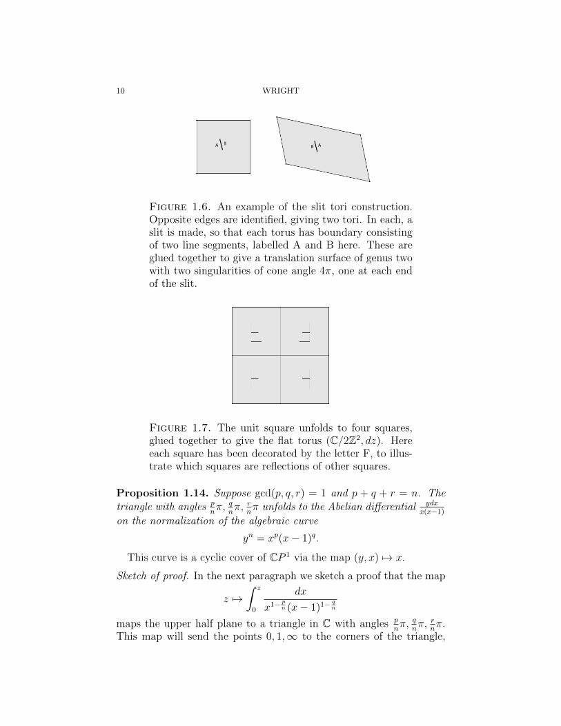
Figure 1.6. An example of the slit tori construction.Opposite edges are identified, giving two tori. In each, aslit is made, so that each torus has boundary consistingof two line segments, labelled A and B here. These areglued together to give a translation surface of genus twowith two singularities of cone angle 4π, one at each endof the slit.
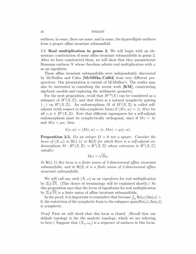
Figure 1.7. The unit square unfolds to four squares,glued together to give the flat torus (C/2Z2, dz). Hereeach square has been decorated by the letter F, to illus-trate which squares are reflections of other squares.
Proposition 1.14. Suppose gcd(p, q, r) = 1 and p + q + r = n. Thetriangle with angles p
nπ, q
nπ, r
nπ unfolds to the Abelian differential ydx
x(x−1)on the normalization of the algebraic curve
yn = xp(x− 1)q.
This curve is a cyclic cover of CP 1 via the map (y, x) 7→ x.
Sketch of proof. In the next paragraph we sketch a proof that the map
z 7→∫ z
0
dx
x1−pn (x− 1)1−
qn
maps the upper half plane to a triangle in C with angles pnπ, q
nπ, r
nπ.
This map will send the points 0, 1,∞ to the corners of the triangle,

FIVE LECTURES ON TRANSLATION SURFACES 11
Figure 1.8. Unfolding the right angled triangle withsmallest angle π/8 gives the regular octagon with oppo-site sides identified.
and the segments (−∞, 0), (0, 1) and (1,∞) to the edges, and will bea biholomorphism on the interior of the triangle. (The exact image ofthis map depends on the choice of n-th roots in the integral, which canbe made consistently over the upper half plane but not over the entireRiemann sphere.) These explicit uniformization maps are examples ofSchwarz-Christoffel mappings, a classical topic in complex analysis.
The argument of the integrand is constant along the real segments(−∞, 0), (0, 1) and (1,∞), and so each of these segments maps to astraight line in C. For z near zero, the integral is a nonzero holomorphicfunction times z
pn , and so the sector of the upper half plane at 0 maps to
an angle of pnπ. Similarly the sector of the upper half plane at 1 maps to
an angle of qnπ. Thus these three segments map to the desired triangle.
It can be verified that the upper half plane maps biholomorphically tothe interior of this triangle; for more details see [DT02], part of whichis available online here.
The algebraic curve in question consists of n lifts of the upper halfplane, and n lifts of the lower half plane, glued along lifts of (−∞, 0), (0, 1)and (1,∞). The above computation and the Schwarz reflection prin-ciple can be used to show that each lift of the upper half plane is flatisometric to a triangle with the desired angles, keeping in mind thatthe flat coordinate at nonsingular points is the integral of the Abeliandifferential. �
1.3. Moduli spaces. Consider the problem of deforming the regularoctagon. We may specify four of the edges as vectors in C, and thusguess (correctly!) that the moduli space is locally C4.

12 WRIGHT
Figure 1.9. An octagon with opposite edges parallelmay be specified by four complex numbers v1, v2, v3, v4 ∈C. (Not all choices give a valid octagon without selfcrossings, but there is an open set of valid choices.)
An Abelian differential in genus two can have either a double zero,or two zeros of order one. The octagon has a double zero, and defor-mations as above will always have a double zero. Figures 1.5 and 1.6illustrate genus two translation surfaces with two zeros of order one.
The collection of all Abelian differentials of genus g is of course avector bundle over the moduli space of Riemann surfaces. However,this space is stratified according to the number and multiplicity of thezeros of the Abelian differentials.
Let g > 1 and let κ denote a partition of 2g − 2, i.e. a nonin-creasing list of positive integers whose sum is 2g − 2. So if g =2, the partitions are (2) and (1, 1), and if g = 3 the partitions are(4), (3, 1), (2, 2), (2, 1, 1), (1, 1, 1, 1).
Define the stratum H(κ) as the collection of genus g translationssurfaces (X,ω), where the multiplicity of the zeros of ω are given byκ. So H(2) denotes the collection of genus two translation surfaceswith a double zero, and H(1, 1) denotes the collection of all genus twotranslation surfaces with two simple zeros.
Proposition 1.15. Each stratum H(κ) is a complex orbifold of dimen-sion n = 2g+ s− 1, where s = |κ| denotes the number of distinct zerosof Abelian differentials in the stratum. Away from orbifold points (oron an appropriate cover without orbifold points) each stratum has anatlas of charts to Cn with transition functions in GL(n,Z).
Thus each stratum looks locally like Cn, and has a natural affinestructure.
Sketch of formal proof. Let S be fixed topological surface of genus g,with a set Σ of s distinct marked points. Let us begin with the spaceH(κ) of translations surfaces (X,ω) equipped with an equivalence class

FIVE LECTURES ON TRANSLATION SURFACES 13
of homeomorphisms f : S → X that send the marked points to thezeros of ω. The equivalence relation is isotopy rel marked points.
We will see that the map from H(κ) to H(κ) that forgets f is aninfinite degree branched covering.
Fix a basis for the relative homology group H1(S,Σ,Z). If Σ ={p1, . . . , pn}, this is typically done by picking a (symplectic) basis
γ1, . . . , γ2g
for absolute homology H1(S,Z), and then picking a curve γ2g+i frompi to pn for each i = 1, . . . , n− 1. The map
H(κ)→ Cn, (X,ω, [f ]) 7→(∫
f∗γi
ω
)2g+s−1
i=1
is locally one-to-one and is onto an open subset of Cn. The easiest wayto see this is via flat geometry: These integrals determine the integralsof every relative homology class, and in particular the complex lengthsof the edges in any polygon decomposition for (X,ω). The edges inthis polygon decomposition of course determine (X,ω).
The mapping class group of S (with s distinct unlabeled markedpoints) acts on H(κ) by precomposition of the marking. The inducedaction on these Cn coordinates is via GL(n,Z) (change of basis forrelative homology). The quotient is H(κ). �
In this course we will ignore orbifold issues, and just pretend strataare complex manifolds rather than complex orbifolds (or stacks). Givena translation surface (X,ω), and a basis γi of the relative homologygroup H1(X,Σ,Z), we will refer to(∫
γi
ω
)2g+s−1
i=1
∈ Cn
as period coordinates near (X,ω). Implicit in this is that the basiscan be canonically transported to nearby surfaces in H(κ), thus givinga map from a neighbourhood of (X,ω) to a neighbourhood in Cn.However, when X has automorphisms preserving ω, this is not thecase canonically. This is precisely the issue we are ignoring when wepretend that H(κ) is a manifold instead of an orbifold.
It is precisely the period coordinates that provide strata an atlas ofcharts to Cn with transition functions in GL(n,Z). The transition func-tions are change of basis matrices for relative homology H1(X,Σ,Z).
Compactness criterion. Let us remark that strata are never com-pact. Even the subset of unit area translation surface is never compact.Here we are referring to the analytic topology, which is the weakest

14 WRIGHT
topology for which period coordinates are continuous. This analytictopology will be the default topology in these notes.
Masur’s compactness criterion gives that a closed subset of the setof unit area surfaces in a stratum is compact if and only if there issome positive lower bound for the length of all saddle connections onall translation surfaces in the subset.
Let us also remark that the map (X,ω) 7→ X is not proper, evenwhen restricting to unit area surfaces. For example, it is possible tohave a sequence of translation surfaces (Xn, ωn) of area 1 in H(1, 1)converge to (X,ω) ∈ H(2) (so two zeros coalesce) in the bundle ofAbelian differentials over the moduli space of Riemann surfaces. How-ever, such a sequence (Xn, ωn) will diverge in H(1, 1): there will beshorter and shorter saddle connections joining the two zeros.
Every Abelian differential in genus two. We now give flat ge-ometry pictures of all Abelian differentials in genus 2. The discussionincludes only sketches of proofs.
Proposition 1.16. Every translation surface in H(2) can be obtainedby gluing a cylinder into a slit torus, as in figure 1.10. Every translationsurface in H(1, 1) is obtained from the slit torus construction, as infigure 1.11
Lemma 1.17. For any translation surface in genus 2, not every saddleconnection is fixed by the hyperelliptic involution ρ.
Proof. Triangulate the surface. If every saddle connection in this tri-angulation was fixed by the hyperelliptic involution, then each trianglewould be mapped to itself. However, no triangle has rotation by πsymmetry, so this is impossible. �
Sketch of proof of proposition. Now fix a translation surface in H(2),and a saddle connection c not fixed by ρ. Since ρ∗ acts on homology by−1, c and ρ(c) are homologous curves. Cutting c and ρ(c) decomposesthe surface into two subsurfaces with boundary, one of genus one andone of genus zero. The genus zero component is a cylinder and thegenus one part must be a slit torus.
Similarly for a translation surface inH(1, 1), consider a triangulation.This must contain at least one triangle with one vertex at one of thesingularities, and the other two vertices at the other singularity (i.e., forat least one of the triangles, not all corners are at the same singularity).At most one of the edges of this triangle is fixed by the hyperellipticinvolution, so the triangle must have at least one edge c that is notfixed by the hyperelliptic involution and goes between the two zeros.

FIVE LECTURES ON TRANSLATION SURFACES 15
Figure 1.10. Every translation surface in H(2) admitsa deposition into a cylinder and a slit torus, and hencecan be drawn as in this picture. Opposite sides are iden-tified.
Cutting along c and ρ(c) decomposes the surface into two tori. Inother words, every translation surface in H(1, 1) may be obtained fromthe slit torus construction.
Figure 1.11. Every translation surface in H(1, 1)comes from the slit torus construction, and thus can bedrawn as in this picture.
�
Philosophical conclusions. Polygon decompositions and flat geom-etry provide a fundamentally different way to think about Abelian dif-ferentials on complex algebraic curves. In this perspective an Abeliandifferential is extremely easy to write down (as a collection of polygons),and it is easy to visualize deformations of this Abelian differential (theedges of the polygons change). However, some things become moredifficult in this perspective. For example, given a plane algebraic curveit is often an easy exercise to write down a basis of Abelian differen-tials. However, given a translation surface given in terms of polygons,this is typically impossible to do. And it is typically a transcendentallydifficult problem to write down the equations for the algebraic curvegiven by some polygon decomposition.

16 WRIGHT
The study of translation surfaces and algebraic curves is enriched bythe transcendental connections between the two perspectives.
Exercises.
(1) Prove that square-tiled surfaces are dense in every stratum. (Thedefinition of square-tiled surface has to be relaxed for this exercise.Instead of just covers of the unit area (C/Z2, dz), covers of scalingsof this (C/(cZ2), dz) should also be allowed.)
(2) Prove that a translation surface covers a torus iff the absolute pe-riods span a rank 2 Q-module. The absolute periods of (X,ω) are{∫γω : γ ∈ H1(X,Z)}.
(3) Using the second definition of translation surface, prove that everytranslation surface of genus at least two has a saddle connection.(This is a step in showing that every such surface can be triangu-lated. Hint: Think about embedding larger and larger balls, untilthe boundary of the ball eventually touches itself.)
(4) Prove that, for any translation surface (X,ω) and for any T > 0,there are finitely many saddle connections on (X,ω) of length atmost T .
(5) Can a translation surface in H(3, 1) be hyperelliptic?(6) Draw a flat picture of a translation surface in the stratumH(2, 1, 1, 1, 1),
by starting with a translation surface inH(2) and gluing on slit tori.What is the genus?
(7) Prove Proposition 1.14 without using Schwarz-Christoffel mappings.(Hint: Straight from the definition, you should be able to show thatthe Riemann surface has an automorphism. In the case of trian-gles, prove the quotient is CP 1, and the quotient map is branchedover 3 points.)
(8) Prove that H(2) and H(1, 1) are both path connected. Bonus:Show that H(4) is not (there is one connected component thatconsists entirely of hyperelliptic surfaces, and another that doesnot).
(9) Research problem: are connected components of strata K(π, 1)’s?(It is conjectured by Kontsevich that they are, however, I am notaware of any reason why this should be so. The problem is openfor most strata starting in genus 4. See [LM14] for a resolution ingenus 3.)
(10) Research problem: Say something about the birational geometryof strata.

FIVE LECTURES ON TRANSLATION SURFACES 17
2. Affine invariant submanifolds
2.1. Definitions and first examples. Recall that (ignoring orbifoldissues), each stratum has an atlas of charts (called period coordinates)to Cn with transition functions in GL(n,Z). As a review, lets reviewperiod coordinates from a slightly different point of view. Fix a stra-tum, and a translation surface (X,ω) in the stratum. As always, letΣ ⊂ X be the zeros of ω.
There is a linear injection H1,0(X) → H1(X,Σ,C)∗ = H1(X,Σ,C).Given ω ∈ H1,0(X), the linear functional it determines in H1(X,Σ,C)∗
is simply integration of ω over relative homology classes. Then, givena basis γ1, . . . , γn of H1(X,Σ,Z), we get an isomorphism
H1(X,Σ,C)→ Cn, φ 7→ (φ(γi))ni=1 .
The period coordinates of the previous section are just the composi-tion of the map sending (X,ω) to ω considered as a relative cohomol-ogy class, followed by this isomorphism to Cn. About half the timeit is helpful to forget this coordinatization, and just consider periodcoordinates as a map to H1(X,Σ,C) sending (X,ω) to the relativecohomology class of ω.
In the next definition we fix a stratum H = H(κ), where κ is apartition of 2g − 2 and g is the genus.
Definition 2.1. An affine invariant submanifold is the image of aproper immersion f of an open connected manifold M to a stratumH, such that each point p of M has a neighbourhood U such that ina neighbourhood of f(p), f(U) is determined by linear equations inperiod coordinates with coefficients in R and constant term 0.
The difference between immersion and embedding is a minor tech-nical detail, so for notational simplicity we will typically consider anaffine invariant submanifold M to be a subset of a stratum. The def-inition says that locally in period coordinates, M is a linear subspaceof Cn. The requirement that the linear equations have coefficients inR is equivalent to requiring that the linear subspace of Cn is the com-plexification of a real subspace of Rn (or, in coordinate free terms, ofH1(X,Σ,R)).
The word “affine” does not refer to affine varieties; it refers to thelinear structure on Cn. (Perhaps “linear” would be a better term than“affine”, but this is the terminology in use.)
In these notes, when we refer to the dimension of complex manifoldsor vector spaces, we will mean their complex dimension. So, for exam-ple, when we speak of 2-dimensional affine invariant submanifolds, we

18 WRIGHT
Figure 2.1. Period coordinates (v1, v2, v3, v4, v5) ∈ C5
have been indicated on two surfaces in H(1, 1) (upperand lower left) that are degree four translation coversof tori (upper and lower right). The linear equationsindicated locally cut out the locus of surfaces in H(1, 1)that are degree four translation covers of tori branchedover 1 point.
will be referring to objects of complex dimension 2 and real dimension4.
Note that affine invariant submanifolds must have dimension at least2. This is because if (X,ω) is a point on an affine invariant submanifold,then the linear subspace must contain the real and imaginary parts theperiod coordinates, and these cannot be collinear. That they cannotbe collinear follows from the fact that Re(ω) and Im(ω) cannot becollinear real cohomology classes, because∫
X
Re(ω) Im(ω)
gives the area of the translation surface. (Locally ω = dz = dx + idy,so Re(ω) Im(ω) = dxdy.)
Example 2.2. LetM be a connected component of the space of degreed translation covers of a genus one translation surface, which is allowed

FIVE LECTURES ON TRANSLATION SURFACES 19
to vary, branched over k distinct points. ThenM is an affine invariantsubmanifold of whichever stratum it lies in.
Indeed, M is a (k + 1)-dimensional immersed manifold: the modulispace of genus one translation surfaces is 2-dimensional, and after onebranched point is fixed at 0, the other k − 1 are allowed to vary onthe torus. So it suffices to see that locally in period coordinates, M iscontained in an (k + 1)-dimensional linear subspace.
Let (X,ω) ∈ M, and say f : (X,ω) → (X ′, ω′) is the translationcovering, branched over k points. Let Σ ⊂ X be the set of zeros of ω,and Σ′ ⊂ X ′ be the set of branch points of f , so f(Σ) = Σ′.
Let γ ∈ ker(f∗) ⊂ H1(X,Σ,Z), and note that∫γ
ω =
∫γ
f ∗(ω′)
=
∫f∗γ
ω′ = 0.
Thus since ker(f∗) has dimension dimCH1(X,Σ,C)−dimCH1(X′,Σ′,C),
we see that locallyM lies in an dimCH1(X′,Σ′,C) = (k+1)-dimensional
linear subspace in period coordinates, as desired.To rephrase the discussion, the relative cohomology class of ω lies in
f ∗(H1(X ′,Σ′,C)).
Example 2.3. Fix a stratum H and numbers k and d, and let M bea connected component of the space of all degree d translation coversof surfaces in H branched over k ≥ 0 distinct points. Then similarlyM is an affine invariant submanifold.
Similarly, if M is an affine invariant submanifold, and M′ is a con-nected component of the space of all degree d translation covers ofsurfaces in M branched over k ≥ 0 distinct points, then M′ is also anaffine invariant submanifold.
Example 2.4. Fix a stratum H and a number k, and let Q be aconnected component of the locus of (X,ω) ∈ H where X admits aninvolution ι with ι∗(ω) = −ω and k fixed points. Then Q is an affineinvariant submanifold of H (although it may be empty). It is locallydefined by the equations ∫
ι∗γ
ω +
∫γ
ω = 0,
for γ ∈ H1(X,Σ,Z).A special case of this example is when ι is the hyperelliptic involution.
In some strata, there is a whole connected component of hyperelliptic
20 WRIGHT
surfaces; in some, there are none; and in some, the hyperelliptic surfacesform a proper affine invariant submanifold.
2.2. Real multiplication in genus 2. We will begin with an ele-mentary construction of some affine invariant submanifolds in genus 2.After we have constructed them, we will show that they parameterizeRiemann surfaces X whose Jacobian admits real multiplication with ωas an eigenform.
These affine invariant submanifolds were independently discoveredby McMullen and Calta [McM03a, Cal04] from very different per-spectives. Our presentation is variant of McMullen’s. The reader mayalso be interested in consulting the recent work [KM], constructingalgebraic models and exploring the arithmetic geometry.
For the next proposition, recall that H1,0(X) can be considered as asubspace of H1(X,C), and that there is a natural symplectic pairing〈·, ·〉 on H1(X,Z). An endomorphism M of H1(X,Z) is called self-adjoint (with respect to this symplectic form) if 〈Mv,w〉 = 〈v,Mw〉 forall v, w ∈ H1(X,Z). Note that different eigenspaces for a self-adjointendomorphism must be symplectically orthogonal, since if Mv = λvand Mw = µw, then
λ〈v, w〉 = 〈Mv,w〉 = 〈v,Mw〉 = µ〈v, w〉.
Proposition 2.5. Fix an integer D > 0 not a square. Consider thelocus of (X,ω) in H(1, 1) or H(2) for which there is a self-adjoint en-domorphism M : H1(X,Z) → H1(X,Z) whose extension to H1(X,C)satisfies
Mω =√Dω.
In H(1, 1) this locus is a finite union of 3-dimensional affine invariantsubmanifolds, and in H(2) it is a finite union of 2-dimensional affineinvariant submanifolds.
We will call any such (X,ω) as an eigenform for real multiplication
by Z[√D]. (This choice of terminology will be explained shortly.) So
this proposition says that the locus of eigenforms for real multiplicationby Z[
√D] is a finite union of affine invariant submanifolds.
In the proof, it is important to remember that because∫X
Re(ω) Im(ω) >0, the restriction of the symplectic form to the subspace span(Re(ω), Im(ω))is symplectic.
Proof. First we will check that this locus is closed. (Recall that ourdefault topology is the the analytic topology, which we are referringto here.) Suppose that (Xn, ωn) is a sequence of surfaces in this locus,

FIVE LECTURES ON TRANSLATION SURFACES 21
converging to (X,ω). We will first show that necessarily (X,ω) is inthe locus, and hence the locus is closed.
Let Mn denote the endomorphism for (Xn, ωn). This endomorphism
Mn has two√D-eigenvectors, Re(ωn) and Im(ωn). Since Mn is an
integer matrix, its −√D-eigenspace is the Galois conjugate of its
√D-
eigenspace, and hence must also be 2-dimensional. Since Mn is self-adjoint, the
√D and −
√D-eigenspaces are symplectically orthogonal.
In particular, the −√D-eigenspace is the symplectic perp of the
√D-
eigenspace.Note that ωn converges to ω as cohomology classes. (The topology
on strata is the topology on period coordinates, and period coordi-nates exactly determine the relative cohomology class of ω.) Hence Mn
converges to an endomorphism M of H1(X,Z), which acts by√D on
span(Re(ω), Im(ω)) and by −√D on the symplectic perp. Thus (X,ω)
is in the locus also, and we have shown the locus is closed.We must now show linearity. For this, it is important to note that
above, since End(H1(X,Z)) is a discrete set, we see that Mn is in facteventually constant. So any (X ′, ω′) in the locus close to (X,ω) hasthe same endomorphism.
Suppose (X,ω) is in the locus, with endomorphism M . Consider the
set of (X ′, ω′) sufficiently close to (X,ω) for which Mω′ =√Dω. Since
this equation is linear, we see that locally the locus is linear.In other words, ω′ must lie in the 2-dimensional
√D-eigenspace in
H1(X,C). In the 4-dimensionalH(2) the set of such ω′ is 2-dimensional,however in the 5-dimensionalH(1, 1), this set is 3-dimensional. (Periodcoordinates for H(2) may be considered as a map to H1(X,C), and forH(1, 1) they may be considered as a map to H1(X,Σ,C). There is anatural map from H1(X,Σ,C) to H1(X,C), and we are requiring thatthe image of ω lies in a codimension 2 subspace there.) �
We can be more explicit about the linear equations that define thelocus in period coordinates. Indeed, suppose that γ1, γ2 ∈ H1(X,Z) aresuch that γ1, γ2,M
∗γ1,M∗γ2 are a basis, where M∗ denotes the dual
linear endomorphism of H1(X,Z). Then the linear equations are∫M∗γi
ω =√D
∫γi
ω, for i = 1, 2.
Examples of eigenforms. Before we explain the terminology, wewill show that eigenforms actually exist in H(2), by giving explicitexamples. That is, we will show that the loci above are nonempty.(We won’t prove it, but we will give enough examples to account forall connected components for all eigenform loci in H(2).) A similar

22 WRIGHT
argument could show that eigenforms exist in H(1, 1) (but in H(1, 1)there is a softer argument as well, using the fact that most PPAV areJacobians in genus 2).
Proposition 2.6. The surfaces indicated in figure 2.2 are eigenformsfor real multiplication by
√mD for some integer m > 0.
Figure 2.2. Opposite sides are identified, and all edgesare vertical or horizontal. The numbers indicate signedreal length in the direction indicated, and the parametersx, z are rational.
Lemma 2.7. For the translation surface (X,ω) in figure 2.2,
span(Re(ω), Im(ω))
is symplectically orthogonal to the Galois conjugate subspace of H1(X,ω).
Proof. Since the periods of ω are in Q[√D, i], we can define a cohomol-
ogy class ω′ in H1(X,Q[√D, i]) that is Galois conjugate to ω. Note
that ω′ is not expected to be represented by a holomorphic 1-form. Itcan be described more concretely via the isomorphism
H1(X,Q[√D, i]) = Hom(H1(X,Z),Q[
√D, i]).
From this point of view, ω′ is the composition of ω with the field en-domorphism of Q[
√D, i] that fixes i and sends
√D to −
√D.
In figure 2.3, note that α1, β1, α2, β2 − β1 is symplectic basis of ho-mology. So, if φ, ψ ∈ H1(X,R) = Hom(H1(X,R),R), we can computetheir symplectic pairing as
〈φ, ψ〉 = φ(α1)ψ(β1)− φ(β1)ψ(α1) +
φ(α2)ψ(β2 − β1)− φ(β2 − β1)ψ(α2).

FIVE LECTURES ON TRANSLATION SURFACES 23
Figure 2.3. A basis of homology is indicated.
Suppose that we set Aj = 1i
∫αjω and Bj =
∫βjω. We are assuming
that B1 = 1 = A2. Then we may compute
〈Im(ω),Re(ω′)〉 = A1B′1 + A2(B
′2 −B′1)
= A1 −B′2 − 1.
If A1 = x+ z√D and B2 = y +w
√D, this quantity is zero if and only
if x− y = 1 and w = −z.Both 〈Re(ω),Re(ω′)〉 and 〈Im(ω), Im(ω′)〉 are easily seen to be auto-
matically zero, and 〈Re(ω), Im(ω′)〉 is the Galois conjugate of−〈Im(ω),Re(ω′)〉.Hence these conditions x − y = 1 and w = −z are equivalent to theorthogonally of span(Re(ω), Im(ω)) and span(Re(ω′), Im(ω′)). �
Proof of proposition. We defineM0 to be the endomorphism ofH1(X,R)
that acts by√D on span(Re(ω), Im(ω)) and by −
√D on the Galois
conjugate subspace span(Re(ω′), Im(ω′)). This matrix is rational, andit is self-adjoint if and only if span(Re(ω), Im(ω)) and span(Re(ω′), Im(ω′))are symplectically orthogonal.
SinceM0 is a rational matrix, for somem > 0 we get thatM = m2M0
is integral. �
Connection to real multiplication. Recall that the complex vectorspace H1,0(X) is canonically isomorphic as a real vector to H1(X,R),via the map ω 7→ Re(ω). The natural symplectic form on H1(X,R)pulls back to the pairing
〈ω1, ω2〉 =1
2Re
(∫ω1ω2
)on H1,0(X). This symplectic form on H1,0(X) is compatible withthe complex structure on H1,0(X), in that 〈iω1, iω2〉 = 〈ω1, ω2〉 and−〈ω, iω〉 > 0 for all ω 6= 0.

24 WRIGHT
We will let H1,0(X)∗ denote the dual of the complex vector spaceH1,0(X). As a real vector space, H1,0(X)∗ is canonically isomorphic toH1(X,R), via the usual integration pairing between homology classesand Abelian differentials. The space H1,0(X)∗ inherits a dual compat-ible symplectic pairing, which we will also denote 〈·, ·〉.
Definition 2.8. The Jacobian Jac(X) of a Riemann surface X is thecomplex torus H1,0(X)∗/H1(X,Z), together with the data of the sym-plectic pairing 〈·, ·〉 on its tangent space to the zero. (This tangent spaceis H1,0(X)∗.) An endomorphism of Jac(X) is an endomorphism of thecomplex torus that induces a self-adjoint endomorphism of H1,0(X)∗.
Thus, endomorphisms of Jac(X) can be thought of either as self-adjoint complex linear endomorphisms ofH1,0(X)∗ that preservesH1(X,Z),or as self-adjoint linear endomorphisms of H1(X,Z) whose real linearextension to H1,0(X)∗ happens to be complex linear. From our pointof view, the second perspective is more enlightening, and the require-ment of complex linearity is the deepest part of the definition. Thisis because the complex structure on H1,0(X)∗ is determined by howH1,0(X) sits in H1(X,C), i.e., the Hodge decomposition. The Hodgedecomposition varies as the complex structure on X varies, in a some-what mysterious way. The complex linearity restriction is the only partof the data of an endomorphism of Jac(X) that depends on the com-plex structure on X (the rest could be defined for a topological surfaceinstead of a Riemann surface).
Recall that a totally real field is a finite field extension of Q, all ofwhose field embeddings into C have image in R. Every real quadraticfield is totally real, but there are cubic real fields that are not totallyreal, for example Q[2
13 ]. An order in a number field is just a finite
index subring of the ring of integers.
Definition 2.9. A genus g surface X is said to have real multiplicationby an order O in a totally real number field if O acts on Jac(X) byendomorphisms and the totally real field has degree g. An Abeliandifferential ω ∈ H1,0(X) is said to be an eigenform for this action if itis an eigenvector for the induced action of O on the cotangent space ofJac(X) at 0. (This cotangent space is H1,0(X).)
Genus two is special for real multiplication because of the following.
Lemma 2.10. Fix a compatible symplectic structure on C2, and let M :C2 → C2 be a self-adjoint real linear endomorphism. If M preserves acomplex line L ∈ C2, then M is complex linear.

FIVE LECTURES ON TRANSLATION SURFACES 25
Proof. First note, that the only self-adjoint real linear endomorphismsof R2 are scalars times identity. (This can be verified in coordinates,for 2 by 2 matrix and the standard symplectic form on R2.)
Since the symplectic form is compatible, L⊥ is a complex line. Mleaves invariant the two complex lines L and L⊥, and acts as a scalaron each, so it must be complex linear. �
It follows from this that
Theorem 2.11 (McMullen). The eigenform loci in H(2) and H(1, 1)as defined above in fact parameterize (X,ω) where Jac(X) admits real
multiplication by Z[√D] with ω as an eigenform.
Proof. From the definition of the eigenform loci we get a self-adjointaction of Z[
√D] on H1(X,Z), where
√D acts by M . This gives a
dual action on H1(X,R), which preserves H1(X,Z). It suffices to showthat this action is complex linear. This follows from the lemma, andthe observation that the complex line consisting of the annihilator ofspan(Re(ω), Im(ω)) is preserved by the action. �
Remark 2.12. It is important to note the proof of Proposition 2.5doesn’t work in higher genus. This is because the Mn are not guar-anteed to converge (they might diverge). (Here we fix a generator foran order in a totally real number field, and Mn is the action of thisgenerator.)
Given that the Mn are automatically complex linear in genus 2, itis natural to impose this condition in higher genus, and try to seeif loci of eigenforms as defined in definition 2.9 give affine invariantsubmanifolds. With the complex linearity, it turns out the Mn mustconverge, which at least lets you show the locus is closed.
However, even with complex linearity the end result isn’t true, be-cause even if M is complex linear at (X,ω), there is no reason forthis to be true at (X ′, ω′). So in higher genera eigenforms are locallycontained in nice linear spaces, but the real multiplication can vanishas you move from an eigenform (X,ω) to a nearby translation surface(X ′, ω′) whose periods satisfy the same linear equations.
2.3. Torsion, RM, and algebraicity. There is however a still a verystrong connection between endomorphisms of Jacobians and affine in-variant submanifolds in higher genus, as discovered by Moller in thecase that the affine invariant submanifold has complex dimension 2.
Definition 2.13. Given (X,ω), let V ⊂ H1(X,Q) be the smallestsubspace such that V ⊗C contains ω, and such that V ⊗C = V 1,0⊕V 0,1,

26 WRIGHT
whereV 1,0 = (V ⊗ C) ∩H1,0 and V 0,1 = V 1,0.
Set V ∗Z = {φ ∈ V ∗ : φ(V ∩H1(X,Z)) ⊂ Z}. Define
Jac(X,ω) = (V 1,0)∗/V ∗Z ,
together with the data of the symplectic form on V ∗. (This objectJac(X,ω) does not have a standard name.)
V obtains a symplectic form by restriction from H1(X,Q). Therestriction is automatically symplectic (i.e., nondegenerate) because ofthe condition V ⊗ C = V 1,0 ⊕ V 0,1. The symplectic form on V ∗ is thedual symplectic form.
Jac(X,ω) is a factor of Jac(X) up to isogeny, and it the “smallestfactor containing ω”.
Definition 2.14. Let p, q be two points of (X,ω). We say that p− qis torsion in Jac(X,ω) if, for any relative homology class γp,q of acurve from p to q, there is a γ ∈ H1(X,Q) such that for all ω′ ∈ V 1,0
(including the most important one ω′ = ω),∫γp,q
ω′ =
∫γ
ω′.
If Jac(X,ω) = Jac(X), this is equivalent to p−q being torsion in thegroup Jac(X). For every affine invariant submanifold M of complexdimension two, there is a natural algebraic extension of Q called thetrace field, which will be defined in the final lecture. The definition ofreal multiplication on Jac(X,ω) is exactly analogous to that for Jac(X),except the degree of the field is required to be equal to the complexdimension of Jac(X,ω), which is sometimes less than g, and the orderis required to act on Jac(X,ω) (instead of Jac(X)).
Theorem 2.15 (Moller [Mol06b,Mol06a]). For every affine invari-ant submanifold M of complex dimension two, and every (X,ω) ∈M,Jac(X,ω) has real multiplication by the trace field with ω as an eigen-form, and furthermore if p and q are zeros of ω, then p− q is torsionin Jac(X,ω).
This result is actually two deep theorems, and their importance forthe field is very great. One might expect that, given that an affineinvariant submanifold is defined in terms of (X,ω), the other holo-morphic 1-forms on X would not be special, but this result says thatthey are (since the definition of torsion involves all or many ω′, andreal multiplication produces other eigenforms for the Galois conjugateeigenvalues).

FIVE LECTURES ON TRANSLATION SURFACES 27
The converse of Moller’s result is true, and is much easier than theresult itself.
Proposition 2.16 (Wright). Let M be a 2-dimensional submanifoldof a stratum (not assumed to be linear), and suppose that for every(X,ω) ∈M, Jac(X,ω) has real multiplication by the trace field with ωas an eigenform, and furthermore if p and q are zeros of ω, then p− qis torsion in Jac(X,ω). Then M is an affine invariant submanifold.
Proof. We must show thatM is locally linear. For notational simplic-ity, we will assume Jac(X,ω) = Jac(X).
There are only countably many totally real number fields of degree g,and only countably many actions of each on H1(X,Q). Since the locusof eigenforms for each is closed, we may assume that the totally realnumber field is constant, and the action on H1(X,Q) is locally con-stant. (Again, this is a simple connectivity argument: The connectedspace M is covered by disjoint closed sets, so there can only be one.)
Similarly, we can assume that for each pair of zeros p, q of ω, therational homology class γ in definition 2.14 is locally constant.
We will show that the span of Re(ω) and Im(ω) does not change inH1(X,Σ,C). This span gives the linear subspace that locally definesM.
The real multiplication condition gives that the image of this spanis locally constant in absolute homology (it is an eigenspace), and thetorsion condition gives that each relative period
∫γp,q
ω is equal to an
absolute period∫γω, and hence the relative periods are determined by
absolute periods.That concludes the proof, but in closing we will write down the linear
equations explicitly at (X,ω) ∈M. Say the number field is k and hasQ-basis r1, . . . , rg. Pick two absolute homology classes γ1, γ2 so thatthe
ρ(ri)γj, i = 1, . . . , g, j = 1, 2,
are a basis for H1(X,Q). Say the zeros of ω are p1, . . . , ps, and let αibe a relative cycle from pi to ps, for i = 1, . . . , s − 1. For each i, letα′i ∈ H1(X,Q) be given from αi by definition 2.14. Then the equationsare ∫
ρ(ri)γj
ω = ri
∫γj
ω, i = 1, . . . , g, j = 1, 2,
and ∫αi
ω =
∫α′i
ω, i = 1, . . . , s− 1.
�

28 WRIGHT
Recently, Simion Filip has generalized Moller’s result to affine invari-ant submanifolds of any dimension. As in the previous proposition,this gives enough algebro-geometric conditions to characterize affineinvariant submanifolds, and so Filip is able to conclude the following[Filb,Fila].
Theorem 2.17 (Filip). All affine invariant submanifolds are quasi-projective varieties.
Filip’s proof crucially uses dynamics, and no other proof is known.
Exercises.
(1) Prove that the regular 8-gon is contained in a 2-dimensional affineinvariant submanifold. Write down the linear equations definingthis in period coordinates.
(2) Consider all degree d translation covers of a torus, branched overzero and k other distinct points whose sum is zero in the torus.Show that any connected component of this space is an affine in-variant submanifold.
(3) Verify the torsion condition for covers of tori branched at one point.(4) Say that a translation surface is primitive if it does not cover a
translation surface of lower genus, or if it is genus 1. Show thatevery translation surface covers a primitive surface, which is uniqueif it is not a torus. (This is a nontrivial theorem of Moller, but youmight rediscover the proof if you think about natural maps fromX to Abelian varieties finitely covered by Jac(X,ω).)
(5) Prove that if a 2-dimensional affine invariant submanifold containsa single cover of a torus, then every translation surface in the sub-manifold is a cover.
(6) Easier research problem: Read about the Veech-Ward-Bouw-Mollercurves in [Wri13], and then give a new proof that they are 2-dimensional affine invariant submanifolds using Proposition 2.16.
(7) Research problem: Determine which unfoldings of triangles are con-tained in 2-dimensional affine invariant submanifolds. (Quite a bitis known, but even more is unknown. There is a conjectural an-swer: in short, not many.) An answer was announced for acuterational triangles in [KS00, Puc01], but I have found a gap inthe proof caused by a typo at the interface of the two papers. Ihave adapted the proof of Theorem 7.5 in [McM03a] to show thata great many triangles are not contained in 2-dimensional affineinvariant submanifolds, but I can’t handle all triangles.
(8) Research problem: Find an example of an affine invariant subman-ifold that is not embedded (but only immersed). I don’t think

FIVE LECTURES ON TRANSLATION SURFACES 29
anyone has tried to do this yet, and examples may be constructibleusing covering constructions (the locus of surfaces that translationcovered something lower genus in two different ways might lead toself crossings of the immersed manifold).
(9) Research problem: Find a proof that affine invariant submanifoldsare varieties that does not use any dynamics. Currently the proofuses dynamics. Even just in the smallest case of 2-dimensionalaffine invariant submanifolds a new proof would be very interesting.
(10) Research problem: Determine if affine invariant submanifolds arevarieties when the definition is relaxed to allow the linear equationsto have complex coefficients.
(11) Research problem: Prove that, for g sufficiently large (or for anyparticular g > 2), in the stratum of genus g surfaces with 2g − 2distinct zeros of order 1 there are no 2-dimensional affine invariantsubmanifolds where Jac(X,ω) = Jac(X). (This last condition iscalled algebraic primitivity, and guarantees in particular that (X,ω)does not cover a lower genus surface.) I am not sure this is true,but it seems very likely to be true. In genus two there is only onesuch object (proven by McMullen [McM06b] using the torsioncondition of Moller), and all higher general there are none known.
3. The action of GL+(2,R)
This lecture will begin to set the stage for the following driving themein the study of translation surfaces.
The behavior of certain dynamical systems is fundamentally linked tothe structure of affine invariant submanifolds.
The dynamical systems involved are the action of GL+(2,R) on eachstratum, which is the topic of this lecture, and the straight line flow oneach individual translation surface, which is the topic of the next lec-ture. It is very important to note that the connections go in both direc-tions: Dynamical information often powers structural results on affineinvariant submanifolds, and in the opposite direction results about thestructure of linear manifolds are crucial in the study of the dynamicalproblems.
3.1. Definitions and basic properties. In this section, it is mosthelpful to think of a translation surface using the third definition (poly-gons). Let GL+(2,R) be the group of two by two matrices with positivedeterminant.
There is an action of GL+(2,R) on each stratum H induced fromthe linear action of GL+(2,R) on R2. If g ∈ GL+(2,R), and (X,ω) is

30 WRIGHT
a translation surface given as a collection of polygons, then g(X,ω) isthe translation surface given by the collection of polygons obtained byacting linearly by g on the polygons defining (X,ω).
Naively, one might thing that g(X,ω) is always very different from(X,ω) when g is a large matrix, because g distorts any polygon a largeamount. But because of the cut and paste equivalence, this is not thecase. For example,
Proposition 3.1. The stabilizer of the (C/Z2, dz) is GL+(2,Z) =SL(2,Z). The stabilizer of any square-tiled surface is a finite indexsubgroup of GL+(2,Z).
Proof. Note that g(C/Z2, dz) = (C/g(Z2), dz). This gives that the sta-bilizer of (C/Z2, dz) is exactly the matrices g ∈ GL+(2,R) preservingZ2 ⊂ R2. Hence the stabilizer of (C/Z2, dz) is SL(2,Z).
In general, the stabilizer preserves the periods of a surface. For asquare-tiled surface, the periods are Z2, so for any square-tiled surfacethe stabilizer is a subgroup of SL(2,Z).
Now, suppose (X,ω) is a square-tiled surface. For any g ∈ SL(2,Z),g(X,ω) is a square-tiled surface with the same number of squares.Hence, the stabilizer of (X,ω) is finite index in SL(2,Z). �
More basic properties are
Proposition 3.2. The SL(2,R)-orbit of every translation surface isunbounded. The stabilizer of every translation surface is discrete butnever cocompact in SL(2,R).
Proof. If g ∈ GL+(2,R) is close enough to the identity, then g(X,ω)and (X,ω) are in the same coordinate chart. The coordinates ofg(X,ω) are obtained from those of (X,ω) by acting linearly on C = R2.This shows that for g sufficiently small enough and not the identity,g(X,ω) 6= (X,ω), because they have different coordinates. Hence thestabilizer is discrete.
Set
rθ =
(cos(θ) − sin(θ)sin(θ) cos(θ)
)and gt =
(et 00 e−t
).
For every (X,ω), there is some θ such that rθ(X,ω) has a verticalsaddle connection. (Pick any saddle connection, and rotate so that it

FIVE LECTURES ON TRANSLATION SURFACES 31
becomes vertical.) On gtrθ(X,ω) this saddle connection is e−t timesas long, so as t → ∞, we see that gtrθ(X,ω) has shorter and shortersaddle connections and hence diverges to infinity in the stratum.
Let Γ be the stabilizer of (X,ω), and suppose (X,ω) lies in thestratum H. Consider the natural orbit map
SL(2,R)/Γ→ H, [g] 7→ g(X,ω).
By definition, Γ is cocompact if SL(2,R)/Γ is compact. If SL(2,R)/Γwere compact, then its image under this map would be compact also.However, the image is just the SL(2,R)-orbit of (X,ω), which must beunbounded and hence cannot be compact. �
Definition 3.3. A cylinder on a translation surface is an isometricallyembedded copy of a Euclidean cylinder (R/cZ)×(0, h) whose boundaryis a union of saddle connections. The number c is the circumference,and the number h is the height of the cylinder. The ratio h/c is themodulus of the cylinder. The direction of the cylinder is the direction ofits boundary saddle connections (so directions are formally elements ofRP 1). A translation surface (X,ω) is called periodic in some direction(X,ω) is the union of the cylinders in that direction together with theirboundaries.
Figure 3.1. On the left octagon (with opposite sidesidentified), both the shaded part and its complement arehorizontal cylinders. On the right octagon, the shadedrectangle is not a cylinder according to our definition,because its boundary is not a union of saddle connec-tions. The effect of requiring the boundary to consist ofsaddle connections is equivalent to requiring the cylin-ders to be “maximal”, unlike this example on the right,whose height could be increased. The regular octagon ishorizontally periodic, since it is the union of two hori-zontal cylinders (and their boundaries).

32 WRIGHT
Proposition 3.4. A translation surface contains a matrix of the form(1 t0 1
)in its stabilizer if the surface is horizontally periodic, and all reciprocalsof moduli of horizontal cylinders are integer multiples of t.
Figure 3.2. Each individual cylinder is stabilized bya parabolic matrix. In this picture, opposite edges areidentified, except for the horizontal edges, which are theupper and lower boundary of the cylinder. The cylinderon the right can be cut along the dotted line and re-gluedto give the cylinder on the left.
Proof. The proof is essentially just Figure 3.2. Each horizontal cylinderof modulus m is stabilized by the matrix(
1 m−1
0 1
).
�
Note that both the previous and next proposition apply to any direc-tion (not just horizontal) by first rotating the surface. They are statedfor the horizontal direction only for notational simplicity.
Proposition 3.5. If (X,ω) is stabilized by the matrix(1 t0 1
),
then (X,ω) is horizontally periodic and the ratios of moduli of horizon-tal cylinders are all rational.
This requires a lemma, whose proof will be omitted but is very similarto proofs that will be covered in detail in the next lecture.
Lemma 3.6. Suppose (X,ω) is not horizontally periodic. Then thereare saddle connections γ such that
∫γω = x+iy with y arbitrarily small
and nonzero. (Generally the smaller y is, the more enormous x is.)

FIVE LECTURES ON TRANSLATION SURFACES 33
Proof of Proposition. First note that the
us =
(1 s0 1
)orbit of (X,ω) is a circle (since us+t(X,ω) = us(X,ω)); in particularit is compact and hence bounded. If there was a saddle connection ofcomplex length x + iy, then on us(X,ω) with s = −x/y this saddleconnection has length y. Since the us-orbit is bounded, there must bea lower bound on |y|, and so the lemma gives that (X,ω) is horizontallyperiodic.
We assume that ut fixes the surface, which means that ut appliedto a polygon decomposition gives a polygon decomposition that canbe cut up and re-glued to give the original. As the cylinders are cutand re-glued they might be permuted. But some finite power of utmust fix the surface in a way that the cylinders and horizontal saddleconnections are not permuted in this way. This power of ut mustindividually stabilize each cylinder and horizontal saddle connection.The result then follows by observing that the stabilizer of a cylinder ofmodulus m is exactly the group generated by um−1 . �
3.2. Closed orbits and orbit closures.
Proposition 3.7. Affine invariant submanifolds are GL+(2,R) invari-ant.
Proof. It suffices to show that for each (X,ω) in the affine invariantsubmanifold M there is a small neighbourhood U of the identity inGL+(2,R) such that for all g ∈ U we have g(X,ω) ∈ M. This givesthat the set of g for which g(X,ω) ∈ M is open in GL+(2,R). SinceM is closed and the action is continuous, this set is also closed. SinceGL+(2,R) is connected, any nonempty subset that is both open andclosed must be everything.
If g is small enough, both g(X,ω) and (X,ω) are in the same coor-dinate chart. The coordinates of g(X,ω) are obtained by letting g actlinearly on the real and imaginary parts of each coordinate of (X,ω),using the isomorphism C ∼= R2.
For example, gt scales the real part of the coordinates by et and theimaginary part of the coordinates by e−t. And ut adds t times theimaginary part of the coordinates to the real coordinates.
SinceM is defined by linear equations with real coefficients and con-stant term 0, both the real and imaginary parts of the coordinates alsosatisfy the linear equations, as well as any complex linear combinationof them. �

34 WRIGHT
That a converse is true is a recently established very deep fact, dueto Eskin-Mirzakhani-Mohammadi [EM, EMM]. The proof is vastlybeyond the scope of these lectures. When we say “closed” below, wecontinue to refer to the analytic topology on a stratum.
Theorem 3.8 (Eskin-Mirzakhani-Mohammadi). Any closed GL+(2,R)invariant set is a finite union of affine invariant submanifolds. In par-ticular, every orbit closure is an affine invariant submanifold.
This theorem is false if GL+(2,R) is replaced with the diagonal sub-group: there are closed sets invariant under the diagonal subgroup thatare locally homeomorphic to a Cantor set cross R. Determining to whatextent the theorem holds for the unipotent subgroup(
1 t0 1
)is a major open problem.
The context for these theorems comes from homogenous space dy-namics, where Ratner’s Theorems give that orbit closures of a unipo-tent flow on a homogenous space must be sub-homogenous spaces.
Because of the work of Eskin-Mirzakhani-Mohammadi (and a con-verse that will we discuss below), the term “affine invariant subman-ifold” is synonymous with “GL+(2,R)-orbit closure”, usually abbre-viated “orbit closure”. Sometimes we will consider orbit closures foractions of subgroups of GL+(2,R), but in these cases we will make thisclear by specifying the subgroup. The default is GL+(2,R) (or, forsome other people, SL(2,R).
Closed orbits. Let us now turn to the case of 2-dimensional affineinvariant submanifolds M. In this case GL+(2,R) acts transitivelyon M. (Indeed, the real dimension of GL+(2,R) is equal to that ofM, and it is easily checked that the GL+(2,R)-orbit of any point isopen in M. The different GL+(2,R)-orbits in M are open disjointsets, so sinceM is connected there must only be one. HenceM is theGL+(2,R)-orbit of any translation surface in M.)
Thus “closed GL+(2,R)-orbit” is synonymous with “2-dimensionalaffine invariant submanifold.”
Remark 3.9. We have already given a number of examples of 2-dimensionalaffine invariant submanifolds, namely the eigenform loci in H(2), andspaces of branched covers of genus 1 translation surfaces branched overexactly 1 point.

FIVE LECTURES ON TRANSLATION SURFACES 35
The following result has more than one proof [Vee95, SW04], seealso notes on my webpage here, but all known proofs follow the samebasic outline and use dynamics in a nontrivial way.
Theorem 3.10 (Smillie). Suppose that (X,ω) ∈ H has closed orbitand stabilizer Γ. Then the orbit map
GL+(2,R)/Γ→ H, [g] 7→ g(X,ω)
is a homeomorphism, and Γ is a lattice in SL(2,R).
The first conclusion is entirely expected and is standard (but tech-nical to prove), and the second is deep and fundamentally important.
Remark 3.11. All square tiled surfaces are part of 2-dimensional affineinvariant submanifolds and hence have closed orbit. The stabilizer of asquare-tiled surface is a finite index subgroup of SL(2,Z). Such finiteindex subgroups are indeed lattices in SL(2,R).
The eigenforms illustrated in figure 2.2 must, by Smillie’s theorem,have lattice stabilizer. However, it is very hard to write down thisstabilizer, even in specific examples. The orbifold type of the stabi-lizer was computed in [McM05,Bai07,Mukb], and an algorithm forcomputing the stabilizer was given in [Muka].
Finally, we note that ifM is a 2-dimensional orbit closure, then theprojection to the moduli space of Riemann surfaces (via (X,ω) 7→ X) is1-dimensional. One complex dimension is lost, since (X,ω) and (X, rω)map to the same point, for any r ∈ C. A corollary of Smillie’s theorem(and also Filip’s theorem, obtained much later) is that this projectionof M is in fact an algebraic curve.
Proposition 3.12. The projection of closed orbit to the moduli spaceof Riemann surfaces is an algebraic curve, which is isometrically im-mersed with respect to the Teichmuller metric.
Isometrically immersed curves in the moduli space of Riemann sur-faces are called Teichmuller curves. Up to a “double covering” issuerelating quadratic differentials to Abelian differentials, all Teichmullercurves are projections of closed orbits.
Royden has shown that the Kobayashi metric on the moduli spaceof Riemann surfaces is equal to the Teichmuller metric. Using this,McMullen has shown that Teichmuller curves are rigid [McM09] (ina sense slightly weaker than sometimes considered in algebraic geom-etry). The study of Teichmuller curves is a fascinating area at theintersection of dynamics and algebraic geometry.
See [Wri13] for a list of known Teichmuller curves, and see [McM06b,Mol08,BM12,MW] for some finiteness results.

36 WRIGHT
Stable and unstable manifolds for gt. We will now give a flavor ofthe dynamics of the gt action. We will not return to this explicitly inthese notes, but the ideas we present now underlie most of the proofsthat have been omitted from these notes.
Say the period coordinates of (X,ω) are vj = xj+iyj for j = 1, . . . , n.We can then think of (X,ω) in coordinates as a 2 by n matrix whosefirst row gives the real parts of period coordinates, and whose secondrow gives the imaginary parts(
x1 x2 · · · xny1 y2 · · · yn
).
The advantage of writing the coordinates this way is that any g ∈GL+(2,R) close to the identity (so g(X,ω) stays in the same chart)acts by left multiplication. In particular, for small t we have thatgt(X,ω) is the matrix product(
et 00 e−t
)(x1 x2 · · · xny1 y2 · · · yn
).
However, for large t, we expect gt(X,ω) will have left the coordinatechart. When it enters a different coordinate chart, a change of ba-sis matrix can be used to compute the new coordinates from the old.This matrix is a n by n invertible integer matrix, which we will callAt(X,ω). (Please forgive this vague definition of At(X,ω), which ofcourse depends on choices of coordinates, etc.)
We get that the coordinates of gt(X,ω) are(et 00 e−t
)(x1 x2 · · · xny1 y2 · · · yn
)At(X,ω).
The matrix At(X,ω) is called the Kontsevich-Zorich cocycle. It is acocycle in the dynamical systems sense, which simply means
At+s(X,ω) = At(gs(X,ω))As(X,ω).
The Kontsevich-Zorich cocycle is the complicated part of the dynamicsof gt. However, its effect is usually beat out by the effect of the (et)’son the left. In particular,
Theorem 3.13 (Masur, Veech, Forn [Mas82, Vee86, For06b]). Fixan affine invariant submanifoldM. For almost every (X,ω) ∈M, andevery (X ′, ω′) in the same coordinate chart with the same real parts ofperiod coordinates, the distance between gt(X,ω) and gt(X
′, ω′) goes tozero as t→∞.
FIVE LECTURES ON TRANSLATION SURFACES 37
Without the interference of the Kontsevich-Zorich cocycle, this wouldsimply be the obvious fact that(
et 00 e−t
)(0 0 · · · 0
y1 − y′1 y2 − y′2 · · · yn − y′n
)→ 0.
The theorem says that even with the Kontsevich-Zorich cocycle addedin on the left this still holds.
Overall, gt expands the real parts of period coordinates exponentially,and contracts the imaginary parts exponentially. But the reader shouldbe warned that there are technical complications arising from the factthat strata are not compact.
Hyperbolic dynamics. Flows or transformations that expand andcontract complimentary directions exponentially are called hyperbolic.The simplest example of hyperbolic dynamics might be the toral auto-morphism
A =
(2 11 1
),
which maps R2/Z2 to itself. This matrix has one eigenvalue of absolutevalue greater than one, and one of absolute value less than 1. Thecorresponding eigendirections on the torus are exponentially expandedand contracted by An.
As an introduction to hyperbolic dynamics, we will show
Theorem 3.14. A : R2/Z2 → R2/Z2 has a dense orbit.
Vastly more is true! But our purpose is to give a gentle introduction,so we will stick to this. A related but harder proof can show
Theorem 3.15. Every affine invariant submanifold is a GL+(2,R)-orbit closure.
Proof of Theorem 3.14. First note that if U and V are any two smallballs on the torus, and n is sufficiently large (depending on U andV ), then An(U) is close to being a long line segment in the expandedeigendirection, and A−n(V ) is close to being a long line segment inthe other eigendirection. Hence An(U) must intersect A−n(V ). HenceA2n(U) must intersect V .
Let {U1, U2, U3, . . .} be a countable basis for the topology of thetorus, consisting of small open balls. For example, balls of rationalradii about points with rational coordinates can be used.
Now note that the set Sk of points whose orbit intersects Uk is openand dense. It is open because Sk = ∪n≥0A−n(Uk). It is dense since, foreach i there is some n such that A2nUi intersects Uk, so Sk contains atleast one point of Ui for each i.

38 WRIGHT
Now, by the Baire Category Theorem, ∩Sk is nonempty. This inter-section consists of points whose orbits intersect every Uk, i.e., it consistsof points whose orbits are dense. �
3.3. Counting problems. For a translation surface (X,ω), letN(X,ω)(T )denote the number of saddle connections on (X,ω) of length at mostT . (Recall that a saddle connection is a straight line whose endpointsare in the set Σ of zeros of ω, and whose interior is disjoint from Σ.)
Theorem 3.16 (Eskin-Masur [EM01]). For each affine invariant sub-manifold M, there is a constant c > 0 (called a Siegel-Veech constant)such that for almost every unit area translation surface (X,ω) ∈M
limT→∞
N(X,ω)(T )
T 2= c.
Recently Eskin-Mirzakhani-Mohammadi [EMM] have shown thatif Cesaro averaging is applied to N(X,ω)(T ), this result holds for everytranslation surface in M whose orbit closure is M. The constant cdepends on M.
We will give a brief introduction to the main tool of the proof, whichis applicable to many other counting problems.
For any affine invariant submanifold M, let M1 denote the set ofunit area translation surfaces in M. Note that M1 is preserved bySL(2,R).
The locusM1 admits a SL(2,R) invariant Lebesgue class probabilitymeasure, which we will denote µ. This fact is nontrivial, but is classicalin the case of strata. For strata, let µ0 be such that
µ0(A) = vol({t(X,ω) : t ∈ (0, 1), (X,ω) ∈ A}),where vol is Lebesgue measure in period coordinates Cn . It can bechecked by direct computation that µ0 is finite (this is due to Masurand Veech), and we can set µ to be the normalization of µ0 (so thewhole space has measure 1). For strata these measures are often calledMasur-Veech measures.
For a translation surface (X,ω), let V (X,ω) ⊂ C denote the set ofcomplex lengths of saddle connections in C. Let C∞0 (C) denote the setof compactly supported smooth real valued functions on C. Given sucha function f , define
f(X,ω) =∑
v∈V (X,ω)
f(v).
So f is a function from the set of all translation surface to R. It isusually restricted to a specific stratum.

FIVE LECTURES ON TRANSLATION SURFACES 39
Theorem 3.17 (Siegel-Veech Formula). Fix any affine invariant sub-manifoldM, let µ denote the natural SL(2,R) invariant Lebesgue classprobability measure on M1. Then there exists a constant c such thatfor any f ∈ C∞0 (C), ∫
M1
fdµ = c
∫CfdA.
The proof is not hard, and proceeds as follows. The map f 7→∫M1
fdµ defines a linear functional on C∞0 (C). All linear functionalson this space come from integration against measures on C. It is easilyseen that the measure in this case is SL(2,R) invariant, and the onlySL(2,R) invariant measures on C are Lebesgue measure dA and a pointmass at the origin. The later is easily ruled out.
The exact way in which the Siegel-Veech formula is applied is abit technical, but the basic idea is to pick f close to a characteristicfunction to roughly measure how many saddle connections of a fixedsize and direction (X,ω) has, and to use the fact that large saddleconnections become smaller under appropriate elements of SL(2,R).Typically, the SL(2,R)-orbit of (X,ω) is equidistributed in M1, socertain integrals over parts of the orbit converge to the integral overM1.
Eskin and Masur also show quadratic asymptotics for the number ofcylinders of length at most T on a surface.
Exercises.(1) Fix ε > 0. Show, using the results presented in this section,
that the set of surfaces (X,ω) without triangles of area less thanεArea(X,ω) is a finite union of affine invariant submanifolds. Herea triangle is required to be bounded by three saddle connections.
(2) Compute the
(1 t0 1
)-orbit closure for a translation surface in
H(2) consisting of two horizontal cylinders. The answer dependson moduli of the two cylinders (whether or not they are rationalmultiples of each other).
(3) Show that the stabilizer of regular 8-gon is a lattice in PSL(2,R)(if you know about Fuchsian groups, and don’t mind a challenge).
(4) Prove Theorem 3.16 for (X,ω) = (C/Z2, dz) and calculate c.(5) Prove the Siegel-Veech formula.(6) Research problem: Classify Teichmuller curves in the hyperellip-
tic connected component of H(4), under the algebraic primitivityassumption Jac(X,ω) = Jac(X). (This is a particular case of alarger classification problem.) Bainbridge-Moller have conjectured

40 WRIGHT
that there is only one (the orbit of the “double” of a regular 7-gon,with opposite sides identified).
(7) Research problem: Classify SL(2,Z)-orbits of square-tiled surfacesin H(1, 1).
4. The straight line flow
For much of this section, a good reference is the survey [MT02].
4.1. Definition and basic properties. Fix a unit length vector v ∈C. The straight line flow on a translation surface (X,ω) sends eachpoint to the point obtained by starting at that point and moving inthe direction v at unit speed for time t. This gives for each R a mapφvt : (X,ω) \ Bt → (X,ω), where Bt is the set of “bad points” whosestraight line flow hits a singularity in time at most t. Bt consists of afinite union of line segments.
Figure 4.1. The colored line segments consist of (someof the) points whose orbit under straight line flow in di-rection v hits the singularity in finite time.
Let B = ∪tBt. Although this set might be dense, it has measurezero and hence it should be considered to be of negligible size. Thestraight line flow is defined on (X,ω) \B for all time t.
One of the reasons straight line flow is important is because billiardtrajectories in rational polygons “unfold” to orbits of straight line flow.This was the original motivating unfolding rational polygons to trans-lation surfaces; instead of bounding off the edges of the polygon, thetrajectory can continue straight into a reflected copy of the polygon.
The most basic question about straight line flow is: can the surfacebe cut into pieces invariant under the straight line flow? The easiestthing to do is to cut out all saddle connections in direction v. Possiblythis disconnects the surface, possibly not. We will show the connectedcomponents satisfy a dichotomy; either the straight line flow in direc-tion v is as simple as possible (the component is a cylinder in directionv), or the flow is minimal on the component.
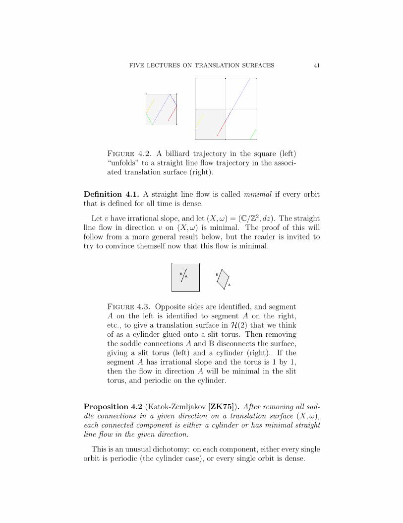
FIVE LECTURES ON TRANSLATION SURFACES 41
Figure 4.2. A billiard trajectory in the square (left)“unfolds” to a straight line flow trajectory in the associ-ated translation surface (right).
Definition 4.1. A straight line flow is called minimal if every orbitthat is defined for all time is dense.
Let v have irrational slope, and let (X,ω) = (C/Z2, dz). The straightline flow in direction v on (X,ω) is minimal. The proof of this willfollow from a more general result below, but the reader is invited totry to convince themself now that this flow is minimal.
Figure 4.3. Opposite sides are identified, and segmentA on the left is identified to segment A on the right,etc., to give a translation surface in H(2) that we thinkof as a cylinder glued onto a slit torus. Then removingthe saddle connections A and B disconnects the surface,giving a slit torus (left) and a cylinder (right). If thesegment A has irrational slope and the torus is 1 by 1,then the flow in direction A will be minimal in the slittorus, and periodic on the cylinder.
Proposition 4.2 (Katok-Zemljakov [ZK75]). After removing all sad-dle connections in a given direction on a translation surface (X,ω),each connected component is either a cylinder or has minimal straightline flow in the given direction.
This is an unusual dichotomy: on each component, either every singleorbit is periodic (the cylinder case), or every single orbit is dense.
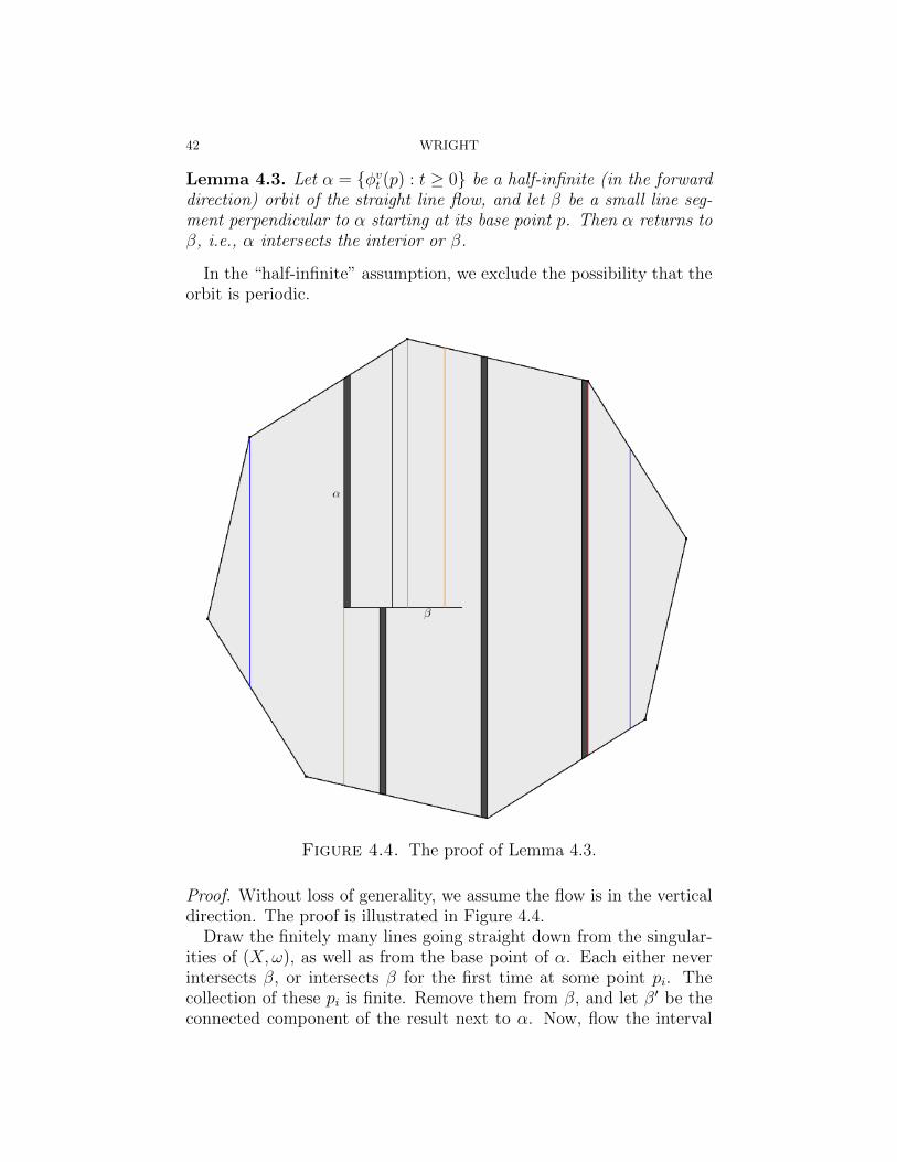
42 WRIGHT
Lemma 4.3. Let α = {φvt (p) : t ≥ 0} be a half-infinite (in the forwarddirection) orbit of the straight line flow, and let β be a small line seg-ment perpendicular to α starting at its base point p. Then α returns toβ, i.e., α intersects the interior or β.
In the “half-infinite” assumption, we exclude the possibility that theorbit is periodic.
Figure 4.4. The proof of Lemma 4.3.
Proof. Without loss of generality, we assume the flow is in the verticaldirection. The proof is illustrated in Figure 4.4.
Draw the finitely many lines going straight down from the singular-ities of (X,ω), as well as from the base point of α. Each either neverintersects β, or intersects β for the first time at some point pi. Thecollection of these pi is finite. Remove them from β, and let β′ be theconnected component of the result next to α. Now, flow the interval

FIVE LECTURES ON TRANSLATION SURFACES 43
β′ up to get rectangles ⋃t∈[0,T ]
φvt (β′)
of larger and larger height and hence larger and larger area. Sincethe area of the surface is finite, as T gets bigger the interval β′ musteventually come back to β. At this point we will see α intersect β,since once side of β′ is α.
The reason the pi were removed from β is to ensure that the rectangledoes not hit a singularity before returning to β, and so that when therectangle returns, it does not contain the base point of α. �
Proof of Proposition 4.2. Let C be the closure of a forward orbit of thestraight line flow in the given direction, which we will assume is vertical(i.e., in the “north” direction). It suffices to show that the boundary ofC consists of vertical saddle connections, if C is not a closed orbit. (Theinterior of C is then a connected component after removing all verticalsaddle connections, and the given orbit is dense in this component.)
Since C is closed and flow invariant, locally it looks like C ′×R, whereC ′ ⊂ R is a closed set. This C ′ is the complement of a union of disjointopen intervals. Let α be the vertical line segment through an endpointof one of these open intervals. Then α is in (the boundary of) C. Weassume, in order to find a contradiction, that α is at least half infinite(i.e., it is not a saddle connection). Without loss of generality, we willassume α is at least half infinite in the upwards direction.
By our choice of α, we can find some small horizontal segment βstarting at the base point of α whose interior is contained in the com-plement of C. However this contradicts the previous lemma, since α iscontained in C and must come back to the interior of β.
To conclude the argument, recall that C ′ is the complement of aunion of disjoint open intervals. We have shown that every endpointof these intervals is a saddle connection (i.e., not half infinite in eitherdirection). There are only finitely many horizontal saddle connections,so in fact C ′ is the complement of a finite union of open intervals.It follows that the boundary of C consists of saddle connections, asdesired. �
Proposition 4.4. On every (X,ω), the straight line flow is minimalin all but countably many directions.
Proof. There are only countably many saddle connections. In any di-rection that does not have saddle connections, the previous result saysthe straight line flow must be minimal. �
44 WRIGHT
4.2. Ergodicity. A measure preserving flow on a space Y with a prob-ability measure m is a homomorphism φ from R to the group of in-vertible measure preserving transformations from Y to itself. (Thesetransformations are typically only considered to be defined on set offull measure.)
Definition 4.5. A measure preserving flow on a space Y with prob-ability measure m is said to be ergodic if Y cannot be written as thedisjoint union of two subsets that are invariant under the flow, andeach of positive measure.
The flow is uniquely ergodic if m is the unique invariant measure forthe flow. (It follows that m is ergodic.)
Thus ergodicity is a basic indecomposability condition saying thatthe dynamics cannot be split into two smaller pieces (each of whichcould be studied separately). It is somewhat surprising that it im-plies the following strong restriction on the dynamics, whose proof isnontrivial but can be found in any book on ergodic theory.
Theorem 4.6 (Birkhoff Ergodic Theorem). Let φ be a measure pre-serving ergodic flow on a space Y with probability measure m, and letf ∈ L1(Y,m). Then, for m-almost every y ∈ Y ,
limT→∞
1
T
∫ T
0
φt(y)dt =
∫Y
fdm.
You should think of the case where f = χA is the characteristicfunction of a set A. Then the theorem says that long orbit segments{φt(y) : t ∈ [0, T ]} spend about m(A) of their time in A. Thusthe Birkhoff Ergodic Theorem says that almost every orbit is equidis-tributed, in that
limT→∞
1
TLeb({t : t ∈ [0, T ], φt(y) ∈ A})→ m(A),
where Leb denotes Lebesgue measure on R and A ⊂ Y is any measur-able set. (Technically, to be true as stated, some additional restrictionmust be place on A, for example, A is open. Otherwise any given orbitcan be removed from any measurable set A, giving a set A′ often ofthe same measure of A, but which the given orbit does not intersect atall.)
Proposition 4.7. Let φ be a uniquely ergodic flow on a compact spaceY with measure m. Then for every continuous f : Y → R, and everyy ∈ Y ,
limT→∞
1
T
∫ T
0
φt(y)dt =
∫Y
fdm.

FIVE LECTURES ON TRANSLATION SURFACES 45
It follows that, in the uniquely ergodic case, every orbit is equidis-tributed.
Recall the definition of weak-∗ convergence of measures on a compactspace Y : measures mn converge weak-∗ to m if, for all continuousfunctions f : Y → R, ∫
fdmn →∫fdm.
Proof. Let m be the unique invariant measure. Let mp,T be the pushforward of Lebesgue probability measure on [0, T ] via the map t 7→φt(p). Thus mp,T is Lebesgue probability measure along an orbit seg-ment. Let m′ be any weak-∗ limit of the mp,T . Notice the overlapbetween the orbit segment and the orbit segment translated by 1
φ∗1(mp,T )−mp,T =1
T
(mφ−1(p),1 −mφT−1(p),1
).
Since this converges to 0 weak-∗ as T → ∞, we see that m′ must beφ1 invariant, and similarity φ invariant (i.e., φt invariant for all t).
Since there is a unique invariant measure, m = m′. Thus Lebesgueprobability measure on longer and longer orbit segments {φt(y) : t ∈[0, T ]} converges weak-∗ to m, which is exactly what we wanted toshow. �
Renormalization of straight line flow. Say that the gt-orbit
{gt(X,ω), t ≥ 0}is recurrent if there is some compact set K of the stratum, such thatgt(X,ω) ∈ K for arbitrarily large t. This exactly says that gt(X,ω)does not diverge to infinity.
Given an orbit segment of vertical straight line flow on (X,ω) oflength L, it yields an orbit segment of vertical straight line flow ongt(X,ω) of length e−tL. In this way long orbit segments of verticalstraight line flow become small under gt, and we say that gt renor-malizes the vertical straight line flow. This idea of replacing a longorbit segment of a dynamical segment for a shorter orbit segment of adifferent but related dynamical system is called renormalization, andis fundamental in dynamics. For the straight line flow, it was used toprove the following.
Theorem 4.8 (Masur’s criterion [Mas92]). Suppose that gt(X,ω) isrecurrent. Then the vertical straight line flow on (X,ω) is uniquelyergodic.
The converse is not true, however the result is extremely powerful.

46 WRIGHT
Theorem 4.9 (Kerkhoff-Masur-Smillie [KMS86]). For every (X,ω)and almost every θ ∈ [0, 2π), gt(rθ(X,ω)) is recurrent (as θ is fixedand t→∞). Thus, for every (X,ω), the straight line flow is uniquelyergodic in almost every direction.
This implies the same result for billiard flows in rational polygons.This was one of the most spectacular early successes in the field.
Remark 4.10. There exist (X,ω) such that the vertical flow is minimalbut not uniquely ergodic. This is a bit strange; every orbit is dense, butmost orbits are not equidistributed, and hence somehow favor (spendmore time than expected in) some parts of (X,ω).
4.3. Complete periodicity. The dynamics are much more restrictedfor (X,ω) that lie in a 2-dimensional affine invariant submanifold. Such(X,ω) are called lattice surfaces, since their stabilizer is a lattice inSL(2,R).
Theorem 4.11 (Veech dichotomy [Vee89]). For any lattice surface,in the direction of any saddle connection the surface is periodic. In allother directions the straight line flow is uniquely ergodic.
This is the same dichotomy that holds for (C/Z2, dz), where theflow is periodic in the rational directions, and uniquely ergodic in theirrational directions.
The proof of the following lemma is easy, but it will be omitted,because it requires familiarity with the geodesic flow on a finite volumecomplete hyperbolic surface (every geodesic is either recurrent, or iteventually goes straight out a cusp, and the action of gt on SL(2,R)/Γis geodesic flow on the unit tangent bundle to a hyperbolic surface).
Lemma 4.12. For lattice surface (X,ω), either gt(X,ω) is recurrent,or (X,ω) is stabilized by some matrix(
1 0s 1
)with s 6= 0.
Proof of Veech dichotomy. It suffices to prove the statement for the ver-tical direction (since the surface can be rotated to make any directionvertical).
By the lemma, either gt(X,ω) is recurrent, or (X,ω) is stabilized bythe matrix above. In the first case, Masur’s criterion gives that theflow is uniquely ergodic (and it is easy to see there can be no verticalsaddle connections, or else gt(X,ω) would diverge). In the second case,Proposition 3.5 gives that the surface is the union of vertical cylinders

FIVE LECTURES ON TRANSLATION SURFACES 47
(and so there are vertical saddle connections, on the boundary of thecylinders). �
We will also give a more modern proof of just the first statement,together with a generalization. For this we will need
Theorem 4.13 (Minsky-Weiss, Smillie-Weiss [MW02,SW04]). Theut-orbit closure of any (X,ω) contains a horizontally periodic surface.
Recall ut =
(1 t0 1
).
Lemma 4.14. For any horizontal cylinder or saddle connection on(X,ω), and each t, there is a corresponding horizontal cylinder or sad-dle connection on ut(X,ω).
Furthermore, there is a corresponding horizontal cylinder or unionof horizontal saddle connections on each translation surface (X ′, ω′) inthe ut-orbit closure of (X,ω).
Proof. The first statement follows because the matrix ut fixes the hor-izontal direction. Now consider (X ′, ω′) = limn→∞ utn(X,ω). For eachhorizontal cylinder on (X,ω), there is a corresponding horizontal cylin-der on each utn(X,ω), and hence there is also a horizontal cylinder inthe limit.
The same argument applies equally well to horizontal saddle con-nections, except that possibly in the limit a zero could “land” on theinterior of the saddle connection, subdividing it into several horizontalsaddle connections. �
Proposition 4.15 (One part of the Veech dichotomy). Suppose (X,ω)is a lattice surface, and has a horizontal saddle connection. Then(X,ω) is horizontally periodic.
Proof. Let (X ′, ω′) be horizontally periodic and in the ut(X,ω)-orbitclosure of (X,ω). Let T be large, so uT (X,ω) is very close to (X ′, ω′).The horizontal saddle connection is present on (X ′, ω′) as a union ofhorizontal saddle connections (it will turn out to be only one). Theremust be some matrix g ∈ SL(2,R) close to the identity so guT (X,ω) =(X ′, ω′), because they are both in the same orbit. Also, g must preservethe horizontal direction, since it must preserve the horizontal saddleconnections. However, that means g is a unipotent upper triangularmatrix g = uS, so uT+S(X,ω) is horizontally periodic, so (X,ω) ishorizontally periodic. �
Definition 4.16. A rel deformation of translation surface is a path(Xt, ωt), t ∈ [a, b], in a stratum, such that for any absolute homologyclass γ,
∫γωt is constant.

48 WRIGHT
Thus along rel deformations absolute periods are constant, but rela-tive periods (i.e., the complex distance between zeros of ω) can change.
Figure 4.5. The translation surface on the right andthe one on the left are rel deformations of each other.More generally, changing the length of the slit in the slittorus construction gives a rel deformation. It is possibleto write down a basis for absolute homology consisting ofcycles disjoint from the slit, which shows that the integralof any absolute homology class does not change as thecomplex length of the slit is changed.
Figure 4.6. Opposite edges are identified (the bottomedges each consist of two saddle connections), giving twosurfaces in H(1, 1). The translation surface on the rightand the surface on the left are rel deformations of eachother. The surface on the right was obtained from theone on the left by subtracting 1 from the height of thebottom cylinder, and adding 1 to the height of the twotop cylinders.
Example 4.17. If (X ′, ω′) is a translation cover of (X,ω), then mov-ing the branch points gives a rel deformation of (X ′, ω′), consistingentirely of surfaces that cover (X,ω). (Compare to the computationsin example 2.2.)
Lemma 4.18. Suppose that (X,ω) and (X ′, ω′) are nearby surfaces insome stratum, and as subspaces of absolute cohomology H1(X,C) wehave
spanR(Re(ω), Im(ω)) = spanR(Re(ω′), Im(ω′)).

FIVE LECTURES ON TRANSLATION SURFACES 49
Then there is some g ∈ GL+(2,R) close to the identity such thatg(X ′, ω′) is a rel deformation of (X,ω).
Proof. By assumption, there are constants a, b, c, d ∈ R such that, inabsolute cohomology,
Re(ω′) = aRe(ω) + b Im(ω) and Im(ω′) = cRe(ω) + d Im(ω).
Thus if
g =
(a bc d
),
then g(X,ω) and (X ′, ω′) have the same absolute periods, and henceare rel deformations of each other. In particular, the linear path inlocal periods joining g(X,ω) and (X ′, ω′) is a rel deformation. �
Definition 4.19. An affine invariant submanifold M is rank 1 if,for every (X,ω) ∈ M, there is an open neighbourhood U contain-ing (X,ω), such that for every (X ′, ω′) ∈ U there is a g ∈ GL+(2,R)close to the identity such that there is a rel deformation in U from(X ′, ω′) to g(X,ω).
A definition of rank will be given in the next lecture, so this can beconsidered a provisional definition of rank 1. It can be rephrased as say-ing that the GL+(2,R) directions and the directions of rel deformationsin M span the tangent space to M at every point. By the previouslemma, it can also be rephrased as saying that span(Re(ω), Im(ω)) islocally constant on M.
Proposition 4.20. Let M be a 2-dimensional affine invariant sub-manifold. Then M is rank 1. Furthermore, let M′ be a connectedcomponent of the space of degree d translation covers of surfaces in Mbranched over k points. Then M′ is rank 1 also.
Proof. A 2-dimensional affine invariant submanifoldM is a singleGL+(2,R)-orbit, and so is in particular rank 1 (the rel deformations aren’t evenrequired).
If (X ′, ω) ∈ M′ is a cover of (X,ω) ∈ M, then a neighborhood inM′ of (X ′, ω′) is obtained by changing (X,ω) by a small matrix inGL+(2,R), and changing the location of the branch points. �
Proposition 4.21. The eigenform loci in genus two constructed in thesecond lecture are rank 1.
Proof. These are defined by saying that the real and imaginary partsof ω should span a fixed 2-dimensional subspace of absolute homology(the
√D-eigenspace of M). �

50 WRIGHT
Proposition 4.22 (Wright). If (X,ω) ∈ M and M is rank 1, then(X,ω) is periodic in any direction that has a cylinder.
That is, the proposition says that every time you find a cylinder on(X,ω), then (X,ω) is the union of that cylinder and cylinders parallelto it. Before being established in general in [Wria] (using a differentargument than the one we give here), the proposition was known inseveral special cases [Vee89,Cal04,LN].
Proof. Let (X ′, ω′) be horizontally periodic and in the ut-orbit closureof (X,ω).
Let T be large, so uT (X,ω) is very close to (X ′, ω′). The hori-zontal cylinder is present on (X ′, ω′). There must be some matrixg ∈ SL(2,R) close to the identity so guT (X,ω) is a rel deformation of(X ′, ω′). Small rel deformations preserve cylinders, since the integralover their circumference curve γ must remain constant along the reldeformation. Hence g must preserve the horizontal direction, since itmust preserve the horizontal cylinder which is present on both uT (X,ω)and guT (X,ω).
Thus, every horizontal cylinder on (X ′, ω′) is also horizontal onuT (X,ω). If these cylinders do not cover uT (X,ω), then it is possibleto derive a contradiction, because then there would be more horizontalcylinders on (X ′, ω′). (Because every horizontal cylinder on uT (X,ω)must also be present on every translation surface in the ut-orbit closure,and if they do not cover uT (X,ω) then the corresponding cylinders on(X ′, ω′) do not cover (X ′, ω′), and hence there must be more cylinderson (X ′, ω′) than on (X,ω).) �
Remark 4.23. In fact this proof shows that if (X,ω) has a loop γ ofsaddle connections in a fixed direction, and
∫γω 6= 0, then (X,ω) is
periodic in that direction.
We conclude by remarking that there is also a close connection be-tween rank 1 orbit closures and real multiplication. The proof requiresdynamics.
Theorem 4.24 (Filip). If (X,ω) ∈M andM is rank 1, then Jac(X,ω)has real multiplication.
The conclusion is that rank 1 orbit closures are very close cousins to2-dimensional orbit closures, which are a special case.
Exercises.(1) Depending on the stratum, what is the maximum number of par-
allel cylinders a translation surface can have? First argue in H(2)and H(1, 1).

FIVE LECTURES ON TRANSLATION SURFACES 51
Figure 4.7. This is a picture of some of the differentaspects translation surfaces and related fields.
(2) Using the slit torus construction, give an example of a genus threetranslation surface with three minimal components in some direc-tion.
(3) It is known that the action of gt is ergodic on the set of unit areasurfaces in each affine invariant submanifold. Using this and theBirkhoff Ergodic Theorem, show that almost every surface in anaffine invariant submanifold has full GL+(2,R)-orbit closure.
(4) Prove that every translation surface has a cylinder.(5) For the M′ in Proposition 4.20, derive Proposition 4.22 from the
Veech dichotomy for (X,ω) ∈ M, but show that the Veech Di-chotomy itself need not hold.
(6) Research problem: Classify rank 1 affine invariant submanifoldsM for which Jac(X,ω) = Jac(X) and M is closed under rel de-formations in the stratum (so M “has all the rel”). It is knownthat in each genus g > 2 there are at most finitely many [MW],

52 WRIGHT
but currently zero examples are known besides closed orbits in theminimal stratum. (In a stratum with s zeros, such an M musthave dimension 2 + s− 1.)
5. Revisiting genus two with new tools
5.1. Field of definition, VHS.
Definition 5.1. The (affine) field of definition k(M) of an affine in-variant submanifoldM is the smallest subfield of R such thatM can bedefined in local period coordinates by linear equations with coefficientsin this field [Wrib]. Warning: This is not the same thing as the fieldof definition ofM viewed as a variety (where polynomial equations areallowed, and the coordinates are different).
For example, M arising from branched covers over tori, (or over allsurfaces in some other stratum) are defined over Q. The eigenform loci
are defined over Q[√D].
Let H1 denote the flat bundle overM whose fiber over (X,ω) ∈Mis H1(X,C), and let H1
rel denote the flat bundle whose fiber over (X,ω)is H1(X,Σ,C), where Σ is the set of singularities of (X,ω). Let
p : H1rel → H1
denote the natural projection from relative to absolute cohomology.Viewing
H1(X,Σ,C) = H1(X,Σ,C)∗ and H1(X,C) = H1(X,C)∗,
the map p is just restriction of a linear functional on H1(X,Σ,C) toH1(X,C) ⊂ H1(X,Σ,C). The subspace ker(p) exactly corresponds toderivatives of rel deformations.
The flat connection on H1 or H1rel is often called the Gauss-Manin
connection. From our point of view, it is an extremely simple thing.The cohomology groups H1(X,C) and H1(X,Σ,C) are both purelytopological objects, and do not depend on the complex structure on Xor the Abelian differential ω. (When the Abelian differential changes,the set Σ might move a bit by an isotopy.) Thus, varying the complexstructure on X does not change these cohomology groups. In this way,if (X ′, ω′) is nearby (X,ω), then H1(X,C) is identified with H1(X ′, ω′)(because it is the same exact object!), and similarly for relative coho-mology. This identification of nearby fibers is exactly the structure ofa flat connection.
Recall that period coordinates can be considered as the map send-ing (X,ω) to the relative cohomology class of ω in H1(X,Σ,C). Bydefinition, M is defined in these periods by a linear subspace, which

FIVE LECTURES ON TRANSLATION SURFACES 53
we think of as simultaneously giving M in period coordinates, as wellas being the tangent space to M at (X,ω). (The tangent space to avector space, at any point, is just the vector space itself.) Thus we canconsider the tangent bundle T (M) of M as a flat subbundle of H1
rel.It is flat because the subspace defining M in period coordinates doesnot change as (X,ω) moves around in M.
A flat subbundle E of H1 or H1rel is just a subbundle that is locally
constant over M. Associated to such a subbundle is its monodromyrepresentation, which is a representation of π1(M) on a fiber of E atthe chosen base point of M. It is obtained by dragging cohomologyclasses around loops in π1(M).
A flat subbundle is called simple if it has no nontrivial flat subbun-dle, or equivalently if the monodromy representation has no nontrivialinvariant subspaces. A flat subbundle is called semisimple if it is thedirect sum of simple subbundles. Two subbundles are called Galoisconjugate if their fibers are Galois conjugate; in particular, this meanstheir monodromy representations are Galois conjugate.
Definition 5.2. The field of definition of a flat subbundle E ⊂ H1 isthe smallest subfield of C such that locally the linear subspace E ofH1(X,C) can be defined by linear equations (with respect to an integerbasis of H1(X,Z)) with coefficients in this field. The trace field of aflat bundle over M is defined as the field generated by traces of thecorresponding representation of π1(M).
Theorem 5.3 (Wright [Wrib]). LetM be an affine invariant subman-ifold. The field of definition of p(T (M)) and trace field of p(T (M))are both equal to k(M).
Set VId = p(T (M)). There is a semisimple flat bundle W, and foreach field embedding ρ : k(M) → C there is a flat simple bundle Vρ
that is Galois conjugate to VId, such that
H1 =
(⊕ρ
Vρ
)⊕W.
The bundle W does not contain any subbundles isomorphic to anyVρ. Both W and ⊕Vρ are defined over Q. All direct summands aresymplectic and symplectically orthogonal.
In particular,
dimC p(T (M)) · degQ k(M) ≤ 2g.
Corollary 5.4 (Wright). In particular, the field of definition is a num-ber field, and so any translation surface whose coordinates are linearlyindependent over Q cannot be contained in a nontrivial affine invariant

54 WRIGHT
submanifold, and hence must have GL+(2,R)-orbit closure as large aspossible. This provides an explicit full measure set of surfaces whoseorbit closure is as large as possible.
The direct sum decomposition of H1 in Theorem 5.3 was previ-ously established in the case of Teichmuller curves by Martin Moller[Mol06b], and is one of the main tools used in the study of closedSL(2,R)–orbits.
Theorem 5.5 (Moller [Mol06b], Filip [Filb]). The splitting aboveis a splitting of Variation of Hodge Structures. That is, each directsummand is equal to the direct sum of its intersection with H1,0 andits intersection with H0,1.
Again the proofs use dynamics. For an elementary introductionof Variation of Hodge Structures in the context of orbit closures, see[Wri12].
When the splitting of H1 is nontrivial (H1 6= p(T (M))), then Mparameterizes translation surfaces whose Jacobians admit nontrivialendomorphisms.
Given that affine invariant submanifolds are varieties, parts (butnot all) of the two theorems above follow from a theorem of Deligneon semi-simplicity of VHS [Del87]. However, in fact both the abovetheorems were established first, and used by Filip in his proof that affineinvariant submanifolds are varieties. The first theorem used work ofAvila-Eskin-Moller [AEM], and the following.
Theorem 5.6 (Eskin-Mirzakhani-Rafi [EMR]). In every affine in-variant submanifolds, there are lots of closed (i.e., periodic) gt-orbits.
This is useful because of a classical result in Teichmuller theory thatsays the monodromy matrix over such an orbit has simple largest andsmallest eigenvalues, with eigenvectors Re(ω) and Im(ω). Among otherthings, this helps to show that there is not a second copy of p(T (M))in the decomposition of H1, since otherwise these eigenvalues wouldhave multiplicity at least two.
The work of Avila-Eskin-Moller used in the proof also shows
Theorem 5.7 (Avila-Eskin-Moller). p(T (M)) is symplectic.
Definition 5.8. The rank of an affine invariant submanifold M is12
dimC p(T (M)).
When p(T (M)) is 2-dimensional, that means that it must be spannedby the real and imaginary parts of the absolute cohomology classesgiven by ω. In particular, span(Re(ω), Im(ω)) is locally constant, since

FIVE LECTURES ON TRANSLATION SURFACES 55
p(T (M)) is always a flat subbundle. By Lemma 4.18, this means thata neighbourhood of any (X,ω) inM can be generated using GL+(2,R)and rel deformations, so rank 1 according to this definition agrees withour previous definition of rank 1.
5.2. Cylinder deformations. We begin with the observation that,for each cylinder on a translation surface (X,ω), there is a correspond-ing cylinder on sufficiently nearby surfaces (X ′, ω′). This correspond-ing cylinder may not have the same direction, height, circumference,or modulus, however these all change continuously with (X ′, ω′). The“sufficiently nearby” assumption is required since, along a path a sur-faces starting at (X,ω), the height of the cylinder might reach 0, atwhich point the cylinder ceases to be a cylinder.
Figure 5.1. Consider the shaded horizontal cylinder onthe regular octagon surface in H(2) (left). On any suf-ficiently small deformation of this surface, the cylinderpersists (right).
Definition 5.9. Two cylinders C1 and C2 on (X,ω) ∈M are said to beM-parallel if they are parallel, and remain parallel on all deformationsof (X,ω) inM. (A deformation is just a nearby surface, connected to(X,ω) via a path in M.) The deformations are assumed to be small,so that C1 and C2 persist.
Example 5.10. IfM is 2-dimensional, it consists of a singleGL+(2,R)-orbit. Parallel cylinders remain parallel under the action of GL+(2,R),so two cylinders on a translation surface in M are M-parallel if andonly if they are parallel.
Example 5.11. On the opposite extreme, if M is a connected com-ponent of a stratum, two cylinders are M parallel if and only if theyare parallel and their circumference curves are homologous. Indeed,suppose the core curves are γ1 and γ2. Then since
∫γ1ω′ =
∫γ2ω′ on all
deformations (X ′, ω′) ∈ M, the cylinders will always be in the samedirection, which is exactly the direction in C given by this integral.

56 WRIGHT
Figure 5.2. The two shaded cylinders are homologouson this translation surface. There is no way to deformthe surface to make these two cylinders not be parallel.
Lemma 5.12. Two cylinders C1 and C2 on (X,ω) ∈M areM-parallelif and only if there is a constant c ∈ R such that on all deformations(X ′, ω′) ∈M, ∫
γ1
ω′ = c
∫γ2
ω′,
where γi is the circumference curve of Ci.
In other words, two cylinders on (X,ω) ∈ M are M-parallel if andonly if one of the linear equations defining M in local period coordi-nates makes it so.
Proof. Both (X ′, ω′) 7→∫γ1ω′ and (X ′, ω′) 7→
∫γ2ω′ are linear function-
als on a neighbourhood of (X,ω) in M, viewed in period coordinatesas locally being an open set in a complex vector space. The cylindersC1, C2 areM parallel if and only if these two linear functions are alwaysreal multiples of each other.
The only way for two linear functionals on a complex vector spacealways have real ratio is for one functional to be a fixed real constantc times the other. �
The relation of beingM-parallel is an equivalence relation, and whenwe speak of an equivalence class of a cylinder, we mean the set of allcylinders M-parallel to it.
Define the matrices
ut =
(1 t0 1
), as =
(1 00 es
), rθ =
(cos θ − sin θsin θ cos θ
).
Let C be a collection of parallel cylinders on a translation surface (X,ω).Suppose they are all of angle θ ∈ [0, π). Define aCs (u
Ct (X,ω))) to be the
translation surface obtained by applying r−θ to (X,ω), then applying

FIVE LECTURES ON TRANSLATION SURFACES 57
the matrix asut to the images of the cylinders in C, and then applyingrθ.
The result of aCs is to stretch the height of all cylinders in the collec-tion C by a factor of es. The result of uCt is to shear all the cylindersin C.
Figure 5.3. A horizontal cylinder (left–vertical sidesare identified, but the top and bottom horizontal edgesare the boundary of the cylinder.) The result of stretch-ing and shearing this cylinder (right). Note the boundaryof the cylinder stays exactly the same.
There is more than one way of thinking about these cylinder defor-mations. You can think of cutting out the cylinders in C, and thenstretching and shearing them, and then gluing them back in. Or, youcan think of a polygon decomposition for (X,ω), with one parallelo-gram for each cylinder in C, and you can think of applying the matrixasut just to the parallelograms giving cylinders in C and doing nothingto the remaining polygons.
Figure 5.4. On the left is a translation surface (X,ω).Let C be the two shaded parallel cylinders on (X,ω). Onthe right is aClog(2)(X,ω).
Theorem 5.13 (The Cylinder Deformation Theorem [Wria]). Sup-pose that C is an equivalence class of M-parallel cylinders on (X,ω) ∈M. Then for all s, t ∈ R, the translation surface aCs (u
Ct (X,ω)) ∈M.
We call aCs the cylinder stretch, and uCt the cylinder shear.The proof involves the dynamics of ut, but is motivated by the then
conjecture (now theorem) that affine invariant submanifolds are va-rieties. As s → ∞, the translation surface aCs (C(X,ω)) converges to

58 WRIGHT
the boundary at infinity ofM. The Cylinder Deformation Theorem isclosely related to the boundary structure of M.
More generally, the boundary of an affine invariant submanifold isrelated to configurations of parallel cylinders and saddle connections,since these can always be made vertical using rθ and then shrunk usinggt.
5.3. Orbit closures in genus 2. McMullen classified orbit closuresin H(2) and H(1, 1) [McM07]. We will now recover some qualitativeaspects of this classification using the machinery of the last two subsec-tions. (Many of the finer aspects of the work in genus two by McMullenand his students, for example [McM05,McM06b,McM03b,Bai07,Mukb], cannot be proved quickly, even with new tools.)
Lemma 5.14. In H(2) every GL+(2,R)-orbit is dense or closed. Everyclosed orbit is either the orbit of a square-tiled surface, or one of theeigenform loci in H(2) constructed in lecture 2.
Even the orbits of square-tiled surfaces can be fit into the frameworkof eigenforms by considering “real multiplication by Q⊕Q”, but we donot pursue that perspective here.
Proof. Every orbit closure is an affine invariant submanifold. In stratawith only one zero, p : H1(X,Σ,C) → H1(X,C) is an isomorphism,and hence T (M) = p(T (M) is symplectic. Hence becauseM⊂ H(2),we see thatM is 2-dimensional or 4-dimensional. H(2) is 4-dimensionaland connected, so any 4-dimensional affine invariant submanifold is allof H(2).
Thus we may assume that M is 2-dimensional, i.e., a closed orbit.If M is defined over Q, it contains surface (X,ω) whose periods{∫
γ
ω : γ ∈ H1(X,Z)
}⊂ 1
nZ2
for some n. It follows from an exercise in these notes thatM containsa square-tiled surface (a cover of C/( 1
nZ2)).
If M is defined over Q[√D], then it follows from Theorem 5.3 that
span(Re(ω), Im(ω))
is defined over Q[√D] and is symplectically orthogonal to the Galois
conjugate subspace. Hence by lecture 2, (X,ω) is an eigenform for real
multiplication by an order in Q[√D]. �
Similarly we obtain
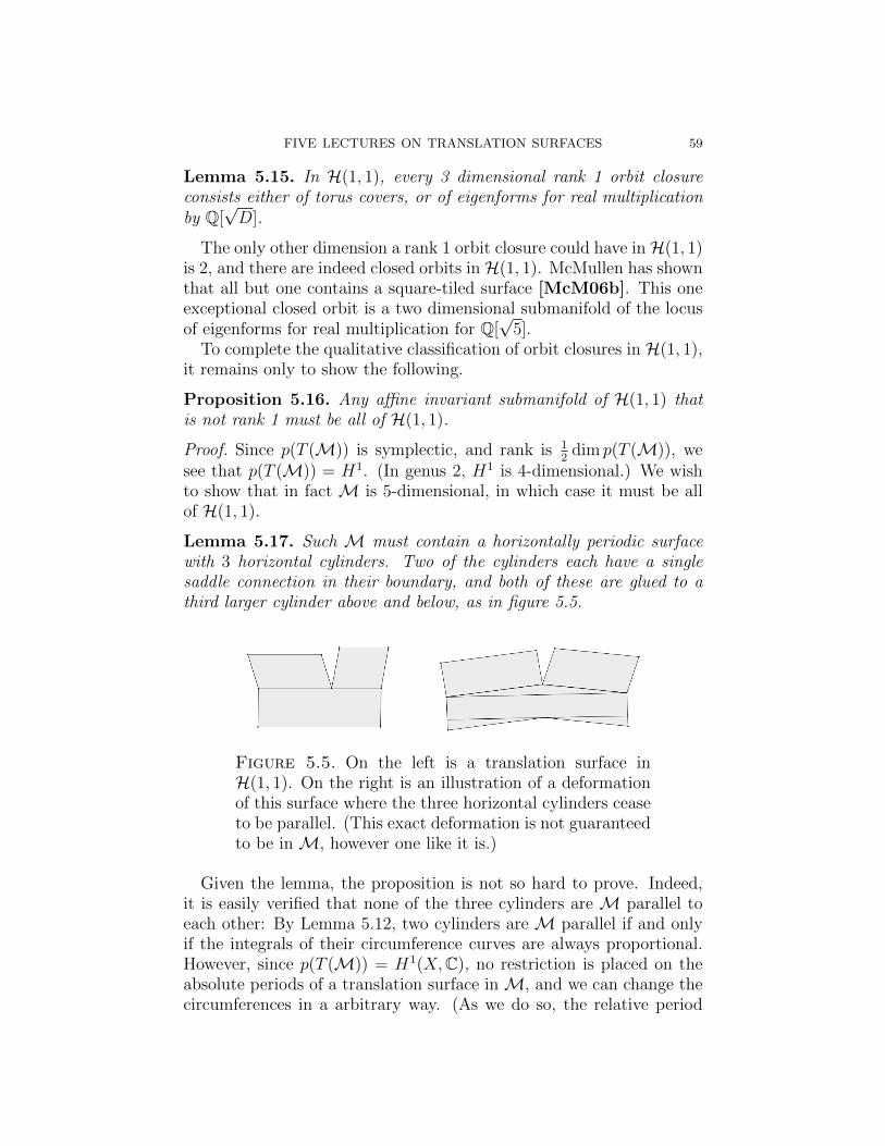
FIVE LECTURES ON TRANSLATION SURFACES 59
Lemma 5.15. In H(1, 1), every 3 dimensional rank 1 orbit closureconsists either of torus covers, or of eigenforms for real multiplicationby Q[
√D].
The only other dimension a rank 1 orbit closure could have inH(1, 1)is 2, and there are indeed closed orbits in H(1, 1). McMullen has shownthat all but one contains a square-tiled surface [McM06b]. This oneexceptional closed orbit is a two dimensional submanifold of the locusof eigenforms for real multiplication for Q[
√5].
To complete the qualitative classification of orbit closures in H(1, 1),it remains only to show the following.
Proposition 5.16. Any affine invariant submanifold of H(1, 1) thatis not rank 1 must be all of H(1, 1).
Proof. Since p(T (M)) is symplectic, and rank is 12
dim p(T (M)), wesee that p(T (M)) = H1. (In genus 2, H1 is 4-dimensional.) We wishto show that in fact M is 5-dimensional, in which case it must be allof H(1, 1).
Lemma 5.17. Such M must contain a horizontally periodic surfacewith 3 horizontal cylinders. Two of the cylinders each have a singlesaddle connection in their boundary, and both of these are glued to athird larger cylinder above and below, as in figure 5.5.
Figure 5.5. On the left is a translation surface inH(1, 1). On the right is an illustration of a deformationof this surface where the three horizontal cylinders ceaseto be parallel. (This exact deformation is not guaranteedto be in M, however one like it is.)
Given the lemma, the proposition is not so hard to prove. Indeed,it is easily verified that none of the three cylinders are M parallel toeach other: By Lemma 5.12, two cylinders are M parallel if and onlyif the integrals of their circumference curves are always proportional.However, since p(T (M)) = H1(X,C), no restriction is placed on theabsolute periods of a translation surface inM, and we can change thecircumferences in a arbitrary way. (As we do so, the relative period

60 WRIGHT
might be determined by the absolute ones–but this is precisely whatwe will show cannot happen, since M will end up being H(1, 1).)
Since none of the three cylinders are M parallel to each other, wecan increase the height of top two, and decrease the height of thebottom one, so as to produce a rel deformation in M, as in figure4.6. Since p(T (M)) = H1(X,M), and T (M) contains a vector inthe 1-dimensional ker(p) (the rel deformation), we see that T (M) =H1(X,Σ,C). Hence M is 5-dimensional, and M = H(1, 1). �
The proof of Lemma 5.17 is easy but will be omitted. (One can finda horizontally periodic surface in every horocycle flow orbit closure,and work from there to get one with three horizontal cylinders. Seefigure 5.6, and compare to arguments in [NW,ANW].)
Figure 5.6. The proof of Lemma 5.17 is omitted, butthis figure gives the idea. On the left is a translationsurface with two horizontal cylinders. Shearing the twoshaded nonhorizontal cylinders appropriately “opposite”amounts gives the surface on the right, which now hasthree horizontal cylinders as desired.
5.4. Census of known orbit closures. Here we give a list of the cur-rently known orbit closures not arising from the elementary construc-tions discussed in Section 2.1. We give only primitive orbit closures,i.e., those not arising from covering constructions.
Closed orbits. McMullen and Calta independently discovered infin-itely many closed orbits in H(2) [Cal04, McM03a]. McMullen gen-eralized his approach using real multiplication to find infinitely manyprimitive closed orbits in genus 3 and 4, in the Prym loci in the stratawhere ω has only one zero [McM06a].
There is a bi-infinite sequence of Teichmuller curves T (n,m) calledthe Veech-Ward-Bouw-Moller curves. For n = 2 they were discoveredby Veech [Vee89]; for n = 3 by Ward [War98]; and in the general

FIVE LECTURES ON TRANSLATION SURFACES 61
case by Bouw and Moller [BM10]. They have also been studied bythe author and Hooper [Wri13,Hoo].
There are also two “sporadic” closed orbits known, one due to Voro-bets in H(6), and another due to Kenyon-Smillie in H(1, 3) [HS01,KS00]. These sporadic examples correspond to billiards in the (π/5, π/3, 7π/15)and (2π/9, π/3, 4π/9) triangles respectively.
Rank 1 affine invariant manifolds. McMullen and Calta discov-ered infinitely many rank 1 affine invariant submanifolds in H(1, 1)[Cal04,McM03a]. McMullen generalized his construction to give in-finitely many additional examples in the Prym loci in genus 3, 4, and5 [McM06a].
A new orbit closure. In joint work in progress with Mirzakhani,the author has found the first known example of a higher rank orbitclosure whose affine field of definition is not Q.
Exercises.(1) If (X,ω) has only one singularity, then (X,ω) does not have any
homologous pairs of cylinders.(2) Show that the field of definition is well defined, and that it is the
field generated by the coefficients of the rref of any system of equa-tions defining the subspace. Hint: first figure out the field of defi-nition of a line in C2.
(3) Show that any rank 1 affine invariant submanifold defined over Qconsists entirely of branched covers of tori.
(4) Prove that the eigenform loci are dense in H(2), and in in H(1, 1).(You will probably need to use the big technology presented inthese lectures.)
(5) Show that if a horizontally periodic translation surface has cylin-ders with moduli linearly independent over Q, then there is a cylin-der deformation contained in its horocycle flow orbit closure.
(6) Prove there is no 3-dimensional orbit closure in H(4).(7) Research problem: Is there a cubic rank 3 of dimension 3 in genus
three?
References
[AEM] Artur Avila, Alex Eskin, and Martin Moller, Symplectic and Isomet-ric SL(2,R)-invariant subbundles of the Hodge bundle, preprint, arXiv1209.2854 (2012).
[ANW] David Aulicino, Duc-Manh Nguyen, and Alex Wright, Classification ofhigher rank orbit closures in Hodd(4), preprint, arXiv 1308.5879 (2013),to appear in Geom. Top.

62 WRIGHT
[Bai07] Matt Bainbridge, Euler characteristics of Teichmuller curves in genustwo, Geom. Topol. 11 (2007), 1887–2073.
[BM10] Irene I. Bouw and Martin Moller, Teichmuller curves, triangle groups,and Lyapunov exponents, Ann. of Math. (2) 172 (2010), no. 1, 139–185.
[BM12] Matt Bainbridge and Martin Moller, The Deligne-Mumford compactifi-cation of the real multiplication locus and Teichmuller curves in genus3, Acta Math. 208 (2012), no. 1, 1–92.
[Cal04] Kariane Calta, Veech surfaces and complete periodicity in genus two, J.Amer. Math. Soc. 17 (2004), no. 4, 871–908.
[Del87] P. Deligne, Un theoreme de finitude pour la monodromie, Discretegroups in geometry and analysis (New Haven, Conn., 1984), Progr.Math., vol. 67, Birkhauser Boston, Boston, MA, 1987, pp. 1–19.
[DT02] Tobin A. Driscoll and Lloyd N. Trefethen, Schwarz-Christoffel mapping,Cambridge Monographs on Applied and Computational Mathematics,vol. 8, Cambridge University Press, Cambridge, 2002.
[EM] Alex Eskin and Maryam Mirzakhani, Invariant and stationary mea-sures for the SL(2,R) action on moduli space, preprint, arXiv 1302.3320(2013).
[EM01] Alex Eskin and Howard Masur, Asymptotic formulas on flat surfaces,Ergodic Theory Dynam. Systems 21 (2001), no. 2, 443–478.
[EMM] Alex Eskin, Maryam Mirzakhani, and Amir Mohammadi, Isolation the-orems for SL(2,R)-invariant submanifolds in moduli space, preprint,arXiv:1305.3015 (2013).
[EMR] Alex Eskin, Maryam Mirzakhani, and Kasra Rafi, Counting closedgeodesics in strata, preprint, arXiv 1206.5574 (2012).
[Esk06] Alex Eskin, Counting problems in moduli space, Handbook of dynamicalsystems. Vol. 1B, Elsevier B. V., Amsterdam, 2006, pp. 581–595.
[Fila] Simion Filip, Semisimplicity and rigidity of the Kontsevich-Zorich cocy-cle, preprint, arXiv:1307.7314 (2013).
[Filb] , Splitting mixed Hodge structures over affine invariant mani-folds, preprint, arXiv:1311.2350 (2013).
[For06a] Giovanni Forni, On the Lyapunov exponents of the Kontsevich-Zorichcocycle, Handbook of dynamical systems. Vol. 1B, Elsevier B. V., Am-sterdam, 2006, pp. 549–580.
[For06b] , On the Lyapunov exponents of the Kontsevich-Zorich cocycle,Handbook of dynamical systems. Vol. 1B, Elsevier B. V., Amsterdam,2006, pp. 549–580.
[Hoo] W. Patrick Hooper, Grid graphs and lattice surfaces, preprint, arXiv0811.0799 (2009).
[HS01] P. Hubert and T. A. Schmidt, Invariants of translation surfaces, Ann.Inst. Fourier (Grenoble) 51 (2001), no. 2, 461–495.
[HS06] Pascal Hubert and Thomas A. Schmidt, An introduction to Veech sur-faces, Handbook of dynamical systems. Vol. 1B, Elsevier B. V., Ams-terdam, 2006, pp. 501–526.
[KM] Abhinav Kumar and Ronen E. Mukamel, Algebraic models and arith-metic geometry of Teichmuller curves in genus two, preprint, arXiv1406.7057 (2014).

FIVE LECTURES ON TRANSLATION SURFACES 63
[KMS86] Steven Kerckhoff, Howard Masur, and John Smillie, Ergodicity of billiardflows and quadratic differentials, Ann. of Math. (2) 124 (1986), no. 2,293–311.
[KS00] Richard Kenyon and John Smillie, Billiards on rational-angled triangles,Comment. Math. Helv. 75 (2000), no. 1, 65–108.
[LM14] Eduard Looijenga and Gabriele Mondello, The fine structure of the mod-uli space of abelian differentials in genus 3, Geom. Dedicata 169 (2014),109–128.
[LN] Erwan Lanneau and Duc-Mahn Nguyen, Complete periodicity of prymeigenforms, preprint, arXiv 1301.0783 (2013).
[Mas82] Howard Masur, Interval exchange transformations and measured folia-tions, Ann. of Math. (2) 115 (1982), no. 1, 169–200.
[Mas92] , Hausdorff dimension of the set of nonergodic foliations of aquadratic differential, Duke Math. J. 66 (1992), no. 3, 387–442.
[Mas06] , Ergodic theory of translation surfaces, Handbook of dynamicalsystems. Vol. 1B, Elsevier B. V., Amsterdam, 2006, pp. 527–547.
[McM03a] Curtis T. McMullen, Billiards and Teichmuller curves on Hilbert modu-lar surfaces, J. Amer. Math. Soc. 16 (2003), no. 4, 857–885 (electronic).
[McM03b] , Teichmuller geodesics of infinite complexity, Acta Math. 191(2003), no. 2, 191–223.
[McM05] , Teichmuller curves in genus two: discriminant and spin, Math.Ann. 333 (2005), no. 1, 87–130.
[McM06a] , Prym varieties and Teichmuller curves, Duke Math. J. 133(2006), no. 3, 569–590.
[McM06b] , Teichmuller curves in genus two: torsion divisors and ratios ofsines, Invent. Math. 165 (2006), no. 3, 651–672.
[McM07] , Dynamics of SL2(R) over moduli space in genus two, Ann. ofMath. (2) 165 (2007), no. 2, 397–456.
[McM09] , Rigidity of Teichmuller curves, Math. Res. Lett. 16 (2009),no. 4, 647–649.
[Mol06a] Martin Moller, Periodic points on Veech surfaces and the Mordell-Weilgroup over a Teichmuller curve, Invent. Math. 165 (2006), no. 3, 633–649.
[Mol06b] , Variations of Hodge structures of a Teichmuller curve, J. Amer.Math. Soc. 19 (2006), no. 2, 327–344 (electronic).
[Mol08] , Finiteness results for Teichmuller curves, Ann. Inst. Fourier(Grenoble) 58 (2008), no. 1, 63–83.
[Mol09] , Affine groups of flat surfaces, Handbook of Teichmuller the-ory. Vol. II, IRMA Lect. Math. Theor. Phys., vol. 13, Eur. Math. Soc.,Zurich, 2009, pp. 369–387.
[Mol13] , Teichmuller curves, mainly from the viewpoint of algebraic ge-ometry, Moduli spaces of Riemann surfaces, IAS/Park City Math. Ser.,vol. 20, Amer. Math. Soc., Providence, RI, 2013, pp. 267–318.
[MT02] Howard Masur and Serge Tabachnikov, Rational billiards and flat struc-tures, Handbook of dynamical systems, Vol. 1A, North-Holland, Ams-terdam, 2002, pp. 1015–1089.

64 WRIGHT
[Muka] Ronen Mukamel, Fundamental domains and generators for lat-tice Veech groups, http://www.stanford.edu/~ronen/papers/
FundamentalDomains.pdf, preprint.[Mukb] , Orbifold points on Teichmuller curves and Jacobians with
complex multiplication, http://www.stanford.edu/~ronen/papers/
OrbifoldPts.pdf, to appear in Geom. Topol.[MW] Carlos Matheus and Alex Wright, Hodge-Teichmuller planes and finite-
ness results for Teichmuller curves, preprint, arXiv 1308.0832 (2013).[MW02] Yair Minsky and Barak Weiss, Nondivergence of horocyclic flows on
moduli space, J. Reine Angew. Math. 552 (2002), 131–177.[NW] Duc-Manh Nguyen and Alex Wright, Non-Veech surfaces in Hhyp(4) are
generic, preprint, arXiv:1306.4922 (2013), to appear in Geom. Funct.Anal.
[Puc01] Jan-Christoph Puchta, On triangular billiards, Comment. Math. Helv.76 (2001), no. 3, 501–505.
[SW04] John Smillie and Barak Weiss, Minimal sets for flows on moduli space,Israel J. Math. 142 (2004), 249–260.
[SW07] , Finiteness results for flat surfaces: a survey and problemlist, Partially hyperbolic dynamics, laminations, and Teichmuller flow,Fields Inst. Commun., vol. 51, Amer. Math. Soc., Providence, RI, 2007,pp. 125–137.
[Vee86] William A. Veech, The Teichmuller geodesic flow, Ann. of Math. (2)124 (1986), no. 3, 441–530.
[Vee89] W. A. Veech, Teichmuller curves in moduli space, Eisenstein series andan application to triangular billiards, Invent. Math. 97 (1989), no. 3,553–583.
[Vee95] William A. Veech, Geometric realizations of hyperelliptic curves, Algo-rithms, fractals, and dynamics (Okayama/Kyoto, 1992), Plenum, NewYork, 1995, pp. 217–226.
[Via06] Marcelo Viana, Ergodic theory of interval exchange maps, Rev. Mat.Complut. 19 (2006), no. 1, 7–100.
[War98] Clayton C. Ward, Calculation of Fuchsian groups associated to billiardsin a rational triangle, Ergodic Theory Dynam. Systems 18 (1998), no. 4,1019–1042.
[Wria] Alex Wright, Cylinder deformations in orbit closures of translation sur-faces, preprint, arXiv 1302.4108 (2013), to appear in Geom. Top.
[Wrib] , The field of definition of affine invariant submanifolds of themoduli space of abelian differentials, preprint, arXiv 1210.4806 (2012),to appear in Geom. Top.
[Wri12] , Schwarz triangle mappings and Teichmuller curves: abeliansquare-tiled surfaces, J. Mod. Dyn. 6 (2012), no. 3, 405–426.
[Wri13] , Schwarz triangle mappings and Teichmuller curves: the Veech-Ward-Bouw-Moller curves, Geom. Funct. Anal. 23 (2013), no. 2, 776–809.
[Yoc06] Jean-Christophe Yoccoz, Continued fraction algorithms for interval ex-change maps: an introduction, Frontiers in number theory, physics, andgeometry. I, Springer, Berlin, 2006, pp. 401–435.

FIVE LECTURES ON TRANSLATION SURFACES 65
[Yoc09] , Echanges d’intervalles et surfaces de translation, Asterisque(2009), no. 326, Exp. No. 996, x, 387–409 (2010), Seminaire Bourbaki.Vol. 2007/2008.
[Yoc10] , Interval exchange maps and translation surfaces, Homogeneousflows, moduli spaces and arithmetic, Clay Math. Proc., vol. 10, Amer.Math. Soc., Providence, RI, 2010, pp. 1–69.
[ZK75] A. N. Zemljakov and A. B. Katok, Topological transitivity of billiards inpolygons, Mat. Zametki 18 (1975), no. 2, 291–300.
[Zor06] Anton Zorich, Flat surfaces, Frontiers in number theory, physics, andgeometry. I, Springer, Berlin, 2006, pp. 437–583.
E-mail address: [email protected]