flake – a lake parameterisation scheme for numerical...
TRANSCRIPT

FLake – A Lake Parameterisation Scheme for
Numerical Weather Prediction and Climate Models
Dmitrii MironovGerman Weather Service (DWD), Offenbach am Main, Germany
Frank Beyrich, Erdmann Heise, Bodo Ritter (German Weather Service, Offenbach am Main, Germany) Sergey Golosov (Institute of Limnology, St. Petersburg, Russia) Georgiy Kirillin (Leibniz Institute of Freshwater Ecology and Inland Fisheries, Berlin, Germany) Ekaterina Kourzeneva (Russian State Hydrometeorological University, St. Petersburg, Russia) Natalia Schneider (University of Kiel, Kiel, Germany) Arkady Terzhevik (Northern Water Problems Research Institute, Petrozavodsk, Russia)
Workshop on “Parameterization of Lakes in Numerical Weather Prediction and Climate Modelling”18-20 September 2008, St. Petersburg (Zelenogorsk), Russia

Outline
• Parameterisation of lakes in NWP and climate models – the problem
• Lake Parameterisation Schemes for NWP and Climate Models
• The Concept of Self-Similarity of the Temperature Profile in the Thermocline
• The lake model FLake • Single-column tests • Implementation of FLake into the NWP model COSMO • COSMO-FLake performance • Conclusions and outlook

Lake Regions: Finland, Karelia
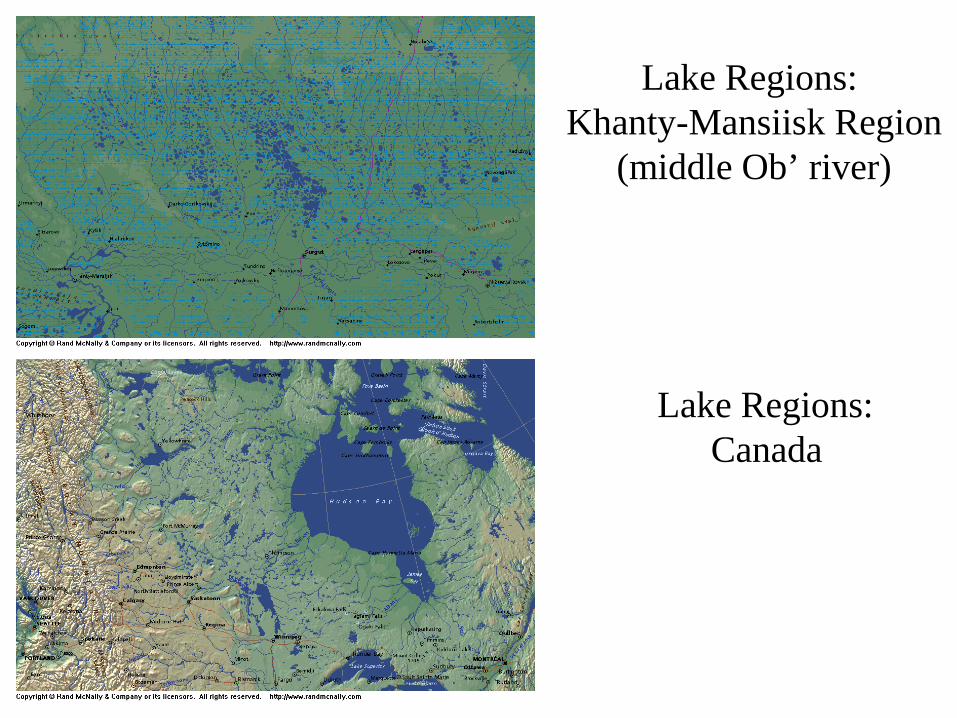
Lake Regions: Khanty-Mansiisk Region
(middle Ob’ river)
Lake Regions: Canada

Parameterisation of Lakes in NWP and Climate Models A Twofold Problem
(1a) The interaction of the atmosphere with the underlying surface is strongly dependent on the surface temperature and its time-rate-of-change. (Most) NWP systems assume that the water surface temperature can be kept constant over the forecast period. The assumption is doubtful for small-to-medium size relatively shallow lakes, where the diurnal variations of the surface temperature reach several degrees. A large number of such lakes will become resolved-scale features as the horizontal resolution is increased.
(1b) Apart from forecasting the lake surface temperature, its initialisation is also an issue.
(2) Lakes strongly modify the structure and the transport properties of the atmospheric surface layer. A major outstanding question is the parameterisation of the roughness of the water surface with respect to wind (e.g. limited fetch) and to scalar quantities.

Lake Parameterisation Schemes for NWP and Climate Models
Three-dimensional lake models
(or ocean models customised for lakes) provide detailed information about the lake temperature structure.
A very high computational cost limits their utility to only a few large lakes, such as Lake Victoria (Song et al. 2004), Laurentian Great Lakes (León et al. 2005), Great Slave Lake (León et al. 2007, Long et al. 2007) and Great Bear Lake (Long et al. 2007), and to research applications.
The use of three-dimensional lake models as lake parameterization schemes in NWP and other operational applications will most likely be impossible for some (perhaps many) years to come.

Lake Parameterisation Schemes for NWP and Climate Models (cont’d)
One-dimensional lake models (parameterisation schemes)
for NWP and climate modelling range from the simplest one-layer slab models to rather sophisticated turbulence closures.
• One-layer models
assume complete mixing down to the bottom (Ljungemyr et al. 1996), or to the bottom of a mixed layer of fixed depth (Goyette et al. 2000).
Neglect stratification (lake thermocline) ⇒ large errors in the surface temperature

Lake Parameterisation Schemes for NWP and Climate Models (cont’d)
• K-models with convective adjustment (Hostetler and Bartlein 1990, Hostetler 1991, Hostetler et al. 1993, Barrette and Laprise 2005). The Hostetler model enjoyed wide popularity in climate studies (e.g. Hostetler and Benson 1990, Hostetler 1991, Hostetler and Giorgi 1992, Bates et al. 1993, 1995, Hostetler et al. 1993, 1994, Bonan 1995, Small et al. 1999, Hostetler and Small 1999).
• Second-order turbulence closure models, e.g. models that carry transport equations for the TKE and its dissipation rate (Omstedt and Nyberg 1996, Omstedt 1999, Blenckner e tal. 2002, Stepanenko 2005, Stepanenko et al. 2006) or for the TKE only (Tsuang et al. 2001)
Multi-layer, finite-difference ⇒ expensive computationally

Lake Parameterisation Schemes for NWP and Climate Models (cont’d)
• A “conceptual” model of Croley (1989, 1992; Croley and Assel 1994)
is based on the heat budget arguments and a set of empirical rather ad hoc parameterisation rules (“wind aging function”) to account for vertical mixing. The model was used by Lofgren (1997) to assess the effect of North American Great Lakes on climate.
• A hybrid model of MacKay (2005)
is based on the solution of the non-steady heat transfer equation on a numerical grid in combination with the bulk treatment of the upper mixed layer (following Imberger 1985, and Spigel et al. 1986).
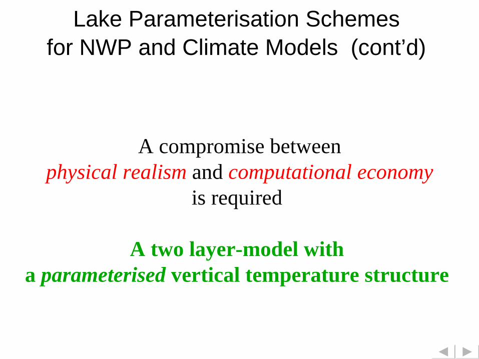
Lake Parameterisation Schemes for NWP and Climate Models (cont’d)
A compromise betweenphysical realism and computational economy
is required
A two layer-model with a parameterised vertical temperature structure

The Concept of Self-Similarity
of the Temperature Profile in the Thermocline
• Put forward by Kitaigorodskii and Miropolsky (1970) to describe the temperature structure of the oceanic seasonal thermocline. The essence of the concept is that the temperature profile in the thermocline can be fairly accurately parameterised through a “universal” function of dimensionless depth, using the temperature difference across the thermocline, ∆θ=θs(t)-θb(t), and its thickness, ∆h, as appropriate scales of temperature and depth:
.)(
)(),(
)(
),()(
th
thz
t
tzts
∆−==
∆− ςςϑθ
θθ

A Close Analogy to the Mixed-Layer Concept
• Using the mixed-layer temperature θ s(t) and its thickness h(t) as appropriate scales, the mixed-layer concept states that
,)(
),()(
),(
th
z
t
tzML
s
== ξξϑθ
θ
where the shape function υML is simply a constant equal to one.
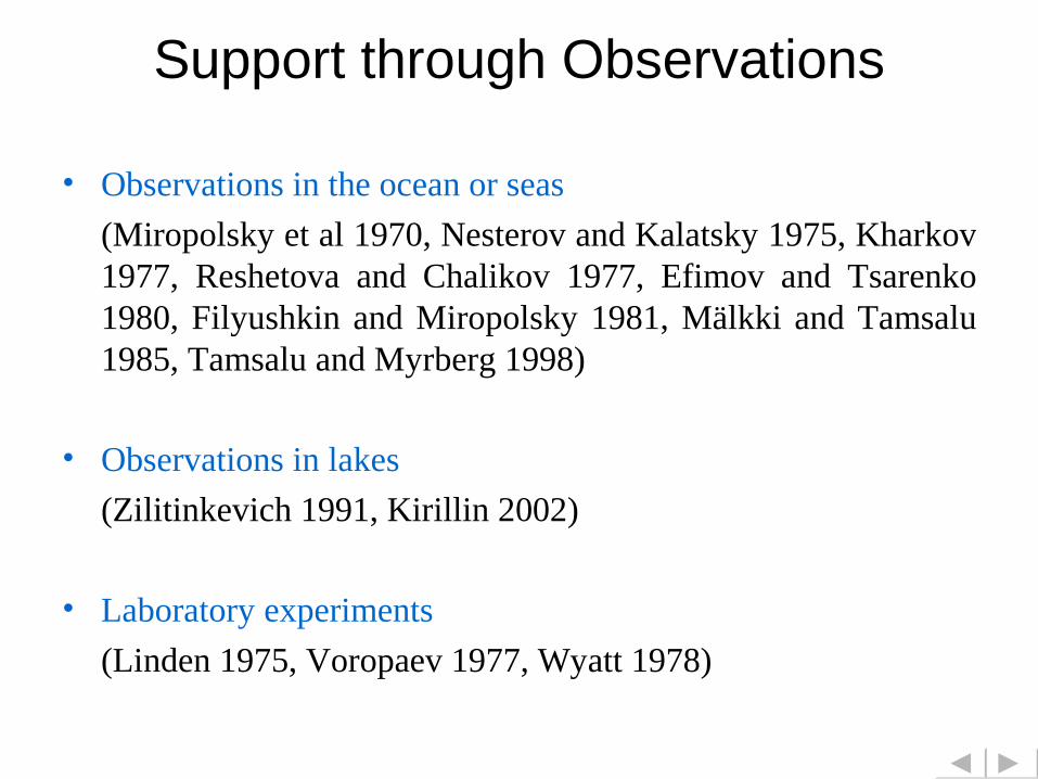
Support through Observations
• Observations in the ocean or seas
(Miropolsky et al 1970, Nesterov and Kalatsky 1975, Kharkov 1977, Reshetova and Chalikov 1977, Efimov and Tsarenko 1980, Filyushkin and Miropolsky 1981, Mälkki and Tamsalu 1985, Tamsalu and Myrberg 1998)
• Observations in lakes
(Zilitinkevich 1991, Kirillin 2002)
• Laboratory experiments
(Linden 1975, Voropaev 1977, Wyatt 1978)

Dimensionless temperature profile in the lake thermocline. Curves show a polynomial approximation (Kirillin 2002).

Dimensionless temperature profile in the lake thermocline. Points show data from measurements in Trout Bog (depth=7.7 m). Curves show a polynomial approximation (Kirillin 2002).

The Lake Model FLake (http://lakemodel.net)
• the surface temperature, • the bottom temperature, • the mixed-layer depth, • the shape factor with respect to the temperature profile in the thermocline, • the depth within bottom sediments penetrated by the thermal wave, and • the temperature at that depth.
The model is based on the idea of self-similarity (assumed shape) of the evolving temperature profile. That is, instead of solving partial differential equations (in z, t) for the temperature and turbulence quantities (e.g. TKE), the problem is reduced to solving ordinary differential equations for time-dependent parameters that specify the temperature profile. These are
In case of ice-covered lake, additional prognostic variables are • the ice depth, • the temperature at the ice upper surface, • the snow depth, and the temperature at the snow upper surface.
Important! The model does not require (re-)tuning.

Schematic Representation of the Temperature Profile
(a) The evolving temperature profile is characterised by a number of time-dependent parameters, namely, the temperature θ s(t) and the depth h(t) of the mixed layer, the bottom temperature θb(t), the shape factor CT(t) with respect to the temperature profile in the thermocline, the depth H(t) within bottom sediments penetrated by the thermal wave, and the temperature θH(t) at that depth.
θ
s(t)θ
b(t)
(a)
θL
θH
(t)
h(t)
D
L
H(t)
CT(t)

(b) In winter, four additional variables are computed, namely, the temperature θS(t) at the air-snow interface, the temperature θI(t) at the snow-ice interface, the snow thickness HS(t), and the ice thickness HI(t).
θs(t) θ
b(t)θ
I(t)θ
S(t)
(b)θ
L
θH
(t)
h(t)
D
L
H(t)
-HI(t)
-HI(t)-H
S(t)
Snow
Ice
Water
Sediment
CT(t)

Single-Column Tests
• Kossenblatter See, Germany (52 N, depth = 2 m)
• Lake Krasnoye, Russia (60 N, depth = 8 m)
• Lake Pääjärvi, Finland (61 N, depth = 15 m)
• Ryan Lake, USA (45 N, depth = 9 m)
Forcing in single-column mode Known from observations: • short-wave radiation flux, • long-wave radiation flux from the atmosphere.
Computed as part of the solution (depend on lake surface temperature): • long-wave downward radiation flux from the surface, • fluxes of momentum and of sensible and latent heat, • for ice-covered lakes, surface albedo.
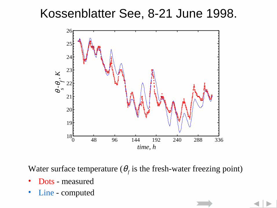
Kossenblatter See, 8-21 June 1998.
Water surface temperature (θ f is the fresh-water freezing point)
• Dots - measured • Line - computed
0 48 96 144 192 240 288 33618
19
20
21
22
23
24
25
26
time, h
θs- θ
f , K

Kossenblatter See, 8-21 June 1998.
Friction velocity in the surface air layer • Symbols - measured • Line - computed
216 240 264 288 3120
0.1
0.2
0.3
0.4
0.5
time, h
u* ,
m⋅ s
-1

Kossenblatter See, 8-21 June 1998.
• Sensible heat flux Qse
• Latent heat flux Qla
• Symbols – measured
• Lines– computed 216 240 264 288 312
-80
-60
-40
-20
0
20
time, h
Qse
, W
⋅ m-2
216 240 264 288 312-300
-250
-200
-150
-100
-50
0
time, h
Qla
, W
⋅ m-2

Lake Krasnoye, 1 May - 31 October 1970.
Water surface temperature θ s (θf is the fresh-water freezing point)
Dots – measured, line - computed
120 150 180 210 240 270 3000
5
10
15
20
25
time, day
θs- θ
f , K
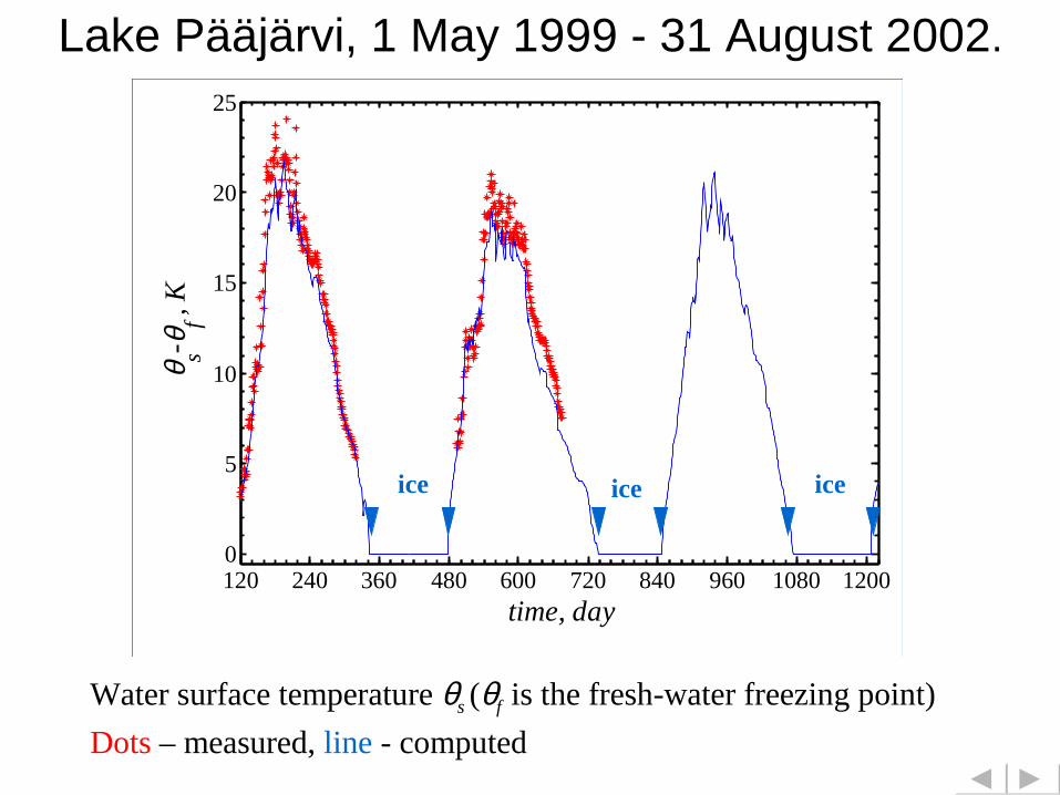
Lake Pääjärvi, 1 May 1999 - 31 August 2002.
Water surface temperature θs (θf is the fresh-water freezing point)
Dots – measured, line - computed
120 240 360 480 600 720 840 960 1080 12000
5
10
15
20
25
time, day
θs- θ
f , K
ice ice ice

Lake Ryan, November 1989 – November 1990.
Surface temperature, mean temperature of the water column, bottom temperature
Dotted – measured, solid – modelled
-30 0 60 120 180 240 3000
5
10
15
20
25
30
35
time, day
θ- θ
f , K
Ice
? (sensor malfunction)

Lake Ryan, April – November 1990.
Mean temperature of the water column
Measured vs. modelled
90 120 150 180 210 240 270 3000
5
10
15
20
time, day
θm
- θf ,
K

Lake Ryan, December 1989.
• Solid - modelled ice surface temperature • Dotted - temperature measured with the uppermost sensor
-30 -20 -10 0
-25
-20
-15
-10
-5
0
time, day
θi- θ
f , K
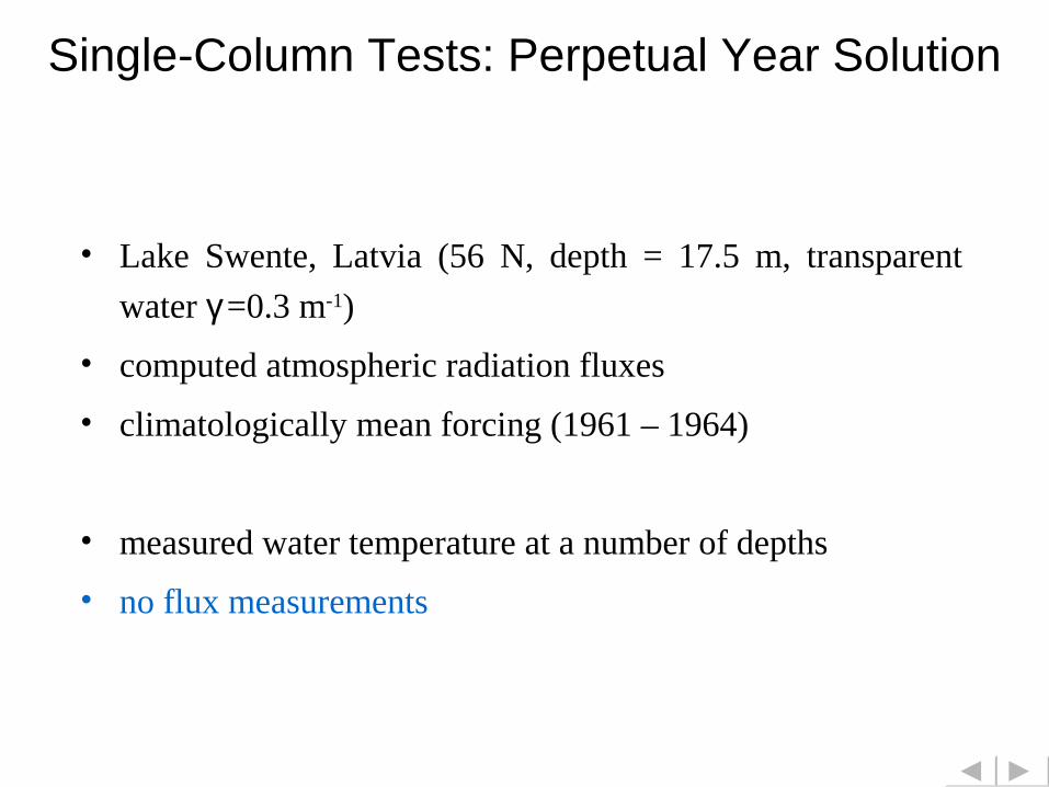
Single-Column Tests: Perpetual Year Solution
• Lake Swente, Latvia (56 N, depth = 17.5 m, transparent
water γ =0.3 m-1)
• computed atmospheric radiation fluxes
• climatologically mean forcing (1961 – 1964)
• measured water temperature at a number of depths
• no flux measurements

Lake Swente, Perpetual Year.
Surface temperature, mean temperature of the water column, bottom temperature
Symbols – measured, lines – modelled
0 60 120 180 240 300 360
0
5
10
15
20
time, day
θ- θ
f , K
Ice

FLake in NWP and Climate Models:
External Parameters
• geographical latitude (easy)
• lake fraction of the NWP model grid-box (not so easy)
• lake depth (not easy at all, e.g. for the lack of data)
• typical wind fetch
• optical characteristics of lake water (extinction coefficients with
respect to solar radiation)
• depth of the thermally active layer of bottom sediments, temperature
at that depth (cf. soil model parameters)
Default values of the last four parameters can be used.
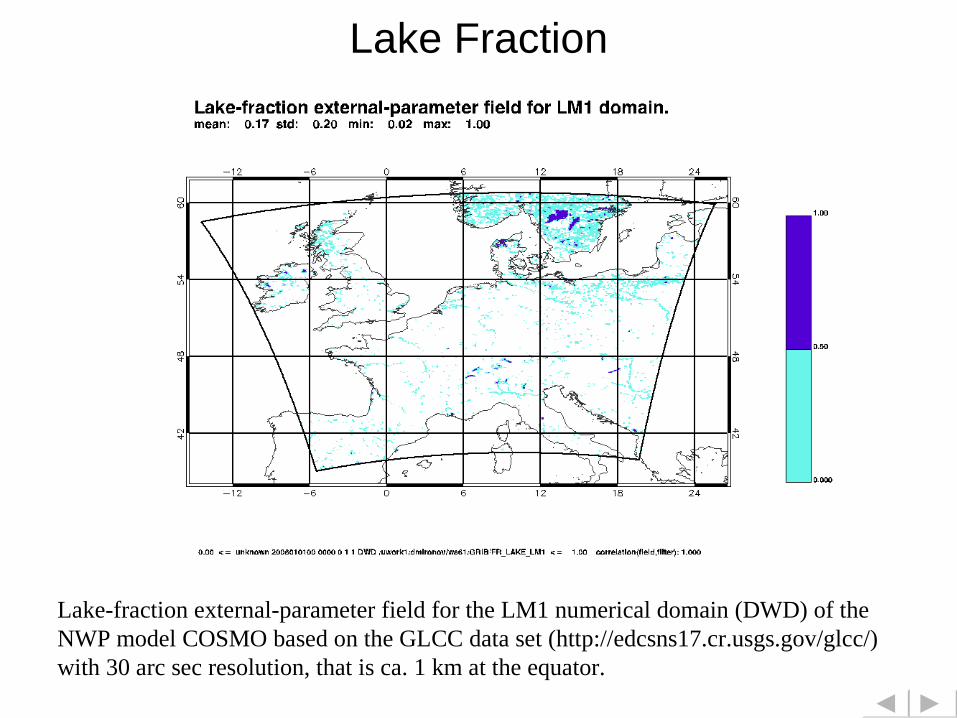
Lake Fraction
Lake-fraction external-parameter field for the LM1 numerical domain (DWD) of the NWP model COSMO based on the GLCC data set (http://edcsns17.cr.usgs.gov/glcc/) with 30 arc sec resolution, that is ca. 1 km at the equator.

Lake Depth
Lake depths for the LM1 numerical domain of the NWP model COSMO. The field is developed (Natalia Schneider) using various data sets. Each lake is characterised by its mean depth.

FLake in COSMO: Parallel Experiment
• No tile approach: lakes are the COSMO-model grid-boxes with
FR_LAKE>0.5, otherwise land or sea water
• 2D fields of lake fraction and of lake depth (limited by 50 m), default values
of other lake-specific parameters
• COSMO-model parallel experiment (including the entire data assimilation
cycle) over 1 year, 1 January through 31 December 2006
• “Artificial” initial conditions, where the lake surface temperature is equal to
the COSMO-model SST from the assimilation
• Turbulent fluxes are computed with the COSMO-model surface-layer scheme
(Raschendorfer 2001); optionally, the new surface-layer scheme (Mironov et
al. 2003, http://lakemodel.net) can be used
• The effect of snow is accounted for implicitly through the surface albedo

FLake in COSMO: Results from Parallel Experiment 56321 January – 31 December 2006
Lake Hjälmaren, Sweden (mean depth = 6.1 m)• Black – lake surface temperature from the COSMO-LM SST analysis • Green – lake surface temperature computed with FLake

FLake in COSMO: Results from Parallel Experiment 56321 January – 31 December 2006
Lake Hjälmaren, Sweden (mean depth = 6.1 m)
Ice thickness (left) and ice surface temperature (right) computed with COSMO-LM-FLake

FLake in COSMO: Results from Parallel Experiment 56321 January – 31 December 2006
Lake Balaton, Hungary (mean depth = 3.3 m)• Black – lake surface temperature from the COSMO-LM SST analysis • Green – lake surface temperature computed with FLake

FLake in COSMO: Results from Parallel Experiment 56321 January – 31 December 2006
Lake Balaton, Hungary (mean depth = 3.3 m)
Ice thickness (left) and ice surface temperature (right) computed with COSMO-LM-FLake

FLake in COSMO: Results from Parallel Experiment 56321 January – 31 December 2006
Neusiedlersee, Austria-Hungary (mean depth = 0.8 m)• Black – lake surface temperature from the COSMO-LM SST analysis • Green – lake surface temperature computed with FLake

FLake in COSMO: Results from Parallel Experiment 56321 January – 31 December 2006
Lake Vänern, Sweden (mean depth = 27 m)• Black – lake surface temperature from the COSMO-LM SST analysis • Green – lake surface temperature computed with FLake

FLake in COSMO: Results from Parallel Experiment 56321 January – 31 December 2006
Lago Maggiore, Italy-Switzerland (mean depth = 177 m)• Black – lake surface temperature from the COSMO-LM SST analysis • Green – lake surface temperature computed with FLake

FLake in COSMO: Results from Parallel Experiment 56321 January – 31 December 2006
Lough Neagth, UK (mean depth = 8.9 m)• Black – lake surface temperature from the COSMO-LM SST analysis • Green – lake surface temperature computed with FLake

Conclusions
• The lake model FLake shows a satisfactory performance in single-column experiments
• FLake is implemented into the limited-area NWP model COSMO, results from test runs look promising
Outlook • A comprehensive lake-depth data set (European, eventually global) • The cold start spin-up problem • Three-layer extension (deep lakes)
FLake Page http://lakemodel.net (also http://nwpi.krc.karelia.ru/flake)

Thanks for your attention!
and
Welcome to the FLake Club!
Acknowledgements: Michael Buchhold, Günther Doms, Thomas Hanisch, Peter Meyring, Van Tan Nguyen, Ulrich Schättler, Christoph Schraff (DWD), Anders Ullerstig (SMHI, Norrköping), Burkhardt Rockel (GKSS, Geesthacht), Viktor Stepanenko (Moscow State University), Emanuel Dutra (University of Lisbon).
The work was partially supported by the EU Commissions, Projects INTAS-01-2132 and INTAS-05-1000007-431.
Empirical data from Lake Pääjärvi are made available through the collaboration with the Division of Geophysics of the University of Helsinki that is supported by the Academy of Finland (project “Ice Cover in Lakes and Coastal Seas”) and by the Vilho, Yrjö and Kalle Väisälä Foundation of the Academy of Sciences and Letters, Finland (project “Modelling of Boreal Lakes”).

FLake in NWP Models: the Spin-Up Problem
• Lakes have a long memory: wrong initial conditions result in wrong heat content and in wrong water-surface temperature until the memory is faded. This may last up to a year.
• Observations offer water-surface temperature, whereas the vertical temperature structure (mean temperature of the water column, bottom temperature, mixed-layer depth) is unknown.
A Way Out • generate forcing for the entire annual cycle (using observational
data, or an NPW model output) • set-up single-column runs (computationally cheap!) with
arbitrary (!) initial conditions • repeat a year-long integration cyclically until a perpetual-year
periodic solution is obtained; such solution corresponds the climatological-mean state of a given lake
• take initial conditions for the cold start from that perpetual-year solution

Stuff Unused

FLake Applications
• Lake parameterisation scheme for NWP and climate models
(computationally efficient, can be used to treat a large number of lakes)
• Single-column lake model in a stand-alone mode (assessment of
response of lakes to climate variability, estimation of evaporation from
the water surface, aid in design of ponds and reservoirs, etc., a cost-
effective decision-making tool)
• Physical module in models of lake ecosystems (a sophisticated physical
module is not required because of large uncertainties in chemistry and
biology)
• Educational tool (simple but incorporates much of the essential
physics)