Flavours of Physics Challenge: Physics Prize

Transfer Learning approach

1

Heavy Flavour Data Mining workshop

18 February 2016, Zurich

Alexander Rakhlin rakhlin@gmx.net

Abstract

When modeling a classifier on simulated data, it is possible to reach a high

performance by picking features that are not perfectly modeled in the

simulation. To avoid this problem in Kaggle’s "Flavours of Physics: Finding 𝜏-→𝜇-𝜇-𝜇+ " competition a proxy channel with similar topology and well-studied

characteristics was introduced.

This proxy channel was intended for validation of classifier trained on another

channel of interest. We show that such validation scheme is questionable from

a point of view of statistical inference as it violates fundamental assumption in

Machine Learning that training and test data follow the same probability

distribution.

Abstract 2

Proposed solution:

Transfer Learning

We relate the problem to known paradigm in Machine Learning – Transfer

Learning between different underlying distributions.

We propose a solution that brings the problem to transductive transfer learning

(TTL) and simple covariate shift, a primary assumption in domain adaptation

framework.

Finally, we present transfer learning model (one of a few) that finished the

competition on the 5 place.

Abstract 3

1. INTRODUCTION

4

Description

Like 2014’ Higgs Boson Kaggle Challenge, this competition dealt with the

physics at the Large Hadron Collider.

However, the Higgs Boson was already known to exist. The goal of 2015’

challenge was to design a classifier capable to discriminate a phenomenon that

is not already known to exist – charged lepton flavour violation – thereby

helping to establish "new physics" (from the competition description)

1. Introduction

5

The data

For training the classifier participants were given ~800,000 signal and

background samples of labeled data from 𝜏-→𝜇-𝜇-𝜇+ channel.

Background events come from real data, whereas signal events come from

Monte-Carlo simulation. Hereinafter:

• 𝜏-→𝜇-𝜇-𝜇+ channel shall be referred to as 𝜏 channel

• its background data samples – as 𝑋𝑑𝑎𝑡𝑎𝜏

• its Monte-Carlo simulated signal data samples – as 𝑋𝑀𝐶𝜏

• The signal being “1” for events where the decay did occur, “0” for

background events where it did not.

1. Introduction 6

Control channel

Since the classifier was trained on simulated data for the signal and on real

data for the background, it was possible to reach a high performance by

picking features that are not perfectly modeled in the simulation.

To address this problem a Control channel with known characteristics was

introduced, and classifier was required not to have large discrepancy when

applied to 𝜏 and control channel. Kolmogorov–Smirnov test (Agreement test)

was used to make sure that classifier performance does not vary significantly

between the channels.

1. Introduction

7

Control channel (continued)

Control channel Ds+→(→𝜇-𝜇+)+ has a similar topology as the 𝜏 channel, and is a

much more well-known, well-observed behavior, as it happens more frequently.

Just like for 𝜏 channel participants were provided with both Monte-Carlo

simulated and real data for Ds+→(→𝜇-𝜇+)+ decay to which the classifier can be

verified. In addition, sPlot weights were assigned to real data. Higher weight

means an event is likely to be signal, lower weight means it’s likely to be

background. Real data is a mix of real decay and background events with large

prevalence of background. Hereinafter:

• Ds+→(→𝜇-𝜇+)+ channel shall be referred to as 𝐷𝑠 −channel

• its real data samples (mainly background) – as 𝑋𝑑𝑎𝑡𝑎𝐷𝑠

• its Monte-Carlo simulated signal samples – as 𝑋𝑀𝐶𝐷𝑠

1. Introduction

8

Evaluation

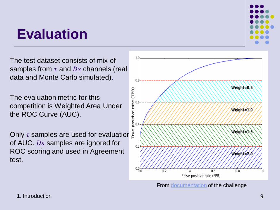
The test dataset consists of mix of

samples from 𝜏 and 𝐷𝑠 channels (real

data and Monte Carlo simulated).

The evaluation metric for this

competition is Weighted Area Under

the ROC Curve (AUC).

Only 𝜏 samples are used for evaluation

of AUC. 𝐷𝑠 samples are ignored for

ROC scoring and used in Agreement

test.

1. Introduction 9

From documentation of the challenge

No training on 𝑫𝒔 channel

allowed

𝐷𝑠 channel was not intended for training, its purpose was validation of

already trained classifier in KS-test.

1. Introduction

10

This requirement became the main challenge of “Flavours of Physics: Finding 𝜏-→𝜇-𝜇-𝜇+“, and constitutes central point of this presentation.

The problem: validation on 𝑫𝒔

channel is questionable

In the following we demonstrate that 𝜏 and 𝐷𝑠 channels have

significantly different probability distributions.

On the other hand, Machine Learning theory shall remind us why testing

on data that has different probability distribution than data where the

model was created violates …

1. Introduction

11

This assumption is the cornerstone of statistical learning and, in

general, of inference.

… the assumption of a single underlying generative process between the train set and the test set.

Our plan

o The following section is dedicated to foundations of Machine Learning

theory. We demonstrate there that 𝜏 and 𝐷𝑠 channels have different

underlying probability distributions and argue why it is bad.

o In “Transfer learning” section we propose a framework for learning from

different distributions.

o “Implementation” section discusses solution presented for this competition

and sets some guidelines for further development.

o “Kolmogorov–Smirnov test” section is optional but provides some

interesting insight.

1. Introduction

12

2. BRIEF REVIEW OF MACHINE

LEARNING FOUNDATIONS

Let us briefly recall the fundamentals of Machine Learning theory.

13

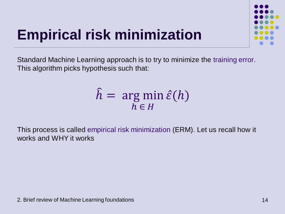
Empirical risk minimization

Standard Machine Learning approach is to try to minimize the training error.

This algorithm picks hypothesis such that:

ℎ = arg minℎ ∈ 𝐻

𝜀 (ℎ)

This process is called empirical risk minimization (ERM). Let us recall how it

works and WHY it works

2. Brief review of Machine Learning foundations 14

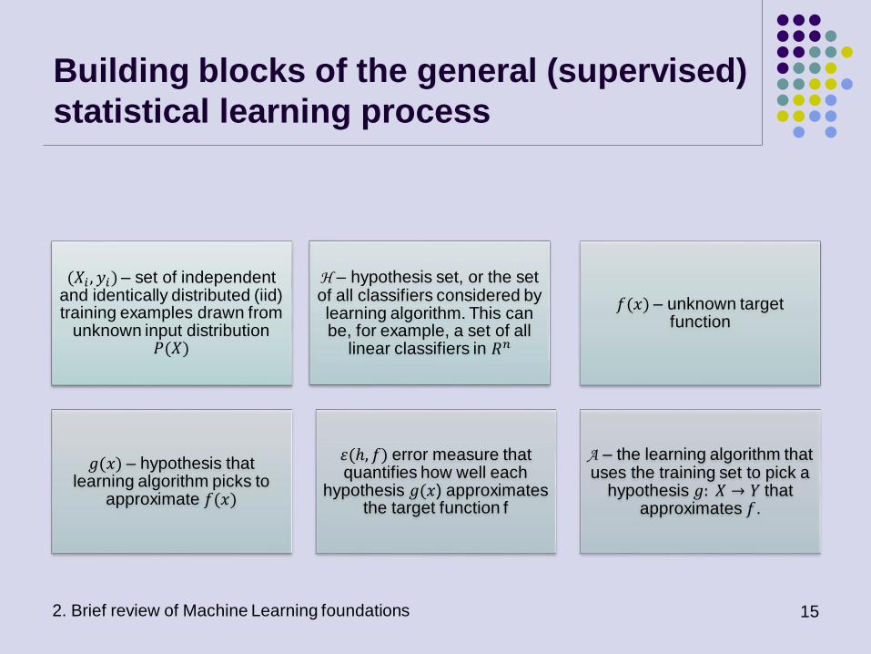
Building blocks of the general (supervised)

statistical learning process

2. Brief review of Machine Learning foundations 15

(𝑋𝑖 , 𝑦𝑖) – set of independent and identically distributed (iid) training examples drawn from

unknown input distribution 𝑃(𝑋)

H – hypothesis set, or the set of all classifiers considered by learning algorithm. This can be, for example, a set of all

linear classifiers in 𝑅𝑛

𝑓(𝑥) – unknown target function

𝑔(𝑥) – hypothesis that learning algorithm picks to

approximate 𝑓(𝑥)

𝜀(ℎ, 𝑓) error measure that quantifies how well each

hypothesis 𝑔(𝑥) approximates the target function f

A – the learning algorithm that uses the training set to pick a

hypothesis 𝑔: 𝑋 → 𝑌 that approximates 𝑓.

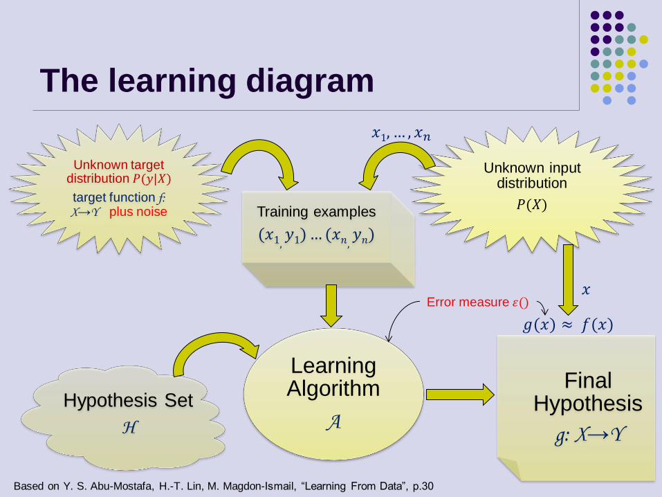
The learning diagram

Unknown input distribution

𝑃(𝑋)

Learning Algorithm

A

Unknown target distribution 𝑃(𝑦|𝑋)

target function f: X→Y plus noise

Final Hypothesis

g: X→Y

Training examples

(𝑥1,𝑦1)… (𝑥𝑛,

𝑦𝑛)

Hypothesis Set

H

𝑥

𝑥1, … , 𝑥𝑛

Error measure 𝜀()

𝑔(𝑥) ≈ 𝑓(𝑥)

Based on Y. S. Abu-Mostafa, H.-T. Lin, M. Magdon-Ismail, “Learning From Data”, p.30

Generalization

Generalization is ability to perform well on unseen data, is what

Machine Learning is ultimately about.

Why should doing well on the training set tell us anything about

generalization error? Can we prove that learning algorithms will work

well?

2. Brief review of Machine Learning foundations 17

Most learning algorithms fit their models to the training set, but what we really

care about is generalization error, or expected error on unseen examples.

Hoeffding’s inequality

2. Brief review of Machine Learning foundations 18

It is possible to prove this most important result in learning theory using just two

lemmas [2], [3]:

the union bound

Hoeffding’s inequality (Chernoff bound) which provides an upper bound on

the probability that the sum of independent and identically distributed (iid)

random variables deviates from its expected value.

𝑃(|𝜀 ℎ𝑖 − 𝜀 ℎ𝑖 | > 𝛾) ≤ 2𝑘𝑒−2𝛾2𝑚

This means that for all ℎ𝑖 ∈ 𝐻 (*) generalization error 𝜀 will be close to training

error 𝜀 with “high” probability, assuming 𝑚 - the number of training examples -

is “large”.

* for simplicity we assume 𝐻 is discrete hypothesis set consisting of 𝑘 hypotheses, but in learning

theory this result extrapolates to infinite 𝐻 [2], [3]

iid assumption

2. Brief review of Machine Learning foundations 19

Note that Hoeffding’s inequality does not make any prior assumption about the

data distribution. Its only assumption is that the training and testing data are

independent and identically distributed (iid) random variables drawn from the same distribution D

The assumption of training and testing on the same distribution is the most important in a set of

assumptions under which numerous results on learning theory were proved.

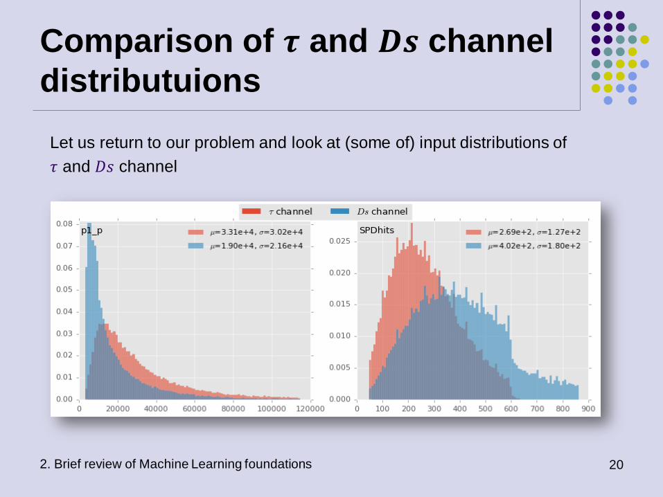
Comparison of 𝝉 and 𝑫𝒔 channel

distributuions

2. Brief review of Machine Learning foundations 20

Let us return to our problem and look at (some of) input distributions of

𝜏 and 𝐷𝑠 channel

21 2. Brief review of Machine Learning foundations

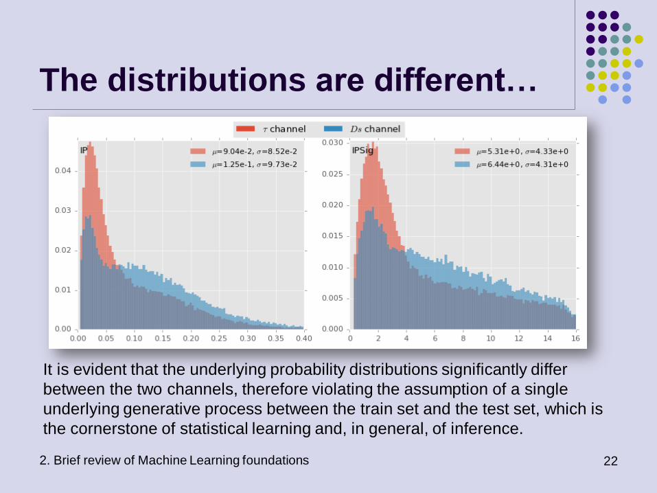
The distributions are different…

2. Brief review of Machine Learning foundations 22

It is evident that the underlying probability distributions significantly differ

between the two channels, therefore violating the assumption of a single

underlying generative process between the train set and the test set, which is

the cornerstone of statistical learning and, in general, of inference.

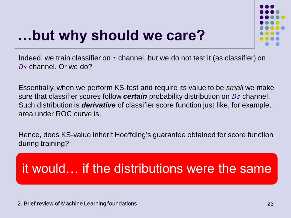
…but why should we care?

2. Brief review of Machine Learning foundations 23

Indeed, we train classifier on 𝜏 channel, but we do not test it (as classifier) on

𝐷𝑠 channel. Or we do?

Essentially, when we perform KS-test and require its value to be small we make

sure that classifier scores follow certain probability distribution on 𝐷𝑠 channel.

Such distribution is derivative of classifier score function just like, for example,

area under ROC curve is.

Hence, does KS-value inherit Hoeffding’s guarantee obtained for score function

during training?

it would… if the distributions were the same

What does it mean for us?

2. Brief review of Machine Learning foundations 24

Practically this means that Kolmogorov–Smirnov test provides no guarantee [in

statistical sense] for KS value on 𝐷𝑠 channel where a model was not trained. At

the best, low KS value can be achieved by chance, and there is no guarantee it

remains small with some other 𝐷𝑠 data.

To draw conclusions from different distribution that did not participate in inference is generally useless - as long

as we hold on Machine Learning paradigm.

3. KOLMOGOROV–SMIRNOV

TEST

Before we propose a solution to the problem of different

distributions let us review nuances of Kolmogorov–Smirnov test

that played interesting role in this competition.

25

Kolmogorov–Smirnov test

3. Kolmogorov–Smirnov test 26

One of the competition requirements for the classifier is small discrepancy

when applied to data and to simulation. Kolmogorov–Smirnov test [9,

Agreement test] evaluates distance between the empirical distributions of the

classifier scores on 𝐷𝑠 channel:

𝐾𝑆 = sup |𝐹𝑀𝐶 − 𝐹𝑑𝑎𝑡𝑎∗ |

where 𝐹𝑀𝐶 and 𝐹𝑑𝑎𝑡𝑎 are cumulative distribution functions (CDF) of the

classifier scores 𝑠(𝑋) for 𝑋𝑑𝑎𝑡𝑎𝐷𝑠 (real, mainly background) and 𝑋𝑀𝐶

𝐷𝑠 (simulated,

signal). Asterisk in 𝐹𝑑𝑎𝑡𝑎∗ stands for sPlot adjusted distribution 𝐹𝑑𝑎𝑡𝑎 (see next

slide)

Score distribution agreement on

𝑫𝒔 channel

3. Kolmogorov–Smirnov test 27

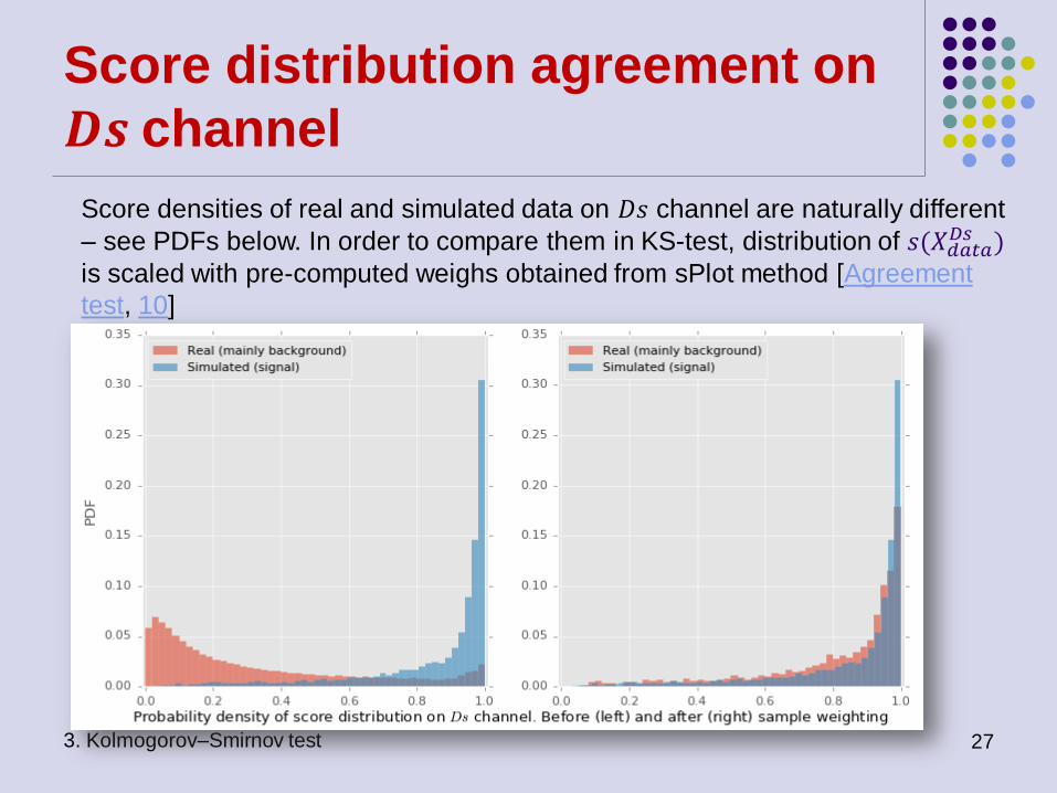
Score densities of real and simulated data on 𝐷𝑠 channel are naturally different

– see PDFs below. In order to compare them in KS-test, distribution of 𝑠(𝑋𝑑𝑎𝑡𝑎𝐷𝑠 )

is scaled with pre-computed weighs obtained from sPlot method [Agreement

test, 10]

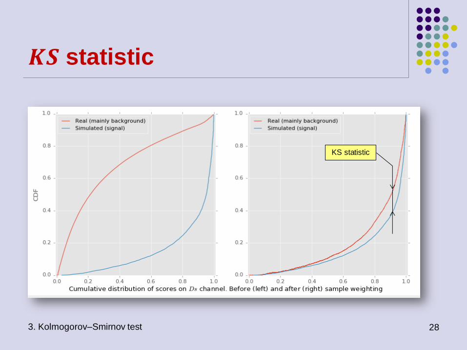
𝑲𝑺 statistic

3. Kolmogorov–Smirnov test 28

KS statistic

A degenerate case

3. Kolmogorov–Smirnov test 30

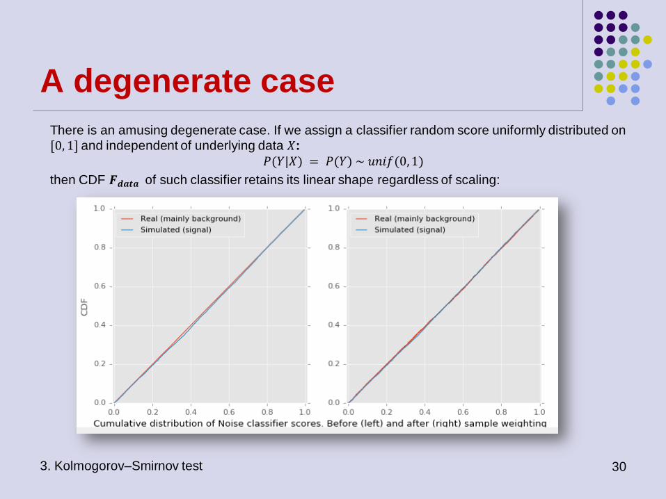
There is an amusing degenerate case. If we assign a classifier random score uniformly distributed on

[0, 1] and independent of underlying data 𝑋:

𝑃(𝑌|𝑋) = 𝑃(𝑌) ~ 𝑢𝑛𝑖𝑓(0,1)

then CDF 𝑭𝒅𝒂𝒕𝒂 of such classifier retains its linear shape regardless of scaling:

A degenerate case (continued)

3. Kolmogorov–Smirnov test 31

Not affected by sample weighting, such “classifier” can easily pass KS-test on 𝐷𝑠 channel. To

demonstrate this, author of this presentation has implemented a simple model, combination of “strong”

classifier and random noise. This model works as follows:

1. “Real” or “strong” classifier assigns scores to all test samples.

2. Samples with scores below certain (rather high) threshold 𝑇 < 1 change their score to random

noise ~ 𝑢𝑛𝑖𝑓(0, 𝑇)

3. Due to imperfect MC-simulation on 𝝉 channen and different 𝝉 and 𝑫𝒔 distributions most

𝑋𝑀𝐶𝜏 samples get high scores > 𝑇, while most 𝑋𝑑𝑎𝑡𝑎

𝜏 , 𝑋𝑀𝐶𝐷𝑠 , 𝑋𝑑𝑎𝑡𝑎

𝐷𝑠 get random scores < 𝑇 This

randomness is enough for 𝑋𝑀𝐶𝐷𝑠 , 𝑋𝑑𝑎𝑡𝑎

𝐷𝑠 samples to satisfy KS test on 𝑫𝒔 channel.

To summarize, different samples get scores from different classifiers. 𝑫𝒔 channel is de facto controlled

by “random” classifier, 𝝉 channel – by “strong” classifier. Although 𝑋𝑀𝐶𝐷𝑠 , 𝑋𝑑𝑎𝑡𝑎

𝐷𝑠 pass KS test on 𝑫𝒔

channel, this test has nothing to do with 𝝉 channel and can not assure quality of 𝑋𝑀𝐶𝜏 . Please see this

discussion for details.

Of course, this is very artificial example, but it shows practical evidence against

testing on different distribution.

4. SOLUTION: TRANSFER

LEARNING

32

Preamble

4. Solution: transfer learning 33

The idea of attesting model on control channel is certainly reasonable and can

be implemented in theoretically sound way. In Machine Learning the problem of

different data sets is well known, and solution is called Transfer learning. It

aims at transferring knowledge from a model created on the train data set to

the test data set, assuming they differ in some aspects, e.g. in distribution.

Transfer learning applications

4. Solution: transfer learning 34

The need for data set adaptation arises in many Machine Learning

applications. For example, spam filters can be trained on some public

collection of spam, but when applied to an individual mail box may require

personalization, i.e. adaptation to specific distribution of emails.

Medicine is another field for transfer learning, as models trained on general

population do not fit well individual subjects. The solution is to transfer such

models to individuals with adaptation. Brain-computer interface (BCI) is

another example of successful application of transfer learning [4]

One common characteristic of these problems is that target

domain of interest either has different distribution and little or no

labeled data, or is unavailable at training time at all.

Example

4. Solution: transfer learning 35

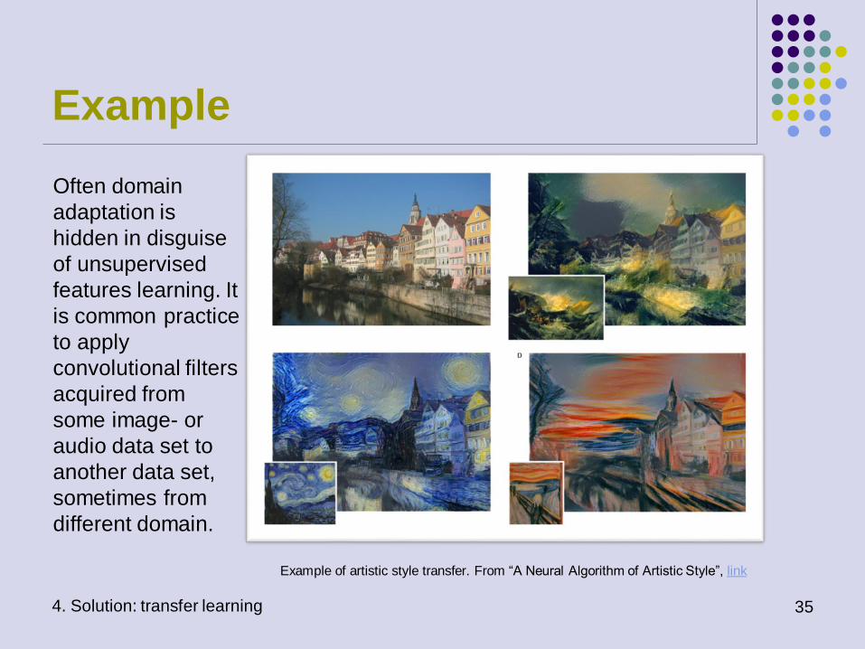
Often domain

adaptation is

hidden in disguise

of unsupervised

features learning. It

is common practice

to apply

convolutional filters

acquired from

some image- or

audio data set to

another data set,

sometimes from

different domain.

Example of artistic style transfer. From “A Neural Algorithm of Artistic Style”, link

Setting our goals

4. Solution: transfer learning 36

Our goal is formulated as follows: we have data from two channels of similar

topology and different distribution. The first channel we consider “reliable” (well-

studied behavior, reliable data), we use it as Source for transfer learning. The

second – “experimental” (less reliable data), we call it Target. We train logistic

regression on Source channel and transfer it to Target channel. In addition, we

may require our classifier to satisfy some other criteria, like KS and CvM tests.

Only physicists can decide which of the two channels – 𝜏 and 𝐷𝑠 – is

the Source, and which is the Target. In this section we depart from

original competition defaults and assume the reverse order: 𝐷𝑠 is the

Source (as more reliable data) and 𝜏 is the Target. It looks more natural

to us, but we can be wrong in this assumption. “Implementation”

section follows the original order set by the competition design, just like

our real solution.

Formal definitions

4. Solution: transfer learning 37

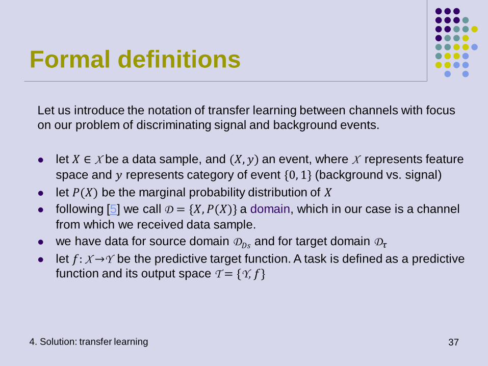
Let us introduce the notation of transfer learning between channels with focus

on our problem of discriminating signal and background events.

let 𝑋 ∈ X be a data sample, and (𝑋, 𝑦) an event, where X represents feature

space and 𝑦 represents category of event {0, 1} (background vs. signal)

let 𝑃(𝑋) be the marginal probability distribution of 𝑋

following [5] we call D = {𝑋, 𝑃(𝑋)} a domain, which in our case is a channel

from which we received data sample.

we have data for source domain D𝐷𝑠 and for target domain D𝜏

let 𝑓: X →Y be the predictive target function. A task is defined as a predictive

function and its output space T = {Y, 𝑓}

Transductive Transfer Learning

4. Solution: transfer learning 38

As stated in [5], “transfer learning aims to help improve the learning of the target predictive function 𝑓T in DT using the knowledge in DS and TS where, in

general, DS≠DT and TS≠TT”.

Our problem has two different but related domains D𝐷𝑠 and D𝜏, and the tasks

are the same in both domains: discriminating signal from background events,

T𝐷𝑠 = T𝜏 = T. Moreover, the source domain D𝐷𝑠 has labeled data set, and the

target domain has unlabeled data D𝜏 (notice the difference with original

competition formulation). This specific setting of the transfer learning problem is

called transductive transfer learning (TTL) [4]

Covariate Shift

4. Solution: transfer learning 39

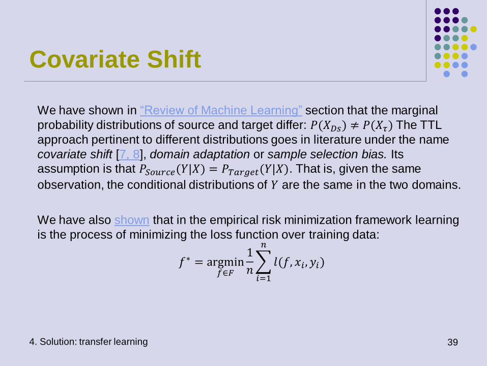
We have shown in “Review of Machine Learning” section that the marginal

probability distributions of source and target differ: 𝑃(𝑋𝐷𝑠) ≠ 𝑃(𝑋𝜏) The TTL

approach pertinent to different distributions goes in literature under the name

covariate shift [7, 8], domain adaptation or sample selection bias. Its

assumption is that 𝑃𝑆𝑜𝑢𝑟𝑐𝑒(𝑌|𝑋) = 𝑃𝑇𝑎𝑟𝑔𝑒𝑡(𝑌|𝑋). That is, given the same

observation, the conditional distributions of 𝑌 are the same in the two domains.

We have also shown that in the empirical risk minimization framework learning

is the process of minimizing the loss function over training data:

𝑓∗ = argmin𝑓∈𝐹

1

𝑛 𝑙(𝑓, 𝑥𝑖, 𝑦𝑖)

𝑛

𝑖=1

TTL framework

4. Solution: transfer learning 40

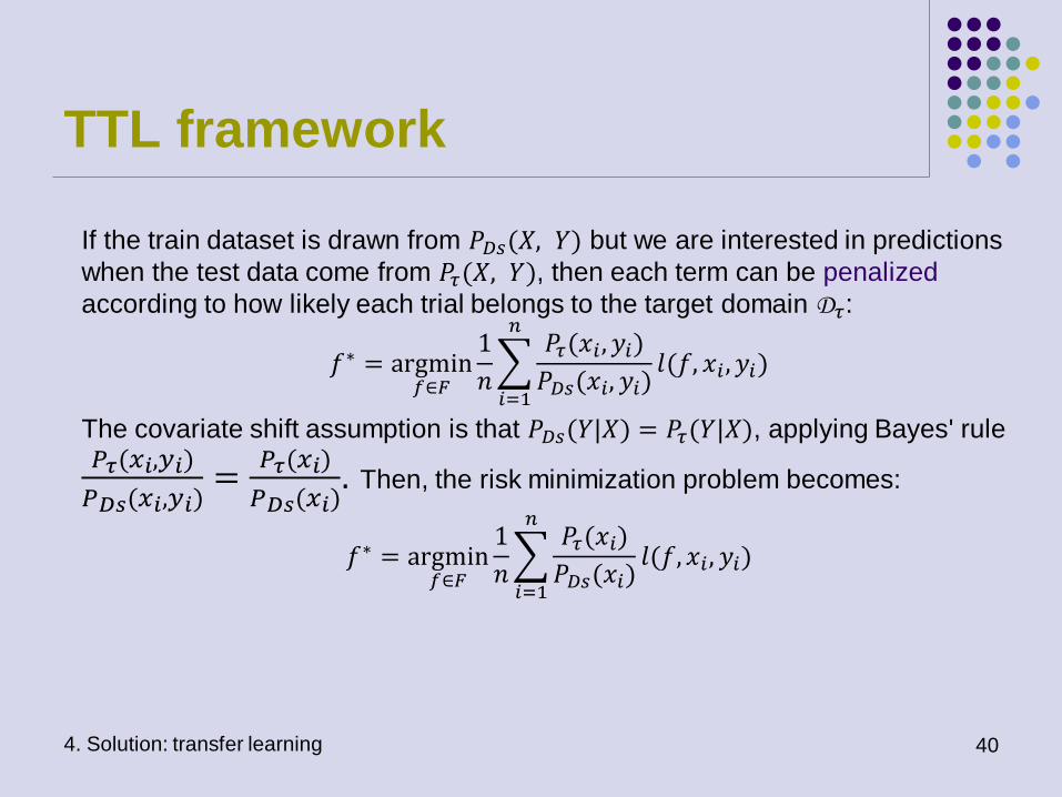
If the train dataset is drawn from 𝑃𝐷𝑠(𝑋, 𝑌) but we are interested in predictions

when the test data come from 𝑃𝜏(𝑋, 𝑌), then each term can be penalized

according to how likely each trial belongs to the target domain D𝜏:

𝑓∗ = argmin𝑓∈𝐹

1

𝑛

𝑃𝜏(𝑥𝑖, 𝑦𝑖)

𝑃𝐷𝑠(𝑥𝑖, 𝑦𝑖)𝑙(𝑓, 𝑥𝑖, 𝑦𝑖)

𝑛

𝑖=1

The covariate shift assumption is that 𝑃𝐷𝑠(𝑌|𝑋) = 𝑃𝜏(𝑌|𝑋), applying Bayes' rule 𝑃𝜏(𝑥𝑖,𝑦𝑖)

𝑃𝐷𝑠(𝑥𝑖,𝑦𝑖)=

𝑃𝜏(𝑥𝑖)

𝑃𝐷𝑠(𝑥𝑖). Then, the risk minimization problem becomes:

𝑓∗ = argmin𝑓∈𝐹

1

𝑛

𝑃𝜏(𝑥𝑖)

𝑃𝐷𝑠(𝑥𝑖)𝑙(𝑓, 𝑥𝑖, 𝑦𝑖)

𝑛

𝑖=1

Covariate shift: Toy example

41

S

S

S

S

S

S

S

S

S

S

S

S

S

S

S

S

S

S

S

S

S

S

S

S

S

S

S

S

S

S

S

S

S

S

S

S

S

S

S

S

S

S

S

S

S

S

S

S

S

S

S

S

S

S

S

S

S

S

S

S

S

S

S

S

S

S

S

S

S

S

S

S

S

S

S

S

S

S

S

S

S

S

S

S

S

S

S

S

S

S

S

S

S

S

S

S

S

S S S

S

S

S

S

S

S

S

S

S

S

S

S

S

S

S

S

S

S

S

S

S

S

S

S

S

S

S

S

S

S

S

S S

S

S

S

S

S

S

S

S

S

S

S

S

S

S

S

S

S

S

S

S

S

S

S

S

S

S

S

S

S

S

S

S

S

S

S

S

S

S

S

S

S

S

S

S

S

S

S

S

S

S

S

S

S

S

S

S

S

S

S

S

S

S

S

S

S

S

S

S

S

S

S

S

S

S

S

S

S

S

S

S

S

S

S

S

S

S

S

S

S

S

S

S

S

S

S

S

S

S

S

S

S

S

S

S

S

S

S

S

S

S

S

S

S

S

S

S

S

S

S

S

S

S

S

S

S

S

S

S

S

S

S

S

S

S

S

S

S

S

S

S

S

S

S

S

S

S

S

S

S

S S

S

S

S

S

S

S

S

S

S

S

S

S

S

S

S

S

S

S

S

S

S

S

S

S

S

S

S

S

S

S

S

S

S

S

S

S

S

S

S

S

S

S

S

S

S

S

S

S

S

S

S

S

S

S

S

S

S

S

S

S

S

S

S

S S

S

S

S

S

S S

S

S

S

S

S

S

S

S

S

S

S

S

S

S

S

S

S

S

S

S

S

S

S

S

S

S

S

S

S

S

S

S

S

S

S

S

S

S

S

S

S S

S

S

S

S

S

S

S

S

S

S

S

S

S

S

S

S

S

S

S

S

S

S

S

S

S

S S

S

S

S

S

S

S

S

S

S S

S

S S

S

S

S

S

S

S S

S

S

S

S

S

S

S

S

S

S

S

S S

S

S

T T

T

T

T T T

T

T

T T

T T T

T

T T

T

T

T

T T

T

T

T

T T

T

T

T T T

T

T

T T T

T

T

T T T

T

T

T

T T

T

T

T T T

T

T

T

T T T

T

T T

T

T

T T T

T

T T T T

T

T

T T

T

T

T T T

T

T T T T

T

T

T T

T

T

T T T

T

T T T T

T

T

T T

T

T

T T T

T

T T T T

T

T

T T

T

T

T

T T

T

T T T T

T

T

T T

T

T

T T T

T

T T T T

T

T

T T

T

T

T T T

T

T T T T

T

T

T T

T

T

T T T

T

T T T T

T

T

S

S

S

S

S

S

S

S S

S

S

S

T

T

T T

T

T T T

T

T T

T

T

T

T

T T

T

T

T

T

T

T T

T

T

T

T

T

T T

T T

T

T

“True” boundary

Learned boundary

S S Source samples

Target samples T

Linear separation boundary for Source without covariate shift

Target samples

left unlabeled

intentionally, but

we assume those

on the left of the

“True” boundary

are blue, and

those on the right

are red.

Only source

samples

participate in

training.

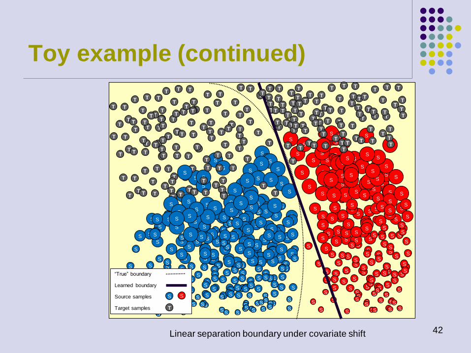
Toy example (continued)

42

S

S

S

S

S

S

S

S

S

S

S

S

S

S

S

S

S

S

S

S

S

S

S

S

S

S

S

S

S

S

S

S

S

S

S

S

S

S

S

S

S

S

S

S

S

S

S

S

S

S

S

S

S

S

S

S

S

S

S

S

S

S

S

S

S

S

S

S

S

S

S

S

S

S

S

S

S

S

S

S

S

S

S

S

S

S

S

S

S

S

S

S

S S

S

S

S

S S S

S

S

S

S

S

S

S

S

S

S

S

S

S

S S

S

S

S

S

S

S

S

S

S

S

S

S

S

S

S

S

S S

S

S

S

S

S

S

S

S

S

S

S

S

S S

S

S

S

S

S

S

S

S

S

S

S

S

S

S

S

S

S

S

S

S

S

S

S

S

S

S

S

S

S

S

S

S

S

S

S

S

S S

S

S

S

S

S

S

S

S

S

S

S

S

S

S

S

S

S

S

S

S

S

S

S

S

S S

S

S

S

S

S

S

S

S

S

S

S

S

S

S

S

S

S

S

S

S

S

S

S

S

S

S

S

S

S

S

S

S

S

S

S

S

S

S

S

S

S

S

S

S

S

S

S

S

S

S

S

S

S

S

S

S

S

S

S

S

S

S

S

S

S

S

S

S

S

S

S

S S

S

S

S

S

S

S

S

S

S

S

S

S

S

S

S

S

S

S

S

S

S S

S

S

S

S

S

S

S

S

S

S

S

S

S

S

S

S

S

S

S

S

S

S

S

S

S

S

S

S

S

S

S

S

S

S

S

S

S

S

S

S

S

S S

S

S

S

S

S S

S S

S

S

S

S

S

S

S

S

S

S

S

S

S

S

S

S

S

S

S

S

S

S

S

S

S

S

S

S

S

S

S

S

S

S

S

S

S

S

S S

S

S

S

S

S

S

S

S

S

S

S

S

S

S

S

S

S

S

S S

S

S

S

S

S

S S

S

S

S

S

S

S

S

S

S S

S

S S

S

S

S

S

S

S S

S

S

S

S

S

S

S

S

S

S

S

S S

S

S

T T

T

T

T T T

T

T

T T

T T T

T

T T

T

T

T

T T

T

T

T

T T

T

T

T T T

T

T

T T T

T

T

T T T

T

T

T

T T

T

T

T T T

T

T

T

T T T

T

T T

T

T

T T T

T

T T T T

T

T

T T

T

T

T T T

T

T T T T

T

T

T T

T

T

T T T

T

T T T T

T

T

T T

T

T

T T T

T

T T T T

T

T

T T

T

T

T

T T

T

T T T T

T

T

T T

T

T

T T T

T

T T T T

T

T

T T

T

T

T T T

T

T T T T

T

T

T T

T

T

T T T

T

T T T T

T

T

S

S

S

S

S

S

S

S S

S

S

S

T

T

T T

T

T T T

T

T T

T

T

T

T

T T

T

T

T

T

T

T T

T

T

T

T

T

T T

T T

T

T

“True” boundary

Learned boundary

S S Source samples

Target samples T

Linear separation boundary under covariate shift

Constraining the model on KS

and CvM values

4. Solution: transfer learning 43

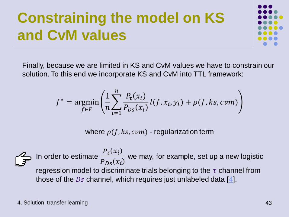
Finally, because we are limited in KS and CvM values we have to constrain our

solution. To this end we incorporate KS and CvM into TTL framework:

𝑓∗ = argmin𝑓∈𝐹

1

𝑛

𝑃𝜏 𝑥𝑖

𝑃𝐷𝑠 𝑥𝑖𝑙(𝑓, 𝑥𝑖 , 𝑦𝑖)

𝑛

𝑖=1

+ 𝜌(𝑓, 𝑘𝑠, 𝑐𝑣𝑚)

where 𝜌(𝑓, 𝑘𝑠, 𝑐𝑣𝑚) - regularization term

In order to estimate 𝑃𝜏 𝑥𝑖

𝑃𝐷𝑠 𝑥𝑖 we may, for example, set up a new logistic

regression model to discriminate trials belonging to the 𝜏 channel from

those of the 𝐷𝑠 channel, which requires just unlabeled data [4].

5. IMPLEMENTATION

44

Implementation

5. Implementation 45

For the competition we have submitted several different models. The transfer

learning model achieved AUC = 0.996802 on Public Leader Board. It was

improved to 0.998150 post competition. Source code can be downloaded from

GitHub page https://github.com/alexander-rakhlin/flavours-of-physics

As we remember, training on 𝐷𝑠 channel was prohibited by the competition

requirements, what dictated us certain amendments to the Transductive

Transfer Learning framework outlined in Section 4.

In this implementation we transfer model from 𝜏 channel to 𝐷𝑠 channel. The

other difference is how domain adaptation is implemented: instead of covariate

shift we do calibration.

Initial training

5. Implementation 46

We implemented two-stage process: 1) Initial training and 2) Adaptation stage.

On the Initial stage the model is trained for maximum performance on labeled

data from 𝜏 channel. This model is based on ensemble of 20 feed forward fully

connected neural nets written in Python with Keras library. Each net comprises

4 fully connected hidden layers F1-F4 with PReLU activations fed to a 2-way

softmax output layer which produces a distribution over the 2 class labels. The

hidden layers contain 75, 50, 30, and 25 neurons respectively. To avoid

overfitting, dropout is used in F1, F2 and F3 layers:

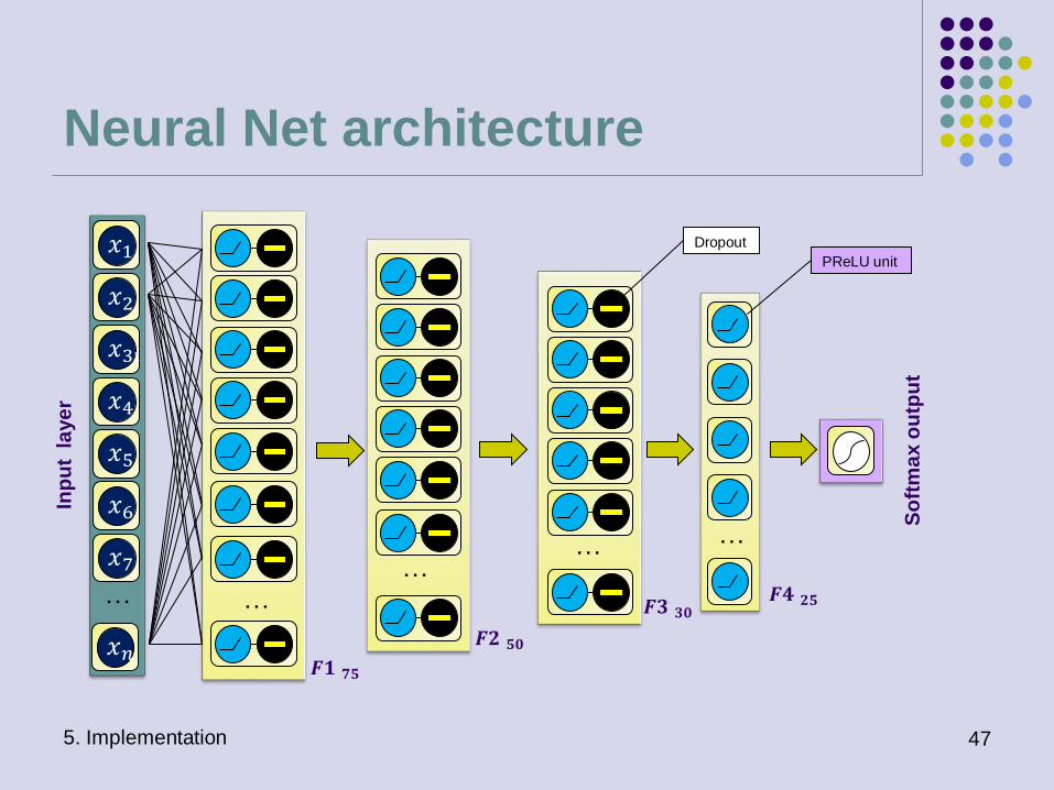
Neural Net architecture

5. Implementation 47

𝑥1

𝑥2

𝑥3𝑖

𝑥4

𝑥5

𝑥6

𝑥7

𝑥𝑛

… …

… … …

So

ftm

ax

ou

tpu

t

Inp

ut

la

ye

r

𝑭𝟏 𝟕𝟓

PReLU unit

Dropout

𝑭𝟐 𝟓𝟎

𝑭𝟑 𝟑𝟎 𝑭𝟒 𝟐𝟓

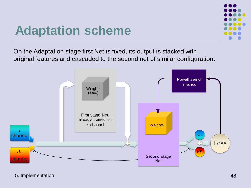
Adaptation scheme

5. Implementation

First stage Net, already trained on

𝜏 channel

Second stage Net

AUC

KS

Loss

Powell search

method

Weights

Weights (fixed)

On the Adaptation stage first Net is fixed, its output is stacked with

original features and cascaded to the second net of similar configuration:

𝜏 channel

𝐷𝑠

channel

48

Training the 2-nd Net

5. Implementation 49

𝐷𝑠 channel was labeled for other purpose than training, and training on 𝐷𝑠

was prohibited. But calculation of KS and CvM values - allowed. The other

metric to satisfy is AUC on 𝜏 channel. All 3 metrics are global and do not

suit for stochastic gradient descent (SGD). Therefore we train this second

Net in a special way (see code):

1. We set initial weights of the second Net to reproduce output of the first

Net. This is accomplished after 1-3 epochs of SGD with cross entropy

loss on 𝜏 samples.

2. Then adaptation of weights is done with help of Powell’s search method in minimize() function from scipy.optimize library. On this step

the Net is fed with 𝜏 and 𝐷𝑠 samples and optimized directly for AUC, KS

and CvM metrics.

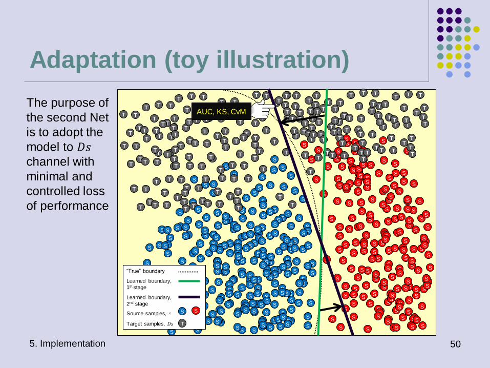
Adaptation (toy illustration)

50

The purpose of

the second Net

is to adopt the

model to 𝐷𝑠

channel with

minimal and

controlled loss

of performance

5. Implementation

S

S

S

S

S

S

S

S

S

S

S

S

S

S

S

S

S

S

S

S

S

S

S

S

S

S

S

S

S

S

S

S

S

S

S

S

S

S

S

S

S

S

S

S

S

S

S

S

S

S

S

S

S

S

S

S

S

S

S

S

S

S

S

S

S

S

S

S

S

S

S

S

S

S

S

S

S

S

S

S

S

S

S

S

S

S

S

S

S

S

S

S

S

S

S

S

S

S S S

S

S

S

S

S

S

S

S

S

S

S

S

S

S

S

S

S

S

S

S

S

S

S

S

S

S

S

S

S

S

S

S S

S

S

S

S

S

S

S

S

S

S

S

S

S

S

S

S

S

S

S

S

S

S

S

S

S

S

S

S

S

S

S

S

S

S

S

S

S

S

S

S

S

S

S

S

S

S

S

S

S

S

S

S

S

S

S

S

S

S

S

S

S

S

S

S

S

S

S

S

S

S

S

S

S

S

S

S

S

S

S

S

S

S

S

S

S

S

S

S

S

S

S

S

S

S

S

S

S

S

S

S

S

S

S

S

S

S

S

S

S

S

S

S

S

S

S

S

S

S

S

S

S

S

S

S

S

S

S

S

S

S

S

S

S

S

S

S

S

S

S

S

S

S

S

S

S

S

S

S

S

S S

S

S

S

S

S

S

S

S

S

S

S

S

S

S

S

S

S

S

S

S

S

S

S

S

S

S

S

S

S

S

S

S

S

S

S

S

S

S

S

S

S

S

S

S

S

S

S

S

S

S

S

S

S

S

S

S

S

S

S

S

S

S

S

S S

S

S

S

S

S S

S

S

S

S

S

S

S

S

S

S

S

S

S

S

S

S

S

S

S

S

S

S

S

S

S

S

S

S

S

S

S

S

S

S

S

S

S

S

S

S

S S

S

S

S

S

S

S

S

S

S

S

S

S

S

S

S

S

S

S

S

S

S

S

S

S

S

S S

S

S

S

S

S

S

S

S

S S

S

S S

S

S

S

S

S

S S

S

S

S

S

S

S

S

S

S

S

S

S S

S

S

T T

T

T

T T T

T

T

T T

T T T

T

T T

T

T

T

T T

T

T

T

T T

T

T

T T T

T

T

T T T

T

T

T T T

T

T

T

T T

T

T

T T T

T

T

T

T T T

T

T T

T

T

T T T

T

T T T T

T

T

T T

T

T

T T T

T

T T T T

T

T

T T

T

T

T T T

T

T T T T

T

T

T T

T

T

T T T

T

T T T T

T

T

T T

T

T

T

T T

T

T T T T

T

T

T T

T

T

T T T

T

T T T T

T

T

T T

T

T

T T T

T

T T T T

T

T

T T

T

T

T T T

T

T T T T

T

T

S

S

S

S

S

S

S

S S

S

S

S

T

T

T T

T

T T T

T

T T

T

T

T

T

T T

T

T

T

T

T

T T

T

T

T

T

T

T T

T T

T

T

“True” boundary

Learned boundary,

1st stage

S S Source samples,

Target samples, 𝐷𝑠 T

Learned boundary,

2nd stage

AUC, KS, CvM

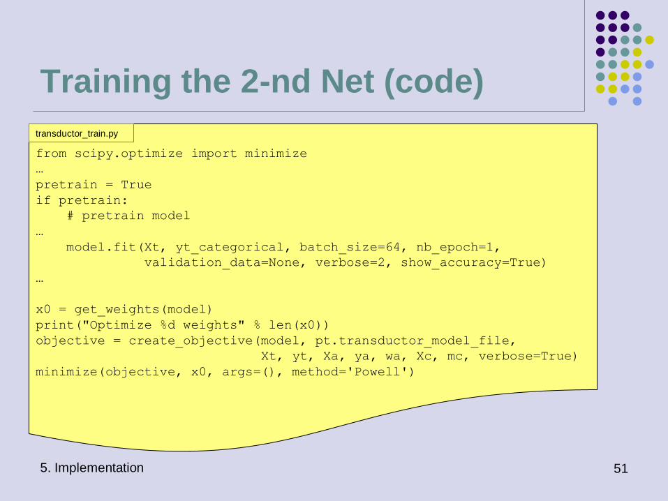
Training the 2-nd Net (code)

5. Implementation 51

from scipy.optimize import minimize

…

pretrain = True

if pretrain:

# pretrain model

…

model.fit(Xt, yt_categorical, batch_size=64, nb_epoch=1,

validation_data=None, verbose=2, show_accuracy=True)

…

x0 = get_weights(model)

print("Optimize %d weights" % len(x0))

objective = create_objective(model, pt.transductor_model_file,

Xt, yt, Xa, ya, wa, Xc, mc, verbose=True)

minimize(objective, x0, args=(), method='Powell')

transductor_train.py

Loss function

5. Implementation 52

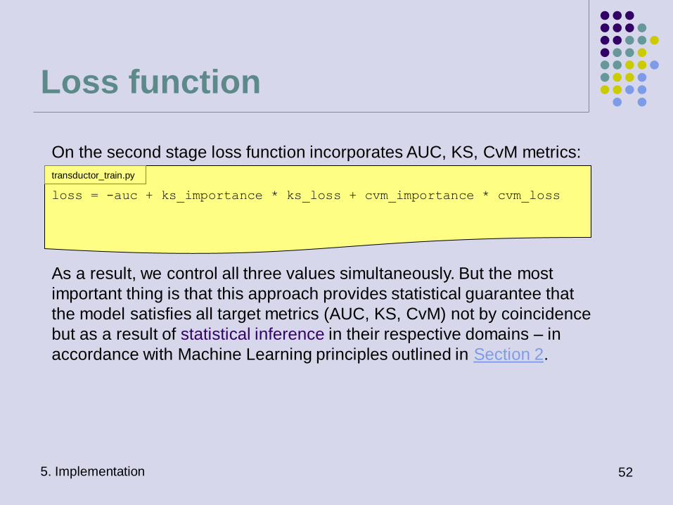
On the second stage loss function incorporates AUC, KS, CvM metrics:

As a result, we control all three values simultaneously. But the most

important thing is that this approach provides statistical guarantee that

the model satisfies all target metrics (AUC, KS, CvM) not by coincidence

but as a result of statistical inference in their respective domains – in

accordance with Machine Learning principles outlined in Section 2.

loss = -auc + ks_importance * ks_loss + cvm_importance * cvm_loss

transductor_train.py

Closing remarks and suggestions

5. Implementation 53

The model appears more complex than it should be! Striving to satisfy some

competition requirements we overdone fairly simple Transfer Learning

Framework. We encourage the Organizers to lift “no training on control

channel” requirement and try to create a model the other way round: on 𝐷𝑠

channel and transfer it to 𝜏 channel…. If this has physical meaning, of course

In general, we suggest to consider transfer learning as a method for

modeling rare events based on models built in domains with more known

and well-observed behavior.

Some other ML approaches to consider for rare events detection [11]:

• One-class classification (a.k.a. outlier detection, anomaly detection,

novelty detection)

• PU learning

References

[1] Blake T., Bettler M.-O., Chrzaszcz M., Dettori F., Ustyuzhanin A., Likhomanenko T., “Flavours of Physics: the

machine learning challenge for the search of 𝜏-→𝜇-𝜇-𝜇+ decays at LHCb” link

Machine Learning:

[2] Y. S. Abu-Mostafa, H.-T. Lin, M. Magdon-Ismail, “Learning From Data”. AMLBook (March 27, 2012), ISBN-10:

1600490069

[3] Andrew Ng, “Part VI Learning Theory”. Stanford University CS229 Lecture notes link

Transfer learning:

[4] Olivetti, E., Kia, S.M., Avesani, P.: “Meg decoding across subjects.” In: Pattern Recognition in Neuroimaging, 2014

International Workshop on (2014) link

[5] S. J. Pan and Q. Yang, “A Survey on Transfer Learning,” Knowledge and Data Engineering, IEEE Transactions on,

vol. 22, no. 10, pp. 1345–1359, Oct. 2010.

[6] B. Zadrozny, “Learning and Evaluating Classifiers under Sample Selection Bias” In Proceedings of the Twenty-first

International Conference on Machine Learning, ser. ICML ’04. New York, NY, USA: ACM, 2004, pp. 114+.

[7] Jiang J., “A Literature Survey on Domain Adaptation of Statistical Classifiers” link

[8] Adel T., Wong A., “A Probabilistic Covariate Shift Assumption for Domain Adaptation”. In Proceedings of the

Twenty-Ninth AAAI Conference on Artificial Intelligence link

References 54

References (continued)

Kolmogorov-Smirnov test:

[9] Wikipedia, “Kolmogorov–Smirnov test” link

[10] Andrew P. Bradley, “ROC Curve Equivalence using the Kolmogorov-Smirnov Test”. The University of Queensland,

School of Information Technology and Electrical Engineering, St Lucia, QLD 4072, Australia link

Other methods:

[11] Wikipedia, “One-class classification” link

References 55

Acknowledgements

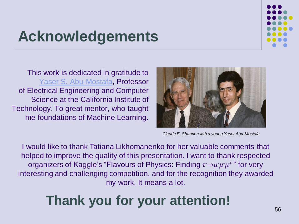
This work is dedicated in gratitude to

Yaser S. Abu-Mostafa, Professor

of Electrical Engineering and Computer

Science at the California Institute of

Technology. To great mentor, who taught

me foundations of Machine Learning.

56

Claude E. Shannon with a young Yaser Abu-Mostafa

Thank you for your attention!

I would like to thank Tatiana Likhomanenko for her valuable comments that

helped to improve the quality of this presentation. I want to thank respected

organizers of Kaggle’s “Flavours of Physics: Finding 𝜏-→𝜇-𝜇-𝜇+ ” for very

interesting and challenging competition, and for the recognition they awarded

my work. It means a lot.