flight validation of metrics driven l1 adaptive control

Flight Validation

of a Metrics Driven L1 Adaptive Control

Vladimir Dobrokhodov∗, Ioannis Kitsios†, Isaac Kaminer‡, Kevin D. Jones§

Naval Postgraduate School, Monterey, CA 93943

Enric Xargay¶, Naira Hovakimyan‖

University of Illinois at Urbana-Champaign, Urbana, IL 61801

Chengyu Cao ∗∗

University of Connecticut, Stoors, CT 06269

Mariano I. Lizarraga ††

UC Santa Cruz, Santa Cruz, CA 95064

Irene M. Gregory ‡‡

NASA Langley Research Center, Hampton, VA 23681

The paper addresses initial steps involved in the development and flight implementationof new metrics driven L1 adaptive flight control system. The work concentrates on (i)definition of appropriate control driven metrics that account for the control surface failures;(ii) tailoring recently developed L1 adaptive controller to the design of adaptive flightcontrol systems that explicitly address these metrics in the presence of control surfacefailures and dynamic changes under adverse flight conditions; (iii) development of a flightcontrol system for implementation of the resulting algorithms onboard of small UAV; and(iv) conducting a comprehensive flight test program that demonstrates performance of thedeveloped adaptive control algorithms in the presence of failures. As the initial milestonethe paper concentrates on the adaptive flight system setup and initial efforts addressingthe ability of a commercial off-the-shelf autopilot with and without adaptive augmentationto recover from control surface failures.

I. Introduction

Aircraft loss-of-control (LOC) accidents1,2 comprise a significant aircraft accident category across allcivil transport classes, and can result from a large array of causal and contributing factors occurring eitherindividually or, most likely, in combination. According to the National Transportation Safety Board’saccident database3–6 , 40% of all the commercial aviation fatalities from 1990 – 1996 were due to a LOC7 .Causes for LOC can come from multiple sources, such as:

• Inadequate input from the pilot: In Comair’s air taxi and commuter airplane EMB-120T accidentthe flightcrew’s decision to operate in icing conditions near the lower margin of the operating airspeedenvelope caused wing’s icing and the subsequent LOC which resulted in 29 fatalities.

∗Research Assistant Professor, Dept. of Mech. & Astronautical Eng., AIAA Member; [email protected].†Postdoctoral Research Fellow, Dept. of Mech. & Astronautical Eng. , Cpt (HAF); [email protected].‡Professor, Dept. of Mech. & Astronautical Eng., member AIAA; [email protected].§Research Associate Professor, Dept. of Mech. & Astronautical Eng., AIAAAssociate Fellow; [email protected].¶Graduate Student, Dept. of Mechanical Science and Engineering, AIAA Student Member; [email protected].‖Professor, Dept. of Mechanical Science and Engineering, Associate Fellow AIAA; [email protected].∗∗Assistant Professor, Dept. of Mechanical Engineering, AIAA Member; [email protected].††Graduate student, Baskin School of Engineering, AIAA Student Member; [email protected].‡‡Senior Aerospace Research Engineer, Dynamic Systems and Controls Branch, MS 308, AIAA Senior Member;

[email protected].

1 of 22

American Institute of Aeronautics and Astronautics

AIAA Guidance, Navigation and Control Conference and Exhibit18 - 21 August 2008, Honolulu, Hawaii

AIAA 2008-6987

This material is declared a work of the U.S. Government and is not subject to copyright protection in the United States.

• Control surface failure: In US Air’s Boeing-737 the LOC resulting from the movement of the ruddersurface to its blowdown limit as a result of a jam of the main rudder power control unit servo resultedin 132 fatalities.

• Equipment damage: In Alaska Airlines MD-83 the LOC resulting from the in-flight failure of thehorizontal stabilizer trim system jackscrew assembly’s acme nut threads resulted in 88 fatalities.

• Change in flight characteristics of the aircraft: In American Eagle Airlines ATR-72-212 wherea LOC attributed to a sudden and unexpected aileron hinge moment reversal that occurred after aridge of ice accreted beyond the deice boots while the airplane was in a holding pattern resulted in 68fatalities.

Further study of these and many more LOC accidents performed by NASA-Langley and other researchcenters determined that often pilots trying to recover from a LOC typically found themselves trying to flythe airplanes out of the normal operational flight envelope and in attitudes where they typically were nottrained to fly8 . Figure 1 shows how a LOC accident puts the aircraft in the attitude well beyond the windtunnel data envelope of what is considered a “normal” flight condition.

Figure 1: Loss of control accident data relative to angle of attack and angle of sideslip7

When a failure occurs, the following critical questions must be addressed: is the failure severe enoughthat only stability can be maintained to land the aircraft anywhere possible (loss of vertical tail in DC-10in Sioux City Iowa) or is there sufficient control authority left to provide a measure of performance (engineout with sufficient rudder authority)? In the case of a severe failure, when only stability can be maintained,the control metrics that must be assessed include controllability and stability margins. Due to significantdegradation of the flight envelope controllability bounds may no longer be symmetric, for example, left andright bank angles may be different. Clearly, the adaptive control system employed must guarantee thatthe new limits on dynamic maneuverability and limits on the remaining control surfaces and throttles arenot violated for the remainder of the flight for the known initial conditions and in the presence of boundeddisturbances. This clearly motivates the use of recently developed L1 adaptive control theory9,10 as a naturalmetric for the analysis of the adaptive control system. Furthermore, due to the presence of adaptive controlthe resulting feedback system is necessarily nonlinear, which requires the use of time-delay margin as ameasure of robustness instead of the standard phase margin, typical of linear systems.

On the other hand, if the failure is less severe and a certain level for performance can be maintained,new metrics (in addition to the ones discussed above) can be used to assess performance of the adaptivecontrol system. Clearly, the most important one would be landing the aircraft on a given runway. Thus

2 of 22


the adaptive control system must follow a predefined feasible path and must guarantee that the predictedlateral miss distance does not exceed the width of the runway. Therefore, the lateral miss distance at thetouch down is a critical metric that must be used to evaluate performance of the adaptive control system.In addition, a certain modicum of passenger comfort such as lateral and normal g loads should not exceedsome predefined bounds (depending on the nature of the failure) throughout the remainder of the flight inthe presence of bounded disturbances and for given initial conditions. Again this motivates the use of therecently developed L1 adaptive control theory as a metric par excellence to evaluate the maximum g-loadingproduced by the actions of the adaptive control system.

In general, an actual LOC accident takes the airplane beyond the normal flight envelope into regions forwhich aerodynamic data are not available from conventional sources (see Fig. 1). There is still limitation ofmodeling aerodynamic force and moments at high angles of attack due to time-dependent effects, unsteadyaero-effects, and the Reynolds number effects on wind tunnel test data. Figure 1 shows that the flighttest data are not matched with the wind tunnel data at conventional stall angle of attack. There is alsolimitation on modeling the effects of the loss of control effectiveness on aircraft dynamics. Furthermore, theaerodynamic changes due to either individual actuator failure or combination of several actuators may notbe adequately modeled a priori. Thus, lack of adequacy in modeling requires an application of new adaptivecontrol algorithm and also stresses the importance of system identification methods, particular for the caseof multidimensional systems.

The theory and practice of aircraft system identification has a long history and is very well estab-lished11–13 . Modern computational methods, wind-tunnel and flight testing can provide comprehensive dataabout the aerodynamic characteristics of an aircraft. Variety of existing numerical and experimental methodsand techniques is classified so that a researcher has a well-defined roadmap to be used in choosing the rightmethod and its application. Yet, many authors concur (see subject area review in Ref.11) that althoughmethods exist there is still room for new identification techniques and there exist many regimes and charac-teristics yet to be identified. New aerodynamic configurations, engines and flight control modes, without evenaccounting for LOC due to control surfaces failures (CSF), make system identification area active as neverbefore. In particular for the problem at hand, system identification contributes to the design of adaptivestability augmentation system through (i) obtaining more accurate and comprehensive mathematical modelof aircraft dynamics used at the design and simulation stages, and (ii) providing verifiable estimates of theremaining control authority when any adverse conditions occur.

Near optimal trajectory generation is another task to be solved online. Many advances have been madein recent years in this area; a comprehensive overview can be found in Refs.14,15 . In the event of LOC,optimizing feasible path is of paramount importance. It should not only account for remaining controlauthority but must allow for near real time reconfiguration of the projected path. Furthermore, safetyof the computational system is another important issue that must be addressed; in the presence of finitecomputation time, by analyzing the behavior of the implemented algorithms, the CPU time planning mustbe also performed in real time to guarantee safety of computation16 . In application to the problem at handthe most computationally inexpensive modification17 of the direct method of calculus of variations is used.The method allows for real-time computation of feasible trajectories and delivers near real-time suboptimalsolutions subject to a multidimensional constraints on control functions, initial and final conditions. Onboardimplementation of this method is numerically inexpensive and has been proven robust in various applicationsand flight experiments17–19 .

Furthermore, over the years, unmanned aerial vehicles (UAVs) have played increasingly important roles inthe development of novel aircraft technologies. These vehicles are typically viewed as tools which provide low-risk and low-cost means for testing new advanced concepts. Over the span of last 20 years, as computationalpower has grown by leaps and bounds and the packaging of onboard electronics has been significantlyminiaturized, UAVs are being viewed with increased interest to perform a variety of new research missions.

The framework proposed for current development borrows from multiple disciplines and integrates of-fline algorithms for system identification, and online algorithms for path generation, path following, andL1 adaptive control theory for fast and robust adaptation. Together, these techniques yield control laws thatmeet strict performance requirements in the presence of CSF, modeling uncertainties and environmentaldisturbances. The methodology proposed for this work unfolds in three basic steps. First, given a nominalUAV (no CSF implemented) in wings level flight, a feasible trajectory is generated onboard for a given setof initial (grabbed in flight) and final boundary conditions (assigned a priori according to the scenario), ageneral performance criterion to be optimized, and the simplified UAV dynamics.

3 of 22


Next, as soon as a near optimal trajectory for nominal aircraft is generated in real time, the UAV isautomatically transitioned to the path following mode with zero initial tracking errors. The path followingcontrol algorithm proposed builds on a nonlinear control strategy, which is first derived at a kinematiclevel, and leads to an outer-loop controller that generates pitch and yaw rate commands to an inner-loopcontroller. At a second level, the dynamics of the closed-loop UAV with autopilot (AP) are dealt with byintroducing an inner-loop control law via the L1 adaptive output feedback controller wrapped around theautopilot. This L1 adaptive augmentation is what allows us to account for the UAV dynamics, guaranteeingstability and performance of the complete system in the presence of modeling uncertainties and environmentaldisturbances. The main benefit of the L1 adaptive controller is its ability of fast and robust adaptation, asproven in Refs.9,10,20–23 , which leads to desired transient and steady-state performance for system’s bothinput and output signals simultaneously, in addition to guaranteed gain and time-delay margins9,10 . Thethird step consists of introducing CSF while in path following mode and verying the performance metricsof L1 adaptive controller in real flight. It is done without acknowledging the nominal AP about the failureand therefore without reconfiguring the nominal inner-loop controller; AP continues to send commands tothe control surface that is fixed at the specified position. The ultimate objective is therefore to estimate theboundary of the achievable tracking performance with the most severe CSF deflection.

Thus, L1 adaptive control theory will be considered as the framework for the development and validationof the metric driven adaptive control paradigm. Previous work and theoretical details of L1-adaptive controltheory, known as The Theory of Fast and Robust Adaptation, are presented next in Section II. Motivation anddevelopment of a new hardware in the loop flight simulator providing advanced flight modeling capabilitiesfollows next in Section III. Section IV concentrates on the preliminary development of flight test failurematrix including single and multiple CSF, and presents corresponding HIL simulation results. Finally,Section V describes the results of the flight test experimentation program implementing CSFs and theadaptive control algorithm onboard of the SUAV. The paper ends with the concluding remarks in Section VI.

II. Path Following and L1 Adaptive Control

A. Path Following Problem Formulation

This section briefly formulates the problem of path following control for a (single) UAV in 3D space. Werecall that path following refers to the problem of making a vehicle converge to and follow a desired feasiblepath described by some convenient time-independent parameter (e.g., path length).

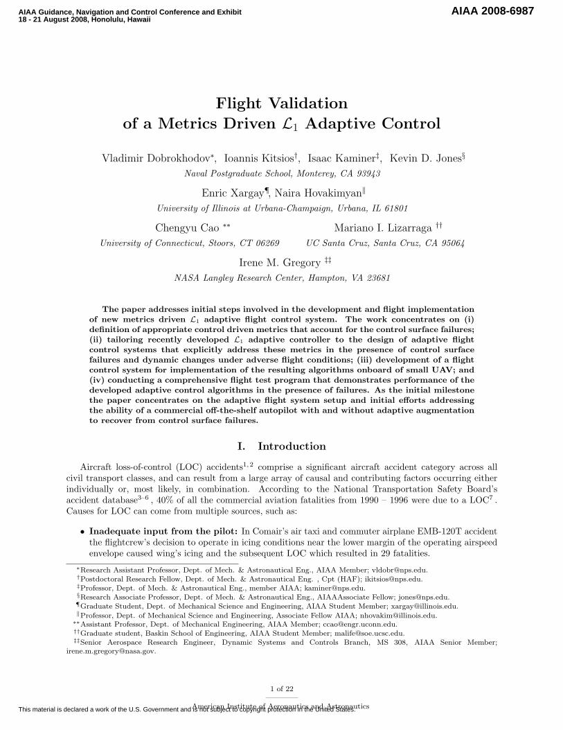
In previous work by the authors (Refs.24,25) a general framework for this problem is proposed. In theset-up adopted, the kinematic model of the vehicle is derived with respect to a Serret-Frenet frame movingalong the path, playing the role of a virtual target vehicle to be tracked by the real vehicle. The key ideainvolved in the approach is to consider the rate of progression of the virtual target as a degree of freedom,which in turn allows to decouple spatial and temporal assignments during the path generation and pathfollowing phases. The geometry of the problem at hand is shown in Figure 2. Given a path pc(l) to befollowed, parameterized by a path length l, we define Q to be the UAV center of mass and P to be anarbitrary point on the path that plays the role of the center of mass of a virtual UAV to be followed. Wealso define the path following kinematic position-error vector qF (t) as the difference between the position ofthe UAV center of mass Q and the position of the virtual UAV P (resolved in F), which is represented as

qF (t) = [ xF (t) yF (t) zF (t) ]> ,

and the path following kinematic attitude-error vector Φe(t) as the vector of Euler angles that locally pa-rameterize the rotation matrix from F to a coordinate systemW ′ defined by projecting the wind frame ontoa local level plane

Φe(t) = [ φe(t) θe(t) ψe(t) ]> .

Then, as shown in Ref.25 , the overall open-loop path following system including the autopilot and theaircraft dynamics can be described by a cascaded structure of the form

Ge : x(t) = f(x(t)) + g(x(t))y(t) (1)Gp : y(s) = Gp(s)(u(s) + z(s)) , (2)

4 of 22


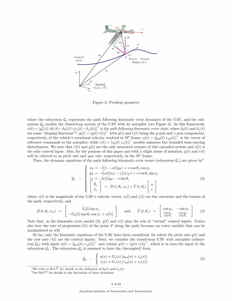
Figure 2: Problem geometry

where the subsystem Ge represents the path following kinematic error dynamics of the UAV, and the sub-system Gp models the closed-loop system of the UAV with its autopilot (see Figure 3). In this framework,x(t) = [q>F (t) (θe(t)−δθ(t)) (ψe(t)−δψ(t))]> is the path following kinematic error state, where δθ(t) and δψ(t)are some “shaping functions”a; y(t) = [q(t) r(t)]> with q(t) and r(t) being the y-axis and z-axis components,respectively, of the vehicle’s rotational velocity resolved in W ′ frame; u(t) = [qad(t) rad(t)]> is the vector ofreference commands to the autopilot; while z(t) = [zq(t) zr(t)]> models unknown but bounded time-varyingdisturbances. We note that x(t) and y(t) are the only measured outputs of this cascaded system and u(t) isthe only control input. Also, for the purpose of this paper and with a slight abuse of notation, q(t) and r(t)will be referred to as pitch rate and yaw rate, respectively, in the W ′ frame.

Then, the dynamic equations of the path following kinematic error states (subsystem Ge) are given byb

Ge :

xF = −l(1− κ(l)yF ) + v cos θe cosψeyF = −l(κ(l)xF − ζ(l)zF ) + v cos θe sinψezF = −lζ(l)yF − v sin θe[θe

ψe

]= D (t, θe, ψe) + T (t, θe)

[q

r

] (3)

where v(t) is the magnitude of the UAV’s velocity vector, κ(l) and ζ(l) are the curvature and the torsion ofthe path, respectively, and

D (t, θe, ψe) =

[lζ(l) sinψe

−l(ζ(l) tan θe cosψe + κ(l))

]and T (t, θe) =

[cosφe − sinφesinφe

cos θe

cosφe

cos θe

]. (4)

Note that, in the kinematic error model (3), q(t) and r(t) play the role of “virtual” control inputs. Noticealso how the rate of progression l(t) of the point P along the path becomes an extra variable that can bemanipulated at will.

So far, only the kinematic equations of the UAV have been considered, for which the pitch rate q(t) andthe yaw rate r(t) are the control inputs. Next, we consider the closed-loop UAV with autopilot (subsys-tem Gp) with input u(t) = [qad(t) rad(t)]> and output y(t) = [q(t) r(t)]>, which is in turn the input to thesubsystem Ge. The subsystem Gp is assumed to have the (decoupled) form

Gp :

q(s) = Gq(s) (qad(s) + zq(s))r(s) = Gr(s) (rad(s) + zr(s))

(5)

aWe refer to Ref.25 for details in the definition of δθ(t) and δψ(t).bSee Ref.24 for details in the derivation of these dynamics.

5 of 22


UAV with Autopilot

Path FollowingKinematics

A/P UAV

Figure 3: Cascaded path following error dynamics with UAV dynamics

where Gq(s), Gr(s) are unknown strictly proper and stable transfer functions and zq(s), zr(s) represent theLaplace transforms of zq(t) and zr(t), respectively. In Ref.25, we justify the adoption of a linear time-invariantmodel for the UAV together with its autopilot.

Then, given a desired path to be followed, the control objective is to stabilize x(t) by proper design ofu(t) without any modifications to the autopilot.

B. Stabilizing Function for the Path Following Kinematics (outer-loop)

As shown in Ref.25, in the ideal case where Gp is the identity operator, if the rate of progression of thepoint P along the path is appropriately chosen, then there exist stabilizing functions qc(t) and rc(t) for q(t)and r(t), respectively, leading to local exponential stability of the origin of Ge with a prescribed domain ofattraction. A formal statement of this semi-global result is given in the lemma below.

Lemma 1 Let the progression of the point P along the path be governed by

l = K1xF + v cos θe cosψe , (6)

where K1 > 0, and define the input vector yc(t) as

yc =

[qc

rc

]= T−1 (t, θe)

([uθc

uψc

]−D (t, θe, ψe)

), (7)

where uθc(t) and uψc

(t) are given by

uθc = −K2(θe − δθ) +c2c1zF v

sin θe − sin δθθe − δθ

+ δθ

uψc= −K3(ψe − δψ)− c2

c1yF v cos θe

sinψe − sin δψψe − δψ

+ δψ (8)

with some K2, K3, c1, c2 > 0c. Then, there exist a domain of attraction Ω such that the kinematic errorequations in (3) with the controllers q(t) ≡ qc(t), r(t) ≡ rc(t) defined in (7)-(8) are exponentially stable.

Proof. The proof of this Lemma can be found in Ref.25 .

C. L1 Adaptive Output-Feedback Augmentation (inner-loop)

The variables qc(t) and rc(t) generated by the (outer-loop) path following algorithm must be viewed ascommands to be tracked by appropriately designed inner-loop control systems. Since commercial autopilotsare normally designed to track simple way-point commands, the pitch and yaw rate commands computed

cWe refer to Ref.25 for details in the choice of the parameters K1, K2, K3, c1, and c2.

6 of 22


ControlLaw

StatePredictor

AdaptiveLaw

System

Augmentation

Figure 4: L1 adaptive augmentation loop for pitch rate control

before are modified by including an L1-adaptive loop to ensure that the closed-loop UAV with the autopilottracks the commands qc(t) and rc(t) following desired reference models Mq(s), and Mr(s) i.e.

q(s) ≈ Mq(s)qc(s) and r(s) ≈ Mr(s)rc(s) ,

where Mq(s) and Mr(s) are designed to meet the desired specifications. In this paper, for simplicity, weconsider a first order system, by setting

M•(s) =m•

s+m•, m• > 0 .

The philosophy of the L1 adaptive output feedback controller is to obtain an estimate of the uncertaintiesof the plant, and define a control signal which compensates for these uncertainties within the bandwidth of alow-pass filter C(s) introduced in the feedback loop. This filter represents the key difference of L1 adaptivecontrol from conventional MRAC, and guarantees that the L1 adaptive controller stays in the low-frequencyrange even in the presence of high adaptive gains and large reference inputs. The choice of C(s) defines thetrade-off between performance and robustness10 . Adaptation is based on the projection operator, ensuringboundedness of the adaptive parameters by definition, and uses the output of a state predictor to update theestimate of the uncertainties. The L1 adaptive control architecture for the pitch-rate channel is representedin Figure 4 and its elements are introduced below.

State Predictor: We consider the state predictor

˙q(t) = −mq q(t) +mq (qad(t) + σq(t)) , q(0) = q(0) , (9)

where the adaptive estimate σq(t) is governed by the following adaptation law.Adaptive Law: The adaptation of σq(t) is defined as

˙σq(t) = ΓcProj(σq(t),−q(t)), σq(0) = 0, (10)

where q(t) = q(t)−q(t) is the error between the state predictor and the output of the actual system, Γc ∈ R+

is the adaptation rate subject to a computable lower bound, and Proj denotes the projection operator26 .Control Law: The control signal is generated by

qad(s) = Cq(s) (rq(s)− σq(s)) , (11)

where rq(t) is a bounded reference input signal with bounded derivative, and Cq(s) is a strictly properlow-pass filer with Cq(0) = 1. In this paper, we consider the simplest choice of a first order filter

Cq(s) =ωq

s+ ωq, ωq > 0 .

7 of 22


The complete L1 adaptive output feedback controller consists of (9), (10) and (11), with Mq(s) and Cq(s)ensuring stability ofd

H(s) =Gq(s)Mq(s)

Cq(s)Gq(s) + (1− Cq(s))Mq(s). (12)

Then, given the L1 adaptive augmentation above, it is possible to derive a performance bound forsystem’s output q(t) with respect to the reference command qc(t). Next lemma states this key result. Weavail ourselves of previous work on L1 augmentation and its application to path following23,25 .

Lemma 2 Let rq(t) be a bounded reference command with bounded derivative. Given the L1 adaptive con-troller defined via (9), (10) and (11) subject to (12), if the adaptation gain Γc and the projection bounds areappropriately chosene, then we have

‖q − rq‖L∞ ≤ γθ with limΓc→∞ωq→∞mq→∞

γθ = 0 .

Proof. The proof of this Lemma can be found in Ref.25 .

Similarly, if we implement the L1 adaptive controller for the yaw-rate channel, with a similar bound forthe initial condition on the yaw-rate, we can derive

‖r − rc‖L∞ ≤ γψ (13)

with γψ > 0 being a constant similar to γθ.

D. Path Following with L1 Adaptive Augmentation

As proven in Ref.,25 the path following closed-loop system with the L1 augmentation (see Figure 5) is stable.In particular, the L1 adaptive augmentation ensures that the outer-loop path following commands qc(t) andrc(t) and their derivatives qc(t) and rc(t) are bounded, which in turn allows to prove that the original domainof attraction for the kinematic error equations Ω can be retained. This key result is stated next.

Theorem 1 Let the progression of the point P along the path be governed (6). For a sufficiently highadaptation gain Γc, there exist control parameters ω, and m such that the (nonlinear) control laws qc(t) andrc(t) in Lemma 1 are bounded with bounded derivatives, and moreover they ensure that, if x(0) ∈ Ω, thenx(t) ∈ Ω for all t ≥ 0, and thus the path following closed-loop cascaded system is ultimately bounded.

Proof. The proof of this Theorem can be found in Ref.25 .

Remark 1 We notice that the approach proposed is different from common backstepping-type analysis forcascaded systems. The advantage of the above structure for the feedback design is that it retains the propertiesof the autopilot, which is designed to stabilize the inner-loop. As a result, it leads to ultimate boundednessinstead of asymptotic stability. From a practical point of view, the procedure adopted for inner/outer loopcontrol system design is quite versatile in that it adapts itself to the particular autopilot installed on-boardthe UAV.

III. Hardware in the Loop and Flight Test Setup

A. Motivation and Development of New HIL Simulator: Architecture Description and Ca-pabilities

Many of the current Commercial Off-The-Shelf (COTS) autopilots offer software simulators to performHIL development, testing and training. Although these simulators work well in general, they are quite

dThis stability condition is a simplified version of the original condition derived in Ref.23 , where the problem formulationincludes output dependent disturbance signals z(t) = f(t, y(t)).

eSee Ref.25 for a detailed discussion and derivation of the design constraints on the adaptation gain Γc, the bandwidth ofthe low-pass filter ωq , and the bandwidth of the state-predictor mq .

8 of 22


Path FollowingKinematicsA/P UAV

Path Following Control

Algorithm

AdaptiveControl

Figure 5: Closed-loop cascaded system with L1 adaptive augmentation

limited when one tries to simulate complicated phenomena or use non-standard aerodynamics. For instance,simulating CSF, a combination of failures or employing a different plant model from the one pre-programmedis simply not possible using these products.

Due to these limitations, the task of developing a new, more versatile HIL simulator, was recentlyaccomplished. The newly developed HIL simulator has the ability to simulate any dynamic model usingSimulink.27 In general, this model is used to generate synthetic sensor data for the autopilot and has thepossibility to receive back control commands directly from the AP. This set up offers flexibility not previouslyavailable in standard Piccolo28 setup and, provided that a plant model obtained by system identification(see Section B) is accurate, reduces the amount of parameter tuning when transitioning from HIL to realflight implementation.

The Piccolo Plus AP28 is the core element of the current Rapid Flight Test Prototyping System (RFTPS)29,30

developed at the NPS. This AP interacts with its own HIL simulator via a Controller Area Network (CAN)bus. It is able to send control surface commands and receive simulated sensor readings from a PC via aCAN to USB converter cable. In order to replace the standard Piccolo Simulator with a new Simulink-basedone two main components were necessary to build: an interface to the CAN/USB data bus and a 6-DOFdynamic model. The complete HIL architecture is shown next in Fig. 6 and the components of this new HILsimulator are described in more detail in the following subsections.

1. Simulation PC

The simulation PC is responsible for generating coherent sensor data for the AP and responding to the APcommands in real time. It consists of two main components: a USB-UDP converter and the 6-DOF Simulinkmodel.

The USB-UDP converter is an application developed in C++. It reads the incoming control surfacecommands from the AP (via USB) and writes them to a UDP port for Simulink model. It also listens to aUDP port where it receives sensor readings data from Simulink model in a predefined format, parses thesereadings and sends them back to the AP via USB.

Simulink is “an environment for multidomain simulation and Model-Based Design for dynamic systems”27

and therefore is a natural choice for a simulation engine. To this end, a Simulink blockset was developedconsisting of two components: (i) a source which listens on a predefined UDP port and parses messages inorder to translate them into the control surface commands (up to 10 different control surfaces); and (ii) asink, with inputs for the traditional sensors (accelerometers, gyros, magnetometers, GPS, dynamic and staticpressure, temperature, engine RPM). This sink parses the data and writes it back to a predefined UDP portin the correct format.31

This setup alone fully replicates the standard capability of the Piccolo HIL Simulator and also extendsit by making use of the flexibility of Simulink as a powerful simulation environment.

9 of 22


Piccolo AP

USB -UDP

Converter

Simulink 6-DOFModelControl Surfaces

Commands

Sensor DataData From/To

Piccolo AP

Simulation PC

PC-104

Aircraft Telemetry

ControlCommands

Operator Interface PC

Logging Data

Control Algorithm Conguration

Simulink Conguration GUI and Data Logging

Piccolo OperatorInterface

PiccoloGroundStation

Wireless Link

Figure 6: HIL setup; new Simulink-based 6DOF model is a centerpiece of the Simulator

2. Operator Interface PC

The Operator Interface (OI)28 is a standard software component of Piccolo-based setup. The OI providesfunctionality to configure the AP gains, set navigation waypoints, monitor the sensor data and display theUAV in a geo-referenced map. It is connected to the Piccolo Ground Station (PGS) via a serial cable, inturn the PGS communicates with the AP via a 900MHz serial wireless link.

The ground-based Simulink GUI is used to tune the L1 adaptive controller, and the path generationand path following algorithms are being executed onboard in the PC-104 computer. In HIL configuration itcommunicates with the PC-104 computer via a wired local area network (LAN) using the UDP protocol; inflight the wired LAN is substituted by the Wave Relay32 wireless mesh link. This GUI also provides flightdata monitoring and logging as well as facilitates the analysis of the telemetry data via several MatLabscripts.

3. PC-104 Target Computer

The PC-104 remote computer closes the outer control loop by sending control commands back to the AP.The PC-104 runs the xPC Target real-time kernel,33 the L1 controller and the path generation/followingalgorithms and communicates with external world over UDP. The model that implements the algorithms isbuilt in Simulink and then automatically translated to C code and compiled into real time binary code fromwithin the Simulink environment. This makes the use of Simulink as an ideal development and prototypingplatform. The communication between the AP and the PC-104 is accomplished trough the serial port (RS-232). The connection is based on the real-time full-duplex serial interface29,34(based on s-function technique)that links PC-104 computer to the AP. This serial interface has proven to be reliable and robust over manyhours of HIL simulation and numerous flight tests.

B. System Identification

Adequate modeling is a keystone of any successful control system design. Although very important andtime consuming by itself, the system identification part of the project will be presented briefly, providingenough details to understand the concept. As already mentioned in SectionI there are still limitations tomodeling aerodynamic forces and moments. Although the aerodynamics of a small UAV of standard high-wing configuration employed for this project is traditional and is not difficult to identify, the aerodynamics

10 of 22


Aircraft's Mass &

GeometryLinair Pro Regresion

Models6-DOFModel

PSI Method-

Sensor Measurements

Control Inputs

Flight Test Data

Corrections

Figure 7: System identification architecture

of this UAV changes drastically as soon as CSF is activated. In order to produce a reliable solution for thenominal and impaired models the following strategy of system identification is proposed, see Fig. 7.

Starting with initial measurements of the mass and geometry characteristics the LinAir35 code is employedto produce initial estimates of basic aerodynamic terms represented by the traditional regression model11 forthe complete configuration. Next a series of flight experiments was designed to measure airplane responses toa single-input (one channel at a time) doublet commands. Instrumentation of the airplane to measure dataadequately is presented in the following section; it follows general instrumentation recommendations that canbe found in Refs.11,12 and references therein. To acquire the response data the built-in capability of PiccoloAP has been used; it allows for 100 Hz data sampling during the interval of performing the preprogrammeddoublets. Series of doublets for open-loop system was performed separately in aileron, rudder and elevatorchannels in order to excite the UAV so that the data contains sufficient information for accurate systemidentification. When accomplished, the classical regression based off-line identification technique11 was firstused to improve initial estimates of basic aerodynamics and control derivatives of the nominal airplane. Atthis step the moderate-fidelity Rascal model was identified.

Wrapping the traditional technique with the less known Parameter Space Investigation (PSI) method36

is used specifically to to assist in identifying the structure of the regression model especially for the CSFregimes. The PSI method has been developed to address a correct statement and solution of the multi criteriaoptimization (identification) problem. The principal advantage of this method consists in the fact that theformulation and solution of the task comprise a single process. At every step of the process, an intellectualinput of the designer can be seamlessly integrated to the task therefore modifying its formulation (statement)but preserving and integrating acquired data into the final result. The PSI method, being implemented inthe software package MOVI 1.336 , has been implemented on top of the highly flexible MATLAB/SIMULINKsystem modeling and analysis environment through the shared-memory interface37. This implementationeasily allows one to incorporate nonlinear multi-criteria vector optimization/identification into any designtask that is implemented in any of the MathWorks’ products.

C. Aircraft Instrumentation and Flight Test Setup

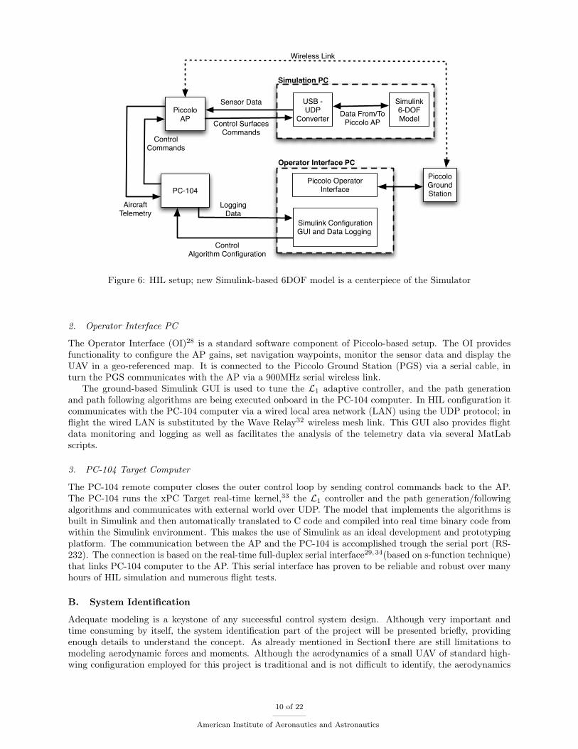
The Avionics of the RASCAL UAV consist of four major functional groups that are shown in Figure 8: (i)a high-bandwidth Persistent Systems WaveRelay wireless mesh router32 that provides communication withthe ground based control PC, (ii) a PC-104 computer that executes the control algorithm and communicateswith the AP, (iii) a Microbotics digital Servo Switch/Controller (SSC)38 that allows for multiple sourcesof servo control, and (iv) the Piccolo Plus AP that implements the inner-loop stabilization and referencefollowing. Most of these components except the digital multiplexor comprise the regular instrumentation ofthe RFTPS setup described in Ref.30.

The SSC was included in the avionics to allow for a pre-programmed single or multiple control surfacefailures; the CSF setup is configured on the ground before each flight but enabled on-demand from the second

11 of 22


RF Modem

Piccolo GCS

Seria

l 1

GCSGPS

Barometer

Independent RC Pilot Console

Operator Interface in a

PCPiccolo Pilot

Console

Wireless Mesh

Control PC

Data Log, Display &

Cong

SimulinkRTWModel

PC-104

RC Rx

AutopilotGPSIMU

Air Data

Seria

l

RF Modem

PWM

Piccolo Plus AP

Wireless Mesh

SwitchLogic Se

rial

PWM

OUT

Digital Switch

PWM

1

PWM

2PWMLine

Select

Cont

rol S

urfa

ces

and

Engi

ne A

ctua

tors

SIG Rascal UAVFailure Mode

UDP

Figure 8: Flight test architecture; integrating digital multiplexer allows for multiple sources of control

pilot console during the flight. This SSC is a highly configurable, multiplexing switch that allows the dynamicselection from three different sources of signals to pass-trough to the control surface actuators. These sourcesare: (i) asynchronous serial communication packets from the PC-104 computer used to generate the failure;(ii) the signals from a conventional RC receiver that is used as a fail-safe mechanism in case the AP fails tostabilize the UAV; and (ii) the PWM signals from the nominal AP to the control surfaces. This architectureallows the user a complete flexibility in defining the nature of the failure. This failure may be configuredto be either one or multiple surfaces and be either a hardover, a neutral position or an oscillating failure asdescribed in Section I.

Another addition to the RFTPS (not shown in Figure 8 for the sake of clarity) is a set of CMOS solidstate video cameras used to record digital video of the simulated CSF; these cameras (Figure 9) are mountedon the airplane so that they continuously observe the control surfaces involved in the experiment. Thefootage produced by these cameras is recovered for further after-flight data analysis.

The airframe utilized as a UAV is one employed by many universities and government labs for research,the Sig Rascal 110, shown in Figure 10. The airframe has a 2.8 m wing span, uses a 26 cm3 gas engine, and atake-off weight of about 10 kg, including 1500 cm3 of gas and enough battery power to provide 120 minutesof flight time. The Rascal can be purchased in an Almost-Ready-to-Fly (ARF) form, making it an extremelycost-effective way to prototype new flight-control systems. The airframe has ample cabin room for the PiccoloAP, the desired computing hardware, sensors, and batteries to provide power to all the avionics.

IV. Control Surfaces Failure Matrix and HIL Results

This section presents the main results obtained with the new HIL simulator described in Section III.A.Thesimulations demonstrate that, if there is enough control authority left, the L1 adaptive augmentation allowsfor safe recovery from the failure with guaranteed transient performance, while the remaining control author-ity may be used to track the turn rate reference commands. The simulations provide also useful informationabout the maximum level of CSF severity that the inner-loop controller is able to compensate for, and thecontrol authority left to control the UAV for every particular failure or combination of failures. Finally,for the case of path following, it is shown that the control algorithm with L1 augmentation introduced inSection II is able to stabilize and steer the UAV along the path in the presence of control surface failures,significantly improving performance of the nominal non-augmented control system.

12 of 22


Figure 9: Videocameras used to record the control surface “failures”

Figure 10: SIG Rascal 110 research aircraft

13 of 22


A. Development of CSF matrix

The proposed failure matrix is built around 8 control surfaces available for independent control of the NPSUAV. As explained in Section III, both HIL and flight test setups offer a great degree of flexibility, allowingone to introduce different single and multiple CSFs. In this paper, as an initial development stage of theproject, only single aileron failures, single rudder failures, and combined aileron/rudder failures have beenconsidered (see Table 1).

Eng. L Elev. R Elev. L Ail. R Ail. Rudd. L Flap R FlapSim HIL Sim HIL Sim HIL

Eng.L Elev.R Elev.L Ail. < 6 < 4

R Ail. < 6 < 4

Rudd.< 6 < 6 < 10

< 4 < 4

L FlapR Flap

Table 1: Simulation and HIL CSF Results

B. HIL Results

The first step consisted of running simulations where the inner-loop controller was tasked to track constantturn rate commands (of different amplitudes) in the presence of the control surface failures considered in thefailure matrix in the previous section. These simulations provided valuable information about the maximumlevel of failure severity that the inner-loop controller can compensate for with and without L1-augmentation,as well as the remaining control authority for every particular failure.

The results showed that the nominal non-augmented autopilot is not able to track the reference signal inthe presence of failures, whereas the L1-augmented inner-loop adapts to provide good tracking performancewith desired recovery transient. Cumulative tracking errors and control efforts were used as metrics toevaluate the performance of the inner-loop in recovering from the control surface failure, while the lateraland normal accelerations provided information about the structural stress on the platform and the quality ofthe recovery transient. Results were obtained for 0 rad

s , 0.05 rads , 0.10 rad

s , and 0.20 rads turn rate commands.

During the second step, and motivated by challenging mission scenarios such as safe landing in thepresence of control surface and/or engine failures, the complete path following control algorithm was testedin the HIL simulator in order to evaluate the performance of the closed-loop system when affected by failures.Figures 11 and 12 show one of the results of these HIL simulations. Particularly, the CSF considered here isa 3 deg left aileron hardover. As it can be seen in Figure 11, the path following control algorithm withoutL1 adaptive augmentation is not able to recover from the failure and track the desired path. Figure 11bshows that, in the presence of the failure, the autopilot itself is not able to track the reference commandcoming from the outer-loop algorithm and we lose control of the UAV. Instead, if the autopilot is augmentedwith the L1 adaptive controller, the UAV is able to recover from the failure and the path following controlsystem uses the remaining control authority to steer the UAV along the path, as shown in Figures 12aand 12b. In particular, Figure 12b shows how the L1 adaptive controller modifies the turn rate commandfrom the outer-loop algorithm so that the actual UAV turn rate tracks it, while Figure 12c shows that boththe right aileron and the rudder help compensate for the left aileron hardover. Figures 12d and 12e show,respectively, the time responses of the state predictor, and the estimation of the uncertainties along withthe resulting L1 control contribution. From these figures, one can easily observe that, for the healthy UAV,the contribution of the L1 augmentation to the command sent to the autopilot is almost zero; whereas, as

14 of 22


soon as the failure appears, the L1 augmentation starts contributing (with desired transient recovery) to thecommand. Figure 12b illustrates also that the remaining control authority in the presence of the aileronfailure is not enough to track outer-loop commands greater than +0.05 m

s . Then, when the outer-loopcommands such a reference, this limitation leads to saturation of the L1 adaptive controller, as it can beseen in Figure 12e. In any case, the path following with L1 augmentation keeps the closed-loop controlsystem stable all the time.

(a) Path tracking (2D projection). (b) Commanded yaw rate rc(t) tracking.

Figure 11: HIL. Path following without L1 adaptive augmentation.

We note that, in this approach, the autopilot does not know that the failure occurred, and thus there isno need for failure detection and isolation (FDI) in order to compensate for the failure: the L1 augmentedinner-loop adapts to the new dynamics of the plant, and the UAV can be steered along the path using theremaining control authority. We also note that, in order to guarantee, for example, safe landing capabilitiesin the presence of failures, information about the remaining control authority should be supplied to thetrajectory optimization algorithm in order to generate a new path for safe landing of the impaired airplane.However, this remains an open problem, and further theoretical and experimental study should be conductedon the identification and management of the remaining control authority.

V. Flight Test Results

In this section, sample results from a series of flight experiments implementing real CSF are shownproviding some insight primarily into the recovery capabilities of real system with L1 augmented pathfollowing algorithm. It also serves the auxiliary function of proving the correctness of the concept adheredto the project through analyzing the consistency of principal results obtained in the control system designand pure software simulation, HIL simulation and flight test stages of the programm.

A. Flight Testing Procedure

The flight testing was performed over a span of several days in July 2008, in Camp Roberts CA. Flight testsetup is identical to the one presented in HIL section except that sensor measurements are not simulated.In the first series of flights, the parameters of the PID gains for the nominal AP, path following kinematiccontroller and L1 augmentation loop were those obtained in HIL simulation. A small tuning of L1 aug-mentation loop decreasing the bandwidth of both estimator and low pass filter was initially performed totest more conservative and therefore less aggressive augmentation. Later on, when nominal performance ofthe healthy system in path following mode with L1 controller enabled was verified, the original parameterswere applied. More details on tuning the path following controller and the L1 adaptive augmentation can

15 of 22


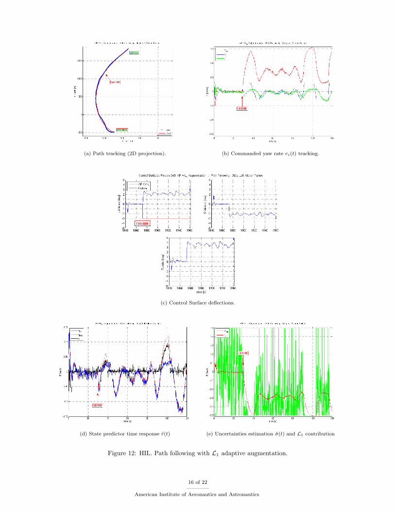
(a) Path tracking (2D projection). (b) Commanded yaw rate rc(t) tracking.

(c) Control Surface deflections.

(d) State predictor time response r(t) (e) Uncertainties estimation σ(t) and L1 contribution

Figure 12: HIL. Path following with L1 adaptive augmentation.

16 of 22


be found in Ref.25 .Overall, two series of CSF test were performed: first, a left aileron hardover; and second, a rudder

hardover. After every takeoff, the UAV was trimmed in wings level flight, which allowed us to capture thetrim positions for all the control surfaces. Then, these trim deflections for ailerons and rudder were usedas a reference level to introduce the failures and to evaluate the severity of the failure. It is also necessaryto note that the CSF was introduced with a small delay (usually not more that 2-3 seconds) after the pathfollowing algorithm was engaged. This is due to the fact that the confirmation of the CSF command wassent from the secondary pilot console that triggered the digital switch onboard (see Fig. 8).

B. Testing Ailerons and Rudder Channels

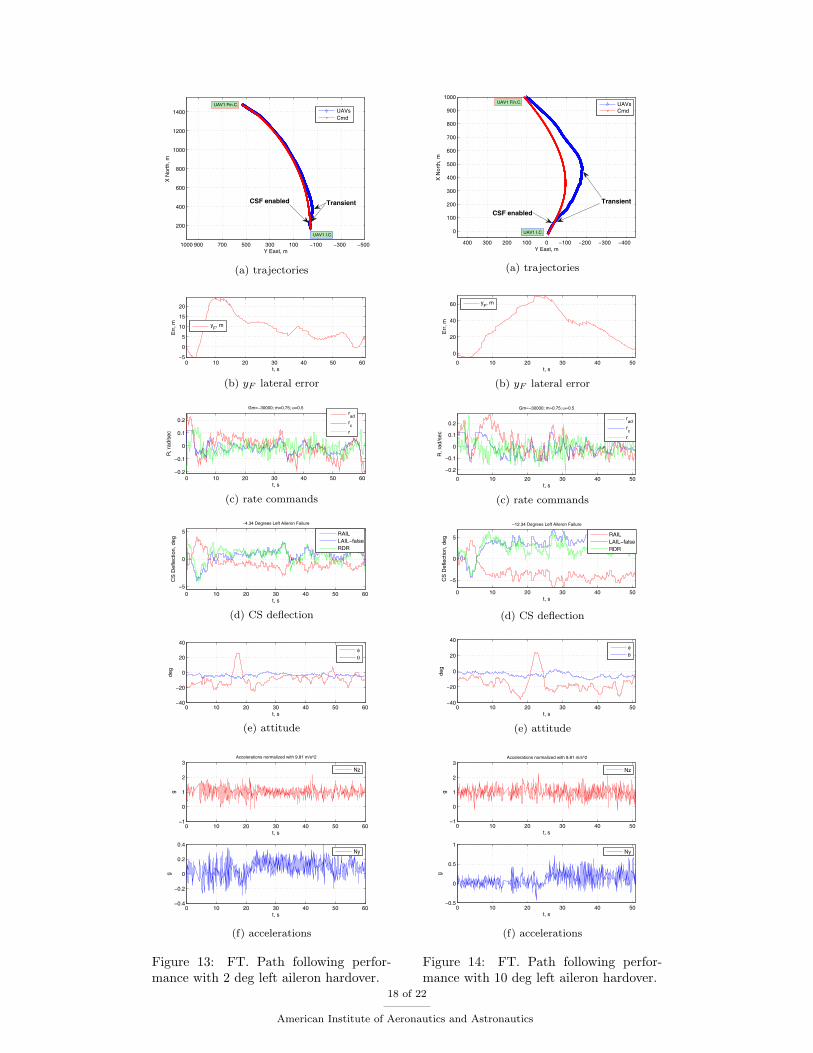
The first set of figures illustrates the performance of the system with two levels of left aileron failure at−2 deg and −10 deg (trim value for the left aileron was captured at −2.34 deg). Although there were 6trials performed starting at 0 deg and ending at −12 deg of a left aileron hardover, these two cases providebetter inside on the L1 contribution. The −12 deg of a left aileron hardover resulting in −14.34 deg of totalaileron deflection was a marginal case when the closed-loop system was marginally stable. Therefore, theprevious step was chosen as a margin for the L1 controller recovering capability.

Analysis of the −2 deg case shows that even such small deflection pushes UAV away to the right from thecommanded trajectory (while the generated path turns left, Fig. 13a) resulting in almost 25 meters lateralmiss distance, see Fig. 13b). Initial rate transient (Fig. 13c) is almost negligible, although its integral effectis better seen on the trajectory plot; the L1 is ON and r response follows rad command perfectly well. Theintroduced CSF results in the UAV taking next 20 seconds to converge to 5 meters lateral error boundary.The attitude angles (Fig. 13e) show that the UAV is capable to keep banking to the left (mean value at−10) for the entire duration of the experiment, therefore following the trajectory. In particular, rates plotconfirms that the L1 adaptive controller (rad) modifies the turn rate command from the outer-loop (rc)algorithm so that the actual UAV turn rate (r) tracks it, while the CS deflection plot (Fig. 13d) shows thatboth the right aileron and the rudder compensate for the left aileron hardover. History of the control surfacedeflection confirms that the AP continues sending commands to the left aileron since it is not aware of thefailure. With the total deflection of failed aileron at −4.34 deg the control algorithm forces the inner-loopof nominal AP to deflect both the symmetric aileron and the rudder, that significantly helps in tracking thegiven path. The plots of lateral and normal accelerations (Fig. 13f) show that, while in failure mode, theaccelerations are well maintained, and therefore the UAV does not experience any excessive load providingreasonable ride quality.

The results of the −10 deg left aileron failure (Figure 14) are almost identical to the previous case. Theerrors and the compensating control efforts are increased due to the increased severity of the failure. Theanalysis shows uniform degradation of tracking performance that allows for easy prediction of the performancebounds, that is extremely important for such a challenging situation. Overall, the controller recovers fromthe severe failure taking longer time (30 seconds) to converge to the same 5 meters lateral error boundary.

Experimenting with the rudder failures confirmed its significant control authority in the lateral channel.As a result much smaller range of rudder failure was achieved. The following set of figures (Fig. 15) illustratesthe performance of the L1 adaptive controller. Analysis of even 0 deg rudder failure shows significant lossof controllability: the lateral error (Fig. 15b) rises up to 35 m, it takes longer time to recover from thetransient (30 s) to the same 5 meters lateral error boundary. The fact that the rate response r (Fig. 15c) is90 deg off-phase from the commanded rad (AP still commands turn rate through rudder, but only aileronsare available) for both cases of failure confirms that the L1 controller automatically re-adjusts the turn ratecommand to the fixed, but unknown, mixing of the aileron to rudder channels. The case of −2 deg rudderfailure shows the marginal performance of the augmented system in recovering the path following.

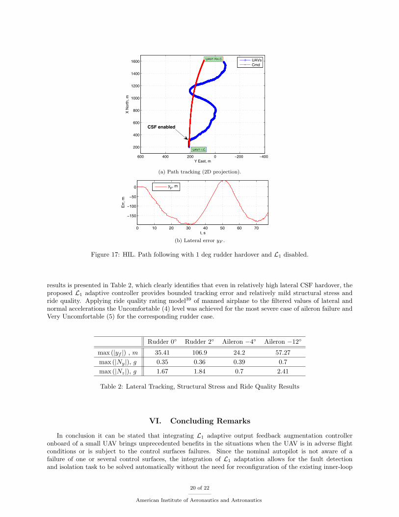
The fact that the nominal AP cannot track a given path without L1 augmentation is explicitly illustratednext in Figure 17a where system response to 1 deg rudder failure without L1 is shown. Figure 17b showsdynamics of lateral error with the rudder fixed at 1. The non-stabilizing divergence of the lateral errorprovides the most illustrative proof of that.

Initial evaluation of the L1 adaptation performance in recovering the UAV in the path following modeunder the CSF was based on the following two representative metrics. The first one reflects the lateraltracking error by analyzing the maximum lateral deviation from a commanded path – max (|yf |). Thesecond one represents the desire to obtain sufficient indication of structural stress and ride quality bestreflected by the maximum lateral and normal accelerations – max (|Ny|), max (|Nz|). Analysis of the obtained

17 of 22


−500−300−1001003005007009001000

200

400

600

800

1000

1200

1400

UAV1 I.C.

UAV1 Fin.C.

Y East, m

X N

orth

, m

UAVsCmd

TransientCSF enabled

(a) trajectories

0 10 20 30 40 50 60−5

0

5

10

15

20

Err

, m

t, s

yF, m

(b) yF lateral error

0 10 20 30 40 50 60−0.2

−0.1

0

0.1

0.2

R, r

ad/s

ec

t, s

Gm=−30000; m=0.75; ω=0.5

rad

rc

r

(c) rate commands

0 10 20 30 40 50 60−5

0

5

CS

Def

lect

ion,

deg

t, s

−4.34 Degrees Left Aileron Failure

RAILLAIL−falseRDR

(d) CS deflection

0 10 20 30 40 50 60−40

−20

0

20

40

t, s

deg

φθ

(e) attitude

0 10 20 30 40 50 60−1

0

1

2

3

t, s

g

Accelerations normalized with 9.81 m/s^2

Nz

0 10 20 30 40 50 60−0.4

−0.2

0

0.2

0.4

t, s

g

Ny

(f) accelerations

Figure 13: FT. Path following perfor-mance with 2 deg left aileron hardover.

−400−300−200−1000100200300400

0

100

200

300

400

500

600

700

800

900

1000

UAV1 I.C.

UAV1 Fin.C.

Y East, m

X N

orth

, m

UAVsCmd

CSF enabled

Transient

(a) trajectories

0 10 20 30 40 50

0

20

40

60

Err

, m

t, s

y

F, m

(b) yF lateral error

0 10 20 30 40 50

−0.2

−0.1

0

0.1

0.2

R, r

ad/s

ec

t, s

Gm=−30000; m=0.75; ω=0.5

rad

rc

r

(c) rate commands

0 10 20 30 40 50

−5

0

5

CS

Def

lect

ion,

deg

t, s

−12.34 Degrees Left Aileron Failure

RAILLAIL−falseRDR

(d) CS deflection

0 10 20 30 40 50−40

−20

0

20

40

t, s

deg

φθ

(e) attitude

0 10 20 30 40 50−1

0

1

2

3

t, s

g

Accelerations normalized with 9.81 m/s^2

Nz

0 10 20 30 40 50−0.5

0

0.5

1

t, s

g

Ny

(f) accelerations

Figure 14: FT. Path following perfor-mance with 10 deg left aileron hardover.

18 of 22


−700−600−500−400−300−200−10001002003000

200

400

600

800

1000

1200

UAV1 I.C.

UAV1 Fin.C.

Y East, m

X N

orth

, m

UAVsCmd

CSF enabled

(a) trajectories

0 10 20 30 40 50 600

10

20

30

Err

, m

t, s

y

F, m

(b) yf lateral error

0 10 20 30 40 50 60

−0.2

−0.1

0

0.1

0.2

R, r

ad/s

ec

t, s

Gm=−30000; m=0.75; ω=0.5

rad

rc

r

(c) rate commands

0 10 20 30 40 50 60

−4

−2

0

2

4

CS

Def

lect

ion,

deg

t, s

0 Degrees Rudder Failure

RAILLAILRDR−false

(d) CS deflection

0 10 20 30 40 50 60−30

−20

−10

0

10

t,s

degr

ees

φθ

(e) attitude

0 10 20 30 40 50 600

0.5

1

1.5

2

t,s

g

Nz

0 10 20 30 40 50 60−0.4

−0.2

0

0.2

0.4

t,s

g

Ny

(f) accelerations

Figure 15: FT. Path following perfor-mance with 0 deg rudder hardover.

−200−1000100200300400

200

400

600

800

1000

1200

1400

UAV1 I.C.

UAV1 Fin.C.

Y East, m

X N

orth

, m

UAVsCmd

CSF enabled

(a) trajectories

0 10 20 30 40 50 60−100

−50

0

50

Err

, m

t, s

y

F, m

(b) yf lateral error

0 10 20 30 40 50 60

−0.2

−0.1

0

0.1

0.2

0.3

R, r

ad/s

ec

t, s

Gm=−30000; m=0.75; ω=0.5

rad

rc

r

(c) rate commands

0 10 20 30 40 50 60

−4

−2

0

2

4

6

CS

Def

lect

ion,

deg

t, s

−2 Degrees Rudder Failure

RAILLAILRDR−false

(d) CS deflection

0 10 20 30 40 50 60−60

−40

−20

0

20

40

t,s

degr

ees

φθ

(e) attitude

0 10 20 30 40 50 600

0.5

1

1.5

2

t,s

g

Nz

0 10 20 30 40 50 60−0.1

0

0.1

0.2

0.3

0.4

t,s

g

Ny

(f) accelerations

Figure 16: FT. Path following perfor-mance with 2 deg rudder hardover.

19 of 22


−400−2000200400600

200

400

600

800

1000

1200

1400

1600

UAV1 I.C.

UAV1 Fin.C.

Y East, m

X N

orth

, m

UAVsCmd

CSF enabled

(a) Path tracking (2D projection).

0 10 20 30 40 50 60 70

−150

−100

−50

0

Err

, m

t, s

y

F, m

(b) Lateral error yF .

Figure 17: HIL. Path following with 1 deg rudder hardover and L1 disabled.

results is presented in Table 2, which clearly identifies that even in relatively high lateral CSF hardover, theproposed L1 adaptive controller provides bounded tracking error and relatively mild structural stress andride quality. Applying ride quality rating model39 of manned airplane to the filtered values of lateral andnormal accelerations the Uncomfortable (4) level was achieved for the most severe case of aileron failure andVery Uncomfortable (5) for the corresponding rudder case.

Rudder 0 Rudder 2 Aileron −4 Aileron −12

max (|yf |) , m 35.41 106.9 24.2 57.27max (|Ny|), g 0.35 0.36 0.39 0.7max (|Nz|), g 1.67 1.84 0.7 2.41

Table 2: Lateral Tracking, Structural Stress and Ride Quality Results

VI. Concluding Remarks

In conclusion it can be stated that integrating L1 adaptive output feedback augmentation controlleronboard of a small UAV brings unprecedented benefits in the situations when the UAV is in adverse flightconditions or is subject to the control surfaces failures. Since the nominal autopilot is not aware of afailure of one or several control surfaces, the integration of L1 adaptation allows for the fault detectionand isolation task to be solved automatically without the need for reconfiguration of the existing inner-loop

20 of 22


control structure of the nominal AP. As a result, the L1 augmented controller readjusts the control inputthat stabilizes the impaired airplane and uses the remaining control authority to steer the airplane along theredefined path. Therefore, integrating L1 adaptation onboard increases the fault tolerance of the system.

Initial development of the control quality metrics resulted in establishing a set of qualitative measuresthat were verified experimentally in HIL and flight testing. It was experimentally shown in extensive HILand flight testing that L1 augmented system exhibits uniform degradation of tracking performance in thepresence of increasing severity of the CS failure. Theoretical and experimental study of the remaining controlauthority and robustness is in progress.

On the experimental side of the project several major milestones were achieved including development ofa new HIL simulating capability for a Piccolo Plus AP that allows for advanced modeling of non-conventionalairplane configurations and aerodynamics using convenience of Simulink development environment and con-trol design toolboxes. Furthermore, new modification of the RFTPS was developed providing a rigorouscapability of flight testing of the airplanes with complex failures of control surfaces in various flight regimesand configurations.

VII. Acknowledgments

This work was sponsored in part by NASA Grants NNX08AB97A, NNX08AC81A, and NNL08AA12I,and Hellenic Air Force Research Grant (KAE 0482/EF11-410).

References

1Belcastro, C., Khong, T., Shin, J., Kwatny, H., Chang, B., and Balas, G., “Uncertainty Modeling for Robustness Analysisof Aircraft Control Upset Prevention and Recovery Systems,” .

2Foster, J., Cunningham, K., Fremaux, C., Shah, G., Stewart, E., Rivers, R., Wilborn, J., and Gato, W., “DynamicsModeling and Simulation of Large Transport Airplanes in Upset Conditions,” 2005 AIAA Guidance, Navigation, and ControlConference and Exhibit , 2005, pp. 1–13.

3Nguyen, N., Krishnakumar, K., Kaneshige, J., and Nespeca, P., “Dynamics and Adaptive Control for Stability Recoveryof Damaged Asymmetric Aircraft,” AIAA Guidance, Navigation, and Control Conference Proceedings, 2006.

4C., N. T. S. B., “in-flight Separation of Vertical Stabilizer American Airline Flight 587 Airbus Industrie A300-605RN14053 Belle Harbor, New York, November 12, 2001,” Tech. rep., NTSB, 2004.

5Board, N. T. S., “Loss of Control and Impact with Pacific Ocean Alaska Airlines Flight 261 McDonnel Douglas MD-83,N963AS about 2.7 Miles North of Anacpa Island, CA, Jan. 31, 2000,” Tech. rep., 2002, NTSB/AAR-02/01.

6Board, N. T. S., “Loss of Pitch Control During Takeoff Air Midwest 5481 Raytheon (Beechcraft) 1900D, N233YV,Charlotte, NC Jan. 8, 2003,” Tech. rep., 2004, NTSB/AAR-04/01.

7Jordan, T., Langford, W., and Hill, J., “Airborne Subscale Transport Aircraft Research Testbed-Aircraft Model Devel-opment,” AIAA Guidance, Navigation, and Control Conference and Exhibit , pp. 2005–6432.

8Croft, J., “Refuse-to-crash: NASA tackles loss of control.” Aerosp Am, Vol. 41, No. 3, 2003, pp. 42–5.9Cao, C. and Hovakimyan, N., “Guaranteed Transient Performance with L1 Adaptive Controller for Systems with Unknown

Time-Varying Parameters: Part I,” New York, NY, July 2007, pp. 3925–3930.10Cao, C. and Hovakimyan, N., “Stability Margins of L1 Adaptive Controller: Part II,” New York, NY, July 2007, pp.

3931–3936.11Klein, V. and Morelli, E., Aircraft System identification: Theory and Practise, 2006.12Morelli, E. and Klein, V., “Application of System Identification to Aircraft at NASA Langley Research Center,” Journal

of Aircraft , Vol. 42, No. 1, 2005, pp. 12–25.13Morton, S., Forsythe, J., McDaniel, D., Bergeron, K., Cummings, R., Goertz, S., Seidel, J., and Squires, K., “High

Resolution Simulation of Full Aircraft Control at Flight Reynolds Numbers,” DoD High Performance Computing ModernizationProgram Users Group Conference, 2007 , 2007, pp. 41–47.

14Milam, M., Mushambi, K., and Murray, R., “A new computational approach to real-time trajectory generation forconstrained mechanical systems,” Decision and Control, 2000. Proceedings of the 39th IEEE Conference on, Vol. 1, 2000.

15Milam, M., Franz, R., and Murray, R., “Real-time constrained trajectory generation applied to a flight control experi-ment,” 2002 IFAC World Congress, Barcelona, Spain, 2002.

16Frazzoli, E., Dahleh, M., and Feron, E., “Real-time motion planning for agile autonomous vehicles,” J GUID CONTROLDYN , Vol. 25, No. 1, 2002, pp. 116–129.

17Yakimenko, O., “Direct Method for Rapid Prototyping of Near-Optimal Aircraft Trajectories,” AIAA Journal of Guid-ance, Control, & Dynamics, Vol. 23, No. 5, 2000, pp. 865–875.

18Dobrokhodov, V. and Yakimenko, O., “Synthesis of Trajectorial Control Algorithms at the Stage of Rendezvous ofan Airplane with a Maneuvering Object,” Journal of Computer and Systems Sciences International , Vol. 38, No. 2, 1999,pp. 262–277.

19Kaminer, I., Yakimenko, O., Dobrokhodov, V., Lizarraga, M., and Pascoal, A., “Cooperative control of small UAVs fornaval applications,” Decision and Control, 2004. CDC. 43rd IEEE Conference on, Vol. 1, 2004.

21 of 22


20Cao, C. and Hovakimyan, N., “Design and Analysis of a Novel L1 Adaptive Control Architecture, Part I: Control Signaland Asymptotic Stability,” Minneapolis, MN, June 2006, pp. 3397–3402.

21Cao, C. and Hovakimyan, N., “Design and Analysis of a Novel L1 Adaptive Control Architecture, Part II: GuaranteedTransient Performance,” Minneapolis, MN, June 2006, pp. 3403–3408.

22Cao, C. and Hovakimyan, N., “L1 Adaptive Output Feedback Controller for Systems with Time-varying UnknownParameters and Bounded Disturbances,” New York, NY, July 2007, pp. 486–491.

23Cao, C. and Hovakimyan, N., “L1 Adaptive Output Feedback Controller for Systems of Unknown Dimension,” IEEETransactions on Automatic Control , Vol. 53, No. 3, April 2008, pp. 815–821.

24Kaminer, I., Yakimenko, O., Pascoal, A., and Ghabcheloo, R., “Path Generation, Path Following and CoordinatedControl for Time Critical Missions of Multiple UAVs,” American Control Conference, June 2006, pp. 4906 – 4913.

25Kaminer, I., Pascoal, A., Xargay, E., Cao, C., Hovakimyan, N., and Dobrokhodov, V., “3D Path Following for SmallUAVs using Commercial Autopilots augmented by L1 Adaptive Control,” Submitted to Journal of Guidance, Control andDynamics.

26Pomet, J. B. and Praly, L., “Adaptive Nonlinear Regulation: Estimation from the Lyapunov Equation,” Vol. 37(6), June1992, pp. 729–740.

27The Mathworks, Natick, MA, Simulink User’s Guide, 2008.28Vaglienti, B., Hoag, R., and Niculescu, M., Piccolo System Documentation, Cloud Cap Technologies, April 2005,

http://www.cloudcaptech.com.29Dobrokhodov, V. and Lizarraga, M., “Developing Serial Communication Interfaces for Rapid Prototyping of Navigation

and Control Tasks,” AIAA, Vol. 6099, 2005, pp. 2005.30Dobrokhodov, V., Yakimenko, O., Jones, K., Kaminer, I., Bourakov, E., Kitsios, I., and Lizarraga, M., “New Generation

of Rapid Flight Test Prototyping System for Small Unmanned Air Vehicles,” AIAA Modeling and Simulation TechnologiesConference Proceedings, 2007.

31Vaglienti, B., Communications for the Piccolo avionics, Cloud Cap Technologies, September 2006,http://www.cloudcaptech.com.

32Persistent Systems, The Wave RelayTM Quad Radio Router , August 2008, http://www.persistentsystems.com.33The Mathworks, Natick, MA, xPC Target User’s Guide, 2008.34Lizarraga, M. I., Autonomous Landing System for a UAV , Master’s thesis, Naval Postgraduate School, Monterey, CA,

USA., March 2004.35Desktop Aeronautics, P.O. Box 20384, Stanford CA 94309, LinAir User’s Guide, 2005.36Statnikov, R., Multicriteria Design: Optimization and Identification, Kluwer Academic Publishers, 1999.37Dobrokhodov, V. and Statnikov, R., “Multi-Criteria Identification of a Controllable Descending System,” Computational

Intelligence in Multicriteria Decision Making, IEEE Symposium on, 2007, pp. 212–219.38Microbotics, Inc, Microbotics Inc. 28 Research Drive, Suite G,Hampton, VA 23666-1364, Servo Switch/Controller Users

Manual , August 2008, http://www.microboticsinc.com.39Powers, B. G., “Analytical Study of Ride Smoothing Benefits of Control System Configurations Optimized for Pilot

Handling Quaities,” Technical paper, NASA Dryden Flight Research Center, Edwards, CA, NASA DFRC, February 1978.

22 of 22


flight validation of metrics driven l1 adaptive control

Documents