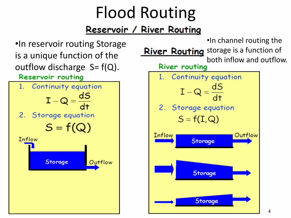
Flood Routing

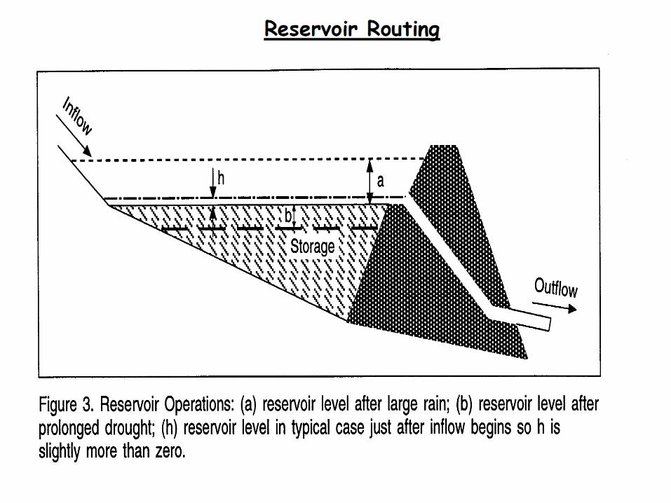
•In channel routing the storage is a function of both inflow and outflow.

•In reservoir routing Storage is a unique function of the outflow discharge S= f(Q).

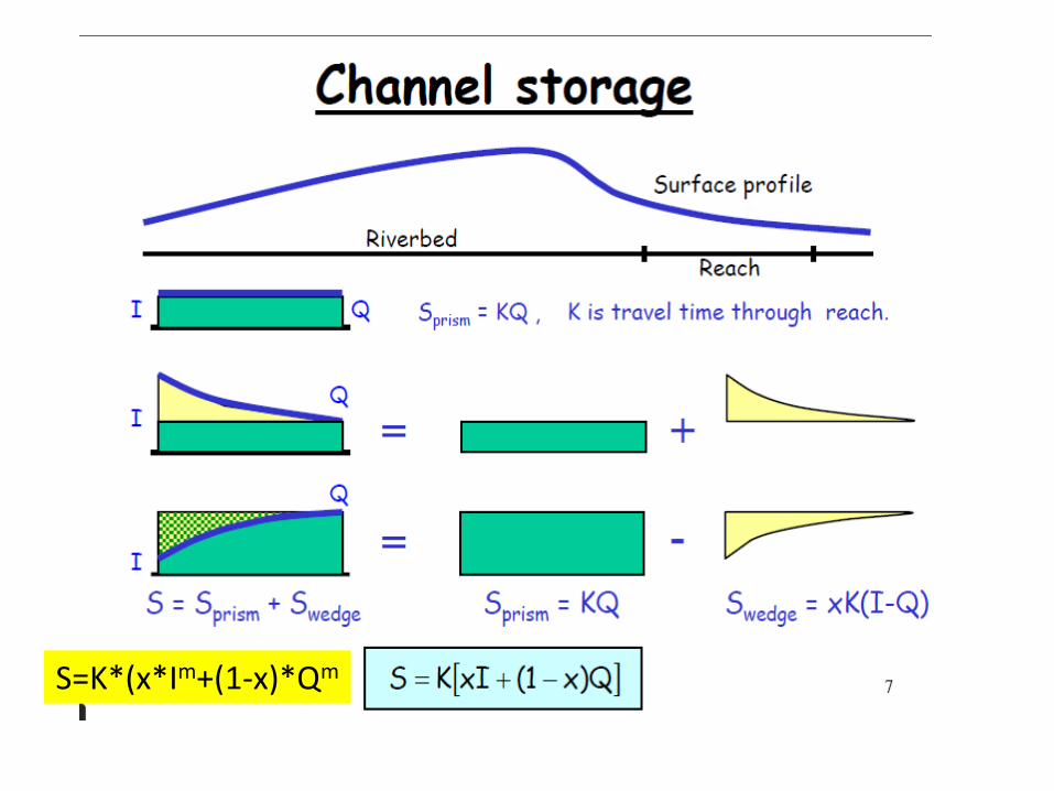
S=K*(x*Im+(1-x)*Qm

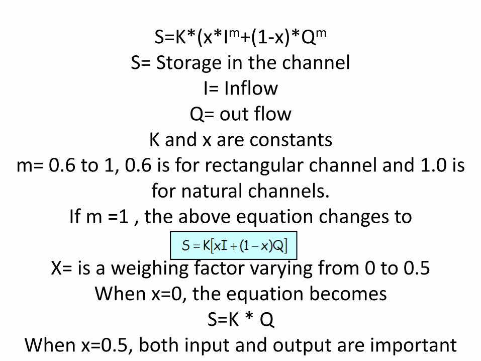
S=K*(x*Im+(1-x)*Qm

S= Storage in the channel I= Inflow

Q= out flow

K and x are constants m= 0.6 to 1, 0.6 is for rectangular channel and 1.0 is

for natural channels. If m =1 , the above equation changes to

X= is a weighing factor varying from 0 to 0.5

When x=0, the equation becomes S=K * Q

When x=0.5, both input and output are important

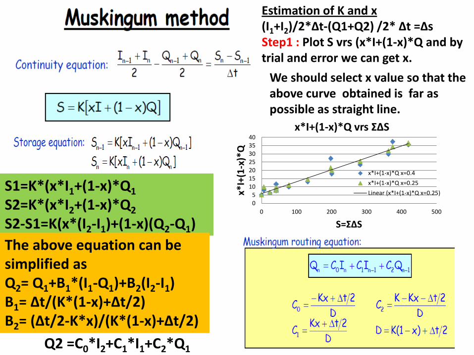
Estimation of K and x (I1+I2)/2*∆t-(Q1+Q2) /2* ∆t =∆s Step1 : Plot S vrs (x*I+(1-x)*Q and by trial and error we can get x.

We should select x value so that the above curve obtained is far as possible as straight line.

0

5

10

15

20

25

30

35

40

0 100 200 300 400 500

x*I+

(1-x

)*Q

S=Σ∆S

x*I+(1-x)*Q vrs Σ∆S

x*I+(1-x)*Q x=0.4

x*I+(1-x)*Q x=0.25

Linear (x*I+(1-x)*Q x=0.25)S1=K*(x*I1+(1-x)*Q1 S2=K*(x*I2+(1-x)*Q2 S2-S1=K(x*(I2-I1)+(1-x)(Q2-Q1)

The above equation can be simplified as Q2= Q1+B1*(I1-Q1)+B2(I2-I1) B1= ∆t/(K*(1-x)+∆t/2) B2= (∆t/2-K*x)/(K*(1-x)+∆t/2)

Q2 =C0*I2+C1*I1+C2*Q1

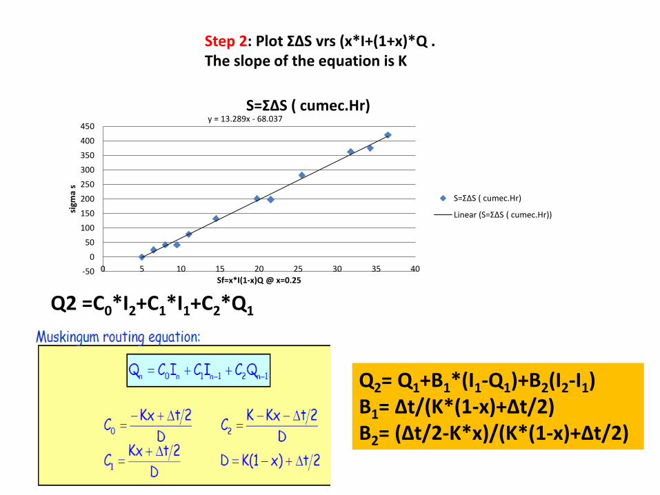
y = 13.289x - 68.037

-50

0

50

100

150

200

250

300

350

400

450

0 5 10 15 20 25 30 35 40

sigm

a s

Sf=x*I(1-x)Q @ x=0.25

S=Σ∆S ( cumec.Hr)

S=Σ∆S ( cumec.Hr)

Linear (S=Σ∆S ( cumec.Hr))

Step 2: Plot Σ∆S vrs (x*I+(1+x)*Q . The slope of the equation is K

Q2 =C0*I2+C1*I1+C2*Q1

Q2= Q1+B1*(I1-Q1)+B2(I2-I1) B1= ∆t/(K*(1-x)+∆t/2) B2= (∆t/2-K*x)/(K*(1-x)+∆t/2)

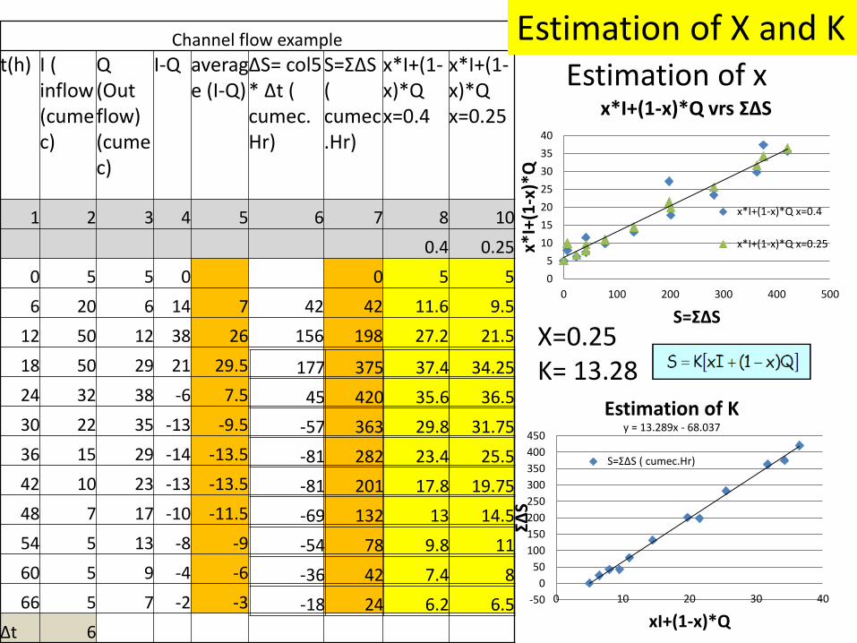
Channel flow example

t(h) I ( inflow (cumec)

Q (Out flow) (cumec)

I-Q average (I-Q)

∆S= col5 * ∆t ( cumec.Hr)

S=Σ∆S ( cumec.Hr)

x*I+(1-x)*Q x=0.4

x*I+(1-x)*Q x=0.25

1 2 3 4 5 6 7 8 10

0.4 0.25

0 5 5 0 0 5 5

6 20 6 14 7 42 42 11.6 9.5

12 50 12 38 26 156 198 27.2 21.5

18 50 29 21 29.5

24 32 38 -6 7.5

30 22 35 -13 -9.5

36 15 29 -14 -13.5

42 10 23 -13 -13.5

48 7 17 -10 -11.5

54 5 13 -8 -9

60 5 9 -4 -6

66 5 7 -2 -3

∆t 6

0

5

10

15

20

25

30

35

40

0 100 200 300 400 500

x*I+

(1-x

)*Q

S=Σ∆S

x*I+(1-x)*Q vrs Σ∆S

x*I+(1-x)*Q x=0.4

x*I+(1-x)*Q x=0.25

Estimation of x

y = 13.289x - 68.037

-50

0

50

100

150

200

250

300

350

400

450

0 10 20 30 40

Σ∆S

xI+(1-x)*Q

Estimation of K

S=Σ∆S ( cumec.Hr)

X=0.25 K= 13.28 177 375 37.4 34.25

45 420 35.6 36.5

-57 363 29.8 31.75

-81 282 23.4 25.5

-81 201 17.8 19.75

-69 132 13 14.5

-54 78 9.8 11

-36 42 7.4 8

-18 24 6.2 6.5

Estimation of X and K

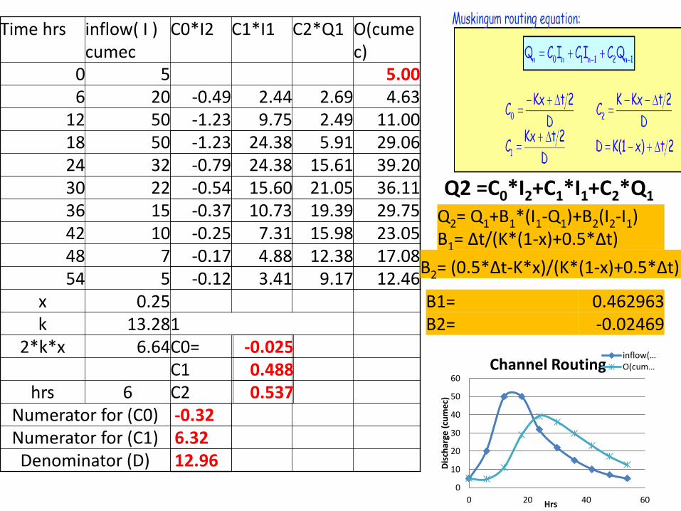
Time hrs inflow( I ) cumec

C0*I2 C1*I1 C2*Q1 O(cumec)

0 5 5.00 6 20 -0.49 2.44 2.69 4.63

12 50 -1.23 9.75 2.49 11.00 18 50 24 32 30 22 36 15 42 10 48 7 54 5

x 0.25 k 13.28 1

2*k*x 6.64 C0= C1

hrs 6 C2 Numerator for (C0) Numerator for (C1) Denominator (D)

-1.23 24.38 5.91 29.06 -0.79 24.38 15.61 39.20 -0.54 15.60 21.05 36.11 -0.37 10.73 19.39 29.75 -0.25 7.31 15.98 23.05 -0.17 4.88 12.38 17.08 -0.12 3.41 9.17 12.46

B1= 0.462963 B2= -0.02469

Q2= Q1+B1*(I1-Q1)+B2(I2-I1) B1= ∆t/(K*(1-x)+0.5*∆t)

B2= (0.5*∆t-K*x)/(K*(1-x)+0.5*∆t)

0

10

20

30

40

50

60

0 20 40 60

Dis

char

ge (

cum

ec)

Hrs

Channel Routing inflow(…O(cum…

Q2 =C0*I2+C1*I1+C2*Q1

-0.32 6.32 12.96

-0.025 0.488 0.537

Modified Pulse Method Goodrich Method

10

Goodrich Method

t

S - S =

2

O + O( -

2

I + I 122121

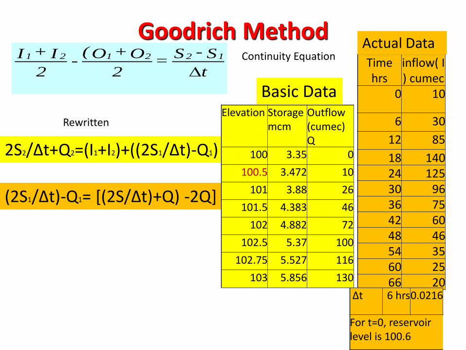
Continuity Equation

Rewritten

2S2/∆t+Q2=(I1+I2)+((2S1/∆t)-Q1)

(2S1/∆t)-Q1= *(2S/∆t)+Q) -2Q]

Elevation Storage mcm

Outflow (cumec) Q

100 3.35 0

100.5 3.472 10

101 3.88 26

101.5 4.383 46

102 4.882 72

102.5 5.37 100

102.75 5.527 116

103 5.856 130

Basic Data

Time hrs

inflow( I ) cumec

0 10

6 30

12 85

18 140 24 125 30 96 36 75 42 60 48 46 54 35 60 25 66 20

Actual Data

∆t 6 hrs 0.0216

For t=0, reservoir level is 100.6

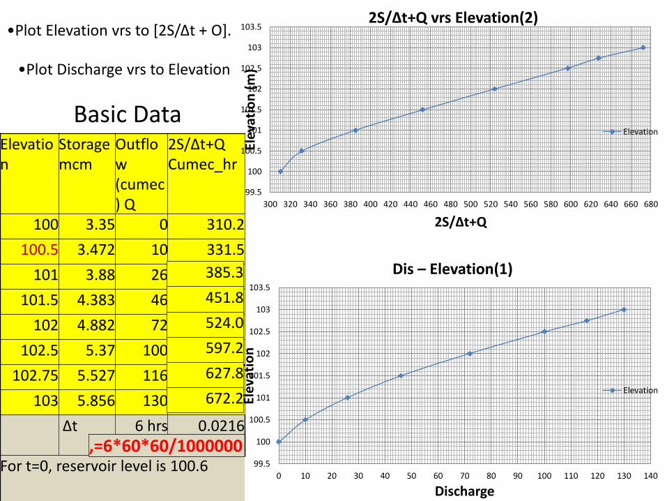
Elevation

Storage mcm

Outflow (cumec) Q

2S/∆t+Q Cumec_hr

100 3.35 0 310.2

100.5 3.472 10 331.5

101 3.88 26

101.5 4.383 46

102 4.882 72

102.5 5.37 100

102.75 5.527 116

103 5.856 130

∆t

6 hrs 0.0216

For t=0, reservoir level is 100.6

Basic Data

99.5

100

100.5

101

101.5

102

102.5

103

103.5

300 320 340 360 380 400 420 440 460 480 500 520 540 560 580 600 620 640 660 680

Elev

atio

n (

m)

2S/∆t+Q

2S/∆t+Q vrs Elevation(2)

Elevation

99.5

100

100.5

101

101.5

102

102.5

103

103.5

0 10 20 30 40 50 60 70 80 90 100 110 120 130 140

Elev

atio

n

Discharge

Dis – Elevation(1)

Elevation

•Plot Elevation vrs to [2S/Δt + O].

•Plot Discharge vrs to Elevation

385.3

451.8

524.0

597.2

627.8

672.2

,=6*60*60/1000000

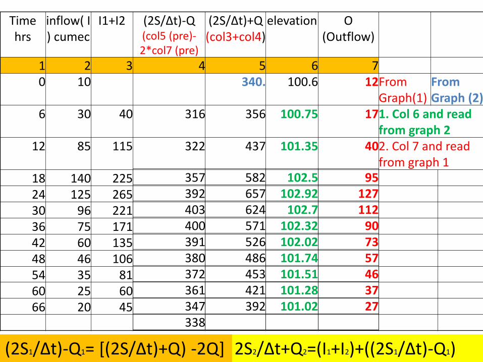
Time hrs

inflow( I ) cumec

I1+I2 (2S/∆t)-Q (col5 (pre)-2*col7 (pre)

(2S/∆t)+Q (col3+col4)

elevation O (Outflow)

1 2 3 4 5 6 7 0 10 340. 100.6 12 From

Graph(1) From Graph (2)

6 30 40 316 356 100.75 17 1. Col 6 and read from graph 2

12 85 115 322 437 101.35 40 2. Col 7 and read from graph 1

18 140 225 24 125 265 30 96 221 36 75 171 42 60 135 48 46 106 54 35 81 60 25 60 66 20 45

357 582 102.5 95 392 657 102.92 127 403 624 102.7 112 400 571 102.32 90 391 526 102.02 73 380 486 101.74 57 372 453 101.51 46 361 421 101.28 37 347 392 101.02 27 338

2S2/∆t+Q2=(I1+I2)+((2S1/∆t)-Q1) (2S1/∆t)-Q1= *(2S/∆t)+Q) -2Q]

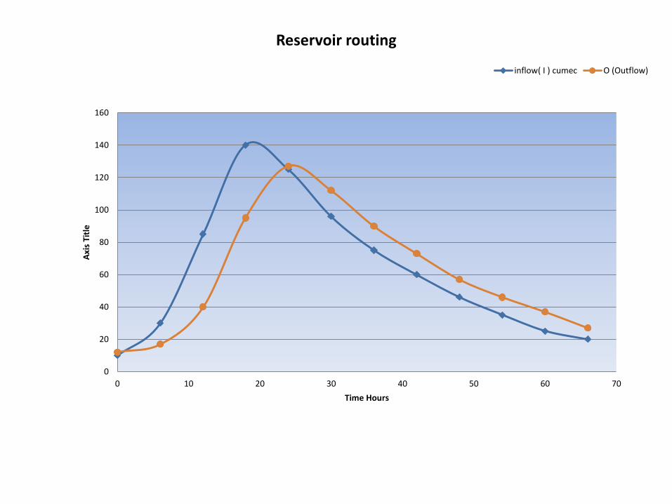
0

20

40

60

80

100

120

140

160

0 10 20 30 40 50 60 70

Axi

s Ti

tle

Time Hours

Reservoir routing

inflow( I ) cumec O (Outflow)

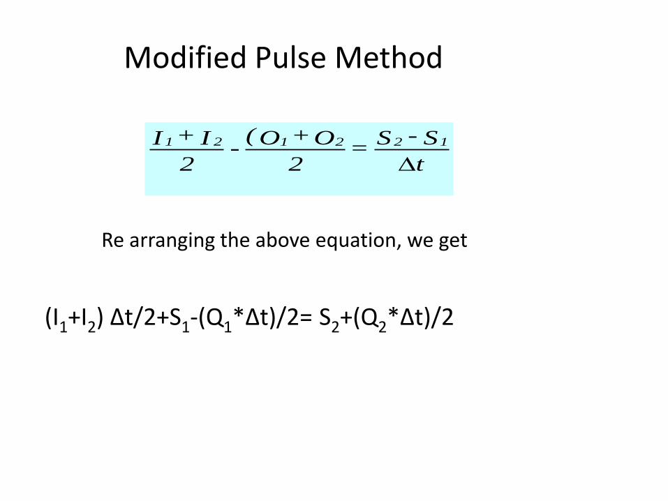
Modified Pulse Method

t

S - S =

2

O + O( -

2

I + I 122121

(I1+I2) Δt/2+S1-(Q1*Δt)/2= S2+(Q2*Δt)/2

Re arranging the above equation, we get