florian strunk - uni-osnabrueck.denbn:de:gbv:... · on motivic spherical bundles florian strunk...
TRANSCRIPT

ON MOTIVIC SPHERICAL BUNDLES
FLORIAN STRUNK
Dissertation
zur
Erlangung des Doktorgrades (Dr. rer. nat.)
des Fachbereichs Mathematik/Informatik
an der Universitat Osnabruck
vorgelegt von
Florian Strunk
aus Lemgo
Institut fur Mathematik
Universitat Osnabruck
Dezember 2012

Contents
Introduction 1
1. Unstable motivic homotopy theory 3
1.1. The unstable motivic homotopy category . . . . . . . . . . . . . . . . 5
1.2. Homotopy sheaves and fiber sequences . . . . . . . . . . . . . . . . . 15
1.3. Mather’s cube theorem and some implications . . . . . . . . . . . . . . 24
2. Stable motivic homotopy theory 31
2.1. The stable motivic homotopy category . . . . . . . . . . . . . . . . . 31
2.2. A consequence of the motivic Hurewicz theorem . . . . . . . . . . . . 34
2.3. Motivic connectivity of morphisms . . . . . . . . . . . . . . . . . . . 39
3. The motivic J-homomorphism 44
3.1. Principal bundles and fiber bundles . . . . . . . . . . . . . . . . . . . 44
3.2. Fiber sequences from bundles . . . . . . . . . . . . . . . . . . . . . . 52
3.3. Definition of a motivic J-homomorphism . . . . . . . . . . . . . . . . 53
4. Vanishing results for the J-homomorphism 61
4.1. A relation with Thom classes . . . . . . . . . . . . . . . . . . . . . . 61
4.2. Motivic Atiyah duality and the transfer . . . . . . . . . . . . . . . . . 65
4.3. A motivic version of Brown’s trick . . . . . . . . . . . . . . . . . . . . 67
4.4. Dualizability of GLn/NT . . . . . . . . . . . . . . . . . . . . . . . . 71
A. Appendix 74
A.1. Preliminaries on model categories . . . . . . . . . . . . . . . . . . . . 74
A.2. Monoidal model categories . . . . . . . . . . . . . . . . . . . . . . . 80
A.3. Simplicial model categories . . . . . . . . . . . . . . . . . . . . . . . 82
A.4. Pointed model categories . . . . . . . . . . . . . . . . . . . . . . . . 86
A.5. Stable model categories . . . . . . . . . . . . . . . . . . . . . . . . . 89
A.6. Fiber and cofiber sequences . . . . . . . . . . . . . . . . . . . . . . . 93
References . . . . . . . . . . . . . . . . . . . . . . . . . . . . . . . . . . . . 96

ON MOTIVIC SPHERICAL BUNDLES 1
Introduction
This thesis deals with a motivic version of the J-homomorphism from algebraic
topology. The classical J-homomorphism was introduced under a different name in
1942 by Whitehead [Whi42] in order to study homotopy groups of the spheres. It can
be constructed as follows: An element of the special orthogonal group SO(m) is a
rotation Rm → Rm and yields by one-point compactification a homotopy equivalence
Sm → Sm fixing the point at infinity. One gets a map SO(m) → ΩmSm which can
be adjusted to a pointed one by composing with minus the identity ΩmSm → ΩmSm.
This composition induces a morphism Jn,m : πn(SO(m))→ πn+m(Sm) on homotopy
groups (alternatively, one could use the Hopf construction which associates a map
H(µ) : X ∗ Y → ΣZ to µ : X × Y → Z). The construction of Jn,m behaves well
(up to sign) with an increase of m and one gets a morphism Jn : πn(SO) → πsn into
the n-th stable stem and a morphism Jn : πn(O) → πsn for n ≥ 1. Precomposition
with πn(U) → πn(O) induced by the inclusions U(n) → O(2n) yields the complex
J-homomorphism.
Another viewpoint on Jn is taken by Atiyah in [Ati61b]: Fix a connected finite
CW-complex X. To a vector bundle E on X, one can associate a spherical bundle
S(E) → X by removing the zero section from E. While E and X are homotopy
equivalent, the total space S(E) may contain interesting homotopical information
about the bundle. Define the monoid J(X) by considering spherical bundles S(E)
up to homotopy equivalence over X and up to the addition of trivial bundles. This
abelian monoid is in fact a group since for every E there is a D such that E ⊕D is
a trivial bundle over X [Ati61b, Lemma 1.2]. Hence, there is a natural epimorphism
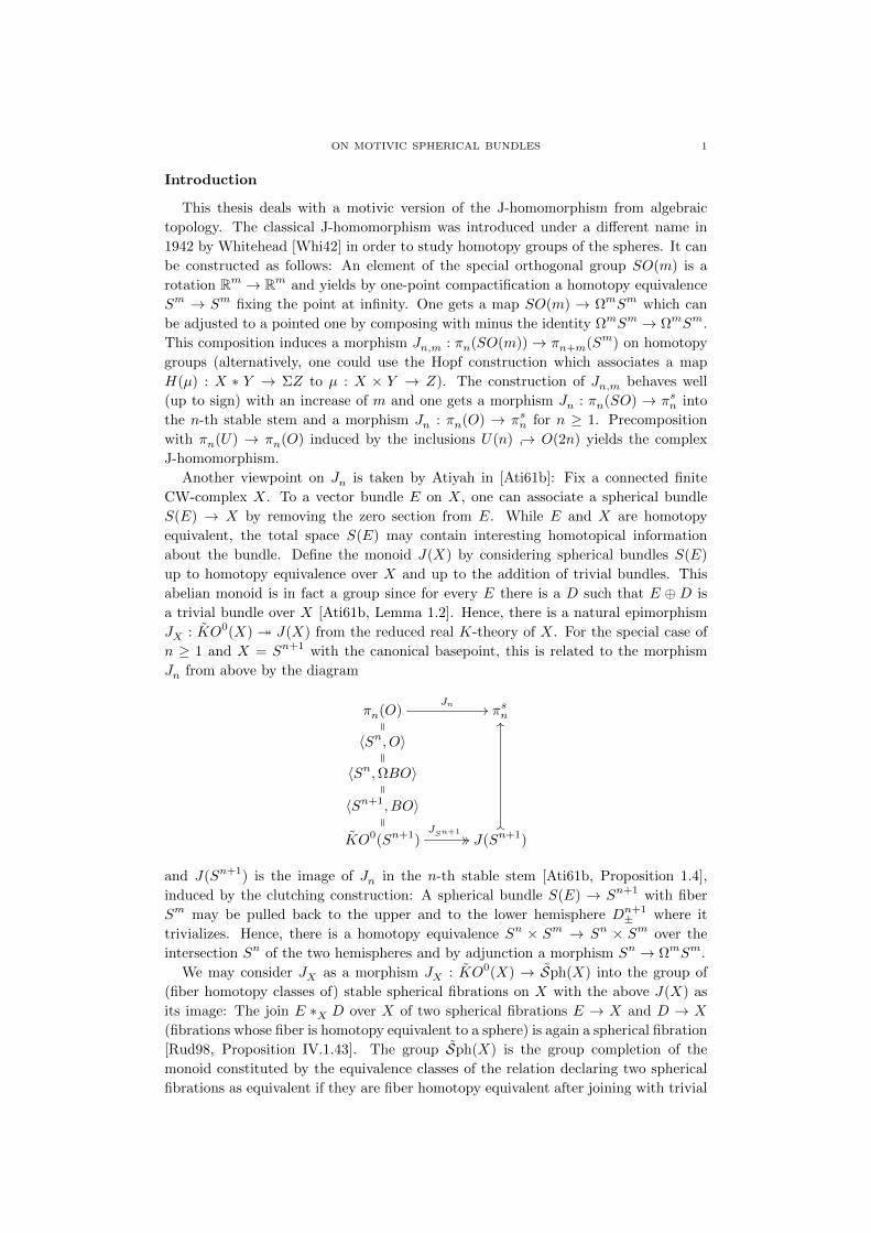
JX : KO0(X) J(X) from the reduced real K-theory of X. For the special case of
n ≥ 1 and X = Sn+1 with the canonical basepoint, this is related to the morphism
Jn from above by the diagram
πn(O)Jn // πsn
〈Sn, O〉
〈Sn,ΩBO〉
〈Sn+1, BO〉
KO0(Sn+1)JSn+1
// // J(Sn+1)OO
OO
and J(Sn+1) is the image of Jn in the n-th stable stem [Ati61b, Proposition 1.4],
induced by the clutching construction: A spherical bundle S(E) → Sn+1 with fiber
Sm may be pulled back to the upper and to the lower hemisphere Dn+1± where it
trivializes. Hence, there is a homotopy equivalence Sn × Sm → Sn × Sm over the
intersection Sn of the two hemispheres and by adjunction a morphism Sn → ΩmSm.
We may consider JX as a morphism JX : KO0(X) → Sph(X) into the group of
(fiber homotopy classes of) stable spherical fibrations on X with the above J(X) as
its image: The join E ∗X D over X of two spherical fibrations E → X and D → X
(fibrations whose fiber is homotopy equivalent to a sphere) is again a spherical fibration
[Rud98, Proposition IV.1.43]. The group Sph(X) is the group completion of the
monoid constituted by the equivalence classes of the relation declaring two spherical
fibrations as equivalent if they are fiber homotopy equivalent after joining with trivial

2 FLORIAN STRUNK
spherical fibrations of arbitrary dimension. The subspace F (m) of ΩmSm consisting
of (basepoint preserving) homotopy equivalences of Sm is a topological monoid under
composition and the classifying space BF of the colimit F has the property that
Sph(X) = [X,BF ] [Sta63].
The Bott periodicity theorem [Bot59] computes all the groups πn(O) and πn(U),
whereas the stable homotopy groups of spheres πsn are hard to describe and not all
known up to now.
n 0 1 2 3 4 5 6 7
πn(O) Z/2 Z/2 0 Z 0 0 0 Z πn(U) 0 Z πsn Z Z/2 Z/2 Z/24 0 0 Z/2 Z/240 . . .
Adams was able to show in a series of papers [Ada63, Ada65a, Ada65b, Ada66]
that, assuming the Adams conjecture, the image of J is always a direct summand,
that J is injective for the Z/2-terms (exept for n = 0) and that for the Z-terms (where
n = 4s−1), the image of J is Z/m(2s) where m(2s) is the denominator of the quotient
Bs/4s of the sth Bernoulli number Bs.
The Adams conjecture states that for each integer k and each vector bundle E over
a finite CW-complex X there exists a natural number t (dependent on k and E) such
that
J(kt(Ψk − 1)E) = 0.
The Adams conjecture was first proven by Quillen [Qui71]. Later, other proofs were
given by Sullivan [Sul74], Friedlander [Fri73] and Becker-Gottlieb [BG75]. An unpub-
lished note of Brown [Bro73] modifies the latter proof avoiding the use of the property
that BF is an infinite loop space. In [Ada63], Adams himself proved the conjecture
for line bundles and two dimensional bundles E → X. The statement of the Adams
conjecture above is linear in E and true for trivial bundles since the Adams operations
Ψk are the identity on them. Hence, a method of proof would be to reduce the ques-
tion successively from bundles with structure group O(m) to bundles with a smaller
structure group until we reach O(1) or O(2) where it holds true by Adam’s result.
The steps in Becker-Gottlieb’s and Brown’s proofs are
O(m) k=dm2 e
O(2k) Σk oO(2) = O(2)k o Σk O(2)
where we will ignore the first easy step. A principal O(2k)-bundle E → X ∼= E/O(2k)
associated to a vector bundle E → X of rank 2k induces morphisms
E/(O(2)× (Σk−1 oO(2)))g−→ E/(Σk oO(2))
f−→ E/O(2k)
where f is a smooth fiber bundle whose fiber O(2k)/(Σk oO(2)) is connected and has
invertible Euler characteristic and where g is an k-sheeted covering space since the
group O(2)× (Σk−1 oO(2)) has index k in Σk oO(2) [Ebe]. Now one argues ‘from both
sides’: If J(f∗E) = 0 then J(E) = 0 and if J(K) = 0 then J(g!K) = 0 where g! is
the geometric transfer [Ati61a]. Finally, one shows that there is a bundle K whose
structure group may be reduced to O(2) such that g!K∼= f∗E. The crucial step in
the proof which uses that BF is an infinite loop space or Brown’s trick is the first step
involving f .
Motivic homotopy theory (also called A1-homotopy theory) is a homotopy theory
of algebraic schemes. Although it is constructed by rather general categorical argu-
ments [MV99], remarkable results like the Milnor conjecture were proven within this
ON MOTIVIC SPHERICAL BUNDLES 3
setting [Voe97]. Many objects and methods from algebraic topology have their motivic
analogues like for instance algebraic K-theory takes the place of topological K-theory.
Nevertheless, many new and interesting difficulties and phenomena arise. For exam-
ple, there are two different types of objects which should be considered as spheres:
A simplicial and an algebraic one, which yield the projective line P1 when they are
smashed together. The behaviour of the algebraic sphere with respect to standard
homotopical constructions seems to be a reason why there is not yet a Recognition
theorem for P1-loop spaces like the one of Boardman-Vogt [BV68, Theorem A,B] in
algebraic topology.
The organization of this text is as follows. In the first section we recall the con-
struction of the motivic homotopy category and provide with Proposition 1.1.22 a
slightly modified version of Morel-Voevodsky’s fibrant replacement functor for one of
its models. Moreover, some properties of homotopy sheaves are discussed. Section 1.3
contains a motivic version of (the second) Mather’s cube theorem and some conse-
quences for motivic fiber sequences inducing exact sequences of A1-homotopy sheaves
are outlined. In the second section, we focus on the stable motivic homotopy cate-
gory. A consequence of Morel’s Motivic Hurewicz theorem which is of importance for
our main result is established in Proposition 2.2.5. Afterwards, we make some ob-
servations on the motivic connectivity of morphisms and use Morel’s results to prove
a Blakers-Massey theorem 2.3.8. The third section begins with recalling the terms
of principal bundles and fiber bundles and describes the procedure of extension and
reduction of their structure group. Next, we outline how results of Morel, Moser, Rezk
and Wendt are used to get motivic fiber sequences from certain bundles. In section
3.3, a motivic J-homomorphism J : K0(X)→ Sph(X) is constructed. Section 4 deals
with vanishing results for the motivic J-homomorphism. We first establish a relation
between the vanishing of the J-homomorphism and Thom classes. A general method
to obtain a transfer morphism due to Ayoub, Hu, May, Rondigs-Østvær and others is
discussed in section 4.2. Then we are ready to prove our main result 4.3.5 which is a
motivic version of the above-mentioned trick of Brown:
Theorem. Let S be the spectrum of a perfect field, F → Yf−→ X a smooth Nisnevich
fiber bundle with an A1-connected base X and an A1-connected fiber F with a dual-
izable suspension spectrum and invertible Euler characteristic χ(F ). Let E → X be
a vector bundle over X. Then J(f∗E) = 0 implies J(E) = 0.
Section 4.4 begins with a Corollary 4.4.2 of a result of Ayoub and Rondigs showing
that for a line bundle E over a projective curve X over a perfect field, J(E ⊗ E) is
zero. Afterwards, we discuss how a reduction process for the vanishing of the J-homo-
morphism could be realized using the established results. We examine a candidate
for a fiber bundle F → Y → X with fiber GLn/NT where NT is the subgroup of
the general linear group consisting of the monomial matrices. In particular for a base
field of characteristic zero, the suspension spectrum of the smooth scheme GLn/NT
is dualizable.
1. Unstable motivic homotopy theory
Remark 1.0.1. Unless no other indication is made, definitions from algebraic geom-
etry are taken from [Liu02]. A base scheme is a noetherian scheme of finite Krull
dimension. Throughout this text, let S denote a base scheme, k a field and SmS the
4 FLORIAN STRUNK
category of smooth schemes of finite type over S. The category SmSpec(k) is abbre-
viated by Smk. An object X → S of SmS is often written as X. Every S ∈ Smk
may serve as a base scheme. Due to the finiteness condition, SmS is an essentially
small category. Smoothness for an object X of SmS may be characterized by the
property, that Zariski-locally on X, the structure morphism X → S factorizes as an
etale morphism U → AnS followed by the projection [Liu02, Corollary 6.2.11].
Basic notations on category theory are taken from [Bor94a] and [Bor94b].
We use [MM92, Section III.2] as a reference for Grothendieck topologies. When
no confusion is possible, we speak of a basis Cov of a Grothendieck topology as of a
Grothendieck topology τ and mean the topology generated by the basis. This is an
abuse of notation since different bases may generate the same Grothendieck topology.
Whenever we speak of a covering of an object in a Grothendieck topology, we mean a
covering for this object in an arbitrary basis for this topology.
The category of Set-valued presheaves on SmS is denoted by Pre or by Pre(S),
if the role of the base scheme has to be emphasized. The symbol Shv or Shv(S)
stands for the category of Set-valued sheaves on SmS with respect to a Grothendieck
topology. The category sPre or sPre(S) of simplicial presheaves or (motivic) spaces
is the category of simplicial objects in Pre. Simplicial sheaves form the category sShv
or sShv(S).
Remark 1.0.2. Although the most-widespread way to define a scheme is to give a
pair (X,OX) consisting of a particular topological space X and a particular sheaf
of rings OX on the open sets of X, it may be intuitively more convenient to think
of a scheme over Spec(k) in the motivic setting as of a particular functor from the
category of finitely generated k-algebras to Set. This equivalent interpretation is
called the functor of points approach. It is explained extensively in [DG70] or in the
first chapter of [Jan87].
Consider the Yoneda embedding
y : k -Algop → Fun(k -Alg,Set)
A 7→ homk -Alg(A,−)
and call a representable yA an affine scheme functor. One wants to formulate the
idea of a scheme functor as being glued out of affine scheme functors in a reasonable
way. To do so, we have to choose along which morphisms affine schemes should be
glued together. An open immersion into an affine scheme functor is a monomorphism
D(I) yA where D(I)(B) = f : A → B |∑x∈I Bf(x) = B for an ideal I of A.
This notion is justified by identifying D(I) evaluated at a field extension K of k with⋃x∈If : A→ K | f(x) 6= 0
which is the complement in yA(K) of the evaluation at K of the closed immersion
V (I) yA where V (I)(B) = f : A → B | ∀x ∈ I : f(x) = 0. In particular for
x ∈ A ∈ k -Alg, the the canonical map A→ Ax defines an open immersion yAx yA
since D((x))(B) = f : A→ B | f(x) ∈ B× = yAx(B).
A set Ui → X of morphisms is a covering if yX(K) is the union of the yUi(K) for
all field extensions K of k. In particular for finitely many open immersions yAxi → yA,
this means that∑Axi = A. These open coverings define a subcanonical topology on
k -Algop called the Zariski topology.

ON MOTIVIC SPHERICAL BUNDLES 5
In order to define the notion of a scheme functor, one defines a compatible notion
of an open immersion into an arbitrary element X of Fun(k -Alg,Set) as a monomor-
phism i : U X such that for any f : yA → X there exists an ideal I of A with
f−1i(U) = D(I). A scheme functor over Spec(k) may now be defined as a sheaf in
the Zariski topology which admits an open covering by affine schemes. To a scheme
(X,OX) one associates a scheme functor B 7→ homSch/k(Spec(B), X). Conversely, for
a scheme functor F the scheme (X,OX) is a left Kan extension. In particular, the
structure sheaf OX may be described as OX(U) = lim OSpec A(j−1(U)) = lim lim Afiwhere j : SpecA → X is the canonical map into the colimit and D((fi)) an open
covering of j−1(U). This provides an equivalence of the two concepts [DG70, I.4.4].
Unfortunately, the definition of a scheme is too restrictive for homotopy theory and
invariant theory since the category of schemes does for example not allow to build
arbitrary quotients. Hence, one weakens the second of the above conditions on a
functor to be a scheme. This leads to the notion of algebraic stacks and, if one gets
rid of the second condition completely, to the whole category of Zariski-sheaves.
Although the functor of points approach may be used as a motivation for the
upcoming categorical constructions, we still use [Liu02] as a reference for our notations.
Remark 1.0.3. The following diagram provides an overview on how the different
model structures and their homotopy categories coming up in this text are designated
where the star refers to the pointed model respectively.
(objectwise) projective
on sPre// local projective
on sPre//
A1-local projective
(or motivic)
on sPre
// unstable
on SpT// stable
on SpT
(objectwise) injective
on sPre
OO
//
local injective
on sPre
OO
//
A1-local injective
on sPre
OO
Hob, Hob∗ Hs, Hs∗ H or HA1
, HA1
∗ SH
1.1. The unstable motivic homotopy category
Remark 1.1.1. The full and faithful Yoneda embedding y : SmS → Pre defined by
yX = homSmS(−, X) commutes with products [MM92, Section I.1] and is a canonical
way to embed SmS into a bicomplete category. This construction has the drawback
of preserving almost no colimits which may be seen as follows: The embedding of the
usual construction
A1 \ 0
// A1
A1 // P1
of the projective line is a pushout diagram in Pre if and only if all presheaves X induce
a pullback diagram
X(P1)
// X(A1)
X(A1) // X(A1 \ 0)
of sets. For the special choice of X = Pic(−), one has Pic(A1) ∼= 0 but Pic(P1) ∼= Z(confer [HS09, Section 2]).
6 FLORIAN STRUNK
For a subcanonical Grothendieck topology, the Yoneda embedding factorizes over
Shv and the diagram ∐yUi ×yX yUj
////
∐yUi yX
is a coequalizer in the category of sheaves for every covering Ui → X in Cov(X).
Hence, one may think of yX as being glued from the covering and the restriction of the
image of the Yoneda embedding to Shv as a way of preserving at least some colimits.
Remark 1.1.2. The isomorphism sPre ∼= Fun(SmopS ×∆op,Set) ∼= Fun(Smop
S , sSet)
is used implicitly throughout the whole text. Composing the Yoneda embedding with
the discrete simplicial set functor Set → sSet provides an embedding of categories
SmS → sPre. Recall that both functors, the discrete embedding and the evaluation at
zero preserve colimits and limits respectively. Considering a simplicial set as constant
in the scheme direction yields an embedding sSet → sPre. This embedding as well
as the evaluation at the terminal scheme preserve colimits and limits. By abuse of
notation, objects are identified by their image under these embeddings respectively.
Remark 1.1.3. For an object U of a category C let C/U be the over category C↓U .
The category Pre is cartesian closed with respect to the product and internal hom
hom(X,Y ) = homPre(X × y(−), Y ) ∼= homPre/y(−)(X × y(−), Y × y(−))
which is a sheaf if Y is a sheaf (considered as a presheaf) [MM92, Proposition III.6.1].
The category SmS/U is a essentially small and often different from the category
SmU unless for example U is etale over S [Gro67, Proposition 17.3.4]. Since there is
an equivalence Pre/yU∼= Pre(SmS/U ), this internal hom may be rewritten further as
homSmS(X ×−, Y ) ∼= homSmS/−
(X ×−, Y ×−) = homSmS/−(X|−, Y |−)
for the special case that X and Y are from SmS . The same holds true when Pre is
replaced by Shv and the slice Grothendieck topologies are used.
The categories sPre and sShv are cartesian closed with internal hom
hom(X,Y ) = hom(X × y(−)×∆(-), Y ).
Remark 1.1.4 (confer Theorem A.1.17). There exists the (objectwise) projective mo-
del structure on the category sPre as well as the (objectwise) injective model structure
on sPre and a monoidal Quillen equivalence
sPreproj sPreinj .
Both model structures are monoidal, proper, combinatorial and simplicial. Their
(equivalent) homotopy categories are denoted by Hob or Hob(S) with morphism sets
[−,−]ob. The tensor for the simplicial enrichment is the categorical product with an
(embedded) simplicial set. The cofibrations for the injective structure are exactly the
monomorphism since limits are calculated objectwise [Bor94a, Proposition 2.15.1]. A
set of generating cofibrations Iproj for the projective structure is given by
U × ∂∆n → U ×∆n
for U ∈ SmS and n ≥ 0 and a set of generating acyclic cofibrations Jproj is
U × Λni → U ×∆n
for n ≥ 1 and 0 ≤ i ≤ n. We will refer to an objectwise projective fibrant simplicial
presheaf in the following just as an objectwise fibrant simplicial presheaf.
ON MOTIVIC SPHERICAL BUNDLES 7
Definition 1.1.5. The Zariski topology Zar on SmS consists of the collections
Zar(X) = fi : Ui → X | each fi is an open immersion, ∪ fi(Ui) = X
of Zariski coverings. It is the topology generated by a complete regular cd-structure
constituted by the Zariski distinguished squares
W
q
//j// Y
p
U //i // X
which are pullback squares such that i and p are open immersions and X = p(Y )∪i(U)
[Voe10, Theorem 2.2]. This defines the (big) Zariski site (SmS ,Zar).
The Nisnevich topology N is on SmS consists of the collections
N is(X) = fi : Ui → X | each fi is etale, ∪fi(Ui) = X,
for all x ∈ X exists some u ∈ f−1i (x), such that k(x) ∼= k(u)
of Nisnevich coverings. It is the topology generated by a complete regular cd-structure
constituted by the Nisnevich distinguished squares
W
q
//j// Y
p
U //i // X
which are pullback squares such that i is an open immersion, p is an etale morphism
and p−1((X \ i(U))red)∼=−→ (X \ i(U))red [Voe10, Proposition 2.17.]. This defines the
(big) Nisnevich site (SmS ,N is).
The etale topology Et on SmS consists of the collections
Et(X) = fi : Ui → X | each fi is is etale, ∪ fi(Ui) = X
and the fppf topology Fppf on SmS of
Fppf(X) = fi : Ui → X | each fi is flat and locally of finite presentation,
∪fi(Ui) = X.
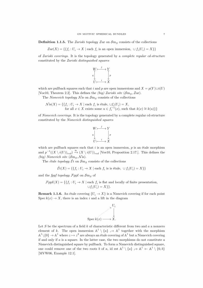
Remark 1.1.6. An etale covering Ui → X is a Nisnevich covering if for each point
Spec k(x)→ X, there is an index i and a lift in the diagram
Ui
Spec k(x) //
::
X.
Let S be the spectrum of a field k of characteristic different from two and a a nonzero
element of k. The open immersion A1 \ a → A1 together with the morphism
A1\0 → A1 where z 7→ z2 are always an etale covering of A1 but a Nisnevich covering
if and only if a is a square. In the latter case, the two morphisms do not constitute a
Nisnevich distinguished square by pullback. To form a Nisnevich distinguished square,
one could remove one of the two roots b of a, id est A1 \ a → A1 ← A1 \ 0, b[MVW06, Example 12.1].

8 FLORIAN STRUNK
Remark 1.1.7. A conservative set of points for the big Zariski site SmS is given by
X 7→ colim(x∈V
open−−−→U)op
X(V ) ∼= colim(x∈Spec(B)→U)op
colimA
(special)
homSmS(Spec(B),Spec(A))
∼= colim colimA
homAlg(A,B)
∼= colimA
homAlg(A, colim B)
∼= colimA
homAlg(A,OU,x)
∼= colimA
homSch/S(Spec(OU,x),Spec(A))
≈ X(Spec(OU,x))
for U (in a skeleton) of SmS and x ∈ U . There is no reason for the scheme Spec(OU,x)
to be of finite type over S. Hence, the notion X(Spec(OU,x)) for an X : SmopS → sSet
is just an intuitive abbreviation for the colimit above.
A conservative set of points for the big Nisnevich site SmS is analogously given by
X 7→ colim(x∈V
nis−−→U)op
X(V ) ∼= colimA
homAlg(A,OhU,x) ≈ X(Spec(OhU,x))
for U (in a skeleton) of SmS and and x ∈ U , where OhU,x is the henselization of the
Zariski stalk OU,x which is again just an abbreviation of the actual colimit (confer
[Gro67, Corollaire 18.6.10] and [Nis87, 1.9]). It is referred to this set of points as to
the canonical set of points.
For a not-necessarily smooth scheme X over S, the functor
homSch/S(−, X) : Smop
S → Set.
is a natural candidate for viewingX as an element of Pre. With the help of the concrete
description of points from above, one can show for example that the non-smooth
coordinate cross Spec k[x, y]/(xy) is isomorphic to the usual pushout A1 ← ∗ → A1
in the category of Zariski-sheaves on SmS . This would not be true when sheaves on
Sch/S were considered instead.
Let K be a field and Spec(K) → S a morphism of SmS . Since OhSpec(K),(0)∼= K,
the functor evaluating an object of Shv(S) at the spectrum of such a field K is a
point of the big Nisnevich site. This can be seen without citing [Nis87, 1.9] as follows:
It suffices to show that evaluating at Spec(K) is a point of the small Nisnevich site
Nis(Spec(K)), this is it commutes with colimits and finite limits. Evaluating at any
U commutes with limits so we have to examine colimits. Every object of this site
is of the form∐ni=1 Spec(Li) → Spec(K), where each field Li is a finite separable
field extension of K and it is a Nisnevich morphism if and only if at least one of
the Li equals K. A presheaf F on this site defines a sheaf if and only if F (∅) ∼= ∗and F (L t L′) ∼= F (L)× F (L′). From this, one observes that evaluating at Spec(K)
commutes with colimits.
Remark 1.1.8. Unless no other indication is made, sheaves are always considered
with respect to the Nisnevich topology in the following. A reason for using the Nis-
nevich topology in motivic homotopy theory is that it shares a good property with
the Zariski and another good one with the etale topology:
• Similar to the Zariski topology, algebraic K-theory has descent properties with
respect to the Nisnevich topology [TT90, Theorem 10.8].
• Similar to the etale topology, an object from Smk of Krull dimension n looks
Nisnevich locally like affine space, this is for a finite separable field extension
ON MOTIVIC SPHERICAL BUNDLES 9
L of k and a point x : Spec (L)→ X there is an isomorphism
X/
(X \ x) ∼= An/
(An \ 0)of Nisnevich sheaves.
Definition 1.1.9. A morphism f : X → Y of simplicial presheaves is called
• local weak equivalence if for all canonical points x (equivalently for all points)
x∗f is a weak equivalence of simplicial sets,
• local projective fibration (respectively local injective fibration) if it has the right
lifting property with respect to projective cofibrations (respectively injective
cofibrations, id est monomorphisms) which are also simplicial weak equiva-
lences.
In the context of a morphism of simplicial sheaves, these properties refer to the un-
derlying morphism of simplicial presheaves.
Theorem 1.1.10 (Blander, Jardine, Joyal). There is a monoidal, proper, combi-
natorial and simplicial model structure on sPre (respectively on sShv) called the
local injective model structure with weak equivalences the local weak equivalences,
cofibrations the monomorphisms and fibrations the local injective fibrations. In
the case of simplicial presheaves, it is the Bousfield localization of the injective
model structure at a certain set consisting of hypercovers (confer [DHI04]).
Moreover, there is a monoidal, proper, combinatorial and simplicial model
structure on sPre (respectively on sShv) called the local projective model structure
with weak equivalences the local weak equivalences, cofibrations the projective
cofibrations and fibrations the local projective fibrations. In the case of simplicial
presheaves, it is the Bousfield localization of the projective model structure at the
morphisms P (Q) → X where P (Q) is a model for the homotopy pushout of the
upper half U ← W → Y of a Nisnevich distinguished square Q (confer [Bla01])
and where we implicitly first choose a skeleton of the category SmS .
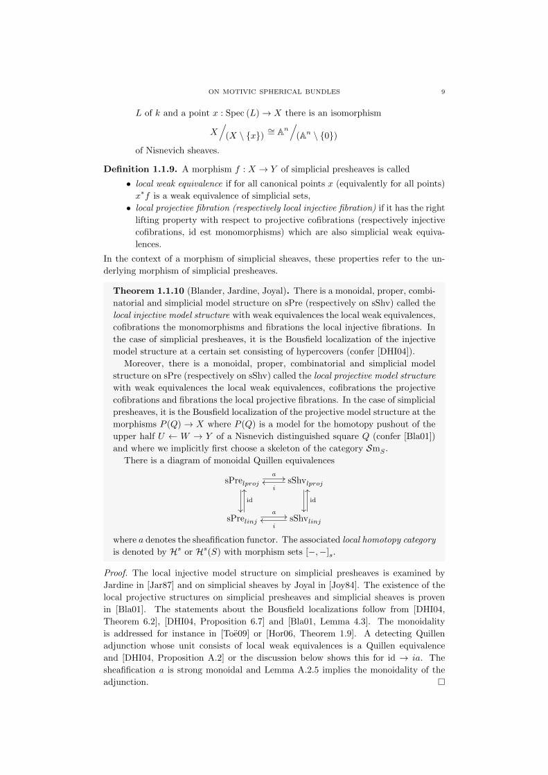
There is a diagram of monoidal Quillen equivalences
sPrelproja //
id
sShvlproji
oo
id
sPrelinja //
OO
sShvlinji
oo
OO
where a denotes the sheafification functor. The associated local homotopy category
is denoted by Hs or Hs(S) with morphism sets [−,−]s.
Proof. The local injective model structure on simplicial presheaves is examined by
Jardine in [Jar87] and on simplicial sheaves by Joyal in [Joy84]. The existence of the
local projective structures on simplicial presheaves and simplicial sheaves is proven
in [Bla01]. The statements about the Bousfield localizations follow from [DHI04,
Theorem 6.2], [DHI04, Proposition 6.7] and [Bla01, Lemma 4.3]. The monoidality
is addressed for instance in [Toe09] or [Hor06, Theorem 1.9]. A detecting Quillen
adjunction whose unit consists of local weak equivalences is a Quillen equivalence
and [DHI04, Proposition A.2] or the discussion below shows this for id → ia. The
sheafification a is strong monoidal and Lemma A.2.5 implies the monoidality of the
adjunction.

10 FLORIAN STRUNK
Remark 1.1.11. Due to [Jar11, Lemma 2.26], injective cofibrations are exactly stalk-
wise cofibrations, id est morphisms which induce cofibrations on all canonical points
(equivalently on all points). The analogue is not true for stalkwise fibrations (or some-
times called local fibrations which conflicts with our notation), which are defined to
be fibrations on all canonical points (equivalently on all points). All local projective
fibrations (and therefore all local injective fibrations) are stalkwise fibrations [Jar11,
Example 6.23].
Remark 1.1.12. The fibrant objects of the local projective model structure on sim-
plicial presheaves may be identified exactly as the flasque simplicial presheaves, which
are defined to be the the objectwise projective fibrant simplicial presheaves F such
that F (∅) ∼= ∗ and for every Nisnevich distinguished square
W
// Y
U // X
the diagram
F (X)
// F (U)
F (Y ) // F (W )
is a homotopy pullback of simplicial sets [Bla01, Lemma 4.1]. In particular, every
Nisnevich distinguished square is a homotopy pushout square (id est a homotopy
colimit diagram in the sense of Remark A.1.21) in the local model structures.
Remark 1.1.13. An important class of local weak equivalences are induced by Cech
complexes. The Cech complex of a morphism f : U → X of presheaves is a simplicial
presheaf C(U) (or C(f)) defined by
Cn(U) = U ×X . . .×X U (n+ 1-times)
with structure maps given by the diagonals and projections together with the canonical
factorization Uif−→ C(U)
pf−→ X of f . The morphism pf is always a stalkwise fibration
but if f is a stalkwise epimorphism, pf is also a local weak equivalence which is
implied by the corresponding statement for simplicial sets on the Nisnevich-points
[MV99, Lemma 2.1.15].
In particular, if Ui → X is a covering and f :∐yUi → yX, this evaluates as
Cn(f) ∼=∐
i0,...,in
yUi0 ×yX . . .×yX yUin .
It is helpful to note that U ×X U ∼= U if U → X is a monomorphism and one writes
shortly
C(f) ∼=(. . .
//////∐i0,i1
Ui0i1////∐i0Ui0
)ob∼ hocolim
(. . .
// ////∐i0,i1
Ui0i1////∐i0Ui0
)for the simplicial presheaf associated to the covering where for the last objectwise weak
equivalence, the Cech complex is viewed as a bisimplicial presheaf since every level can
ON MOTIVIC SPHERICAL BUNDLES 11
be considered as a discrete simplicial presheaf. As the Ui are simplicially discrete, this
object is objectwise weak equivalent to the (simplicially discrete) simplicial presheaf
π0(C(f)) = colim(∐
i0,i1Ui0i1
////∐i0Ui0
)by [Dug98, Lemma 3.3.5]. For a covering, f is a stalkwise epimorphism and there
is a local weak equivalence C(f)∼−→ X as mentioned before. Therefore X may be
considered as a sheaf up to local weak equivalence (confer also [Dug98, Lemma 4.1.6]).
Recall that an objectwiese projective fibrant simplicial presheaf F is said to satisfy
descent with respect to f : U → X if the canonical morphism
F (X)→ holimF (C(f))
is a weak equivalence of simplicial sets and it satisfy descent with respect to a topology
if it satisfies descent for all the coverings of the topology in the above sense. Hence
a simplicially discrete F satisfy descent with respect to a topology if and only if F
is a sheaf for that topology. All local injective fibrant objects F satisfy descent for
the chosen topology defining the local structure [DHI04, Theorem 1.1.]. As mentioned
before, the converse to this statement is not true, even for objectwise injective fibrant
objects [DHI04, Example A.10].
Remark 1.1.14. A fibrant simplicial set viewed as a simplicial presheaf is a fibrant
object in the local model structures. A simplicially constant simplicial presheaf is
fibrant in the local models if and only if it is a sheaf [Jar11, Lemma 5.11]. In particular,
the objects from SmS are fibrant. According to Remark 1.1.1, the presheaf Pic(−)
is not a Nisnevich sheaf and therefore not fibrant in the local models. The objects
from SmS and the simplicial sets are cofibrant for the local model structures as can
be observed by considering the generating cofibratons of Remark 1.1.4.
Since − × ∆1 induces cylinder objects for the local injective model, it follows
from the cofibrancy and fibrancy of the simplicially constant simplicial presheaves
hom(−, U) that there is an embedding SmS → Hs.
Definition 1.1.15. A simplicial presheaf X is called A1-local if the induced map
[Y,X]spr∗−−→ [Y × A1, X]s
is a bijection for all simplicial presheaves Y .
An object X of SmS is called A1-rigid if the induced map
X(U) = homSmS(U,X)
pr∗−−→ homSmS(U × A1, X) = X(U × A1)
is a bijection for all objects U of SmS .
Lemma 1.1.16. Choose either the local injective or the local projective model.
If X is fibrant in this model, then X is A1-local if and only if it is U ×A1 → U-local in the sense of Definition A.3.7. The latter condition writes out as
sSet(U,X)pr∗−−→ sSet(U × A1, X)
being a weak equivalence for all objects U of SmS .
An object of SmS is A1-rigid if and only if it is A1-local.
Proof. We consider the injective situation as the projective is analogous. Choose a
skeleton of the category SmS without changing the notation. Let X be a local injective
fibrant simplicial presheaf. To be U × A1 → U-local is by an enriched version of
12 FLORIAN STRUNK
the Yoneda lemma equivalent to X(U)→ X(U ×A1) being a weak equivalence for all
objects U of SmS . This implies the last statement of the lemma. One has
[U ×A,X]s∼= π0sSet(U ×A,X)∼= [∆0, sSet(U ×A,X)]sSet∼= [∆0,hom(U ×A,X)(S)]sSet∼= [∆0,hom(A,hom(U,X))(S)]sSet∼= [∆0,hom(A, sSet(U,X))(S)]sSet∼= [A, sSet(U,X)]sSet
by the monoidality for all simplicial sets A and objects U of SmS . Hence, the Yoneda
lemma shows that A1-locality implies U × A1 → U-locality of X. The converse
direction is a consequence of lemma A.3.10 since Theorem A.3.8 allows a Bousfield
localization at the set U × A1 → U.
Remark 1.1.17. Choose either the local injective or the local projective model. A
fibrant X in this model is U × A1 → U-local in the sense of Definition A.3.7 if and
only if
sSet(U,X)pr∗−−→ sSet(U × A1, X)
is a weak equivalence for all connected objects U of SmS . Each object U of SmS is
a finite coproduct∐i Ui of connected schemes Ui in the category SmS . Hence, the
statement follows from yU t yV ∼ y(U t V ) being local weakly equivalent, the fact
that sSet(−, X) is a Quillen functor by Definition A.3.1, the equation
sSet(U t V,X) ∼= sSet(U,X)× sSet(V,X)
and the fact that taking π0 commutes with products.
Remark 1.1.18. The projective n-space Pn is not A1-rigid as there are non-constant
morphisms A1 → Pn.
The A1-rigidity of Gm = S ×Spec(Z) Spec(Z)[x, y]/(xy − 1) however may be seen as
follows: As Gm is a Zariski-sheaf, so is homPre(X,Gm) for every presheaf X (confer
Remark 1.1.3). Hence, we may argue Zariski locally and therefore affine. The assertion
follows from the fact, that x 7→ 0 maps the units of A[x] isomorphically to the units
of A.
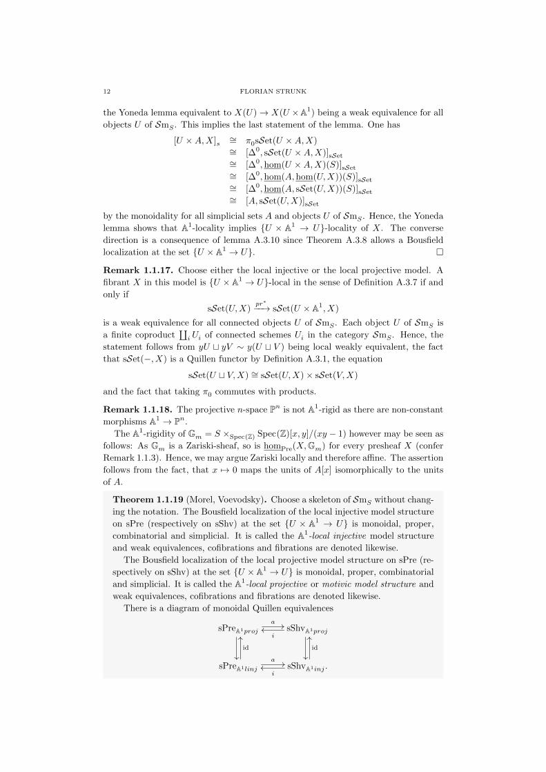
Theorem 1.1.19 (Morel, Voevodsky). Choose a skeleton of SmS without chang-
ing the notation. The Bousfield localization of the local injective model structure
on sPre (respectively on sShv) at the set U × A1 → U is monoidal, proper,
combinatorial and simplicial. It is called the A1-local injective model structure
and weak equivalences, cofibrations and fibrations are denoted likewise.
The Bousfield localization of the local projective model structure on sPre (re-
spectively on sShv) at the set U ×A1 → U is monoidal, proper, combinatorial
and simplicial. It is called the A1-local projective or motivic model structure and
weak equivalences, cofibrations and fibrations are denoted likewise.
There is a diagram of monoidal Quillen equivalences
sPreA1proj
a //
id
sShvA1proji
oo
id
sPreA1linj
a //
OO
sShvA1inj .i
oo
OO

ON MOTIVIC SPHERICAL BUNDLES 13
The associated A1-local homotopy category (or motivic homotopy category) is
denoted by HA1
or HA1
(S) with morphism sets [−,−]A1 or just by H or H(S)
with morphism sets [−,−], if no confusion is possible.
Proof. The existence, the left-properness, combinatoriality and simpliciality of the two
Bousfield localizations follow from Theorem A.3.8 respectively. The right-properness
is a non-trivial issue and was proven for simplicial sheaves in the injective setting
in [MV99, Theorem 2.2.7] and for simplicial presheaves in the injective setting in
[Jar11, Corollary 6.21]. The projective setting is treated in [Bla01, Theorem 3.2]
(The reference to [MV99] in the context of presheaves can be bypassed citing [Jar00a,
Theorem A.5]). The monoidality is a consequence of the monoidality of the local
structure and Remark A.3.9 whose assumptions hold by the existence of a strong
monoidal (with respect to the product) fibrant replacement functor RA1
as discussed
in Remark 1.1.21 below. The horizontal adjunctions of the diagram are monoidal by
Lemma A.2.5 and Quillen adjunctions by [Hir03, Theorem 3.3.20].
Remark 1.1.20. As a consequence of Remark 1.1.14, Remark 1.1.18 and Lemma
A.3.10, the projective n-space Pn is not motivically fibrant, whereas Gm is A1-local
injective fibrant.
The functor −× A1 induces cylinder objects for the A1-local injective model.
Remark 1.1.21. In the discussion around [MV99, Lemma 3.2.6], Morel and Vo-
evodsky construct a fibrant replacement functor RA1
for the A1-local injective model
structure on sShv given by
X 7→ Rs (Rs Sing)|N| Rs
where Rs denotes some local injective fibrant replacement functor and Sing the Suslin-
Voevodsky construction or the singular functor, id est the functor
Sing : sPre → sPre
X 7→ (U, [n]) 7→ X(U ×∆∆n)n
restricted to simplicial sheaves where the cosimplicial object ∆∆(-) : ∆→ SmS is given
by
∆∆n = S ×Spec(Z) Spec(Z)[x0, . . . , xn]/(1−∑xi),
which is non-canonically isomorphic to An as explained after [MV99, Lemma 3.2.5].
According to [MV99, Theorem 2.1.66], one may choose a local injective fibrant re-
placement functor commuting with finite limits. Together with the fact that filtered
colimits of sets commute with finite limits (confer [Bor94a, Theorem 2.13.4]) and to-
gether with the property of the singular functor commuting with all limits, there exists
a strong monoidal A1-local injective fibrant replacement functor.
Proposition 1.1.22. There is an A1-local injective fibrant replacement functor
RA1
on sPre given by
X 7→ Rs (Rsp Sing)|N|
where Rsp denotes some local projective fibrant replacement functor and where Rs
denotes some local injective fibrant replacement functor.
Proof. The method of the proof follows [MV99, Lemma 3.21]. It is to show that
RA1
(X) is A1-local injective fibrant for a simplicial presheaf X. As RA1
(X) is local
injective fibrant, it suffices by Lemma 1.1.16 to show, that RA1
(X) is A1-local but
14 FLORIAN STRUNK
since A1-locality is invariant under local weak equivalence, we may as well prove
that R′(X) = (Rsp Sing)|N|(X) is A1-local. The simplicial presheaf R′(X) is local
projective fibrant as there is a set J ′ of generating acyclic cofibrations detecting the
fibrant objects (confer Remark A.3.8) such that the domains and codomains of these
cofibrations are finitely presentable (confer [DRØ03b, Lemma 2.15.]). Therefore, we
have to show that
R′(X)(U) ∼= sSet(U,R′(X))pr∗−−→ sSet(U × A1, R′(X)) ∼= R′(X)(U × A1)
is a weak equivalence of simplicial sets for every U of SmS by Lemma 1.1.16. Pick
an U of SmS . Since the morphism pr∗ is a section, it suffices to show that for all
basepoints x : ∆0 → R′(X)(U) the map
πi(R′(X)(U), x)
(pr∗)∗−−−−→ πi(R′(X)(U × A1), pr∗(x))
is a surjection for all i ≥ 0. Let x be such a basepoint, i ≥ 0 an integer and
[lb] ∈ πi(R′(X)(U × A1), pr∗(x))
an arbitrary element. As R′(X)(U × A1) is a fibrant simplicial set, the equivalence
class [lb] is represented by a morphism lb : ∂∆i+1 → R′(X)(U × A1) under ∆0 or
equivalently by considering the adjoint maps of simplicial presheaves, it is represented
by a morphism lb : U × A1 × ∂∆i+1 → R′(X). This morphism is under U × A1
or more precisely, the composition U × A1 × ∆0 id×∗−−−→ U × A1 × ∂∆i+1 lb−→ R′(X)
equals U × A1 × ∆0 pr−→ Ux−→ R′(X). Since lb has a finitely presentable domain, it
factorizes through some object nR′(X) = (Rsp Sing)n(X) and by possibly enlarging
n, we assume that the basepoint factorizes as well. Therefore, we obtain a morphism
b : U × A1 × ∂∆i+1 →nR′(X).
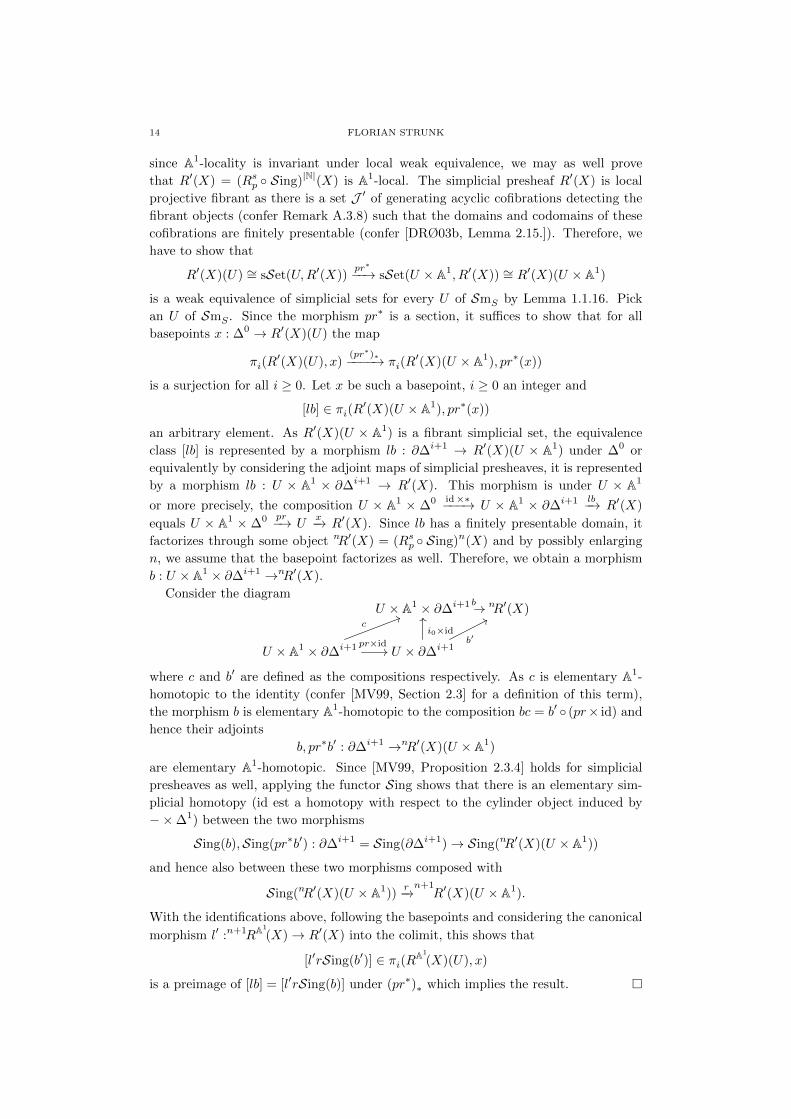
Consider the diagramU × A1 × ∂∆i+1 b // nR′(X)
U × A1 × ∂∆i+1
c55
pr×id// U × ∂∆i+1
i0×id
OO
b′
77
where c and b′ are defined as the compositions respectively. As c is elementary A1-
homotopic to the identity (confer [MV99, Section 2.3] for a definition of this term),
the morphism b is elementary A1-homotopic to the composition bc = b′ (pr× id) and
hence their adjoints
b, pr∗b′ : ∂∆i+1 →nR′(X)(U × A1)
are elementary A1-homotopic. Since [MV99, Proposition 2.3.4] holds for simplicial
presheaves as well, applying the functor Sing shows that there is an elementary sim-
plicial homotopy (id est a homotopy with respect to the cylinder object induced by
−×∆1) between the two morphisms
Sing(b),Sing(pr∗b′) : ∂∆i+1 = Sing(∂∆i+1)→ Sing(nR′(X)(U × A1))
and hence also between these two morphisms composed with
Sing(nR′(X)(U × A1))r−→n+1
R′(X)(U × A1).
With the identifications above, following the basepoints and considering the canonical
morphism l′ :n+1RA1
(X)→ R′(X) into the colimit, this shows that
[l′rSing(b′)] ∈ πi(RA1
(X)(U), x)
is a preimage of [lb] = [l′rSing(b)] under (pr∗)∗ which implies the result.

ON MOTIVIC SPHERICAL BUNDLES 15
Remark 1.1.23. As far as the author knows, it is not known whether Sing(X)
is A1-local for every object X from SmS although there are counterexamples for a
simplicially discrete X [MV99, Example 3.2.7]. According to [Mor12, Theorem 7.2],
Sing(GLn) with n 6= 2 is A1-local for example.
Remark 1.1.24. Following Remark A.4.2, we may equip the categories sPre and sShv
with an initial object S and denote them by sPre∗ or sPre(S)∗ and Shv∗ or sShv(S)∗respectively. One gets pointed, monoidal combinatorial and simplicial analogues of
all the considered model structures by Lemma A.4.5 and Lemma A.4.7 which we
call likewise as in the unpointed setting when no confusion is possible. The models
are right proper since the functor which forgets the basepoint preserves limits and
pushouts (confer Lemma A.4.3).
According to [Hir03, Theorem 3.3.20], one gets the pointed model structures also by
performing a Bousfield localization at those sets obtained by applying the functor (−)∗to the unpointed sets localized at. More precisely and similar for the injective situation,
there is an objectwise projective monoidal, proper, combinatorial and simplicial model
structure on sPre∗∼= Fun(SmS , sSet∗) which can again be localized twice where we
implicitly choose a skeleton of the category SmS : For the first step and to obtain
the local projective model structure, one localizes the objectwise projective model at
the pointed versions P (Q)∗ → X∗ of the morphisms considered in Theorem 1.1.10.
One should note, that applying a canonical point to a morphism of pointed simplicial
presheaves yields a map of pointed simplicial sets. A second Bousfield localization at
the set U∗∧A1∗ → U∗ provides the motivic model structure on sPre∗ with homotopy
category denoted by H∗ or HA1
∗ . For a canonical point p∗, it holds
p∗(X ∧ Y ) = p∗X ∧ p∗Y.
The statement [DRØ03b, Corollary 2.16] shows that the motivic model structure on
sPre∗ is weakly finitely generated and thus shares the properties of Lemma A.1.16
where a set J ′ of generating acyclic cofibrations with the necessary properties may be
constructed by choosing a skeleton of SmS and considering Remark A.3.9.
Moreover, it is shown in [DRØ03b, Lemma 2.20], that smashing with an arbitrary
simplicial presheaves preserves motivic weak equivalences.
1.2. Homotopy sheaves and fiber sequences
Definition 1.2.1. Let X be an element of sPre. One defines the Nisnevich sheaf of
local connected components of X on SmS as
πs0(X) = a[−, X]ob∼= a[−, X]s
and the Nisnevich sheaf of A1-connected components of X on SmS as
πA1
0 (X) = a[−, X]A1 .
The simplicial presheaf X is called locally connected if πs0(X) ∼= ∗ and X is called
A1-connected if πA1
0 (X) ∼= ∗.

16 FLORIAN STRUNK
Remark 1.2.2. The identification of the sheafified objectwise and the sheafified local
homotopy classes follows from the natural isomorphism
π0(p∗X) ∼= π0(colimV
X(V ))
∼= colim π0(X(V ))∼= p∗π0(X(−))∼= p∗aπ0(X(−))∼= p∗a[−, X]ob
for an objectwise fibrant X and a canonical point p applied to the local weak equiva-
lence X → RsX. Moreover, if Rob denotes the objectwise fibrant replacement functor
obtained by applying Kan’s Ex-functor R objectwise, one has
π0(p∗RobX) ∼= π0(Rp∗X) ∼= π0(p∗X).
as R commutes with filtered colimits.
Remark 1.2.3. The Unstable A1-connectivity theorem 1.2.20 implies that a locally
connected simplicial presheaf is also A1-connected. The projective line P1 is an ex-
ample of a non-locally but A1-connected object (confer the diagram of Remark 1.1.1).
The object Gm of SmS is not A1-connected. According to [AM11, Lemma 2.2.11,
Corollary 2.4.4], a connected proper object of Smk is A1-connected if it has a finite
Zariski covering by some Ank such that each intersection of those has a k-point (the last
condition is obsolete if k has infinite many elements). Hence, each projective space
Pn is A1-connected.
If k is a field of characteristic zero, then A1-connectedness of connected proper
objects of Smk is invariant under k-birational equivalence [AM11, Corollary 2.4.6]
where connected objects X and Y from Smk are called k-birationally equivariant, if
there is a k-algebra isomorphism k(X) ∼= k(Y ) of their function fields.
Definition 1.2.4. Let X be an element of sPre∗. For n ≥ 0 one defines the n-th local
homotopy sheaf of X as
πsn(X) = a〈(−)∗ ∧ Sn, X〉ob ∼= a〈(−)∗ ∧ S
n, X〉sand the n-th A1-homotopy sheaf as
πA1
n (X) = a〈(−)∗ ∧ Sn, X〉A1 .
A pointed simplicial presheaf X is called locally n-connected if πsi (X) ∼= ∗ for all i ≤ nand A1-n-connected if πA1
i (X) ∼= ∗ for all i ≤ n. If the morphism X → S is a motivic
weak equivalence, X is called A1-contractible.
Remark 1.2.5. For n = 0 and a pointed simplicial presheaf, this definition is con-
sistent with Definition 1.2.1. It is not true that a morphism of pointed simplicial
presheaves is a local (respectively motivic) weak equivalence, if it induces an isomor-
phism on all local (respectively A1-) homotopy sheaves, even if one takes all basepoints
S → X into account. Instead, one has to consider all morphisms U → X for schemes
U in SmS which may be interpreted as basepoints of SmU . Due to the facts that
homotopy groups of simplicial sets commute with filtered colimits, the canonical Nis-
nevich points are given as filtered colimits and points commute with colimits and
finite limits, one may define local (respectively motivic) weak equivalences as those
morphisms inducing an isomorphism on all local (respectively A1-) homotopy sheaves
with respect to all U → X (confer Remark 1.2.2, [Jar96, Lemma 26]).
ON MOTIVIC SPHERICAL BUNDLES 17
Remark 1.2.6. The A1-homotopy sheaves πA1
n (X) : SmopS → Set interpreted as
simplicially discrete objects of sPre are fibrant in the local structures and one is
tempted to ask, whether they are fibrant in the A1-local structures. This is precisely
to ask, if they are A1-local by Lemma 1.1.16. Although the A1-homotopy presheaves
are A1-local by definition, this is not at all clear for their sheafification. For n ≥ 1 this
was shown by Morel [Mor12] but the case n = 0 remains open [Mor12, Conjecture 12].
Remark 1.2.7. Along with the terms introduced in Section A.6, we may consider
local cofiber sequences and local fiber sequences as well as motivic cofiber sequences
and motivic fiber sequences
F → E → X.
Due to Lemma A.6.7, its dual and Remark A.1.19, we do not have to refer to the
specific injective or projective model when dealing with cofiber sequences and fiber
sequences. Moreover, we do not have to specify the action by Lemma A.6.7. One
should recall the following facts with the help of Lemma A.3.10 and Lemma A.6.7.
• Every diagram A′ → B′ → C ′ isomorphic in Hs∗ to a local cofiber sequence
A → B → C is a local cofiber sequence of the same isomorphism class. The
same holds for motivic cofiber sequences and HA1
∗ instead of Hs∗.• If A→ B → C is a local cofiber sequence, then it is a motivic cofiber sequence.
• Every diagram F ′ → E′ → X ′ isomorphic in Hs∗ to a local fiber sequence
F → E → X is a local fiber sequence of the same isomorphism class. The
same holds for motivic fiber sequences and HA1
∗ instead of Hs∗.• A local fiber sequence F → E → X is a motivic fiber sequence if and only if
RA1
F → RA1
E → RA1
X is a local fiber sequence.
• A local fiber sequence F → E → X is a motivic fiber sequence if and only if
RA1
hofibs(E → X) is isomorphic in the pointed local homotopy category Hs∗to hofibs(RA1
E → RA1
X) ∼ hofibA1
(E → X).
In the sequel, we will consider fiber sequences up to isomorphism without explicitly
mentioning it.
According to Lemma A.6.3 and the exactness of the sheafification functor a, one
gets a long exact sequence of (pointed) local homotopy sheaves
. . .→ πs2(X)→ πs1(F )→ πs1(E)→ πs1(X)→ πs0(F )→ πs0(E)→ πs0(X)
for a local fiber sequence F → E → X and a long exact sequence of (pointed) A1-
homotopy sheaves
. . .→ πA1
2 (X)→ πA1
1 (F )→ πA1
1 (E)→ πA1
1 (X)→ πA1
0 (F )→ πA1
0 (E)→ πA1
0 (X)
for a motivic fiber sequence F → E → X.
Remark 1.2.8. A diagram of simplicial presheaves
P //
C
B // A
is a homotopy pullback in the local homotopical category if and only if it is a homotopy
pullback on all canonical points p∗. This is a consequence of the fact that p∗ sends
local injective fibrations to fibrations of simplicial sets [Jar11, Corollary 4.14] and
commutes with finite limits. As a consequence, a diagram F → E → X of pointed

18 FLORIAN STRUNK
simplicial presheaves is a local fiber sequence if and only if p∗F → p∗E → p∗X is a
fiber sequence of pointed simplicial sets for every canonical point p∗.
By the same argument, a diagram is a homotopy colimit diagram for the local
structures if and only if it is a homotopy colimit diagram on all canonical points.
Definition 1.2.9 (Rezk, [Rez10]). A morphism p : E → X of simplicial presheaves
is called sharp with respect to a model structure, if for each diagram
Ci //
D //
E
p
Zj
∼// Y // X
consisting of pullbacks and a weak equivalence j, the morphism i is a weak equivalence
as well.
Remark 1.2.10. The class of sharp morphisms is closed under pullbacks. All model
structures on simplicial presheaves considered in this text are right proper and hence
every fibration is sharp with respect to the model [Rez98, Proposition 2.2]. Moreover
and with respect to a right proper model, a morphism p is sharp if and only if each
(categorical) pullback diagram
F //
E
p
Y // X
is a homotopy pullback diagram [Rez98, Proposition 2.7]. Since the definition of sharp
morphisms refers to the homotopical category only (confer Remark A.1.19), we define
the notion of locally sharp morphisms as the property of being sharp with respect to
one of the local models and A1-sharp morphisms as being sharp with respect to one
of the A1-local models.
Theorem 1.2.11 (Rezk, [Rez98, Theorem 5.1]). Stalkwise fibrations and pro-
jections out of finite products are locally sharp.
Remark 1.2.12. The previous Theorem 1.2.11 implies in particular, that any mor-
phism between objects from SmS is locally sharp since every map between discrete
simplicial sets is a Kan-fibration.
Lemma 1.2.13. Let
F //
E
p
Yf// X
be a local homotopy pullback diagram of simplicial presheaves such that X is
A1-local. Then the diagram is an A1-homotopy pullback diagram. In particular,
a locally sharp map with an A1-local codomain is A1-sharp.
Proof. Before giving a general proof, we want to mention that for the special case of an
A1-local Y , this can be seen by a more direct argument which is in a similar situation
attributed to Denis-Charles Cisinski [Wen07, Section 4.3]: Choose for instance the

ON MOTIVIC SPHERICAL BUNDLES 19
A1-local injective model. One factorizes f as a motivic weak equivalence Y → Y ′
followed by an A1-local injective fibration Y ′ → X and obtains the diagram
Fi //
E ×X Y ′ //
E
p
Y∼ // Y ′ // // X
consisting of pullbacks. The right square is an A1-homotopy pullback which uses right
properness of the A1-local injective structure. Hence, it suffices to show that i is a
motivic weak equivalence. As X and Y are A1-local injective fibrant by Lemma 1.1.16,
Y ′ is A1-local injective fibrant and the weak equivalence between Y and Y ′ is a local
weak equivalence. Since the original diagram is a local homotopy pullback, i is a local
weak equivalence and hence in particular a motivic weak equivalence.
For the general case, factorize p as a local weak equivalence E → E′ followed by a
local injective fibration p′ : E′ → X. As the diagram of the lemma is a local homotopy
pullback, there is a local weak equivalence F → Y ×X E′. Therefore and to keep the
notation simple, we assume that p is a local injective fibration in the first place.
By [Jar00a, Lemma A.2.4], we can factorize f as a motivic weak equivalence Y → Y ′
followed by an A1-local injective fibration Y ′ → X with the special property that
Y → Y ′ is a so called elementary A1-cofibration. The result then follows by [Jar00a,
Lemma A.3].
Corollary 1.2.14. Let E and X be simplicial presheaves. The projection mor-
phism E ×X → X is A1-sharp.
Proof. As sharp morphisms are stable under basechange, it suffices to show that E → ∗is A1-sharp. The projection E → ∗ is locally sharp by Theorem 1.2.11 and hence the
result follows from Lemma 1.2.13 since the terminal object ∗ is A1-local.
Corollary 1.2.15 (Wendt, [Wen07, Proposition 4.4.1]). Let F → E → X be a
local fiber sequence. If X is A1-local, then it is a motivic fiber sequence.
Theorem 1.2.16 (Morel, [Mor12, Theorem 5.52]). Let S be the spectrum of a
perfect field and F → E → X a local fiber sequence. If X is locally 1-connected,
then it is a motivic fiber sequence.
Remark 1.2.17. Let S be the spectrum of a field. For a simplicial presheaf X, there
is a canonical natural morphism
X → RobX → π0RobX → aπ0R
obX ∼= πs0(X)→ aπ0RA1
RobX ∼= πA1
0 (X)
of simplicial presheaves. Since applying S is a point and there is a fibrant replacement
functor Rop preserving the zero simplices and the latter map of the composition above
is an epimorphism by Theorem 1.2.20, a basepoint S → πA1
0 (X) can be lifted to a
basepoint S → X. This implies that the property of having a basepoint S → X is
invariant under motivic weak equivalence. In particular, every A1-connected simplicial
presheaf X admits a basepoint S → X.
If X is an A1-rigid object of SmS , then the morphism X → πA1
0 (X) is an isomor-
phism of sheaves (and hence a local weak equivalence) but in general one may extract
non-trivial A1-connected components from X, id est for a basepoint S → X, there

20 FLORIAN STRUNK
is an A1-connected pointed simplicial presheaf X ′ such that πA1
n (X ′) ∼= πA1
n (X) for all
n ≥ 1. To obtain X ′, consider the pullback square
X ′ //
RA1
X
f
∗ // πA1
0 (X).
This is a local homotopy pullback square, as the two objects on the right-hand side
are local projective fibrant by Remark 1.1.14 and f is a morphism into a simplicially
discrete object, hence an objectwise fibration. Therefore, there is a local fiber sequence
X ′ → RA1
X → πA1
0 (X). As f is an isomorphism on πs0, one gets that X ′ is locally
connected and by Theorem 1.2.20, it is A1-connected as well. Referring to the local
long exact sequence of Remark 1.2.7, we would get an isomorphism of the higher A1-
homotopy sheaves if X ′ is A1-local. The latter is true as X ′ is a retract of the A1-local
object RA1
X.
The simplicial presheaf X ′ does not have to be scheme if X comes from SmS . In
contrast to topological spaces (of a reasonable type), a simplicial presheaf is usually
not the coproduct of its A1-connected components.
Remark 1.2.18. Let A, B, X and Y be simplicial presheaves. We have
[A tB,X]A1∼= π0sSet(A tB,RA1
X)∼= π0(sSet(A,RA1
X)× sSet(A,RA1
X))∼= π0sSet(A,RA1
X)× π0sSet(B,RA1
X)∼= [A,X]A1 × [B,X]A1
and similarly, since there is an A1-local injective strong monoidal fibrant replacement
functor by Remark 1.1.21, it holds
[A,X × Y ]A1∼= [A,X]A1 × [A, Y ]A1 .
For pointed simplicial presheaves, one gets
〈A ∨B,X〉A1∼= 〈A,X〉A1 × 〈B,X〉A1 ,
〈A,X × Y 〉A1∼= 〈A,X〉A1 × 〈A, Y 〉A1 .
Remark 1.2.19. For integers a and b with a ≥ b ≥ 0, one defines the motivic sphere
Sa,b as Sa,b = Sa−b ∧Gbm. Due to the existence of the Zariski distinguished square
A1 \ 0 //
A1
A1 // P1
there is an isomorphism S2,1 ∼= ΣGm ∼= P1 in the pointed motivic homotopy category.
Theorem 1.2.20 (Morel, Unstable A1-connectivity theorem). Let X be a sim-
plicial presheaf. The canonical morphism πs0X → πA1
0 X is an epimorphism of
sheaves. Moreover for n ≥ 1, if S is the spectrum of a perfect field and if X is
locally n-connected, then it is A1-n-connected.
ON MOTIVIC SPHERICAL BUNDLES 21
Proof. The first statement is [MV99, Corollary 2.3.22] for simplicial sheaves and an
argument is as follows: First, one notes that for a simplicial presheaf Y , there is a
diagram
Y0
(SingY )0
π0Yf// π0SingY
inducing an epimorphism π0Y → π0SingY of presheaves and hence an epimorphism
aπ0Y → aπ0SingY of the associated sheafifications. According to Remark 1.1.21, a
specific A1-local injective fibrant replacement functor is available and one calculates
p∗πs0X = π0(p∗X) → π0(p∗RA1
X)∼= colim(π0p
∗X∼=−→ π0p
∗RsXg−→ π0p
∗SingRsX → . . .)∼= p∗πA1
0 X
for all canonical points p∗ since π0 commutes with filtered colimits and X → RsX is a
local weak equivalence. The assertion follows from the surjectivity of the morphisms
g since to be an epimorphism may be tested on points [Jar11, Lemma 2.26].
The second assertion of the theorem is much harder to prove and is stated for
a pointed simplicial sheaf X as [Mor12, Theorem 5.37]. The result for simplicial
presheaves follows from the observation that the sheafification a does neither change
the local nor the A1-homotopy sheaves.
Corollary 1.2.21. Let S be the spectrum of a perfect field and let a > b ≥ 0 be
integers. Then, the motivic sphere Sa,b is A1-(a− b− 1)-connected.
Proof. The Corollary would follow from the Unstable A1-connectivity theorem 1.2.20
if Sa−b ∧ Gbm would be locally (a − b − 1)-connected. The observation that for all
canonical points p∗ one has
p∗(Sa−b ∧Gbm) ∼= p∗Sa−b ∧ p∗Gbm ∼= Sa−b ∧ p∗Gbmreduces the question to the topological problem of showing that the (a− b)-th sus-
pension of a pointed simplicial set is (a − b − 1)-connected. This is for example a
consequence of the Hurewicz theorem in topology [GJ99, Theorem III.3.7].
Lemma 1.2.22. Let f : E → X be a morphism of pointed simplicial presheaves
with an A1-connected target X. Then, the following conditions are equivalent:
(1) f is a motivic weak equivalence,
(2) πA1
0 (E) ∼= ∗ and πA1
n (f) : πA1
n (E)→ πA1
n (X) are isomorphisms for all n ≥ 1,
(3) the A1-homotopy fiber of f is A1-contractible.
Proof. The implications (1) ⇒ (2) and (1) ⇒ (3) are obvious.
For implication (2) ⇒ (1), let p∗ be an arbitrary canonical point. It is to show
that p∗RA1
f : p∗RA1
E → p∗RA1
X is a weak equivalence of simplicial sets, id est
πn(p∗RA1
E, x) ∼= πn(p∗RA1
X, p∗RA1
f(x)) for all basepoints x : ∆0 → p∗RA1
E. Since
π0(p∗RA1
E) is trivial by assumption, this may be tested at just one arbitrary basepoint
and we choose ∆0 ∼= p∗S → p∗RA1
E induced by the basepoint of E in sPre(S)∗. The
isomorphism of the homotopy groups of simplicial sets is now exactly what is implied
by condition (2) on the point p∗.

22 FLORIAN STRUNK
To prove (3) ⇒ (2), we may choose another model for hofibA1
∼ ∗ as the point-
set fiber of a fibration f ′ : E′ → X ′ of motivically fibrant objects. Let p∗ be a
canonical point. By Remark 1.2.8, p∗f ′ : p∗E′ → p∗X ′ is a fibration of simplicial
sets with contractible fiber p∗hofibA1
. Hence, from the triviality of π0(p∗X ′) it follows
the triviality of π0(p∗E′) and E is A1-connected. Since all homotopy fibers of p∗f ′ at
different basepoints of p∗X ′ are equivalent by [Hir03, Proposition 13.4.7], condition
(2) is implied by the exactness of the sequence of A1-homotopy sheaves.
Lemma 1.2.23. Let X be a pointed simplicial presheaf. Then X is A1-connected
if and only if it path connected in the sense of [CS06, Definition 5.1], this is for
any morphism f : E → X of pointed simplicial presheaves it holds, that f is
a motivic weak equivalence if and only if its A1-homotopy fiber hofibA1
(f) is
A1-contractible.
Proof. Lemma 1.2.22 implies that an A1-connected simplicial presheaf is path con-
nected. For the converse, let X be a path connected but not A1-connected simplicial
presheaf which we assume to be A1-local injective fibrant. Now the same construction
as in Remark 1.2.17 yields a morphism X ′ → X with trivial A1-homotoy fiber. Since
X ′ is A1-connected, this cannot be a weak equivalence.
Proposition 1.2.24. Let X be a pointed A1-connected simplicial presheaf. Let
p : E → X be a morphism in sPre∗ with an A1-connected homotopy fiber F . The
associated fiber sequence F → E → X in H∗ is trivial (confer Definition A.6.1),
id est there is an isomorphism f making the diagram
E
f∼=
p
''F
i77
id×0''
X
F ×Xpr
77
commutative, if and only if there exists a morphism g : E → F in H∗ such that
the composition Fi−→ E
g−→ F is an isomorphism.
Proof. If f exists, the composition g : Ef−→ F ×X pr−→ F with i is an isomorphism by
the definition of id×0 and by f being a morphism under F .
For the other direction, define f as the map into the product F ×X in the category
H∗ induced by g : E → F and p : E → X. Considering the cube
∗ // hofibA1
(f)
∗ ww
//
∗
vv
F // E
f
∗
vv //
Xuu
F // F ×X
∗ ww // Xuu
where the two lower horizontal squares are homotopy pullbacks and all vertical triples
are homotopy fiber sequences, one concludes that the upper horizontal square is a
homotopy pullback as well [Doe98, Lemma 1.4]. This means that ∗ → hofibA1
→ ∗ is
a motivic fiber sequence and it follows hofibA1
(f) ∼ ∗ by Lemma 1.2.22 after choosing
ON MOTIVIC SPHERICAL BUNDLES 23
a model for the fiber sequence. By the same Lemma 1.2.22 it is implied that f is
a weak equivalence since F and X are A1-connected simplicial presheaves and so is
F ×X.
Remark 1.2.25. Theorem A.2.7 furnishes the pointed motivic homotopy category
H∗ with a closed symmetric monoidal structure with involved functors − ∧L − and
homR∗ (−,−). Since every object is cofibrant in the pointed A1-local injective model,
we will by abuse of notation often just write − ∧− instead of − ∧L −.
For integers a, b with a ≥ b ≥ 0, we set Σa,b : sPre∗ → sPre∗ as the functor −∧Sa,b
and moreover Ωa,b : sPre∗ → sPre∗ as the functor hom(Sa,b, RA1
(−)). This notion
behaves well with the simplicial suspension and loop functors where b = 0.
Definition 1.2.26. Let X be an element of sPre(S)∗. For a ≥ b ≥ 0 one defines the
a-th A1-homotopy sheaf with weight b of X as
πA1
a,b(X) = a〈(−)∗ ∧ Sa,b, X〉A1
and the a-th local homotopy sheaf with weight b of X analogously.
Theorem 1.2.27 (Morel, Algebraic loop space theorem). Let S be the spectrum
of a perfect field and X a pointed simplicial presheaf. If X is A1-connected, then
Ω1,1X is A1-connected.
Proof. For a pointed simplicial sheaf X, this is [Mor12, Theorem 5.12] and it was
already observed that local weak equivalences like sheafification do not affect simplicial
or A1-homotopy groups.
Corollary 1.2.28. Let S be the spectrum of a perfect field, a ≥ b ≥ 0 integers
and X a pointed simplicial presheaf. If πA1
a−b,0(X) ∼= ∗, then πA1
a,b(X) ∼= ∗.
Proof. One calculates
πA1
a−b,0(X) ∼= a〈(−)∗ ∧ Sa−b,0, X〉A1
∼= 0∼= a〈(−)∗ ∧ S
0,0,Ωa−b,0X〉A1
⇒ a〈(−)∗ ∧ S0,0,Ωb,bΩa−b,0X〉A1
∼= 0∼= a〈(−)∗ ∧ S
a,b, X〉A1
∼= πA1
a,b(X).
Proposition 1.2.29. Let S be the spectrum of a perfect field and X a pointed
simplicial presheaf. If πA1
0 (X)(S) ∼= ∗, then πA1
0 (Ω1,1X)(S) = ∗.
Proof. It is given that πA1
0 (X)(S) = a〈S∗, X〉A1∼= 〈S∗, X〉A1
∼= ∗ and we have to show
that πA1
0 (Ω1,1X)(S) ∼= 〈S∗,Ω1,1X〉A1
∼= 〈Gm, X〉A1 is trivial. Since the dimension of
Gm is one, there is an isomorphism
〈Gm+, X〉 ∼= H1N is(Gm;πA1
1 (X))
by [Mor12, Lemma 5.12] and H1N is(Gm;πA1
1 (X)) is trivial by [Mor12, Lemma 5.14] as
πA1
1 (X) is a strongly A1-invariant sheaf of groups by [Mor12, Theorem 9].
Corollary 1.2.30. Let S be the spectrum of a perfect field, a ≥ b ≥ 0 integers
and X a pointed simplicial presheaf. If πA1
a−b,0(X)(S) ∼= ∗, then πA1
a,b(X)(S) ∼= ∗.

24 FLORIAN STRUNK
1.3. Mather’s cube theorem and some implications
Remark 1.3.1. A topos is a category equivalent to a category Shv(C) of sheaves on
a Grothendieck site C. The associated sheaf functor a : Pre(C) → Shv(C) commutes
with colimits and finite limits [MM92, Theorem III.5.1]. For a morphism f : Y → X
and a diagram D : I → Shv(C) over X, there is an isomorphism
colimi∈I
(Y ×X D(i)) ∼= Y ×X colimi∈I
D(i)
since this property holds in Set, colimits and limits in Pre(C) are computed objectwise
[Bor94a, Proposition 2.15.1] and the sheafification functor has the above-mentioned
properties. This property is sometimes denoted by saying that colimits are stable
under base change. Considering the two pullback diagrams
E(i)
// E //
Y
f
D(i) // colimD // X
one notes, that colimits are stable under base change, if and only if for every diagram
D, every morphism g : E → colimD and pullback diagram
E(i)
ki // E
g
D(i)ji// colimD
the arrows ki (together with all the arrows E(i)→ E(i′)) constitute a colimit diagram,
this is E is a colimit of the diagram E(−) and the ki are the canonical maps.
Definition 1.3.2 ([Rez98], [Rez10]). A model category C has homotopy descent if the
following two conditions are fulfilled.
(P1) For any morphism f : E → D of diagrams D,E : I → C such that every
square
E(i) //
fi
colimE
D(i) // colimD
is a homotopy pullback and D is a homotopy colimit diagram, it follows that E is
a homotopy colimit diagram.
(P2) For any morphism f : E → D of diagrams such that every square
E(i)E(i→j)
//
fi
E(j)
fj
D(i)D(i→j)
// D(j)
is a homotopy pullback and D and E are homotopy colimit diagrams, it follows
that every square as in (P1) is a homotopy pullback.

ON MOTIVIC SPHERICAL BUNDLES 25
Remark 1.3.3. As discussed in Remark A.1.19, the property of having homotopy
descent is rather a property of the homotopical category associated to a model cate-
gory. Therefore, we will use the term homotopy descent as a property of a homotopical
category obtained by a model category as well.
Remark 1.3.4. Property (P2) is not true for ordinary colimits and base change as
noted in [Rez98, Remark 3.8]. In relation to Remark 1.3.1, one may phrase property
(P1) by saying that homotopy colimits are stable under homotopy base change.
Theorem 1.3.5 (Rezk, [Rez98, Theorem 1.4]). The local homotopical category
has homotopy descent.
Remark 1.3.6. Unfortunately, the motivic homotopical category does not have ho-
motopy descent [SØ10, Remark 3.5].
Theorem 1.3.7. The motivic homotopical category H satisfies the first property
(P1) of Definition 1.3.2 of homotopy descent.
Proof. This proof follows the lines of the first part of the the proof [Rez98, Theorem
1.4]. Choose the A1-injective model structure as a model for the motivic homotopical
category. Take a homotopy pullback square as considered in (P1) and factorize the
right vertical map as a weak equivalence followed by a fibration
colimE∼−→ B colimD.
We assume that D is a homotopy colimit diagram. It is to show that E is a homotopy
colimit diagram. Let A : I → C be the diagram defined by pulling back the map
D(i) → colimD along B → colimD and consider the following cube where Q is a
cofibrant replacement functor for the diagram category with the projective structure
(confer Remark A.3.11).
colimQE
∼
E(i)
∼
// colimE
∼
vv
t
QA(i) // colimQA
A(i)
zz
∼
//
colimA ∼= Bvv
s
QD(i) // colimQD
D(i)zz
∼
// colimDvv
∼
It is to show that t is a weak equivalence. The isomorphism colimA ∼= B follows
from the observation in Remark 1.3.1. The maps E(i) → A(i) are weak equivalences
by the homotopy invariance of homotopy pullbacks and the fact that all squares of
the front face are homotopy pullbacks. The morphism colimQD → colimD is a weak
equivalence because D is a homotopy colimit diagram. The map colimQE → colimQA
is a weak equivalence since it is the homotopy colimit of weak equivalences. Therefore,
it suffices to show that s is a weak equivalence which would follow if we could show
that the lower square of the right face is a categorical pullback, id est
colimQA ∼= B ×colimD colimQD.
26 FLORIAN STRUNK
By Remark 1.3.1, this is implied by
QA(i) ∼= B ×colimD QD(i).
being an isomorphism for every i ∈ I and since the lower front face of the above
diagram is already a pullback, it suffices to show that the lower square of the left face
is a categorical pullback.
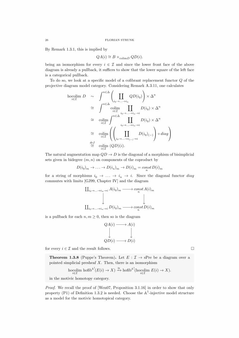
To do so, we look at a specific model of a cofibrant replacement functor Q of the
projective diagram model category. Considering Remark A.3.11, one calculates
hocolimi∈I
D ∼∫ n∈∆
( ∐i0→...→in
QD(i0)
)×∆n
∼=∫ n∈∆
colimi∈I
∐i0→...→in→i
D(i0)×∆n
∼= colimi∈I
∫ n∈∆ ∐i0→...→in→i
D(i0)×∆n
∼= colimi∈I
∐i0→...→i(−)→i
D(i0)(−)
diag
def∼= colimi∈I
(QD)(i).
The natural augmentation map QD → D is the diagonal of a morphism of bisimplicial
sets given in bidegree (m,n) on components of the coproduct by
D(i0)m → . . .→ D(in)m → D(i)m = constn
D(i)m
for a string of morphisms i0 → . . . → in → i. Since the diagonal functor diag
commutes with limits [GJ99, Chapter IV] and the diagram∐i0→...→in→iA(i0)m
// constn
A(i)m
∐i0→...→in→iD(i0)m // const
nD(i)m
is a pullback for each n,m ≥ 0, then so is the diagram
QA(i)
// A(i)
QD(i) // D(i)
for every i ∈ I and the result follows.
Theorem 1.3.8 (Puppe’s Theorem). Let E : I → sPre be a diagram over a
pointed simplicial presheaf X. Then, there is an isomorphism
hocolimi∈I
hofibA1
(E(i)→ X)∼=−→ hofibA1
(hocolimi∈I
E(i)→ X).
in the motivic homotopy category.
Proof. We recall the proof of [Wen07, Proposition 3.1.16] in order to show that only
property (P1) of Definition 1.3.2 is needed. Choose the A1-injective model structure
as a model for the motivic homotopical category.
ON MOTIVIC SPHERICAL BUNDLES 27
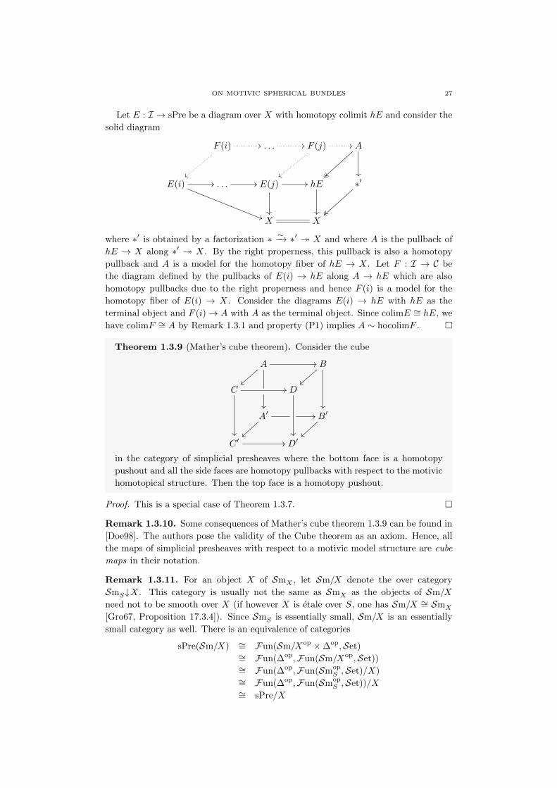
Let E : I → sPre be a diagram over X with homotopy colimit hE and consider the
solid diagram
F (i) //
||
. . . // F (j)
||
// A
~~~~
E(i) //
))
. . . // E(j)
// hE
∗′
X X
where ∗′ is obtained by a factorization ∗ ∼−→ ∗′ X and where A is the pullback of
hE → X along ∗′ X. By the right properness, this pullback is also a homotopy
pullback and A is a model for the homotopy fiber of hE → X. Let F : I → C be
the diagram defined by the pullbacks of E(i) → hE along A → hE which are also
homotopy pullbacks due to the right properness and hence F (i) is a model for the
homotopy fiber of E(i) → X. Consider the diagrams E(i) → hE with hE as the
terminal object and F (i)→ A with A as the terminal object. Since colimE ∼= hE, we
have colimF ∼= A by Remark 1.3.1 and property (P1) implies A ∼ hocolimF .
Theorem 1.3.9 (Mather’s cube theorem). Consider the cube
A //
B
C
//
D
A′
~~
// B′
~~
C ′ // D′
in the category of simplicial presheaves where the bottom face is a homotopy
pushout and all the side faces are homotopy pullbacks with respect to the motivic
homotopical structure. Then the top face is a homotopy pushout.
Proof. This is a special case of Theorem 1.3.7.
Remark 1.3.10. Some consequences of Mather’s cube theorem 1.3.9 can be found in
[Doe98]. The authors pose the validity of the Cube theorem as an axiom. Hence, all
the maps of simplicial presheaves with respect to a motivic model structure are cube
maps in their notation.
Remark 1.3.11. For an object X of SmX , let Sm/X denote the over category
SmS↓X. This category is usually not the same as SmX as the objects of Sm/X
need not to be smooth over X (if however X is etale over S, one has Sm/X ∼= SmX
[Gro67, Proposition 17.3.4]). Since SmS is essentially small, Sm/X is an essentially
small category as well. There is an equivalence of categories
sPre(Sm/X) ∼= Fun(Sm/Xop ×∆op,Set)∼= Fun(∆op,Fun(Sm/Xop,Set))∼= Fun(∆op,Fun(Smop
S ,Set)/X)∼= Fun(∆op,Fun(Smop
S ,Set))/X∼= sPre/X

28 FLORIAN STRUNK
omitting the notion for the Yoneda embedding and the discrete simplicial object func-
tor. Hence, the (objectwise) projective model structure on sPre(Sm/X) can be identi-
fied with the over model structure of Theorem A.3.12 with respect to the (objectwise)
projective model sPre. The equivalence Pre(Sm/X) ∼= Pre(SmS)/X in the third step
is given as follows: An object E → X in Pre(SmS)/X is mapped to the presheaf
sending the object u : U → X of Sm/X to the set E(u) of lifts in the diagram
E
p
Uu //
l
>>
X
again omitting the notion for the Yoneda embedding. Conversely, an object E(−) of
Pre(Sm/X) is mapped to the presheaf sending the object U of SmS to E(U) and
E(U) =∐
u:U→XE(u)→
∐u:U→X
∗ = X(U).
This equivalence can be promoted to an equivalence Shv(Sm/X) ∼= Shv(SmS)/X
of topoi, where Sm/X carries the obvious Grothendieck topology which is gener-
ated by the over basis [MM92, Exercise III.8.(b)]. Hence, since a model structure
is determined by its cofibrations and weak equivalences, the local projective model
structure on sPre(Sm/X) can be identified with the over model structure with re-
spect to the local projective model structure on sPre (confer [Bla01, Theorem 1.6]).
The author considers it as unlikely, that for every X in SmS the model structure on
sPre(Sm/X) obtained by a Bousfield localization of the above mentioned local model
at the U × A1 → U can be identified with the over model structure on sPre/X with
respect to the motivic model structure on sPre.
In what follows, we will use of the over model structure on sPre/X with respect to
the A1-local injective or the motivic model structure on sPre only.
Remark 1.3.12. Please note, that for the following Definition 1.3.13 we refer to the
convetion of Definition A.1.18 of considering hocolim and hocolim as functors to the
category of simplicial presheaves.
Definition 1.3.13. Let X be a simplicial presheaf. For morphisms X → E and
X → D in sPre, one sets E ∨hX D = hocolim(E ← X → D) as the homotopy wedge
of E and D over X. For morphisms E → X and D → X in sPre one defines
E ×hX D = holim(D → X ← E) as the homotopy product of E and D over X.
If X → E → X and X → D → X are the identities respectively, one defines
E ∧hX D = hocofib(E ∨hX Dt−→ E ×hX D)
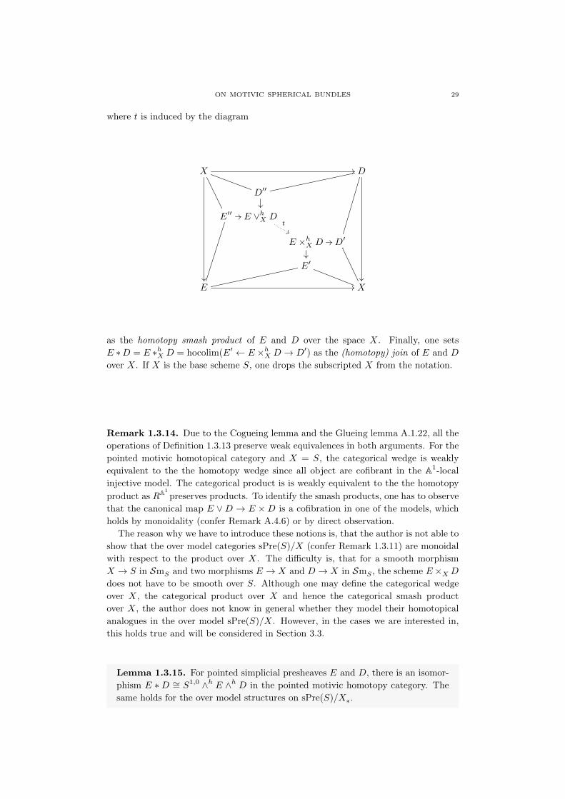
ON MOTIVIC SPHERICAL BUNDLES 29
where t is induced by the diagram
X
// D
D′′
E′′ // E ∨hX Dt&&
E ×hX D //
D′
E′
E // X
as the homotopy smash product of E and D over the space X. Finally, one sets
E ∗D = E ∗hX D = hocolim(E′ ← E ×hX D → D′) as the (homotopy) join of E and D
over X. If X is the base scheme S, one drops the subscripted X from the notation.
Remark 1.3.14. Due to the Cogueing lemma and the Glueing lemma A.1.22, all the
operations of Definition 1.3.13 preserve weak equivalences in both arguments. For the
pointed motivic homotopical category and X = S, the categorical wedge is weakly
equivalent to the the homotopy wedge since all object are cofibrant in the A1-local
injective model. The categorical product is is weakly equivalent to the the homotopy
product as RA1
preserves products. To identify the smash products, one has to observe
that the canonical map E ∨D → E ×D is a cofibration in one of the models, which
holds by monoidality (confer Remark A.4.6) or by direct observation.
The reason why we have to introduce these notions is, that the author is not able to
show that the over model categories sPre(S)/X (confer Remark 1.3.11) are monoidal
with respect to the product over X. The difficulty is, that for a smooth morphism
X → S in SmS and two morphisms E → X and D → X in SmS , the scheme E×X Ddoes not have to be smooth over S. Although one may define the categorical wedge
over X, the categorical product over X and hence the categorical smash product
over X, the author does not know in general whether they model their homotopical
analogues in the over model sPre(S)/X. However, in the cases we are interested in,
this holds true and will be considered in Section 3.3.
Lemma 1.3.15. For pointed simplicial presheaves E and D, there is an isomor-
phism E ∗D ∼= S1,0 ∧h E ∧h D in the pointed motivic homotopy category. The
same holds for the over model structures on sPre(S)/X∗.

30 FLORIAN STRUNK
Proof. For a diagram
E ∨h D //
zz
D
wwE
//
∗
E ×h D //
zz
D
ww
E
//
E∗D
E ∧h D
zz
// ∗ww
∗ // S1,0 ∧h E ∧h D
consisting of cofiber sequences in all but the front right vertical column and homotopy
pushouts in the upper and the middle horizontal square, one gets that the front right
vertical column is a cofiber sequence if and only if the bottom square is a homotopy
pushout [Doe98, Lemma 1.4]. This implies the result as ∗ → E∗D → S1,0∧hE∧hD is
a cofiber sequence if and only if its latter morphism is an isomorphism in the homotopy
category.
Remark 1.3.16. Considering the Zariski (and thus Nisnevich) distinguished square
(An − 0)× (A1 − 0) //
An × (A1 − 0)
(An − 0)× A1 // An+1 − 0
for n ≥ 1, one gets an isomorphism (An−0)∗S1,1 ∼= An+1−0, hence An−0 ∼= S2n−1,n
and therefore S1,0 ∧ (An − 0) ∼= (P1)∧n in the pointed motivic homotopy category.
Lemma 1.3.17. The following statements are true with respect to the pointed
motivic homotopical category, pointed simplicial presheaves X and Y and a mo-
tivic fiber sequence F → E → X.
(1) X ∗ ∗ ∼= ∗ and X ∗ S0 ∼= S1,0 ∧X,
(2) S1,0 ∧ (X × Y ) ∼= (X ∗ Y ) ∨ (S1,0 ∧X) ∨ (S1,0 ∧ ΣY ),
(3) There is a motivic fiber sequence ΣΩX → X ∨X → X,
(4) There is a motivic fiber sequence ΩX ∗ ΩY → X ∨ Y → X × Y ,
(5) There is a motivic fiber sequence F ∗ ΩX → hocofib(F → E)→ X,
(6) There is a motivic fiber sequence ΩX ∗ ΩX → ΣΩX → X
Proof. All these statements are abstract facts about suitable model categories in which
Mather’s cube theorem 1.3.9 holds. Statement (1) is clear. Statement (2) is [Doe98,
Corollary 2.13] and (3) follows directly from Puppe’s theorem 1.3.8 applied to the
diagram ∗ ← X → ∗ over X. The assertion (4) is [Doe98, Proposition 4.6] and
statement (5) is [Doe98, Corollary 4.3]. Proposition (6) follows from (5) applied to
the fiber sequence ΩX → ∗ → X.

ON MOTIVIC SPHERICAL BUNDLES 31
2. Stable motivic homotopy theory
2.1. The stable motivic homotopy category
Remark 2.1.1. We are going to apply the construction of Section A.5 in order to get
a stable version of the pointed motivic homotopy category with respect to the smash
product with S2,1 (which is motivically weak equivalent to P1). From this it follows
the invertibility of the smash with both, the simplicial cycle S1,0 and the algebraic
cycle S1,1 = Gm.
Remark 1.1.24 introduces the motivic (I∗,J∗)-cofibrantly generated, proper, com-
binatorial, simplicial, monoidal and pointed model structure on sPre(S)∗ with a cofi-
brant unit S0. It is well stabilizable by [DRØ03b, Corollary 2.16]. In order to get a
cofibrant object T for the method of Section A.5, one uses the simplicial mapping cylin-
der construction of Lemma A.3.6 with respect to the monomorphism (A1− 0)∗ A1∗
to get a factorization (A1 − 0)∗ Cyl∼−→ A1
∗. The pushout
(A1 − 0)∗// //
Cyl
∗ // // T
yields a cofibrant object T which is as a pushout of finitely presentable objects again
finitely presentable. Since this pushout is a homotopy pushout as well, the homotopy
cofibers of the two horizontal morphisms coincide. Hence, there is an isomorphism
T ∼= P1 in the pointed motivic homotopy category (confer Remark 1.3.16).
The object T is weakly equivalent to a symmetric object in the sense of Definition
A.5.17 by [Jar00a, Lemma 3.13] (confer also [DRØ03b, Lemma 2.24]) and therefore
the conclusions of Theorem A.5.19 hold.
Definition 2.1.2. As observed in the previous Remark 2.1.1, there is by the results
of Section A.5 a proper, combinatorial, simplicial and pointed model structure on
the category SpT (or SpT (S)) of motivic T -spectra (or motivic spectra), the unstable
motivic model structure. Moreover, there is a proper, combinatorial, simplicial and
pointed model structure on the category SpT , the stable motivic model structure and
its homotopy category is denoted by SH.
Remark 2.1.3. Even though the stable motivic homotopy category SH can be
equipped with a symmetric monoidal structure in a reasonable way as done below, the
category of motivic spectra SpT does not serve as a good model for this symmetric
monoidal structure in the sense of Theorem A.2.7 [Lew91].
The category SpΣT (or SpΣ
T (S)) of motivic symmetric T -spectra as constructed in
[Hov01b] may be equipped with a closed symmetric monoidal structure [Hov01b, The-
orem 8.3] such that there is a monoidal adjunction
Σ∞T : sPre∗ SpΣT : (−)0.
Moreover, there is an adjunction
V : SpT SpΣT : U
relating the ordinary and the symmetric motivic T -spectra and factorizing (ΣT , (−)0)
through its non-symmetric analogue. The category SpΣT may be furnished with a left
proper combinatorial, simplicial and monoidal pointed stable motivic model structure
as done in [Hov01b, Theorem 8.11] such that (ΣT , (−)0) becomes a monoidal Quillen

32 FLORIAN STRUNK
adjunction. The stable model structure on motivic symmetric T -spectra is also right
proper which does not follow from the general arguments of [Hov01b] and may be
seen as follows: Replacing injective objects by unstably cofibrant objects, the proof
of [Jar00a, Proposition 4.8] can be adopted to show that U : SpΣT → SpT reflects
stable weak equivalences. Hence, the projective analogue of the properness argument
[Jar00b, Theorem 12] holds. Moreover, the projective version of [Jar00b, Corollary
11] and [Jar00b, Theorem 13] imply that (V,U) is a Quillen equivalence.
Lemma 2.1.4 (Stability lemma). Let X and Y be motivically cofibrant and
finitely presentable pointed simplicial presheaves. Then, there exists an isomor-
phism
u : Σ∞T X∼=−→ Σ∞T Y
in the stable motivic homotopy category SH if and only if there exists a natural
number n and an isomorphism
v : ΣnTX∼=−→ ΣnTY
in the pointed motivic homotopy category H∗.
Proof. For a motivically cofibrant and finitely presentable pointed simplicial presheaf
X and a motivic T -spectrum E, there is an isomorphism
〈Σ∞T X,E〉SH ∼= 〈Σ∞T X,Θ∞T RE〉SH
∼= 〈X, (Θ∞T RE)0〉H∗∼= 〈X, colimnΩnTREn〉H∗∼= π0sSet∗(X, colimnΩnTREn)∼= colimnπ0sSet∗(X,Ω
nTREn)
∼= colimn〈X,ΩnTREn〉H∗∼= colimn〈Σ
nTX,REn〉H∗∼= colimn〈ΣnTX,En〉H∗
where R is a fibrant replacement functor for the unstable model structure (respectively,
denoted by abuse of notation by the same symbol, for the pointed motivic model)
and where the fifth isomorphism exists as the object X ∧ ∆n∗ is finitely presentable
[DRØ03b, Lemma 2.5]. The isomorphism above is natural with respect to morphisms
of pointed simplicial presheaves between motivically cofibrant and finitely presentable
pointed simplicial presheaves X and with respect to morphisms in SH between motivic
T -spectra E.
Let Y be another motivically cofibrant and finitely presentable pointed simplicial
presheaf and consider the special case of E = Σ∞T Y . The morphisms of the filtered
diagram for the colimit on the right-hand side of the isomorphism are given by
〈ΣnTX,RΣnTY 〉H∗LΣ−−→ 〈ΣTΣnTX,ΣRΣnTY 〉H∗
σ∗−→ 〈Σn+1T X,RΣn+1
T Y 〉H∗(confer Definition A.5.15) and hence the isomorphism from the right to the left is on
components of the colimit given as
〈ΣnTX,ΣnTY 〉H∗
LΣ∞T−−−→ 〈Σ∞T ΣnTX,Σ∞T ΣnTY 〉SH
∼= 〈ΣnTΣ∞T X,ΣnTΣ∞T Y 〉SH
L[−n]−−−−→ 〈Σ∞T X,Σ∞T Y 〉SH,
(confer Remark A.5.8 and Theorem A.5.19) which is again natural with respect to
morphisms of pointed simplicial presheaves between motivically cofibrant and finitely
ON MOTIVIC SPHERICAL BUNDLES 33
presentable pointed simplicial presheaves X and Y . The statement follows now from
naturality and the fact that the identity is represented by the identity for some n.
Corollary 2.1.5. Let f : X → Y be a morphism of motivically cofibrant and
finitely presentable pointed simplicial presheaves. Then Σ∞T f is a stable motivic
weak equivalence if and only if there exists a natural number n such that ΣnT f is
a motivic weak equivalence.
Remark 2.1.6. If S is the spectrum of the complex numbers, there is a complex
realization functor
ReC : sPre(Spec C)→ T op
into the category of compactly generated topological spaces given as the left Kan
extension of the functor SmS ×∆→ T op sending (U, [n]) to U(C)×|∆n| where U(C)
is the set of complex points of U with the analytic topology. This functor is symmetric
monoidal with respect to the product. It has a right adjoint given by SingC(X) =
homT op((−)(C) × ∆(-), X) and induces a functor on the pointed categories which is
denoted likewise and is symmetric monoidal with respect to the smash product. By
a similar argument as in the proof of [PPR07, Theorem A.4.1], both functors are left
Quillen functors with respect to the motivic model structure.
There is a (symmetric monoidal) model structure on the category of topological
(symmetric) CP 1-spectra whose homotopy category is equivalent as a symmetric mo-
noidal and triangulated category to the ordinary stable homotopy category of spaces
[PPR07, Theorem A.7.1] and the complex realization functor ReC induces a (strict
symmetric monoidal) left Quillen functor from the model category of (symmetric)
motivic P1-spectra (confer [Hor06, Theorem 1.12]) into the former (symmetric) one
[PPR07, Theorem A.7.2].
Definition 2.1.7. Let X be an element of SpT . For a ≥ b ≥ 0 one defines the a-th
(T -)stable homotopy sheaf with weight b of X as
πsta,b(X) = a〈Σ∞T ((−)∗ ∧ S
a,b), X〉SHand with the usual convention of smashing with the respective negative indices on the
right-hand side, this sheaf can be defined for all integers a and b. A spectrum X is
called (T -)stably contractible if the morphism X → S is a stable weak equivalence.
One writes just πsta,b for the group πst
a,b(S)(S) = 〈Sa,b,S〉SH.
Remark 2.1.8. For a motivic T -spectrum X and integers a ≥ b ≥ 0, one calculates
πsta,b(X) ∼= a〈Σ∞T ((−)∗ ∧ S
a,b), X〉SH∼= a〈(−)∗ ∧ S
a,b, (Θ∞T RX)0〉A1
∼= a〈(−)∗ ∧ Sa,b, colim
mΩmT RXm〉A1
∼= colimm
a〈(−)∗ ∧ Sa,b,ΩmT RXm〉A1
∼= colimm
a〈(−)∗ ∧ Sa+2m,b+m, Xm〉A1
∼= colimm
πA1
a+2m,b+m(Xm)
where R is a fibrant replacement functor for the unstable model structure. The fourth
equality holds as the object U∗ ∧ Sa,b ∧∆n
∗ is finitely presentable for any U in SmS
by [DRØ03b, Lemma 2.5]. In accordance with the usual convention, we may define
the sheaf πsta,b(X) with respect to all integers a and b and it holds
πsta−2l,b−l(X) ∼= πst
a,b(X[l]).

34 FLORIAN STRUNK
A morphism f : X → Y of spectra is a stable weak equivalence if and only if it
induces an isomorphism πsta,b(f) for all integers a and b [Hov99, Theorem 7.3.1].
Remark 2.1.9. Let S be the spectrum of a perfect field k. As far as the author
is informed, there is not much known about the groups πsta,b. The Unstable A1-
connectivity theorem together with Corollary 1.2.30 imply that πsta,b∼= 0 whenever
a < b. For a = b Morel proved in [Mor04, Theorem 6.2.1] and [Mor12, Corollary
5.42 ] the existence of an isomorphism πsta,a∼= KMW
−a (which can be promoted into an
isomorphism of a-graded rings) where it should be recalled that KMW0 is isomorphic
to the Grothendieck-Witt ring GW (k).
2.2. A consequence of the motivic Hurewicz theorem
Remark 2.2.1. Let the base scheme S be the spectrum of a perfect field. Applying
the canonical monoidal adjunction Z : Set Ab : U degree-wise induces a monoidal
adjunction Z : sSet sAb : U where the the right adjoint factorizes through the
subcategory of Kan complexes. This can be promoted into a monoidal Quillen adjunc-
tion furnishing sAb with the model structure where weak equivalences and fibrations
are detected by the right adjoint [GJ99, Theorem III.2.8]. As a simplicial abelian
group is canonically pointed, one has a monoidal Quillen adjunction sSet∗ sAb
with left adjoint Z(∗ → X) = Z(X)/Z(∗). This construction is compatible with the
canonical monoidal Quillen equivalence from simplicial sets to pointed simplicial sets.
The Dold-Kan correspondence is an equivalence of categories
N : sAb Ch≥0 : K
with the property that πn(X, 0) ∼= Hn(NX). The homotopy groups of a simplicial
abelian group do not depend on the basepoint [GJ99, Corollary III.2.3]. Furthermore,
one has an adjunction
i : Ch≥0 Ch : t
where i is the inclusion and t is the good truncation defined by t(X)n = Xn if n ≥ 1
and t(X)0 = ker(X0 → X−1), both preserving isomorphisms on homology.
Applying this to the category Ch(S) ∼= Ch(Fun(SmopS ,Ab)) ∼= Fun(Smop
S , Ch), the
composition of the above-mentioned adjunctions yields an adjunction
Z : sPre(S)∗ Ch(S) : U
denoted in this way by abuse of notation. There are again several viewpoints for model
structures on Ch(S) as for instance [Jar03], developing a model structure on Ch(S) as
a stabilization in the sense of Section A.5.
According to [Fau06, Theorem 6.1], there is a proper, cofibrantly generated, mo-
noidal and pointed model structure on Ch(S) where the weak equivalences are the
morphisms inducing homology isomorphisms on all (canonical) points. In particular,
a morphism of chain complexes is a weak equivalence if and only if it induces an
isomorphism on all homology sheaves aHn(−). The adjunction (Z, U) is a Quillen
adjunction with respect to the local projective model structure on sPre(S)∗ and the
just defined stalkwise model structure on Ch(S) since the left adjoint sends generating
cofibrations to cofibrations and weak equivalences to weak equivalences. The stalkwise
model structure is a Bousfield localization of a projective model structure on Ch(S)
(confer [CH02] and [Hov99, Section 2.3]).

ON MOTIVIC SPHERICAL BUNDLES 35
On the category Ch′(S) = Ch(ShvAb(S)) of chain complexes of sheaves SmopS →
Ab, one has the injective model structure as ShvAb(S) is a Grothendieck category
(id est a cocomplete abelian category in which filtered colimits commute with finite
limits with an object G, called a generator, such that hom(G,−) is faithful) [Hov01a].
Sheafification defines a Quillen equivalence
a : Ch(S) Ch′(S) : i
where Ch(S) is furnished with the stalkwise model structure [Fau06, Proposition 6.2].
In the injective model Ch′(S), every object is cofibrant and the fibrant objects are
sometimes denoted as those complexes of injective sheaves which are K-injective (con-
fer [Spa88]). In particular, any bounded above complex of injective sheaves is fibrant
[Hov01a, Proposition 2.12] and there is a computable fibrant replacement given by the
right Cartan-Eilenberg resolution (confer [Wei94, 5.7.9]).
One advantage of the stalkwise model structure on Ch(S) however is the monoidality
with respect to the canonical tensor product of chain complexes
(Z(X)⊗ Z(Y ))n =⊕i
Z(X)i ⊗ Z(Y )n−i
(confer [Fau06, Lemma 4.4]). The adjunction (Z, U) is not a strong monoidal ad-
junction with respect to this canonical tensor product. Fortunately, the Eilenberg-
Zilber theorem [GJ99, Theorem IV.2.4] implies the existence of a weak equivalence
Z(X) ⊗ Z(Y ) → Z(X ∧ Y ) yielding an isomorphism aHn(X) ∼= aHn+1(ΣX) for a
pointed simplicial presheaf X together with the isomorphism Z(ΣX) ∼= Z(X)[1] where
[1] denotes a shift of the chain complex to the left, id est C[1]n = Cn−1.
For a pointed simplicial presheaf X, one defines the n-th reduced local (Nisnevich)
homology sheaf as
Hsn(X) = aHn(Z(X))
∼= a[Z[Sn ∧ (−)∗], Z[X]]∼= a〈Sn ∧ (−)∗, U Z(X)〉s∼= πsn(U Z(X))
where we do not have to make a fibrant replacement before applying the right adjoint as
it preserves weak equivalences. Setting Hsn(X) = Hs
n(X∗) as the n-th local (Nisnevich)
homology sheaf, one has Hsn(X) ∼= ker(Hs
n(X)→ Hsn(Spec(k))) and since Hs
n(Spec(k))
is trivial for n ≥ 1, the reduced and the non-reduced local homology sheaves coincide
for those indices. The (reduced) homology sheaves are invariant under local weak
equivalences by [Jar03, Lemma 1.1]. For a pointed simplicial presheaf X, the Hurewicz
morphism πsn(X)→ Hsn(X) is induced by the unit of the adjunction (Z, U).
The Bousfield localization of the stalkwise model structure on Ch(S) at the set
Z(U ×A1)→ Z(U), where we implicitly choose a skeleton of SmS without changing
the notation, provides a model structure which we call by abuse of notation the motivic
model structure as well. The adjunction (Z, U) becomes a Quillen adjunction with
respect to the motivic model structures by [Hir03, Theorem 3.3.20]. Due to the same
theorem, one obtains an equivalent homotopy category from localizing the injective
model structure on chain complexes of shaves Ch′(S) at the set aZ(U×A1)→ aZ(U)(confer also [Mor12, Lemma 5.17]). An argument for the existence of those Bousfield
localizations is the following: The categories Ch(S) and Ch′(S) are locally presentable
(confer [Bek00, Proposition 3.10] and the fact that the category of chain complexes on
a Grothendieck category is again a Grothendieck category) and the stalkwise model

36 FLORIAN STRUNK
structure on Ch(S) as well as the injective model structure on Ch(S)′ are left proper
and cofibrantly generated (confer [Fau06, Theorem 6.1] and [Hov01a, Theorem 2.2]).
Hence, [Bar10, Theorem 4.7] based on an argument of Jeffrey Smith applies.
Let RA1
be a fibrant replacement functor for the motivic model structure on Ch(S).
For a pointed simplicial presheaf X, one defines the n-th reduced A1-(Nisnevich) ho-
mology sheaf as
HA1
n (X) = aHn(RA1
Z(X))∼= a[Z(Sn ∧ (−)∗), R
A1
Z(X)]∼= a〈Sn ∧ (−)∗, UR
A1
Z(X)〉s∼= πsn(URA1
Z(X)).
Setting HA1
n (X) = HA1
n (X∗) as the n-th A1-(Nisnevich) homology sheaf, one obtains
HA1
n (X) ∼= ker(HA1
n (X) → HA1
n (Spec(k))) and since HA1
n (Spec(k)) is trivial for indices
n ≥ 1 (confer [Mor12, Definition 5.28]), the reduced and the non-reduced A1-homology
sheaves coincide for those indices. The (reduced) homology sheaves are invariant
under motivic weak equivalences [Mor12, p.188]. The motivic Hurewicz morphism
πA1
n (X) → HA1
n (X) for pointed simplicial presheaves X is induced by the unit of the
derived adjunction of (Z, U).
Theorem 2.2.2. (Morel, Motivic Hurewicz theorem) Let S be the spectrum of
a perfect field. Let n be a positive integer and X a pointed (n− 1)-A1-connected
simplicial presheaf. If n ≥ 2 or if n = 1 and πA1
1 (X) is an abelian sheaf, then
(1) HA1
i (X) ∼= 0 for all i ∈ 0, . . . , n− 1,(2) the motivic Hurewicz morphism πA1
n (X)→ HA1
n (X) is an isomorphism,
(3) the motivic Hurewicz morphism πA1
n+1 (X) → HA1
n+1(X) is an epimor-
phism.
Proof. This is [Mor12, Theorem 5.56] together with Remark [Mor12, 5.57] for simpli-
cial sheaves. The result follows since homotopy sheaves are invariant under sheafifica-
tion as they are invariant under local weak equivalences.
Remark 2.2.3. Even though the order of this text suggests the opposite, the Motivic
Hurewicz theorem 2.2.2 implies the Unstable A1-connectivity theorem 1.2.20 [Mor12,
Theorem 5.37]. This is the case since for a pointed simplicial presheaf X, one has
an isomorphism HA1
n (X) ∼= HA1
n+1(ΣX) as the localization of the model structure on
Ch(S) behaves well with respect to the suspension [Mor12, Remark 5.29].
Remark 2.2.4. Let F be a pointed simplicial presheaf and i∗ : S0 → F∗ the canonical
map induced by the basepoint. If [S, F ]A1∼= ∗, then then induced map 〈S0, i∗〉A1 is an
isomorphism. This may be seen as follows: Choose the motivic model structure and
suppose that F is motivically fibrant. If we could prove that F∗ = F t∗ is motivically
fibrant, there would be an isomorphism
[∗, F∗]A1∼= π0sSet(∗, F t ∗)∼= π0(sSet(∗, F ) t sSet(∗, ∗))∼= π0sSet(∗, F ) t π0sSet(∗, ∗))∼= [∗, F ]A1 t [∗, ∗]A1
and the morphism 〈S0, S0〉A1 → 〈S0, F∗〉A1 would by Lemma A.4.3 be isomorphic to
the morphism [∗, ∗∗]A1 → [∗, F∗]A1 . This would imply the result.

ON MOTIVIC SPHERICAL BUNDLES 37
In order to show that F∗ is motivically fibrant, if F is motivically fibrant, one
observes, that the simplicial presheaf F∗ is flasque (confer Remark 1.1.12) and hence
local projective fibrant as a coproduct
F (X) t ∗(X)
// F (U) t ∗(U)
F (Y ) t ∗(Y ) // F (W ) t ∗(W )
of homotopy pullback squares of simplicial sets is again a homotopy pullback square
[Rez98, Lemma 7.2]. It remains to show that
sSet(U,F∗)pr∗−−→ sSet(U × A1, F∗)
is a weak equivalence for all objects U of SmS . This morphism is isomorphic to
F (U) t ∗ pr∗tid−−−−→ F (U × A1) t ∗
which implies the result by the assumption that F is motivically fibrant.
Proposition 2.2.5. Let S be the spectrum of a perfect field. Let F be a pointed
simplicial presheaf and i∗ : S0 → F∗ the canonical map induced by the basepoint.
If πA1
0 (i∗)(S) = 〈S0, i∗〉A1 is an isomorphism, then πst0 (Σ∞T i∗)(S) ∼= 〈ST ,Σ
∞T i∗〉SH
is an isomorphism as well.
Proof. We will use frequently and without explicitly mentioning it that the evaluation
at S is a point. As i∗ is a section, it induces a monomorphism on stable homotopy
sheaves evaluated at S. Hence, it is to show that there exists an M ≥ 0 such that for
all m ≥M the morphism
πA1
2m,m(S2m,m ∧ S0)(S)→ πA1
2m,m(S2m,m ∧ F∗)(S)
induced by i∗ is an epimorphism (confer Remark 2.1.8). Set M = 2 and let m ≥ M .
We have to show that πA1
2m−1,m(hofibA1
)(S) is trivial. This triviality in turn is implied
by the triviality of πA1
m−1(hofibA1
)(S) by Corollary 1.2.30. The latter would follow from
πA1
m(Σm(Sm,m ∧ S0))(S)→ πA1
m(Σm(Sm,m ∧ F∗))(S)
since πA1
m−1(S2m,m ∧ S0)(S) is trivial by Corollary 1.2.21.
The Motivic Hurewicz theorem 2.2.2 provides the diagram
πA1
m(Σm(Sm,m ∧RA1
S0))(S) //
∼=
πA1
m(Σm(Sm,m ∧RA1
F∗))(S)
∼=
HA1
m (Σm(Sm,m ∧RA1
S0))(S) //OO
∼=
HA1
m (Σm(Sm,m ∧RA1
F∗))(S)OO
∼=
HA1
0 (Sm,m ∧RA1
S0)(S) // HA1
0 (Sm,m ∧RA1
F∗)(S)
as an m-th suspension is locally (m− 1)-connected and thus (m− 1)-A1-connected by
the Unstable A1-connectivity theorem 1.2.20. The wanted result would follow from
the upper horizontal map being an epimorphism due to the fact that the functor
S2m,m ∧ − preserves motivic weak equivalences. Hence, it suffices to show that the
lower horizontal map is an epimorphism.

38 FLORIAN STRUNK
By assumption, πs0(RA1
S0)(S) → πs0(RA1
F∗)(S) is an epimorphism where RA1
de-
notes a motivic fibrant replacement functor. From the topological fact that smashing
a π0-epimorphism with an arbitrary space is again a π0-epimorphism, it follows that
πs0(Sm,m ∧RA1
S0)(S)→ πs0(Sm,m ∧RA1
F∗)(S) is an epimorphism.
By the topological fact, that a π0-surjection induces an H0-surjection, we know that
there is an epimorphism Hs0(Sm,m∧RA1
S0)(S)→ Hs0(Sm,m∧RA1
F∗)(S) and it suffices
to show that for some fibrant replacement functor RA1
the natural transformation
Hs0(−)(S)→ Hs
0(RA1
(−))(S) preserves epimorphisms.
We use the localized injective model on chain complexes of sheaves Ch′(S) discussed
in Remark 2.2.1. Let f : C → D be a morphism between fibrant chain complexes of
sheaves which are (−1)-connected (id est they have non-zero homology sheaves only in
non-negative degrees) and suppose that f induces an epimorphism on aH0 evaluated
at S.
In the proof of [Mor12, Lemma 5.18], Fabien Morel gives a construction of a specific
fibrant replacement functor RA1
(C) = colimn
(L(1)A1 Rs)n(C) for a chain complex C of
sheaves. As Rs induces an isomorphism of homology sheaves and homology sheaves
commute with filtered colimits, it suffices to show that aH0(−)(S)→ aH0(L(1)A1 (−))(S)
preserves epimorphisms (confer also the proof of Theorem 1.2.20).
By definition, L(1)A1 C is the cone (id est a homotopy cofiber)
hom(Z(A1), C)ev1 //
C
∗ // L(1)A1 C
of the canonical evaluation morphism ev1 where A1 is pointed at zero. One gets a
diagram of long exact sequences
. . . // aH0(hom..C) //
aH0(C) //
aH0(L(1)A1 C) //
aH−1(hom..C) //
aH−1(C) //
. . .
. . . // aH0(hom..D) // aH0(D) // aH0(L(1)A1 D) // aH−1(hom..D) // aH−1(D) // . . .
and by the Five-lemma aH0(L(1)A1 f) is an epimorphism if aH−1(hom(Z(A1), f)) is an
epimorphism.
We want to show that aH−1(hom(Z(A1), f))(S) is an epimorphism.
Since there is a cofiber sequence Z→ Z(X)→ Z(X), [Hov99, Proposition 6.5.3.(a)]
provides that [Z(X), E[n]] ∼= 0 implies [Z(X), E[n]] ∼= 0. Choosing the monoidal
stalkwise model as described in Remark 2.2.1, one has
[Z(X), E[n]] ∼= [Z(X)[−n], E]∼= [Z(S−n,0)⊗ Z(X), E]∼= [Z(S−n,0),hom(Z(X), E)]∼= aH−n(hom(Z(X), E))(S).
For a chain complex E, let E be the associated cochain complex defined by En = E−n.
With respect to our non-canonical convention E[1]n = En−1 for the shift of chain
complexes, there is an isomorphism
Hn(X, E) ∼= [Z(X), E[n]]
by [MV99, Proposition 2.1.16] for an (injective) fibrant chain complex E.

ON MOTIVIC SPHERICAL BUNDLES 39
Consider the cone (id est the homotopy cofiber) 0 → C → D → E → 0 of f . A
long exact sequence argument shows that E is 0-connected (id est a chain complex
having non-zero homology sheaves only in strictly positive degrees). This means for
the associated cochain complexes, that 0 → C → D → E → 0 is a short exact
sequence of cochain complexes and aHq(E) = aH−q(E) ∼= 0 for q ≥ 0.
We want to show that H1(A1, C) → H1(A1, D) is an epimorphism. By [TT90,
Lemma D.3], one gets a long exact sequence
. . .→ H1(A1, C)→ H1(A1, D)→ H1(A1, E)→ . . .
of hypercohomology groups and it suffices to show that H1(A1, E) is zero. There is a
spectral sequence Hp(X,Hq(E))⇒ Hp+q(X, E) [Wei94, Application 5.7.10] and thus
it is to show that Hp(A1, H1−p(E)) is zero. The group Hp(A1, H1−p(E)) can only
be nonzero, if 1 − p < 0 or equivalently p ≥ 2 but since the Nisnevich cohomological
dimension of a A1 is less or equal to its Krull dimension [TT90, Lemma E.6.c], this
groups vanishes as well and the result follows.
2.3. Motivic connectivity of morphisms
Definition 2.3.1. For n ≥ 0, a morphism f : X → Y of pointed simplicial presheaves
is called A1-n-connected if p∗RA1
(f) is n-connected in the topological sense for every
canonical point p∗, this is for every basepoint x : ∆0 → p∗RA1
(X) the induced maps
πi(p∗RA1
(f), x) are isomorphisms for all indices i ∈ 0, . . . , n−1 and πn(p∗RA1
(f), x)
is surjective.
Remark 2.3.2. A morphism f : X → Y of pointed simplicial presheaves into an
A1-connected space Y is A1-n-connected if and only if its homotopy fiber hofibA1
(f)
is (n− 1)-connected, id est
connA1
(f) = connA1
(hofibA1
(f)) + 1.
This definition conflicts with [Mor12, Definition 5.54] where the author defines a mor-
phism into an A1-connected space to be A1-n-connected if and only if its homotopy
fiber hofibA1
(f) is n-connected. This is the reason why our Corollary 2.3.9 looks like
an improvement of [Mor12, Theorem 5.60] but it is not.
Remark 2.3.3. In Remark 1.2.7, it was mentioned that a diagram
F //
E
Y // X
is an A1-homotopy pullback diagram if and only if
RA1
F //
RA1
E
RA1
Y // RA1
X
is a local homotopy pullback diagram:

40 FLORIAN STRUNK
The if direction is clear and for the other direction, consider the solid A1-homotopy
pullback diagram
RA1
Ft
''
//
RA1
E
p
∼s''
P
// C
q~~~~
∼A1
&&D
rssssRA1
Y // RA1
X
and factorize p as a local weak equivalence followed by a local injective fibration q. It
is to show that t is a local weak equivalence where P is the categorical pullback of the
indicated diagram. Factorize q as a motivic weak equivalence followed by an A1-local
injective fibration r. The map C → D is a local weak equivalence as D is A1-local
injective fibrant. Lemma A.3.10 implies, that q is an A1-local injective fibration. Thus
by assumption, t is an A1-local weak equivalence but since the object P is A1-local
injective fibrant, it is also a local weak equivalence.
The above observations may not work for motivic homotopy pushouts: A local
homotopy pushout square is an A1-homotopy pushout square but conversely, if the
solid diagram
C ∼s((
RA1
A66
66
//
RA1
B
P t
((
RA1
C
66
// RA1
D
is an A1-homotopy pushout square and one factorizes the upper horizontal map as a
cofibration followed by a local weak equivalence, there is no need for the motivic weak
equivalence t out of the indicated categorical pushout P to be a local weak equivalence
as P does not have to be A1-local injective fibrant.
Lemma 2.3.4. Let S be the spectrum of a perfect field and n ≥ 0 be an integer.
Let X and Y be two pointed simplicial presheaves such that Y is A1-connected
and let f : X → Y be a morphism. If f is A1-n-connected, then its homotopy
cofiber is A1-n-connected as well, id est
connA1
(hocofib(f)) ≥ connA1
(f),
Proof. We may assume that f is an A1-local injective fibration, between A1-local
injective fibrant objects. The statement is true for n = 0 since Y is locally connected.
Hence, we suppose that n ≥ 1. Since Y is an A1-1-connected simplicial presheaf,
one has connA1
(hofibA1
(f)) + 1 = connA1
(f). The local homotopy fiber of f is an
A1-homotopy fiber and therefore conns(hofibs(f)) = connA1
(hofibA1
(f)). Consider the
local homotopy pushout square
X //
f
∗
Y // hocofib(f).

ON MOTIVIC SPHERICAL BUNDLES 41
From the topological observation that a pushout of an n-connected map is n-connected
[Str11, Problem 12.41.(a)], one gets
conns(hocofib(f)) = conns(Ωshocofib(f)) + 1 ≥ conns(hofibs(f)) + 1.
Finally, the Unstable A1-connectivity theorem 1.2.20 yields
connA1
(hocofib(f)) ≥ conns(hocofib(f)).
Lemma 2.3.5. Let S be the spectrum of a perfect field. Let X, Y be pointed
simplicial presheaves such that X and Y are A1-1-connected. Let f : X → Y be
a morphism. Then it holds
connA1
(hocofib(f)) = connA1
(f).
Proof. The previous Lemma 2.3.4 shows that connA1
(hocofib(f)) ≥ connA1
(f). We
may assume that f is an A1-local injective fibration, between A1-local injective fibrant
objects. Let F denote the A1-homotopy fiber of f which is also the local homotopy
fiber of f and set connA1
(F ) = n− 1. From the long exact sequence of A1-homotopy
sheaves and from the connectivity assumptions on the spaces X and Y we know that
n ≥ 1 and that there is an epimorphism πA1
2 (Y ) πA1
1 (F ) which implies that πA1
1 (F )
is abelian. Hence, the Motivic Hurewicz theorem 2.2.2 and Remark 2.2.3 yield that
connA1
(ΣF ) = connA1
(F ) + 1. We assume that
connA1
(hocofib(f)) > connA1
(F ) + 1 = n
and show that this leads to a contradiction. Consider the cube
X //55 ∗
66
X
//
∗
Y66 // hocofib(f)77
hocofib(F → X) // ΣF
where the front and the back face are local homotopy pushouts. The indicated induced
map is locally at least as connected as the minimum of the other diagonal maps [Str11,
Proposition 12.37], id est
conns(hocofib(F → X)→ Y ) ≤ conns(ΣF → hocofib(f)) = conns(G) + 1
where G denotes the local homotopy fiber of the morphism ΣF → hocofib(f). The
existence of the Ganea fiber sequence of Lemma 1.3.17.(5) for the local model implies
conns(hocofib(F → X)→ Y ) = conns(F ∗ ΩX) + 1
= conns(S1 ∧ F ∧ ΩX) + 1
≥ conns(F ) + 3.
Hence, it holds connA1
(G) ≥ conns(G) ≥ conns(F )+2 = connA1
(F )+2 by the Unstable
A1-connectivity theorem 1.2.20. We assumed πA1
n+1(hocofib(f)) ∼= 0 and the above
estimation yields πA1
n+1(G) ∼= 0. This implies πA1
n+1(ΣF ) ∼= πA1
n (F ) ∼= 0 by the long exact
sequence of A1-homotopy sheaves for the local fiber sequence G → ΣF → hocofib(f)
which is in fact an A1-fiber sequence by Theorem 1.2.16 since hocofib(f) is locally
1-connected as a local homotopy pushout of 1-connected spaces.

42 FLORIAN STRUNK
Corollary 2.3.6. Let S be the spectrum of a perfect field and n ≥ 0 an integer.
Consider a motivic homotopy pushout diagram
Af//
g
B
p
C // D
of pointed simplicial presheaves where A, B and C are A1-1-connected. Then g
is A1-n-connected if and only if p is A1-n-connected.
Proof. As observed in Remark 2.3.3, we may assume that A, B and C are A1-local
injective fibrant, f is a monomorphism and D is the pushout of the diagram. Hence,
D is locally 1-connected and A1-1-connected by the Unstable A1-connectivity theorem
1.2.20. The result then follows from the previous Lemma 2.3.5.
Corollary 2.3.7. Let S be the spectrum of a perfect field and n ≥ 1 be an integer.
Let X, Y be A1-1-connected pointed simplicial presheaves. Let f : X → Y be a
morphism. If HA1
i (f) is an isomorphism for all i ∈ 1, . . . , n, then πA1
i (f) is an
isomorphism for all i ∈ 1, . . . , n.
Theorem 2.3.8. Let S be the spectrum of a perfect field. Let n,m ≥ 2 be
integers and consider the solid diagram
Af
//
t
g
B
p
Q
??
Cq
// D
of pointed simplicial presheaves which is assumed to be a motivic homotopy
pushout. Let A be A1-1-connected, B and C be A1-2-connected, the morphism
f be A1-m-connected and g be A1-n-connected. Then, an induced map t into an
A1-homotopy pullback Q of the diagram C → P ← B is A1-(n+m−1)-connected.
In particular, the induced morphism
πA1
i (hofibA1
(Ag−→ C))→ πA1
i (hofibA1
(Bp−→ D))
of A1-homotopy sheaves is an isomorphism for 0 ≤ i ≤ (n + m − 2) and an
epimorphism for i = (n+m− 1).
Proof. Corollary 2.3.6 implies that q is A1-m-connected and p be A1-n-connected.
Choose for instance the A1-local injective model. Factorize the basepoint of D as
a motivic weak equivalence followed by an A1-local injective fibration ∗ ∼−→ ∗′ D.

ON MOTIVIC SPHERICAL BUNDLES 43
Pulling back the whole main square along the fibration ∗′ D yields a diagram
A′f ′
//
t′
%%g′
B′
p′
Q′
yy
99
C ′q′
// ∗′
where all spaces are A1-1-connected as they are A1-homotopy fibers of A1-2-connected
morphisms. The square consisting of Q′, B′, C ′ and ∗′ is again an A1-homotopy pull-
back since ∗′ D was a fibration. The primed analogues of the maps in the initial
square have weakly equivalent A1-homotopy fibers and hence the same A1-connectivity
respectively. Therefore, it suffices to show that t′ is A1-(n + m − 1)-connected. Fac-
torizing the composition of p′ with ∗′ ∼−→ ∗ as a motivic weak equivalence followed by
an A1-local injective fibration B′∼−→ B′′ ∗ and taking the categorical pullback of
C ′ → ∗ ← B′′ induces a motivic weak equivalence s′ : Q′∼−→ B′′ × C ′ and it suffices
to show that s′t′ : A′ → B′′ × C ′ is A1-(n + m − 1)-connected and we already know
that it is A1-1-connected as its domain and its codomain are A1-1-connected.
Mather’s cube theorem 1.3.9 implies that the outer square consisting of A′, B′, C ′
and ∗′ is a motivic homotopy pushout and hence the outer square of
A′ //
s′t′
''
B′′
B′′ × C ′
ww
66
C ′ // ∗
is a motivic homotopy pushout as well. We are going to identify s′t′ with the canonical
morphism from the wedge into the product on A1-homology sheaves.
It can be assumed that all the objects are A1-injective fibrant simplicial sheaves, by
applying the sheafification functor which commutes with products and preserves homo-
topy pushouts as a left Quillen functor. The left Quillen functor Z to the A1-localized
model structure on chain complexes of sheaves Ch′ preserves homotopy pushouts (con-
fer Remark 2.2.1 and Remark A.3.11). Hence, the canonical morphism
Z(A′)→ Z(B′′)⊕ Z(C ′)
obtained by the product property of the direct sum in Ch′ induces an isomorphism on
all aHi(RA1
(−)). There is a factorization
Z(A′) //
Z(s′t′)
Z(B′′)⊕ Z(C ′)
Z(B′′ × C ′)
r
77
again obtained by the product property of the direct sum with respect to the mor-
phisms Z(prB′′) and Z(prC′). The canonical morphism
Z(B′′)⊕ Z(C ′)∼−→ Z(B′′ ∨ C ′)
induces an isomorphism on all aHi(RA1
(−)) and the composite
Z(B′′ × C ′) r−→ Z(B′′)⊕ Z(C ′)∼−→ Z(B′′ ∨ C ′)

44 FLORIAN STRUNK
admits a section by
Z(u) : Z(B′′ ∨ C ′)→ Z(B′′ × C ′)
where u : B′′ ∨C ′ → B′′ ×C ′ is the canonical morphism. This identifies s′t′ with the
canonical morphism u from the wedge into the product on A1-homology sheaves.
Hence, it suffices by Corollary 2.3.7 to show, that HA1
i (u) is an isomorphism for all
i ∈ 1, . . . , n + m − 2 and that HA1
n+m−1(u) is an epimorphism. By the long exact
sequence, this is equivalent to HA1
i (hocofib(u)) ∼= 0 for i ∈ 1, . . . , n+m− 1.As B′′×C ′ is A1-1-connected and A1-local injective fibrant, the (homotopy) cofiber
of u is A1-1-connected. Hence we may use the Motivic Hurewicz theorem 2.2.2 and
it suffices to show the A1-(n + m − 1)-connectivity of hocofib(u) ∼ B′′ ∧ C ′. From a
topological cellular argument, one gets that B′′ ∧ C ′ is locally (n+m− 1)-connected
and by the Unstable A1-connectivity theorem 1.2.20, its A1-connectivity is at least
(n+m− 1).
Corollary 2.3.9. Let S be the spectrum of a perfect field, n ≥ 2 an integer and
A an (n− 1)-A1-connected pointed simplicial presheaf. Then, the morphism
πA1
i (A)→ πA1
i+1(ΣA)
of A1-homotopy sheaves is an isomorphism for 0 ≤ i ≤ 2n−2 and an epimorphism
for i = 2n− 1.
Proof. This follows from the previous Theorem 2.3.8 setting B = C ∼= ∗.
3. The motivic J-homomorphism
3.1. Principal bundles and fiber bundles
We assume the base scheme S to be the spectrum of a field k for the whole sec-
tion. The symbol τ always denotes the Zariski, the Nisnevich, the etale or the fppf
(fidelement plat et de presentation finie) Grothendieck topology. All these topologies
are subcanonical and refine each other in the opposite given order [Jan87, 5.3.7].
Definition 3.1.1 ([Jan87, Chapter 2]). A group object in a complete category C is
an object G of C together with a morphism
m : G×G→ G,
called the multiplication, a morphism
e : ∗ → G
called the unit and a morphism
(−)−1 : G→ G
called the inverse such that the three obvious diagrams encoding associativity, the
meaning of the identity and the meaning of the inverse commute. A group object in
SmS is called a group scheme and a group object in Pre is called a group presheaf.
As the Yoneda embedding behaves well with respect to products, the embedding of a
group scheme (respectively a group presheaf) into the category of simplicial presheaves
is a group object in sPre and will be called a group scheme (respectively a group
presheaf) as well by abuse of notation.
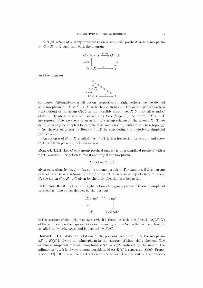
ON MOTIVIC SPHERICAL BUNDLES 45
A (left) action of a group presheaf G on a simplicial presheaf X is a morphism
α : G×X → X such that both the diagram
G×G×X id×α//
m×id
G×X
α
G×X α // X
and the diagram
X
∗ ×Xe×id
G×X α // X
commute. Alternatively, a left action (respectively a right action) may be defined
as a morphism α : G × X → X such that α induces a left action (respectively a
right action) of the group G(U) on the (possibly empty) set X(U)n for all n and U
of SmS . By abuse of notation, we write gx for α(U)(g, x)n. As above, if G and X
are representable, we speak of an action of a group scheme on the scheme X. These
definitions may be adopted for simplicial sheaves on SmS with respect to a topology
τ (or sheaves on k -Alg by Remark 1.0.2) by considering the underlying simplicial
presheaves.
An action α of G on X is called free, if α(U)n is a free action for every n and every
U , this is from gx = hx, it follows g = h.
Remark 3.1.2. Let G be a group presheaf and let E be a simplicial presheaf with a
right G-action. The action is free if and only if the morphism
E ×G→ E × E
given on sections by (x, g) 7→ (x, xg) is a monomorphism. For example, if G is a group
presheaf and H is a subgroup presheaf, id est H(U) is a subgroup of G(U) for every
U , the action G×H → G given by the multiplication is a free action.
Definition 3.1.3. Let α be a right action of a group presheaf G on a simplicial
presheaf E. The object defined by the pushout
aE × aG aα //
pr
aE
aE // aE/aG
in the category of simplicial τ -sheaves (which is the same as the sheafification aτ (E/X)
of the simplicial presheaf quotient) viewed as an object of sPre via the inclusion functor
is called the τ -orbit space and is denoted by E//τG.
Remark 3.1.4. With the notations of the previous Definition 3.1.3, the morphism
aE → E//τG is always an epimorphism in the category of simplicial τ -sheaves. The
canonical simplicial presheaf morphism E/G → E//τG induced by the unit of the
adjunction (aτ , i) is always a monomorphism, id est E/G is separated [Skj09, Propo-
sition 1.13]. If α is a free right action of aG on aE, the pushout of the previous

46 FLORIAN STRUNK
Definition 3.1.3 is also a pullback as the monomorphism aE × aG aE × aE defines
an equivalence relation [MM92, Theorem Appendix.1.1] and there is an isomorphism
aE × aG∼=−→ aE ×E//τG
aE
of simplicial presheaves (we omit the inclusion functor i by abuse of notation).
Remark 3.1.5. The existence of the isomorphism in the previous Remark 3.1.4 does
not imply that the orbit space E//τG with respect to a topology τ coincides with the
orbit space in another topology [Skj09, Lemma 3.6]. It is an interesting and non-trivial
question to decide whether a quotient E//τG with respect to a certain Grothendieck
topology is actually representable by an object of SmS . There are more tools available
to decide this question, the finer the topology is and the subcanonical fppf topology
which is even finer than the etale topology turns out to be helpful (confer [DG70,
Chapitre III] or [Jan87]). If an orbit space E//τG is a simplicial sheaf in a finer topology
τ ′, one has E//τG ∼= E//
τ’G as simplicial presheaves by definition. In particular, if the
orbit space E//τG is representable by an object of SmS , it is the orbit space for any
finer topology τ ′.
Remark 3.1.6. We briefly recall some definitions and statements of category and
topos theory. If C is complete category, a regular monomorphism, is a morphism
f : A→ B which fits into an equalizer diagram
Af−→ B ⇒ C
whereas a monomorphism f : A→ B just fits into a a pullback diagram
A A
f
A //f// B.
For a cocomplete category, a regular epimorphism is defined analogously. A regular
monomorphism is in particular a monomorphism. The analogous statement holds for
epimorphisms.
From Giraud’s theorem [MM92, Theorem Appendix.1.1], one deduces that every
topos is complete and cocomplete [Bor94c, Proposition 3.4.3], every monomorphism
is a regular monomorphism [Bor94c, Proposition 3.4.11] and every epimorphism is a
regular epimorphism [Bor94c, Proposition 3.4.13].
Let C be a complete and cocomplete category.
(1) A pullback of a monomorphism is a monomorphism and a pushout of an
epimorphism is an epimorphism.
(2) If C is a topos, a pushout of a monomorphism is a monomorphism and a
pullback of an epimorphism is an epimorphism [LS06, Lemma 18].
(3) If the the solid diagram
A //
B
Q
??
C // P
is a pushout, then the pullback diagram Q-B-C-P is also a pushout diagram.
The dual statement holds as well.
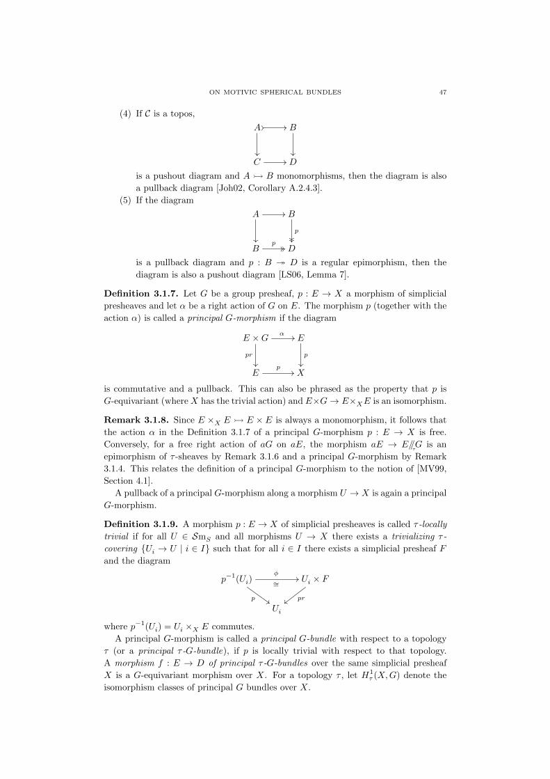
ON MOTIVIC SPHERICAL BUNDLES 47
(4) If C is a topos,
A
// // B
C // D
is a pushout diagram and A B monomorphisms, then the diagram is also
a pullback diagram [Joh02, Corollary A.2.4.3].
(5) If the diagram
A
// B
p
Bp// // D
is a pullback diagram and p : B D is a regular epimorphism, then the
diagram is also a pushout diagram [LS06, Lemma 7].
Definition 3.1.7. Let G be a group presheaf, p : E → X a morphism of simplicial
presheaves and let α be a right action of G on E. The morphism p (together with the
action α) is called a principal G-morphism if the diagram
E ×G α //
pr
E
p
Ep// X
is commutative and a pullback. This can also be phrased as the property that p is
G-equivariant (where X has the trivial action) and E×G→ E×XE is an isomorphism.
Remark 3.1.8. Since E ×X E E × E is always a monomorphism, it follows that
the action α in the Definition 3.1.7 of a principal G-morphism p : E → X is free.
Conversely, for a free right action of aG on aE, the morphism aE → E//τG is an
epimorphism of τ -sheaves by Remark 3.1.6 and a principal G-morphism by Remark
3.1.4. This relates the definition of a principal G-morphism to the notion of [MV99,
Section 4.1].
A pullback of a principal G-morphism along a morphism U → X is again a principal
G-morphism.
Definition 3.1.9. A morphism p : E → X of simplicial presheaves is called τ -locally
trivial if for all U ∈ SmS and all morphisms U → X there exists a trivializing τ -
covering Ui → U | i ∈ I such that for all i ∈ I there exists a simplicial presheaf F
and the diagram
p−1(Ui)
p##
φ
∼=// Ui × F
pr
Ui
where p−1(Ui) = Ui ×X E commutes.
A principal G-morphism is called a principal G-bundle with respect to a topology
τ (or a principal τ -G-bundle), if p is locally trivial with respect to that topology.
A morphism f : E → D of principal τ -G-bundles over the same simplicial presheaf
X is a G-equivariant morphism over X. For a topology τ , let H1τ (X,G) denote the
isomorphism classes of principal G bundles over X.
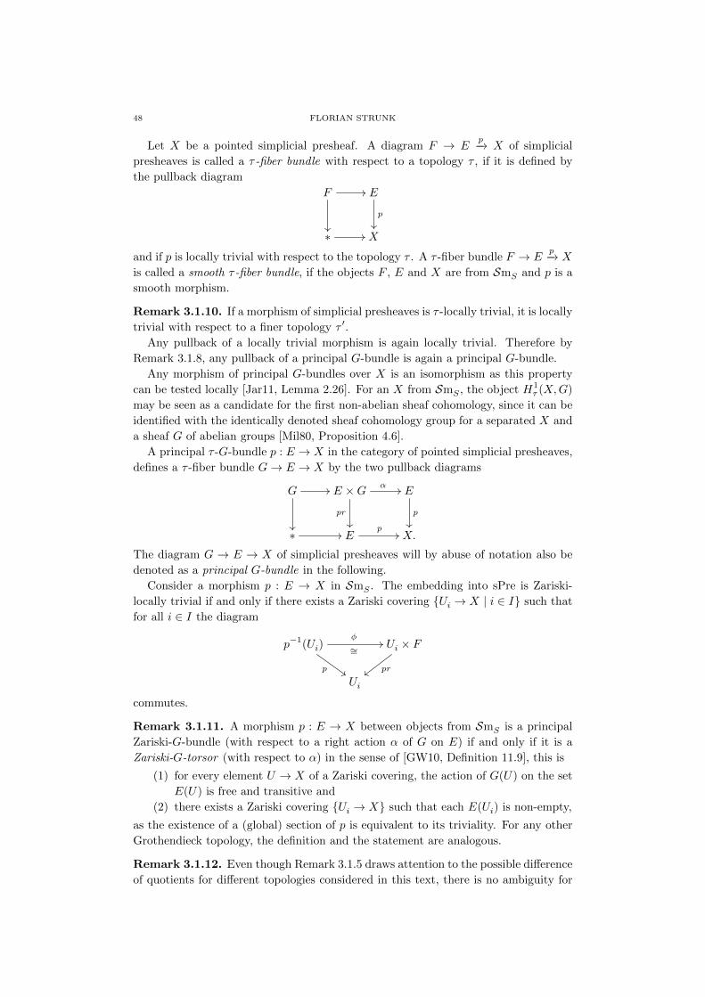
48 FLORIAN STRUNK
Let X be a pointed simplicial presheaf. A diagram F → Ep−→ X of simplicial
presheaves is called a τ -fiber bundle with respect to a topology τ , if it is defined by
the pullback diagram
F //
E
p
∗ // X
and if p is locally trivial with respect to the topology τ . A τ -fiber bundle F → Ep−→ X
is called a smooth τ -fiber bundle, if the objects F , E and X are from SmS and p is a
smooth morphism.
Remark 3.1.10. If a morphism of simplicial presheaves is τ -locally trivial, it is locally
trivial with respect to a finer topology τ ′.
Any pullback of a locally trivial morphism is again locally trivial. Therefore by
Remark 3.1.8, any pullback of a principal G-bundle is again a principal G-bundle.
Any morphism of principal G-bundles over X is an isomorphism as this property
can be tested locally [Jar11, Lemma 2.26]. For an X from SmS , the object H1τ (X,G)
may be seen as a candidate for the first non-abelian sheaf cohomology, since it can be
identified with the identically denoted sheaf cohomology group for a separated X and
a sheaf G of abelian groups [Mil80, Proposition 4.6].
A principal τ -G-bundle p : E → X in the category of pointed simplicial presheaves,
defines a τ -fiber bundle G→ E → X by the two pullback diagrams
G //
E ×G α //
pr
E
p
∗ // Ep// X.
The diagram G → E → X of simplicial presheaves will by abuse of notation also be
denoted as a principal G-bundle in the following.
Consider a morphism p : E → X in SmS . The embedding into sPre is Zariski-
locally trivial if and only if there exists a Zariski covering Ui → X | i ∈ I such that
for all i ∈ I the diagram
p−1(Ui)
p##
φ
∼=// Ui × F
pr
Ui
commutes.
Remark 3.1.11. A morphism p : E → X between objects from SmS is a principal
Zariski-G-bundle (with respect to a right action α of G on E) if and only if it is a
Zariski-G-torsor (with respect to α) in the sense of [GW10, Definition 11.9], this is
(1) for every element U → X of a Zariski covering, the action of G(U) on the set
E(U) is free and transitive and
(2) there exists a Zariski covering Ui → X such that each E(Ui) is non-empty,
as the existence of a (global) section of p is equivalent to its triviality. For any other
Grothendieck topology, the definition and the statement are analogous.
Remark 3.1.12. Even though Remark 3.1.5 draws attention to the possible difference
of quotients for different topologies considered in this text, there is no ambiguity for

ON MOTIVIC SPHERICAL BUNDLES 49
a Zariski-locally trivial situation: Consider a topology τ ′ finer than a topology τ , and
let α be a free right action of a group presheaf G from SmS on a simplicial presheaf
E from SmS . The pushout
E ×G aα //
pr
E
p
E // E//τ’G
defines the quotient in the category of simplicial τ ′-sheaves. If the epimorphism p is
τ -locally trivial, it is an epimorphism in the category of simplicial τ -sheaves as well as
a projection is always an epimorphism and those are detected locally [Jar11, Lemma
2.26]. By Remark 3.1.6, the diagram is then a pushout in the category of simplicial
τ -sheaves which implies that the quotients (viewed as simplicial presheaves) coincide
by Remark 3.1.5.
Remark 3.1.13. A Grothendieck pre-topology Cov on a complete category C defines
a Grothendieck pre-topology Cov where
Cov(X) = Ui → X | Ui → X is refined by some element in Cov(X)
called the saturation of Cov. If two Grothendieck pre-topologies refine each other,
they have the same saturation. Even though for every covering Ui → X of a pre-
topology Cov on C, the morphism∐ayUi ayX is an epimorphism of Shv(C), the
converse may not be true. However, a morphism∐i
ayUi → ayX
is an epimorphism of Shv(C) if and only if Ui → X is an element of Cov(X) [MM92,
Corollary III.7.7].
Lemma 3.1.14. In the category sShv of simplicial sheaves with respect to a
topology τ , a principal G-morphism p : E → X between objects from SmS is
τ -locally trivial if and only if it is an epimorphism.
Proof. A locally trivial morphism is an epimorphism in the category of simplicial
sheaves as the projection out of a product is an epimorphism and being an epimorphism
is a local property by [Jar11, Lemma 2.26].
For the other implication, let p : E → X be a principal G-morphism of objects
from SmS which is an epimorphism. Consider the diagram
E ×G∼= //
pr%%
E ×X E
// E
p
Ep// // X
and pick a τ -covering Ui → E of E. Since by Remark 3.1.13, the map∐Ui → E is
an epimorphism of τ -sheaves, so is the composition∐Ui → E → X. Then, Remark
3.1.13 implies, that Ui → X is a covering of X in the saturation of the pre-topology
τ . Hence, it is refined by some τ -covering Ui → X of X, which we denote likewise,
by abuse of notation. All in all, there is a τ -covering Ui → X of X, such that each
Ui → X factorizes through p : E → X.

50 FLORIAN STRUNK
Pulling back along Ui → X defines the diagram
E ×Gxx
∼= // E ×X E
// E
p
Ui ×G∼= //
''
p−1(Ui)
77
((E
p// // X
Ui
66
which implies the result.
Definition 3.1.15. Let α be a free right action of a group presheaf G on a simplicial
presheaf E. Let β be a (not necessarily free) left action of G on a simplicial presheaf
F . The morphism
(E × F )×G→ E × Fgiven on sections by (e, f, g) 7→ (eg, g−1f) defines a free right action on E × F whose
orbit space (E × F )//τG with respect to a topology τ is denoted by E×GF (ignoring
the topology τ in the notation). The diagram
E × F ×G //
prww
E × F
prwwE ×G
//
E
E × Fpr
xx
// (E × F )//τG
p×GFxx
E // E//τG
provides a canonical morphism p×GF : E×GF → E//τG.
Lemma 3.1.16. Let G be a τ -group sheaf and let F be a simplicial τ -sheaf. Let
G → Ep−→ X be a principal τ -G-bundle, E and X be objects from SmS and let
F be equipped with a left G-action. Then
F → E×GF p×GF−−−−→ X
is a τ -fiber bundle.
Moreover, if F is a group sheaf and ϕ : G → F a group homomorphism (id
est a homomorphism for each section) through which G acts on F from the left,
then the above fiber bundle is a principal τ -F -bundle where F acts on E×GFfrom the right by (the sheafification of) [e, f ]f ′ = [e, ff ′].
Proof. Since p is a principal τ -G-bundle, one has X ∼= E//τG. The bottom diagram
E × F //
(E × F )/G
E // E/G
of the cube in Definition 3.1.15 with quotients taken in the category of simplicial
presheaves is a pullback, since it is a pullback in each simplicial degree and in every
section (confer [Jan87, 5.14.3]). The sheafification functor with respect to the topology
τ commutes with pullbacks and thus the diagram of the associated sheaves is a pullback
as well.

ON MOTIVIC SPHERICAL BUNDLES 51
With the same reasoning as in the proof of Lemma 3.1.14, there is a τ -covering
Ui → X factorizing through p. Hence, the pullback diagram
Ui × F //
E × F //
(E × F )//τG
p×GF
Ui// E
p// // E//
τG
implies that p×GF is τ -locally trivial and F → E×GF → X is a τ -fiber bundle.
If F group sheaf, the above-mentioned action of F on E×GF is well defined and
free which may be tested section-wise: From [e, f ]f ′ = [e, f ], which means that there
exists a g such that (eg, ϕ(g−1)ff ′) = (e, f), it follows that f ′ is the unit element
because F acts freely on itself. Since the action of G on E × F commutes with the
action of F on E×F , applying the sheafification functor with respect to the topology
τ yields (E×GF )//τF ∼= E//
τG ∼= X (confer [Jan87, I.5.18]).
Definition 3.1.17. In the situation of Lemma 3.1.16, on says that
F → E×GF p×GF−−−−→ X
is an extension of the structure group of
G→ Ep−→ X
by ϕ : G→ F . Conversely, p is a reduction of the structure group of p×GF by ϕ.
Lemma 3.1.18 ([Jan87, I.5.16.1]). Let G be a Zariski-group sheaf, G→ E → X
be a principal Zariski-G-bundle, F , E and X be from SmS and let F be equipped
with a left G-action. Then E×GF comes from SmS .
Lemma 3.1.19. Let G be a τ -group sheaf, ϕ : H → G a τ -subgroup sheaf.
Let moreover E and X be objects from SmS and G → Ep−→ X be a principal
τ -G-bundle. Then, there exists a pullback diagram
E×HG //
q×HG
E
p
G//τH // E//
τH
f// X
of simplicial presheaves, where the lower horizontal morphisms constitute a τ -
fiber bundle and where q×HG is the extension of the structure group of the
canonical principal τ -H-bundle q : E → E//τH.
Proof. Equip G//τH with the canonical left G-action given on simplicial presheaves by
G×G/H → G/H by g′(gH) = g′gH. Lemma 3.1.16 provides a τ -fiber bundle
G//τH → E×G(G//
τH)
f−→ X.
A free right action on E×G by G×H is given by (e, g)(g′, h) = (eg′, g′−1gh). The two
induced actions by G and H on E ×G respectively commute and hence the quotient
(E ×G)/(G×H) may be taken successively. This shows (E ×G/H)/G ∼= E/H and
f is identified with the canonical map E//τH → E//
τG ∼= X after sheafification. Hence,
there is a τ -fiber bundle
G//τH → E//
τH
f−→ X.

52 FLORIAN STRUNK
As the action E × Hid×ϕ−−−→ E × G → E of H on E is free, it defines a principal
τ -H-bundle q : E → E//τH. We have to show, that q×HG is the pullback of f and p
because this implies already that it is τ -locally trivial. The diagram
(E ×G)/H //
(E ×G)/G
E/H // E/G
of simplicial presheaves is a pullback and hence its sheafification is a pullback as well.
This implies the result.
Lemma 3.1.20. If in the situation of the above Lemma 3.1.19, the topology τ
is the Zariski topology and if G//τH is an object from SmS , then also E//
τH is an
object from SmS .
Proof. This follows from the isomorphism E×G(G//τH) ∼= E//
τH of the previous Lemma
3.1.19 and Lemma 3.1.18.
3.2. Fiber sequences from bundles
We assume the base scheme S to be the spectrum of a field k for the whole section.
Lemma 3.2.1. For pointed simplicial presheaves X and F where X is from SmS ,
a Zariski-fiber bundle F → Ep−→ X defines a local fiber sequence.
Proof. This is either implied by Theorem 1.2.11 considering stalks or differently by
[Rez98, Theorem 5.1]: By (P4), p is locally sharp if the base change along the epi-
morphism∐Ui → X for a trivializing Zariski-covering Ui → X is locally sharp. By
(P5), a coproduct of locally sharp maps is again sharp and hence it suffices to show
that the projections Ui × F → Ui are locally sharp. By (P2), the morphism F → ∗is locally sharp and hence the projections are locally sharp as sharp morphisms are
stable under basechange by Remark 1.2.10.
Remark 3.2.2. Of course, the previous Lemma 3.2.1 requires the bundle F → E → X
only to be Nisnevich-locally trivial. It is observed in [Wen07, Proposition 3.3.7], that
even an etale-fiber bundle of objects from SmS induces a local fiber sequence.
Remark 3.2.3. We are interested in the fact whether certain Zariski-fiber bundles
F → E → X induce motivic fiber sequences. By Corollary 1.2.15, this is for example
the case if X is an A1-local scheme. As X → Sing(X) is a motivic weak equivalence
and the singular functor of Remark 1.1.21 commutes with pullbacks, one may as well
ask if Sing(F ) → Sing(E) → Sing(X) is a motivic fiber sequence because this pre-
fiber sequence belongs to the same equivalence class as F → E → X.
Definition 3.2.4. For an integer n ≥ 1, one sets
GLn = Spec k[x11, . . . , xij , . . . , xnn, t]/(det(xij)t− 1)
as the general linear group scheme over S. This is a group object of SmS by means
of the canonical Hopf algebra structure given by the comultiplication ∆ defined by
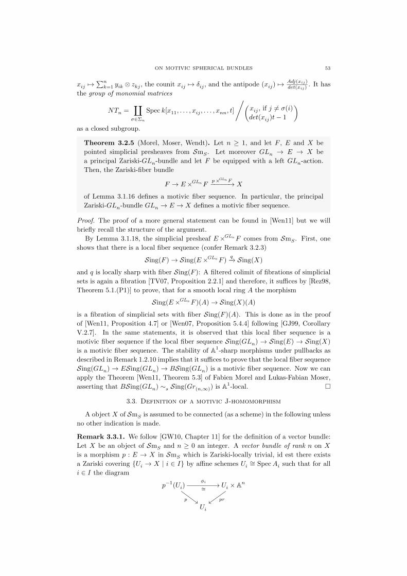
ON MOTIVIC SPHERICAL BUNDLES 53
xij 7→∑nk=1 yik ⊗ zkj , the counit xij 7→ δij , and the antipode (xij) 7→
Adj(xij)det(xij)
. It has
the group of monomial matrices
NTn =∐σ∈Σn
Spec k[x11, . . . , xij , . . . , xnn, t]
/(xij , if j 6= σ(i)
det(xij)t− 1
)as a closed subgroup.
Theorem 3.2.5 (Morel, Moser, Wendt). Let n ≥ 1, and let F , E and X be
pointed simplicial presheaves from SmS . Let moreover GLn → E → X be
a principal Zariski-GLn-bundle and let F be equipped with a left GLn-action.
Then, the Zariski-fiber bundle
F → E×GLn Fp×GLn F−−−−−→ X
of Lemma 3.1.16 defines a motivic fiber sequence. In particular, the principal
Zariski-GLn-bundle GLn → E → X defines a motivic fiber sequence.
Proof. The proof of a more general statement can be found in [Wen11] but we will
briefly recall the structure of the argument.
By Lemma 3.1.18, the simplicial presheaf E×GLn F comes from SmS . First, one
shows that there is a local fiber sequence (confer Remark 3.2.3)
Sing(F )→ Sing(E×GLn F )q−→ Sing(X)
and q is locally sharp with fiber Sing(F ): A filtered colimit of fibrations of simplicial
sets is again a fibration [TV07, Proposition 2.2.1] and therefore, it suffices by [Rez98,
Theorem 5.1.(P1)] to prove, that for a smooth local ring A the morphism
Sing(E×GLn F )(A)→ Sing(X)(A)
is a fibration of simplicial sets with fiber Sing(F )(A). This is done as in the proof
of [Wen11, Proposition 4.7] or [Wen07, Proposition 5.4.4] following [GJ99, Corollary
V.2.7]. In the same statements, it is observed that this local fiber sequence is a
motivic fiber sequence if the local fiber sequence Sing(GLn) → Sing(E) → Sing(X)
is a motivic fiber sequence. The stability of A1-sharp morphisms under pullbacks as
described in Remark 1.2.10 implies that it suffices to prove that the local fiber sequence
Sing(GLn)→ ESing(GLn)→ BSing(GLn) is a motivic fiber sequence. Now we can
apply the Theorem [Wen11, Theorem 5.3] of Fabien Morel and Lukas-Fabian Moser,
asserting that BSing(GLn) ∼s Sing(Gr(n,∞)) is A1-local.
3.3. Definition of a motivic J-homomorphism
A object X of SmS is assumed to be connected (as a scheme) in the following unless
no other indication is made.
Remark 3.3.1. We follow [GW10, Chapter 11] for the definition of a vector bundle:
Let X be an object of SmS and n ≥ 0 an integer. A vector bundle of rank n on X
is a morphism p : E → X in SmS which is Zariski-locally trivial, id est there exists
a Zariski covering Ui → X | i ∈ I by affine schemes Ui∼= SpecAi such that for all
i ∈ I the diagram
p−1(Ui)
p##
φi
∼=// Ui × An
pr
Ui
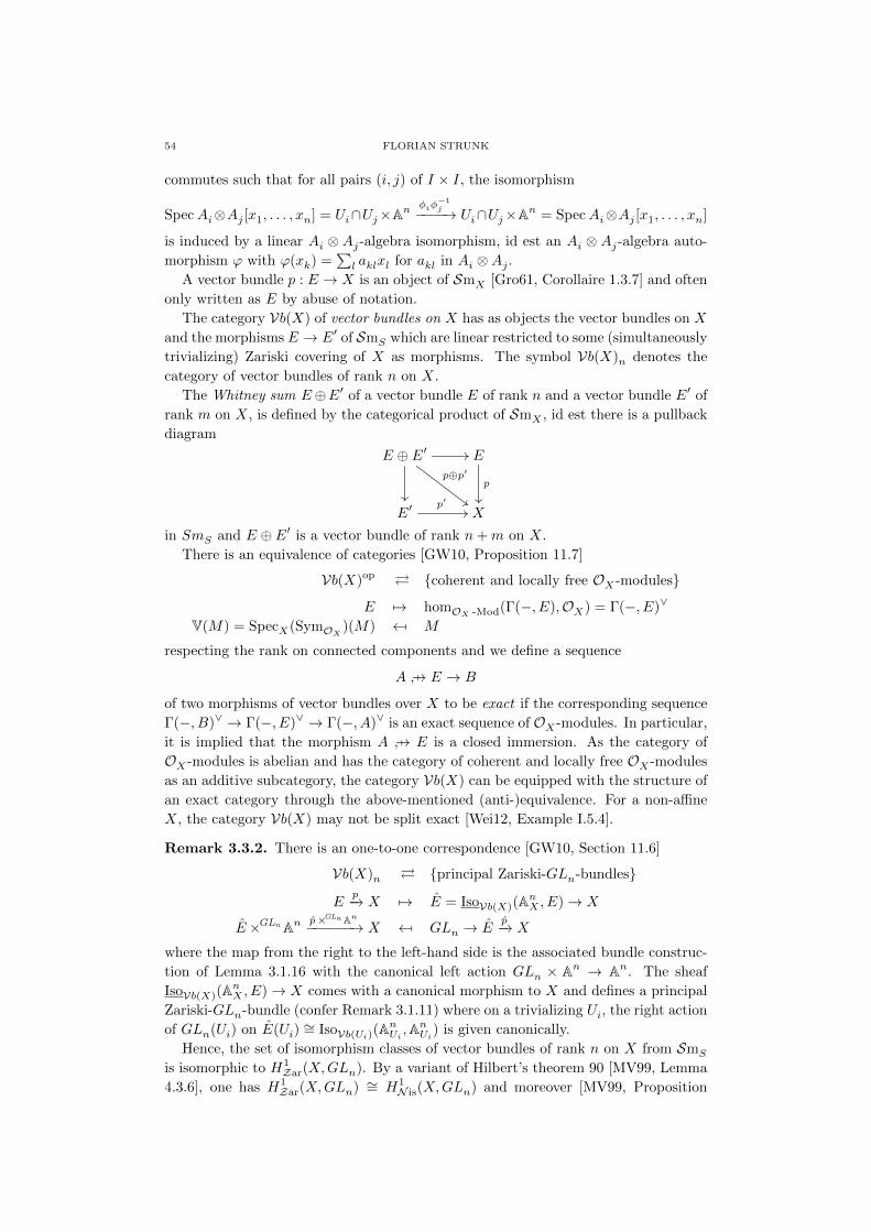
54 FLORIAN STRUNK
commutes such that for all pairs (i, j) of I × I, the isomorphism
SpecAi⊗Aj [x1, . . . , xn] = Ui∩Uj×An
φiφ−1j−−−−→ Ui∩Uj×A
n = SpecAi⊗Aj [x1, . . . , xn]
is induced by a linear Ai ⊗ Aj-algebra isomorphism, id est an Ai ⊗ Aj-algebra auto-
morphism ϕ with ϕ(xk) =∑l aklxl for akl in Ai ⊗Aj .
A vector bundle p : E → X is an object of SmX [Gro61, Corollaire 1.3.7] and often
only written as E by abuse of notation.
The category Vb(X) of vector bundles on X has as objects the vector bundles on X
and the morphisms E → E′ of SmS which are linear restricted to some (simultaneously
trivializing) Zariski covering of X as morphisms. The symbol Vb(X)n denotes the
category of vector bundles of rank n on X.
The Whitney sum E⊕E′ of a vector bundle E of rank n and a vector bundle E′ of
rank m on X, is defined by the categorical product of SmX , id est there is a pullback
diagram
E ⊕ E′ //
p⊕p′
##
E
p
E′p′
// X
in SmS and E ⊕ E′ is a vector bundle of rank n+m on X.
There is an equivalence of categories [GW10, Proposition 11.7]
Vb(X)op coherent and locally free OX -modules
E 7→ homOX -Mod(Γ(−, E),OX) = Γ(−, E)∨
V(M) = SpecX(SymOX )(M) ←[ M
respecting the rank on connected components and we define a sequence
A →[ E → B
of two morphisms of vector bundles over X to be exact if the corresponding sequence
Γ(−, B)∨ → Γ(−, E)∨ → Γ(−, A)∨ is an exact sequence of OX -modules. In particular,
it is implied that the morphism A →[ E is a closed immersion. As the category of
OX -modules is abelian and has the category of coherent and locally free OX -modules
as an additive subcategory, the category Vb(X) can be equipped with the structure of
an exact category through the above-mentioned (anti-)equivalence. For a non-affine
X, the category Vb(X) may not be split exact [Wei12, Example I.5.4].
Remark 3.3.2. There is an one-to-one correspondence [GW10, Section 11.6]
Vb(X)n principal Zariski-GLn-bundles
Ep−→ X 7→ E = IsoVb(X)(A
nX , E)→ X
E×GLn An p×GLn An−−−−−−→ X ← [ GLn → Ep−→ X
where the map from the right to the left-hand side is the associated bundle construc-
tion of Lemma 3.1.16 with the canonical left action GLn × An → An. The sheaf
IsoVb(X)(AnX , E)→ X comes with a canonical morphism to X and defines a principal
Zariski-GLn-bundle (confer Remark 3.1.11) where on a trivializing Ui, the right action
of GLn(Ui) on E(Ui)∼= IsoVb(Ui)(A
nUi,AnUi) is given canonically.
Hence, the set of isomorphism classes of vector bundles of rank n on X from SmS
is isomorphic to H1Zar(X,GLn). By a variant of Hilbert’s theorem 90 [MV99, Lemma
4.3.6], one has H1Zar(X,GLn) ∼= H1
N is(X,GLn) and moreover [MV99, Proposition
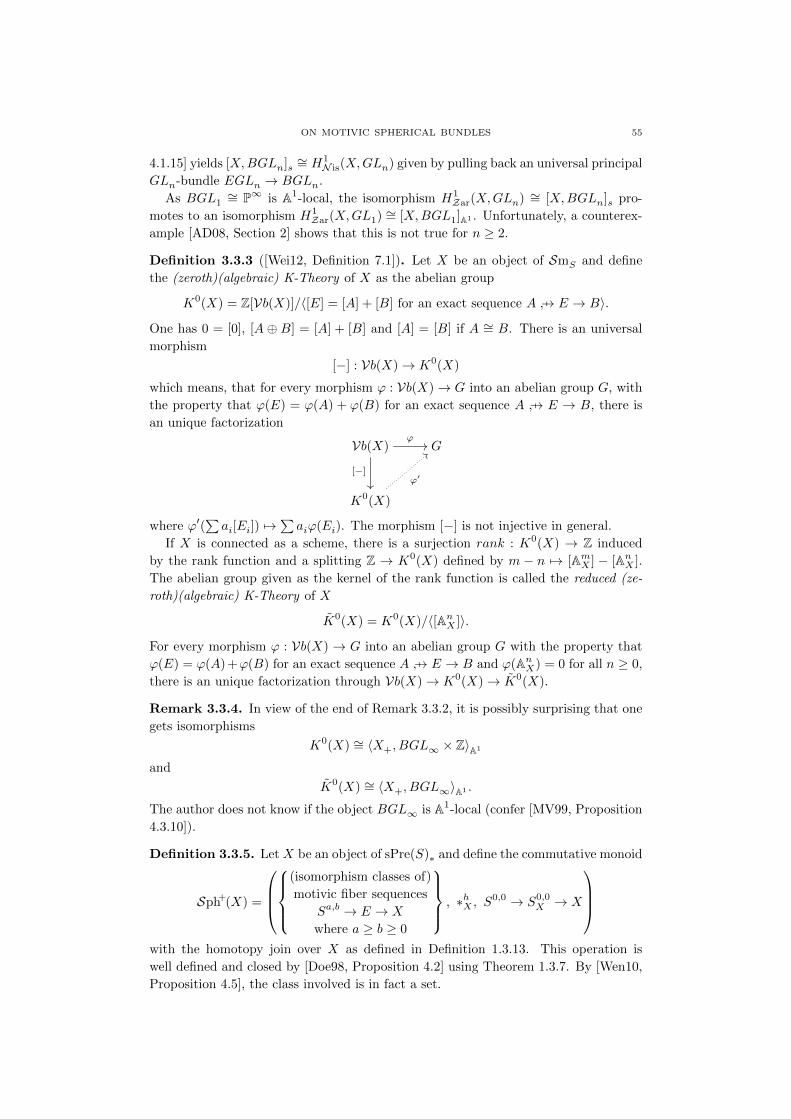
ON MOTIVIC SPHERICAL BUNDLES 55
4.1.15] yields [X,BGLn]s∼= H1
N is(X,GLn) given by pulling back an universal principal
GLn-bundle EGLn → BGLn.
As BGL1∼= P∞ is A1-local, the isomorphism H1
Zar(X,GLn) ∼= [X,BGLn]s pro-
motes to an isomorphism H1Zar(X,GL1) ∼= [X,BGL1]A1 . Unfortunately, a counterex-
ample [AD08, Section 2] shows that this is not true for n ≥ 2.
Definition 3.3.3 ([Wei12, Definition 7.1]). Let X be an object of SmS and define
the (zeroth)(algebraic) K-Theory of X as the abelian group
K0(X) = Z[Vb(X)]/〈[E] = [A] + [B] for an exact sequence A →[ E → B〉.
One has 0 = [0], [A ⊕ B] = [A] + [B] and [A] = [B] if A ∼= B. There is an universal
morphism
[−] : Vb(X)→ K0(X)
which means, that for every morphism ϕ : Vb(X)→ G into an abelian group G, with
the property that ϕ(E) = ϕ(A) + ϕ(B) for an exact sequence A →[ E → B, there is
an unique factorization
Vb(X)ϕ//
[−]
G
K0(X)
ϕ′
<<
where ϕ′(∑ai[Ei]) 7→
∑aiϕ(Ei). The morphism [−] is not injective in general.
If X is connected as a scheme, there is a surjection rank : K0(X) → Z induced
by the rank function and a splitting Z → K0(X) defined by m − n 7→ [AmX ] − [AnX ].
The abelian group given as the kernel of the rank function is called the reduced (ze-
roth)(algebraic) K-Theory of X
K0(X) = K0(X)/〈[AnX ]〉.
For every morphism ϕ : Vb(X) → G into an abelian group G with the property that
ϕ(E) = ϕ(A)+ϕ(B) for an exact sequence A →[ E → B and ϕ(AnX) = 0 for all n ≥ 0,
there is an unique factorization through Vb(X)→ K0(X)→ K0(X).
Remark 3.3.4. In view of the end of Remark 3.3.2, it is possibly surprising that one
gets isomorphisms
K0(X) ∼= 〈X+, BGL∞ × Z〉A1
and
K0(X) ∼= 〈X+, BGL∞〉A1 .
The author does not know if the object BGL∞ is A1-local (confer [MV99, Proposition
4.3.10]).
Definition 3.3.5. Let X be an object of sPre(S)∗ and define the commutative monoid
Sph+(X) =
(isomorphism classes of)
motivic fiber sequences
Sa,b → E → X
where a ≥ b ≥ 0
, ∗hX , S0,0 → S0,0
X → X
with the homotopy join over X as defined in Definition 1.3.13. This operation is
well defined and closed by [Doe98, Proposition 4.2] using Theorem 1.3.7. By [Wen10,
Proposition 4.5], the class involved is in fact a set.
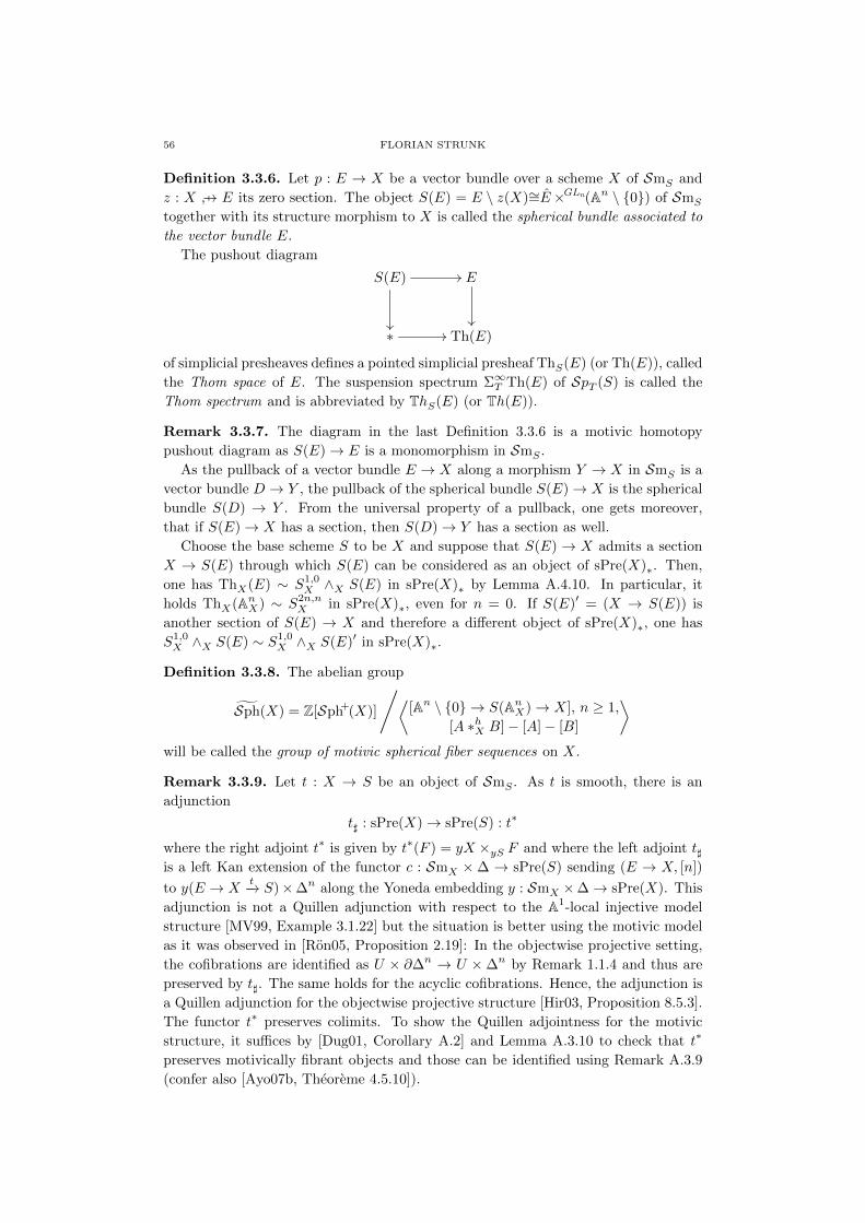
56 FLORIAN STRUNK
Definition 3.3.6. Let p : E → X be a vector bundle over a scheme X of SmS and
z : X →[ E its zero section. The object S(E) = E \ z(X)∼=E×GLn(An \ 0) of SmS
together with its structure morphism to X is called the spherical bundle associated to
the vector bundle E.
The pushout diagram
S(E) //
E
∗ // Th(E)
of simplicial presheaves defines a pointed simplicial presheaf ThS(E) (or Th(E)), called
the Thom space of E. The suspension spectrum Σ∞T Th(E) of SpT (S) is called the
Thom spectrum and is abbreviated by ThS(E) (or Th(E)).
Remark 3.3.7. The diagram in the last Definition 3.3.6 is a motivic homotopy
pushout diagram as S(E)→ E is a monomorphism in SmS .
As the pullback of a vector bundle E → X along a morphism Y → X in SmS is a
vector bundle D → Y , the pullback of the spherical bundle S(E)→ X is the spherical
bundle S(D) → Y . From the universal property of a pullback, one gets moreover,
that if S(E)→ X has a section, then S(D)→ Y has a section as well.
Choose the base scheme S to be X and suppose that S(E) → X admits a section
X → S(E) through which S(E) can be considered as an object of sPre(X)∗. Then,
one has ThX(E) ∼ S1,0X ∧X S(E) in sPre(X)∗ by Lemma A.4.10. In particular, it
holds ThX(AnX) ∼ S2n,nX in sPre(X)∗, even for n = 0. If S(E)′ = (X → S(E)) is
another section of S(E) → X and therefore a different object of sPre(X)∗, one has
S1,0X ∧X S(E) ∼ S1,0
X ∧X S(E)′ in sPre(X)∗.
Definition 3.3.8. The abelian group
Sph(X) = Z[Sph+(X)]
/⟨[An \ 0 → S(AnX)→ X], n ≥ 1,
[A ∗hX B]− [A]− [B]
⟩will be called the group of motivic spherical fiber sequences on X.
Remark 3.3.9. Let t : X → S be an object of SmS . As t is smooth, there is an
adjunction
t] : sPre(X)→ sPre(S) : t∗
where the right adjoint t∗ is given by t∗(F ) = yX ×yS F and where the left adjoint t]is a left Kan extension of the functor c : SmX ×∆ → sPre(S) sending (E → X, [n])
to y(E → Xt−→ S)×∆n along the Yoneda embedding y : SmX ×∆→ sPre(X). This
adjunction is not a Quillen adjunction with respect to the A1-local injective model
structure [MV99, Example 3.1.22] but the situation is better using the motivic model
as it was observed in [Ron05, Proposition 2.19]: In the objectwise projective setting,
the cofibrations are identified as U × ∂∆n → U ×∆n by Remark 1.1.4 and thus are
preserved by t]. The same holds for the acyclic cofibrations. Hence, the adjunction is
a Quillen adjunction for the objectwise projective structure [Hir03, Proposition 8.5.3].
The functor t∗ preserves colimits. To show the Quillen adjointness for the motivic
structure, it suffices by [Dug01, Corollary A.2] and Lemma A.3.10 to check that t∗
preserves motivically fibrant objects and those can be identified using Remark A.3.9
(confer also [Ayo07b, Theoreme 4.5.10]).
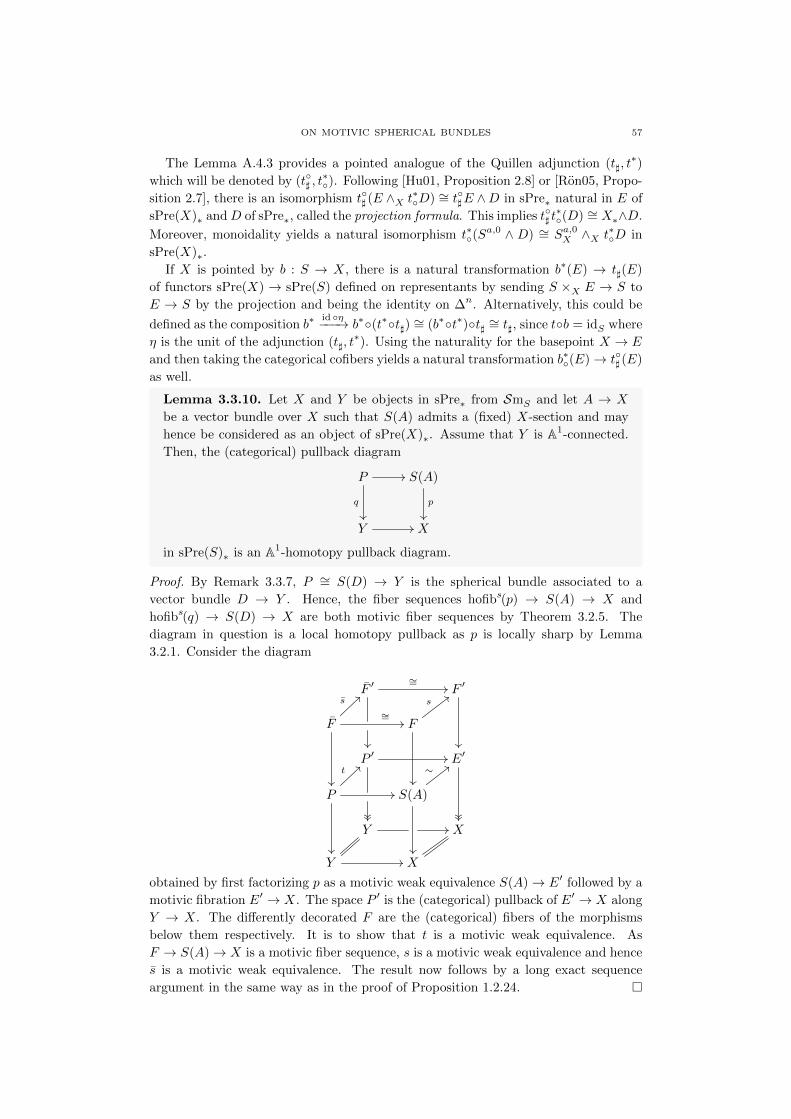
ON MOTIVIC SPHERICAL BUNDLES 57
The Lemma A.4.3 provides a pointed analogue of the Quillen adjunction (t], t∗)
which will be denoted by (t] , t∗). Following [Hu01, Proposition 2.8] or [Ron05, Propo-
sition 2.7], there is an isomorphism t] (E ∧X t∗D) ∼= t]E ∧D in sPre∗ natural in E of
sPre(X)∗ andD of sPre∗, called the projection formula. This implies t] t∗(D) ∼= X∗∧D.
Moreover, monoidality yields a natural isomorphism t∗(Sa,0 ∧ D) ∼= Sa,0X ∧X t∗D in
sPre(X)∗.
If X is pointed by b : S → X, there is a natural transformation b∗(E) → t](E)
of functors sPre(X) → sPre(S) defined on representants by sending S ×X E → S to
E → S by the projection and being the identity on ∆n. Alternatively, this could be
defined as the composition b∗id η−−−→ b∗(t∗t]) ∼= (b∗t∗)t] ∼= t], since tb = idS where
η is the unit of the adjunction (t], t∗). Using the naturality for the basepoint X → E
and then taking the categorical cofibers yields a natural transformation b∗(E)→ t] (E)
as well.
Lemma 3.3.10. Let X and Y be objects in sPre∗ from SmS and let A → X
be a vector bundle over X such that S(A) admits a (fixed) X-section and may
hence be considered as an object of sPre(X)∗. Assume that Y is A1-connected.
Then, the (categorical) pullback diagram
P //
q
S(A)
p
Y // X
in sPre(S)∗ is an A1-homotopy pullback diagram.
Proof. By Remark 3.3.7, P ∼= S(D) → Y is the spherical bundle associated to a
vector bundle D → Y . Hence, the fiber sequences hofibs(p) → S(A) → X and
hofibs(q) → S(D) → X are both motivic fiber sequences by Theorem 3.2.5. The
diagram in question is a local homotopy pullback as p is locally sharp by Lemma
3.2.1. Consider the diagram
F ′∼= //
>>s
F ′
;;s
F
∼= //
F
P ′ //??
tE′
<<∼
P
//
S(A)
Y // X
Y // X
obtained by first factorizing p as a motivic weak equivalence S(A)→ E′ followed by a
motivic fibration E′ → X. The space P ′ is the (categorical) pullback of E′ → X along
Y → X. The differently decorated F are the (categorical) fibers of the morphisms
below them respectively. It is to show that t is a motivic weak equivalence. As
F → S(A)→ X is a motivic fiber sequence, s is a motivic weak equivalence and hence
s is a motivic weak equivalence. The result now follows by a long exact sequence
argument in the same way as in the proof of Proposition 1.2.24.

58 FLORIAN STRUNK
Lemma 3.3.11. Let X be an object in sPre∗ from SmS and let A → X and
B → X be two vector bundles over X such that S(A) and S(B) admit a (fixed)
X-section and may hence be considered as objects of sPre(X)∗. Then, one has
S(A⊕B) ∼ S(A) ∧X S(B) ∧X S1,0X
in sPre(X)∗. If S(A) and S(B) are considered as objects of sPre∗ via the base-
point S → X, one has moreover
S(A⊕B) ∼ S(A) ∧hX S(B) ∧hX S1,0X
∼ S(A) ∗hX S(B)
in sPre∗ over X, if S(B) is A1-connected or if S(B) → X is a trivial spherical
bundle S(AnX)→ X with n ≥ 1.
Proof. The diagram
S(A) ∨X S(B) //
S(A) ∨X B
A ∨X S(B) // A ∨X B
is a homotopy pushout diagram in sPre(X)∗ as the functor −∨X − preserves pushout
diagrams in both variables and in a topos, the pushout of a monomorphism is a
monomorphism (confer Remark 3.1.6). The diagram
S(A)×X S(B) //
S(A)×X B
A×X S(B) // S(A⊕B)
is a Zariski distinguished square in SmX as the property of a diagram to be a pullback
in SmX is checked locally and there is a pullback diagram
Aa \ 0 × Ab \ 0 //
Aa \ 0 × Ab
Aa × Ab \ 0 // (Aa × Ab) \ 0.
Since a Zariski distinguished square defines a homotopy pushout for the local models
by Remark 1.1.13 and hence for the A1-local model structures, the categorical pushout
diagram
S(A) ∧X S(B) //
S(A) ∧X B
A ∧X S(B) // S(A⊕B)/A ∨X B
obtained by taking the cofibers of the morphism from the wedges to the products
respectively, is a motivic homotopy pushout diagram. As A ∨X B ∼ X in sPre(X)∗[Doe98, Lemma 1.4] and since the lower left corner and the upper right corner of this
homotopy pushout diagram are both weakly equivalent to X, one gets the relation
S(A⊕B) ∼ S(A) ∧X S(B) ∧X S1,0X in sPre(X)∗.
For the second assertion, one first notes that S(A) ∗hX S(B) is weakly equivalent
to S(A) ∧hX S(B) ∧hX S1,0X by Lemma 1.3.15 and the simplicial structure of sPre/X∗.
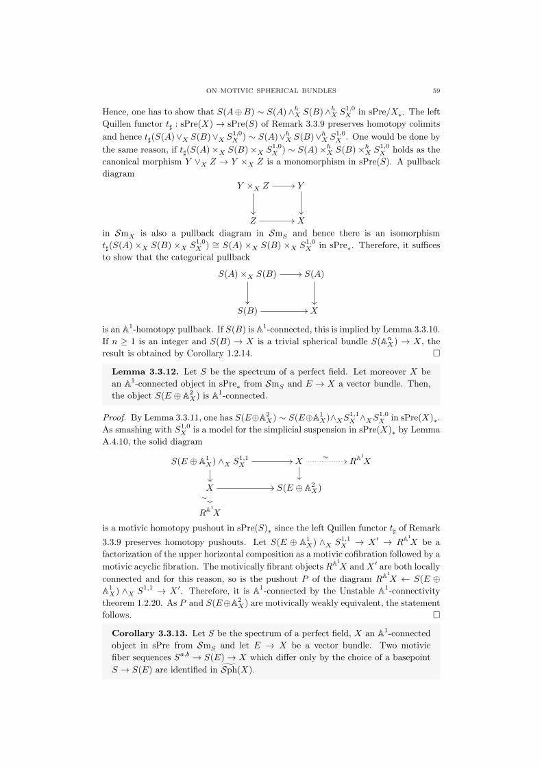
ON MOTIVIC SPHERICAL BUNDLES 59
Hence, one has to show that S(A⊕B) ∼ S(A)∧hX S(B)∧hX S1,0X in sPre/X∗. The left
Quillen functor t] : sPre(X)→ sPre(S) of Remark 3.3.9 preserves homotopy colimits
and hence t](S(A)∨X S(B)∨X S1,0X ) ∼ S(A)∨hX S(B)∨hX S
1,0X . One would be done by
the same reason, if t](S(A)×X S(B)×X S1,0X ) ∼ S(A)×hX S(B)×hX S1,0
X holds as the
canonical morphism Y ∨X Z → Y ×X Z is a monomorphism in sPre(S). A pullback
diagram
Y ×X Z //
Y
Z // X
in SmX is also a pullback diagram in SmS and hence there is an isomorphism
t](S(A) ×X S(B) ×X S1,0X ) ∼= S(A) ×X S(B) ×X S1,0
X in sPre∗. Therefore, it suffices
to show that the categorical pullback
S(A)×X S(B) //
S(A)
S(B) // X
is an A1-homotopy pullback. If S(B) is A1-connected, this is implied by Lemma 3.3.10.
If n ≥ 1 is an integer and S(B) → X is a trivial spherical bundle S(AnX) → X, the
result is obtained by Corollary 1.2.14.
Lemma 3.3.12. Let S be the spectrum of a perfect field. Let moreover X be
an A1-connected object in sPre∗ from SmS and E → X a vector bundle. Then,
the object S(E ⊕ A2X) is A1-connected.
Proof. By Lemma 3.3.11, one has S(E⊕A2X) ∼ S(E⊕A1
X)∧XS1,1X ∧XS
1,0X in sPre(X)∗.
As smashing with S1,0X is a model for the simplicial suspension in sPre(X)∗ by Lemma
A.4.10, the solid diagram
S(E ⊕ A1X) ∧X S1,1
X//
X
∼ // RA1
X
X //
∼
S(E ⊕ A2X)
RA1
X
is a motivic homotopy pushout in sPre(S)∗ since the left Quillen functor t] of Remark
3.3.9 preserves homotopy pushouts. Let S(E ⊕ A1X) ∧X S1,1
X → X ′ → RA1
X be a
factorization of the upper horizontal composition as a motivic cofibration followed by a
motivic acyclic fibration. The motivically fibrant objects RA1
X and X ′ are both locally
connected and for this reason, so is the pushout P of the diagram RA1
X ← S(E ⊕A1X) ∧X S1,1 → X ′. Therefore, it is A1-connected by the Unstable A1-connectivity
theorem 1.2.20. As P and S(E⊕A2X) are motivically weakly equivalent, the statement
follows.
Corollary 3.3.13. Let S be the spectrum of a perfect field, X an A1-connected
object in sPre from SmS and let E → X be a vector bundle. Two motivic
fiber sequences Sa,b → S(E)→ X which differ only by the choice of a basepoint
S → S(E) are identified in Sph(X).
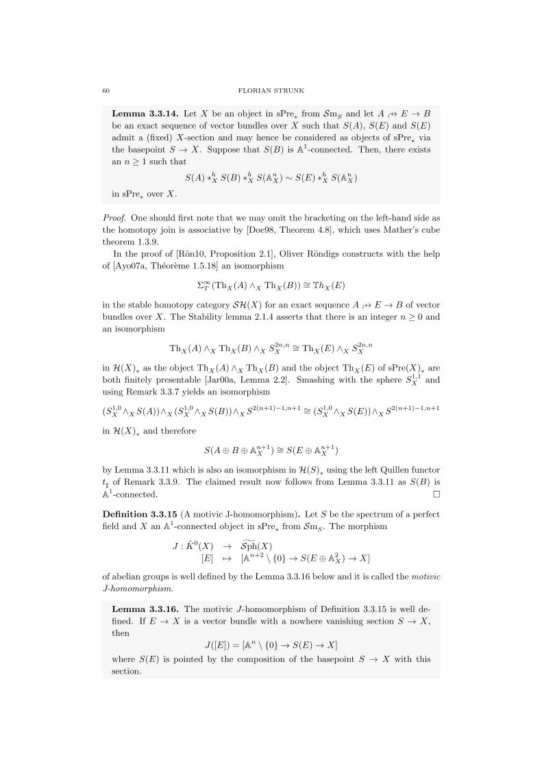
60 FLORIAN STRUNK
Lemma 3.3.14. Let X be an object in sPre∗ from SmS and let A →[ E → B
be an exact sequence of vector bundles over X such that S(A), S(E) and S(E)
admit a (fixed) X-section and may hence be considered as objects of sPre∗ via
the basepoint S → X. Suppose that S(B) is A1-connected. Then, there exists
an n ≥ 1 such that
S(A) ∗hX S(B) ∗hX S(AnX) ∼ S(E) ∗hX S(AnX)
in sPre∗ over X.
Proof. One should first note that we may omit the bracketing on the left-hand side as
the homotopy join is associative by [Doe98, Theorem 4.8], which uses Mather’s cube
theorem 1.3.9.
In the proof of [Ron10, Proposition 2.1], Oliver Rondigs constructs with the help
of [Ayo07a, Theoreme 1.5.18] an isomorphism
Σ∞T (ThX(A) ∧X ThX(B)) ∼= ThX(E)
in the stable homotopy category SH(X) for an exact sequence A →[ E → B of vector
bundles over X. The Stability lemma 2.1.4 asserts that there is an integer n ≥ 0 and
an isomorphism
ThX(A) ∧X ThX(B) ∧X S2n,nX
∼= ThX(E) ∧X S2n,nX
in H(X)∗ as the object ThX(A) ∧X ThX(B) and the object ThX(E) of sPre(X)∗ are
both finitely presentable [Jar00a, Lemma 2.2]. Smashing with the sphere S1,1X and
using Remark 3.3.7 yields an isomorphism
(S1,0X ∧X S(A))∧X (S1,0
X ∧X S(B))∧X S2(n+1)−1,n+1 ∼= (S1,0
X ∧X S(E))∧X S2(n+1)−1,n+1
in H(X)∗ and therefore
S(A⊕B ⊕ An+1X ) ∼= S(E ⊕ An+1
X )
by Lemma 3.3.11 which is also an isomorphism in H(S)∗ using the left Quillen functor
t] of Remark 3.3.9. The claimed result now follows from Lemma 3.3.11 as S(B) is
A1-connected.
Definition 3.3.15 (A motivic J-homomorphism). Let S be the spectrum of a perfect
field and X an A1-connected object in sPre∗ from SmS . The morphism
J : K0(X) → Sph(X)
[E] 7→ [An+2 \ 0 → S(E ⊕ A2X)→ X]
of abelian groups is well defined by the Lemma 3.3.16 below and it is called the motivic
J-homomorphism.
Lemma 3.3.16. The motivic J-homomorphism of Definition 3.3.15 is well de-
fined. If E → X is a vector bundle with a nowhere vanishing section S → X,
then
J([E]) = [An \ 0 → S(E)→ X]
where S(E) is pointed by the composition of the basepoint S → X with this
section.

ON MOTIVIC SPHERICAL BUNDLES 61
Proof. The map
ϕ : Vb(X)→ Sph(X)
defined by ϕ(E) = S(E ⊕ A2X) factorizes through K(X) if ϕ(E) = ϕ(A) ∗hX ϕ(B) for
every exact sequence A →[ E → B and ϕ(AnX) = 0 for n ≥ 0. The map ϕ sends trivial
vector bundles AnX to zero. Let A →[ E → B be an exact sequence of vector bundles
over X. Then, also A⊕A2 →[ E⊕A4 → B⊕A2 is an exact sequence of vector bundles
over X. The object S(B⊕A2) of sPre∗ is A1-connected by Lemma 3.3.12. Therefore,
Lemma 3.3.14 implies that ϕ(E) = ϕ(A) ∗hX ϕ(B) and the motivic J-homomorphism
is well defined. The second claim of the lemma follows from Corollary 3.3.13.
Remark 3.3.17. There are other ways to define a motivic J-homomorphism which
we do not want to consider in this text. For example, an element of GLn may be
considered as an isomorphism An → An mapping An \ 0 to itself. Therefore, one
gets a morphism GLn → hom(An/An \ 0,An/An \ 0) and by composing with a
fibrant replacement functor in the last entry a morphism ψn : GLn → Ω2n,nS2n,n.
After stabilizing, the domain of this morphism may be related to K-Theory. As in
topology, one could hope to get information about motivic homotopy groups of the
spheres by investigating the motivic J-homomorphism.
4. Vanishing results for the J-homomorphism
4.1. A relation with Thom classes
Definition 4.1.1. Let X be an object of sPre∗ from SmS and E → X a vector
bundle over X. A fiber inclusion into the Thom space of E is given as a morphism
inc : An/An \ 0 → E/S(E) = ThS(E) in sPre∗ defined by the diagram
S(An) //
yy
AnX
uuS(E)
//
E
∗yy
// An/An \ 0incuu
∗ // ThS(E)
of simplicial presheaves.
A Thom class for E → X is a morphism u : ThS(E) → Σ∞T (An/An \ 0) in the
stable homotopy category SH(S) such that the composition
Σ∞T (An/An \ 0) Σ∞T (inc)−−−−−→ ThS(E)u−→ Σ∞T (An/An \ 0)
is an isomorphism in SH(S) for some fiber inclusion inc.
Remark 4.1.2. Let Fi−→ E
p−→ X be a smooth fiber bundle in sPre, where X, E
and F are objects from SmS . Consider E∗ as an object of sPre(X)∗. The morphism
b∗(E∗) → t] (E∗) in sPre∗ discussed in Remark 3.3.9, is i∗ : F∗ → E∗, where in
the latter expression F∗ and E∗ are considered as objects of sPre∗. The morphism
b∗(E) → t](E) in sPre is the fiber inclusion i : F → E. It is a little confusing, that
for a pointed X, one may view t] as a functor sPre(X)∗ → sPre∗ as well but t] is
different from t] . There is a natural factorization b∗(E)→ t](E)→ t] (E) in this case
as shown on representants.

62 FLORIAN STRUNK
Lemma 4.1.3. Let X be an object of sPre∗ from SmS , A an object from sPre∗and let E → X be a morphism of sPre∗ such that there exists a section X → E.
Then, there is an isomorphism
E ∧X (A×X)/X∼= E/X ∧A
in sPre∗ which is natural in A and all the appearing operations are models for
their homotopical analogues (confer Definition 1.3.13).
Proof. The pushout diagram
E ∨X (A×X) //
E ×X (A×X)
X // E ∧X (A×X)
shows that the cofibers of the two horizontal maps are isomorphic in sPre∗ and the
diagram
X //
ww
∗ww
E ∨X (A×X)
// E ∨X (A×X)/X
X //
ww
∗ww
E ×X (A×X)
//
E ×X (A×X)/X
∗ww
// ∗ww
E ∧X (A×X)/X
∼= // E ∧X (A×X)/X
where all the horizontal squares are pushouts and where all the vertical edges are
cofiber sequences shows, that E ∧X (A×X)/X is the quotient in sPre∗ of E/X ×A
by E ∨X (A×X)/X but the latter may be identified with E/X ∨A by the diagram
X X
X
X
X //
~~
E
ww
A×X
//
E ∨X (A×X)
∗
// E/X
xx
A // E/X ∨A
in sPre∗. The statement about the homotopical operations is obtained as in the proof
of Lemma 3.3.11 since the projection A×X → X is A1-sharp by Corollary 1.2.14. As
the morphism X → E is assumed to be a section, it is a monomorphism and hence
an A1-injective cofibration, guaranteeing that the wedge sum models its homotopical
analogue.

ON MOTIVIC SPHERICAL BUNDLES 63
Lemma 4.1.4. Let X be an object in sPre∗ from SmS which is connected, let
a ≥ 1 be an integer and let E → X be a vector bundle over X of rank n with a
nowhere vanishing section S → X. Set a = n+ b. Then, there are commutative
diagrams
Ab \ 0 inc //
∼
S(E ⊕ AaX)
qX
(An/An \ 0) ∧ (Aa \ 0) inc∧id // ThS(E) ∧ (Aa \ 0)
and
Ab/Ab \ 0 inc //
∼
ThS(E ⊕ AaX)
∼
(An/An \ 0) ∧ (Aa/Aa \ 0) inc∧id // ThS(E) ∧ (Aa/Aa \ 0)
in sPre∗.
Proof. The diagram of Lemma 3.3.11 may be enlarged to the right to obtain the two
categorical pushout diagrams
S(E) ∧X (AaX \ 0) //
S(E) ∧X AaX
∼ // X
a
E ∧X (AaX \ 0) // S(E ⊕ AaX)/E ∨X AaX
∼ // ThX(E) ∧X (AaX \ 0)
in sPre∗. The monomorphisms in sPre/X are the monomorphisms in sPre over X and
since sPre/X is cartesian closed, the functor − ∧X (AaX \ 0) preserves monomor-
phisms. As S(E) → E is a monomorphism and a pushout of a monomorphism
is a monomorphism (confer Remark 3.1.6), the two diagrams above are homotopy
pushout diagrams. The categorical cofiber of the morphism a may be identified
as ThS(E) ∧ (Aa \ 0) by the previous Lemma 4.1.3. Let qX be the composition
S(E ⊕ AaX) → ThS(E) ∧ (Aa \ 0) of the constructed morphisms in sPre∗. By the
stability of colimits under basechange (confer Remark 1.3.1), the categorical pullback
along the basepoint S → X before collapsing X yields the first commutative diagram
of the statement. Equally, one could use Remark 4.1.2.
For the second assertion, a construction analogous to the above provides a commu-
tative diagram
Ab inc //
∼
E ⊕ AaX
q′X
(An/An \ 0) ∧ Aa inc∧id // ThS(E) ∧ Aa
in sPre∗.

64 FLORIAN STRUNK
The solid diagram
X
X
// ∗
S(E ⊕ AaX) //
E ⊕ AaX
// ThS(E ⊕ AaX)
∼
ThS(E) ∧ (Aa \ 0) // ThS(E) ∧ Aa // ThS(E) ∧ (Aa/Aa \ 0)
consists of homotopy cofiber sequences. Let the pointed morphisms be the categor-
ically induced ones. Then, [Doe98, Lemma 1.4] states that also the right vertical
morphisms constitute a homotopy cofiber sequence, or in other words, there is a weak
equivalence ThS(E⊕AaX)∼−→ ThS(E)∧(Aa/Aa\0) in sPre∗. By the same argument
as above, the second commutative diagram of the statement is obtained.
Proposition 4.1.5. Let X be a A1-connected object in sPre∗ from SmS and let
E → X be a vector bundle over X. Then J(E) = 0 if and only if there exists a
Thom class for E.
Proof. Choose for example the motivic model for the motivic homotopical category.
Suppose first that J(E) = 0. We may assume that E has a nowhere vanishing section,
because otherwise we could choose E ⊕A1. Hence, there exist integers a, b (where we
may assume a, b ≥ 2) and an isomorphism in H∗ making the diagram
An \ 0 ∗h Aa \ 0
∼=
inc∗hinc // S(E) ∗hX S(AaX)
∼=
++ X
Ab \ 0 inc // S(AbX)
33
of fiber sequences commutative. The upper fiber sequence is equivalent to the fiber
sequence Ab \ 0 inc−−→ S(E ⊕AaX)→ X by Lemma 3.3.11 and Lemma A.6.7. As X is
A1-connected, there is a morphism g in H∗ such that the composition
Ab \ 0 inc−−→ S(E ⊕ AaX)g−→ Ab \ 0
is an isomorphism in H∗ by Proposition 1.2.24. The commutative diagram
Ab \ 0 ∧ S1,0
OO
∼=
inc∧S1,0
// S(E ⊕ AaX) ∧ S1,0
OO
∼=
g∧LS1,0
// Ab \ 0 ∧ S1,0
Ab/Ab \ 0 inc // (E ⊕ AaX)/S(E ⊕ AaX)
g′
55
in the homotopy category H∗ where g′ is defined as indicated, shows that the compo-
sition
Ab/Ab \ 0 inc−−→ ThS(E ⊕ AaX)g′−→ Ab/Ab \ 0
is an isomorphism in H∗. Lemma 4.1.4 implies that the composition
(An/An \ 0) ∧ S2a,a inc∧id−−−−→ ThS(E) ∧ S2a,a g′−→ (An/An \ 0) ∧ S2a,a
is an isomorphism in H∗ and the result follows considering Σ∞T .

ON MOTIVIC SPHERICAL BUNDLES 65
For the other direction, let
Σ∞T (An/An \ 0) Σ∞T (inc)−−−−−→ ThS(E)u−→ Σ∞T (An/An \ 0)
be an isomorphism in SH(S). Since all the objects involved are finitely presentable by
[Jar00a, Lemma 2.2], the Stability lemma 2.1.4 asserts that there is an integer c ≥ 0
and an isomorphism
(An/An \ 0) ∧ S2c,c inc∧id−−−−→ ThS(E) ∧ S2c,c g′′−→ (An/An \ 0) ∧ S2c,c
in H∗. Smashing with S1,1 yields an isomorphism
(An/An \ 0)∧ (Aa \ 0) inc∧id−−−−→ ThS(E)∧ (Aa \ 0) g′−→ (An/An \ 0)∧ (Aa \ 0)
where a = c+ 1 and by Lemma 4.1.4, there is an isomorphism
Ab \ 0 inc−−→ S(E ⊕ AaX)g−→ Ab \ 0
in H∗. As X is A1-connected by the same Proposition 1.2.24, the fiber sequence
Ab \ 0 → S(E ⊕ AaX)→ X
is trivial, but as observed in the proof of the other direction, this fiber sequence is by
Lemma 3.3.11 equivalent to the fiber sequence
An \ 0 ∗h Aa \ 0 → S(E) ∗hX S(AaX)→ X
finishing the proof.
4.2. Motivic Atiyah duality and the transfer
Remark 4.2.1. In Remark 2.1.3 we noted, that the category SpΣT (S) of motivic sym-
metric T -spectra can be given the monoidal stable motivic model structure which will
serve as a model for the stable motivic homotopy category SH(S) in the following. In
order to keep the notation clean, we omit the symbol T from the index everywhere.
Due to the closed symmetric monoidal structure, we have in particular an internal
hom-functor hom(−,−) taking values in SpΣ (confer Definition A.2.1). Let S denote
the symmetric T -sphere spectrum Σ∞(S0). Theorem A.2.7 furnishes the stable mo-
tivic homotopy category with the structure of a closed symmetric monoidal category
with unit S and functors ∧L and homR(−,−).
Definition 4.2.2 ([May01a], [May01b]). Let X be a motivic symmetric T -spectrum.
The object DX = homR(X,S) of SH(S) is called the dual object of X (or just the
dual of X).
The adjoint
εXS : DX ∧L X → S
of the identity morphism homR(X,S)→ homR(X,S) is the evaluation map for X.
The object X is called strongly dualizable (or just dualizable), if the morphism
νXS : DX ∧L X = homR(X,S) ∧L X∼= homR(X,S) ∧L homR(S, X)∧L−−→ homR(X ∧L S,S ∧L X)∼= homR(X,X)
is an isomorphism in SH(S).

66 FLORIAN STRUNK
If X is dualizable, the coevaluation map for X is the morphism
ηXS : S id]−−→ homR(X,X)(νXS )−1
−−−−−→ DX ∧L X ∼= X ∧L DX,
where id] is the adjoint of the identity.
For a suspension spectrum X = Σ∞E∗, the morphism
trfES : SηXS−−→ X ∧L DX ∼= DX ∧L X id∧L∆−−−−→ DX ∧L X ∧L X εXS ∧
Lid−−−−−→ S ∧L X ∼= X
in SH(S) is called the transfer map for E (or just the transfer for E). The composition
χ(E) : StrfES−−−→ X
pinch−−−→ S
is called the Euler characteristic of E.
Remark 4.2.3. We recall some terms and statements from algebraic geometry addi-
tionally to the definitions in Remark 1.0.1. Every base scheme X is noetherian and in
particular quasi-compact [Liu02, Exercise 2.3.14]. Hence, every Zariski-fiber bundle
F → E → X has a finite trivializing Zariski covering. Moreover, a Nisnevich-fiber
bundle has a finite trivializing Nisnevich covering (confer [GLMS+00, Lemma 12.2]).
If the base scheme S is a field, then every object of SmS is regular and a reduced
scheme [Liu02, Theorem 4.2.16, 4.3.36]. Moreover, in this case the (finitely many)
irreducible components of an object of SmS are exactly its connected components.
Remark 4.2.4. If A → B → C is a cofiber sequence in SH(S), then if two of its
objects are dualizable, then so is the third (confer [May01b, Theorem 1.9]). This was
used in the proof of the Theorem [RØ06, Theorem 52] cited below as Theorem 4.2.6
in the following way: A Nisnevich distinguished square
W
q
//j// Y
p
U //i // X
defines a homotopy pushout diagram in the motivic homotopy category. Hence, there
are cofiber sequences Σ∞W∗ → Σ∞U∗ → Σ∞C and Σ∞Y∗ → Σ∞X∗ → Σ∞C with
the same homotopy cofiber Σ∞C. Therefore, if three of the objects Σ∞W∗, Σ∞U∗,
Σ∞X∗ and Σ∞X∗ are dualizable in SH(S), then so is the remaining one.
Suppose that X is an object of sPre∗. Then Σ∞X is dualizable in SH(S) if and only
if Σ∞X∗ is dualizable in SH(S) since there is a cofiber sequence S0 → X+ → X and
all the spheres Sa,b are dualizable as they are invertible (confer [May01a, Definition
2.8]). Moreover, if two objects X and Y from SpΣ are dualizable, then so is X ∧L Y[May01a, Proposition 2.7].
Theorem 4.2.5 ([Hu05, Theorem A.1]). Let S be the spectrum of a field and
let X ∈ SmS be a smooth projective scheme. Then, X∗ is dualizable.
Theorem 4.2.6 ([RØ06, Theorem 52]). Let S be the spectrum of a field of
characteristic zero and let X ∈ SmS be a smooth quasi-projective scheme. Then,
X∗ is dualizable.

ON MOTIVIC SPHERICAL BUNDLES 67
Remark 4.2.7. If S is the spectrum of a field of arbitrary characteristic, it is not
known, whether for an affine scheme X →[ AnS of SmS , the spectrum Σ∞X∗ is du-
alizable in SH(S). With the following argument, one may show the dualizability of
Σ∞X∗ in a concrete situation. Consider the two pullback diagrams
X
_
// // PX_
X∞_
oooo
An // // Pn Pn−1oooo
of schemes, where PX denotes the projective closure of X. Suppose PX is smooth and
hence an object of SmS . There is a homotopy cofiber sequence X∗ PX∗ → PX/Xand Theorem 4.2.5 together with Remark 4.2.4 yield, that the suspension spectrum
of PX∗ is dualizable and therefore the suspension spectrum of X∗ is dualizable, if the
suspension spectrum of PX/X is dualizable. Suppose moreover, that X∞ is smooth
and hence an object of SmS . Then, the Homotopy purity theorem [MV99, Theorem
3.2.23] shows, that the suspension spectrum of PX/(PX \X∞) = PX/X is dualizable
(confer [RØ06, Theorem 52]).
Remark 4.2.8. Let p : E → X be an object of SmX . The Quillen adjunction
p] : sPre(E)∗ → sPre(X)∗ : p∗
of Remark 3.3.9 can be promoted to a Quillen adjunction
p] : SpΣ(E)→ SpΣ(X) : p∗
of motivic symmetric spectra, where we omit the symbol from the notation as only
the pointed setting is considered (confer [Ayo07b, Theoreme 4.5.23] using [Ayo07b,
Lemme 4.3.34] which works for the category SmS of this text). The projection formula
of Remark 3.3.9 and the isomorphism p∗TX∼= TE is used to construct the prolongation
of p] where for details we refer to [Ayo07b, Remarque 4.3.18]. In particular, one has
p]Σ∞ ∼= Σ∞p] and p∗Σ∞ ∼= Σ∞p∗. The functor p∗ is strong symmetric monoidal by
[Hov01b, Theorem 9.3]. By abuse of notation, we will use the same notation for the
derived functors of p] and p∗ respectively.
Theorem 4.2.9 (confer [May95, Proposition III.1.9]). Let p : E → X be a
morphism of objects from SmS . If the object Y of SH(X) is dualizable, then so
is p∗Y and there is an isomorphism
p∗DY ∼= Dp∗Y
in SH(E).
4.3. A motivic version of Brown’s trick
Remark 4.3.1. Let S be the spectrum of a field. In this section, we change our
notation and let SmS be the category of smooth quasi-projective schemes of finite type
over S to be able to use the results from [Ayo07a] and [Ayo07b]. The unpublished
manuscript [Ron05] asserts though, that this restriction is not necessary if we use
[Ron05, Corollary 3.14] instead of [Ayo07a, Corollaire 1.4.4].

68 FLORIAN STRUNK
Lemma 4.3.2. Let F → Yf−→ X be a smooth Nisnevich fiber bundle and
suppose that Σ∞F∗ is dualizable in SH(S). Then, Σ∞Y∗ is dualizable in SH(X)
and the transfer
trfYX : Σ∞X∗ → Σ∞Y∗
in SH(X) is defined.
Proof. Let ui : Ui → X be a finite trivializing Nisnevich covering for the fiber
bundle which exists by Remark 4.2.3. We have to show that the morphism
νYX : homRX(Σ∞Y∗,SX) ∧LX Σ∞Y∗∼= homRX(Σ∞Y∗,SX) ∧LX homRX(SX ,Σ
∞Y∗)
→ homRX(Σ∞Y∗ ∧LX SX ,SX ∧
LX Σ∞Y∗)
∼= homRX(Σ∞Y∗,Σ∞Y∗)
in SH(X) is an isomorphism where we write Y instead of Σ∞Y∗ in the upper index. By
[Ayo07a, Corollaire 1.4.4], it suffices to show that u∗i (νYX) is an isomorphism in SH(Ui)
for every i. The functor u∗i is strong symmetric monoidal by Remark 4.2.8 and since
ui is smooth, there is a natural isomorphism u∗i (homRX(E,D)) ∼= homRUi(u∗iE, u
∗iD)
by [Ayo07a, Proposition 2.3.54]. Therefore, it suffices to show, that νu∗iΣ∞Y∗Ui
is an
isomorphism, or in other words, that u∗iΣ∞Y∗
∼= Σ∞u∗i Y∗ is dualizable in SH(Ui).
Since the bundle is trivial on the Ui, one has u∗i (Y∗)∼= (Ui × F )∗ in sPre(Ui)∗.
Considering the composite morphism Ui → X → S defined by t ui, the assertion
follows from Theorem 4.2.9, as Σ∞F∗ is dualizable in SH(S) by assumption.
Corollary 4.3.3. Let F → Yf−→ X be a smooth Nisnevich fiber bundle and
suppose that Σ∞F∗ is dualizable in SH(S). Let p : E → X be a vector bundle
and q : D → Y the pullback bundle along f . Then, Σ∞S(D)∗ is dualizable in
SH(S(E)) and the transfer
trfS(D)S(E) : Σ∞S(E)∗ → Σ∞S(D)∗
in SH(S(E)) is defined.
Proof. The Nisnevich fiber bundle F × (An \ 0) → S(D) → S(E) obtained by
pullback along S(E)→ X is smooth and Σ∞F∗∧Σ∞(An\0)∗ is dualizable in SH(S)
by Remark 4.2.4. Hence, the the Lemma 4.3.2 shows that Σ∞S(D)∗ is dualizable in
SH(S(E)).
Remark 4.3.4. Consider the setting of Corollary 4.3.3. There is a commutative
diagram
p]p∗Σ∞Y∗
εΣ∞Y∗
oop]p∗ trfYX
p]p∗Σ∞X∗
εΣ∞X∗
Σ∞Y∗ ootrfYX
Σ∞X∗
in SH(X) where ε is the unit of the adjunction (p], p∗) of Remark 4.2.8.

ON MOTIVIC SPHERICAL BUNDLES 69
Hence, by the compatibility of the transfer with p∗ (confer Theorem 4.2.9), there is a
commutative diagram
p]Σ∞S(D)∗
ε′Σ∞Y∗
oop] trf
S(D)
S(E)
p]Σ∞S(E)∗
ε′Σ∞X∗
Σ∞Y∗oo
trfYXΣ∞X∗
in SH(X). Applying the functor t] : SH(X)→ SH(S) and omitting some decoration
by abuse of notation, one has a commutative diagram
Σ∞S(D)∗
Σ∞q∗
oo trfΣ∞S(E)∗
Σ∞p∗
Σ∞Y∗ ootrf
Σ∞X∗
in SH(S). Hence, by taking the homotopy cofibers of the vertical morphisms and
considering the natural transformation of the fiber inclusion of Remark 3.3.9, there is
a commutative diagram
Σ∞F∗ ∧ Σ∞S2n,n
r
ww
oo trf′
Σ∞S2n,n
incww
ThS(D) ootrf′ ThS(E)
in SH(S), where the upper morphism trf ′ is a suspension of trfFS in SH(S).
Theorem 4.3.5. Let S be the spectrum of a perfect field and F an A1-connected
object from SmS such that Σ∞F∗ is dualizable in SH(S) with invertible Euler
characteristic χ(F ). Let moreover F → Y → X be a smooth Nisnevich fiber
bundle and E → X a vector bundle with pullback bundle D → Y along Y → X.
Suppose that X is A1-connected. Then, J(D) = 0 implies J(E) = 0.
Proof. Since the whole proof takes place in the stable motivic homotopy category
SH(S), we omit writing the strong monoidal suspension spectrum functor Σ∞ ev-
erywhere. Let J(D) = 0. By Proposition 4.1.5, there hence exists a Thom class
w : ThS(D)→ S2n,n for the vector bundle D → Y . We have to show that there exists
a Thom class u : ThS(E)→ S2n,n for E → X since this implies J(E) = 0 by the same
Proposition 4.1.5.

70 FLORIAN STRUNK
Consider the diagram
(An \ 0)∗vv
F∗ ∧ (An \ 0)∗ ootrf
ww
(An \ 0)∗
xx
S(D)∗
q∗
oo trf
S(E)∗
p∗
S0,0
a∗
vvF∗oo trf
j∗
ww
S0,0
b∗xxY∗
oo trf
X∗
S2n,n
a∗∧S2n,n
vv
F∗ ∧ S2n,n oo trf ∧S2n,n
r
ww
S2n,n
incyy
ThS(D) ootrf′
w
ThS(E)
u
ssS2n,n
and define u as the indicated composition w trf ′. We have to show that
S2n,n inc−−→ ThS(E)u−→ S2n,n
is an isomorphism in SH(S) and by a Yoneda argument it suffices to show that this
composition induces an isomorphism on 〈S2n,n,−〉SH(S). In the remaining part of the
proof, we will omit writing the SH(S) in the index of the homotopy classes. By the
commutativity of the diagram above it is the same to show, that the composition
w r (trf ∧S2n,n) induces an isomorphism on 〈S2n,n,−〉. The condition on the Eu-
ler characteristic of F is, that the composition pinch trf induces an isomorphism on
〈S0,0,−〉. The composition pinch a∗ is the identity on S0,0 and therefore an isomor-
phism on the homotopy classes 〈S0,0,−〉. Remark 2.2.4 and Proposition 2.2.5 yield,
that a∗ induces an isomorphism on 〈S0,0,−〉 and therefore pinch is an isomorphism on
these homotopy classes as well. This implies that trf : S0,0 → F∗ is an isomorphism
on 〈S0,0,−〉. It suffices therefore by the invertibility of the suspension with S2n,n to
show, that w r is an isomorphism on 〈S2n,n,−〉. The composition r (a∗ ∧ S2n,n)
is the fiber inclusion S2n,n → ThS(D) and by assumption, w r (a∗ ∧ S2n,n) in-
duces an isomorphism on 〈S2n,n,−〉. It was already observed that (a∗∧S2n,n) induces
an isomorphism on these homotopy classes and hence it is implied that w r is an
isomorphism on 〈S2n,n,−〉, showing the result.

ON MOTIVIC SPHERICAL BUNDLES 71
4.4. Dualizability of GLn/NT
Theorem 4.4.1 (Ayoub, Rondigs [Ron10, Lemma 4.2]). Let S be the spectrum
of a field and X a projective curve from SmS . For any line bundle E → X, one
has ThX(E ⊗ E) ∼ S2,1X in SH(X).
Corollary 4.4.2. Let S be the spectrum of a perfect field and X a projective
curve from SmS which is A1-connected. For any line bundle E → X, one has
J(E ⊗ E) = 0.
Proof. This can be done as in the proof of Lemma 3.3.14 by considering the vector
bundle (E⊗E)⊕A1X → X whose associated spherical bundle admits an X-section.
Remark 4.4.3. There are exactly one example of a projective curve from SmS which
is A1-connected and this is P1 [AM11, Proposition 2.1.12].
Remark 4.4.4. Let S be the spectrum of a field k. The algebraic group NTn of mono-
mial matrices introduced in Definition 3.2.4, acts freely from the right as a subgroup
on GLn. Set A = OGLn(GLn), B = ONT (NT ) and consider the k-algebra
AB = a ∈ A | ∆(a) = a⊗ 1
of invariants. The groupNT is reductive, id est the radical of the connected component
of the unit is isomorphic to a product of Gm. By the former Mumford conjecture which
is now Haboush’s theorem [Hab75, Theorem 5.2], it is geometrically reductive and
therefore satisfies the assumption of Nagata’s theorem [Dol94, Theorem 3.3] stating
that AB is finitely generated as a k-algebra (confer also [MFK94, Theorem A.1.0]).
Define GLn/NT as the spectrum of the k-algebra AB . It is shown in [MFK94,
Theorem 1.1] that p : GLn → GLn/NT induced by the inclusion on k-algebras is
a categorical quotient. By [Bor91, Theorem 6.8], there exists a geometric quotient
for the canonical action of NT on GLn. As a geometric quotient is in particular
a categorical quotient (confer [Bor91, 6.16] or [MFK94, Proposition 0.1]), the two
schemes coincide. In particular, by [Bor91, Theorem 6.8], the scheme GLn/NT is
smooth and quasi-projective and hence by the above observations an element of SmS .
This geometric quotient GLn/NT is also the fppf-quotient in the category of fppf-
sheaves (confer Section 3.1) since [Jan87, 5.6.8] states, that the fppf-quotient is a
scheme. Therefore, Lemma 3.1.14 together with Remark 3.1.6 imply, that the mor-
phism p : GLn → GLn/NT is fppf-locally trivial.
As smoothness of a morphism may be checked fppf-locally by [Gro67, Proposi-
tion 17.7.4], the morphism p is smooth and hence also etale-locally trivial as it has
sections etale-locally [Gro67, Corollaire 17.16.3]. The author does not know, if the
morphism p is Nisnevich-locally trivial and therefore, if GLn/NT is the Nisnevich-
quotient GLn//N isNT .
Lemma 4.4.5. Let S be the spectrum of an algebraically closed field k. Then,
[S,GLn/NT ]A1∼= ∗.
Proof. We know already, that the quotient morphism p : GLn → GLn/NT is etale-
locally trivial. Let a : S → GLn/NT be a k-rational point. As k is algebraically
closed, the a may be lifted along some trivializing etale morphism ui : Ui → GLn/NT
for p.

72 FLORIAN STRUNK
Together with the canonical section Ui → Ui ×NT , one obtains a lift b : S → GLn of
a along p, which corresponds to an invertible matrix M with entries in k. This matrix
may be written as a finite product M = E1 . . . EkD, where
Ei =
1
1 λmini. . .
1
1
and D =
1
1. . .
1
d
with d 6= 0 by [Lan02, Proposition 9.1]. Let d : S → GLn be the k-rational point
corresponding to the matrix D. One may construct an evident homotopy A1 → GLnfromD to the k-rational point dk : S → GLn/NT corresponding to EkD and therefore,
the morphisms d and dk are equal in the (unpointed) motivic homotopy category as A1
induces a cylinder object for the A1-local injective structure (confer Remark 1.1.20).
After a finite iteration of this method, it is shown that the morphisms b and d are
equal in the motivic homotopy category and, for the same reason, that the morphisms
a = pb and pd : S → GLn/NT are equal in the motivic homotopy category. Since D
is a monomial matrix, the morphism pd : S → GLn/NT is the same as the morphism
pe : S → GLn/NT where e : S → GLn corresponds to the identity matrix. This
shows the result.
Lemma 4.4.6. Let S be the spectrum of a field of characteristic zero. Then, the
spectrum Σ∞GLn/NT∗ is dualizable in SH(S).
Proof. Remark 4.4.4 shows that GLn/NT is a quasi-projective scheme in SmS and
hence the result follows from Theorem 4.2.6.
Remark 4.4.7. Now, a strategy for proving vanishing results for the J-homomorphism
could be the following: Let S be the spectrum of a perfect field k, let X ∈ SmS be an
A1-connected scheme and E → X a vector bundle of rank n.
Find an algebraic subgroup H of GLn such that:
(1a) The Zariski-quotient G//ZarH is an object of SmS or
(1b) the Nisnevich-quotients G//N isH and E//
N isH are objects from SmS .
Lemma 3.1.19 and Lemma 3.1.20 provide a vector bundle D → Y , where Y = E//N isH
and a smooth Nisnevich-fiber bundle
D //
q
E
p
F // Yf// X
where F = G//N isH.
(2) Show that [S, F ]A1 is trivial.
Moreover,
(3a) show that F is projective or
(3b) show that F is quasi-projective and the characteristic of k is zero or
(3c) show that F is affine and the method of Remark 4.2.7 applies.
In all of these cases (3 -), it is implied that Σ∞F∗ is dualizable in SH(S) by Theorem
4.2.5 or Theorem 4.2.6.

ON MOTIVIC SPHERICAL BUNDLES 73
(4) Show that the Euler characteristic χ(F ) is invertible.
If conditions (1)-(4) hold, Theorem 4.3.5 states, that J(D) = 0 implies J(E) = 0. The
question of deciding whether J(D) = 0 can be considered as easier, since the vector
bundle D admits a reduction of the structure group to H.
Therefore, it would be nice to find a large subgroup H of GLn, fulfilling the prop-
erties. A naive solution would be H = GL1 × GLn−1 since one may then split of a
line bundle successively and has to show the vanishing of J only for line bundles as
in Corollary 4.4.2. Unfortunately, the Euler characteristic of the quotient G//N isH does
not seem to be invertible since the Euler characteristic of the topological quotients
O(2n)/(O(2)×O(2n− 2)) and U(n)/(U(1)× U(n− 1)) is n.
The manuscript [Ebe] proposes H = NT , where NT denotes the normalizer of the
standard maximal torus. The connected topological space O(2n)/NT has in fact Euler
characteristic one (confer [Ebe, Theorem 5.4]) and the observations in the reference
can be applied to the complex case U(n)/NT as well. Hence, NT could be a good
candidate for a motivic reduction process as described above.
74 FLORIAN STRUNK
A. Appendix
This section contains preliminaries on model categories which are used throughout
the whole text. Particularly monoidal structures on model categories are introduced
and pointed model categories with their suspension and loop functors are described.
Afterwards we focus on fiber and cofiber sequences in pointed model categories.
A.1. Preliminaries on model categories
Definition A.1.1 ([Hov99, Section 1.1]). Let C be a category. A functorial factor-
ization (α, β) in C is a pair of endofunctors on the morphism category of C such that
for every morphism f of C there is a factorization f = β(f) α(f).
Let i : A → B and p : X → Y be morphisms in C. One says that i fulfills the left
lifting property (LLP) with respect to p and p fulfills the right lifting property (RLP)
with respect to i if for every commutative solid diagram
A //
i
X
p
B //
l
>>
Y
a dotted arrow l exists such that everything commutes. In this case, l is called a lift
of the diagram.
Definition A.1.2 ([Hov99, Definition 1.1.3]). Let C be a category. A model structure
on C consists of three subcategories we, cof, fib of C and two functorial factorizations
(α, β), (γ, δ) in C such that the following properties are fulfilled:
(Two out of three) Let f and g be two composable morphisms in C. If two of
the morphisms f , g or gf are in we, then so is the third.
(Retracts) Let f and g be morphisms in C and f a retract of g in the morphism
category of C. If g is in we, cof or fib, then so f lies in the same subcategory.
(Liftings) The morphisms in we∩ cof have the LLP with respect to the morphisms
in fib and the morphisms in we ∩ fib have the RLP with respect to the morphisms
in cof.
(Factorizations) Let f be a morphisms in C then
α(f) ∈ cof and β(f) ∈ we ∩ fib,
γ(f) ∈ we ∩ cof and δ(f) ∈ fib.
The morphisms in we are called weak equivalences and they are denoted by an arrow of
the type∼−→ in the sequel. Morphisms in cof are denoted by and called cofibrations.
The morphisms in fib are denoted by and called fibrations. A cofibration in we
is called an acyclic cofibration and a fibration in we is called an acyclic fibration. A
bicomplete category is a category having all limits and colimits of diagrams indexed by
a small category. A pair consisting of a bicomplete category C and a model structure
on C is called a model category.
Definition A.1.3 ([Hir03, Definition 8.1.15]). An object X of a model category C is
called cofibrant if the map ∅ → X from the initial object to X is a cofibration. Dually,
X is called fibrant if the map X → ∗ from X into the terminal object is a fibration.
A cofibrant replacement functor consists of a functor Q : C → C such that every QX
is cofibrant and a natural weak equivalences QX → X. Dually, a fibrant replacement

ON MOTIVIC SPHERICAL BUNDLES 75
functor consists of a functor R : C → C such that every RX is fibrant and a natural
weak equivalences X → RX.
Definition A.1.4 ([Hov99, Definition 1.2.4]). A cylinder object for an object X of a
model category C is an object X∧I of C together with a cofibration iX : XtX → X∧Iand a weak equivalence pX : X ∧ I → X such that their composition is a factorization
of the fold map X tX → X.
Two morphisms f, g : X → Y in C are called (left) homotopic if there is a map
H : X ∧ I → Y for some cylinder object X ∧ I of X such that the diagram
X
i0 ##
f
**X tX //iX // X ∧ I H // Y
Xg
44
i1
;;
commutes. In this case one writes f ∼ g.
A morphism f is called a homotopy equivalence if there exists a morphisms g such
that fg ∼ id and gf ∼ id.
Remark A.1.5. Since the existence of functorial factorizations is part of our definition
of a model structure, there exists both a cofibrant and a fibrant replacement functor
and a functorial cylinder object in any model category. The left homotopy relation
is not an equivalence relation in general but this is the case if X is cofibrant and Y
is fibrant and one may then define the set hom(X,Y )/∼. Moreover, in this case it
does not matter which cylinder object is used to determine whether two maps are
homotopic (confer [Hov99, Proposition 1.2.5]).
Theorem A.1.6 (Quillen, [Hir03, Theorem 8.3.5, 8.3.10], [Hov99, Theorem
1.2.10]). Let C be a model category. Then the homotopy category HoC of C exists.
It has, fixing the cofibrant Q and the fibrant replacement functor R induced by
the functorial factorization, the same objects as C and morphisms
homHoC(X,Y ) = homC(RQX,RQY )/∼denoted by [X,Y ] with composition [g] [f ] = [g f ] and identities [id]. The
canonical full functor [−] : C → HoC sends a map to an isomorphism if and only
if the map is a weak equivalence. In particular, if f ∼ g then [f ] = [g] which
holds even if f and g do not have a cofibrant domain and fibrant codomain. If X ′
is cofibrant and weakly equivalent to X and if Y ′ is fibrant and weakly equivalent
to Y , then there is an isomorphism homC(RQX,RQY )/∼ ∼= homC(X′, Y ′)/∼.
Remark A.1.7. For a pair (C,we) consisting of a category C together with a sub-
category we, one is interested in forming a category C[we−1] inverting the morphisms
in we. The previous Theorem A.1.6 guarantees the existence of such a category for
a pair (C,we) obtained from a model category. A more general setting is considered
in [DHKS04] where the authors focus on pairs (C,we) called a homotopical category
if they are fulfilling some axioms [DHKS04, 31.3]. In particular, a model category
defines a homotopical category ignoring its cofibrations and fibrations and therefore
different model structures on the same category and with the same weak equivalences
determine the same homotopical category.

76 FLORIAN STRUNK
Remark A.1.8. The set of maps homHoC(X,Y ) may be interpreted as the set of
equivalence classes of zigzags
X∼←− · → · ∼←− Y
where the equivalence relation is defined by saying that in any commutative diagram
· //
· \\
·
//
OO
yy
·
OO
ee
X · //oo · oo Y
· //
OOee
·
OO
yy
consisting of weak equivalences except for the horizontal maps in the middle column,
the top and the bottom row are equivalent [DHKS04, Proposition 11.2].
Definition A.1.9 ([Hov99, Definition 1.3.1]). An adjunction F : C D : G is called
a Quillen adjunction if the left adjoint F preserves cofibrations and acyclic cofibra-
tions and the right adjoint G preserves fibrations and acyclic fibrations. A Quillen
adjunction defines an adjunction LF : HoC HoD : RG the derived adjunction
where the left derived functor LF is given by FQ(−) (on representants) and the right
derived functor RG is defined by GR(−) (on representants). The adjunction (F,G)
is called a Quillen equivalence if its derived adjunction (LF,RG) is an equivalence of
categories.
Remark A.1.10. It follows from Theorem A.1.6, that one may use any cofibrant re-
placement functor to construct the left derived functor of a left Quillen functor. The
dual statement holds for right derived functors as well. The expression on represen-
tants in context with LF means, that for a morphism in the homotopy category one
first has to choose a representant f in C in order to apply the cofibrant replacement
functor Q : C → C and afterwards F . The theory then guarantees, that FQ(f) is equal
to FQ(f ′) in the homotopy category of D for any other choice f ′ of a representant.
Definition A.1.11 ([AR94]). Let C be a category and let κ be a regular cardinal,
which is an infinite cardinal that cannot be written as a union indexed by a strictly
smaller cardinal of strictly smaller cardinals.
A diagram D : I → C is called κ-directed if I is a κ-directed partially ordered set,
this is a partially ordered set such that every subset of cardinality strictly smaller then
κ has an upper bound. A directed diagram is a κ-directed diagram for some κ.
A κ-directed colimit is a colimit of a κ-directed diagram and a directed colimit is a
colimit of a directed diagram.
An object T of C is called κ-presentable if the functor hom(T,−) : C → Set preserves
κ-directed colimits.
An object T of C is called small if it is κ-presentable for some κ and it is called
finitely presentable if it is |N|-presentable.
A category C is called accessible if it contains a set of κ-presentable objects such
that every object of C is a κ-directed colimit of those objects.
The category C is called locally presentable if it is cocomplete and accessible.
Remark A.1.12. By [AR94, Theorem 1.5], a category has all filtered colimits, if and
only if it has all directed colimits. A functor from C preserves all filtered colimits if and
only if it preserves all directed colimits. A κ-presentable object is always κ′-presentable

ON MOTIVIC SPHERICAL BUNDLES 77
for larger regular cardinals κ′ > κ and hence it is usually a stronger property to be
finitely presentable than just to be small. An object T is finitely presentable if and
only if the functor hom(T,−) commutes with all directed (or equivalently filtered)
colimits.
Definition A.1.13 ([Hov99, Definition 2.1.17]). A model category C is called (I,J )-
cofibrantly generated if for sets of morphisms I = A → B and J = C → D the
following properties are fulfilled:
(Smallness) The A (respectively the C) are small with respect to diagrams consist-
ing only of I-cell complexes (respectively J -cell complexes) where a relative I-cell
complex is a morphism X0 → colimα<λXα from the initial object of a sequential
diagram into its colimit where each step of the diagram is given by a pushout
A //
Xα
B // Xα+1
and colimβ<αXβ = Xα when α is a limit ordinal.
(Cofibrations) Cofibrations are exactly retracts of relative I-cell complexes.
(Acyclic cofibrations) Acyclic cofibrations are exactly retracts of relative J -cell
complexes.
A model category is called combinatorial if it is locally presentable and cofibrantly
generated [Lur09, Definition A.2.6.1].
Definition A.1.14 ([DRØ03a, Definition 3.4]). An (I,J )-cofibrantly generated mo-
del category C is called
• finitely generated if the domains and codomains of I and J are all finitely
presentable,
• weakly finitely generated if the domains and codomains of I are all finitely
presentable, the domains of J are small and there is a set J ′ of generating
acyclic cofibrations with finitely presentable domains and codomains such that
a morphism f : X → Y into a fibrant object is a fibration if and only if f has
the RLP with respect to all maps in J ′.
Remark A.1.15. It is described in [Hov99, Section 7.4], that the usual model struc-
tures on simplicial sets and chain complexes are finitely generated but the usual model
structure on topological spaces is not because one has to restrict to diagrams of cofi-
brations.
Lemma A.1.16 ([DRØ03a, Lemma 3.5]). Let C be a weakly finitely generated
model category. Then the classes of
• weak equivalences,
• acyclic fibrations,
• fibrations with fibrant codomain,
• fibrant objects
are closed under filtered colimits each.

78 FLORIAN STRUNK
Theorem A.1.17 ([Hir03, Theorem 11.6.1], [Lur09, Proposition A.2.8.2]). Let
C be a cofibrantly generated model category and I an essentially small category.
Then there is a cofibrantly generated model structure on the functor category
Fun(I, C) called the projective model structure with weak equivalences and fi-
brations defined objectwise. It is combinatorial, if C is combinatorial. Moreover,
if C is a combinatorial model category, there is a combinatorial model structure
on the functor category Fun(I, C) called the injective model structure with weak
equivalences and cofibrations defined objectwise. The identities
id : Fun(I, C)proj Fun(I, C)inj : id
are a Quillen equivalence.
Definition A.1.18 ([Lur09, Remark A.2.8.8]). Let C be a cofibrantly generated mo-
del category and I a small category, then colim : Fun(I, C)proj C : ∆ is a Quillen
adjunction and the left adjoint of the associated derived adjunction is called the ho-
motopy colimit. If C is combinatorial then ∆ : C Fun(I, C)inj : lim is a Quillen
adjunction and the right adjoint of the associated derived adjunction is called the
homotopy limit.
When the symbol hocolim is used, we mean the specific functor
hocolim : Fun(I, C) → CD 7→ colim(Q(D))
where Q is the cofibrant replacement functor of Fun(I, C)proj obtained from the func-
torial factorization. The functor holim : Fun(I, C)→ C is defined dually.
Remark A.1.19. The homotopy colimit and the homotopy limit are not the colimit
and the limit in the homotopy category. As we discuss below, this is only true for
coproducts and products. Moreover, they do not depend on the homotopy category
only but it suffices to consider the underlying homotopical category of a model category
(confer [DHKS04] or [Shu09, Proposition 4.8]). In particular, all statements concerning
homotopy colimits and homotopy limits in one model category are also valid in a
Quillen equivalent model category as they define the same (saturated) homotopical
category [Shu09, Definition 3.11]. One should note, that the homotopy colimit functor
Lcolim : HoFun(I, C)proj → HoC can only be applied to diagrams in C and not
necessarily to diagrams in HoC.
Definition A.1.20 ([Hir03, Definition 13.1.1]). A model category is called left proper
if every pushout of a weak equivalence along a cofibration is again a weak equivalence,
right proper if every pullback of a weak equivalence along a fibration is again a weak
equivalence and proper if it is left proper and right proper.
Remark A.1.21. To calculate the homotopy colimit of a certain diagram in a model
category, one replaces that diagram cofibrantly in the projective model structure. This
cofibrant replacement is usually not given by just replacing all the arrows and objects
cofibrantly. Nevertheless, this is true for certain diagrams. Particularly, to calculate
a homotopy pushout (or dually a homotopy pullback)
Af
//
g
C
B // hocolim
holim //
C
p
Bq// A

ON MOTIVIC SPHERICAL BUNDLES 79
in a left proper model category C, it suffices to replace f or g with a cofibration (or
dually p or q with a fibration if C is right proper), take the ordinary pushout (or
pullback) in C and consider the resulting diagram in the homotopy category (confer
[Hir03, Corollary 13.3.8]).
If the object B is the terminal object of C, the above homotopy pushout (or homo-
topy pullback) is called the homotopy cofiber of the map f (or the homotopy fiber of the
map p) [Hir03, Definition 13.4.3]. Whenever we speak of the object hocofib(f) in a left
proper model category C (or of the object hofib(f) in a right proper model category C),we mean the categorical pushout of the diagram ∗′′ ← A → B where the cofibration
A ∗′′ is obtained by the functorial factorization of C (or the categorical pullback
of the diagram ∗′ → A← C where the fibration ∗′ → A is obtained by the functorial
factorization of C). In particular, one has an actual diagram A→ B → hocofib(f) in
C (or an actual diagram hofib(f)→ C → A in C).A diagram D : I → C is a homotopy colimit diagram (or homotopy limit diagram) if
the canonical map hocolimD → colimD (or if the canonical map limD → holimD) is
a weak equivalence. The two upper diagrams are diagrams in the homotopy category
HoC only since the dotted arrows need not to be represented by morphisms in C.Left Quillen functors F : C → D preserve homotopy colimits (and dually, right
Quillen functors preserve homotopy limits) as the diagram
Fun(I, C)projcolim //
F∗
C
F
Fun(I,D)projcolim // D
of left Quillen functors commutes and derivation goes along with composition in model
categories [Hov99, Theorem 1.3.7].
Lemma A.1.22 (Glueing/Coglueing, [Hir03, Proposition 13.5.4, 13.3.9]). Con-
sider the commutative cubes
A′ //
X ′
A
∼>>
//
X
∼>>
B′ // P ′
B
∼>>
// P
>>
F ′ // E′
F
>>
//
E
∼>>
B′ // X ′
B
∼>>
// X
∼>>
where the front and the back are pushout squares in the first cube and pullback
squares in the second cube and where the dotted arrows are the induced maps
respectively. If C is left proper, then the induced map of the left cube is a weak
equivalence. If C is right proper, then the induced map of the right cube is a
weak equivalence.

80 FLORIAN STRUNK
A.2. Monoidal model categories
Definition A.2.1 ([Bor94b, Section 6.1]). A symmetric monoidal category (C,∧, I)consists of a category C together with a functor
− ∧− : C × C → C
and an object I ∈ C, natural associativity isomorphisms (X ∧ Y ) ∧Z → X ∧ (Y ∧Z),
natural unit isomorphisms (I ∧ X) → X as well as natural symmetry isomorphisms
X ∧ Y → Y ∧X subject to certain coherence laws.
A closed symmetric monoidal category is a symmetric monoidal category (C,∧, I)together with a functor
hom(−,−) : Cop × C → Cand an adjunction
− ∧X : C C : hom(X,−).
Definition A.2.2 ([Hov99, Definition 4.2.6]). A monoidal model structure on a closed
symmetric monoidal category (C,∧, I) is a model structure on C such that the following
properties are fulfilled:
(Pushout product) Let i : A B and j : C D be cofibrations in C then their
pushout product
ij : (B ∧ C)∐
(A∧C)(A ∧D)→ B ∧D
is a cofibration and an acyclic cofibration if i or j is a weak equivalence.
(Unit) A unit property which is automatically fulfilled for a cofibrant unit I.
Remark A.2.3. For a symmetric monoidal model category and a cofibrant object
X the adjunction (−∧X,hom(X,−)) is a Quillen adjunction [Hov99, Remark 4.2.3].
The usual model structure on the closed symmetric monoidal category (sSet,×,∆0)
of simplicial sets is monoidal [Hov99, Proposition 4.2.8].
Definition A.2.4 ([Bor94b, Section 6.2]). A (lax) monoidal functor F : C → Dbetween symmetric monoidal closed categories (C,∧C , IC) and (D,∧D, ID) consists of
a functor F : C → D, natural morphisms
tF : F (X) ∧D F (Y )→ F (X ∧C Y )
and a morphism eF : ID → F (IC) subject to certain coherence laws. A monoidal
functor is called strong if all its structure maps t and e are isomorphisms.
A monoidal natural transformation η : F → G of two monoidal functors F and G
from C to D is a natural transformation η : F → G such that all the diagrams
F (X) ∧D F (Y )ηX∧ηY
//
tF
G(X) ∧D G(Y )
tG
F (X ∧C Y )ηX∧Y
// G(X ∧C Y )
IDeF
||
eG
""
F (IC)η
// G(IC)
commute.
A monoidal adjunction is an adjunction F : C D : G of two monoidal functors
such that its unit η : id → GF and its counit ε : FG → id are monoidal natural
transformations.

ON MOTIVIC SPHERICAL BUNDLES 81
Lemma A.2.5. Let C and D be symmetric monoidal closed categories and
F : C D : G
an adjunction of categories between monoidal functors. This adjunction is mo-
noidal if and only if F is a strong monoidal functor.
Proof. The adjunction being monoidal is that there are monoidal transformations
η : id→ GF and ε : FG→ id such that the diagrams
FFη// FGF
εF
F
GηG// GFG
Gε
G
commute. The map
F (X ∧Y )F (η∧η)−−−−−→ F (GF (X)∧GF (Y ))
F (tR)−−−−→ FG(F (X)∧F (Y ))ε(...)−−−→ F (X)∧F (Y )
is inverse to the structure map tF : F (X) ∧ F (Y )→ F (X ∧ Y ) since the diagram
FX ∧ FYFη∧Fη
//
tF
FGFX ∧ FGFY
tF
tFG
))
εF∧εF
))
F (X ∧ Y )F (η∧η)
//
Fη ..
F (GFX ∧GFY )
FtGF
))
FtG // FG(FX ∧ FY )
FGtF
ε(...)// FX ∧ FY
tF
FGF (X ∧ Y )εF // F (X ∧ Y )
commutes. We show that the inverse of the morphism eF : ID → F (IC) is given by
the adjoint εF (eG) : F (IC) → ID of the structure map eG : IC → G(ID) of G. The
equality εF (eG)eF = id holds since ε : FG→ id is a monoidal natural transformation
and hence the diagram
ID
F (eG)eF
FG(ID)ε // ID
commutes. The equality eF εF (eG) = id holds by considering the two adjoint situations
F (IC)εF (eG)
// IDeF
F (IC)
ICeG //
η""
G(ID)
G(eF )
GF (IC)
of which the right one commutes since since η is a monoidal natural transformation.
For the other implication let F : C D : G be an adjunction of categories such
that F is strong monoidal. Define the structure maps of G as
G(X) ∧G(Y )η−→ GF (G(X) ∧G(Y ))
G(tF )−−−−→ G(FG(X) ∧ FG(Y ))G(ε∧ε)−−−−→ G(X ∧ Y )
and
ICη−→ GF (IC)
G(e−1F )
−−−−→ G(ID).
Then one checks that all the coherence diagrams commute.

82 FLORIAN STRUNK
Definition A.2.6 ([Hov99, Definition 4.2.16]). A (strong) monoidal Quillen adjunc-
tion is a Quillen adjunction
F : C D : G
which is also a monoidal adjunction such that a certain unit property holds which is
obsolete if IC is cofibrant.
Theorem A.2.7 ([Hov99, Theorem 4.3.2, 4.3.3]). Let C be a symmetric monoidal
model category. Then the associated homotopy category HoC is a symmetric mo-
noidal closed category (HoC,∧L, QIC) with involved functors (on representants)
Q(−) ∧Q(−) : HoC ×HoC → HoChom(Q(−), R(−)) : HoCop ×HoC → HoC.
Moreover, if D is another symmetric monoidal model category, the derived ad-
junction
LF : HoC HoD : RGof a monoidal Quillen adjunction F : C D : G is again monoidal.
A.3. Simplicial model categories
Definition A.3.1 ([Hov99, Definition 4.1.6]). Let S be a symmetric monoidal cate-
gory. A (right) S-module consists of a category C together with a functor
−⊗− : C × S → C
natural associativity isomorphisms (X ⊗A)⊗B → X ⊗ (A⊗S B) and a natural unit
isomorphism X ⊗ IS → X subject to certain coherence laws.
A closed S-module is a S-module C together with functors
S(−,−) : Cop × C → S(−)(−) : Sop × C → C
and adjunctions
X ⊗− : S C : S(X,−)(1)
−⊗A : C C : (−)A
S(−, Y ) : Cop S : Y (−).
Definition A.3.2 ([Hov99, Definition 4.2.18]). Let S be a symmetric monoidal model
category. A S-model structure on a closed S-module C is a model structure on C such
that the following properties are fulfilled:
(Pushout product) Let i : X Y be a cofibration in C and j : A B be a
cofibration in S then their pushout product
ij : (Y ⊗A)∐
(X⊗A)(X ⊗B)→ Y ⊗B
is a cofibration in C and an acyclic cofibration if i or j is a weak equivalence.
(Unit) A unit property which is automatically fulfilled for a cofibrant unit IS .
An sSet-model category is called a simplicial model category.
Remark A.3.3. For a symmetric monoidal model category and cofibrant X ∈ C, cofi-
brant A ∈ S and fibrant Y ∈ C the adjunctions (1) are Quillen adjunctions [Hov99,
Remark 4.2.3]. The simplicial mapping spaces sSet(X,Y ) of a simplicial model cate-
gory are necessarily of the form homC(X ⊗∆(-), Y ) [Hir03, Proposition 9.1.9].

ON MOTIVIC SPHERICAL BUNDLES 83
Theorem A.3.4 ([Hov99, Proposition 4.3.1]). Let C be an S-model category for
a symmetric monoidal model category S. Then the associated homotopy category
HoC is a closed HoS-module with involved derived functors (on representants)
Q(−)⊗Q(−) : HoC ×HoS → HoCS(Q(−), R(−)) : HoCop ×HoC → HoS
R(−)Q(−) : HoSop ×HoC → HoC.
Remark A.3.5. Using the theory of framings it is possible to equip the homotopy
category of any model category and not only a simplicial one naturally with the
structure of a closed HosSet-module [Hov99, Chapter 5].
Lemma A.3.6. Let C be a simplicial model category.
• For a cofibrant object X and a fibrant object Y of C there is a natural
isomorphism of sets π0sSet(X,Y ) ∼= [X,Y ].
• The object X ⊗∆1 is a cylinder object for a cofibrant object X.
• The simplicial mapping cylinder Cyl(f) of a map f : X → Y in C is
defined as the pushout of the bottom inclusion i0 along f in the diagram
Xf
//
i0
Y
j
Xi1 // X ⊗∆1 g
//
((
Cyl(f)p// Y.
X ⊗∆0
f
CC
If X and Y are cofibrant, there is a factorization X Cyl(f)∼−→ Y
of f as a cofibration i = gi1 followed by a homotopy equivalence p and
moreover, j is an acyclic cofibration. If Y is the terminal object, this
construction gives the contractible cone X CX on X.
• A map f : X → Y in C is a weak equivalence if and only if the induced
map sSet(QY,Z) → sSet(QX,Z) is a weak equivalence for all fibrant
Z ∈ C.
Proof. The first statement follows from the natural isomorphism
π0sSet(X,Y ) ∼= [∆0, sSet(X,Y )] ∼= [∆0 ⊗X,Y ] ∼= [X,Y ].
The second statement is [GJ99, Lemma II.3.5]. For the third statement, we observe
that i is a cofibration by writing the above pushout diagram slightly differently as
X ⊗ ∂∆1
// X t Y
Xookoo||
i
||
X ⊗∆1 // Cyl(f)
where the left square is again a pushout and cofibrations are stable under pushouts.
Since Y is cofibrant, k is a cofibration. The map p is a homotopy equivalence since
Y ⊗ ∆1 is a cylinder object. The fourth statement follows from [Hir03, Theorem
8.3.10].
84 FLORIAN STRUNK
Definition A.3.7. Let C be a simplicial model category and M a class of morphisms
in C. A fibrant object Z of C is called M -local, if the map sSet(QY,Z)→ sSet(QX,Z)
is a weak equivalence of simplicial sets for every morphism f : X → Y in M .
A M -local equivalence is a morphism f : X → Y such that for every M -local object
Z the map sSet(QY,Z)→ sSet(QX,Z) is a weak equivalence.
Theorem A.3.8 ([Lur09, Proposition A.3.7.3]). For a left proper combinato-
rial simplicial model category C and a set of morphisms M , the left Bousfield
localization LMC of C at M exists. This is a left proper combinatorial simpli-
cial model structure on the category C with the same cofibrations, exactly the
M -local objects as fibrant objects and exactly the M -local equivalences as weak
equivalences. One has a Quillen equivalence id : C LMC : id.
Remark A.3.9. A Bousfield localization of a monoidal model category need not
be monoidal again but it is for instance a sufficient condition that A ∧ − preserves
local acyclic cofibrations for all domains and codomains A in a set I of generating
cofibrations [Hor06, Lemma 1.10].
For a Bousfield localization of a left proper combinatorial simplicial model category
C at a set of morphisms M , there is the following criterion for identifying M -local
objects by [Hir03, Lemma 3.3.11]: A fibrant object Z of C is M -local if and only if the
morphism Z → ∗ has the RLP with respect to the morphisms
f ′(∂∆n → ∆n) = (X ′ ⊗∆n)∐
(X′⊗∂∆n)(Y′ ⊗ ∂∆n)→ Y ′ ⊗∆n
for all n ≥ 0 and all morphisms f : X → Y in M to which one associates a cofibration
f ′ : X ′ → Y ′ between cofibrant objects fitting into a diagram
Xf// Y
X ′ //f ′//
∼
OO
Y ′.
∼
OO
Lemma A.3.10. Let LMC be a Bousfield localization of C and f : X → Y a
map between local fibrant objects. Then f is a weak equivalence (respectively a
fibration) in LMC if and only if it is a weak equivalence (respectively a fibration)
in C.If C is left proper and if
X∼ //
p
X ′
q~~~~
Y
is a diagram with properties indicated by the arrows in the model category C,then p is a fibration in LMC if and only if q is so. In particular, LMC-fibrancy
for C-fibrant objects is invariant under weak equivalence in C.
Proof. By the Quillen adjunction of (1) and [Hir03, Theorem 17.7.7], a map f : X → Y
between fibrant objects in a simplicial model category is a weak equivalence if and only
if the morphism sSet(A, f) is a weak equivalence of simplicial sets for every cofibrant
object A of C. Since C and LMC share the same cofibrant objects, a weak equivalence
f : X → Y in LMC between fibrant objects is also a weak equivalence in C.

ON MOTIVIC SPHERICAL BUNDLES 85
The statement about fibrations is [Hir03, Proposition 3.3.16] and for the latter state-
ment it is referred to [Hir03, Proposition 3.4.6].
Remark A.3.11. Focusing again on homotopy pushouts (or homotopy pullbacks) as
considered in Remark A.1.21, one is tempted to ask, whether the diagram
Af
//
g
C
B // hocolim
is an universal cocone in a certain sense. Let C be a combinatorial and simplicial
model category and let D : I → C be a diagram. The coend construction defines two
left Quillen functors
(−)⊗I (−) =
∫ i∈I(−)(i)⊗ (−)(i) : Fun(I, C)proj ×Fun(Iop, sSet)inj → C
Fun(I, C)inj ×Fun(Iop, sSet)proj → C
by [Gam10, Theorem 3.2, 3.3]. This expresses the homotopy colimit of D as
colim QD ∼=∫ i∈I
(QD)(i)⊗ (∆0)(i)
∼=∫ i∈I
QD(i)⊗ (Q∗)(i)
∼=∫ i∈I
QD(i)⊗B(i ↓ I)op
where Q is a cofibrant replacement functor in C, where Q is a cofibrant replacement
functor for the projective structure and where ∗ denotes the terminal diagram. The
last equality is implied by calculating an explicit cofibrant replacement of the terminal
diagram [Hir03, Proposition 14.8.9]. From this observation one obtains again (confer
Remark A.1.21) that left Quillen functors preserve homotopy colimits as they commute
with colimits and preserve cofibrant objects.
As shown for instance in [Shu09, Theorem 9.1], this may be rewritten further as
hocolimD ∼ |B(−)(∗, I, QD)|
∼= |∐
i0→...→i(−)
QD(i0)|
∼=∫ n∈∆
( ∐i0→...→in
QD(i0)
)⊗∆n.
The right notation of cocones as described in [CP97] can be deduced from this ob-
servations as follows: A categorical colimit of a diagram D is characterized by the
isomorphism hom(colimD,T ) ∼= hom(D,∆T ). For the homotopy colimit in a simpli-
cial model category and a fibrant object T , we have
sSet(hocolimD,T ) ∼∫n∈∆op
sSet(∐
i0→...→in
QD(i0)⊗∆n, T ).
The latter simplicial set is the space of coherent cocones Coh(D,∆T ).

86 FLORIAN STRUNK
A zero-simplex of this simplicial set is giving for each string of composable morphisms
i0 → ... → in in I a morphism QD(i0) ⊗ ∆n → T which may be interpreted as a
higher homotopy. For special diagrams like · ← · → · one gets the description of a
homotopy pushout as in [Mat76] for example.
Theorem A.3.12 ([Hir05, Theorem 1.5], [Sch11, Proposition 2.1.37, 2.1.38]).
Let C be an (I,J )-cofibrantly generated, proper, combinatorial and simplicial
model category. Let X be an object of C and IX (respectively JX) be the set
of maps (E → X) → (D → X) of the over category C/X where E → D is a
map of I (respectively of J ). Then, there is an (IX ,JX)-cofibrantly generated,
proper, combinatorial and simplicial model structure on C/X, called the over
model structure, where a map (E → X) → (D → X) is a weak equivalence
(respectively a cofibration, respectively a fibration) if and only if E → D is a
weak equivalence (respectively cofibration, respectively fibration) of C.
A.4. Pointed model categories
Definition A.4.1. A category is called pointed if it has a zero object.
The wedge product X ∨ Y of two objects in a bicomplete pointed category C∗ is
given by the pushout of the diagram X ← ∗ → Y . This construction defines a functor
− ∨− : C∗ × C∗ → C∗.
The smash product X ∧ Y of two objects in a pointed monoidal category C∗ whose
unit is the terminal object is given by the quotient X ⊗ Y/X ∨ Y . This construction
defines a functor
− ∧− : C∗ × C∗ → C∗with X ∧ ∗ ∼= ∗.
Remark A.4.2. The wedge product is the coproduct in C∗ but the smash product is
not necessarily the product in C∗ if ⊗ is the product in C. For a bicomplete category Cwith terminal object ∗, the under category ∗↓C is denoted by C∗ and it is a bicomplete
pointed category with zero object ∗ → ∗ for which we write (∗, ∗) or just ∗. There is
an adjunction
(−)∗ : C C∗ : (−)−
given by X∗ = (X t ∗, ∗) and (X,x)− = X. If C is already pointed, this is an
equivalence of categories.
Lemma A.4.3 ([Hov99, Proposition 1.1.8, 1.3.5, 1.3.17, Lemma 2.1.21], [Hir05,
Theorem 2.8]). The following statements are true for a model category C.• There is a model structure on C∗ where cofibrations, fibrations and weak
equivalences are preserved and detected by the right adjoint (−)−. The
morphism sets in its homotopy category are denoted by 〈−,−〉.• If C is (I,J )-cofibrantly generated then C∗ is (I∗,J∗)-cofibrantly gener-
ated.
• Left properness, right properness and combinatoriality of C lifts also to
the model structure on C∗.• A Quillen adjunction F : C D : G induces a Quillen adjunction on
the pointed model categories F∗ : C∗ D∗ : G∗ with F∗(X∗)∼= F (X)∗

ON MOTIVIC SPHERICAL BUNDLES 87
naturally and where F∗(X,x) is defined by the pushout
F (∗C)Fx //
F (X)
∗D // F∗(X,x).
• The property of a Quillen adjunction to be a Quillen equivalence lifts also
to the pointed model structures if the terminal object ∗ of C is cofibrant
and the left adjoint F preserves the terminal object.
Remark A.4.4. A symmetric monoidal structure (C,×, ∗) does not necessarily induce
a symmetric monoidal structure (C∗,∧, ∗∗) since for example the smash product of
topological spaces is not associative.
Lemma A.4.5 ([Hov99, Proposition 4.2.9]). Let (C,⊗, ∗) be a symmetric mo-
noidal model category such that the unit ∗ is cofibrant and the terminal object.
Then the model structure on (C∗,∧, ∗∗) is symmetric monoidal. Moreover, ( ∗, −)
is a strong monoidal Quillen adjunction, so (X ∧ Y )∗∼= X∗ ⊗ Y∗ .
Remark A.4.6. Let C be a left proper symmetric monoidal model category such that
the unit ∗ is cofibrant and the terminal object. Sometimes the smash product
− ∧− : HoC∗ ×HoC∗ → HoC∗
is defined via the homotopy cofiber square
X ∨ Y //
X ⊗ Y
∗ // X ∧ Y.
On the other hand, the last lemma and Theorem A.2.7 equip HoC∗ with a closed
monoidal structure with respect to the derived smash product − ∧L −. These two
constructions coincide since the map X ∨ Y X ⊗ Y is a cofibration by the pushout
product property in C for cofibrant X and Y and hence the homotopy pushout is
actually a pushout in this case.
Lemma A.4.7 ([Hov99, Section 6.5., Proposition 4.2.19]). Let S be a symmetric
monoidal model category with a cofibrant terminal object as its unit, and C an
S-model category. Then C∗ is an S∗-model category with monoidal structure
− ∧− : C∗ × S∗ → C∗.
defined as the quotient X ⊗A/X ∨A where X ∨A is the pushout of the diagram
∗⊗A← ∗⊗ I→ X ⊗ I. The pullback S∗(X,Y ) of I→ S(∗, Y )← S(X,Y ) based
by the zero map defines the functor S∗(−,−) and (−)(−) is given analogously.
An S∗-model category C 6= ∅ is necessarily pointed and also an S-model category
by setting:
X ⊗A = X ∧A∗S(X,Y ) = S∗(X,Y )−
XA = XA∗ .

88 FLORIAN STRUNK
Remark A.4.8. By the above lemma, a pointed S-model category can be considered
as an S∗-model category and vice versa. A pointed simplicial set is the same as
a functor from ∆op to the category Set∗ of pointed sets. The pointed simplicial
mapping spaces sSet∗(X,Y ) of an sSet∗-model category are necessarily of the form
homC∗(X ∧∆(-)
∗ , Y ) since
sSet∗(X,Y )n∼= homsSet∗
(∆n∗ , sSet∗(X,Y )) ∼= homC∗(X ∧∆n
∗ , Y ).
Definition A.4.9. Let C∗ be a pointed model category. The suspension functor and
the loop functor which are part of an adjunction
Σ : HoC∗ HoC∗ : Ω
are defined by the homotopy pushout and homotopy pullback
X //
∗
∗ // ΣX
ΩX //
∗
∗ // X
respectively, or more precisely and as C∗-endofunctors ΣX = hocolim(∗ ← X → ∗)and ΩX = holim(∗ → X ← ∗).
Lemma A.4.10. Let C∗ be a left proper pointed simplicial model category. The
adjunction (Σ,Ω) is the derived adjunction of the Quillen adjunction
− ∧ S1 : C∗ C∗ : (−)S1
.
where S1 denotes the pointed simplicial set ∆1/∂∆1.
Proof. We show only that the left derived functor of −∧ S1 is the suspension functor
since the statement for the right adjoint is dual. Let X be a cofibrant object of C∗.One has the pushout diagram
X // //
∗
X ∨X // X
which is also a homotopy pushout. We have X ∨ X ∼= X ∧ ∂∆1∗. Moreover one has
X ∧ ∆1∗∼= X ⊗ ∆1 ∼−→ X since X ⊗ ∆1 is a cylinder object for X. The pointed
simplicial set S1 is the cokernel of the cofibration ∂∆1∗ ∆1
∗. In a pointed model
category, it holds X∧∗ ∼= ∗ since X∧− is a left adjoint and hence respects in particular
the colimit over the empty diagram. Applying the functor X ∧ − to the cofibration
diagram defining S1 yields a pushout diagram
X ∧ ∂∆1∗// //
X ∧∆1∗
∗ // X ∧ S1
which is also a homotopy pushout. The combination of the two homotopy pushout
diagrams is again a homotopy pushout. This yields the claimed result.

ON MOTIVIC SPHERICAL BUNDLES 89
Lemma A.4.11 ([Hov99, Lemma 6.1.2]). Let C∗ be a pointed simplicial model
category, X be a cofibrant and Y a fibrant object of C∗. Then there are natural
isomorphisms
πnsSet∗(X,Y ) ∼= 〈ΣnX,Y 〉 ∼= 〈X,ΩnY 〉and in particular 〈ΣnX,Y 〉 is a group for n ≥ 1 which is abelian if n ≥ 2.
A.5. Stable model categories
Throughout the whole section we fix an (I,J )-cofibrantly generated proper, com-
binatorial, simplicial, monoidal and pointed model category C whose unit S we assume
to be cofibrant. Moreover, we fix a cofibrant object T . One has a Quillen adjunction
− ∧ T : C C : hom(T,−)
which will often be abbreviated by (ΣT ,ΩT ) in the sequel. By abuse of notation, we
will denote the derived adjunction ΣT : HoC HoC : ΩT by the same symbols.
Definition A.5.1. The model category C is called T -stable if (ΣT ,ΩT ) is a Quillen
equivalence.
Definition A.5.2. A T -spectrum X is a sequence X0, X1, . . . of (pointed) objects of
C together with structure maps σn : ΣTXn → Xn+1 for all natural numbers n. A
morphism f : X → Y of spectra is a sequence fn : Xn → Yn of maps such that for all
n the diagram
ΣTXn
ΣT fn
σ // Xn+1
fn+1
ΣTYnσ // Yn+1
is commutative. This defines the pointed category SpT or SpT (C) of T -spectra.
Remark A.5.3. There is an adjunction
Σ∞T : C SpT : (−)0
where the suspension spectrum functor Σ∞T sends an object X of C to the spectrum
X,ΣTX,Σ2TX, . . . with the identities as structure maps. The T -sphere spectrum ST
(or T or T 0, by abuse of notation) is the object Σ∞T S0 of SpT where S0 = ∗∗ is the
point with a disjoint basepoint.
For every natural number m, there is an adjunction
(shift to the right) [−m] : SpT SpT : [m] (shift to the left)
of shift functors defined by X[m]n = Xm+n where we set X<0 = ∗.Combining these two adjunctions yields
Σ∞T [−m] : C SpT : (−)m
with unit Σ∞T [−m]m the identity on C for any natural number m. One sometimes
writes FmX instead of Σ∞T X[−m] and calls this the free spectrum generated by X in
level m. Via Σ∞T , the category C is a full subcategory of SpT . The functor (−)m is
also a left adjoint and hence commutes with colimits [Hov01b, Remark 1.4].

90 FLORIAN STRUNK
Remark A.5.4. The category SpT is isomorphic to the category Fun(TSph, C) of
enriched functors from the C-category TSph to the C-category C. The objects of TSph
are the natural numbers and one sets C(m,n) = Tn−m for n ≥ m ≥ 0 and C(m,n) = ∗otherwise. To a C-functor X : TSph→ C one associates the spectrum with Xn = X(n)
and structure maps Xn ∧ T → Xn+1 adjoint to
T ∼= C(n, n+ 1)→ C(X(n), X(n+ 1))
as it is described in [DRØ03a, Proposition 2.12]. By [DRØ03a, Lemma 2.2], the
category of spectra is thus bicomplete and limits and colimits are calculated objectwise.
Every spectrum X may be written as the coend
X(−) ∼=∫ m∈N
C(m,−) ∧Xm∼=∫ m∈N
FmXm
[DRØ03a, Corollary 2.3].
Theorem A.5.5. There exists an (IT ,JT )-cofibrantly generated model structure
on SpT called the (projective) unstable model structure with weak equivalences
and fibrations defined objectwise and with a map A → B being a (respectively
acyclic) cofibration if and only if
• A0 B0 is a (respectively acyclic) cofibration and
• An ∨ΣTAn−1ΣTBn−1 Bn for n ≥ 1 is is a (respectively acyclic) cofi-
bration.
Its weak equivalences are called unstable weak equivalences, its cofibrations unsta-
ble cofibrations and its fibrations unstable fibrations. The generating cofibrations
and generating acyclic cofibrations are given by
IT =⋃m∈N
Σ∞T (I)[−m] and JT =⋃m∈N
Σ∞T (J )[−m]
respectively. Properness lifts from C to SpT as well as combinatoriality and being
a pointed sSet model category with structure maps −⊗A and (−)A defined level-
wise for any simplicial set A [Hov01b, Theorem 1.13], [DRØ03a, Proposition 2.12].
Remark A.5.6. The adjunctions considered in Remark A.5.3 are Quillen adjunctions
with respect to the unstable model structure on SpT . The homotopy category HoCembeds via Σ∞T into the homotopy category HoSpT with respect to the unstable model
structure.
Definition A.5.7. Let F : C → C be a functor and γ : FX ∧T → F (X ∧T ) a natural
transformation. The pair (F, γ) induces a functor called the prolongation of F with
respect to γ
F : SpT → SpT
which is by abuse of language also denoted by F and which is given by (FX)n = FXn
together with the structure map
ΣT (FX)n = ΣT (FXn)γ−→ F (ΣTXn)
F (σ)−−−→ F (Xn+1) = (FX)n+1
for every natural number n.

ON MOTIVIC SPHERICAL BUNDLES 91
Remark A.5.8. The prolongation of a functor depends on the choice of the involved
natural transformation. Moreover, the diagram
CΣ∞T //
F
SpT
F
CΣ∞T // SpT
does usually not commute but one gets a natural transformation Σ∞T F → FΣ∞T which
is an isomorphism if γ is so. There are at least two canonical possibilities to prolong
the functor ΣT : C → C to the category of spectra. One the one hand, one may choose
the identity ΣTΣTX → ΣTΣTX as the involved natural transformation and on the
other hand, one could pick the natural transformation which twists the T -factors.
The first prolonged functor Σ`T is called the fake T -suspension functor and the second
prolonged functor ΣT , involving the twist, is called the T -suspension. We have an
adjunction
Σ`T : SpT SpT : Ω`T
where the natural transformation defining the prolonged right adjoint fake T -loop
functor Ω`T is ΣTΩTXε−→ X
η−→ ΩTΣTX, the composition of the counit and the unit
of the adjunction in C. Moreover, there is an adjunction
ΣT : SpT SpT : ΩT
where the natural transformation defining the T -loop functor ΩT is the adjoint of
ΣTΣTΩTXτ∧1−−→ ΣTΣTΩTX
ΣT ε−−→ ΣTX with the twist τ . Both adjunctions are
Quillen adjunctions with respect to the unstable model structure on spectra since the
structure maps do not matter to detect weak equivalences and fibrations. For all
natural m, we have Σ`TΣ∞T [−m] ∼= Σ∞T [−m]ΣT∼= ΣTΣ∞T [−m] since the right adjoints
(ΩT (−))m and ΩT ((−)m) coincide.
Definition A.5.9. A spectrum X is called an ΩT -spectrum, if X is fibrant in the
unstable model structure and if for all natural n the adjoint Xn∼−→ ΩTXn+1 of the
structure map is a weak equivalence in C.
Definition A.5.10. The Bousfield localization of the unstable model structure on
SpT at the set
M =⋃m≥0
⋃A∈domIA∈codomI
Σ∞T ΣTQA[−(m+ 1)]sm−−→ Σ∞T QA[−m]
where Q denotes the cofibrant replacement functor of C and where sn is the adjoint
morphism under the adjunction (Σ∞T [−(m + 1)],(−)m+1) of the identity morphism
ΣTQA → ΣTQA = Σ∞T QA[−m]m+1 exists by Theorem A.3.8 and Theorem A.5.5
and is called the (projective) stable model structure. Its weak equivalences are called
stable weak equivalences, its cofibrations stable cofibrations and its fibrations stable
fibrations.
Remark A.5.11. Since the identity is a Quillen adjunction from the unstable to the
stable model structure on SpT , all the adjunctions of Remark A.5.3 are still Quillen
adjunctions for the stable model structure.

92 FLORIAN STRUNK
Remark A.5.12. The given definition of the stable model structure on T -spectra is
very abstract. The following observations make it possible to deal with this stable
model structure in a more handy way when C fulfills some properties summarized in
the following Definition A.5.13.
Definition A.5.13. A model category C (having the properties assumed throughout
this section) is called well stabilizable, if C is weakly finitely generated and sequential
colimits commute with finite products.
Remark A.5.14. The usual model structures on simplicial sets and chain complexes
are well stabilizable but the usual model structure on topological spaces is not.
Definition A.5.15. The T -stabilization functor Θ∞T : SpT → SpT and the natural
map X → Θ∞T X are defined by
Θ∞T X = colim(Xσ∗−→ Ω`TX[1]
Ω`Tσ∗[1]−−−−−→ (Ω`T )2X[2](Ω`T )2σ∗[2]−−−−−−−→ (Ω`T )3X[3]→ . . .)
where σ∗ : X → Ω`TX[1] is induced by the adjoints of the structure maps of X.
Theorem A.5.16. Let C be well stabilizable and T be finitely presentable. Then
the following statements are true where R denotes a fibrant replacement functor
for the unstable model structure on SpT .
• The stably fibrant objects are exactly the ΩT -spectra.
• If X is unstably fibrant then Θ∞X is an ΩT -spectrum.
• If X is unstably fibrant then X → Θ∞X is a stable weak equivalence.
• A map f : X → Y of spectra is a stable weak equivalence if and only if
the map Θ∞Rf is an unstable weak equivalence.
• The stable model structure on SpT is proper.
• A map f : X → Y of spectra is a stable fibration if and only if it is an
unstable fibration and
X //
f
Θ∞RX
Θ∞Rf
Y // Θ∞RY
is a homotopy pullback in the unstable model structure.
Proof. The first statement is [Hov01b, Theorem 3.4]. Cellularity is used there only to
guarantee that Bousfield localizations exist. In view of Theorem A.3.8, cellularity may
then be replaced by combinatoriality. The second statement is [Hov01b, Proposition
4.6], the third statement is [Hov01b, Proposition 4.7] and the fourth statement is
[Hov01b, Theorem 4.9]. The fifth and sixth statements are [Hov01b, Corollary 4.14].
Definition A.5.17. An interval (i0 ∨ i1 : S ∨S → I ∧ I, pS : I ∧ I → S) is a cylinder
object for the unit S such that there exists a map H : I ∧ I → I with the property
that H(1 ∧ i0) = H(i0 ∧ 1) = i0p and H(1 ∧ i1) = H(i1 ∧ 1) = 1. The cofibrant
object T of C is called symmetric, if there exists an unit interval and a homotopy
T ∧ T ∧ T ∧ I → T ∧ T ∧ T from the cyclic permutation to the identity [Hov01b,
Definition 10.2].
Remark A.5.18. The simplicial set ∆1 is an interval in sSet. Left adjoints of mo-
noidal Quillen adjunctions preserve intervals [Hov01b, Section 10].
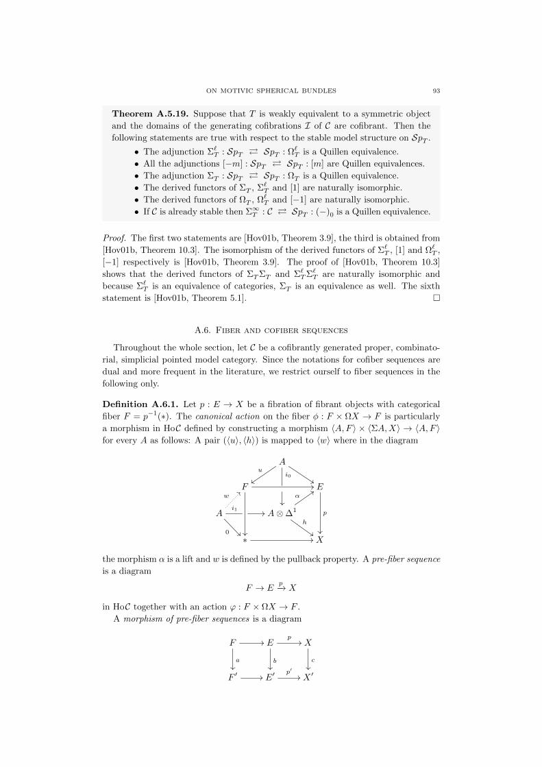
ON MOTIVIC SPHERICAL BUNDLES 93
Theorem A.5.19. Suppose that T is weakly equivalent to a symmetric object
and the domains of the generating cofibrations I of C are cofibrant. Then the
following statements are true with respect to the stable model structure on SpT .
• The adjunction Σ`T : SpT SpT : Ω`T is a Quillen equivalence.
• All the adjunctions [−m] : SpT SpT : [m] are Quillen equivalences.
• The adjunction ΣT : SpT SpT : ΩT is a Quillen equivalence.
• The derived functors of ΣT , Σ`T and [1] are naturally isomorphic.
• The derived functors of ΩT , Ω`T and [−1] are naturally isomorphic.
• If C is already stable then Σ∞T : C SpT : (−)0 is a Quillen equivalence.
Proof. The first two statements are [Hov01b, Theorem 3.9], the third is obtained from
[Hov01b, Theorem 10.3]. The isomorphism of the derived functors of Σ`T , [1] and Ω`T ,
[−1] respectively is [Hov01b, Theorem 3.9]. The proof of [Hov01b, Theorem 10.3]
shows that the derived functors of ΣTΣT and Σ`TΣ`T are naturally isomorphic and
because Σ`T is an equivalence of categories, ΣT is an equivalence as well. The sixth
statement is [Hov01b, Theorem 5.1].
A.6. Fiber and cofiber sequences
Throughout the whole section, let C be a cofibrantly generated proper, combinato-
rial, simplicial pointed model category. Since the notations for cofiber sequences are
dual and more frequent in the literature, we restrict ourself to fiber sequences in the
following only.
Definition A.6.1. Let p : E → X be a fibration of fibrant objects with categorical
fiber F = p−1(∗). The canonical action on the fiber φ : F × ΩX → F is particularly
a morphism in HoC defined by constructing a morphism 〈A,F 〉 × 〈ΣA,X〉 → 〈A,F 〉for every A as follows: A pair (〈u〉, 〈h〉) is mapped to 〈w〉 where in the diagram
A
i0$$
u
zzF
//
E
p
A
w??
0
i1 // A⊗∆1
h
$$
α::
∗ // X
the morphism α is a lift and w is defined by the pullback property. A pre-fiber sequence
is a diagram
F → Ep−→ X
in HoC together with an action ϕ : F × ΩX → F .
A morphism of pre-fiber sequences is a diagram
F
a
// E
b
p// X
c
F ′ // E′p′// X ′
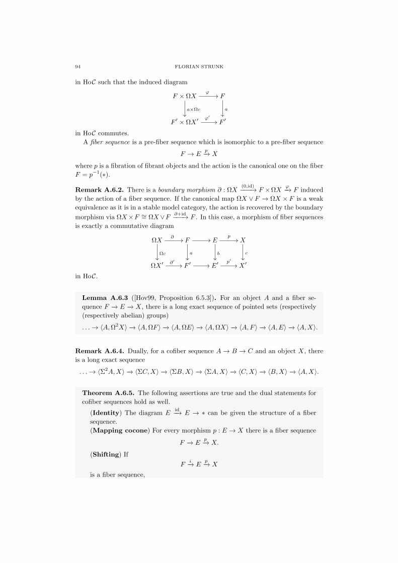
94 FLORIAN STRUNK
in HoC such that the induced diagram
F × ΩXϕ//
a×Ωc
F
a
F ′ × ΩX ′ϕ′// F ′
in HoC commutes.
A fiber sequence is a pre-fiber sequence which is isomorphic to a pre-fiber sequence
F → Ep−→ X
where p is a fibration of fibrant objects and the action is the canonical one on the fiber
F = p−1(∗).
Remark A.6.2. There is a boundary morphism ∂ : ΩX(0,id)−−−→ F ×ΩX
ϕ−→ F induced
by the action of a fiber sequence. If the canonical map ΩX ∨ F → ΩX × F is a weak
equivalence as it is in a stable model category, the action is recovered by the boundary
morphism via ΩX×F ∼= ΩX ∨F ∂+id−−−→ F . In this case, a morphism of fiber sequences
is exactly a commutative diagram
ΩX
Ωc
∂ // F
a
// E
b
p// X
c
ΩX ′∂′ // F ′ // E′
p′// X ′
in HoC.
Lemma A.6.3 ([Hov99, Proposition 6.5.3]). For an object A and a fiber se-
quence F −→ E −→ X, there is a long exact sequence of pointed sets (respectively
(respectively abelian) groups)
. . .→ 〈A,Ω2X〉 −→ 〈A,ΩF 〉 −→ 〈A,ΩE〉 −→ 〈A,ΩX〉 −→ 〈A,F 〉 −→ 〈A,E〉 −→ 〈A,X〉.
Remark A.6.4. Dually, for a cofiber sequence A → B → C and an object X, there
is a long exact sequence
. . .→ 〈Σ2A,X〉 −→ 〈ΣC,X〉 −→ 〈ΣB,X〉 −→ 〈ΣA,X〉 −→ 〈C,X〉 −→ 〈B,X〉 −→ 〈A,X〉.
Theorem A.6.5. The following assertions are true and the dual statements for
cofiber sequences hold as well.
(Identity) The diagram Eid−→ E → ∗ can be given the structure of a fiber
sequence.
(Mapping cocone) For every morphism p : E → X there is a fiber sequence
F −→ Ep−→ X.
(Shifting) If
Fi−→ E
p−→ X
is a fiber sequence,

ON MOTIVIC SPHERICAL BUNDLES 95
then there is a fiber sequence
ΩX∂−→ F
i−→ E.
(Extensibility) For every commutative diagram
Fi // E
p//
b
X
c
F ′i′ // E′
p′// X ′
in HoC, where the rows are fiber sequences, there exists a (not necessarily
unique) fill-in morphism a : F → F ′ defining together with b and c a morphism
of fiber sequences and particularly making the whole diagram commutative. If
b and c are isomorphisms, then so is a.
Proof. The first statement is [Hov99, Lemma 6.3.2]. The mapping cocone statement
is [Hov99, Lemma 6.3.3] and the shifting is [Hov99, Proposition 6.3.4]. The statement
on extensibility is [Hov99, Proposition 6.3.5] and [Hov99, Proposition 6.5.3].
Remark A.6.6. The non-uniqueness of the fill-in morphism in the extensibility state-
ment is closely related to the fact that a homotopy (co)limit is unique up to isomor-
phism in the homotopy category but not unique up to unique isomorphism although
this is true for categorical (co)limits.
The following lemma shows, that the work with fiber sequences is easier in right
proper model categories.
Lemma A.6.7. Let C be right proper. For a morphism p : E → X in HoC there
is up to isomorphism of fiber sequences only one fiber sequence
hofib −→ Ep−→ X.
Proof. The extensibility statement of Theorem A.6.5 shows the uniqueness and hence
we have only to show that there is a diagram
hofib −→ Ep−→ X
in HoC which can be furnished with the structure of a fiber sequence. Factorize a
representant in C of the HoC-morphism QE∼−→ E
p−→ X∼−→ RX as a acyclic cofibration
followed by a fibration. By Remark A.1.21, the categorical fiber of this fibration is a
homotopy fiber of p which uses the assumed right properness. One equips the diagram
hofib→ Ep−→ X with the action coming from the canonical action of this fibration.

96 FLORIAN STRUNK
References
[AD08] Aravind Asok and Brent Doran, Vector bundles on contractible smooth schemes, Duke
Mathematical Journal 143 (2008), no. 3, 513–530.
[Ada63] John Frank Adams, On the groups J(X). I, Topology 2 (1963), 181–195.
[Ada65a] , On the groups J(X). II, Topology 3 (1965), 137–171.
[Ada65b] , On the groups J(X). III, Topology 3 (1965), 193–222.
[Ada66] , On the groups J(X). IV, Topology 5 (1966), 21–71.
[AM11] Aravind Asok and Fabien Morel, Smooth varieties up to A1-homotopy and algebraic
h-cobordisms, Adv. Math. 227 (2011), no. 5, 1990–2058.
[AR94] Jiri Adamek and Jirı Rosicky, Locally presentable and accessible categories, London
Mathematical Society lecture note series ; 189, Cambridge Univ. Press, 1994.
[Ati61a] Michael Francis Atiyah, Characters and cohomology of finite groups, Inst. Hautes Etudes
Sci. Publ. Math. (1961), no. 9, 23–64.
[Ati61b] , Thom complexes, Proc. London Math. Soc. (3) 11 (1961), 291–310.
[Ayo07a] Joseph Ayoub, Les six operations de Grothendieck et le formalisme des cycles
evanescents dans le monde motivique. I, Asterisque (2007), no. 314, x+466 pp. (2008).
[Ayo07b] , Les six operations de Grothendieck et le formalisme des cycles evanescents dans
le monde motivique. II, Asterisque (2007), no. 315, vi+364 pp. (2008).
[Bar10] Clark Barwick, On left and right model categories and left and right Bousfield localiza-
tions, Homology, Homotopy Appl. 12 (2010), no. 2, 245–320.
[Bek00] Tibor Beke, Sheafifiable homotopy model categories, Math. Proc. Cambridge Philos. Soc.
129 (2000), no. 3, 447–475.
[BG75] James Cyril Becker and Daniel Henry Gottlieb, The transfer map and fiber bundles,
Topology 14 (1975), 1–12.
[Bla01] Benjamin Blander, Local Projective Model Structures on Simplicial Presheaves, K-
Theory 24 (2001), no. 3, 283–301.
[Bor91] Armand Borel, Linear algebraic groups, second ed., Graduate Texts in Mathematics,
vol. 126, Springer-Verlag, New York, 1991.
[Bor94a] Francis Borceux, Handbook of categorical algebra. 1, Encyclopedia of Mathematics and
its Applications, vol. 50, Cambridge University Press, Cambridge, 1994.
[Bor94b] , Handbook of categorical algebra. 2, Encyclopedia of Mathematics and its Ap-
plications, vol. 51, Cambridge University Press, Cambridge, 1994.
[Bor94c] , Handbook of categorical algebra. 3, Encyclopedia of Mathematics and its Ap-
plications, vol. 52, Cambridge University Press, Cambridge, 1994.
[Bot59] Raoul Bott, The stable homotopy of the classical groups, Ann. of Math. (2) 70 (1959),
313–337.
[Bro73] Edgar Brown, A proof of the Adams conjecture, Unpublished, 1973.
[BV68] John Michael Boardman and Rainer M. Vogt, Homotopy-everything H-spaces, Bull.
Amer. Math. Soc. 74 (1968), 1117–1122.
[CH02] John Daniel Christensen and Mark Hovey, Quillen model structures for relative homo-
logical algebra, Mathematical Proceedings of the Cambridge Philosophical Society, vol.
133, Cambridge Univ Press, 2002, pp. 261–293.
[CP97] Jean-Marc Cordier and Timothy Porter, Homotopy coherent category theory, Trans.
Amer. Math. Soc. 349 (1997), no. 1, 1–54.
[CS06] David Chataur and Jerome Scherer, Fiberwise localization and the cube theorem, Com-
ment. Math. Helv. 81 (2006), no. 1, 171–189.
[DG70] Michel Demazure and Pierre Gabriel, Groupes algebriques. Tome I: Geometrie
algebrique, generalites, groupes commutatifs, Masson & Cie, Editeur, Paris, 1970, Avec
un appendice Corps de classes local par Michiel Hazewinkel.
[DHI04] Daniel Dugger, Sharon Hollander, and Daniel C. Isaksen, Hypercovers and simplicial
presheaves, Math. Proc. Cambridge Philos. Soc. 136 (2004), no. 1, 9–51.
[DHKS04] William Gerard Dwyer, Philip Steven Hirschhorn, Daniel Marinus Kan, and Jeffrey Hen-
derson Smith, Homotopy Limit Functors on Model Categories and Homotopical Cate-
gories, Mathematical Surveys and Monographs, vol. 113, American Mathematical Soci-
ety, 2004.
ON MOTIVIC SPHERICAL BUNDLES 97
[Doe98] Jean-Paul Doeraene, Homotopy pull backs, homotopy push outs and joins, Bull. Belg.
Math. Soc. Simon Stevin 5 (1998), no. 1, 15–37.
[Dol94] Igor V. Dolgachev, Introduction to geometric invariant theory, Lecture Notes Series,
vol. 25, Seoul National University Research Institute of Mathematics Global Analysis
Research Center, Seoul, 1994.
[DRØ03a] Bjørn Ian Dundas, Oliver Rondigs, and Paul Arne Østvær, Enriched functors and stable
homotopy theory, Documenta Mathematica 8 (2003), 409–488.
[DRØ03b] Bjørn Ian Dundas, Oliver Rondigs, and Paul Arne Østvær, Motivic Functors, Docu-
menta Mathematica 8 (2003), 489–525.
[Dug98] Daniel Dugger, Sheaves and Homotopy Theory, Unpublished, 1998.
[Dug01] , Replacing model categories with simplicial ones, Trans. Amer. Math. Soc. 353
(2001), no. 12, 5003–5027.
[Ebe] Johannes Ebert, The Adams Conjecture, after Edgar Brown, Unpublished.
[Fau06] Halvard Fausk, T -model structures on chain complexes of presheaves, Preprint, 2006.
[Fri73] Eric M. Friedlander, Fibrations in etale homotopy theory, Inst. Hautes Etudes Sci. Publ.
Math. (1973), no. 42, 5–46.
[Gam10] Nicola Gambino, Weighted limits in simplicial homotopy theory, J. Pure Appl. Algebra
214 (2010), no. 7, 1193–1199.
[GJ99] Paul Gregory Goerss and John Frederick Jardine, Simplicial Homotopy Theory, Progress
in Mathematics, vol. 174, Birkhauser, 1999.
[GLMS+00] B. Brent Gordon, James D. Lewis, Stefan Muller-Stach, Shuji Saito, and Noriko Yui
(eds.), The arithmetic and geometry of algebraic cycles, NATO Science Series C: Math-
ematical and Physical Sciences, vol. 548, Kluwer Academic Publishers, 2000.
[Gro61] Alexander Grothendieck, Elements de geometrie algebrique. II. Etude globale
elementaire de quelques classes de morphismes, Inst. Hautes Etudes Sci. Publ. Math.
(1961), no. 8, 222.
[Gro67] , Elements de geometrie algebrique. IV. Etude locale des schemas et des mor-
phismes de schemas IV, Inst. Hautes Etudes Sci. Publ. Math. (1967), no. 32, 361.
[GW10] Ulrich Gortz and Torsten Wedhorn, Algebraic Geometry: Part I: Schemes. With Exam-
ples and Exercises, vol. 1, Vieweg+Teubner Verlag, 2010.
[Hab75] William J. Haboush, Reductive groups are geometrically reductive, Ann. of Math. (2)
102 (1975), no. 1, 67–83.
[Hir03] Philip Steven Hirschhorn, Model Categories and Their Localizations, Mathematical Sur-
veys and Monographs, American Mathematical Society, 2003.
[Hir05] , Overcategories and Undercategories of Model Categories, Unpublished, 2005.
[Hor06] Jens Hornbostel, Localizations in motivic homotopy theory, Math. Proc. Camb. Phil.
Soc. 140 (2006), no. 95, 95–114.
[Hov99] Mark Hovey, Model Categories, Mathematical Surveys and Monographs, vol. 63, Amer-
ican Mathematical Society, 1999.
[Hov01a] , Model category structures on chain complexes of sheaves, Trans. Amer. Math.
Soc. 353 (2001), no. 6, 2441–2457.
[Hov01b] , Spectra and symmetric spectra in general model categories, J. Pure Appl. Al-
gebra 165 (2001), no. 1, 63–127.
[HS09] Philip Herrmann and Florian Strunk, Simplicial Functors and Motivic Homotopy The-
ory, Unpublished, 2009.
[Hu01] Po Hu, Base change functors in the A1-stable homotopy category., Homology, Homotopy
and Applications 3 (2001), no. 2, 417–451.
[Hu05] , On the Picard group of the stable A1-homotopy category, Topology 44 (2005),
no. 3, 609–640.
[Jan87] Jens Carsten Jantzen, Representations of algebraic groups, Pure and Applied Mathe-
matics, vol. 131, Academic Press Inc., Boston, MA, 1987.
[Jar87] John Frederick Jardine, Simplicial presheaves, Journal of Pure and Applied Algebra 47
(1987), no. 1, 35–87.
[Jar96] , Boolean localization, in practice, Doc. Math. 1 (1996), No. 13, 245–275.
[Jar00a] , Motivic Symmetric Spectra, Documenta Mathematica 5 (2000), 445–552.
[Jar00b] , Presheaves of symmetric spectra, J. Pure Appl. Algebra 150 (2000), no. 2,
137–154.

98 FLORIAN STRUNK
[Jar03] , Presheaves of chain complexes, K-theory 30 (2003), no. 4, 365–420.
[Jar11] , Local Homotopy Theory, Preprint, 2011.
[Joh02] Peter Tennant Johnstone, Sketches of an elephant: a topos theory compendium. Vol. 1,
Oxford Logic Guides, vol. 43, The Clarendon Press Oxford University Press, New York,
2002.
[Joy84] Andre Joyal, Letter to Alexander Grothendieck, 1984.
[Lan02] Serge Lang, Algebra, third ed., Graduate Texts in Mathematics, vol. 211, Springer-
Verlag, New York, 2002.
[Lew91] LeMoine Gaunce Jr. Lewis, Is there a convenient category of spectra?, J. Pure Appl.
Algebra 73 (1991), no. 3, 233–246.
[Liu02] Qing Liu, Algebraic Geometry and Arithmetic Curves, Oxford Graduate Texts in Math-
ematics, Oxford University Press, 2002.
[LS06] Stephen Lack and Pawe l Sobocinski, Toposes are adhesive, Graph transformations, Lec-
ture Notes in Comput. Sci., vol. 4178, 2006, pp. 184–198.
[Lur09] Jacob Lurie, Higher topos theory, Annals of mathematics studies 170, Princeton Univ.
Press, 2009.
[Mat76] Michael Mather, Pull-backs in homotopy theory, Canad. J. Math. 28 (1976), no. 2,
225–263.
[May95] Jon Peter May, Equivariant stable homotopy theory, Handbook of Algebraic Topology
(1995), 277.
[May01a] , Picard groups, Grothendieck rings, and Burnside rings of categories, Advances
in Mathematics 163 (2001), no. 1, 1–16.
[May01b] , The additivity of traces in triangulated categories, Advances in Mathematics
163 (2001), no. 1, 34–73.
[MFK94] David Mumford, John Charde Fogarty, and Frances Clare Kirwan, Geometric invari-
ant theory, third ed., Ergebnisse der Mathematik und ihrer Grenzgebiete (2), vol. 34,
Springer-Verlag, Berlin, 1994.
[Mil80] James Stuart Milne, Etale Cohomology, Princeton Mathematical Series, vol. 33, Prince-
ton University Press, 1980.
[MM92] Saunders Mac Lane and Ieke Moerdijk, Sheaves in Geometry and Logic, Universitext,
Springer, 1992.
[Mor04] Fabien Morel, On the motivic π0 of the sphere spectrum, Axiomatic, enriched and mo-
tivic homotopy theory (2004), 219–260.
[Mor12] , A1-Algebraic topology over a field, Preprint, 2012.
[MV99] Fabien Morel and Vladimir Voevodsky, A1-homotopy theory of schemes, Publications
Mathematiques de l’Institut des Hautes Etudes Scientifiques 90 (1999), 45–143.
[MVW06] Carlo Mazza, Vladimir Voevodsky, and Charles Weibel, Lecture notes on motivic coho-
mology, Clay Mathematics Monographs, vol. 2, American Mathematical Society, Provi-
dence, RI, 2006.
[Nis87] Yevsey A. Nisnevich, The completely decomposed topology on schemes and associated
descent spectral sequences in algebraic K-theory, Algebraic K-theory: connections with
geometry and topology (Lake Louise, AB), NATO Adv. Sci. Inst. Ser. C Math. Phys.
Sci., vol. 279, 1987, pp. 241–342.
[PPR07] Ivan A. Panin, Konstantin Pimenov, and Oliver Rondigs, On Voevodsky’s algebraic K-
theory spectrum BGL, Preprint, http://arxiv.org/pdf/0709.3905 (2007).
[Qui71] Daniel Quillen, The Adams conjecture, Topology 10 (1971), 67–80.
[Rez98] Charles Rezk, Fibrations and homotopy colimits of simplicial sheaves, Preprint, 1998.
[Rez10] , Toposes and Homotopy Toposes, Preprint, 2010.
[RØ06] Oliver Rondigs and Paul Arne Østvær, Motives and modules over motivic cohomology,
C. R. Math. Acad. Sci. Paris 342 (2006), no. 10, 751–754.
[Ron05] Oliver Rondigs, Functoriality in motivic homotopy theory, Unpublished, 2005.
[Ron10] , Theta characteristics and stable homotopy types of curves, Q. J. Math. 61
(2010), no. 3, 351–362.
[Rud98] Yuli B. Rudyak, On Thom spectra, orientability, and cobordism, Springer Monographs
in Mathematics, Springer-Verlag, Berlin, 1998, With a foreword by Haynes Miller.
[Sch11] Urs Schreiber, Differential cohomology in a cohesive topos, Habilitation, Hamburg, 2011.
ON MOTIVIC SPHERICAL BUNDLES 99
[Shu09] Michael Shulman, Homotopy limits and colimits and enriched homotopy theory,
Preprint, 2009.
[Skj09] Roy Mikael Skjelnes, Algebraic spaces and quotients by equivalence relation of schemes,
Preprint, 2009.
[SØ10] Markus Spitzweck and Paul Arne Østvær, Motivic twisted K-theory, Preprint, 2010.
[Spa88] Nicolas Spaltenstein, Resolutions of unbounded complexes, Compositio Math. 65 (1988),
no. 2, 121–154.
[Sta63] James Stasheff, A classification theorem for fibre spaces, Topology 2 (1963).
[Str11] Jeffrey Strom, Modern classical homotopy theory, Graduate Studies in Mathematics,
vol. 127, American Mathematical Society, Providence, RI, 2011.
[Sul74] Dennis Sullivan, Genetics of homotopy theory and the Adams conjecture, Ann. of Math.
(2) 100 (1974), 1–79.
[Toe09] Bertrand Toen, Simplicial presheaves and derived algebraic geometry, Advanced Course
on Simplicial Methods in Higher Categories [46], Notes of the Course (2009), 95–146.
[TT90] Robert Wayne Thomason and Thomas Trobaugh, Higher algebraic K-theory of schemes
and of derived categories, The Grothendieck Festschrift, Vol. III, Progr. Math., vol. 88,
1990, pp. 247–435.
[TV07] Bertrand Toen and Michel Vaquie, Moduli of objects in dg-categories, Ann. Sci. Ecole
Norm. Sup. (4) 40 (2007), no. 3, 387–444.
[Voe97] Vladimir Voevodsky, The Milnor conjecture, 1997.
[Voe10] , Unstable motivic homotopy categories in Nisnevich and cdh-topologies, J. Pure
Appl. Algebra 214 (2010), no. 8, 1399–1406.
[Wei94] Charles Weibel, An introduction to homological algebra, Cambridge Studies in Advanced
Mathematics, vol. 38, Cambridge University Press, Cambridge, 1994.
[Wei12] , An introduction to algebraic K-theory, 2012, Unpublished.
[Wen07] Matthias Wendt, On Fibre Sequences in Motivic Homotopy Theory, Dissertation, 2007.
[Wen10] , Classifying spaces and fibrations of simplicial sheaves, Unpublished, 2010.
[Wen11] , Rationally trivial torsors in A1-homotopy theory, J. K-Theory 7 (2011), no. 3,
541–572.
[Whi42] George W. Whitehead, On the homotopy groups of spheres and rotation groups, Ann.
of Math. (2) 43 (1942), 634–640.