flow-based segmentation of seismic data -...

Flow-based Segmentation of Seismic Data

Kari Ringdal∗

Supervised by: Daniel Patel†

Institute of InformaticsUniversity of Bergen

Bergen / Norway

Abstract

This paper presents an image processing method for iden-tifying separate layers in seismic 3D reflection volumes.This is done by applying techniques from flow visualiza-tion and using GPU acceleration. Sound waves are usedfor exploring the earth beneath the surface. The result-ing seismic data gives us a representation of sedimentaryrocks. Analysing sedimentary rocks and their layering canreveal major historical events, such as earth crust move-ment, climate change or evolutionary change. Sedimen-tary rocks are also important as a source of natural re-sources like coal, fossil fuels, drinking water and ores. Thefirst step in analysing seismic reflection data is to find theborders between sedimentary units that originated at dif-ferent times. This paper presents a technique for detectingseparating borders in 3D seismic data. Layers belonging todifferent units can not always be detected on a local scale.Our presented technique avoids the shortcoming of exist-ing methods working on a local scale by addressing thedata globally. We utilize methods from the fields of flowvisualization and image processing. We describe a bor-der detection algorithm, as well as a general programmingpipeline for preprocessing the data on the graphics card.Our GPU processing supports fast filtering of the data anda real-time update of the viewed volume slice when pa-rameters are adjusted.

Keywords: Seismic Data, Structure Extraction, GPU-accelerated Image Processing

1 Introduction

Stratigraphy is the study of rock layers deposited in theearth. A stratum (plural: strata) can be defined as a homo-geneous bed of sedimentary rock. Stratigraphy has been ageological discipline ever since the 17th century, and waspioneered by the Danish geologist Nicholas Steno (1638-1686). He reasoned that rock strata were formed whenparticles in a fluid, such as water, fell to the bottom [10].The particles would settle evenly in horizontal layers on alake or ocean floor. Through all of Earth’s history, layers

∗[email protected]†[email protected]

of sedimentary rock have been formed as wind, water orice has deposited organic and mineral matter into a body ofwater. The matter has sunk to the bottom and consolidatedinto rock by pressure and heat. A break in the continuousdeposit results in an unconformity, in other words, the sur-face where successive layers of sediments from differenttimes meet. An unconformity represents a gap in the ge-

Figure 1: Stratified sediments. The sedimentary facies areseparated by unconformities.

ological record. It usually occurs as a response to changein the water or sea level. Lower water levels expose stratato erosion, and a rise in the water level may cause newhorizontal layers of deposition to resurge on top of theolder truncated layers. The geologists analyse the patternaround an unconformity to decode the missing time it rep-resents. Above and below an unconformity there are two

Figure 2: Strata relates to an unconformity in differentways. The top three images show patterns that occur be-low an unconformity, and the bottom three images showpatterns that occur above an unconformity.

types of terminating patterns and one non-terminating pat-

Proceedings of CESCG 2012: The 16th Central European Seminar on Computer Graphics (non-peer-reviewed)

tern. Truncation and toplap terminates at the unconformityabove. Truncation is mainly a result of erosion and toplapis a result of non-deposition. Strata above an unconformitymay terminate in the pattern of onlap or downlap. On-lap happens when the horizontal strata terminates againsta base with greater inclination, and downlap is seen whereyounger non-horizontal layers terminates against the un-conformity below. Concordance can occur both above andbelow an unconformity and is where the strata layers areparallel to the unconformity. An illustration of these con-cepts can be seen in Figure 2.

An unconformity can be traced into its correlative con-formity. In contrast to an unconformity, there is no evi-dence of erosion or non-deposition along the conformity.

Figure 3: Sediments ofdifferent facies can beindistinguishable in lo-cal areas such as insidethe circle.

A seismic sequence - alsocalled a sedimentary unit orfacies, is delimited by uncon-formities and their correlativeconformities. The fact thatsediments belonging to dif-ferent seismic sequences canbe indistinguishable in greaterparts of the picture, as illus-trated in Figure 3, calls forglobal analysing tools.

For more information onunconformities, sedimentarysequences and other strati-graphic concepts, the reader is

referred to Nichols book on sedimentology and stratigra-phy [13] and Catuneaus book on sequence stratigraphy [4].

Many techniques to highlight interesting attributes inseismic data have been developed [6]. Taner [17] gives auseful definition of seismic attributes: “Seismic Attributesare all the information obtained from seismic data, eitherby direct measurement or by logical or experience basedreasoning”. Dip and azimuth are attributes that describethe dominating orientation of the strata locally. Dip givesthe vertical angle and azimuth the lateral angle.

In our work, we consider the dip/azimuth vectors to con-stitute a flow field representation of the data set where theflow “moves” along the sediment layers. We seed parti-cles from neighbouring points in this flow, and considerthe distances between the end points of the generated tra-jectories. A great distance gives a high probability that theseed point is a surface point. Mapped surface points arethen linked to constitute unconformity surfaces. Figure 4gives an overview of our processing pipeline.

2 Related Work

Interpreting seismic data is a time consuming task, andextensive work has been done to automate this. This sec-tion will focus on previous approaches on finding uncon-formities, and also look into methods within the fields ofimage processing and flow visualization that relates to the

new technique presented in this paper. Orientation fieldextraction from image processing relates to vector field ex-traction of seismic data. Image processing also deals withedge linking methods, which relates to the segmentationprocess of our method. The field of flow visualization usemethods relevant to the mapping of surface probability.

2.1 Seismic methods

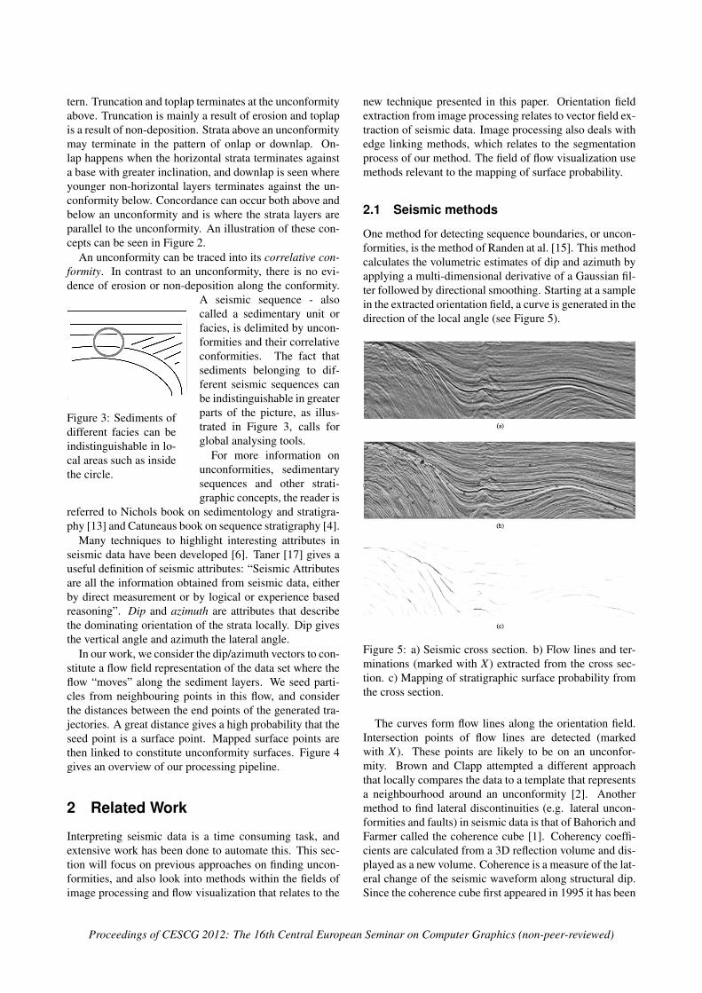
One method for detecting sequence boundaries, or uncon-formities, is the method of Randen at al. [15]. This methodcalculates the volumetric estimates of dip and azimuth byapplying a multi-dimensional derivative of a Gaussian fil-ter followed by directional smoothing. Starting at a samplein the extracted orientation field, a curve is generated in thedirection of the local angle (see Figure 5).

Figure 5: a) Seismic cross section. b) Flow lines and ter-minations (marked with X) extracted from the cross sec-tion. c) Mapping of stratigraphic surface probability fromthe cross section.

The curves form flow lines along the orientation field.Intersection points of flow lines are detected (markedwith X). These points are likely to be on an unconfor-mity. Brown and Clapp attempted a different approachthat locally compares the data to a template that representsa neighbourhood around an unconformity [2]. Anothermethod to find lateral discontinuities (e.g. lateral uncon-formities and faults) in seismic data is that of Bahorich andFarmer called the coherence cube [1]. Coherency coeffi-cients are calculated from a 3D reflection volume and dis-played as a new volume. Coherence is a measure of the lat-eral change of the seismic waveform along structural dip.Since the coherence cube first appeared in 1995 it has been


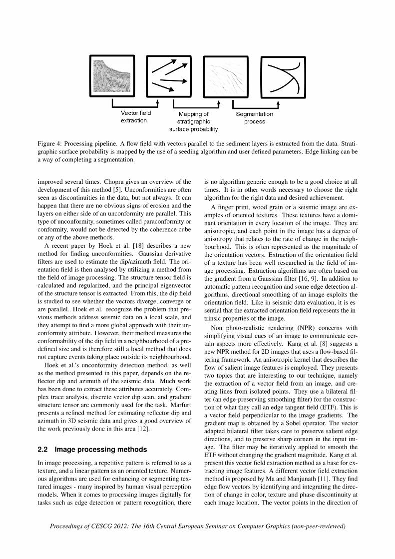
Figure 4: Processing pipeline. A flow field with vectors parallel to the sediment layers is extracted from the data. Strati-graphic surface probability is mapped by the use of a seeding algorithm and user defined parameters. Edge linking can bea way of completing a segmentation.

improved several times. Chopra gives an overview of thedevelopment of this method [5]. Unconformities are oftenseen as discontinuities in the data, but not always. It canhappen that there are no obvious signs of erosion and thelayers on either side of an unconformity are parallel. Thistype of unconformity, sometimes called paraconformity orconformity, would not be detected by the coherence cubeor any of the above methods.

A recent paper by Hoek et al. [18] describes a newmethod for finding unconformities. Gaussian derivativefilters are used to estimate the dip/azimuth field. The ori-entation field is then analysed by utilizing a method fromthe field of image processing. The structure tensor field iscalculated and regularized, and the principal eigenvectorof the structure tensor is extracted. From this, the dip fieldis studied to see whether the vectors diverge, converge orare parallel. Hoek et al. recognize the problem that pre-vious methods address seismic data on a local scale, andthey attempt to find a more global approach with their un-conformity attribute. However, their method measures theconformability of the dip field in a neighbourhood of a pre-defined size and is therefore still a local method that doesnot capture events taking place outside its neighbourhood.

Hoek et al.’s unconformity detection method, as wellas the method presented in this paper, depends on the re-flector dip and azimuth of the seismic data. Much workhas been done to extract these attributes accurately. Com-plex trace analysis, discrete vector dip scan, and gradientstructure tensor are commonly used for the task. Marfurtpresents a refined method for estimating reflector dip andazimuth in 3D seismic data and gives a good overview ofthe work previously done in this area [12].

2.2 Image processing methods

In image processing, a repetitive pattern is referred to as atexture, and a linear pattern as an oriented texture. Numer-ous algorithms are used for enhancing or segmenting tex-tured images - many inspired by human visual perceptionmodels. When it comes to processing images digitally fortasks such as edge detection or pattern recognition, there

is no algorithm generic enough to be a good choice at alltimes. It is in other words necessary to choose the rightalgorithm for the right data and desired achievement.

A finger print, wood grain or a seismic image are ex-amples of oriented textures. These textures have a domi-nant orientation in every location of the image. They areanisotropic, and each point in the image has a degree ofanisotropy that relates to the rate of change in the neigh-bourhood. This is often represented as the magnitude ofthe orientation vectors. Extraction of the orientation fieldof a texture has been well researched in the field of im-age processing. Extraction algorithms are often based onthe gradient from a Gaussian filter [16, 9]. In addition toautomatic pattern recognition and some edge detection al-gorithms, directional smoothing of an image exploits theorientation field. Like in seismic data evaluation, it is es-sential that the extracted orientation field represents the in-trinsic properties of the image.

Non photo-realistic rendering (NPR) concerns withsimplifying visual cues of an image to communicate cer-tain aspects more effectively. Kang et al. [8] suggests anew NPR method for 2D images that uses a flow-based fil-tering framework. An anisotropic kernel that describes theflow of salient image features is employed. They presentstwo topics that are interesting to our technique, namelythe extraction of a vector field from an image, and cre-ating lines from isolated points. They use a bilateral fil-ter (an edge-preserving smoothing filter) for the construc-tion of what they call an edge tangent field (ETF). This isa vector field perpendicular to the image gradients. Thegradient map is obtained by a Sobel operator. The vectoradapted bilateral filter takes care to preserve salient edgedirections, and to preserve sharp corners in the input im-age. The filter may be iteratively applied to smooth theETF without changing the gradient magnitude. Kang et al.present this vector field extraction method as a base for ex-tracting image features. A different vector field extractionmethod is proposed by Ma and Manjunath [11]. They findedge flow vectors by identifying and integrating the direc-tion of change in color, texture and phase discontinuity ateach image location. The vector points in the direction of


the closest boundary pixel.Edge linking is another area from image processing that

is relevant to our method. An image of unconformity linesmay contain gaps, and with an ultimate goal of segmen-tation, proper linking of edges is necessary. Fundamen-tal approaches to edge linking concern both local process-ing where knowledge about edge points in a local regionis required, and regional processing where points on theboundary of a region must be known [7]. There are alsoglobal processing methods, like the Hough transform. ForKang et al.’s flow-based image abstraction method [8],part of the goal is to end up with an image-guided 2Dline drawing. Here the lines are generated by steering aDoG (difference of Gaussian) edge detection filter alongthe ETF flow and accumulate the information. This way,the quality of lines is enhanced. (see Figure 6).

Figure 6: Edge linking. a) Input image. b) Filtered byDoG filter. c) Filtered by Kang et al.’s flow-based DoGfilter.

2.3 Flow field topology and extraction meth-ods

Flow visualization is a sub-field of data visualization thatdevelops methods to make flow patterns in fluids visible.Flow features and techniques for topology extraction ofsteady vector field data will be the focus of this section. Afeature is a structure or an object of interest. Shock waves,vortices, boundary layers, recirculation zones, and attach-ment and separation lines are examples of flow features.

Relating flow to seismic data, features that are mostlikely to occur in a vector field extracted from seismic dataare separation and attachment lines, this because of theonlap, toplap and downlap terminations. Separation andattraction lines are lines on the boundary of a body of aflow where the flow abruptly moves away from or returnsto the surface of the flow body. A state of the art reportby Post et al. [14] deals with different methods for sep-aration and attachment line extraction. Methods for bothopen and closed separation are discussed. One approachmentioned is particle seeding and computation of integralcurves. A particle is released into the flow field and itspath is found by integrating the vector field (that repre-sents the flow field) along a curve. If we look at the vectorfield extracted from seismic data as a flow field, we have asteady flow. The fact that it is not time-dependent meansthat the pathline of a seeded particle is everywhere tangentto the vectors of the flow. According to the aim of this pa-

per, feature extraction and its instrumental algorithms areof greater interest than the actual visualization of the data.We will not use pathlines for visualization purposes, but asa tool in addressing the seismic data on a global scale.

3 Implementation Details

Our method for separating the sedimentary units in 3Dseismic data follows the processing pipeline shown in Fig-ure 4. The processing steps are separated into three cate-gories:

• Vector field extraction from the seismic data

• Mapping of stratigraphic surface probability

• Segmentation process

This section will take a closer look at each of the steps, butfocus on the second step of the pipeline - the mapping ofstratigraphic surface probability using concepts from flow.In this step lies the novelty of our method.

3.1 Preprocessing - vector field extractionon the GPU

As described in the Related work section, there already ex-ists efficient methods for estimating the reflector dip andazimuth of seismic data. The extraction of this vector fieldis an important step of the pipeline, because a regular vec-tor field, that represents the data accurately, is crucial toour technique. The idea is to apply our unconformity ex-traction algorithm on a dip/azimuth vector field found byalready established methods. For testing the algorithm wehave created 2D and 3D synthetic data sets and imple-mented image processing methods for extracting the vec-tor field. The 3D data sets were created either by stackingan image to form a volume or by procedurally creating avolume of vectors pointing in different directions on eitherside of a delimiting surface. Only the last mentioned typeof test set has a variation in z-direction. The test sets havebeen useful for testing our algorithm and for getting a feelof the vector field extraction calculations which were donein parallel on a graphics card. The implemented program-ming pipeline is transferable to real seismic data volumes.

The highly parallel structure of modern GPUs is idealfor efficiently processing large blocks of data provided thecalculations could be done in parallel. GPUs support pro-grammable shaders that manipulate geometric vertices andfragments and output a color for every pixel on the screen.Instead of output to the screen, the RGBA-vectors can bewritten to 2D or 3D textures. A texture is in this sense ablock of memory located on the GPU where every point ofthe texture is a four dimensional vector. GPU-acceleratedmethods are rapidly expanding within the oil and gas in-dustry, and have dramatically increased the computing per-formance on seismic data.


For our implementation, we have used the OpenGLAPI and the OpenGL shading language GLSL within theframework of Volumeshop [3]. The programmed pipelinedoes GPU filtering of 3D data iteratively with a real-timeupdate of the viewed 2D slice when adding, removing oradjusting any of the filters. This allows a fine-tuning ofparameters before the entire data volume is processed.

The volume is loaded on the GPU in a 3D texture. GPU-memory is reserved for two more textures of equal size asthe volume, and the original texture is copied to one ofthem. The two textures are used alternately for readingand writing in a ping-pong fashion while the desired num-ber of filters is applied. The different filters are written asshaders in a plugin. Any number of this plugin is addedto the Volumeshop interface. They all operate on the GPUby having one plugin for every filter applied to the volume.The user chooses a filter from a pull down menu, and the

Figure 7: The data is loaded onto the GPU memory in a3D texture. Data is alternately read and written betweentwo more textures in a ping-pong fashion while filters areapplied iteratively. The data is filtered in parallel on theGPU, and a flow field representing the data is extracted.Output from a filter is rendered to the ping or pong tex-tures. Any output slice can also be rendered to the display.

filter parameters can be adjusted by sliders. It is also pos-sible to choose how many slices of the volume are filteredat each step. This way 3D filtering can be done on a sub-set of the volume to quickly assess the result. Adjustmentsof a filter leads to reprocessing of the data from the orig-inal volume through all the added filters. Therefore, theoriginal volume is kept as a separate texture on the GPUand not overwritten as the ping-pong textures. Figure 7

illustrates the implementation. All calculations are savedwith floating point precision in the RGBA-vectors of the3D textures. Results can be visualised directly by render-ing the RGBA-vectors to the screen, i.e. a flow field is seenas colors that varies according to the dip/azimuth vectors.This gives a good indication of the effect of each appliedfilter. A flow field represented as colors can be seen inColour plate Figure 12 b).

3.2 Mapping of stratigraphic surface proba-bility

Our unconformity detection algorithm is implemented asa shader, and calculations are done in parallel on the GPU.The technique uses particle seeding, as is common in thefield of flow visualization, but the paths of the particles arenot visualized. We use particle seeding from four neigh-bouring points to check whether they belong to the samesedimentary unit or not. The algorithm is as follows: Forevery point on a volume slice, four seed points are cho-sen. The seed points have coordinates (x,y,z), (x+d,y,z),(x,y + d,z) and (x,y,z + d). d is set so all four pointsare within a local neighbourhood. The seeding is calcu-lated by sampling the flow from the 3D texture using theRunge Kutta 4th order (RK4) method. All four paths arefollowed until a user- defined number of steps are taken, orthe path reaches coordinates outside of the volume-texture.The distances between the four end points are calculated.

Figure 8: Illustration ofthe border detection al-gorithm. The dots rep-resents three seeds thatmove along paths in aflow field. If the dis-tance between the path-ends exceeds a threshold,a probable surface point ismarked.

If a distance greater thana user-defined thresholdis detected, the originalseed point with coordi-nates (x,y,z) is marked asa probable point on an un-conformity. Figure 8 isan illustration of the al-gorithm in 2D. It is ex-pected that a great distanceindicate that the particleshave moved along differ-ently shaped paths. Be-cause of the parallel natureof the seismic data, twoclose paths will end up inthe same neighbourhood iftheir seed points are withinthe same sedimentary unit.We use four seed points todetect borders of any an-gle. The advantage of this method is that paths of manysteps address the data globally and unconformities canbe mapped even with parallel horizons on both sides. Apremise is that the particles move into a non-parallel areaalong their paths.

Since the algorithm is implemented as a shader, it is ex-ecuted in parallel for every pixel of the rendered region.The rectangular viewing region is set to correspond to the


width and height of the volume, and this region is ren-dered to the screen or directly to the ping-pong textures.The user can adjust the number of path steps and the dis-tance threshold used by the algorithm. The effect of ad-justing these parameters is seen in real-time on one sliceof the volume. When the desired parameter values are set,the rest of the volume is processed, slice-by-slice, with thesame settings. This way, the seeding algorithm is executedfor every vertex in the volume.

When the flow field is sampled from the 3D texture dur-ing the path calculations, OpenGL takes care of any neces-sary interpolation. The textures are set up for trilinear in-terpolation, and the paths are found by the RK4 integrationmethod. If the step size of this method is set to h, the errorper step is on the order of h5, while the total accumulatederror has order h4. Because of the error accumulation, asmall step size is desirable. The step size together with thenumber of steps affect whether the implemented techniqueis run locally or globally. Since the RK4 calculations area bottleneck in our technique, the balancing between theaccuracy of the method and the performance speed lies inthe choice of these parameters. We are using a step size of0.5. The number of steps is chosen in the user interface.

Ideally, the mapped points constitute unconformity lineswithout gaps when the seeding is done for every point ona slice, and unconformity surfaces without gaps when theseeding is done on the entire volume. However, this israre, when dealing with real seismic data, and some frag-mentation and false positives may occur. We have takensome measures to reduce misclassification. For more ro-bustness of the algorithm we perform the seeding in bothdirections of the flow. We also scale the endpoint distancesby the number of path steps to makes sure that a path offew steps will be as sensitive to the given threshold as apath of many steps. To avoid false positives, comparedparticle paths are discarded if their paths have a great vari-ation in the executed number of steps.

3.3 The segmentation process

The ultimate goal is a fully automated segmentation ofseismic data into sedimentary units. However, when run-ning the algorithm on noisy data, some fragmentation ofthe detected borders may occur. In that case, edge linkingis required. This step is not implemented at the currentstage, as it is not the main focus of this work. See theend of Section 2.2 for possible methods to achieve edgelinking.

4 Results / Application

To test the idea behind the presented technique, 2D and3D test sets were generated. The first 2D test set of size256× 256 is a vector field that simulates the flow field oftwo sedimentary units with parallel layers in greater partsof the picture. As expected, the unconformity surface was

Figure 9: 2D test set of size 256× 256 representing thevector field from two sedimentary units. a) The border de-tection algorithm is run locally - each particle is followedfor 20 steps, and only a part of the border is detected. b)The algorithm is run globally - each particle is followedfor 200 steps, and the border is detected throughout thedata set.

only found in the area without parallel layers when the al-gorithm was run locally (see Figure 9a). Each particle pathhad 20 steps with a step size of 1 which means that everyparticle travelled within a local neighbourhood. Figure 9bshows the result of increasing the number of steps to 200.Now the unconformity was mapped all the way, also in thearea of parallel layers.

The second test set is a 3D vector field of size 256×256×256. It also simulates two sedimentary units. Figure10 a) shows the flow field on a slice of the volume. Thetwo units have vectors with different z-components andthe data set varies in depth. The seeding algorithm wasrun on this flow field with 100 path steps and a step size of0.5, and the unconformity surface was found. Figure 10bshows the detected surface displayed in VoulmeShop. Onthis simple test set, the algorithm has generated a completesurface, and edge linking is not required.

For test set number 3 we used an image of a seismicdata slice from Randen et al.‘s article [15], and stackedcopies of this image to create a 3D volume. The result-ing volume is of size 256×256×256. This data set doesnot vary in depth as a seismic volume, but it gives us a


Figure 10: Test set 2 is a 3D vector field. a) A slice of thevolume with lines following the flow field. b) A volumet-ric representation of the surface extracted by the borderdetection algorithm.

way to test our vector field extraction filters and 3D fil-tering in real-time. Four filters were applied to the testset. Gradients were calculated by central difference androtated 90 degrees clockwise around the z-axis. Flow vec-tors with a negative x-component were turned 180 degrees.Then a Gaussian blur filter was used before a median filtersmoothed the flow field even more. At last we applied thefilter that contains the border detection algorithm. The re-sult is seen in Figure 11, and shows that some borders aredetected also in places where the layers appear parallel.

The last test set is again generated from stacking copiesof an image. We used an image that represents a seismicimage picturing many sedimentary units (Colour plate Fig-ure 12a). The data set is of size 512×512×64. First theflow vectors were found by central difference as with testset number 3. Then the flow field was smoothed by Kang

et al.‘s bilateral smoothing filter [8] reviewed in Section2.2. Also, a 3× 3 mean filter was used for more smooth-ing. All vectors were normalized. Colour plate Figure 12bis a rendering of the RGBA-vectors constituting the flowfield. Colour plate Figure 12c and d shows the output ofthe border detection algorithm with two different thresh-old settings. The step size is 0.5 and the number of stepsis 1000 in both cases. A path may evolve for less than1000 steps if the path reaches the edge of the volume. Thedistance threshold in Colour plate Figure 12c is set so thatthe algorithm maps any seeding point where the seededparticles diverged for more than 16 units at the path ends.In Colour plate Figure 12d the threshold is set to 4 units.Clearly, a smaller threshold maps more points as a borderpoint. The effect of changing the threshold value can beseen in real-time when the algorithm is run on one sliceof the volume due to our GPU implementation. Therefore,the user can find a satisfactory threshold value before theentire volume is processed.

Testing was done on a machine with an NV IDIAGeForce GXT 295 graphics card with a global memory of896 MB and an IntelR CoreT M 2 Duo processor with 2GBram. Running times for the last and biggest test set of size512×512×64 was as follows: It took 2.4 seconds to filterthe whole set by the three flow field extraction filters andrunning the seeding algorithm with 1000 path steps on oneslice. When the seeding algorithm was run on all 64 slices,the same process took 44.5 seconds. The implementationwas written in C++ and OpenGL within the framework ofVolumeshop. All calculations are done on the GPU.

5 Conclusions and future work

The paper has demonstrated an automated method forhighlighting unconformities in seismic data. An imple-mentation of the technique, according to given implemen-tation details, has shown a promising outcome in four dif-ferent tests. Although the test sets were quite small, man-ually generated and more regularized than most seismicdata sets, the presented implementation shows a possi-ble way of detecting seismic unconformities on a globalscale. We have also presented a programming pipeline forprocessing seismic data with all calculations done on theGPU. Two OpenGL 3D textures are used in a ping-pongfashion for reading and writing while filtering the data vol-ume. The volume is updated in real-time when applyingor adapting any filters.

For testing with actual seismic data sets, a few improve-ments to the program are needed. Seismic data sets areoften very large in size, and it would not be possible toload such volumes in entirety onto the GPU. A methodfor processing large data sets in sequence, such as stream-processing, is necessary. We would also like to refine thedetection algorithm itself to better handle the possible fea-tures of a flow extracted from seismic data.


Figure 11: a) A seismic cross section. This image is copied and stacked to constitute a 3D test set. b) One slice of theoutput volume after our border detection algorithm is employed. The detected border is displayed as a white line. c) Thedetected border is seen as a surface when displayed in VolumeShop. A slice of the volume is added for reference.

Acknowledgement

Thanks to Danel Patel, who supervised this project, for allhis help and inspiring discussions.

References

[1] M. Bahorich and S. Farmer. The Coherence Cube.The Leading Edge, 14(October):1053–1058, 1995.

[2] M. Brown and R. G. Clapp. Seismic pattern recog-nition via predictive signal/noise separation. Stan-ford Exploration Project, Report 102, pages 177–187, 1999.

[3] S. Bruckner and M. E. Groller. VolumeShop: an in-teractive system for direct volume illustration. IEEEVisualization ’05 , pages 671–678, 2005.

[4] O. Catuneanu. Principles of sequence stratigraphy.Elsevier, 2006.

[5] S. Chopra. Coherence Cube and Beyond. FirstBreak, 20(1):27–33, 2002.

[6] S. Chopra and K. J. Marfurt. Seismic attributes -A historical prespective. Geophysics, 70(5):3–28,2005.

[7] R. C. Gonzalez and R. E. Woods. Digital image pro-cessing. Prentice Hall, 2008.

[8] H. Kang, S. Lee, and C. K. Chui. Flow-based imageabstraction. IEEE transactions on visualization andcomputer graphics, 15(1):62–76, 2009.

[9] M. Kass and A. P. Witkin. Analyzing oriented pat-terns. In Proc. Ninth IJCAI , pages 944–952, 1985.

[10] H. Kermit. Niels Stensen, 1638-1686: the scientistwho was beatified. Gracewing Publishing, 2003.

[11] W. Y. Ma and B. S. Manjunath. EdgeFlow: atechnique for boundary detection and image seg-mentation. IEEE transactions on image processing,9(8):1375–88, January 2000.

[12] K. J. Marfurt. Robust Estimates of 3D Reflector Dipand Azimuth. Geophysics, 71(4):P29–P40, 2006.

[13] G. Nichols. Sedimentology and stratigraphy. JohnWiley and Sons, 2009.

[14] F. H. Post, B. Vrolijk, H. Hauser, R. S. Laramee, andH. Doleisch. The State of the Art in Flow Visual-isation: Feature extraction and tracking. ComputerGraphics Forum, 22(4):775–792, 2003.

[15] T. Randen, B. Reymond, H. I. Sjulstad, and L. Son-neland. New seismic attributes for automated strati-graphic facies boundary detection. In SEG ExpandedAbstracts, Soc. Exploration Geophys, INT 3.2, vol-ume 17, pages 628–631, 1998.

[16] A. R. Rao and B. G. Schunck. Computing orientedtexture fields. CVGIP: Graphical Models and ImageProcessing , 53:157–185, 1991.

[17] M. T. Taner. Seismic attributes. Canadian Societyof Exploration Geophysicists Recorder, 26(9):48–56,2001.

[18] T. (Shell Malaysia E&P) van Hoek, S. (Shell In-ternational E&P) Gesbert, and J. (Shell Interna-tional E&P) Pickens. Geometric attributes for seis-mic stratigraphy interpretation. SEG, The LeadingEdge, 29(9):1056–1065, 2010.


flow-based segmentation of seismic data -...

Documents