Flow induced birefringence studies of polycarbonate meltin a 4:1 contractionStegeman, Y.W.

Published: 01/01/1996

Document VersionPublisher’s PDF, also known as Version of Record (includes final page, issue and volume numbers)

Please check the document version of this publication:

• A submitted manuscript is the author's version of the article upon submission and before peer-review. There can be important differencesbetween the submitted version and the official published version of record. People interested in the research are advised to contact theauthor for the final version of the publication, or visit the DOI to the publisher's website.• The final author version and the galley proof are versions of the publication after peer review.• The final published version features the final layout of the paper including the volume, issue and page numbers.

Link to publication

General rightsCopyright and moral rights for the publications made accessible in the public portal are retained by the authors and/or other copyright ownersand it is a condition of accessing publications that users recognise and abide by the legal requirements associated with these rights.

• Users may download and print one copy of any publication from the public portal for the purpose of private study or research. • You may not further distribute the material or use it for any profit-making activity or commercial gain • You may freely distribute the URL identifying the publication in the public portal ?

Take down policyIf you believe that this document breaches copyright please contact us providing details, and we will remove access to the work immediatelyand investigate your claim.

Download date: 19. Jul. 2018

~ ~

~~ ~~ Flow Induced Birefringence Studies of ~ ~

Polycarbonate Melt in a 4:i Contraction

Y. W. Stegeman

Reportnumber: WFW 96.043

Optical quality (O&) grade polycarbonates are used to make compact discs because of their good thermal stability and high optical transparency; unfortunately they also have a large birefringence. While injection moulding cycle times tend to get shorter, requirements con- cerning birefringence and optical distortions get higher. Research is carried out on the flow behavior of polycarbonate melt in a 4:l planar contraction, which imposes elongational flow and high shear gradients, because optical distortions such as clouds might be a result of frozen-in orientations caused by these conditions. Measurements are performed at 270°C at (maximum obtainable) flow rates of 0.15, 0.44 and 0.88 ml/s, corresponding to a shear rate at the small channel wall of 11, 33, and 67 s-l respectively. Notice that these shear rates are still much lower than those occurring in the injection moulding process.

Besides a higher molecular weight polycarbonate (PC274), three optical quality grades (PC145, PC155 and PC158) are investigated, using both pointwise and fieldwise Flow Induced Bire- fringence techniques. Of these materials, the latter is said to be less likely to form clouds. However, measurements show no significant differences between the three O&-grade materials. Neither is any qualitative difference found between the O&-grades and PC274 or between the stress profiles at the different flow rates. In order to find such differences, more measurements should be made at higher flow rates.

The data of PC155 is not only compared with the measured data of the other polycarbonates, but also with Finite Element results. These calculations are performed with a four mode ex- ponentia! Phar, Thiefi-Tamer mode!, using a discontinuozs Galerkin method. The numerical predictions agree with the measured data for regions of combined shear and elongational flow. Differences are only found near the corner, where a geometric singularity exists, and in the downstream region with a nearly fully developed flow.

1 Introduction

2 Experimental Setup

3

4

3 Optical Rheometry 8 3.1 Flow Induced Birefringence . . . . . . . . . . . . . . . . . . . . . . . . . . . . 6

3.1.1 Birefringence . . . . . . . . . . . . . . . . . . . . . . . . . . . . . . . . 6 3.1.2 Flow Induced Birefringence . . . . . . . . . . . . . . . . . . . . . . . . 7 3.1.3 Linear Stress Optical Rule . . . . . . . . . . . . . . . . . . . . . . . . . 7

3.2 Pointwise Measurements . . . . . . . . . . . . . . . . . . . . . . . . . . . . . . 8 3.3 Fieldwise Measurements . . . . . . . . . . . . . . . . . . . . . . . . . . . . . . 9

4 Data Acquisition 11 4.1 Pointwise Measurements: Steady Flow . . . . . . . . . . . . . . . . . . . . . . 11 4.2 Processing of ASCII Files . . . . . . . . . . . . . . . . . . . . . . . . . . . . . 12 4.3 Fieldwise Measurements . . . . . . . . . . . . . . . . . . . . . . . . . . . . . . 13 4.4 Errors . . . . . . . . . . . . . . . . . . . . . . . . . . . . . . . . . . . . . . . . 13

5 Results 14 5.1 Numerical Method . . . . . . . . . . . . . . . . . . . . . . . . . . . . . . . . . 15 5.2 Fieldwise Method . . . . . . . . . . . . . . . . . . . . . . . . . . . . . . . . . . 16 5.3 Totalscan . . . . . . . . . . . . . . . . . . . . . . . . . . . . . . . . . . . . . . 17 5.4 Scans at line 1: Far Upstream of the Contraction . . . . . . . . . . . . . . . . 18 5.5 Scans at line 2: Far Downstream of the Contraction . . . . . . . . . . . . . . 20 5.6 Scans at line 3: Centerline . . . . . . . . . . . . . . . . . . . . . . . . . . . . . 20 5.7 Scans at line 4: Corner . . . . . . . . . . . . . . . . . . . . . . . . . . . . . . . 21

6 Conclusions 23

Appendices

1

A Mueller Calculus 27

B Calibration Optical System 29 B.l Second Polarizer . . . . . . . . . . . . . . . . . . . . . . . . . . . . . . . . . . 29 B.2 Quarter Wave Plates . . . . . . . . . . . . . . . . . . . . . . . . . . . . . . . . 29 B.3 Correction Factor . . . . . . . . . . . . . . . . . . . . . . . . . . . . . . . . . . 30

C Order Transitions 31

D Error Analysis 33

E Velocity on Centerline 36

F Comparison with 2D and 3D Newtonian Flow 37 3D Velocity Field in a Fully Developed Flow . . . . . . . . . . . . . . . . . . .

F.2 Shear Stress in Fully Developed Regions . . . . . . . . . . . . . . . . . . . . . 38 F.3 Pressure Drop over Contraction . . . . . . . . . . . . . . . . . . . . . . . . . . 38

F.l 37

G Results of Other Control Measurements 40 G. l Flow Rate . . . . . . . . . . . . . . . . . . . . . . . . . . . . . . . . . . . . . . 40 G.2 Waist of Laser Beam . . . . . . . . . . . . . . . . . . . . . . . . . . . . . . . . 40 G.3 Field measurements . . . . . . . . . . . . . . . . . . . . . . . . . . . . . . . . 41 G.4 Window signal . . . . . . . . . . . . . . . . . . . . . . . . . . . . . . . . . . . 42

H Materials and Equipment Used 43 H.l Materials Used . . . . . . . . . . . . . . . . . . . . . . . . . . . . . . . . . . . 43 H.2 Equipment Used . . . . . . . . . . . . . . . . . . . . . . . . . . . . . . . . . . 44

I Dataproc 45

2

Introduction

The materials subject to study in this report are optical quality grade polycarbonates, used to make compact discs. Polycarbonate is an amorphous polymer with good thermal stability and

. high optical transparency. However, its large birefringence can cause signal error [14]. While the cycle times of the injection moulding process of compact discs tend to get shorter (causing more thermal quenching), the requirements concerning birefringence and optical distortion become higher. Cloud forming is such an optical distortion, which is probably caused by the nanoscale surface deformation of polymer melt around an information area [9]. At the moment, this is only a cosmetic defect, but it might become a performance defect as the information density of the compact discs increases.

Since standard rheological measurements, as for example simple shear, can not characterize the materials completely, more complex flows such as a contraction flow are necessary to understand behavior of polymeric materials in realistic flows [16]. A 4:l contraction flow is complex because of its highly non-homogeneous stress and velocity distributions. Both shearing and extensional kinematic components exist and at the sharp reentrant corners a geometric singularity is present [5]. Further, the centerline is a particular point of interest, since the material is subject to a pure, although transient, elongation. The object of this study is to obtain more information about the behavior of polycarbonate at high shear rates in combination with elongation flow, since these conditions are encountered near informa- tion pits during the injection moulding process of compact discs. Clouds might be a result of frozen-in orientations caused by these conditions. In this work, three different O&-grade poly- carbonates PC145, PC155 and PC158, identified by their molecular weight (X x 100 g/mol), are investigated. Of these materials, the latter is said to be less likely to form clouds. Results are also compared to numerical results using a four mode Phan Thien-Tanner exponential model and to experiments done with a higher molecular weight polycarbonate, PC274. The setup used for the experiments is a 4:l abrupt planar contraction at a temperature of 270°C. The flow rates investigated are 0.15, 0.44 and 0.88 ml/s, corresponding to wall shear rates y downstream of the contraction of 11, 33 and 67 s-l respectively. Stresses are determined using two kinds of Flow Induced Birefringence techniques, i.e. pointwise measurements using a phase modulated rheo-optical analyzer and the more common fieldwise measurements.

3

Experimental Setup

A schematic representation of the experimental setup is given in figure 2.1. The polymer pellets, which are dried in an oven at 12OOC for 3 hours, enter the setup at the Killian extruder (LID = 20). This extruder heats, mixes and transports the polymer to the Zenith gear pump, which regulates the flow rate. To make the out-going flow rate independeht of the

extruder gear pump valve static pow cell

optical path

Figure 2.1: Experimental Setup

in-going, the gear pump needs an entrance pressure of 35 MPa, which can be maintained by adjusting the speed of the extruder. The pressure transducer which measures this pressure (Pezt) is equipped with an alarm to protect the setup from too high pressures. The gear pump pressure Pgp is the pressure jus t after the gear pump, which measures (in combination with P,,,) the pressure drop over the gear pump. The gear pump is followed by a 3-way valve, which makes start-up and cessation of the flow possible. The melt passes a static mixer for homogenizing the melt temperature, before it reaches the flow cell. Back pressure can be provided with the adjustable valve placed behind the flow cell.

4

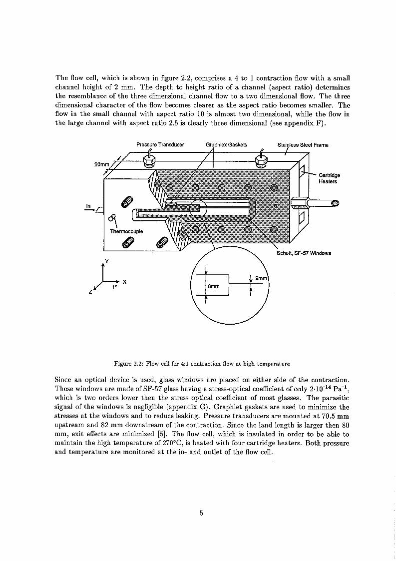
The flow cell, which is shown in figure 2.2, comprises a 4 to 1 contraction flow with a small channel height of 2 mm. The depth to height ratio of a channel (aspect ratio) determines the resemblance of the three dimensional channel flow to a two dimensional flow. The three dimensional character of the flow becomes clearer as the aspect ratio becomes smaller. The flow in the small channel with aspect ratio 10 is almost two dimensional, while the flow in the large channel with aspect ratio 2.5 is clearly three dimensional (see appendix F).

, SF-57 Windows

Figure 2.2: Flow cell for 4:l contraction flow at high temperature

Since an optical device is used, glass windows are placed on either side of the contraction. These windows are made of SF-57 glass having a stress-optical coefficient of only Pál, which is two orders lower then the stress optical coefficient of most glasses. The parasitic signal of the windows is negligible (appendix G). Graphlet gaskets are used to minimize the stresses at the windows and to reduce leaking. Pressure transducers are mounted at 70.5 mm upstream and 82 mm downstream of the contraction. Since the land length is larger then 80 mm, exit effects are minimized [5]. The flow cell, which is insulated in order t o be able to maintain the high temperature of 27OoC, is heated with four cartridge heaters. Both pressure and temperature are monitored at the in- and outlet of the flow cell.

5

Optical Rheometry

3.1 Flow Induced Birefringence

Light is an electro magnetic wave, characterized its electric field, since this fie has a stronger interaction with matter than the magnetic field. The time varying electric and magnetic fields are described by Maxwell’s equations. For non-conducting, non-charged media (as is the case in this setup), a light wave traveling in z-direction can be described as the superposition of two independent orthogonal components, see [i] and [7].

E = E,& + E,ZY0 with E, = E,o cos(& - k z ) E, = EY0 cos(wt - k z + S,,)

Here E.0 denotes the amplitude of the electric field in that direction, w the angular frequency, z the distance from the source, k the propagation number ( k = = :) and &, the relative phase difference between components.

3.1.1 Birefringence

The speed of iight depends on the eiectric ( E ) and magnetic (,u) properties of the medium in which it is propagating. The response of the material to the electric field of incident light is denoted by the index of refraction n. This index is defined as the ratio of the speed of light within the material (u) to this speed in vacuum (c = & -I): n = c/u. In anisotropic media, the binding forces between the atoms or molecules are not the same in the different directions. This can among others be caused by the geometrical shape of the molecules, as in polymers, or the distribution of electrons, as in ionogeneous materials. Therefore, the interactions with the magnetic field (and the refractive index also) differ with the directions. If there is one symmetry axis (called an optic axis) in the system, the medium displays two distinctive principal indices of refraction. Those indices correspond to the directions parallel (n// = ne, extraordinair) and perpendicular (ni = no, ordinair) to the optic axis. The birefringence of the medium is defined as An = n// - n1. When a light ray is propagating along the optic axis, it will only experience the ordinair refractive index, but in general it will experience both. One can think of the light ray as being composed of two separate rays: one with its electric field parallel to the optic axis and one perpendicular to it. It is possible that both rays propagate in different directions, due to the different refractive indices they

6

experience. If the (composed) light ray is incident on a surface which is perpendicular to the optical axis, both rays will travel the same way, but at different speeds:

E = EI/ë)/ + ElZ l with Ell = Ello cos(wt - zn1l.z) E l = El0 cos(wt - :n l z + &,)

E = Ello cos(wt + óx)Z’l + El0 cos(wt + ó,)ë‘l with 6, = - z n l / z 8, = - w . ~ ~ I z + 6, - ó, = ó,, + :Anz

The birefringence introduces an extra phase difference :&u, which shall be called the retar- dation 6 from this point forward.

3.1.2 Flow Induced Birefringence

In (polymeric) liquids which are not subject to any force fields, there is a random orientation of the molecules and therefore there is no birefringence. When these molecules are oriented by a velocity gradient, flow induced birefringence occurs. There are two forms of birefringence: intrinsic and form birefringence. Intrinsic birefringence is caused by the inherent anisotropy of the polarizabilities of the macromolecules making up the sample. For polymeric liquids the intrinsic birefringence can be explained by considering a macromolecule as a collection of segments, with each an anisotropic polarizability due to its anisotropic distribution of atoms. Orientation of the individual segments will then cause intrinsic birefringence. Form birefringence is due to a refractive index difference on a much larger scale. It occurs when the shape of the dissolved or suspended constituents is anisotropic and coupled with a difference in refractive index between the medium and the constituents. For concentrated polymer solutions and polymer melts, form birefringence is negligible [15].

3.1.3 Linear Stress Optical Rule

The basic idea of the stress optical rule, apart from the idea of optically anisotropic chain links, is that the interactions between polymer molecules are sufficiently localized and long-lived to treat them as junctions in a deforming network [15]. As in rubber elasticity, the orientation of these chain segments are considered to determine the state of stress. Since it does not, coxrttain any terms caused by direct internal friction, the stress can be correlated to orientational birefringence, which is assumed to be caused by the orientation of the optically anisotropic chain links (intrinsic birefringence). The linear rule between stress and birefringence is called the linear stress optical rule:

An = CAT (3.2)

Here A n denotes the deviatoric part of the refractive index tensor and Ar the deviatoric part of the Cauchy stress tensor. Both the principal refractive indices as the principal stresses are orientated at an angle x = xn = xT with the laboratory axes. The first laboratory axis is in the direction of the flow, the last is in the neutral direction (direction of the laser beam) and the second axis is perpendicular to both other axes (see figure 2.2). The principal refractive index difference Ani and the viscoelastic contribution to the ith principal stress difference 7i

of the polymeric liquid are related by the stress optical coefficient C, which is derived from the theory of freely rotating chain segments: C = 5 k T & F ( a 1 - a2), with k the Boltzmann constant, T the absolute temperature, N the number of segments, EO the dielectric constant

7

and Q the polarizability [i]. The stress optical coefficient used is 3.5 . lo-' Pa-', which is the mean of the values found in literature (varying between 2.5 . lo-' and 4.5 . lo-' Pa-'). Using this value, the absolute values for stress are assumed to be only accurate to within 15% [9]. Although the rubber elastic theory predicts unrealistic viscoelastic material functions, the linear relationship can be successfully applied in a wide range of experiments, even those of which the concentrations and deformation rates are outside the range for which the theory was developed [15]. According to Janeschitz-Kriegel [8] experience shows that in general the linear stress optical rule holds for polymeric melts. In flows of flexible chain polymer melts, the linear rule has been verified for shear stresses up to lo4 Pa and extensional stresses as high as lo6 Pa [5]. At high Deborah numbers, the stress optical rule is expected to break down, since the stress will continue to increase, whereas the orientation of the polymer chains is saturated. The rule will also fail when form birefringence is present [4], [15].

3.2 Pointwise Measurements

The optical setup for quantitative, pointwise measurement (see figure 3.1) consists of:

o a 10 mW red HeNe-laser (623.8 nm) as monochromatic light source

o a linear polarizer, mounted at O"

o an Electro Optic Modulator (EOM), which is a time dependent retarder with retardation At, mounted at 90"

o a quarter wave plate, mounted at O"

0 a focusing lens, f=90 mm, to reduce the waist of the laser beam along the optical path in the flow cell

0 the flow cell, which is a retarder with retardation 6 and orientation x 0 a quarter wave plate, mounted at 90"

o a linear polarizer, mounted at 90"

o a photodiode to detect the intensity of the beam

The EOM is controlled by an arbitrary waveform generator, which generates a saw-tooth signal. The fast response of the EOM makes it theoretically possible to use a signal frequency of 1 MHz, but the maximum frequency used in practice was 200 kHz, at which the fall time of the linear ramp is a sufficiently small percentage of one period [9]. The calibration of the optical devices is described in appendix B. The optical train is placed on two translation stages, controlled by a compumotor. The accuracy of this translation is 25.10-5 inch = 6,4 pm, which is less than the spatial resolution of the optical system, see appendix G. Using Mueller calculus (appendix A), the total intensity So of the light at the detector is given by:

10 . (1 - cos(2x) sin(6) sin(At) + s i n ( 2 ~ ) sin(S) cos(At)} 4

(3.3)

with x the orientation of the sample, 6 its retardation and At the retardation of the EOM. A lock-in amplifier is used to extract the in- and out-phase intensity:

10 1 0 sin - 4 zn - 4

I . - -I. - -- cos(2x) sin(6) IO IO 4 4

Ices = -IOut = - sin(&) sin(6)

8

(3.4)

O" 90" O" X 90" 90"

i source

EûIví QwP BOW ceii, S Q-WT LP

Figure 3.1: optical setup for pointwise measurements

The quantities li, and IOut can be calculated from the measured data by using the following equations:

Corr is a correction factor for the imperfectness of the optical system, see appendix B. I b g

denotes the signal if there is no light incident on the detector and IOC is the direct current intensity. Once li, and rout are known, the retardation S and the relative orientation x of the optical axis of the sample to the laboratory axis can be determined. When the stress optical rule applies, the first normal stress difference Ni (= axx - aYy) and the shear stress T~~ can also be calculated. It is assumed that 1x1 < i.14, so that cos(2x) is always positive.

s = -sign(Ii,) . arcsin 4- (3.6) 1 Iout

2 Iin x = -- arctan(-)

6 cos (2x) A0

2ndC Ni = ~ (3.7)

C is the stress optical coefficient(3.5 . lo-' Pa-'), d the depth of the flow cell (20 mm) and A0 the wavelength of the used light (623.8 nm).

3.3 Fieldwise Measurements

The advantage of fieldwise measurements is the capability to visualize the entire stress field, in both steady and transient flows. The birefringence can be made visible with isoclinic lines and isochromatic lines. The setup for measurement of isoclinic lines is shown in figure 3.2.

source i- flow cell, 6 k LP camera

Figure 3.2: optical setup for isochromatic and isoclinic lines

9

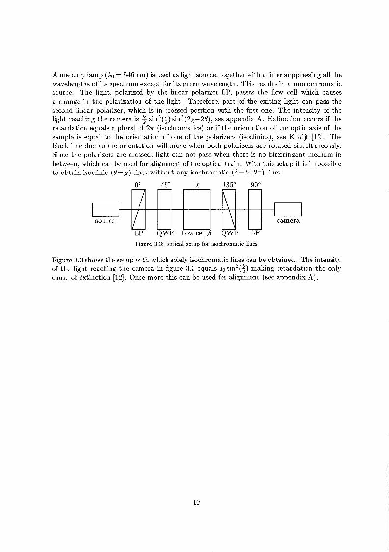
A mercury lamp (A0 = 546 nm) is used as light source, together with a filter suppressing all the wavelengths of its spectrum except for its green wavelength. This results in a monochromatic source. The light, polarized by the linear polarizer LP, passes the flow cell which causes a change in the polarization of the light. Therefore, part of the exiting light can pass the second linear polarizer, which is in crossed position with the first one. The intensity of the light reaching the camera is 4 sin2 ($1 sin2 (2x-269, see appedin A. Extinction occurs if the retardation equais a piurai of 27r (isochromaticsj or if the orientation of the optic axis of the sample is equal to the orientation of one of the polarizers (isoclinics), see Kruijt [12]. The black line due to the orientation will move when both polarizers are rotated simultaneously. Since the polarizers are crossed, light can not pass when there is no birefringent medium in between, which can be used for alignment of the optical train. With this setup i t is impossible to obtain isoclinic (û=x) lines without any isochromatic (S=k an) lines.

O" 45" X 135" 90" - -

- - source

Figure 3.3: optical setup for isochromatic lines

camera

Figure 3.3 shows the setup with which solely isochromatic lines can be obtained. The intensity of the light reaching the camera in figure 3.3 equals 1osin2($) making retardation the only cause of extinction [12]. Once more this can be used for alignment (see appendix A).

10

Data Acquisition

Optical rheometry is used to acquire local and full field stress information in a polymer flow. Hereby both transient and steady flow are important. To get quantitative data over a line or a field with the pointwise measurement method, it is necessary to have steady flow. The fieldwise method can be used for both steady and transient flows , which is useful for determining the number of order transitions (see appendix C). This chapter treats the data acquisition of these methods, as well as some errors.

4.1 Pointwise Measurements: Steady Flow

In steady flow, data can be measured in more then one point by using a compumotor. Both lines and areas can be scanned, but line scans proved to give more information in relation to the occupied time. The compumotor needs information about the begin and end position, the number of steps in between and the delay time (6 sec) the data logger needs to read and store information. It controls two XY tables simultaneously: one XY table supports the optical components on one side of the flow cell, the other the components on the opposite site. In this way, the alignment of the optical train can be remained, while the position of the laser beam in the flow cell changes. Once the intensity of the laser beam is detected, a signal is transfered to the lock-in amplifier and the current stream detector. The lock-in amplifier electronically filters the signal and transfers the factors Isin and IC,,, respectively belonging to the terms sin(At) and cos(At), see equation 3.4. A data logger and an in-house written control program for a leading personal computer are used to acquire the data, which is stored in ASCII files, containing successively:

x y time data I,in I,,, IOC PI P2 - Ti T2

The position of the laser beam is stored in x and y, and the intensities in IOC, Isin and I,,,. Pi and P2 denote respectively the inlet pressure and outlet pressure of the flow cell. The next position is not used and Ti and T2 are the inlet temperature and outlet temperature of the polymer melt. This data is preceded by the information used by the compumotor.

11

Function Generator

U Function

Q1 Generator

- - - - -

polymer

Q2 -$ P2

L: P1 ,P2: EOM: Q1 ,Q2: FC:

laser polarizes electro-optic modulator quarter-wave plates flow-cell detector amplifier lock-in amplifier low-pass filter

5??& Intensit Si nai

I ( t ) = ${l + sin(At) sin(6) - cos(2x) - cos(At) - cos(6) - s in (2~) )

Figure 4.1: Rheo optical analyzer for flow birefringence measurements

4.2 Processing of ASCII Files

After the format of the ASCII files has been adjusted, they are processed with the in-house written program dataproc.m (see appendix I), which is implemented in the calculation program Matlab. The following commands are programmed:

o read ASCII file

o get correction factor

o calculate I;, and IOUt using equation 3.5.

e plot I;, and IoUt against the position and ask wheLer the -Tiin signa! has to be modified. This is necessary when the optics are not good aligned, see section 4.4.

o get background intensity for li, and lout and calculate the adjusted I;, and lout if necessary.

o calculate x and 6 using equation 3.6.

o if necessary, modify S for order transitions (see appendix C):

- get the positions of the points that have to be modified

- get the modification factor (a plural of T)

- ask whether the calculated 6 should be added to or subtracted from this factor

- calculate the new S - ask whether there are other points that need modification, and if so, repeat.

o calculate rzy and Ni using equation 3.7.

12

o calculate the mean temperature and pressure difference and their standard deviations.

o save all the calculated and original information.

The calculated quantities are written to file which can be used to make graphics.

The first black lines to be identified, are the isoclinic lines. These lines move if the polarizers are rotated simultaneously. Their interpretation is simple: at every point covered by the isoclinic line, the orientation of the principal refractive indices (and therefore of the principal stresses) is at either an angle 9 or an angle O + with the laboratory axes. Once the isoclinic lines and the isochromatic lines are identified, the retardation can be determined. For a quantitative measurement of the retardation, the accuracy of the fieldwise method is low, caused by the broadness of the black lines. The measurements are useful as a qualitative view of the total field and as a rough estimate of the retardation in transient flows. Using a mercury lamp, extinction occurs when the optical path difference A = dan equals a plural of 546 nm, the wavelength A. Each of these black lines therefore corresponds to a retardation S which equals a plural of 27r. Since the wavelength of the mercury lamp is smaller than the wavelength of the HeNe laser, the order transitions occur at different positions, so that the photographs can be used to check the data measured by the pointwise method. Each black line corresponds to an equivalent stress level of 7800 Pa (& . (27r) = s.1~~$?~~o-9 Pa). The

equivalent stress is defined as d m . 4.4 Errors

Errors can among others be caused by the angles of the optic elements, which cause other terms of S and x in both I s in and I,,,. When scanning an intersection, this error becomes clear, because the signal is not symmetric in regard to the centerline anymore. For the terms which are both part of Isin and I,,,, the data can be corrected by subtracting a constant times I,,, from Is in and visa versa, but I,,, also contains some terms which are not in Is in .

These terms influence the calculated S and x. Another source of errors is the noise on the signal. When Isin is almost zero, the noise can cause S to change sign. The sign of the angle x is influenced by noise on both Isin as Icos and if both Isin as IC,,, are almost zero, the magnitude of x can also be greatly influenced by the noise. Temperature gradients can also cause errors, since they cause the laser beam to follow a curved path. By adjusting the temperature manually, these errors were prevented.

13

Results

in

Y

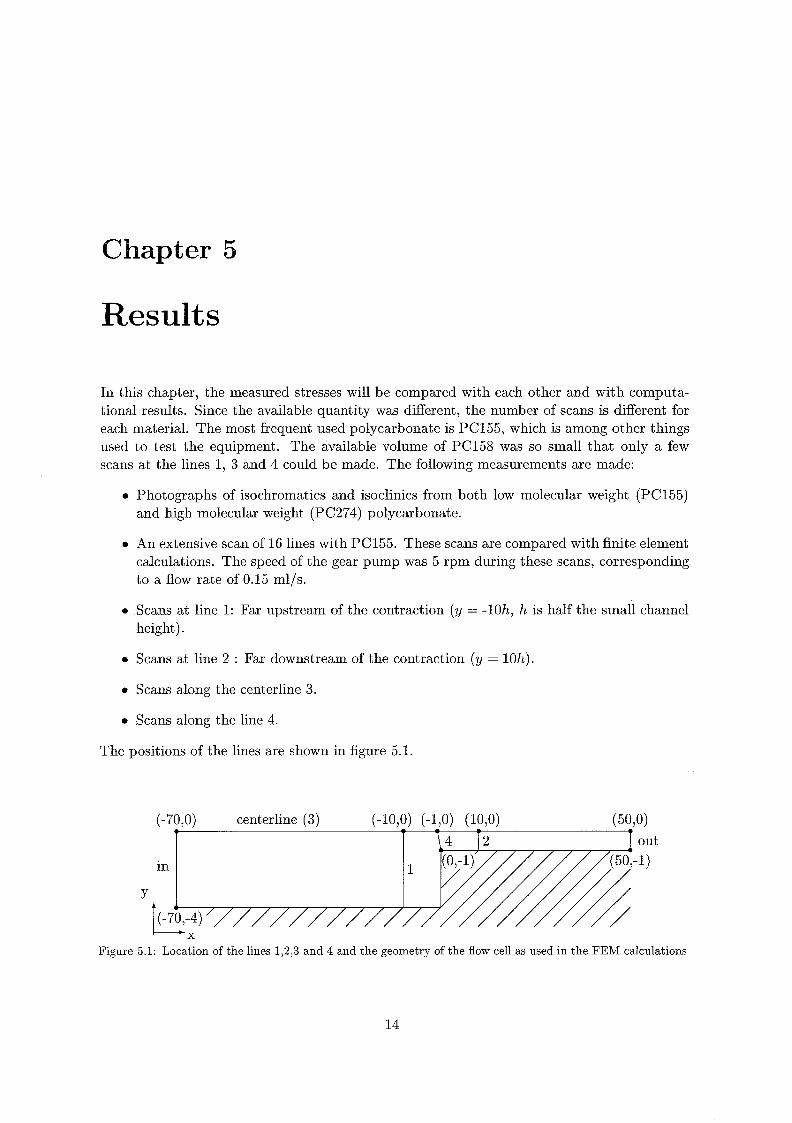
In this chapter, the measured stresses will be compared with each other and with computa- tional results. Since the available quantity was different, the number of scans is different for each material. The most frequent used polycarbonate is PC155, which is among other things used to test the equipment. The available volume of PC158 was so small that only a few scans at the lines 1, 3 and 4 could be made. The following measurements are made:

o Photographs of isochromatics and isoclinics from both low molecular weight (PC155) and high molecular weight (PC274) polycarbonate.

out

1

o An extensive scan of 16 lines with PC155. These scans are compared with finite element calculations. The speed of the gear pump was 5 rpm during these scans, corresponding to a flow rate of 0.15 ml/s.

o Scans at line 1: Far upstream of the contraction (y = -10h, h is half the small channel height).

o Scans at line 2 : Far downstream of the contraction (y = 10h).

o Scans along the centerline 3.

o Scans along the line 4.

The positions of the lines are shown in figure 5.1.

14

5.1 Numerical Met hod

mode 1 2 3 4

0.1 1 o' I o3 I os

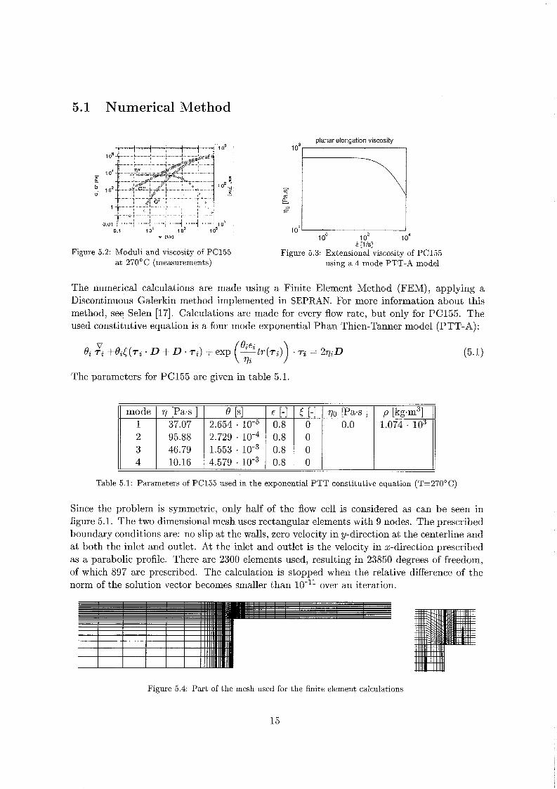
7 [Pa.s ] Q [SI E [-I t [-I 7 0 [Pa.s 1 P [kg.m31 37.07 2.654 . 0.8 O 0.0 1.074 . lo3 95.88 2.729 . 0.8 O 46.79 1.553 . 0.8 O 10.16 4.579 . 0.8 O

planar elongation viscosity

w [llr] 1 oo 1 o' i o4 I [Ik]

Figure 5.3: Extensional viscosity of PC155 using a 4 mode PTT-A model

Figure 5.2: ModuIi and viscosity of PC155 at 270°C (measurements)

The numerical calculations are made using a Finite Element Method (FEM), applying a Discontinuous Galerkin method implemented in SEPRAN. For more information about this method, see Selen [17]. Calculations are made for every flow rate, but only for PC155. The used constitutive equation is a four mode exponential Phan Thien-Tanner model (PTT-A):

( y ) 27iD (5.1) v

Qi ~i + 1 3 i [ ( ~ i . D + D . ~ i ) + exp - h - ( ~ i ) . ~i =

The parameters for PC155 are given in table 5.1.

Since the problem is symmetric, only half of the flow cell is considered as can be seen in figure 5.1. The two dimensional mesh uses rectangular elements with 9 nodes. The prescribed boundary conditions are: no slip at the walls, zero velocity in y-direction at the centerline and at both the inlet and outlet. At the inlet and outlet is the velocity in rc-direction prescribed as a parabolic profile. There are 2300 elements used, resulting in 23850 degrees of freedom, of which 897 are prescribed. The calculation is stopped when the relative difference of the norm of the solution vector becomes smaller than lo-'' over an iteration.

Figure 5.4: Part of the mesh used for the finite element calculations

15

5.2 Fieldwise Method

In figure 5.5 isochromatics are shown for PC274 at the lowest speed (upper part of the figure) and for PC155 at the highest speed (lower part). Every black line represents a stress difference of 7.8 kPa (see section 4.3). The maximum stress obtained at the centerline with PC155 is about 9 kPa. The stress obtained with PC274 at 0.15 ml/s is higher (about 10 kPa), but qualitatively the two photographs iook alike. The isuclinics, which indicate the places where the orientation angle x is 45", are shown in figure 5.6 for PC274 at a speed of 0.15 ml/s. This 'bug'-like picture is characteristic for the 45"-isoclinics at both material/speed combinations. The vertical black lines are isochromatics, identical to those in the upper half of figure 5.5. The advantage of the fieldwise method becomes clear in figure 5.7, since pointwise measurements are of no use here except for the scan along the centerline. Downstream of the contraction, for example, one should correct for about 15 order transitions, which is approximately one order transition for every three data points. Taking measurement errors into account, this is almost impossible to do. For the centerline one encounters 'only' five order transitions until the maximum stress (three fringes x 24 kPa) is reached. Therefore, this pointwise scan can still be used along the centerline as is shown in figure 5.23. Furthermore, the fieldwise method is suitable to determine which points or lines are of interest. As can be seen from figure 5.7, stresses are highest at the corner and therefore a scan is made from the centerline to the corner at an angle of 45"with the 2-direction. A good view of the extensional stresses can be obtained at the centerline. As figures 5.5 and 5.7 show, the flow becomes fully developed again at about a distance h behind the contraction (isochromatics are parallel again), more or less independent of the flow rate. The influence of the contraction on the flow upstream does depend on the flow rate: the higher the flow rate, the larger the influence of the contraction. Since the influence of the contraction seems already negligible at a distance of three times the small channel height (6h) at the highest flow rate, scans at a distance of 10h from the contraction are expected to show fully developed flow.

Figure 5.5: Isochromatics: PC274 a t 0.15 ml/s (upper part) and PC155 at 0.88 ml/s (lower part), The maximum stress at the centerline is about 10 kPa

Figure 5.6: Isochromatics + isoclinks: PC274 at 0.15 ml/s. The isoclinics correspond to an orientation angle of 45'

16

Figure 5.7: Isochromatics: PC274 at 0.44 ml/s, maximum elongational stress at centerline about 24 kPa

5.3 Total Scan

Figure 5.8: PC155: c ~ ~ ~ - c ~ ~ ~ , 0.15 ml/s - = numerical , x = experimental

Figure 5.9: PC155: Í - ~ ~ , 0.15 ml/s - = numerical , x = experimental

With PC155, an extensive scan has been performed at a flow rate of 0.15 ml/s. Scans were made at respectively x = -10h, -2h, -h, -0.5h, O, 0.25h, 0.5h, h and 10h, with h = 1 mm (half the small channel height). The first normal stress differences and shear stresses were derived from the measurements and compared with FEM results. In figures 5.8 and 5.9 the numerical results are represented with solid lines (top half), the experimental values with crosses (bottom half). The deviation for NI near the wall is quite large at some cross-sections downstream of the contraction. This will be discussed in more detail in appendix D. However, the overall

17

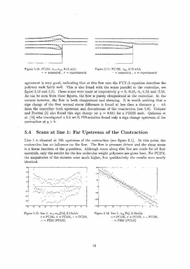
Figure 5.10: PC155: mzz-myy, 0.15 ml/s Figure 5.11: PC155: 0.15 ml/s - = numerical , x = experimental - = numerical , x = experimental

agreement is very good, indicating that at this flow rate the PTT-A equation describes the polymer melt fairly well. This is also found with the scans parallel to the centerline, see figure 5.10 and 5.11. Those scans were made at respectively y = 0,-0.5h,-h,-1.5h and -2.5h. As can be seen from these figures, the flow is purely elongational at the centerline. At the corners however, the flow is both elongational and shearing. It is worth noticing that a sign change of the first normal stress difference is found at less then a distance y = *h from the centerline both upstream and downstream of the contraction (see 5.8). Galante and Frattini [5] also found this sign change (at y = 0.8h) for a PDMS melt. Quinzani et al. [16] who investigated a 5.0 wt.% PIB-solution found only a sign change upstream of the contraction at y > h.

5.4 Scans at line 1: Far Upstream of the Contraction

Line 1 is situated at 10h upstream of the contraction (see figure 5.1). At this point, the contraction has no influence on the flow. The flow is pressure driven and the shear stress is a linear function of the y-position. Although scans along this line are made for all four materials, only the results for the low molecular weight polymers are given here. For PC274, the magnitudes of the stresses were much higher, but qualitatively the results were nearly identical.

80

- L .

60

Figure 5.12: line 1: c ~ ~ ~ - c ~ ~ ~ [ P a ] , 0.15ml/s o = PC145, x = PC155, + = PC158, - = FEM (PC155)

o 1 2 3 -1501

Figure 5.13: line 1: pal, 0.15ml/s

-4 -3 -2 -1

O = PC145, x = PC155, + = PC158, - = FEM (PC155)

18

Normal stress differences are shown for the materials PC145(0), PC155(x) and PC158(+) at a flow rate of 0.15 ml/s in figure 5.12 and at a flow rate of 0.44 ml/s in figure 5.14. The solid line indicates the FEM results for PC155. The same symbols are used in figure 5.13 and 5.15, in which the shear stress is shown for a flow rate of 0.15 and 0.44 ml/s respectively. For

.. * ._ -60 - .

I . . - * - _ Ij-

-80 ? , , S S

- 5 - 4 - 3 - 2 - 1 o 1 2 3 4 5

500

2 3 -5001

-4 -3 -2 -1 o 1

Figure 5.14: Line 1: ~ ~ ~ - o ~ ~ [ P a ] , 0.44 ml/s Figure 5.15: Line 1: pal, 0.44 ml/s O = PC145, x = PC155, + = PC158, 0 = PC145, x = PC155, + = PC158, - = FEM (PC155) - = FEM (PC155)

both flow rates, the experimental shear stress data agrees with the numerical data, whereas the data for the first normal stress difference does not. Since the magnitude of Ni calculated with the experimental data is equal for both flow rates, the difference will rather be caused by measurements errors than by a numerical error. In theory, the order of magnitude is described by:

- cvdi c vi with X = -

For PC155, this gives 1 = 7.706.10-4s. The shear rate at the large channel wall is E s-' and s-l, giving first normal stress differences of 0.148 Pa and 1.27 Pa at the flow rates 0.15 and 0.44 ml/s respectively. The resemblance with the numerical results (0.15 Pa and 1.30 Pa) makes clear that the difference is indeed caused by inaccurate experimental data. It can not, however, be caused by noise, since a (shifted) parabolic profile is shown for every material. The resemblance between the data of the different scans concerning the orientation and retardation are shown in figures 5.16 and 5.17.

Figure 5.16: Line 1: Orientation x, 0.15 ml/s o = PC145, x = PC155, + = PC158, - = FEM (PC155)

Figure 5.17: Line 1: Retardation 6, 0.15 ml/s O = PC145, x = PC155, + = PC158, - = FEM (PC155)

19

5.5 Scans at line 2: Far Downstream of the Contraction

Line 2 is positioned at 10h downstream of the contraction. Because of the small amount of PC158, this scan is only made for the materials PC145(0) and PC155( x). As with the scans at line 1, the experimental and numerical data of the shear stress show little difference, except for some points very close to the wall, where the influence of the finite dimension of the laser beam becomes apparent (see appendix G for details). Estimating the order of magnitude of the first normal stress diiference shows that the numerical results are correct. A comparison with the results of the fieldwise method is made in appendix G. In contradiction to the

Figure 5.18: Line 2: oZz-oyy[Pa], 0.15 ml/s Figure 5.19: Line 2: ~-,~[Pai], 0.15 ml/s o = PC145, x = PC155, o = PC145, x = PC155, - = FEM (PC155) - FEM (PC155)

results found at line 1, the first normal stress difference found here resembles the numerical data in the middle of the channel (no large shift). The same resemblance is found when regarding the orientation and retardation (see appendix D). Towards the walls however, a large deviation is found in the orientation x, causing the deviation in Nl. The magnitude of those errors is discussed in more detail in appendix D. The cause of the deviation in x could not be determined, but possible causes include reflections of the laser beam on the wall, which interact with the signal and thermal effects caused by high shear rates (viscous heating).

5.5 Scans at h e 3: Centerline

Figure 5.20, 5.21 and 5.22 show the first normal stress difference (in Pa) at the flow rates 0.15, 0.44 and 0.88 ml/s, corresponding to a wall shear rate downstream of the contraction of 11, 33 and 67 s-l respectively.

6000

I I o 2 6 -8 -5 -4 -2 o 4 6

-,ow -200 -8 -6 4 -2

Figure 5.20: Line 3: ozz-oyy[Pa], 0.15 ml/s Figure 5.21: Line 3: o,,-ayy[Pa], 0.44 ml/s o = PC145, x = PC155, + = PC158, - = FEM (PC155)

O = PC145, x = PC155, + = PC158, - = FEM (PC155)

20

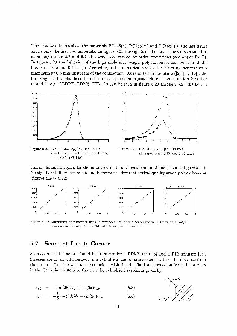
The first two figures show the materials Pc145(0), PC155(x) and PC158(+), the last figure shows only the first two materials. In figure 5.21 through 5.23 the data shows discontinuities at among others 2.2 and 6.7 kPa which are caused by order transitions (see appendix C). In figure 5.23 the behavior of the high molecular weight polycarbonate can be seen at the flow rates 0.15 and 0.44 ml/s. According to the numerical results, the birefringence reaches a maximum at 0.5 rnm upstream ofthe contraction. As reported in literature ([2], [ 5 ] , [is]), the birefringence has also been found to reach a maximum just before the contraction for other materials e.g. LLDPE, PDMS, PIB. As can be seen in figure 5.20 through 5.23 the flow is

2 -

.. .. . . 1

i 1 5

i -

’i I I

.. , , , ” , , ,

-6 -5 -4 -3 -2 -1 o 1 2 3 4

Figure 5.22: Line 3: rzz-oYy[Pa], 0.88 ml/s Figure 5.23: Line 3: o,,-oyy[Pa], PC274 O = PC145, x = PC155, + = PC158, at respectively 0.15 and 0.44 ml/s - = FEM (PC155)

still in the linear region for the measured material/speed combinations (see also figure 5.24). No significant difference was found between the different optical quality grade polycarbonates (figures 5.20 - 5.22).

10000 _:;__I_i 1 ; y

4000

2000

O O 033 0.67 1 O 0.33 0.67

1 o m

4000

2000 ::E O 0.33 0.67

_I_/ 2

1

0- O 0.33 0.67

Figure 5.24: Maximum first normal stress differences [Pa] at the centerline versus flow rate [ml/s] 0 = measurements, + = FEM calculation, - = linear fit

5.7 Scans at line 4: Corner

Scans along this line are found in literature for a PDMS melt [5] and a PIB solution [16]. Stresses are given with respect to a cylindrical coordinate system, with T the distance from the corner. The line with 8 = O coincides with line 4. The transformation from the stresses in the Cartesian system to those in the cylindrical system is given by:

21

0-

-200

-4w

-6W

-800

-1000-

-1200-

-1400 ! I

-

-

-

-

I 0 5 1 1 5

-1600'

Figure 5.25: Line 4: C T ~ ~ - C T ~ B B [ P ~ ] , 0.15 ml/s o = PC145, x = PC155, + = PC158, - = FEM (PC155)

#i+&;; " :;<+oo .f o

* " O + i o o ol +?'X 0 5

..' o i X

-.-i: O . "M

O 0.5 -8"-

1

Figure 5.26: Line 4: r ,~[Pa], 0.15 ml/s o = PC145, x = PC155, + = PC158, - FEM (PC155)

In figure 5.25 the first normal stress difference nrr-ao~ is shown for the low molecular poly- carbonates, which corresponds to 2rzv in the Cartesian coordinate system. Figure 5.26 shows rro corresponding to -2(ozz-nyy). The shear stress rro shows a good agreement with the numerical results, but the normal stress difference orr - OgQ found experimentally is smaller than its numerical value when approaching the corner. This was also found by Galante and Frattini [5] for PDMS melts. They suggested that the lower normal stress difference was caused by corner rounding, since this decreases the change in velocity undergone by fluid elements passing near the corner. Since (orr - oog) seems to approach a constant value as T + O and Newtonian analysis predicts that Ni - TO.' [16], another explanation could be that the numerical results calculated with the Phan Thien-Tanner A model are incorrect near the corner. Although there is a significant difference found at this line between the numerical and experimental results, there was no difference found between the optical quality grade polycarbonates.

1

22

Conclusions

The purpose of this work was to look for differences between the flow behavior of three opti- cal grade polycarbonates. Moreover, a correlation between the experiments and the injection moulding process of compact discs was desirable. The behavior of the polycarbonates is stud- ied in a 4 to 1 contraction, using both a pointwise and a fieldwise Flow Induced Birefringence (FIB) technique. This report shows that it is very well possible to obtain detailed stress data at 270"Celsius using a Flow Induced Birefringence technique based on phase modulation. The spatial resolution obtained with the system was in the order of 100 pm.

Under the present conditions, no significant differences were found between the different OQ-grade polycarbonates. No qualitative differences were found between the low and the high molecular weight polycarbonates either. Differences might be found at higher shear and elongational rates, when the linear region is abandoned. The numerical simulations performed using a PTT-A model show little difference with the measurements of the OQ- grade materials upstream of the channel. Downstream of the channel deviations in the first normal stress difference are found near the wall. Further investigation will be necessary in order to find an explanation.

Although no differences were found between the two-dimensional numerical simulations and the measurements, one should notice that the flow in the large channel is three dimensional It is difficult to give direct physical interpretation of the apparent birefringence and extinction angle when these properties vary along the optical path [5].

In order to discover any differences between the three optical quality grade polycarbonates, more measurements are necessary. These should be made at higher flow rates, for which the flow cell should be adjusted. The flow cell should have a height to depth ratio of 10 for the large channel, in order to get a two dimensional flow. Higher shear and elongational rates can be achieved by reducing the channel height, but one should take into account that this also reduces the relative spatial resolution. Furthermore, higher flow rates automatically result in higher stresses, which might cause problems with the number of order transitions when using the pointwise FIB technique.

23

[l] J.P.W. Baaijens, Evaluation of Constitutive Equations for Polymer Melts and Solutions in Complex Flows, Ph.D.thesis, Eindhoven University of Technology, Eindhoven 1994.

[2] P. Beaufils, B. Vergnes and J.F. Agassant, Characterization of the Sharkskin Defect and its Development with the Flow Conditions, in: International Polymer Processing, vol IV, issue 1, Munich 1989.

[3] E. Collett, Polarized Light, fundamentals and applications, Marcel Dekker, New York, 1993, p 33-90.

[4] G.G. Fuller, Optical Rheometry, Annual Review of Fluid Mechanics, vol 22(1990), p 387-417.

[5] S.R. Galante and P.L. Frattini, Spatially Resolved Birefringence Studies of Planar Entry Flow, Journal of Non-Newtonian Fluid Mechanics, vol 47( 1993), p 289-387.

[6] S.R. Galante and P.L. Frattini, A n Inviscid Approximation for the Centerline Deformation History in Entry Flows, AIChE journal, Vol. 39(1993), no 5.

[7] E. Hecht, Optics, Addinson-Wesley Publishing Company, Inc, Reading, 1987.

[8] H. Janeschitz-Kriegel, Polymer Melt Rheology and Flow Birefringence Springer-Verlag, Berlin/Heidelberg, 1983.

191 T. Jordan, intern report, GE R&D, Schenectady, 1995.

[lo] R.M. Kannan and J.A. Kornfield Stress-optical manifestations of molecular and microstructural dynamics in complex polymer melts, Journal of Rheology, 38(4) July/August 1994.

24

[li] P.G.M. Kruijt, The Rheo-Optical Analyzer for Birefringence Measurements, WFW 94.011, Eindhoven University of Technology, Eindhoven, 1994.

[12] P.G.M. Kruijt, Experimental and Numerical Analysis of Polymer Melt Flow Past a Constrained Cylinder, WFW 94.133, Ei~dh~ve:: Ur,iïersity ef Sechr.o!egy, Y i n d h ~ ~ e n , 1994.

[13] G.H. McKinley, Nonlinear Dynamics of Viscoelastic Flows in Complex Geometries, Massachusetts Institute of Technology, Massachusetts June 1991, p 296-304.

[14] T. Nagai, Y. Kimizuka, K. Nito, and J. Seto, Melt Viscosity and Flow Birefringence of Polycarbonate, Journal of Applied Polymer Science, vol 44(1992), p 1171-1177.

[15] L.M.Quinzani, Birefringence Studies of Entry Flows of Concentrated Polymer Solutions, Massachusetts Institute of Technology, Massachusetts 1991, p 81-89.

[16] L.M. Quinzani, R.D. Armstrong and R.A. Brown, Birefringence and laser-Doppler velocimetry (LDV) studies of viscoelastic flow through a planar contraction, Journal of Non-Newtonian Fluid Mechanics, vol 52(1994), p 1-36.

[17] J.H.A. Selen, Multi-mode viscoelastic computations of complex flows, WFW 95.141, Eindhoven University of Technology, Eindhoven, 1995.

25

Mueller Calculus

Mueller calculus can be used to describe polarized, partly polarized and unpolarized light. It has the advantage, that one can measure its four parameters directly. Those four parameters are (using equation 3.1) [3], [li]:

so = E,, 2 + E;, = total intensity SI = E;, - Ey, = linear horizontal of vertical polarization s2 = 2E,oE,o cos 6 = linear +45"or -45"polarization S3 = 2E,oE,o sin6 = right or left circular polarization

For any polarization state Si 2 Sl + ,522 + S:, whereas the equality sign applies for completely polarized light. The interaction of light with matter can be described by Mueller matrices. Therefore, the four parameters are written in a column matrix S = [SO SI S2 &,IT. For every optical device there exists a Mueller matrix M such that the emerging beam, indicated as S', can be calculated by S' = M . S. The Mueller matrices for a retarder lrm and a polarizer lpm are:

r 1 O O o 1 Ideal Linear Retardation Matrix lrm (a) =

Ideal Linear Polarization Matrix lpm =

O 1 O O O COS@ s ina O O -sina! cosa

O O

1/2 1/2 o 1 /2 1/2 o

l o O O O O O

Above matrices denote retarders and polarizers with the orientation parallel to the laboratory axes. When they are rotated over an angle O in respect to those laboratory axes, they are described by

Lrm (0,a) = rot (O) lrrn (a) rot ( - O ) Lpm (O) = rot (O) lpm rot (-0)

With Rotation Matrix rot ( O ) =

1

1 O O O cos20 sin20 O -sin20 cos20 O O O O

27

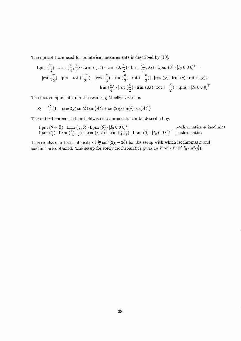
The optical train used for pointwise measurements is described by [lo]: 7r 7 r 7 T 7r 7T

Lpm (-) . Lrm (-, -) . Lrm (x, 6) . Lrm (O, -) . Lrm (-,At) . Lpm (O) . [Io O O 0IT = 2 4 2 2 4 7T -IT 7T 7r 7T r,,+ í 1 . 1,- 1-11 . rrnt I-\ .i,- (-\ . rnt [--)I . rrnt (-,\ -i,-- 1x1 . rr\t (-..\I .

lrm (-) . [rot (-) . lrm (At) . rot (- -)] . Ipm . [Io O O 0IT

I"' \ h J J LLUIJ (5) iyui - IUIJ \ - LIUU i 2 ) 11111 \ J I W U \ / J L 1 W U \A, 11111

Ir 7T 7r

4 2 2

The first component from the resulting Mueller vector is

1 0

4 So = -{i - cos(2x) sin(6) sin(At) + sin(2x) sin(6) cos(&)}

The optical trains used for fieldwise measurements can be described by:

Lpm (6' + Fj) . Lrm (x, ó) . Lpm (6') . [IO O O 0IT Lpm (5) . Lrm (%, ;) . Lrm (x, 6) . Lrm (i, 5) . Lpm (O) . [IO O O O]*

isochromatics + isoclinics isochromatics

This results in a total intensity of 9 sin2(2x - 26') for the setup with which isochromatic and isoclinic are obtained. The setup for solely isochromatics gives an intensity of Io sin2($).

28

Annendix B - -rr -----*-

Calibrat ion Optical System

The Mueller representation of the optical system for pointwise measurements is 7r 7 r 7 r 7r 7r

Lpm (-) . Lrm (-, -) . Lrm (x, S) . Lrm (O, -) . Lrm (-, At) . Lpm (O) . [Io O O 0IT 2 4 2 2 4

Here Lpm (6) is a linear polarization matrix for a polarizer at an angle 6 with the 2-direction and Lrm (6, A) is a linear retardation matrix for a retarder with retardation h at an angle 13. The electro-optic modulator Lrm (2 , At) is fixed at 45" with respect to the first polarizer. The angle of this first polarizer is taken O". The calibration consists of successively adjusting the angles of the second polarizer, the second quarter wave plate and the first quarter wave plate. Finally the correction factor is determined. This calibration method is described in more detail by Kannan and Kornfield [lo].

B. 1 Second Polarizer

In order to determine the angle offset at which the second polarizer is at 90" with respect to the first polarizer, only the two polarizers and the EOM are used in the optical train. When the angle of the second polarizer is taken 4, the total intensity of the light reaching the detector is

IO 4 4

[i O O O ] . Lpm (4) . Lrm ( E , ~ t ) . Lpm ( O ) . [lo O O OIT = - {i + c o s ( ~ t ) cos(24)).

Since 4 should be go", the angle of the polarizer has to be adjusted until the out-phase component is minimal.

B.2 Quarter Wave Plates

When the second polarizer is fixed in the right position, the second quarter wave plate is inserted in the optical train at angle 8. The total intensity becomes

!? (1 - cos(At) c0s2(26) + sin(At) sin(28)). 4

29

The angle of the second quarter wave plate will therefore be at 45" when the in-phase component is maximal and the absolute value of the out-phase component is minimal. When the first quarter wave plate is also inserted, the intensity becomes % when this plate is at O". To obtain this, the angles of both the quarter wave plates should be adjusted until both the in- and out-phase components are zero.

Once all the optical elements are in the right position, the correction factor con is determined. Therefore, a third linear polarizer is inserted in the optical train, at the place where the flow cell should be. By rotating this polarizer, eight angles (45" apart) are found where either the in- or out-phase component is zero. For all these angles, the values of the in- or out-phase component unequal to zero (Iphase) and the direct current (IDc) are recorded. For all these pairs the quantity IPphase/(I~c -&g) is calculated, where Ibs denotes the background intensity, obtained when the laser is turned off. The correction factor is the mean of the absolute values of these eight divided by 0.714. This factor 0.714 (= ia) is caused by the amplifier, which returns the root mean square value.

30

Order Transit ions

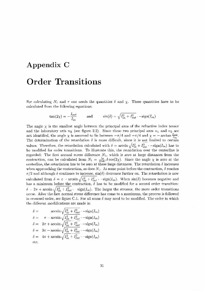
For calculating NI and T one needs the quantities 6 and x. These quantities have to be calculated from the following equations:

t a n ( 2 ~ ) = -~ Iout and sin(6) = d m . -sign(Ii,) 127%

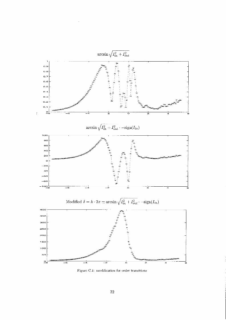
The angle x is the smallest angle between the principal axes of the refractive index tensor and the laboratory axis nx (see figure 2.2). Since these two principal axes n1 and 722 are not identified, the angle x is assumed to lie between -n/4 and +n/4 and x = - arctan e. The determination of the retardation 6 is more difficult, since it is not limited to certain values. Therefore, the retardation calculated with 6 = arcsin Jzn' I +Iout . -sign(Ii,) has to be modified for order transitions. To illustrate this, the retardation over the centerline is regarded: The first normal stress difference N I , which is zero at large distances from the contraction, can be calculated from NI = &6cos(2x). Since the angle x is zero at the centerline, the retardation has to be zero at these large distances. The retardation 6 increases when approaching the contraction, as does NI . At some point before the contraction, 6 reaches 7r/2 and although 6 continues to increase, sin(6) decreases further on. The retardation is now calculated from 6 = 7r - arcsin li, + lout . -sign(&,). When sin(6) becomes negative and has a minimum before the contraction, 6 has to be modified for a second order transition: 6 = 2n + arcsin d w . -sign(Izn). The larger the stresses, the more order transitions occur. After the first normal stress difference has come to a maximum, the process is followed in reversed order, see figure C.1. For all scans 6 may need to be modified. The order in which the different modifications are made is:

$""

6 = arcsin l / ~ & + I& . -sign(Ii,)

6 = n - arcsin .,/I:, + iout . -sign(ii,)

Y

etc.

31

1

0.9

O 8

07

O 6

o 5

o 4

o 3

0.2

o1

O -8 -6 -4 -2 O 2 4 6

arcsin d ~ : ~ + . -sign(ii,>

1 0 0 ,

-60 i:r x x x x

x x

x x -%O szc

-6 -4 -2 O 2 4 1 6 - 1 0 0

-8

Modified S = k ~ 27r zt aïcsia d m . -sip(Itn)

x x

x x

x ss

x

x x x

x x

x x x

x x x

Figure C.l: modification for order transitions

32

Error Analysis

As mentioned before in chapter 5, a difference is found at some cross-sections between numer- ical and experimental data of the first normal stress difference. In order to be able t o explain this difference in NI, the numerical values for x, 6 , I;, and lout are also calculated, using: x = -Zarctan( 1 & Ni )

I;, = - cos(2x) sin(S)

6 = Txy

lout = sin (2x) sin (S) A0 sin(2x)

The retardation S is linear dependent on the birefringence n1 - 122, where n1 the refractive index in the direction under an angle x with the laboratory x-axis. When x is taken as the angle between the other (perpendicular) axis 122 and the x-axis (1x1 > n/4), the birefringence is calculated as n2 - nl. At some cross-sections x and S are simultaneously substituted with respectively (x f n) and (-6) in order to make the comparison between numerical and experimental data easier. This has no effect on the calculated stresses. The deviation in the stresses can be explained by considering either the combination I;, and IOut or the combination x and S. Since the signals I;, and Iout have no direct physical relationship with the polymer melt flow, the orientation x and retardation S are considered here. Although a deviation in the orientation x has only a small influence on the shear stress, its influence on the first normal stress difference is quite large:

S cos(2x)Ax + - >\O sin (ax) AS ,xAx+%AS =- 8 T X Y 2x0 4ndC 4ndC

S sin (ax) A x + - 'O c o s ( 2 x p -2xo

A N I = S A x + S A S =- 2ndC 2ndC

When, for example, the retardation is 18O0(figure D.lO, at y=-h), a deviation in Ni of 1.1 kPa is caused by a difference in the orientation of seven degrees, causing a deviation in the shear stress of only 66 Pa. The deviation in the first normal stress difference Ni does not only depend on the deviation in the orientation x, it is also linear in the retardation S. At I(: = - i h the orientation shows also a deviation at the wall, but because the retardation S approaches zero, no difference is found in Nl. The shape of the curves of I;, in figures D.9 and D.10 suggest that I;, is influenced by Iout, but correction as described in chapter 4 does riot improve the results for the first normal stress difference.

33

Downstream of the contraction, the deviations become larger when approaching the walls, indicating that those walls have some effect on the measurements, as for example thermal effects or reflections of the laserbeam. The deviation in figure D.2 is different from the others. However, there is no use in investigating that signal, since the parasitic background signal is of the same order of magnitude (see appendix G).

:DM

Figure D.l: Position of linescans used. Numbers correspond to the figures

io+

2 0-1

.... -0.02

-4 -2 o 2 4

i 5 1 T J

O . . . . ...... -50

4 - 2 o 2 4

0.2 ... :r'.----- u 0

.... -0 -4 2 -2 o 2 4

Y!h I

4 - 2 0 2 4 Yih 200,

-200 -4 -2 o 2 4

Yih

Figure D.2: PC155, 0.15 ml/s: z = -10h, - = numxical, x = experinental

I, 1,

-6 - om -0.5

-4 -2 o 2 4

- 5 1 K 7

O -50

4 - 2 o 2 4

- 5 0 0 m

z o

-500

4 - 2 o 2 4

.....

Y/h

0.51 ..... i o w ......

....... -0.5

-4 -2 o 2 4 y!h , , ...............

t cc -20

-4 -2 o 2 4

........ 6 -200 .......

-400 -4 -2 o 2 4

Y/h

Figure D.3: PC155, 0.15 ml/s: z = -2h, - = numerical, x = experioi,ental

g o ='m i:m -1 -4 -2 o 2 4

-1 -4 -2 o 2 4

50

5 0 my .... j51m $5;mq ...... i51rd ...

i o m m Y h 5 0 1 m 2oolm lo0;m - g -

U -50 -50 O

-4 -2 o 2 4 -50

-4 -2 o 2 4 4 - 2 0 2 4 -50

4 - 2 o 2 4

- r f

= o

-1000 4 - 2 o 2 4

-2000 . . -500

- 4 - 2 o 2 4 4 - 2 o 2 4 -1000

4 - 2 0 2 4 Y/h Y/h

Figure D.4: PC155, 0.15 ml/s: x = -h, Figure D.5: PC155, 0.15 ml/s: z = -0.5h, - = numerical, x = experimental - = numerical, x = experimental

34

Z O $lr'......_ - <

"..i--i-*

-1 -0.5 o 0.5 1 -1

-1 - 0 5 o 0.5 1 -1

5 - 5 0 r q 5 loom g o k . , \,1q, , ,j O a -100

-1 - 0 5 O 0.5 1 -50

-1 -0.5 O 0.5 1

- loooni c 2 o o ; m

.%* I 5

z o

-2000

%'

-1000

-1 -0.5 O 0.5 1 -1 -0.5 o o 5 I Yfi 9 h

- = numerical, x = experimental Figure D.6: PC155, 0.15 ml/s: z = O,

0.2 1- f

_e--...

.%-e

-1 -0.5 o 0.5 1 -0.2

-200- -1 -0.5 o 0.5 1

-1 - 0 5 O 0.5 1 -1000

-1 -0.5 O 0.5 1 Ylh Ylh

Figure D.8: PC155, 0.15 ml/s: z = 0.5h, - = numerical, x = experimental

$ 0 O ' l L l

-+...'

-1 .--, -.*

-0.1 -1 -0.5 o o 5 1 -1 -0.5 o 0.5 1

50 ___---- _. - E ilo;m y o ; m

E O - a -100

g . IC

-1 -0.5 o 0.5 1 -1 -0.5 o 0.5 1 -50

2000

2 1000 .. O -1 -0.5 o 0.5 1 -1 -0.5 o 0.5 1

Yfi Vh

-2000 .i fi ..--___ -_.

Figure D.lO: PC155, 0.15 ml/s: 2 = 10h, - = numerical, x = experimental

g \../f.

-0.5 -? -0.5 o 0.5 1

Figure D.7: PC155, 0.15 ml/s: z = 0.25h, - = numerical, x = experimental

-1 -0.5 o 0.5 1

5 1 F I

O -50

-1 -0.5 O 0.5 1

-0.2} 4 -1 -0.5 o 0.5 1

-50 -1 -0.5 O 0.5 1

Vh . 1000 .

Yfi

I . . . / -1 -0.5 o 0.5 1

Figure D.9: PC155, 0.15 ml/s: z = h, - = numerical, x = experimental

35

Velocity on Centerline

a,

C

x x x - 31-

2

7

%o- '

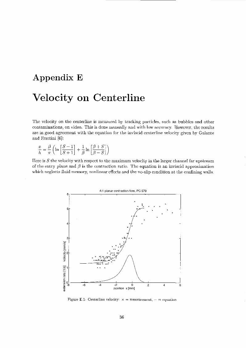
The velocity on the centerline is measured by tracking particles, such as bubbles and other contaminations, on video. This is done manually and with low accuracy. However, the results are in good agreement with the equation for the inviscid centerline velocity given by Galante and Frattini [6]:

5 = (in [-I s-1 + -ln 1 [-I) p+s h r S+l p p -s

Here is S the velocity with respect to the maximum velocity in the larger channel far upstream of the entry plane and p is the contraction ratio. The equation is an inviscid approximation which neglects fluid memory, nonlinear effects and the no-slip condition at the confining walls.

4:1 planar contraction flow, PC 570

"I 5 -

4 -

3 -

Figure E.l: Centerline velocity: x = measurement, - = equation

36

Annendix --rr -------

Comparison with 2D and 3D Newtonian Flow

In order to investigate the influence of the three dimensional character of the flow on the velocity and stress profile, a comparison is made to Newtonian flow predictions. Hereby, both two-dimensional as three-dimensional Newtonian flow is regarded. The comparisons made concern the fully developed flows at lines 1 and 2 (see figure 5.1 where also the coordinates are defined) and the pressure drop between two points even further from the contraction.

F. l 3D Velocity Field in a Fully Developed Flow

The three-dimensional velocity field in a fully developed Newtonian flow can be described by the equation [13]:

1 48(-1)P cosh(J(2p + 1 ) ~ ) cosh(S(2p + 1 ) ~ )

3- cos(v(2p + l )T) [ l - - vx - p=o ((2p + q 4 3

with v = y/h, = z / h and A = d / h . Comparing the two-dimensional and three-dimensional cross-sections of the velocity field at y=O (figure F.1) and z=O (figiire F.2), it can be see= that the difference is negligible for most of the small channel, but not for the big channel.

cross-seclion y=O: Newtonian veiociiy profile, 9 cdmin. large channel

............................

E ' $ 0 5

-10 -8 -6 -4 -2 O 2 4 6 8 10 z position [mm]

cross-section y=& Newtonian velocity profile, 9 cclmin. small channel

, i , , , , , , , , , I -10 -8 -6 -4 -2 O 2 4 6 8 10

z position [mm]

Figure F.l : cross-section at y=O - = two-dimensional, x = three-dimensional

crossbedion z=O; Newtonian veiociiy profile, 9 cdmin. large channel 1 5 ,

-4 -3 -2 -1 o 1 2 3 4 y position [mm]

cross-section z=O; Newtonian velocny profile. 9 cclrnin, small channel

-1 -0.8 -0.6 -0.4 4.2 O 0.2 0.4 0.6 0.8 1 y position [mm]

Figure F.2: cross-section at z=O - = two-dimensional, x = three-dimensional

6

5-

I 'i +++ ++

++++++ ...................................

+++++ + + + + + + +

++ ++++ +++ +++++ ++i

xxxxxxxxxxxxxxxxxxxxxxxxxxxxxxxxxxxxxxxxxxxx~xxx~x~xx~x~xxx~~xxx X xxxx

x

1 -10 -8 -6 -4 -2 O 2 4 6 8 10

z position on centerline [mm]

Figure F.3: velocity difference at the centerline y=O x = three-dimensional velocities o = three-dimensional velocity difference - = two - dimensional velocity difference

Because of the three-dimensional nature of the flow, the velocity difference experienced by the fluid at the contraction is not constant over the depth of the channel. At the centerline the velocity difference is for part of the fluid less then the 4.2 mm/s which it should be in a two-dimensional flow and for part of the fluid the difference is larger, see figure F.3.

F.2 Shear Stress in Fully Developed Regions

By calculating [V,+A,~ - V,]/Ay for all the different z-positions and calculating the mean for every y-position, the mean shear rate for both channels is known. By multiplying the shear rate with the viscosity 7 , the shear stress is known for a three-dimensional Newtonian uow. or a two-dimensional Newtonian flow the shear stress is given by -2 . Vmax . y/h2 with V,,, is 5.55 mm/s for the small channel and 1.39 mm/s for the large channel. Comparison of these shear stresses with the experimental data leads to figure F.4 and F.5. I t is remarkable that the measured data has more resemblance to the two-dimensional case than to the three- dimensional case, but the difference is in the same order of magnitude as the difference between the two- and the three-dimensional case.

n

F.3 Pressure Drop over Contraction

The pressure transducers are placed 70.5 mm upstream and 82 mm downstream of the con- traction. When considering fully developed Newtonian flow, the lower limit of the pressure drop can be calculated from:

38

. . . . small channel: 2D (dotted). 3D (line) and measured (star) pc 155

2500 I

-1 -0.8 -0 6 -0.4 -0.2 O 0.2 0.4 0.6 0.8 1 position Y/H [rnrn] C=3 5E-9, T=270 C

__.-

-1 -0.8 -0.6 -0.4 -0.2 O 0.2 0.4 0.6 0.8 1 position YIH [rnrn] CS.5E-9, TS70 C

Figure F.4: PC155: in large channel at 0.15 ml/s .. = 2D calculations, - = 3D calculations, x =measurements x = measurements

Figure F.5: PC155: riz in small channel at 0.15 ml/s .. = 2D calculations, - = 3D calculations,

Here V,,, is the maximum velocity in the small channel and h half the width of this channel. Without any flow, the pressures measured by the pressure transducers are 442 kPa upstream and 497 kPa downstream the contraction, although these pressures should be equal. This is probably caused by the way the transducers are mounted. It is assumed that this pressure difference remains constant. The measured pressure difference, corrected for this difference of 55 kPa are shown in table F.l

Table F.l: The first column is the calculated Newtonian lower limit, the second column is the measured pressure drop.

In general, the measured pressure drop is lower than the calculated pressure drop, although this calculated pressure drop is a lower limit. This could among other things be caused by:

o inaccurate pressure measurement by the pressure transducers, since these were calibrated at a different temperature. It is not known how accurate they are at 270°C.

o pressure hole effects

o inaccurate viscosity determination. There is not only an inaccuracy in the viscosity measurement, but it is also transformed to a higher temperature.

o non-isothermal effects

The variation of the measured pressure drop in time, due to an irregular flow rate caused by the gear pump, is less then two percent.

39

- Appendix G

Results of Other Control Measurements

Aside from the velocity measurements and measurements regarding the three dimensional character of the flow, some additional measurements are made. These measurements include flow rate, laser beam diameter and window signal. The field measurements (chapter 5) can also be seen as control measurements.

G . l ' Flow Rate

The flow rate is linear dependent on the speed of the gear pump, as can be seen from this table:

gear pump 5 rpm 10 rpm 15 rpm 20 rpm 25 rpm 30 rpm 35 rpm 40 rpm

extruder 1.70 2.85 4.00 5.20 6.30 7.45 8.40 9.65

flow rate 0.15 ml/s 0.29 ml/s 0.44 ml/s 0.59 ml/s 0.72 ml/s 0.88 ml/s 1.03 ml/s 1.17 ml/s

G.2 Waist of Laser Beam

In order to measure the waist of the laser beam, a razor blade was mounted on top of the flow cell. By moving the XY-tables in 2-direction (parallel to the centerline) and measuring the intensity ( IDc) , the (normalized) function of intensity versus displacement as shown in figure G.1 was found. This function was measured at three places: In the middle of the flow cell (o) and at the front (+) and the back window (x). As can be seen from the figure, the focus point of the lens was not on the centerline but about halfway between the centerline and the front window. The nominal laser beam waist without focusing lens wo equals 0.4 mm. The waist with focusing lens can be calculated from [i]:

40

waist is 0.06 rnm at z=-1 (plus), z=O (circle) and 0.08 mm at z=l (cross)

x 0.5 .

x 2 0.4

0.3

al c - -

0.2

0.1

O -0.1 -0.08 -0.06 -0.04 -0.02 O 0.02 0.04 0.06 0.08 0.1

Figure G.l: Laser beam waist at different positions

Here u11 is the waist at position z from the lens and X is the wavelength of the used light (632.8 nm). The waist w after a lens with focal length f=90 mm is 45.32 pm. With IzI is 5 and 15 mm, the waist ui1 should be respectively 0.05 and 0.081 mm. The solid lines in figure G.l are fitted on the measurements and give a waist of respectively 0.06 and 0.08 mm. The laser waist is approximately thirteen times the translation accuracy of the XY-tables. This equals 1/25 of the small channel height. Since the intensity is averaged over the whole laser beam, data becomes inaccurate at 0.08 mm distance of the wall. Given the inherent limiting resolution of a FIB system of about 100 p m [16], the system has a high spatial resolution.

G.3 Fieldwise Measurements

The isochromatics of PC155 at a flow rate of 0.88 ml/s are shown in figure 5.5. The four fringes downstream of the contraction correspond to an equivalent stress level of approximately 24 kPa. The fringe at the centerline corresponds to the zero stress level, every other fringe corresponds to a difference in equivalent stress of 7800 Pa. In chapter 5 is shown that the flow is still in the linear region for the measured material/speed combinations. Downstream of the contraction, this gives an equivalent stress level of 4 kPa at a flow rates of 0.15 ml/s. Since the first normal stress difference is negligible, the equivalent stress is about two times the shear stress (numerical value: 2.1 kPa).

41

G.4 Window signal

Since the stress optical coefficient of the window glass used is very low, the parasitic signal of the windows is very small (figure G.2.a - G.2.c). This signal is therefore negligible, unless the signal caused by the stress induced birefringence of the polymer melt is very small. This is the case at line 1, as shown in figure G.2.d: - = numerical data, + = experimental data and o=backgrounci signal windows.

I I 0 4 - 2 o 2 4

Y/h

I I - 4 - 2 o 2 4

Ylh

I I 5 - 2 0 2 4

-0.031 I O, I

J -0.021 I -1 -0.5 O 0.5 i

-0.07' -1 -0.5 O 0.5 1

O, Y(h Y!h .

a: y=-lOh b: y=O

40- -1 -0.5 O 0.5 1

Y/h

01-1 Y h 7200

0

-4 -2 o 2 4

-4 -2 o 2 4 -4 -2 o 2 4

c: y=lOh d: y=-lOh

Figure G.2: Background signd of the SF-57 windows

42

- Apnendix r --- ----- I3

Material M w Mn. PC145 14.5.103 g/mol 5.7.103 g/mol PC155 15.5.103 g/mol 6.0.103 g/mol PC158 15.8.103 g/mol 5.3.103 g/mol PC274 - 27.4.103 g/mol 11.4.103 g/mol

Materials and Equipment Used

Mz T' ~

22.1.103 g/mol 137OC 23.6.103 g/mol 135°C 23.5.103 g/mol 140°C

- 147OC

H.1 Materials Used

Table H.l: Molecular Weight Analysis and Tg

1 o'

0.1 0.1 1 o' 1 o' 0.01 1 1 OL

w ['/SI w [1/s1

1 o4

1 o3 % Y. - -0 Y B

I O 2 -

I o'

Figure H.1: Moduli and viscosity of PC155 (27OOC) Figure H.2: Moduli and viscosity of PC274 (270OC)

43

H.2 Equipment Used

e Support: Breadboard Stand: model VW-3660, Newport, 900 x 1500 cm Breadboard: XS Series, # 35, Newport, 900 x 1500 cm

I ?&iming: XY-table: compumotor 567-83-MO Parker Positioning Systems, Deadel division Compumotor 4000 Motion Controller (Parker)

e Experimental setup: Killian Extruders Inc, ser. 20236, compression ratio 3:l Zetering digital metering system: type QM, serial 6543, system 1412-15 Gear pump: Zenith, Laboratory metering unit, Model QM Flexible electric heating tape, BriskHeat, Barnstead/Thermolyne, cat. no BO0101020 3-way Valve: Butech Melt pressure transducers: Model PT467E-lM, Dynisco Temperature controller Omron E5CX Temperature controller Euroterm 91e

e Optical setup: HeNe Laser, 8 mW with Laser exciter, model 247, Spectra Physics EO-Modulator, model 370, ConOptics Arbitrary Waveform Generator: Model 395, 100 MHz synthesized, Wavetek Bias control: Conoptics, model 302 Data logger: Hydra series, 2625A, Fluke Lock-In Amplifier: Model 5302, EG&G Princeton Applied Research Oscilloscope: 9304M, 175 MHz bandwidth, 100 Msamples/s Multi meter: Model 77 series 11, Fluke NEC color CCD camera, model NX18A and lenses Navitar Sony video-cassette recorder SVO-9500 MD Sony color video printer, UP-3000, Mavigraph

44

Dataproc

% Function for calculating the retardation(De1ta) and angle(Chi), % the shear stress (Tau) and the first principal stress (Normali)

% Acquire data fiiename=input(>name file ? >,Is>); eval([>load > , filename ,>.dat>]); eval([>matrix=’, filename , ’ ; ’ I ) ; matrix=matrix(: ,i: i o ) ; corr=input(’correction factor ? ’); Ibg= .3i; % background intensity Cz3.5E-9 ; % stress-opticai coefficient d=O .O2 ; lambda=633E-9 ; % wavelength

% depth of flow channel

% Position is measured in inches. Conversion to millimeter matrix(: ,i)=matrix(: ,1)*25.4; matrix(:,2)=matrix(:,2)*25.4-1; % -i to lay zero in middle channel

% The data output of the amplifiers is 10/7.14 times too large matrix(: ,3)=matrix(: ,3)*(0.1/0.714); matrix(:,4;=matrix(:,4)*:0.:/0.7:4);

% Determine position of the measurements position=input(>variable [x/yl ? I , Is>);

if position==>x>, Y=matrix( : , i) ;

elseif position==>X>, Y=matrix(:,i); position=>x>;

else, Y=matrix(:,2); position=>y’;

end; %if

45

% Declaration of variables Icos = matrix(: ,4); Isin = matrix(: ,3); Idc = - matrix(:,5); pressure = matrix(:,7); Iout=[] ; Iin=[I : Chi=[] ; Delta=[] ; Tau=[] ; Normali=Cl;

% Calculation of Iin and Iout Iin=( Isin. / (Idc-Ibg) /torr> ; Iout=(Icos. /(Idc-Ibg)/corr) ;

% Determination of correction factors for the input % Correct for wrongly aligned optics

if position==’y’,

else,

end; %if while cor==’y’

cor=’y’ ; f=O;

cor=’n’; f=O; figure(1); clg; plot(Y, Iin, ’x’, Y, Iout, ’O’); grid;

figure(1); cïg; subplot (i, 2, i) ; plot (Y, Iin+Iout*f , ’x’ ,Y, Iout , ’O’) ; grid; subplot(l,2,2); plot(Y,Iin+Iout*f,’o’); grid; cor=input(’correction Iin with Iout [y/nl ? ’ , ’ s ’ ) ; if cor== ’ y ’

elseif cor==’Y’

end; %if end; %while

f=input(’correction factor ? ’);

f=input(’correction factor ? ’); cor=’y’;

% correct for noise signal on Iin and Iout j=min(Iin) ; k=max(Iin) ; [j ,kl bgcorl=input(’background correction Iin ? ’); Iin=Iin+ïout*f+bgcorl; j=min(Iout); k=max(Iout); cj,kj bgcor2=input(’background correction Icos ? ’) ; Iout=Iout+bgcor2;

% Determination of Chi and Delta chi = -0.5*atan(Iout./ïin); Delta1 = asin( sqrt ( (Iin. -2+Iout. -2) ) ) ; Delta = sign(-Iin).*asin(sqrt((Iin.~2+Iout.~2)));

46

% Correction for the order of Delta figure(2); clg; subplot(2,iy1); plot(real(Deltai*l80/pi) , >XI); grid; subplot(2,i,2); plot(real(Delta*l80/pi), >X I ) ; grid; axis( [I max(size(De1ta)) -100 1001); cordelta=input ( >correction delta [y/nl ? > s ) ; Del t a2=D el t a ; while cordelta==]y

npoint s=input ( which points ? cord=input(Jcorrection ? I);

porm=input ( ’plus or minus delta [p/ml ? ’ , ’ s ’ ) ; for i=npoints(i):npoints(max(size(npoints)));

) ;

if porm== p )

elseif porm==JPJ

elseif porm==’mJ

elseif porm==J#J

end; %if

Delta2(i)=cord+Delta2(i);

Delta2(i)=cord+Delta2(i);

Delta2(i)=cord-Delta2(i);

Delta2(i)=cord-Delta2(i) ;

end; %for figure(2); subplot(2,1,2); plot(real(Delta2*i80/pi), ’XI); grid; cordelta=input ( change more [y/nl ? , Is ) ; if cordelta==’Y>, cordelta= >y end %if

end %while

Delta = Delta2; Tau = (Delta. *sin (2*Chi) *lambda) / (4*pi*d*C) ; Normali = (Delta.*cos(2*Chi)*lambda)/(2*pi*d*C); figure(3); plot(real(Tau), ’XI); grid;

%‘DeleteJ positions where I sin(De1ta) I > 1 [j ,k]=f ind(sqrt (Iin. -2+Iout. -2)>1) ; Delta(j )=zeros(size(k)) ; disp(Jsqrt(Iin-2+Iout-2) > i, for elements I); j

% Necessary to plot Delta and Chi in a 3D plot cosangle=cos(Chi); sinangle=sin(Chi) ;

47

% Necessary to save the information matrix=[matrix, Iout, Iin, Chi, Delta, Tau, Normall, cosangle, sinangle] ; matrix2=[matrix(: ,1:2) Tau, Normall, Chi, Delta, Iin, Iout, pressure] ; X=matrix( : ,i) ; Y=matrix(: ,2 ) ;

% Save information if requested saveyorn=input(’save file Cy/nl ? ’ , ’ s ’ ) ; if saveyorn==’Y’,

saveyorn=’y’; end; %if if saveyorn==’y’

eval([’save ’, filename ,’ X Y Idc Iout Iin Chi Delta Tau Normall

evaï( [’save ’ , f iïename , ’ .asc matrix2 -ascii’l) cosangle sinangle corr bgcorl bgcor2’1)

end; %if

48