Charles University in Prague

Faculty of Mathematics and Physics

DOCTORAL THESIS

Martin Lanzendorfer

Flows of incompressible fluids with pressure-dependent viscosity

(and their application to modelling the flow in journal bearing)

Mathematical Institute of Charles University

Supervisor of the doctoral thesis: prof. RNDr. Josef Malek, DSc.

Study programme: Physics

Specialization: Mathematical and Computer Modelling

Prague, 2011

My deepest gratitude goes to precious teachers.

I would like to express my thanks to my supervisor, Josef Malek, for all his guidance andsupport and, in particular, for the encouragement, inspiration and enthusiasm he passes onto all his students. My gratitude belongs to Jaroslav Hron, among others for the way heimplemented his software and for his constant readiness to give advice. My co-authors, JanStebel and Adrian Hirn, are greatly acknowledged.

I greatly appreciate the opportunity to be a part of two groups with many friendly peopleand the most pleasant and relaxed atmosphere, the group of Mathematical modeling in theMathematical Institute of Charles University and the Department of Computational Methodsin the Institute of Computer Science. My thanks belongs in particular to Milan Pokorny,Miroslav Rozloznık, Zdenek Strakos and Miroslav Tuma. My special thanks go to the dearladies in the Library of ICS and to Hanka Bılkova.

To those who can benefit.To my dear Ema.

I declare that I carried out this doctoral thesis independently, and only with the citedsources, literature and other professional sources.

I understand that my work relates to the rights and obligations under theAct No. 121/2000 Coll., the Copyright Act, as amended, in particular the fact that theCharles University of Prague has the right to conclude a license agreement on the use ofthis work as a school work pursuant to Section 60 paragraph 1 of the Copyright Act.

In Prague, May 2, 2011.

Nazev prace: Proudenı nestlacitelnych tekutin s viskozitou zavislou na tlaku

(a jejich aplikace pri modelovanı proudenı v lozisku)

Autor: Martin Lanzendorfer

Pracoviste: Matematicky ustav Univerzity Karlovy

Skolitel: prof. RNDr. Josef Malek, DSc.

Abstrakt: Viskozita tekutin pri hydrodynamickem mazanı zpravidla zavisı na tlakua rychlosti smyku. Prace se zabyva ustalenym izotermalnım proudenımprave takovych tekutin. Navaze na nedavne vysledky dosazene pro prıpadhomogennıch Dirichletovych okrajovych podmınek a ukaze existenci a jed-noznacnost slabeho resenı pro okrajove podmınky pouzıvane v praktickychaplikacıch. Druha cast je pak venovana numerickym simulacım. Experi-menty naznacı uspesnost pouzite metody konecnych prvku dokud konsti-tutivnı model splnuje jista omezenı. Jak omezenı potrebna v teoretickychvysledcıch, tak ta naznacovana numerickymi experimenty umoznujı pouzıvatpresne modely maziv v jistem rozsahu tlaku a rycholsti smyku. Poslednı castprace charakterizuje tento rozsah v prıpade trech typickych reprezentantumaziv.

Klıcova slova: existence a jednoznacnost slabeho resenı, metoda konecnych prvku, viskozitazavisla na tlaku a rychlosti smyku, nestlacitelne tekutiny, hydrodynamickemazanı

Title: Flows of incompressible fluids with pressure-dependent viscosity

(and their application to modelling the flow in journal bearing)

Author: Martin Lanzendorfer

Department: Mathematical Institute of Charles University

Supervisor: prof. RNDr. Josef Malek, DSc.

Abstract: The viscosity of the fluids involved in hydrodynamic lubrication typicallydepends on pressure and shear rate. The thesis is concerned with steadyisothermal flows of such fluds. Generalizing the recent results achieved inthe case of homogeneous Dirichlet boundary conditions, the existence anduniqueness of weak solutions subject to the boundary conditions employed inpractical applications will be established. The second part is concerned withnumerical simulations of the lubrication flow. The experiments indicate thatthe presented finite element method is successful as long as certain restrictionson the constitutive model are met. Both the restrictions involved in thetheoretical results and those indicated by the numerical experiments allowto accurately model real-world lubricants in certain ranges of pressures andshear rates. The last part quantifies those ranges for three representativelubricants.

Keywords: existence and uniqueness of weak solutions, finite element method, pressure-thickening, shear-thinning, incompressible fluids, hydrodynamic lubrication

Contents

1 Introduction 1

1.1 Some open problems in hydrodynamic lubrication . . . . . . . . . . . . . . . . . 21.2 Governing equations . . . . . . . . . . . . . . . . . . . . . . . . . . . . . . . . . 81.3 Constitutive equations . . . . . . . . . . . . . . . . . . . . . . . . . . . . . . . . 91.4 Boundary conditions . . . . . . . . . . . . . . . . . . . . . . . . . . . . . . . . . 15

2 Well-posedness of the mathematical problem 19

2.1 Definition of the problem . . . . . . . . . . . . . . . . . . . . . . . . . . . . . . 202.2 Central features and discrete approximation . . . . . . . . . . . . . . . . . . . . 252.3 Well-posedness results . . . . . . . . . . . . . . . . . . . . . . . . . . . . . . . . 312.4 Auxiliary tools . . . . . . . . . . . . . . . . . . . . . . . . . . . . . . . . . . . . 38

3 Numerical method 40

3.1 Description of the numerical method . . . . . . . . . . . . . . . . . . . . . . . . 413.2 Observed behavior of the numerical method . . . . . . . . . . . . . . . . . . . . 423.3 Condition (A4) seems to determine the numerical stability . . . . . . . . . . . 43

4 Numerical simulations 47

4.1 Planar Poiseuille flow . . . . . . . . . . . . . . . . . . . . . . . . . . . . . . . . 484.2 Sliding converging surfaces . . . . . . . . . . . . . . . . . . . . . . . . . . . . . . 494.3 Planar steady flow in journal bearing . . . . . . . . . . . . . . . . . . . . . . . . 56

5 Relation between the assumed and real-world rheologies 72

5.1 Relevance of conditions (A1)–(A3) for the reference lubricants . . . . . . . . . 745.2 “Well-posed” constitutive model approximation . . . . . . . . . . . . . . . . . . 755.3 Relevance of condition (A4) for the reference lubricants . . . . . . . . . . . . . 80

6 Conclusion 87

Bibliography 89

i

Notation

N, R set of all positive integers, all real numbers

Rd Euclidean space of dimension d

Rd×dsym space of real (symmetric) square matrices

yyy ·zzz the scalar-product of vectors yyy,zzz ∈ Rd

P : Q =∑di,j=1 PijQij , the scalar-product of tensors, P,Q ∈ Rd×d

|Q| =√

Q : Q

Ω ⊂ Rd bounded domain in Rd

∂Ω ∈ C0,1 its boundary, which is Lipschitz continuous

nnn a unit outward normal vector to ∂Ω

yyyτττ =yyy − (yyy ·nnn)nnn, the tangential part of vector yyy on ∂Ω

|Ω| d-dimensional Lebesgue measure of Ω ⊂ Rd

|Γ| (d− 1)-dimensional measure of Γ ⊂ ∂Ω, Ω ⊂ Rd

Lp(Ω), ‖ · ‖p space of Lebesgue integrable functions in Ω, p ∈ 〈1,∞〉Wk,p(Ω), ‖ · ‖k,p standard Sobolev space

XXX =Xd = X × · · · ×X, for a function space X

(ξ, q)Ω =´Ωqpdxxx

(S,D)Ω =´ΩS : D dxxx

〈bbb,www〉Γ =´

Γbbb ·www dxxx

〈fff,www〉 = 〈fff,www〉W1,r(Ω)∗,W1,r(Ω)

XXX r,γ , Qr are defined on page 23

XXX r,γ, Q r

Ω∗ defined on page 26

XXX r,γh , Qrh defined on page 29

‖ · ‖(r,γ) = max‖ · ‖1,r, ‖ · ‖γ;Γ, see page 23

Cdiv(s), Cdiv(s, ν), Creg(s)

defined on page 26, see also (2.13)

βΩ∗(s, ν), β(s, ν) see (2.14)–(2.17)

βΩ(s, ν), β(s, ν) see (ISs,νΩ ) and (ISs,ν) on page 30, see also (2.22)

ii

Chapter 1

Introduction

Contents

1.1 Some open problems in hydrodynamic lubrication . . . . . . . 2

1.1.1 Journal bearings . . . . . . . . . . . . . . . . . . . . . . . . . . . . 5

1.1.2 Features neglected . . . . . . . . . . . . . . . . . . . . . . . . . . . 7

1.2 Governing equations . . . . . . . . . . . . . . . . . . . . . . . . 8

1.3 Constitutive equations . . . . . . . . . . . . . . . . . . . . . . . 9

1.3.1 On the (in)compressibility . . . . . . . . . . . . . . . . . . . . . . . 10

1.3.2 On the viscosity dependence on pressure . . . . . . . . . . . . . . . 11

1.3.3 On the viscosity dependence on shear rate . . . . . . . . . . . . . . 13

1.3.4 Three reference lubricants characterization . . . . . . . . . . . . . 14

1.4 Boundary conditions . . . . . . . . . . . . . . . . . . . . . . . . 15

1.4.1 The fluid–solid interface . . . . . . . . . . . . . . . . . . . . . . . . 15

1.4.2 The requirement to determine the level of pressure . . . . . . . . . 16

1.4.3 Permeable interfaces, artificial boundaries . . . . . . . . . . . . . . 17

1

1.1 Some open problems in hydrodynamic lubrication

The age of all kinds of powered machinery started with the Industrial Revolution about twocenturies ago, and it is not yet to pass away. By every movement in any machine a partof the consumed energy is wasted due to the relative motion of its solid components, beingdissipated partly to the generated heat and vibrations and partly to the degradation of thesolid surfaces. The very purpose of lubrication is to reduce the friction and wear by introducinga fluid medium in between the solid surfaces. The most desirable kind of lubrication is thick-film lubrication, where the surfaces are completely separated by the fluid film, the friction isminimal and there is no wear. In hydrodynamic lubrication the fluid film is generated andmaintained by the relative motion of the surfaces and due to viscous drag.

To understand the basic operation, consider an incompressible fluid introduced in between(infinite) parallel rigid plates. The distance between the plates is h and one of them is slidingrelative to the other with the velocity V . The fluid adheres to the solid surfaces and noexternal pressure gradient is imposed. Thus, a simple shear flow is generated, with the flowrate Q = V h/2 and no pressure gradient. Once the surfaces are not parallel but slightlyinclined towards one another, so that h is decreasing in the direction of the sliding, such simpleshear flow is not possible, because Q is constant due to the principle of mass conservation,while h varies. The incompressibility constraint then induces a pressure flow adding to theshear flow where h is small and lessening it where h is large. Thus, a positive (in case ofconverging surfaces) pressure peak is generated, which allows the fluid film separating thesurfaces to bear a considerable load.

In contrast to the simple shear flow, the flow involved in hydrodynamic lubrication is morecomplex. The resulting flow rate and the pressure and velocity profiles depend on variousadditional parameters, in particular on material properties of the fluid. The generated flowis essential for the operational properties of the hydrodynamical bearings. The ability ofthe mathematical models and numerical results to provide reliable predictions is of greatimportance to engineering decisions. Despite the tremendous progress during the past decades,this ability and understanding is not completea.

The processes involved in lubrication have been studied for centuries, and the lubricants, thesurfaces, the geometries and the mechanics involved have been developed and optimized. Thisthesis will not attempt to give a complete survey of what has been achieved in the field. Thereader can find the essentials and further references in many up-to-date books; to select one werefer to Szeri (1998). Instead, we will concentrate on some of the questions left open. Recentachievements in the mathematical theory allow us to revisit some fundamental issues whilethe growing availability of computer power draws our attention to new questions.

The foundations of the theoretical treatment of lubrication have been laid already by Rayleighand Stokes, and in particular by the excellent work by Reynolds (1886). Let us briefly sur-vey the basic chain of assumptions involved in deriving the standard Reynolds equation (seeRajagopal and Szeri, 2003; Szeri, 1998, for more details). Starting from the principles of con-tinuum mechanics, the conservation of mass and balances of linear and angular momenta, oneassumes that the Cauchy stress tensor of a compressible homogeneous fluid depends only on

a “. . . there has been relatively little progress since the classic Newtonian film thickness solutions towardrelating film thickness and traction to the properties of individual liquid lubricants and it is not clear atthis time that full numerical solutions can even be obtained for heavily loaded contacts using accuratemodels.” (Bair and Gordon, 2006)

2

the density and the velocity gradient. The requirement of frame indifference then implies thatthe dependence on the velocity gradient can be only through its symmetric part, while theisotropy and the assumption that the stress be linear in the velocity gradient leads to the com-pressible Navier–Stokes model. Assuming that the fluid is incompressible (and consequentlythe unspecified spherical stress enters the framework) and that the viscosity is constant, oneobtains the incompressible Navier–Stokes equations. Assuming that the body forces and theinertial forces are negligible, and comprising further that the lubrication flow takes place ina thin film between almost parallel surfaces, one concludes that the pressures can be treatedas being constant across the film, and the velocities as being parallel to the surfaces. Byintegrating the equations across the film one arrives to a single equation for the pressure: theReynolds equation.

While the above assumptions are reasonable for a large class of applications, outside this classthey could lead to serious discrepancy. In particular, this thesis will be concerned with theinstance where the pressures generated in the lubrication flow exceed the range where theviscosity can be considered independent of the pressure. This case is essential for—but notrestricted to—elastohydrodynamic lubrication, where the pressures are extremely high and theviscosity can increase by several orders of magnitude. (For simplicity, though, we will addressrather the rigid–piezoviscous regime (see Szeri, 1998), occurring in applications that exhibitpressures high enough to effectively change the lubricant’s viscosity from its inlet value, yetnot so high as to initiate significant elastic deformation in the bearing material.) Similarly, theviscosity can decrease once the shear rate is large enough, whereas the limit where the shear-thinning appears can be rather small for some technologically important fluids, or rather highfor other lubricants. The fluid properties under consideration will be specified in Section 1.3in more detail.

Once the dependence of the viscosity on the pressure is taken into account, several otherattributes of the above procedure have to be reconsidered as well. We will stick to the as-sumption that the fluid is incompressible, which can be justified even under extreme pressures,since the density of the liquids under consideration varies only slightly. However, an inter-esting question concerning the derivation of the governing equations from the principles ofcontinuum mechanics appears: whether the viscosity of an incompressible fluid can depend onthe pressure; in Section 1.2, we merely refer to a recent discussion by Malek and Rajagopalon this topic.

Having formulated a consistent constitutive relation, the subsequent important question isconcerned with the mathematical self-consistency of the resulting system of equations andwith suitable choices of boundary conditions. The existence of weak solutions for certainsubclass of the considered fluids has been established only recently. For steady flows, whichwe will be concerned with, the first existence result has been formulated by Franta et al. (2005)for the case of homogeneous Dirichlet boundary conditions. The main results of our study,presented in Chapter 2, incorporate the boundary conditions applicable to lubrication flowproblems (see Section 1.4). In this text we neglect the inertia of the fluid, such that we canfocus more on the issues related to the constitutive relation; however, the results presentedhas been achieved with the convective term included, see Lanzendorfer (2009); Lanzendorferand Stebel (2011a,b).

There is one particular distinction of piezoviscous models that is related to the level of pressurein the flow. In the case that the Dirichlet boundary conditions are prescribed on the entireboundary, the solution of the system is not determined unless an additional condition on the

3

pressure is given. As long as the viscosity is independent of the pressure, only the gradientof pressure is present in the governing equations and the pressure field is determined up toa constant: one can shift the pressure solution arbitrarily without otherwise affecting thesolution. However, once the viscosity depends on the pressure, the pressure level affects thewhole solution and has to be determined by an additional constraint (see Section 1.4 andChapter 2). We will showb that the boundary conditions allowing for free inflow and outflowwhile prescribing the traction determine the pressure level.

While in the case of a Newtonian fluid the assumption of the flow being in a thin film betweenalmost parallel surfaces (together with neglecting the body and inertial forces) has led to theconclusion that the pressure can be treated as being constant across the film and allowed toderive the Reynolds equation, one has to be careful once the viscosity depends on the pressure.Rajagopal and Szeri (2003) have pointed out that the pressure dependence of viscosity in thederivation of the governing equations for EHL cannot be only recognized a posteriori, i.e.,after the Reynolds equation has been stated under the assumption of constant viscosity. If,instead, the equation is derived consistently by taking into account the pressure dependence ofthe viscosity from the outset, then one has to involve additional simplifying assumptions andderives a modified Reynolds equation with an additional term present. In particular, once theviscosity varies rapidly with the pressure, it is no more obvious during the process whether theassumption of the pressure being constant across the field remains valid. Presumably, the fullnumerical simulation of such flows could shed some light upon this uncertainty. In general, fullnumerical simulations of lubrication flow, using accurate constitutive relations, may be of greataid to the validation of the (modified) Reynolds equations when non-Newtonian lubricants areinvolved.

In Chapters 3 and 4, we will employ a numerical approach based on the finite element dis-cretization (in two space dimensions) successfully used for flow problems with different kindsof generalized Navier–Stokes models (and for other problems). It will allow us to illustratethe basic features of some steady flows, including the flow between converging surfaces or inthe journal bearing. In particular, the possible sensitivity of the major characteristics on thepressure level (and on the related boundary conditions) will be demonstrated. The significantdepartures of the flow features when compared to the Newtonian fluid will be apparent.

We emphasize that the currently available theoretical framework allows to establish the math-ematical well-posedness only for certain subclass of fluids under consideration. Strictly speak-ing, the current theory does not cover the constitutive relations of pressure-thickening fluidswithin the entire range of pressures where the experimental data from physical measurementsare available. Once the derivative of the viscous stress tensor with respect to the pressureexceeds a certain bound, the governing equations loose their elliptic structure and there havebeen no theoretical results beyond that limit so far. One of the aims of the thesis is to examinethe behavior of the numerical simulations in this respect. The observations are summarized inChapter 3. No change in the behavior of the numerical solutions or of the numerical methodhas been found, which could be related directly to the theoretical assumptions of Chapter 2.However, (as expected) once the variations of the viscosity with pressure are large enough,the numerical method fails. A reasonably tight relation of the failure to a condition on thederivative of the viscous stress with respect to pressure has been identified. The conditionfound by numerical experiments seems identical to the assumption required for the pressurefield to be uniquely determined by the velocity field.

b The result concerning the existence and uniqueness of a weak solution subject to such boundary conditionshas been a joint work with J. Stebel.

4

Qualitatively, the limitations of the mathematical theory with respect to the real-world rela-tions between the viscosity and the pressure have been obvious by the very establishment ofthe first results. Examples of the viscosity formulae fulfilling the theoretical assumptions havebeen provided, showing that the realistic lubricants can be approximated in some range ofpressures and shear rates. It has not been clear quantitatively, however, how large the rangesof parameters in question can be. We do not provide a systematic study on this matter; inChapter 5 we examine only the three reference lubricants presented by Bair (2006) and wespecify the ranges of pressures and shear rates where the well-posedness has been proved, andthe ranges (somewhat larger), where successfull numerical solution might be expected (basedon our experience).

Note that the results presented in the thesis concern the flow of an incompressible homogeneouspressure-thickening and shear-thinning fluid in general, and they are not restricted to thelubrication problems only. Such fluid models may be applied also in other scientific areas, forexample in the modeling of the Earth’s mantle, glaciers or avalanches.

1.1.1 Journal bearings

Among the many mechanisms based on hydrodynamic lubrication, we will illustrate the pre-sented ideas on a simple model of the flow in a journal bearing. We will not discuss any detailsor particular engineering aspects, our goal is merely to motivate the more general issues bya practical example. Note that we will stay far from the full complexity of the journal bearinglubrication problem; see the next subsection for a list of the most important features excludedfrom our consideration.

The journal bearing, in the simple form we are going to look at, consists of two cylinders ofparallel eccentric axes, the outer cylinder (the bearing) being held steady while the inner (thejournal) rotates about its own axis. The lubricant is introduced into the gap between thesurfaces and is driven by the journal rotation and the viscous drag to a shearing flow. Sincethe distance between the surfaces is (due to the eccentricity) not uniform, a pressure profileis induced and a reaction force is generated, allowing the rotating journal to sustain certainload while the solid surfaces are separated by the fluid film.

A three-dimensional setting is illustrated in Figure 1.1a. The bearing can be immersed ina lubricant pool or exposed to open air, for example. One usually assumes that the lubricantis subject to an ambient pressure at the bearing ends; note in particular that some inflow andoutflow of the lubricant may occur. Various techniques are used to supply the lubricant inbetween the surfaces and avoid draining of the bearing, supply channels in the bearing bodybeing one example, as indicated in Figure 1.1b. The body of the bearing and/or the journalcan also be made of a porous material (see Figure 1.1c), which leads to a complex flow probleminvolving the lubrication flow, the flow in the porous media and at their interface. Note that inall the above mentioned settings, the inflow/outflow through (a part of) the domain boundaryis naturally present in the problem, see Subsection 1.4.3 for further discussion of the boundaryconditions.

Steady flow. In this thesis, we confine ourselves to studying steady flows in a fixed geometry;which in this context means within the geometry with a prescribed position of the journal axis.In real world, the rotating journal (when working in the hydrodynamic regime) ”floats” in the

5

nnn vvvD

nnn

ΓJ

ΓB

nnn ΓP

(a) Finite bearing.

nnn

ΓJvvvD

nnnΓB

Ω

ΓP

(b) Planar model.

ΓJ

vvvD

ΓBΩ

(c) Porous bearing.

Figure 1.1: Three examples of the journal bearing problem setting.

lubricant, being actuated by the resultant of applied load and of the forces due to the lubricantflow. Assuming that the motion of the journal axis is slow compared to the rotation speed, onecan interpret the steady flow problem as a quasi-steady approximation to the unsteady flow atcertain time and position of the journal axis. In particular, if the applied load is constant intime, the journal axis can eventually reach a steady state, where the applied load is in balancewith the force exerted by the fluid. Note that such a stable equilibrium may or may not bereached; for example, it is well-documented in the literature (e.g., see Brindley et al., 1983;Li et al., 2000b) that under the assumptions of full-film and constant viscosity lubricant, thejournal exhibits a half-speed whirl: the trajectory of the journal spirals towards the bearingwhile the angular velocity of its path approaches ω/2, where ω denotes the angular velocity ofthe journal rotation. On the other hand, steady equilibria can be reached if cavitation and/orpressure-dependent viscosity is present in the model (see Gwynllyw et al., 1996b). We willnot address questions of the dynamical behavior of the journal bearing system in this thesis.

Planar flow. If the bearing is “infinitely” long, there is no pressure relief in the axial direction.Axial flow is therefore absent and changes in shear flow must be balanced by changes incircumferential pressure flow alone. The same conditions apply in first approximation tofinite bearings of sufficient length, leading to the long-bearing approximation (see Szeri, 1998),usually applied if the length/diameter ratio L/D > 2. We remark that the aspect ratio ofindustrial bearings is customarily in the range 0.25 < L/D < 1.5, neither the short-bearing (seeibidem) nor the long-bearing approximation being applicable to such bearings. The numericalexamples in Chapter 4 will follow the long-bearing assumption and we will be concerned withthe planar flow in an eccentric annulus, see Figure 1.1b. Note that the full three-dimensionalsetting would substantially increase the CPU and memory demands, or in other words, itwould decrease the accuracy (in the sense of the size of mesh elements) accessible in ournumerical experiments.

By taking the long-bearing approximation, one immediately loses the information about thelevel of pressure (unless there is a supply channel modelled in the bearing body or the solidwalls are modelled as being porous, etc.) hitherto present in the finite-length bearing due tothe open ends. Indeed, if the flow between infinite cylinders is considered then the level ofpressure can be arbitrary. As mentioned already, this does not deserve any special treatmentas long as the viscosity does not depend on the pressure (or, similarly, as long as cavitation ofthe lubricant is not considered); while in the case with a piezoviscous lubricant an additional

6

requirement on the pressure level has to be included into the model. In the literature concernedwith the numerical simulations this deficiency of the long-bearing approximation is not alwaysemphasized. Either the mean value of the pressure over the entire domain is usually prescribed(which is not justified by the application), or the ambient pressure is prescribed at the pointof the largest gap. In Subsection 4.3.4 (see the references therein), we will illustrate ona few numerical experiments that the particular appearance of this requirement can affect thesolution of the problem considerably.

1.1.2 Features neglected

Let us emphasize the most blatant simplifications (some of them having been mentionedalready) which are not justifiable, but we take them nevertheless, merely for the sake of easierexplanation. See Szeri (1998) for more details concerning each of the following points.

• Isothermal flows will be considered (at elevated temperature, possibly). In the majorityof journal bearings, in particular in the regimes where the viscosity considerably dependson pressure, this is not a valid assumption. Note that all the energy lost by viscous forcesis dissipated into heat, which implies a significant heat production within the flow. Theviscosity depends strongly on temperature. In fact, its dependence on temperature mayaffect the solution more than its dependence on pressure.

• The entire domain is considered to be filled by the lubricant (the full-film conditions) andno cavitation nor free boundary is involved; the incompressible fluid sustains arbitrarynegative pressures. This assumption is not realistic either; the real liquids can withstandsome tensile stresses, but below certain pressure either gaseous or vapor cavitation oc-curs. “Under normal operating conditions a lubricant film . . . is expected to cavitatewithin the diverging part of the clearance, where, on the assumption of a continuouslubricant film, theory predicts negative pressures. This much is clear. Still, the subjectof considerable discussion, however, are (1) the exact position of the film-cavity interfaceand (2) the boundary conditions that apply at that interface.” (Szeri, 1998, page 98).

• The inertial forces will be neglected in this text. Concerning results on the mathematicalwell-posedness see Lanzendorfer (2009); Lanzendorfer and Stebel (2011a,b), where theconvective term is included in the governing equations. Some of the numerical simu-lations presented in Section 4.3 would not differ significantly, were the inertial forcesincluded in the model. Note, however, that in some journal bearing applications theirinclusion can have substantial effect.

• No effects of surface roughness are considered; we consider the solid surfaces as beingperfectly smooth. Moreover, in Chapter 4, we will assume that the fluid adhers to theboundary, i.e., we will prescribe the Dirichlet boundary conditions. The theoreticalresults in Chapter 2 include also Navier’s slip boundary conditions.

• The solid parts are considered to be rigid (the rigid–piezoviscous regime is assumed).This may be a valid assumption if the pressures are not too large (while the elasticmoduli of the solid parts are large enough), but this condition is never verified in thethesis.

• The lubricant is pressure-thickening and shear-thinning only. In fact, one can observeother non-Newtonian phenomena apparent in the lubrication flow, such as the visco-

7

elasticity or the normal stress differences effects, to name two. These are out of thescope of the thesis, however.

• The fluid is taken as incompressible; see Subsection 1.3.1.

1.2 Governing equations

The mathematical description of the flow is based on the following considerations. Let I ⊂ Rbe a time interval and Ω ⊂ Rd be a spatial domain occupied by the fluid. The principle ofmass conservation may be expressed in the form

ddt

ˆB

ρ dxxx+ˆ∂B

ρvvv ·nnn dxxx = 0 (1.1)

for any bounded subset B of Ω with the boundary ∂B sufficiently smooth so that the outwardnormal vector nnn may be defined. Here the time t ∈ I and the spatial position xxx ∈ Ω areindependent variables, and the density ρ = ρ(t,xxx) and the velocity vvv = vvv(t,xxx) of the fluid arestate functions. The balance of linear momentum leads to

ddt

ˆB

ρvvv dxxx+ˆ∂B

(ρvvv(vvv ·nnn)−TTnnn

)dxxx =

ˆB

ρfff dxxx, (1.2)

where fff = fff(t,xxx) is the density of an external force and T = T(t,xxx) is the Cauchy stresstensor, T = TT due to the balance of angular momentum (assuming that there are no internalcouples).

If all the quantities are sufficiently smooth, one can apply Green’s theorem to (1.1)–(1.2) andobtain

∂tρ+ div(ρvvv) = 0

∂t(ρvvv) + div(ρvvv ⊗ vvv)− div T = ρfff

in I × Ω,

where (uuu⊗ uuu)ij = uiuj and (div T)i =∑dj=1 ∂xjTij .

We confine ourselves to isothermal flows only; therefore, we do not mention the balance ofenergy. In what follows, all parameters or variables are considered at a given temperature,though this is not denoted explicitly.

For incompressible fluid we require in addition that

divvvv = 0 in I × Ω. (1.3)

If the fluid is also homogeneous then the density is a positive constant ρ ≡ ρ0 > 0 and (1.3)replaces (1.1).

We shall consider only steady flows of incompressible homogeneous fluids in the thesis and,for simplicity, we will neglect the inertial forces. Therefore, we rewrite (1.2) as

−ˆ∂B

Tnnndxxx =ˆB

fff dxxx, (1.4)

8

where fff = ρ0fff . Provided that T and fff are smooth enough, we write

divvvv = 0

−div T = fff

in Ω. (1.5)

However, instead of (1.5) which involves the derivatives of T, we will later consider rather theweak solutions of the problem, that will be properly defined in Subsection 2.1.3. Note thatthe notion of a weak solution derives directly from the integral formulation (1.4), as has beenproposedc already by Oseen (1927), see also Feireisl (2004, 2007).

1.3 Constitutive equations

For the Newtonian fluids, a linear relation between the stress and the symmetric part of thevelocity gradient D = 1

2 (∇vvv +∇vvvT ) is required, which yields (note that tr D = divvvv)

T = −pI + 2µD, tr D = 0, (1.6)

in the case of homogeneous incompressible fluid, and

T = −p(ρ)I + λ(ρ)(tr D)I + 2µ(ρ)Dδ, Dδ := D− ( 13 tr D)I

in the case of homogeneous compressible fluid. Here λ and µ are the bulk and shear moduliof viscosity. The corresponding equations of motion for Newtonian fluids are referred to asthe Navier–Stokes equations. Fluids, however, display a variety of relations between thestress and the other state variables. For a brief overview of the most frequent non-Newtonianphenomena and the corresponding fluid models see, e.g., Malek and Rajagopal (2006, 2007)and the references given there.

In this thesis, we will be concerned with the generalization of (1.6), where the viscosity dependson the pressure and the shear rate, in particular with the pressure-thickening and shear-thinning fluids. Namely, we will consider a class of incompressible fluids whose Cauchy stressis given by

T = −pI + 2η(p, |D|)D, tr D = 0, (1.7)

where |Q|2 =∑di,j=1Q

2ij . To avoid confusion in what follows, we will denote the above

generalized viscosity of an incompressible fluid by η = η(p, |D|). Note that the above class offluids excludes some phenomena that may appear in applications and will not be considered,such as the normal stress differences or viscoelastic behavior.

Note that p is the mean normal stress here, p = − 13 tr T, the reaction force due to the constraint

that the fluid is incompressible. For the derivation of the above and other constitutive relationsand for the related thermodynamic considerations see Malek and Rajagopal (2006, 2007). Wemention that (1.7) may be viewed as an implicit constitutive equation,

T− 13 (tr T)I− 2η(− 1

3 tr T, |D|)D = 0,

c Oseen (1927) only treats Navier–Stokes fluids and their linearizations. Note that the notion of solution wasnot called “weak”.

9

see ibidem and Rajagopal (2006) for a detailed discussion.

The counterpart of (1.7) in the case of a compressible fluid would be

T = −p(ρ)I + λ(ρ, tr D, |Dδ|)(tr D)I + 2µ(ρ, tr D, |Dδ|)Dδ,

(see Malek and Rajagopal, 2010). In this case p 6= − 13 tr T; but p is the thermodynamical

pressure related to ρ by the equation of state. If this relation is invertible then the viscositynaturally depends on the thermodynamical pressure:

T = −p(ρ)I + λ(ρ(p), tr D, |Dδ|)(tr D)I + 2µ(ρ(p), tr D, |Dδ|)Dδ.

If one considers a simple shear flow (e.g., between infinite parallel plates), then the (compress-ible) fluid undergoes an isochoric motion, both the pressure and density are constant withinthe flow, p(ρ) = − 1

3 tr T, and one observes (cf. (1.7))

T = −pI + 2µ(ρ(p), |D|)D. (1.8)

A natural question arises, whether it is reasonable to consider the viscosity to depend on thepressure, while considering an incompressible fluid. The answer advocated in this thesis istwofold:

First, as will be documented in this section for liquids such as lubricants, when the fluid issubject to a sufficiently large range of pressures, while the density may vary by a few percent,the viscosity can vary by several orders of magnitude. Moreover, the relative density variationswith pressure decrease with the increasing pressure; on the contrary, the relative changes ofviscosity due to the pressure are larger at larger pressures. Therefore, it is well justified tosuppose the liquid to be incompressible while at the same moment to consider its viscosity tobe pressure dependent.

Second, although this thesis considers the incompressible fluids only, we remark that an inves-tigation of compressible models related to liquid lubricants is of importance as well. In orderto provide a reliable comparison of the two (compressible and incompressible) models in thecontext of the real-world applications, a natural prerequisite is to be able to provide reliablepredictions of the flow for either of them. The theoretical results for incompressible fluids(presented in Chapter 2) as well as our numerical experiments (see Chapter 3) suffer fromcertain limitations and are applicable to real-world liquids only in a limited range of pressures(this will be documented in Chapter 5). Whether these limitations are due to insufficiency ofthe current theoretical approach only, or whether they are inherent with the assumption ofincompressibility, is not clear. Note, however, as far as concerns the rigorous analysis, that sofar there has been no results for compressible liquids analogous to those presented in Chapter 2for incompressible models (e.g., see Novotny and Straskraba, 2004).

1.3.1 On the (in)compressibility

Many experimental works on the variation of the density of liquids subject to a wide range ofpressures are reported in the 1931 book by Bridgman. We mention an empirical expression

10

0 100 200 300 400 500 600 700 800 900 10001

1.02

1.04

1.06

1.08

1.1

1.12

pressure / [MPa]

dens

ity (

rela

tive

to p

=0)

Figure 1.2: The relative density ρ(p)/ρ(0) for SQL at θ = 40 C.

(see Dowson and Higginson, 1966)

ρ(p)ρ(0)

= 1 +c1 p

1 + c2 p, c1, c2 > 0,

where ρ(0) is the density in the liquid at ambient pressure. Throughout the text, ambient pres-sure will be taken as zero; note that the atmospheric pressure is 0.1 MPa while the pressuresinvolved will be of the order of 100 MPa. Three reference liquids are accurately characterizedin (Bair, 2006), using the following two popular equations of state. The Tait equation (see thereferences in Dymond and Malhotra, 1988) writes

ρθ(0)ρθ(p)

= 1− 11 +K ′0

ln(

1 +1 +K ′0

K00 exp(−βKθ)p

)=: ωθ(p), (1.9)

where θ denotes the temperature, and where K00, K ′0, and βK are given material parameters(see Subsection 1.3.4). The Murnaghan equation (see Murnaghan, 1944) is written as

ρθ(0)ρθ(p)

=(

1 +K ′0

K00 exp(−βKθ)p

)−1/K′0

.

For illustration, we report the density (Tait equation, full line; Murnaghan equation, dotted)for squalane (SQL, see Subsection 1.3.4) in Figure 1.2. The models due to Bair (2006) areaccurate with the experimental data up to p = 400 MPa.

What we would like to point out, is that while all liquids are essentially compressible, thedensity of the liquids (such as water or common lubricants) varies slightly, say up to around10 per cent, even when subject to very high pressures, say up to 3 GPa. Since we will reportthat the viscosity can change at the same conditions by several orders of magnitude, it seemsreasonable to model such fluids as incompressible fluids with the pressure dependent viscosity.

1.3.2 On the viscosity dependence on pressure

There has been an amount of experimental work concerning the viscosity at high pressures,and we are not going to review the particular observations and models. The vast majority ofengineering literature in elastohydrodynamic lubrication, see e.g. (Szeri, 1998), relies on theexponential pressure–viscosity relation by Barus (1893)

µ = µ0 exp(αp), µ0, α > 0.

11

0 20 40 60 80 10010

−2

10−1

pressure / [MPa]

visc

osity

/ [P

a.s]

0 500 1000 150010

−2

100

102

104

106

pressure / [MPa]

Figure 1.3: The low shear viscosity µ(p) for SQL at θ = 40 C.

Other formulae can be found in the literature, which better fit experimental results; they“invariably involve an exponential relationship of sorts” (see Malek and Rajagopal, 2007,for the references). Let us remark that at the pressures involved in elastohydrodynamiclubrication, say up to 3 GPa, the viscosity may be up to 108 of its value at ambient pressure;the fluid gets close to undergoing glass transition, and the viscosity increases more rapidlythan exponentially (see Bair and Kottke, 2003).

In a recent paper by Bair (2006), three reference materials are accurately characterized for thepurposes of quantitative elastohydrodynamic lubrication considerations. In Subsection 1.3.4we will present these liquids, and we will use them as reference examples through the thesis(in particular, see Chapter 5). According to Bair, “the free volume viscosity model has beenused almost exclusively” for the accurate description of pressure dependence at high pressures;the viscosity at small shear rates

µ = µ0aθ(p)

is described by the Doolittle equation (see Doolittle, 1951) which we write including the linearcorrections due to temperature as follows:

aθ(p) = exp

BR0

1

ωθ(p)1+aV (θ−θR)1+εV (θ−θR) −R0

− 11−R0

, (1.10)

where θR = 40 C is a reference temperature, B, R0, aV , and εV given parameters, and ωθ(p)is defined by (1.9). Note that ωθ(p) has the physical meaning of the relative volume change dueto the pressure, and that the above equation is in fact the density–viscosity relation for a com-pressible fluid. However, while we will assume (approximate) that the fluid is incompressibleand its density is constant, we will consider the couple (1.9), (1.10) as a pressure–viscosityrelation, cf. (1.8).

We again illustrate in Figure 1.3 the observed relation for squalane (SQL, see Subsection 1.3.4)at θ = 40 C. The two figures differ in the range of pressures, the displayed curves being thesame. The dotted lines represent for comparison the exponential (Barus) relation, fitted tothe reference model once at lower and once at higher pressures. The reference model describesmeasured viscosities up to p = 1200 MPa accurately (see Bair, 2006).

12

10−2

100

102

104

10−2

10−1

100

101

102

103

104

|D| / [s−1]

visc

osity

/ [P

a.s]

Figure 1.4: The viscosity η(|D|) for SRM 2490 at θ = 25 C.

1.3.3 On the viscosity dependence on shear rate

We do not attept to list the many empirical models for the relation between the viscosity andthe shear rate. The behavior of shear-thinning and shear-thickening liquids typically obeysthe power-law relation (for large shear rates)

∂ ln |µD|∂ ln |D| = n

where the power-law exponent n > 0 is a material parameter. Obviously, n > 1 for shear-thickening and n < 1 for shear-thinning fluids. The simple power-law model

µ = m|D|n−1, m > 0,

is frequently considered, one of its advantages being that it allowed to find analytical solutionsto a variety of flow problems. However, it should be noted (see Bird et al., 1987) that it doesnot realistically describe the viscosity of liquids at very small shear rates.

In numerical simulations it is more standard to fit the experimental shear rate–viscosity curvesto the Carreau–Yasuda model (Carreau, 1968, 1972; Yasuda, 1979)

µ = µ∞ + (µ0 − µ∞) (1 + (|D|/G)a)(n−1)/a, µ∞ ≥ 0, µ0, G, a > 0 (1.11)

or its variants. If µ∞ > 0 then it corresponds to the second Newtonian plateau, apparentwith some important liquids such as some multigrade motor oils, see e.g. Bird et al. (1987).For illustration see Figure 1.4, where we depict the Cross model (i.e., the above equationwith a = 1 − n) for the NIST non-Newtonian Standard Reference Material, SRM 2490 Theviscosity dependence on shear rate and is drawn in a logarithmic scale. For p = 0 (full line)and p = 200 MPa (dash) the model fits to experimental data for shear rates up to 105 s−1,where the second Newtonian plateau is displayed (see Bair and Gordon, 2006). The dottedcurves show the models with µ∞ = 0, for comparison.

In order to obtain the correct shear dependence of viscosity at arbitrary temperature andpressure, a shifting rule for G is taken in the equation (see the time-temperature-pressuresuperposition or the method of reduced variables, e.g. in Bair et al., 2002; Bird et al., 1987). Thepower-law exponent n is in general independent of temperature and pressure. The reference

13

models by Bair presented in what follows are described by the Carreau equation (i.e. (1.11)with a = 2), perhaps the most frequently used shear-thinning model. Since the referenceliquids do not display the second Newtonian plateau, µ∞ = 0. We denote the equation asfollows,

ηθ(p, |D(vvv)|) = µ0 aθ(p)(1 + (bθ(p)|D(vvv)|)2

) r−22 , (1.12)

where r = n+1, and aθ(p) describes the viscosity variation due to pressure (and temperature)at small shear rates, while bθ(p) represents a shifting rule for temperature and pressure. Hereµ0 = ηθR(0, 0) is the Newtonian viscosity at reference temperature. We will usually omit thesubscript θ for the viscosity, writing only η(p, |D(vvv)|).

Bair (2006) employs two formulae for the shifting rule bθ(p) in the paper, written in ournotation as

bθ(p) =µ0 aθ(p)GR

θRρθR(0)θρθ(p)

√2 =

(µ0

GR

θRθ

(1 + aV (θ − θR)))aθ(p)ωθ(p)

√2 (1.13)

bθ(p) =µ0

GRaθ(p)1−m√2, (1.14)

the former labeled as a “standard (Ferry) shifting rule” (see also Bair et al., 2002; Ferry, 1980),

1.3.4 Three reference lubricants characterization

The presented thesis is motivated by the problem of hydrodynamic lubrication. The recentwork by Bair (2006) gives accurate material characterizations and constitutive models forthree reference liquid lubricants, selected to represent the viscosity dependence on tempera-ture, pressure and shear rate that may be observed in elastohydrodynamic lubrication. Theconsidered range of parameters, chosen to be relevant for elastohydrodynamic simulations, ismore than sufficient for our purposes (note certain limitations presented in Chapter 5). Theliquids considered are

SQL, squalane; a low-molecular-weight branched alkane, 2,6,10,15,19,23-hexamethyltetracosane;selected to represent the character of a low viscosity paraffinic mineral oil or polyal-phaolefin, it “should be Newtonian throughout the EHL inlet zone. . . ”—it does notexhibit shear-thinning up to shear rate of 109 s−1 for ambient pressure; see Figure 5.5;

PGLY, a high-molecular-weight polyglycol, poly(ethylene glycol-ran-propylen glycol); chosento represent high-molecular-weight base oils such as polyglycols, viscous polyalphaolefins,perfluorinated polyalkylethers, and silicones; it manifests apparent shear-thinning; seeFigure 5.6;

SQL+PIP, a solution of 15% by weight cis-polyisoprene in squalane; selected as a represen-tative of the polymer blended multigrade gear oils and engine oils; see Figure 5.7.

All three reference models are pressure-thickening and shear-thinning and are described bythe Carreau equation (1.12), and by the Doolittle-Tait equation (1.10) and (1.9). The shear-thinning does not display a second Newtonian plateau. The shifting rule (1.13) is used forSQL, while for PGLY and SQL+PIP (1.14) is applied. The resulting models were fitted toexperimental data for |D(vvv)| up to 105 s−1 and pressures up to (at least) 300 MPa, see thedata provided in Bair (2006); Bair et al. (2002). Note that the high shear measurements were

14

provided only for θ around 20 or at most 40 C, while we will use θ = 40 and 100 C in whatfollows (because higher temperatures can occure in lubrication problems); but it appears fromboth papers that such extrapolation can be trusted.

The material parameters for the above models of SQL, PGLY and SQL+PIP provided by Bair(2006) are summarized in Table 1.1. The viscosities depending on shear rate are presentedin Figures 5.5–5.7 (a,c) by black lines: full line for p = 0, dashed line for p = 200 MPa anddotted line for p = 400 MPa.

SQL PGLY SQL+PIP

µ0 / Pa s 0.0157 16.3 0.0711K ′0 11.74 10.80 11.29K00 / GPa 8.658 19.49 8.375βK /10−3 K−1 6.332 7.64 6.765B 4.710 3.661 4.200R0 0.6568 0.6813 0.6580aV /10−3 K−1 0.836 0.775 0.752εV /10−3 K−1 -0.7871 -1.157 -0.9599GR / MPa 6.94 0.256 0.010m – 0.10 0r 1.463 1.33 1.80

Table 1.1: Material parameters for three reference liquids,(1.12)–(1.14), θR = 40 C.

We shall employ the above three accurately characterized reference liquids particularly inChapter 5, where we will discuss (and specify quantitatively) the limitations of the currenttheoretical results and of the presented numerical method. The above models will be also usedin the numerical experiments of Chapter 4.

Let us mention the series of papers by Davies, Gwynllyw, Li and Phillips (see the bibliogra-phy) concerned with numerical simulations in a realistic journal bearing, where the authorsconsistently use another set of models fitted to the experimentally measured viscosities ofselected lubricants. Namely, the shear-thinning is described by the Cross model (eq. (1.12)with a = 1 − n) with a second Newtonian plateau (µ∞ > 0), and both a(p) and b(p) areexponentials of pressure. Note, however, that these models had been fitted to measurementsin considerably smaller ranges of parameters (see Hutton et al., 1983) than the above modelsprovided by Bair; the ranges sufficient for the purposes of journal bearing lubrication flowsimulations, but unsuited for the purposes of Chapter 5.

1.4 Boundary conditions

1.4.1 The fluid–solid interface

On the interface of the viscous fluid with the impermeable solid surface one usually assumesthat the fluid adheres to the surface, i.e., the velocity of the fluid at the boundary equals to

15

that of the solid; one prescribes the Dirichlet boundary conditions,

vvv = vvvD on some Γ ⊂ ∂Ω, (1.15)

where vvvD denotes the velocity of the solid surface. In our numerical simulations we willaccept this condition, for simplicity. Since we will consider only problems in a fixed geometry,vvvD ·nnn = 0 (where nnn denotes the unit outward normal vector on ∂Ω).

Alternatively, one can allow for the fluid to slip at the solid boundary, for example by pre-scribing the following Navier’s slip boundary condition

vvv ·nnn = 0 and − (Tnnn)τττ = α (vvv − vvvD), α ≥ 0 on some Γ ⊂ ∂Ω (1.16)

where uuuτττ := uuu− (uuu ·nnn)nnn is the projection of a vector uuu to the tangent plane, and vvvD is againthe velocity of the solid surface. The parameter α characterizes the fluid–solid interface; notethat α = 0 corresponds to the so-called free slip boundary condition, while the limit α +∞formally leads (multiplying (1.16) by 1/α first) to the Dirichlet boundary condition. Variousmore sophisticated relations between the shear stress and the slip velocity

vvv ·nnn = 0 and − (Tnnn)τττ = (bbb(vvv − vvvD))τττ , on some Γ ⊂ ∂Ω, (1.17)

can be found in literature, but we will not discuss them in detail. The assumption of slipor no-slip at solid boundary is a complex issue in the modeling of viscous fluids and theprecise circumstances determining the validity of these assumptions are subject to an unceasingconcern (e.g., see Granick et al., 2003; Neto et al., 2005).

1.4.2 The requirement to determine the level of pressure

As mentioned already in Subsection 1.1, there is a particular distinction of the piezoviscousfluid models that is related to the level of the pressure in the flow. If some of the conditions(1.15)–(1.17) is prescribed on the entire boundary (namely, if the normal part of the velocity,vvv ·nnn, is prescribed on the entire boundary) then the flow of an incompressible Newtonian fluidsubject to such boundary conditions is not determined uniquely; the same apply for the non-Newtonian models of the class (1.7) considered in the thesis. As long as the viscosity does notvary with the pressure, it is well known that the ambiguity appears in the pressure field only,namely that the pressure is defined up to a constant. Indeed, since only the pressure gradientis present in the governing equations, the addition of an arbitrary constant to the pressurefield has no other effect on the solution. This kind of non-uniqueness does not deserve anyparticular attention and is usually treated formally, by restricting the functional space wherethe pressure is sought by prescribing

ˆΩ

p dxxx = 0. (1.18)

For piezoviscous fluids this non-uniqueness has no such structure, both the pressure and thevelocity fields are undetermined and the additional constraint on the pressure level becomesan important part of the model. Regrettably, the constraint (1.18) or, in general,

ˆΩ0

p dxxx = P0, Ω0 ⊂ Ω , P0 ∈ R (1.19)

16

is not always practical from the point of view of applications; the modeller often has no hinton how to choose Ω0 and P0. One example where this issue appears has been mentioned inSubsection 1.1.1: in the standard long-bearing approximation of the journal bearing lubri-cation flow the information about the level of pressure is not present in the model; see alsoSection 4.3.

The above difficulty of the pressure level being not determined seems to be a natural conse-quence of the incompressibility assumption, in conjunction with the fluid being mechanicallyisolated in a sense. A natural question arises, whether a unique solution is provided by theboundary conditions allowing for free inflow/outflow through the boundary; see the next sub-section.

1.4.3 Permeable interfaces, artificial boundaries

There are basically two circumstances where a flow through the boundary occurs. Either theboundary describes an interface of the fluid with a permeable media (porous media, permeablemembrane) or there is no physical interface involved and an artificial boundary is introducedin order to reduce the size of the considered (computational) domain. In both cases, theboundary condition allowing for inflow and outflow involves the influence of the (usuallyunknown) motion of the fluid beyond the boundary. As such, they are not concluded fromthe physical principles only, but they result from the model reduction considerations andcan represent substantial simplification. The choice of the boundary condition at artificialboundaries is not a simple question even for a Newtonian fluid, see also the discussion inHeywood et al. (1996). Quite often the intention of the modeler is merely to ensure that“nothing (disturbing) happens” at the boundary, while it is not clear how to express thisrequirement mathematically.

For the sake of completeness, note that the Dirichlet boundary condition (1.15) is frequentlyused to prescribe the inflow in simple geometries; usually based on the expectation that thepossible disturbances to the velocity field will occur only downstream, and the assumptionthat the velocity profile on the inlet is that of a simple unidirectional steady flow (e.g., theparabolic velocity profile in the Poiseuille flow of a Newtonian fluid) and is therefore explicitlyknown. However, the precise information on the velocity profile is often not at hand, the aboveassumption does not apply for outflow conditions, and in particular, such boundary conditionsdo not determine the level of pressure in the solution, as discussed in the previous subsection.

We will consider the boundary conditions that involve the traction on the boundary, namely,

−Tnnn = bbb(xxx,vvv) on some Γ ⊂ ∂Ω, (1.20)

where bbb is the prescribed traction, which may optionally depend on the velocity. The abovecondition with bbb ≡ 000 is usually referred to as the do nothing condition. It will be shown inChapter 2 that (1.20) allows for the existence of a weak solution and, importantly, it sufficesto determine the solution uniquely.

It is worth emphasizing that the explicit knowledge of the traction on the artificial boundarymay by as unavailable as the knowledge of the velocity profile (required in the case of Dirichletboundary conditions). This is well illustrated by the example of Poiseuille flow discussed inSection 4.1: considering an artificial boundary established across the channel, perpendicular to

17

the flow, then while the normal part of the traction equals the pressure, and thus it is constantalong the boundary, the tangential part of the traction is not constant and, in particular, itdepends on the velocity profile. In such situation, it is more convenient to prescribe

vvvτττ = 000

−Tnnn ·nnn = bbb(xxx,vvv) ·nnn

on Γ ⊂ ∂Ω. (1.21)

The dependence of bbb on the velocity may be important when the inertial forces are included(we will not discuss this case, see Lanzendorfer and Stebel 2011a,b) or in case of the interfacewith some permeable media. For example,

−Tnnn ·nnn = h+ c1uuu ·nnn, c1 > 0

can be found in literature as the filtration boundary condition, with the parameters h and c1

describing the ambient pressure and the resistance to the flow. Similarly, for the flow in thedirection along the interface one may consider

−(Tnnn)τττ = c2vvvτττ c2 > 0,

which corresponds to the Beavers–Joseph(–Saffman–Jones) condition for flows past porousmedia, based on experimental observations (see Beavers and Joseph, 1967; Jones, 1973; Nield,2009; Saffman, 1971).

18

Chapter 2

Well-posedness of the mathematical

problem

Contents

2.1 Definition of the problem . . . . . . . . . . . . . . . . . . . . . 20

2.1.1 Structural assumptions (A1)–(A4) . . . . . . . . . . . . . . . . . 21

2.1.2 Boundary conditions . . . . . . . . . . . . . . . . . . . . . . . . . . 22

2.1.3 Weak formulation . . . . . . . . . . . . . . . . . . . . . . . . . . . 23

2.2 Central features and discrete approximation . . . . . . . . . . . 25

2.2.1 A priori estimates . . . . . . . . . . . . . . . . . . . . . . . . . . . 25

2.2.2 Inf–sup inequality; pressure and boundary conditions . . . . . . . . 26

2.2.3 Galerkin approximation and inf–sup conditions . . . . . . . . . . . 29

2.3 Well-posedness results . . . . . . . . . . . . . . . . . . . . . . . 31

2.3.1 Existence of discrete solutions . . . . . . . . . . . . . . . . . . . . 32

2.3.2 Uniqueness . . . . . . . . . . . . . . . . . . . . . . . . . . . . . . 33

2.3.3 Convergence of discrete solutions; existence of a weak solution . . 36

2.4 Auxiliary tools . . . . . . . . . . . . . . . . . . . . . . . . . . . 38

19

2.1 Definition of the problem

We briefly recall the governing equations introduced in the previous chapter. We shall in-vestigate the steady flow of an incompressible homogeneous viscous fluid in a bounded fixeddomain Ω ⊂ Rd, d = 2 or 3, governed by the following system of PDEs:

divvvv = 0

−div T = fff

in Ω, (2.1)

where vvv, fff , T represent the velocity, the body force and the Cauchy stress tensor, respectively.We consider

T = −pI + S, where S ≡ S(p,D(vvv)) = 2η(p, |D(vvv)|)D(vvv), (2.2)

with p the pressure, η(p, |D(vvv)|) the generalized viscosity and D(vvv) = 12 (∇vvv + ∇vvvT ) the

symmetric part of the velocity gradient. Note that S = ST and that (due to divvvv = 0)tr S = 0 such that − 1

3 tr T = p. The theory we are going to expose is based on the assumptionthat η is shear-thinning, while additional dependence of the viscosity on pressure is allowedat the same time, see below. Note that in (2.1)2 the inertial forces are neglected, whichallows us to focus on the structure of T while avoiding the mathematical difficulties due tothe convective terma.

The domain boundary is fixed, it is Lipschitz and consists of three Lipschitz partsb ∂Ω =ΓD ∪ ΓN ∪ ΓP on which we prescribe

vvv = vvvD on ΓD, (2.3a)

vvv ·nnn = vvvD ·nnn−(Tnnn)τττ =(bbb(vvv − vvvD))τττ

on ΓN , (2.3b)

−Tnnn = bbb(vvv − vvvD) on ΓP , (2.3c)

where nnn is the unit outward normal vector on ∂Ω. For any vector ωωω, we denote ωωωτττ :=ωωω − (ωωω ·nnn)nnn its tangential part. Here, vvvD is the given velocity on the boundary (velocity ofthe wall; typically, vvvD ≡ 000 on ΓN ∪ ΓP ). The function bbb ≡ bbb(xxx,vvv − vvvD) prescribes the forceon the boundary. In principal, bbb need not depend on the velocity, i.e. bbb ≡ bbb(xxx) is allowedc (seealso Lemma 1). Whether to write bbb(vvv) instead of bbb(vvv− vvvD) is a matter of personal preferenceonly.

If |ΓP | = 0 such that (2.3c) does not take effect, an additional constraint has to be posed inorder to fix the level of pressure; this is achieved by setting (cf. Bulıcek and Fiserova, 2009;

a The reader is, however, encouraged to see e.g. Bulıcek and Fiserova (2009); Lanzendorfer (2009);Lanzendorfer and Stebel (2011a,b).

b The fourth combination−Tnnn ·nnn = bbb(vvv − vvvD) ·nnn

vvvτττ = (vvvD)τττ ,

)is mentioned in Subections 1.4.3 and 4.1. We shall omit this case for better readability; the mathematicalanalysis would not encounter additional difficulties, provided that the Korn inequality was ensured.

c This is in contrast to the generalized Navier–Stokes case, where a suitable form of bbb(vvv) is needed for theexistence of solution, in order to balance the kinetic energy due to the inflow, cf. Lanzendorfer and Stebel(2011a,b).

20

Bulıcek et al., 2009b; Franta et al., 2005; Lanzendorfer, 2009)

Ω0

p dxxx = P0 (2.4)

with P0 ∈ R and Ω0 being a subset of Ω (e.g., Ω0 ≡ Ω). Without loss of generality, we setP0 = 0. For technical reasons, we shall always assume |Ω0| > 0; however, the condition (2.4)is imposed if and only if |ΓP | = 0. One our aim is to show that, instead of imposing (2.4), thepressure level is fixed by the boundary condition (2.3c) as soon as |ΓP | > 0.

In the following, the structural assumptions on S(p,D(vvv)) and the assumptions on bbb( · ) andvvvD are specified and the weak formulation of the problem is defined. The basic a prioriestimates are derived in the next section, the important relation of the inf–sup inequality tothe boundary condition (2.3c) or to the constraint (2.4) is discussed and the Galerkin discreteproblem is formulated. After giving the references to the preceeding studies, the existence ofsolution to the discrete problem, its convergence to the solution of the original problem, andthe uniqueness of both are established in Section 2.3.

2.1.1 Structural assumptions (A1)–(A4)

See the basic notation on page ii. We assume that the mapping S belongs to C1(R ×Rd×dsym; Rd×dsym), is of the form (2.2), and has the following properties:

(A1) For a given r ∈ (1, 2), there are positive constants C1, C2 and ε such that for all B,D ∈ Rd×dsym and all p ∈ R:

C1(ε2 + |D|2)r−2

2 |B|2 ≤ ∂S(p,D)∂D

· (B⊗B) ≤ C2(ε2 + |D|2)r−2

2 |B|2 ,

where (B⊗B)ijkl = BijBkl.

(A2) There is γ0 ≥ 0 such that for all D ∈ Rd×dsym and for all p ∈ R:∣∣∣∣∂S(p,D)∂p

∣∣∣∣ ≤ γ0(ε2 + |D|2)r−2

4 ≤ γ0εr−2

2 .

(A3) For a given 0 < β ≤ 1 there holds

γ0εr−2

2

(1 +

C2

C1

)< β .

Note that various values of β will be specified.

We will later (in particular in Section 2.3.2 and in Chapter 5) discuss a weaker assumption

(A4) For a given 0 ≤ γ′0 < β ≤ 1 and for all D ∈ Rd×dsym and p ∈ R:∣∣∣∣∂S(p,D)∂p

∣∣∣∣ ≤ γ′0 .

21

For every p ∈ R and D ∈ Rd×dsym (see Malek et al., 1996, Lemma 1.19 of Chapter 5) there hold(due to (A1))

|S(p,D)| ≤ C2

r − 1|D|r−1 , (2.5a)

S(p,D) : D ≥ C1

2r(|D|r − εr) . (2.5b)

Next, for all Di ∈ Rd×dsym , or vvvi ∈W1,r(Ω), i = 1, 2, we define the distances

d(D1,D2)2 := |D1 −D2|2ˆ 1

0

(ε2 + |D1 + s(D2 −D1)|2

) r−22 ds ,

d(vvv1, vvv2)2 :=ˆ

Ω

d(D(vvv1),D(vvv2))2 dxxx .

One can show that the following inequalities (see e.g. (Bulıcek et al., 2007, Lemma 1.4))

C12 d(D1,D2)2 ≤

(S(p1,D1)− S(p2,D2)

): (D1 −D2) + γ2

02C1|p1 − p2|2 , (2.6a)

|S(p1,D1)− S(p2,D2)| ≤ C2d(D1,D2) + γ0|p1 − p2| , (2.6b)

‖ε+ |D(vvv1)|+ |D(vvv2)|‖r−2r ‖D(vvv1)−D(vvv2)‖2r ≤ d(vvv1, vvv2)2 (2.6c)

hold (due to (A1), (A2)) for all pi ∈ R and Di ∈ Rd×dsym, or vvvi ∈W1,r(Ω), i = 1, 2.

2.1.2 Boundary conditions

In order to simplify the notation, we define Γ := ΓN ∪ ΓP and denote

〈bbb(uuu),ϕϕϕ〉Γ :=ˆ

Γ

bbb(uuu) ·ϕϕϕdxxx,

and treat the behaviour of bbb on ΓN and ΓP in common. We assume the following propertiesof bbb( · ).

(B1) There exists a constant γ ≥ r such that the mapping bbb( · ) : Lγ(Γ)→ Lγ′(Γ) is continuous

and bounded.

(B2) With some Bl, Bc ≥ 0,

〈bbb(uuu),uuu〉Γ ≥ Bc ‖uuu‖γγ;Γ −Bl ‖uuu‖γ;Γ for all uuu ∈ Lγ(Γ), uuu ·nnn = 0 on ΓN .

If γ > r#, then we require the coercivity: Bc > 0. Here, r# = (d−1)rd−r such that

tr W1,r(Ω) → Lr#

(Γ), where tr is the trace operator.

(B3) For all ϕϕϕ, uuu, uuun∞n=1 uniformly bounded in Lγ(Γ), such that uuun → uuu a.e. on Γ,

〈bbb(uuun),ϕϕϕ〉Γ n→∞−−−−→ 〈bbb(uuu),ϕϕϕ〉Γ,lim infn→∞

〈bbb(uuun),uuun〉Γ ≥ 〈bbb(uuu),uuu〉Γ,

and, for all ψψψ, ψψψn∞n=1 uniformly bounded in Lγ+

(Γ), γ+ > γ, such that ψψψn →ψψψ a.e. on Γ,

〈bbb(uuun),ψψψn〉Γ n→∞−−−−→ 〈bbb(uuu),ψψψ〉Γ.

22

Properties (B1)–(B3) can be ensured e.g. by the following pointwise assumptions: Let

bbb( · ) ≡ bbb(xxx, · ) = bbbc(xxx, · ) + bbbl(xxx, · ),

where, with given γ ≥ r, γ > γl, for all xxx, www ∈ Rd,

|bbbc(xxx,www)| ≤ bc(xxx) + bc|www|γ−1, with bc( · ) ∈ Lγ′(Γ), bc ≥ 0,

|bbbl(xxx,www)| ≤ bl(xxx) + bl|www|γl−1, with bl( · ) ∈ Lγ′l (Γ), bl ≥ 0,

bbbc(xxx,www) ·www ≥ Bc|www|γ , with Bc ≥ 0,

bbbl(xxx,www) ·www ≥ −bl(xxx)|www|, with bl( · ) ∈ Lγ′l (Γ).

Indeed, it is easy to verify (B1) and (B2). Also, for any uuun∞n=1, uuu, ϕϕϕ uniformly boundedin Lγ(Γ) and ψψψn∞n=1, ψψψ uniformly bounded in Lγ

+(Γ), γ+ > γ, such that uuun → uuu a.e. on Γ

and ψψψn → ψψψ a.e. on Γ,

〈bbb(uuun),ϕϕϕ〉Γ n→∞−−−−→ 〈bbb(uuu),ϕϕϕ〉Γ,〈bbb(uuun),ψψψn〉Γ n→∞−−−−→ 〈bbb(uuu),ψψψ〉Γ,〈bbbl(uuun),uuun〉Γ n→∞−−−−→ 〈bbbl(uuu),uuu〉Γ,

hold due to Vitali’s lemma and due to γl < γ and γ+ > γ, while Fatou’s lemma yields

lim infn→∞

〈bbbc(uuun),uuun〉Γ ≥ 〈bbbc(uuu),uuu〉Γ.

Further, we assume that the Dirichlet boundary data can be extended on Ω as follows.

(BD) The function vvvD in (2.3) is the trace of a function vvv0 with the following properties:

vvv0 ∈W1,r(Ω) , divvvv0 = 0 a.e. in Ω, vvv0 = vvvD on ∂Ω.

2.1.3 Weak formulation

Following the boundary conditions (2.3) with the assumptions (B1)–(BD), the constraint (2.4),and (2.5), we define the natural function spaces for the weak solution:

XXX r,γ :=www ∈W1,r(Ω) ; trwww

∣∣ΓD

= 000 , trwww ·nnn∣∣ΓN

= 0 , trwww∣∣Γ∈ Lγ(Γ)

,

Qr :=q ∈ Lr

′(Ω) ; if |ΓP | = 0 then

´Ω0q dxxx = 0

.

Let us also denote‖ · ‖(r,γ) := max‖ · ‖1,r, ‖ · ‖γ;Γ.

We use the following variant of the Korn inequality (see Lanzendorfer and Stebel (2011a)).In what follows, we will assume that the inequality (2.7) holds with IK defined by

IK :=

1, if Bc > 0,

0, if Bc = 0.

23

Lemma 1 (Korn’s inequality). Let IK ∈ 0, 1 and r > 1. Let Ω, ∂Ω and ΓN , ΓD be asabove. Assume that at least one of the following conditions apply:

i) |ΓD| > 0,ii) |ΓN | > 0 and ΓN is not a part of boundary of any rotational body in Rd,

iii) |Γ| > 0 and IK = 1.Then the following inequality holds, with cK ≡ cK(Ω,ΓD,ΓN ,ΓP , r):

‖www‖1,r ≤ cK( ‖D(www)‖r + IK‖www‖r;Γ) for all www ∈ XXX r,γ . (2.7)

Proof. The case i) with ΓD = ∂Ω, namely the inequality

c(Ω, s) ‖www‖1,s ≤ ‖D(www)‖s , for any www ∈W1,s0 (Ω), s ∈ (1,+∞),

can be found e.g. in Malek et al. (1996, Theorem 1.10 on p. 196). Its proof, in fact, coverseven i) and ii) as formulated above; it is merely to notice that a vector field of the formwww = aaa+bbb×xxx contradicts ‖www‖s = 1 under either of the assumptions www = 000 on ΓD, or www ·nnn = 0on ΓN , with ΓD, ΓN as above.

The following inequality is then stated e.g. in Bulıcek et al. (2007, Lemma 1.11),

c(Ω, s) ‖www‖1,s ≤ ‖D(www)‖s + ‖www‖2,∂Ω , for any www ∈W1,s(Ω), s ∈ (1,+∞),

but its proof again coversd also (2.7), under the assumption iii).

Let us summarize the general assumptions that will be used throughout this chapter.

Assumption 2. We assume the following: Let Ω ⊂ Rd, d = 2 or 3 is a bounded domain,∂Ω = ΓD ∪ΓN ∪ΓP where ∂Ω, ΓD, ΓN , ΓP ∈ C0,1; let Ω0 ⊂ Ω, |Ω0| > 0. For given r ∈ (1, 2)and γ0 > 0, C1, C2 > 0, let (A1)–(A2) hold true, and the boundary data (bbb( · ); Bc, Bl, γ)meet (B1)–(BD). Let fff ∈ W1,r(Ω)∗ be given. Assume that the Korn inequality (2.7) isensured, with IK = 1 allowed only if Bc > 0.

Then, we consider the following weak formulation of the problem (2.1)–(2.4).

Problem (P). Find the pair (vvv, p) such that uuu := (vvv − vvv0) ∈ XXX r,γ , p ∈ Qr and

(ξ,divvvv)Ω = 0 for all ξ ∈ Qr, (2.8a)

(S(p,D(vvv)),D(ϕϕϕ))Ω − (p,divϕϕϕ)Ω = 〈fff,ϕϕϕ〉 − 〈bbb(uuu),ϕϕϕ〉Γ for all ϕϕϕ ∈ XXX r,γ . (2.8b)

Note that 〈bbb(uuu),ϕϕϕ〉Γ =´

ΓNbbb(vvv−vvvD)τττ ·ϕϕϕτττ dxxx+

´ΓPbbb(vvv−vvvD) ·ϕϕϕdxxx for all uuu,ϕϕϕ ∈ XXX r,γ , cf. (2.3).

All integrals in (2.8) are finite, due to (2.5a) and (BD), (B1).

dActually, for any |Γ| > 0, Γ ⊂ ∂Ω not lying on boundary of any rotational body, one can also see thatc(Ω,Γ, s) ‖www‖1,s ≤ ‖D(www)‖s + ‖www ·nnn‖s;Γ.

24

2.2 Central features and discrete approximation

2.2.1 A priori estimates

In order to motivate what follows, let us briefly describe the basic structure of the problem byoutlining the a priori estimates. Testing the weak formulation by solution, i.e. setting ξ := p

in (2.8a) and ϕϕϕ := uuu in (2.8b) and summing the equations, recalling that divvvv0 = 0, we obtain

(S(p,D(vvv)),D(uuu))Ω + 〈bbb(uuu),uuu〉Γ = 〈fff,uuu〉.

Applying (2.5) and the Holder and Young inequalities we observe

(S(p,D(vvv)),D(vvv)−D(vvv0))Ω ≥ C12r (‖D(vvv)‖rr − |Ω|εr)− C2

r−1‖D(vvv0)‖r‖D(vvv)‖r−1r

≥ C12r ‖D(uuu)‖rr − C(1 + ‖D(uuu)‖r−1

r ) ≥ C‖D(uuu)‖rr − C.

By C we always denote generic constants, positive and finite. Above, C depend on Ω, r, C1,C2, ε and ‖vvv0‖1,r.

Next, we apply (B2) and distinguish two cases: If Bc = 0 then we require γ ≤ r# andIK = 0 in the Korn inequality (2.7) (the cases i) and ii) in Lemma 1). Using the embeddingtr W1,r(Ω) → Lγ(Γ) and (2.7), we obtain

C ‖D(uuu)‖rr + 〈bbb(uuu),uuu〉Γ ≥ C ‖uuu‖r1,r −Bl ‖uuu‖γ;Γ ≥ C ‖uuu‖r1,r − C.

If Bc > 0 then we do not need the embedding and we also allow for IK = 1 in (2.7). Sinceγ > r, we obtain

C ‖D(uuu)‖rr + 〈bbb(uuu),uuu〉Γ ≥ C ‖D(uuu)‖rr + (Bc2 ‖uuu‖γγ;Γ + C ‖uuu‖rr;Γ − C) ≥ C ‖uuu‖r1,r + Bc

2 ‖uuu‖γγ − C.

Here, C depend also on ΓD, ΓN , ΓP , γ, and Bl, Bc.

By combining the inequalities above and using again (2.5a) to estimate ‖S(p,D(vvv))‖r′ , wearrive at the a priori estimate

‖vvv‖1,r + ‖S(p,D(vvv))‖r′ + ‖uuu‖γ;Γ ≤ Kvvv, (2.9)

with Kvvv depending on Ω, ΓD, ΓN , ΓP , r, γ, C1, C2, ε, Bc, Bl, ‖vvv0‖1,r and ‖fff‖W1,r(Ω)∗ .

Note that since the pressure p is involved in the nonlinear term S(p,D(vvv)), we need also somea priori bound of the pressure. Using the last estimate and applying (2.5a), (B1) and theHolder inequality to the equation (2.8b), we observe

(p,divϕϕϕ)Ω ≤ ‖S(p,D(vvv))‖r′‖D(ϕϕϕ)‖r + ‖fff‖W1,r(Ω)∗‖ϕϕϕ‖1,r + ‖bbb(uuu)‖γ′;Γ‖ϕϕϕ‖γ;Γ

≤ C (‖ϕϕϕ‖1,r + ‖ϕϕϕ‖γ;Γ)

for all ϕϕϕ ∈ XXX r,γ . Suppose that we can find ϕϕϕ ∈ XXX r,γ and β > 0 such that

β ‖p‖r′ (‖ϕϕϕ‖1,r + ‖ϕϕϕ‖γ;Γ) ≤ (p,div ϕϕϕ)Ω . (2.10)

25

This finally gives us the desired a priori bound

β ‖p‖r′ ≤ Kp, (2.11)

with Kp depending on Kvvv, ‖fff‖W1,r(Ω)∗ and on sup‖uuu‖γ;Γ≤Kvvv ‖bbb(uuu)‖γ′;Γ, which is bounded dueto (B1).

Note that (2.9) and (2.11) are consistent with the choice of the spaces XXX r,γ and Qr. We alsoremark that while deriving the estimates, Assumption (A2) has not been used; the viscosity–pressure dependence has been controlled by (A1).

Most importantly, mind that (2.11) relies on the inequality (2.10). It may seem that we didnot encounter the requirements concerning how the pressure level is fixed (i.e. the restrictions(2.3c) or (2.4)); this issue is also connected with the inequality (2.10).

2.2.2 Inf–sup inequality; pressure and boundary conditions

The inequality (2.10) is the result of Corollary 6 proven below, which is crucial to the analysisof (P). Note that the corollary not only allows for the a priori estimate (2.11), but it is usedseveral more times in the sequel analysis. Its proof reveals the relation between the boundaryconditions and the pressure.

First, let us define the “inner flow” spaces

XXX r,γ:= www ∈ XXX r,γ ; trwww ·nnn

∣∣Γ

= 0 ,Q r

Ω∗ := Lr′

0;Ω∗(Ω) = q ∈ Lr′(Ω) ;

´Ω∗q dxxx = 0,

where Ω∗ ⊂ Ω, |Ω∗| > 0. Note that if |ΓP | = 0 then (XXX r,γ,Q r

Ω0) = (XXX r,γ ,Qr). Note that for

any www ∈ XXX r,γthere holds

´Ω

divwww dxxx =´∂Ωwww ·nnndxxx = 0.

The basic tool related to the inequality (2.10) is the following

Lemma 3. Let Ω, ΓD, Γ be as in Assumption 2, let s ∈ (1,∞) and ν ∈ 〈1,∞〉. Then thereexists a continuous linear operator B : Ls0(Ω) → XXX s,ν

and a constant Cdiv(s, ν) (dependingalso on Ω and Γ) such that for all f ∈ Ls0(Ω):

div(Bf) = f a.e. in Ω, ‖Bf‖(s,ν) ≤ Cdiv(s, ν)‖f‖s. (2.12)

Proof. The following result is well-known: there exists a continuous linear operator B :Ls0(Ω)→W1,s

0 (Ω) such that for all f ∈ Ls0(Ω):

div(Bf) = f a.e. in Ω, ‖Bf‖1,s ≤ Cdiv(s)‖f‖s,

where Cdiv(s) depends on s and Ω. See Novotny and Straskraba (2004, Lemma 3.17) orAmrouche and Girault (1994); Bogovskii (1980). Since W1,s

0 (Ω) ⊂ XXX s,ν, this implies that

(2.12) holds, e.g., with Cdiv(s, ν) := Cdiv(s).

While the above proof is based on the properties of the divergence operator on W1,s0 (Ω), it is

worth noting that an alternative approach has been used in the case of Navier’s slip boundaryconditions, i.e., with |ΓD| = 0, using the solution to the Neumann problem with the Laplace

26

operator, cf. (1.30)–(1.33) in Bulıcek et al. (2007) or (2.24)–(2.27) in Bulıcek et al. (2009b).One can consider a linear operator N−1

Ω : Ls0(Ω) → u ∈ W2,s(Ω), ∇u ·nnn = 0 on ∂Ω anda constant Creg(s) (depending also on Ω) such that for all f ∈ Ls0(Ω),

div(∇N−1Ω (f)) = f a.e. in Ω, ‖∇N−1

Ω (f)‖1,s ≤ Creg(s)‖f‖s.

It could be interesting to specify the operator B more precisely in our setting (which combinesthe no-slip and slip boundary parts), and to estimate the optimal value of Cdiv(s, ν), but wedo not address that question here. One easily observes

Creg(s) ≤ Cdiv(s, ν) ≤ Cdiv(s), for all s ∈ (1,∞), ν ∈ 〈1,∞〉. (2.13)

We use the above lemma to show the inequality more fitting to our needs (especially to thediscrete spaces discussed later) in the following

Corollary 4. Let Ω, ΓD, Γ be as in Assumption 2 and Ω∗ ⊂ Ω, |Ω∗| > 0. For any s ∈ (1,∞)and ν ∈ 〈1,∞〉 there exists a constant βΩ∗(s, ν) (depending also on Ω, Ω∗ and Γ) such that

0 < βΩ∗(s, ν) ≤ infq∈Q sΩ∗

supwww∈XXX s,ν

(q,divwww)Ω

‖q‖s′‖www‖(s,ν). (2.14)

Proof. For any q ∈ Q s

Ω∗ , set q = q0 + (fflΩq dxxx), so that q0 ∈ Ls

′

0 (Ω). (Note that if Ω∗ = Ω thenq = q0.) Recall Lemma 3 and set www := B

(|q0|s

′−2q0−fflΩ|q0|s

′−2q0 dxxx), implying that www ∈ XXX s,ν

and (q,divwww)Ω = ‖q0‖s′

s′ . Similarly as in Bulıcek et al. (2009b) we observe by contradictionand since

fflΩ∗q dxxx = 0 and

fflΩq0 dxxx = 0 that ‖q‖s′ ∼ ‖q0‖s′ , with the constants depending

on Ω, Ω∗ and s. Hence, ‖q0‖s′

s′ ≥ C ‖q‖s′s′ and ‖|q0|s′−2q0 −

fflΩ|q0|s

′−2q0 dxxx‖s ≤ C ‖q‖s′−1s′ ,

concluding that (2.14) holds with βΩ∗(s, ν) depending on Ω, Ω∗, Γ, s and ν.

Remark 5. For s = 2, we observe that

βΩ0(2, ν) ≥ |Ω0||Ω| βΩ(2, ν) ≥ |Ω0|

|Ω|1

Cdiv(2, ν)≥ |Ω0||Ω|

1Cdiv(2)

. (2.15)

Proof. We repeat the procedure above. Same as in Bulıcek et al. (2009b), since´Ω0q dxxx = 0,

we note that

‖q0‖22 = ‖q‖22 −1|Ω|

(ˆΩ

q dxxx)2

= ‖q‖22 −1|Ω|

(ˆΩ\Ω0

q dxxx

)2

≥ |Ω0||Ω| ‖q‖

22

and that ‖q‖2 ≥ ‖q0‖2. Since www = B(q0), and due to (2.13), the assertion follows.

In the case |ΓP | = 0, i.e. if no free flow through the boundary is allowed, Corollary 4 withΩ∗ = Ω0 ensures the important inequality (2.10). We can also see why the constraint (2.4) isrequired: obviously,

infq∈Ls′ (Ω)

supwww∈XXX s,ν

(q,divwww)Ω

‖q‖s′‖www‖(s,ν)= 0.

However, if |ΓP | > 0 then the constraint (2.4) is redundante, as shows the following general-ization of Corollary 4:

e And, as follows later from Theorem 12, it is inappropriate then.

27

Corollary 6. Let Ω, ΓD, ΓN and ΓP be as in Assumption 2. For any s ∈ (1,∞) and ν ∈〈1,∞〉 there exists a constant β(s, ν) (depending also on Ω, Ω0, ΓN and ΓP ) such that

0 < β(s, ν) ≤ infq∈Qs

supwww∈XXX s,ν

(q,divwww)Ω

‖q‖s′‖www‖(s,ν). (2.16)

Proof. Since if |ΓP | = 0 then (XXX s,ν,Q s

Ω0) = (XXX s,ν ,Qs), the assertion follows from Corollary 4

by setting β(s, ν) := βΩ0(s, ν). It remains to show (2.16) for |ΓP | > 0, see e.g. Haslinger andStebel (2011); Hirn et al. (2010).

For any q ∈ Qs = Ls′(Ω), we write q = q0+(

fflΩq dxxx). Since q0 ∈ Ls

′

0 (Ω) = Q s

Ω and due to (2.14),there exists www0 ∈ XXX

s,ν, ‖www0‖(s,ν) = 1, such that βΩ(s, ν)‖q0‖s′ ≤ (q0,divwww0)Ω = (q,divwww0)Ω.

Since ΓP ∈ C0,1, |ΓP | > 0, there exists some ξξξ ∈ XXX s,ν such that´Ω

div ξξξ dxxx =´

ΓPξξξ ·nnndxxx = 1.

Taking

www := www0 + δ sign(fflΩq dxxx)ξξξ, with δ :=

βΩ(s, ν)|Ω|1/s′

1 + |Ω|1/s′‖div ξξξ‖s,

we observe www ∈ XXX s,ν , and by using ‖q‖s′ ≤ ‖q0‖s′ + |Ω|1/s′ |fflΩq dxxx| we obtain:

(q,divwww)Ω = (q,divwww0)Ω + δ sign(fflΩq dxxx) (q0,div ξξξ)Ω + δ|

fflΩq dxxx| (1,div ξξξ)Ω

≥ βΩ(s, ν)‖q0‖s′ − δ‖q0‖s′‖ div ξξξ‖s + δ|fflΩq dxxx|

≥ βΩ(s, ν)1 + |Ω|1/s′‖div ξξξ‖s

‖q‖s′ .

Finally, since ‖www‖(s,ν) ≤ 1 + δ ‖ξξξ‖(s,ν) we conclude that (2.16) hold e.g. with

β(s, ν) :=βΩ(s, ν)

1 + |Ω|1/s′‖ div ξξξ‖s + βΩ(s, ν)|Ω|1/s′‖ξξξ‖(s,ν)

. (2.17)

Remark 7. In some previous studies (see Lanzendorfer and Stebel, 2011a,b), the inf–supinequality has not been formulated, but (for |ΓP | > 0) a modified operator B is applied instead:Starting e.g. with B from Lemma 3, one considers Bf := B

(f − (

´Ωf dxxx) div ξξξ

)+ (

´Ωf dxxx)ξξξ

with the estimate ‖Bf‖1,s + ‖Bf‖ν;Γ ≤ Cdiv(s, ν) ‖f‖s (cf. Lemma 2.4 in Lanzendorfer andStebel (2011b) for the case |ΓN | = 0). We remark that this approach is equivalent: similarlyas in Remark 5, with β(s, ν) defined by (2.17) one observes

β(s, ν) =1

Cdiv(s, ν).

Indeed: Obviously, B : Qs →XXX s,ν and, for any f ∈ Qs = Ls′(Ω),

‖Bf‖(s,ν) ≤ Cdiv(s, ν)‖f − (´Ωf dxxx) div ξξξ‖s + |

´Ωf dxxx| ‖ξξξ‖(s,ν) ≤ Cdiv(s, ν)‖f‖s,

whereCdiv(s, ν) := Cdiv(s, ν)(1 + |Ω|1/s′‖ξξξ‖s) + |Ω|1/s′‖ξξξ‖(s,ν).

Setting www := B(|q|s′−2q) we easily observe

(q,divwww)Ω

‖q‖s′‖www‖(s,ν)≥ 1

Cdiv(s, ν).

28

Corollary 6 provides (2.10), implying the a priori estimates (2.9), (2.11) with β := β(r, γ) forProblem (P).

2.2.3 Galerkin approximation and inf–sup conditions

For given h > 0, let XXXh, Yh be finite-dimensional spaces and let

XXX r,γh := XXXh ∩XXX r,γ , Qrh := Yh ∩Qr.

At the moment, we do not specify the choice of XXXh, Yh and do not impose any particularmeaning on the parameter h (although the inspiration by finite elements is obvious). We onlyrequire that the families XXX r,γh h>0, Qrhh>0 are dense in XXX r,γ , Qr, respectively, i.e.

limh0

infwwwh∈XXX r,γh

‖www −wwwh‖1,r = limh0

infqh∈Qrh

‖q − qh‖r′ = 0 for all www ∈ XXX r,γ and q ∈ Qr.

(2.18)

The Galerkin approximation of (P) consists in replacing XXX r,γ , Qr by their finite dimensionalsubspaces XXX r,γh , Qrh:

Problem (Ph). Find (vvvh, ph) such that uuuh := (vvvh − vvvh,0) ∈ XXX r,γh , ph ∈ Qrh and

(ξh,divvvvh)Ω = 0 for all ξh ∈ Qrh, (2.19a)

(S(ph,D(vvvh)),D(ϕϕϕh))Ω−(ph,divϕϕϕh)Ω = 〈fff,ϕϕϕh〉−〈bbb(uuuh),ϕϕϕh〉Γ for all ϕϕϕh∈XXX r,γh . (2.19b)

Here, vvvh,0 is an approximation of the Dirichlet data which satisfies

(ξh,divvvvh,0)Ω = 0 for all ξh ∈ Qrh and limh0‖vvv0 − vvvh,0‖1,r = 0. (2.20)

For example, vvvh,0 ∈ XXXh is typical in the finite elements setting; but one can also simplyconsider vvvh,0 = vvv0.

Let us consider the a priori estimates for the discrete problem (Ph). Obviously, since we cantest the equations (2.19) by the discrete solution, we obtain exactly (2.9) also for the discretesolution. However, in order to obtain the pressure estimate we need to ensure (2.10) on thediscrete level, i.e. with ϕϕϕ ∈ XXX r,γh . In contrast to the continuous level, where (2.10) is ensuredby Corollary 6, here the inequality involves an additional constraint for the choice of discretespaces XXXh and Yh.

In the following, we require for given s ∈ (1,∞) and ν ∈ 〈1,∞〉 that the families of spacesXXX s,νh h>0, Qshh>0 satisfy the discrete inf–sup condition, cf. (2.16):

(ISs,ν) There exists a constant β(s, ν) independent of h such that

0 < β(s, ν) ≤ infq∈Qsh

supwww∈XXX s,νh

(q,divwww)Ω

‖q‖s′‖www‖(s,ν).

The value of β(s, ν) (and existence of such positive number) depends on the particular choiceof the discrete spaces XXXh, Yh. In the finite element discretization, this is an important issue.

29

For the purpose of our existence analysis, namely in the proof of Corollary 15, we utilizefavourable Galerkin spaces for which the value of the discrete β (almost) equals to β of thecontinuous level, see Lemma 9 below. Let us emphasize that the value of β represents an im-portant constraint on the model, see the assumptions of Theorems 12, 14 and of Corollary 15.In view of this, it is worth noting (from (2.17) in the case |ΓP | > 0 and from (2.15) in the case|ΓP | = 0) that β(s, ν) can possibly be much less then βΩ(s, ν) (although (2.17) and (2.15)prove only the lower bound for β(s, ν)).

Therefore, in a hope that βΩ(s, ν) ≥ β(s, ν), we formulate also the following variant of thediscrete inf–sup condition, cf. (2.14):

(ISs,νΩ ) There exists a constant βΩ(s, ν) independent of h such that

0 < βΩ(s, ν) ≤ infq∈Yh∩Q

sΩ

supwww∈XXXh∩XXX

s,ν

(q,divwww)Ω

‖q‖s′‖www‖(s,ν).

Remind that Q s

Ω = Ls0(Ω) and note that if |ΓP | = 0 and Ω0 = Ω then (ISs,νΩ ) is exactly(ISs,ν). In general, (ISs,νΩ ) need not be implied by (ISs,ν) and vice versa.

In Theorem 14 we will apply (ISs,νΩ ) by means of the following

Remark 8. Let r ∈ (1, 2), ν ∈ 〈1,∞〉 and let (IS2,νΩ ) hold. Then, for all q ∈ Qrh,

βΩ(2, ν)(‖q‖2 − |Ω|1/2|

fflΩq dxxx|

)≤ supwww∈XXXh∩XXX

2,ν

(q,divwww)Ω

‖www‖(2,ν). (2.21)

Indeed: For arbitrary q ∈ Qrh ⊂ L2(Ω), we can write q = q0 + (fflΩq dxxx), wheref q0 ∈ Yh ∩

L20(Ω) = Yh ∩ Q

2

Ω. Since ‖q‖2 ≤ ‖q0‖ + |Ω|1/2|fflΩq dxxx|, and XXX 2,ν ⊂ XXX 2,ν , we obtain (2.21)

from (IS2,νΩ ).

Lemma 9. Let Ω, ΓD, ΓN , ΓP , Ω0 and r, γ be as in Assumption 2. Then, for any δ > 0(small), there exists a family of finite-dimensional spaces XXXhnhn>0, Yhnhn>0, hn 0,satisfying (2.18) and (ISr,γ), (IS2,γ

Ω ) with

β(r, γ) ≥ β(r, γ)− δ and βΩ(2, γ) ≥ βΩ(2, γ)− δ. (2.22)

Proof. Consider arbitrary hn 0, n = 1, . . .. Since XXX 2,γ, XXX r,γ , Qr are separable Banach

spaces with the bases wwwn∞n=1, wwwn∞n=1, qn∞n=1, respectively, and since XXX 2,γ ⊂ XXX r,γ , wecan define Galerkin spaces by XXXm := spanwwwi,wwwimi=1 and Y n := spanqini=1, m,n = 1, . . .,obviously allowing for the density (2.18). In order to ensure the discrete inf–sup conditionswith (2.22), we only need to choose suitable pairs of the spaces, i.e. to any discrete pressurespace to assign a rich enough discrete velocity space. We show this only for (IS2,γ

Ω ) and(2.22)2, the inclusion of (ISr,γ) is obvious.

Due to the density and Corollary 4, for any q ∈ Q 2

Ω there exists k(q) such that

βΩ(2, γ)− δ ≤ supwww∈XXXk(q)∩XXX 2,γ

(q,divwww)Ω

‖q‖2‖www‖(2,γ)

f Here we silently assume that constants belong to Yh.

30

(we choose minimal such k(q)). For n fixed, define m(n) := supq∈Y n∩Q 2Ωk(q). It is easy to

see that Yhn := Y n and XXXhn := XXXm(n) satisfy (IS2,γΩ ) and (2.22)2. It remains to prove that

m(n) is finite, which we show by contradiction: Let m(n) be infinite, then we find a sequenceqj ∈ Y n ∩Q

2

Ω, ‖qj‖2 = 1, j = 1, . . ., such that k(qj) > j and

supwww∈XXXj∩XXX 2,γ

(qj ,divwww)Ω

‖www‖(2,γ)< βΩ(2, γ)− δ.

Since Y n is of finite dimension, we find some q ∈ Y n∩Q 2

Ω, ‖q‖2 = 1, and a subsequence ji > i

such that ‖qji − q‖2 < δ/2 for i = 1, . . .. But then,

supwww∈XXXi∩XXX 2,γ

(q,divwww)Ω

‖www‖(2,γ)< βΩ(2, γ)− δ/2

holds for any i = 1, . . ., which combined with the density and Corollary 4 gives the contradic-tion.

2.3 Well-posedness results

Despite of the wide range of important applications, the rigorous mathematical analysis ofthe incompressible fluid flow models with the viscosity depending on the pressure has notattracted much research activity until the turn of century. The earlier results (by Gazzola,1997; Gazzola and Secchi, 1998; Renardy, 1986), concerned with the viscosity depending solelyon the pressure, established the existence for a short time interval and due to small data only.For the stationary problem, Renardy (1986) notes that the equations lose the ellipticity unlessthe derivative of the viscosity with respect to pressure is bounded by reciprocal of eigenvaluesof D(vvv). For fluids whose viscosity depends solely on pressure or grows superlinearly withpressure, as far as no severe restrictions on the data size or time interval are imposed, thewell-posedness of the mathematical problem is not known.

An opening result appeared in Malek et al. (2002) and Hron et al. (2003), where the viscositiesdepending both on the pressure and shear rate—their structure given by Assumptions (A1)and (A2)—were considered, allowing for the global and large data existence results. Theseresults, established for periodic boundary conditions, were then extended to unsteady flowsin bounded domains subject to Navier’s slip boundary conditions in Bulıcek et al. (2007),see also Malek and Rajagopal (2007) for more references. The well-posedness of the steadyproblem (Problem (P) with the convective term included) was first studied by Franta et al.(2005) for the homogeneous Dirichlet boundary conditions. This result was generalized tocover the non-homogeneous Dirichlet data in Lanzendorfer (2009). The problem with theboundary condition (2.3c) allowing for free flow through the boundary present, i.e. the case|ΓP | > 0, was studied in Lanzendorfer and Stebel (2011a,b).

We merely mention that the presented theoretical framework allowed to show also the a prioriestimates of the discretization error, see Hirn et al. (2010) for more details.

In this section, we show the existence of discrete solutions to (Ph) (in Theorem 11), we discussthe conditions guaranteeing the uniqueness of solutions both to (P) and (Ph) (in Theorems 12and 13), and we finally establish the existence of a weak solution to (P) as the limit of thediscrete solutions (in Corollary 15).

31

Compared to the previous works Lanzendorfer (2009); Lanzendorfer and Stebel (2011a,b), weslightly relax the restriction on γ0 when showing the existence. In fact, we bring its range backto that allowed in Franta et al. (2005) for the case |ΓP | = 0 and Ω0 = Ω, cf. Corollary 15 and(2.15), (2.17). The same was, however, not acquired for the uniqueness result, see Theorem 12.Our procedure also allows for r ∈ (1, 2); but this is merely because the convective term is notpresent in our model.

The basic structure of the proof of existence of a weak solution to the steady problem inthe above mentioned papers followed the procedure by Franta et al. (2005): First, a quasi-compressible approximation to (P) was established (by the Galerkin method), and later itsconvergence (on the continuous level) to the “incompressible” solution to (P) was shown. Notethat here, since our concern lies with the discretization, the procedure is slightly different: theweak solution is established directly as a limit of discrete solutions and these discrete solutionsalready satisfy the incompressibility constraint.

2.3.1 Existence of discrete solutions

Remark 10. Let Assumption 2 hold. Let (XXX r,γh ,Qrh) fulfill (ISr,γ) with β(r, γ) > 0 arbitrary.Then, all (vvvh, ph) the solutions to (Ph) satisfy the a priori estimates

‖vvvh‖1,r + ‖S(ph,D(vvvh))‖r′ + ‖uuuh‖γ;Γ ≤ Kvvv and β(r, γ) ‖ph‖r′ ≤ Kp, (2.23)

with the constants Kvvv and Kp from (2.9) and (2.11).

Indeed: The estimates derives in exactly the same way as (2.9), (2.11) in Section 2.2.1.

Theorem 11 (Existence of discrete solutions). Let Assumption 2 hold, let XXX r,γh and Qrh fulfil(ISr,γ) with β(r, γ) > 0 arbitrary. Then there exists a discrete solution to (Ph).

Proof. For any δ > 0 (small), we consider the following quasi-compressible approximate prob-lem: Find (vvvδh, p

δh) such that uuuδh := (vvvδh − vvvh,0) ∈ XXX r,γh , pδh ∈ Qrh and

δ(pδh, ξh

)Ω

+(ξh,divvvvδh

)Ω

= 0 for all ξh ∈ Qrh(S(pδh,D(vvvδh)),D(ϕϕϕh)

)Ω−(pδh,divϕϕϕh

)Ω

= 〈fff,ϕϕϕh〉 − 〈bbb(uuuδh),ϕϕϕh〉Γ for all ϕϕϕh ∈ XXX r,γh .

The inserted term δ(pδh, ξh

)Ω

ensures the coercivity of the equations with respect to thepressure and allows to use the Brouwer fixed-point theorem to establish the solution to (Ph).Indeed, setting (ϕϕϕh, ξh) := (uuuδh, p

δh) and following the same steps as when deriving the a priori

estimates (2.9), we verify the assumptions of Corollary 17 and obtain the solution (vvvδh, pδh) to

the approximate problem and the a priori bound

δ‖pδh‖22 + ‖vvvδh‖r1,r + ‖S(pδh,D(vvvδh))‖r′r′ ≤ Kvvv and β(r, γ) ‖pδh‖r′ ≤ Kp,

where we have also used (ISr,γ), cf. (2.11).

32

The uniform bounds and the fact that XXX r,γh and Qrh are of finite dimension imply that thereis vvvh = vvvh,0 + uuuh, uuuh ∈ XXX r,γh and ph ∈ Qrh such that (for some sequence δn 0)

vvvδnh → vvvh strongly in W1,r(Ω),

uuuδnh → uuuh strongly in Lγ(Γ),

pδnh → ph strongly in Lr′(Ω),

S(pδnh ,D(vvvδnh ))→ S(ph,D(vvvh)) strongly in Lr′(Ω)d×d,

bbb(uuuδnh )→ bbb(uuuh) strongly in Lγ(Γ).

Consequently (vvvh, πh) is a solution to (Ph).

2.3.2 Uniqueness

In the uniqueness considerations, Problems (P) and (Ph) can be treated identically, as willbecome obvious in a moment. One might have noticed that Assumption (A2) was not utilizedto show the a priori estimates nor to prove the existence of discrete solutions in the previoussection. Its function appears right below.

First, we may ask whether the pressure is determined uniqually by the velocity field; i.e., given(vvv, p1), (vvv, p2) two solutions to (P) with identical velocity field, we want to show ‖p1−p2‖s′ = 0for some s ∈ (1,∞). From the equation (2.8b), we estimate using (2.16),

β(s, γ) ‖p1 − p2‖s′ ≤ supwww∈XXX r,γ

(p1 − p2,divwww

)Ω

‖www‖1,s

≤ ‖S(p1,D(vvv))− S(p2,D(vvv))‖s′ =

∥∥∥∥∥ˆ p2

p1

∂S(p,D(vvv))∂p

dp

∥∥∥∥∥s′

,

which implies ‖p1 − p2‖s′ = 0 provided that Assumption (A4) is satisfied with β := β(s, γ):

supp∈R , D∈Rd×dsym

∣∣∣∣∂S(p,D)∂p

∣∣∣∣ < β(s, γ).

We pinpoint this basic estimate in order to emphasize that the assumption of the growth of theviscosity with pressure being sublinear is crucial. Without the alliance of Assumption (A4)with the inf–sup inequality, the uniqueness is not guaranteed and we also have no idea how toestablish the existence of solution to (P), see the next section. Note that Assumption (A4)will be recalled in Chapter 3, where it will be observed to determine the stability of thenumerical method.

Let (vvv1, p1) = (vvv2, p2) be two possible solutions to (P). For simplicity, assume first that bbb isindependent of the velocity, i.e. bbb ≡ bbb(xxx). Then,(

S(p1,D(vvv1))− S(p2,D(vvv2)),D(ϕϕϕ))

Ω=(p1 − p2,divϕϕϕ

)Ω

for all ϕϕϕ ∈ XXX r,γ .

In particular, choosing ϕϕϕ := vvv1 − vvv2 we observe, due to divvvv1 = divvvv2 = 0,(S(p1,D(vvv1))− S(p2,D(vvv2)),D(vvv1)−D(vvv2)

)Ω

= 0

and we thus obtain from (2.6a) that

33

d(vvv1, vvv2) ≤ γ0C1‖p1 − p2‖2. (2.25)

Hence, (2.16) and (2.6b) yields

β(2, γ)‖p1 − p2‖2 ≤ supϕϕϕ∈XXX 2,γ

(p1 − p2,divϕϕϕ

)Ω

‖ϕϕϕ‖1,2≤ ‖S(p1,D(vvv1))− S(p2,D(vvv2))‖2≤ C2d(vvv1, vvv2) + γ0‖p1 − p2‖2, (2.26)

which together with (2.25) leads to ‖p1−p2‖2 =d(vvv1, vvv2)=0 as soon as β(2, γ)−γ0

(1+ C2

C1

)>0.

Due to the a priori bound (2.9), we conclude from (2.6c) that ‖D(vvv1) −D(vvv2)‖r = 0. Thisfinally gives ‖vvv1 − vvv2‖1,r = 0, provided we have the appropriate Korn inequality available.

The theorem below allows for dependence of bbb on the velocity, restricted by the Lipschitzcontinuity condition

(Bλ) With λ > 0 given

‖bbb(www)− bbb(zzz)‖γ′;Γ ≤ λ ‖www − zzz‖γ;Γ for all www,zzz ∈ Lγ(Γ) .

Note that if γ > 2 then (Bλ) is incompatible with the assumption Bc > 0. Indeed, takingzzz := 000 and www := uuu in (Bλ), we observe from (B2) that

Bc‖uuu‖γγ;Γ −Bl‖uuu‖γ;Γ ≤ 〈bbb(uuu),uuu〉Γ ≤ ‖bbb(uuu)‖γ′;Γ‖uuu‖γ;Γ ≤ λ ‖uuu‖2γ + ‖bbb(000)‖γ′;Γ‖uuu‖γ;Γ.

For γ > 2, this can not be satisfied for all uuu ∈ Lγ(Γ), since it implies ‖uuu‖γ;Γ ≤ c(γ,Bl, Bcλ , bbb(000)).It is true that we apply (Bλ) only on functions bounded by ‖www‖γ;Γ, ‖zzz‖γ;Γ ≤ Kvvv, with Kvvv

from (2.9), and one can thus imagine some generalizations taking this into account, but wewill not proceed in this direction.

Theorem 12 (Uniqueness of solutions to (P)). Let Assumption 2 hold. In addition, letAssumption (A3) hold with β := β(2, γ). Assume that at least one of the following apply:

i) γ ≤ r#, the Korn inequality (2.7) holds with IK = 0 (see assumptions i) or ii) ofLemma 1):

‖www‖1,r ≤ cK‖D(www)‖r for all www ∈ XXX r,γ ,

and (Bλ) holds with λ > 0 small enough, depending on Ω, ΓD, ΓN , ΓP , r, C1, C2, γ0,fff , vvvD, Bl and β(2, γ).

ii) γ = 2, (Bλ) hols with λ > 0 arbitrary, and bbb is strongly monotone:

〈bbb(www)− bbb(zzz),www − zzz〉Γ ≥λ2

m2‖www − zzz‖22;Γ for all www,zzz ∈ L2(Γ) , (2.27)

with m > 0 small enough, depending on C1, C2, γ0 and β(2, γ).

Then there is at most one solution to (P).

Theorem 13 (Uniqueness of solutions to (Ph)). Let the discrete spaces XXX r,γh , Qrh satisfy(IS2,γ) and let the assumptions of Theorem 12 hold with β := β(2, γ). Then there is at mostone solution to (Ph).

Proof. We formulate the proof for Theorem 12, Theorem 13 then follows analogically.

34

Take two possible solutions (vvvi, pi) = (vvv0 +uuui, pi), i = 1, 2. Subtracting (2.8b), we observe forall ϕϕϕ ∈ XXX r,γ ,(

p1 − p2,divϕϕϕ)

Ω=(S(p1,D(vvv1))− S(p2,D(vvv2)),D(ϕϕϕ)

)Ω

+ 〈bbb(uuu1)− bbb(uuu2),ϕϕϕ〉Γ.

Setting ϕϕϕ := vvv1 − vvv2 we obtain from (2.6a), using divvvvi = 0, i = 1, 2, that

C12 d(vvv1, vvv2)2 + 〈bbb(uuu1)− bbb(uuu2),uuu1 − uuu2〉Γ ≤ γ2

02C1‖p1 − p2‖22, (2.28)

while using (2.6b) we observe for all ϕϕϕ ∈ XXX r,γ(p1 − p2,divϕϕϕ

)Ω≤(C2d(vvv1, vvv2) + γ0‖p1 − p2‖2

)‖ϕϕϕ‖1,2 + ‖bbb(uuu1)− bbb(uuu2)‖γ′;Γ‖ϕϕϕ‖γ;Γ,

which combined with the inf–sup inequality (2.16) and (Bλ) implies

β(2, γ) ‖p1 − p2‖2 ≤ C2d(vvv1, vvv2) + γ0‖p1 − p2‖2 + λ ‖vvv1 − vvv2‖γ;Γ . (2.29)

Case i): From (2.28) and (Bλ) we obtain

d(vvv1, vvv2) ≤ γ0C1‖p1 − p2‖2 +

√2λC1‖vvv1 − vvv2‖γ;Γ

and we can conclude from (2.29) that

(β(2, γ)− γ0

(1 + C2

C1

))‖p1 − p2‖2 ≤

(λ+ C2

√2λC1

)‖vvv1 − vvv2‖γ;Γ. (2.30)

The quantity in the left parentheses is positive by Assumption (A3). The latter two estimatesyields

d(vvv1, vvv2) ≤ c(C1, C2, β(2, γ), γ0) (λ+√λ) ‖vvv1 − vvv2‖γ;Γ. (2.31)

The a priori estimate (2.9) ensures that ‖vvvi‖1,r ≤ Kvvv, i = 1, 2. Note that due to theassumptions stated in i), Kvvv does not depend on Bc. This implies, using (2.6c), that

c(Kvvv,Ω, r) ‖D(vvv1)−D(vvv2)‖r ≤ d(vvv1, vvv2). (2.32)

Thus, using the Korn inequality (2.7) and the embedding W1,r(Ω) → Lγ(Γ) it followsfrom (2.31) that

‖vvv1 − vvv2‖1,r ≤ C (λ+√λ) ‖vvv1 − vvv2‖1,r,

with C depending only on Ω, r, C1, C2, Γ, γ, β(2, γ), γ0, Kvvv and cK . For λ small enough,this implies vvv1 = vvv2 a.e. in Ω and (2.30) immediately yields p1 = p2 a.e. in Ω.

Case ii): The strong monotonicity (2.27) of bbb and (2.28) leads to

d(vvv1, vvv2) ≤ γ0C1‖p1 − p2‖2 and λ2 ‖vvv1 − vvv2‖22;Γ ≤ m2 γ2

02C1‖p1 − p2‖22.

Thus, (2.29) implies that(β(2, γ)− γ0

(1 + C2

C1

))‖p1 − p2‖2 ≤ λ ‖vvv1 − vvv2‖2;Γ ≤ m γ0√

2C1‖p1 − p2‖2.

35

Again, since the quantity in the left parentheses is positive, for m small enough (dependingonly on C1, C2, β(2, γ) and γ0) this implies p1 = p2 a.e. in Ω and vvv1 = vvv2 a.e. on Γ. Also,since d(vvv1, vvv2) = 0 and ‖vvvi‖1,r is boundedg, (2.6c) yields D(vvv1) = D(vvv2) a.e. in Ω. We onlyuse the Korn inequality for functions vanishing on the boundary:

‖vvv1 − vvv2‖1,r ≤ c(Ω, r) ‖D(vvv1 − vvv2)‖r, where vvv1 − vvv2 ∈W1,r0 (Ω)

(i.e. without the restricting assumptions on ΓD, ΓN , ΓP ) to conclude that vvv1 = vvv2 a.e. in Ω.

2.3.3 Convergence of discrete solutions; existence of a weak solution

While in the uniqueness Theorem 13 above we used Assumption (A3) based on (IS2,γ)and β(2, γ), in the following we take advantage of (2.21) and apply (IS2,γ

Ω ) and βΩ(2, γ)instead. As explained already in Section 2.2.3, the motivation lies in (2.15) and (2.17) andin the assertion that βΩ(2, γ) ≥ β(2, γ). The existence of a weak solution to (P) is thusguaranteed for larger range of γ0 compared to its uniqueness.

Theorem 14 (Convergence of discrete solutions). Let Assumption 2 hold, let XXX r,γh and Qrhfulfil (ISr,γ) with β(r, γ) > 0 arbitrary. Moreover, let the discrete spaces (XXX r,γh ,Qrh)h>0

satisfy (2.18) and vvvh,0h>0 satisfy (2.20). In addition, let (IS2,γΩ ) hold and Assumption (A3)

be satisfied with β := βΩ(2, γ+) for some γ+ > γ. Then there exists a solution to (P), andthe discrete solutions to (Ph) converge as follows,

(vvvhn , phn)→ (vvv, p) strongly in W1,r(Ω)× Lr′(Ω), for some hn 0. (2.33)

If the weak solution to (P) is unique, the whole sequence (vvvh, ph)h>0 converges to (vvv, p).

Proof. Theorem 11 provides (vvvh, ph) = (vvvh,0 +uuuh, ph), the discrete solution to (Ph), satisfyingthe uniform estimate (2.23). Therefore (since we work in reflexive Banach spaces) there isa sequence hn 0 such that

vvvhn vvv weakly in W1,r(Ω), (2.34a)

uuuhn uuu weakly in Lγ(Γ), (2.34b)

phn p weakly in Lr′(Ω), (2.34c)

S(phn ,D(vvvhn)) S weakly in Lr′(Ω)d×d, (2.34d)

where vvv = vvv0 + uuu, uuu ∈ XXX r,γ and p ∈ Qr obviously satisfy the equation (2.8a).

If γ < r# then (2.34a), the compact embedding W1,r(Ω) →→ Lγ(Γ) and (B1) give (fora subsequence)

bbb(uuuhn)→ bbb(uuu) strongly in Lγ′(Γ) , hn 0.

If γ ≥ r#, the compact embedding still gives

uuuhn → uuu strongly in L1(Γ) and thus uuuhn → uuu a.e. on Γ , hn 0.

g Note that in this case the a priori bound for ‖vvvi‖1,r can depend on Bc, but this does not affect the restricionon m.

36

Hence, (2.34) and (B3)1 allow us to pass to the limit in (2.19b), obtaining (due to thedensity (2.18))(

S,D(ϕϕϕ))

Ω− (p, divϕϕϕ)Ω = 〈fff,ϕϕϕ〉 − 〈bbb(uuu),ϕϕϕ〉Γ for all ϕϕϕ ∈ XXX r,γ . (2.35)

In order to identify S using Vitali’s lemma, we aim to show the convergence

D(vvvhn)→ D(vvv) a.e. in Ω and phn → p a.e. in Ω, hn 0 . (2.36)

Subtracting (2.35) and (2.19b), we observe that for all ϕϕϕhn ∈ XXX r,γhn ,(S(phn ,D(vvvhn))− S,D(ϕϕϕhn)

)Ω

= (phn − p, divϕϕϕhn)Ω − 〈bbb(uuuhn)− bbb(uuu),ϕϕϕhn〉Γ. (2.37)

By setting ϕϕϕhn := uuuhn and using (2.34),(2.20) and then (2.37), (2.8a), (2.19a) and (B3)2, weobtain

(S(phn ,D(vvvhn))− S(p,D(vvv)),D(vvvhn)−D(vvv))Ω =(S(phn ,D(vvvhn))− S,D(uuuhn)

)Ω

+ o(1)

≤ o(1), hn 0, (2.38)

where by o(1) we denote an arbitrary sequence vanishing to zero if hn 0. Recalling (2.6a),(2.6c) and the a priori bounds (2.9), (2.23), we conclude (cf. (2.32))

c(Kvvv,Ω, r) ‖D(vvvhn)−D(vvv)‖r ≤ d(vvvhn , vvv) ≤ γ0C1‖phn − p‖2. (2.39)

Suppose, for a while, that

βΩ(2, γ)‖phn − p‖2 ≤ ‖S(phn ,D(vvvhn))− S(p,D(vvv))‖2 + o(1). (2.40)

Then, we obtain from (2.6b) that (cf. (2.29))

βΩ(2, γ)‖phn − p‖2 ≤ C2d(vvvhn , vvv) + γ0‖phn − p‖2 + o(1), hn 0.

Thus, using (2.39) and the assumption (A3), we conclude that ‖phn − p‖2 ≤ o(1). Conse-quently, (2.39) also yields ‖D(vvvhn)−D(vvv)‖r ≤ o(1), implying finally (for a subsequence) thea.e. convergence (2.36). This allows us to use Vitali’s lemma and to identify S:

(S(phn ,D(vvvhn)),D(ϕϕϕ))Ω → (S(p,D(vvv)),D(ϕϕϕ))Ω =(S,D(ϕϕϕ)

)Ω

for all ϕϕϕ ∈W1,r(Ω) .

Thus, it only remains to show (2.40) and the proof is complete. For γ+ > γ from theassumptions define wwwhn ∈ XXX 2,γ+

hn, ‖wwwhn‖(2,γ+) = 1, such that

supϕϕϕhn∈XXX

2,γ+hn

(phn − p,divϕϕϕhn)Ω

‖ϕϕϕhn‖(2,γ+)= (phn − p,div wwwhn)Ω .

Then there exists www ∈ XXX 2,γ+such that (for a not-relabelled subsequence) wwwhn−www 0 weakly

in W1,2(Ω) andh ‖wwwhn − www‖1,2 ≤ 1 . Moreover, wwwhn → www a.e. on Γ and ‖wwwhn‖γ+;Γ ≤ 1.

h Indeed, ‖www‖21,2 ≤ 2(wwwhn ,www)1,2;Ω for n large enough, which implies ‖wwwhn −www‖21,2 ≤ ‖wwwhn‖21,2 (= 1).

37

Hence, using (2.34c), (2.34d), (B3)3 and (2.37), we obtain:

(phn − p,div wwwhn)Ω =(S(phn ,D(vvvhn))− S,D(wwwhn)−D(www)

)Ω

+ 〈bbb(uuuhn)− bbb(uuu), wwwhn〉Γ + o(1)

= (S(phn ,D(vvvhn))− S(p,D(vvv)),D(wwwhn)−D(www))Ω + o(1)

≤‖S(phn ,D(vvvhn))− S(p,D(vvv))‖2 + o(1), hn 0.

Further, sincefflΩphn − pdxxx→ 0, we may apply (2.21) and observe for all qhn ∈ Qrhn that

βΩ(2, γ+)‖phn − qhn‖2

≤ supϕϕϕhn∈XXX

2,γ+hn

(phn − qhn ,divϕϕϕhn)Ω

‖ϕϕϕhn‖(2,γ+)+ βΩ(2, γ+)|Ω|1/2

∣∣∣∣ Ω

phn − qhn dxxx∣∣∣∣

≤ supϕϕϕhn∈XXX

2,γ+hn

(phn − p, divϕϕϕhn)Ω

‖ϕϕϕhn‖(2,γ+)+ ‖p− qhn‖2 + βΩ(2, γ+)‖p− qhn‖2 + o(1)

≤ ‖S(phn ,D(vvvhn))− S(p,D(vvv))‖2 + (1 + βΩ(2, γ+)) ‖p− qhn‖2 + o(1), hn 0.

Using the density (2.18)2, we finally assert (2.40):

βΩ(2, γ+)‖phn − p‖2 ≤ βΩ(2, γ+) infqhn∈Qrhn

‖phn − qhn‖2 + ‖qhn − p‖2

≤ ‖S(phn ,D(vvvhn))− S(p,D(vvv))‖2 + o(1), hn 0,

which completes the proof.

Corollary 15 (Existence of solutions to (P)). Let Assumption 2 hold and Assumption (A3)be satisfied with β := βΩ(2, γ+). Then there exists a weak solution to (P).

Proof. The assumptions of Theorem 14 are satisfied due to Lemma 9.

2.4 Auxiliary tools

Theorem 16 (Brouwer fixed-point theorem). A continuous mapping on a compact convex setin Rn has a fixed point.

Corollary 17. Denote B := |xxx| ≤ 1 a closed unit ball in Rn. Let κ : ∂B → (0,∞) andP : Rn → Rn be continuous mappings such that P(xxx) ·xxx ≥ 0 for any xxx = κ(zzz)zzz, zzz ∈ ∂B. Thenthere exists xxx0 = κ(zzz0)zzz0, zzz0 ∈ B such that P(xxx0) = 000.

Proof. We proceed by contradiction. Let such zzz0 does not exist, i.e. |P(κ(zzz)zzz)| > 0 for anyzzz ∈ B. Therefore, we can define a continuous mapping M : B → ∂B ⊂ B as follows,

M(zzz) :=−P(κ(zzz)zzz)|P(κ(zzz)zzz)| .

The Brouwer fixed-point theorem gives us zzz ∈ ∂B such that M(zzz) = zzz, which implies, usingthe assumptions,

0 ≥ −P(κ(zzz)zzz) ·zzz = |P(κ(zzz)zzz) ·zzz|M(zzz) ·zzz = |P(κ(zzz)zzz) ·zzz| |zzz|2 > 0.

38

Theorem 18 (Vitali’s lemma). Let Ω be a bounded domain in Rd and fn : Ω→ R be integrablefor every n ∈ N. Assume that• limn→∞ fn(y) exists and is finite for almost all y ∈ Ω;• for every ε > 0 there exists δ > 0 such that

supn∈N

ˆH

|fn(y)| dy < ε for all H ⊂ Ω, |H| < δ .

Thenlimn→∞

ˆΩ

fn(y) dy =ˆ

Ω

limn→∞

fn(y) dy.

39

Chapter 3

Numerical method

Contents

3.1 Description of the numerical method . . . . . . . . . . . . . . . 41

3.2 Observed behavior of the numerical method . . . . . . . . . . . 42

3.3 Condition (A4) seems to determine the numerical stability . . . 43

40

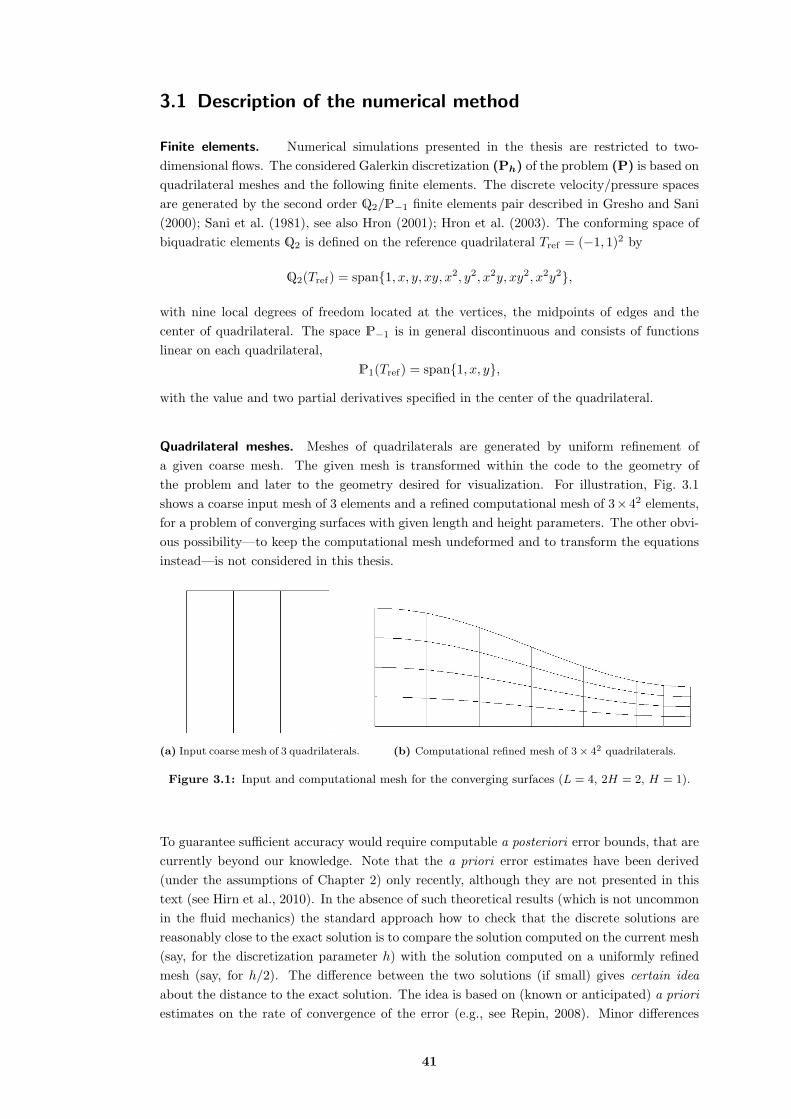
3.1 Description of the numerical method

Finite elements. Numerical simulations presented in the thesis are restricted to two-dimensional flows. The considered Galerkin discretization (Ph) of the problem (P) is based onquadrilateral meshes and the following finite elements. The discrete velocity/pressure spacesare generated by the second order Q2/P−1 finite elements pair described in Gresho and Sani(2000); Sani et al. (1981), see also Hron (2001); Hron et al. (2003). The conforming space ofbiquadratic elements Q2 is defined on the reference quadrilateral Tref = (−1, 1)2 by

Q2(Tref) = span1, x, y, xy, x2, y2, x2y, xy2, x2y2,

with nine local degrees of freedom located at the vertices, the midpoints of edges and thecenter of quadrilateral. The space P−1 is in general discontinuous and consists of functionslinear on each quadrilateral,

P1(Tref) = span1, x, y,

with the value and two partial derivatives specified in the center of the quadrilateral.

Quadrilateral meshes. Meshes of quadrilaterals are generated by uniform refinement ofa given coarse mesh. The given mesh is transformed within the code to the geometry ofthe problem and later to the geometry desired for visualization. For illustration, Fig. 3.1shows a coarse input mesh of 3 elements and a refined computational mesh of 3×42 elements,for a problem of converging surfaces with given length and height parameters. The other obvi-ous possibility—to keep the computational mesh undeformed and to transform the equationsinstead—is not considered in this thesis.

(a) Input coarse mesh of 3 quadrilaterals. (b) Computational refined mesh of 3× 42 quadrilaterals.

Figure 3.1: Input and computational mesh for the converging surfaces (L = 4, 2H = 2, H = 1).

To guarantee sufficient accuracy would require computable a posteriori error bounds, that arecurrently beyond our knowledge. Note that the a priori error estimates have been derived(under the assumptions of Chapter 2) only recently, although they are not presented in thistext (see Hirn et al., 2010). In the absence of such theoretical results (which is not uncommonin the fluid mechanics) the standard approach how to check that the discrete solutions arereasonably close to the exact solution is to compare the solution computed on the current mesh(say, for the discretization parameter h) with the solution computed on a uniformly refinedmesh (say, for h/2). The difference between the two solutions (if small) gives certain ideaabout the distance to the exact solution. The idea is based on (known or anticipated) a prioriestimates on the rate of convergence of the error (e.g., see Repin, 2008). Minor differences

41

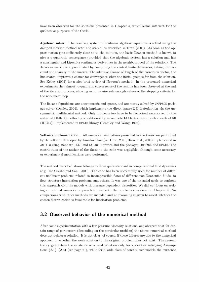
have been observed for the solutions presented in Chapter 4, which seems sufficient for thequalitative purposes of the thesis.

Algebraic solver. The resulting system of nonlinear algebraic equations is solved using thedamped Newton method with line search, as described in Hron (2001). As soon as the ap-proximation gets sufficiently close to to the solution, the basic Newton method is known togive a q-quadratic convergence (provided that the algebraic system has a solution and hasa nonsingular and Lipschitz continuous derivatives in the neighbourhood of the solution). TheJacobian matrix is approximated by computing the central finite differences, taking into ac-count the sparsity of the matrix. The adaptive change of length of the correction vector, theline search, improves a chance for convergence when the initial guess is far from the solution.See Kelley (2003) for a nice brief review of Newton’s method. In the presented numericalexperiments the (almost) q-quadratic convergence of the residua has been observed at the endof the iteration process, allowing us to require safe enough values of the stopping criteria forthe non-linear loop.

The linear subproblems are unsymmetric and sparse, and are mostly solved by UMFPACK pack-age solver (Davies, 2004), which implements the direct sparse LU factorization via the un-symmetric multifrontal method. Only problems too large to be factorized were solved by therestarted GMRES method preconditioned by incomplete LU factorization with s levels of fill(ILU(s)), implemented in SPLIB library (Bramley and Wang, 1995).

Software implementation. All numerical simulations presented in the thesis are performedby the software developed by Jaroslav Hron (see Hron, 2001; Hron et al., 2003) implemented inANSI C using standard BLAS and LAPACK libraries and the packages UMFPACK and SPLIB. Thecontribution of the author of the thesis to the code was negligible, although some necessaryor experimental modifications were performed.

The method described above belongs to those quite standard in computational fluid dynamics(e.g., see Gresho and Sani, 2000). The code has been successfully used for number of differ-ent nonlinear problems related to incompressible flows of different non-Newtonian fluids, toflow–structure interaction problems and others. It was one of the intended goals to confrontthis approach with the models with pressure dependent viscosities. We did not focus on seek-ing an optimal numerical approach to deal with the problems considered in Chapter 4. Nocomparisons with other methods are included and no reasoning is given to assert whether thechosen discretization is favourable for lubrication problems.

3.2 Observed behavior of the numerical method

After some experimentation with a few pressure–viscosity relations, one observes that for cer-tain range of parameters (depending on the particular problem) the above numerical methoddoes not deliver a solution. It is not clear, of course, if these failures are due to the numericalapproach or whether the weak solution to the original problem does not exist. The presenttheory guarantees the existence of a weak solution only for viscosities satisfying Assump-tions (A1)–(A3) (see page 21), while for a wide class of constitutive models the existence

42

is an open problem. The assumptions (A2)–(A3) are not needed to prove the existence ofdiscrete solutions (see Theorem 11) but they are required to show its uniqueness.

It was an original intention of the author to verify whether the models satisfying (A1)–(A3)allow for a robust numerical treatment and whether they can be used to approximate lubri-cants in real-world applications. We illustrate in Chapter 5 that such models can approximatethe real-world liquids only in a restricted range of parameters. However, the numerical exper-iments show that we obtain the discrete solutions for a set of problems larger than given by(A1)–(A3). In fact, the author did observed no obvious change of behavior of the numericalmethod and no qualitative change of solutions, which could be linked to the violation of theseassumptions. This indicates that (A1)–(A3) are related to the technique of the proofs, andthat Problem (P) may be well-posed for a wider class of viscosity models.

In the following, we report on the numerical experiments suggesting that the condition deter-mining the convergence of the considered numerical method to the discrete solution is (A4).We show in Chapter 5 that this allows to model real liquids over significantly broader rangeof parameters, see Section 5.3.

3.3 Condition (A4) seems to determine the numerical

stability

To illustrate the point, we examine the flow between converging plates, which is described indetail in Section 4.2. The viscosity (1.12) of the three reference liquids from Subsection 1.3.4will be used. The flow is induced solely by the tangential motion of the lower surface, anda pressure peak is generated in the middle left part of the domain due to the converginggeometry. The height of the domain will be fixed, H = 10−5 m at the output and 2H atthe input. We will play with two parameters: the length of the considered domain, L, andthe velocity of the lower surface, V . Note that the velocity profile is approximately linear atthe cross-section concurrent with the pressure peak location, and that the values of |D(vvv)|are then approximately of the order V/H. By increasing L, the resulting pressure values areincreased, while by increasing V , both the values of |D(vvv)| and p are increased. Examples ofthe resulting flow are presented in detail in Section 4.2.

Here we proceed as follows: for different liquids, by taking different L and V we arrange forsolutions with different values of |D(vvv)|. Then, we increase V as long as the method convergesto a discrete solution; the solution obtained for current V is always taken as the initial guessfor the next problem. After certain limit is reached, the Newton method does not convergeany more, not even if the next V is taken very close to the previous one (so that the initialresidual is very small). What happens is either that the Jacobian matrix becomes singular,or the nonlinear iterations diverge until the represented variables become infinite in computerarithmetic.

Table 3.1 shows a set of experiments with different liquids. We report the values of L, levelsof mesh refinement, and three values of V : For the third value of V , the method does notconverge any more; the second value of V is the “critical” value, while the first value is onlya “sub-critical” example. For illustration, Figure 3.2 depicts the solution of the last experimentof the table for V = 31.84 m.

43

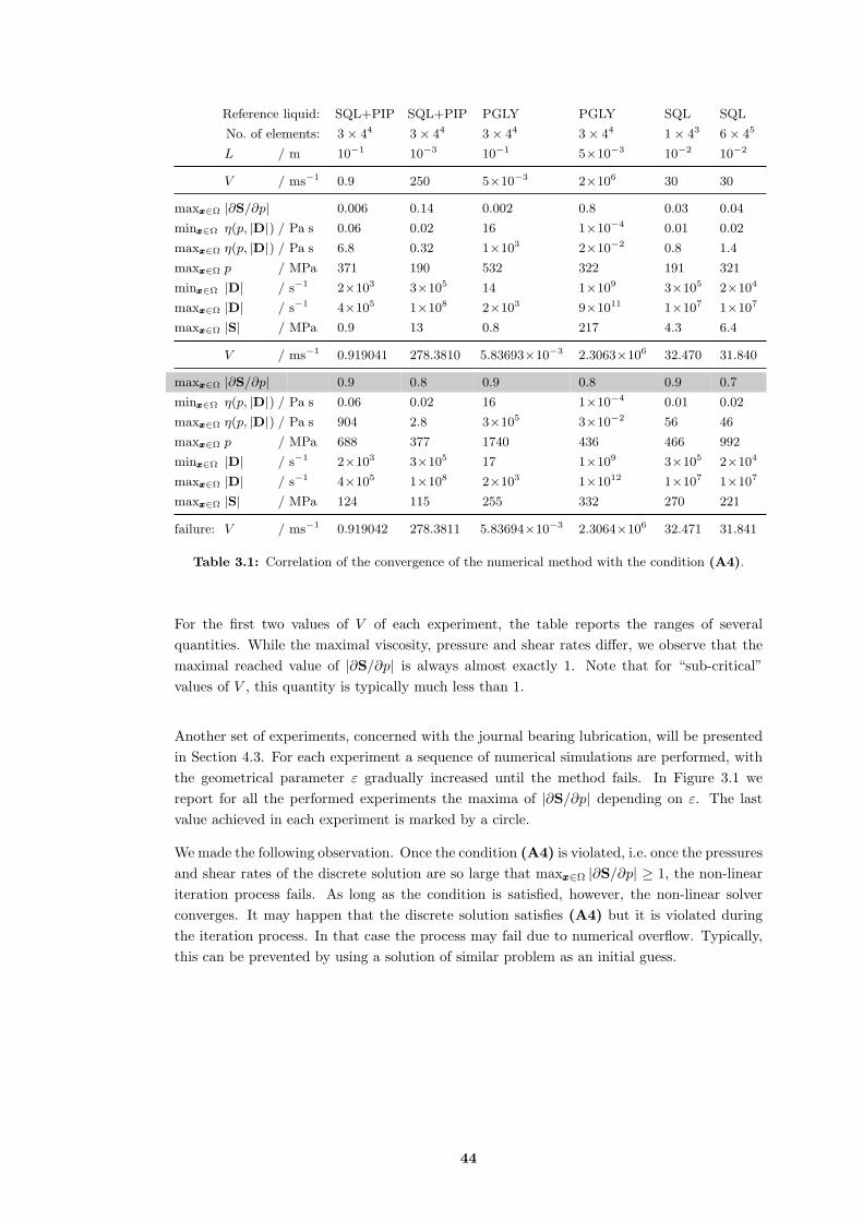
Reference liquid: SQL+PIP SQL+PIP PGLY PGLY SQL SQL

No. of elements: 3× 44 3× 44 3× 44 3× 44 1× 43 6× 45

L / m 10−1 10−3 10−1 5×10−3 10−2 10−2

V / ms−1 0.9 250 5×10−3 2×106 30 30

maxxxx∈Ω |∂S/∂p| 0.006 0.14 0.002 0.8 0.03 0.04

minxxx∈Ω η(p, |D|) / Pa s 0.06 0.02 16 1×10−4 0.01 0.02

maxxxx∈Ω η(p, |D|) / Pa s 6.8 0.32 1×103 2×10−2 0.8 1.4

maxxxx∈Ω p / MPa 371 190 532 322 191 321

minxxx∈Ω |D| / s−1 2×103 3×105 14 1×109 3×105 2×104

maxxxx∈Ω |D| / s−1 4×105 1×108 2×103 9×1011 1×107 1×107

maxxxx∈Ω |S| / MPa 0.9 13 0.8 217 4.3 6.4

V / ms−1 0.919041 278.3810 5.83693×10−3 2.3063×106 32.470 31.840

maxxxx∈Ω |∂S/∂p| 0.9 0.8 0.9 0.8 0.9 0.7

minxxx∈Ω η(p, |D|) / Pa s 0.06 0.02 16 1×10−4 0.01 0.02

maxxxx∈Ω η(p, |D|) / Pa s 904 2.8 3×105 3×10−2 56 46

maxxxx∈Ω p / MPa 688 377 1740 436 466 992

minxxx∈Ω |D| / s−1 2×103 3×105 17 1×109 3×105 2×104

maxxxx∈Ω |D| / s−1 4×105 1×108 2×103 1×1012 1×107 1×107

maxxxx∈Ω |S| / MPa 124 115 255 332 270 221

failure: V / ms−1 0.919042 278.3811 5.83694×10−3 2.3064×106 32.471 31.841

Table 3.1: Correlation of the convergence of the numerical method with the condition (A4).

For the first two values of V of each experiment, the table reports the ranges of severalquantities. While the maximal viscosity, pressure and shear rates differ, we observe that themaximal reached value of |∂S/∂p| is always almost exactly 1. Note that for “sub-critical”values of V , this quantity is typically much less than 1.

Another set of experiments, concerned with the journal bearing lubrication, will be presentedin Section 4.3. For each experiment a sequence of numerical simulations are performed, withthe geometrical parameter ε gradually increased until the method fails. In Figure 3.1 wereport for all the performed experiments the maxima of |∂S/∂p| depending on ε. The lastvalue achieved in each experiment is marked by a circle.

We made the following observation. Once the condition (A4) is violated, i.e. once the pressuresand shear rates of the discrete solution are so large that maxxxx∈Ω |∂S/∂p| ≥ 1, the non-lineariteration process fails. As long as the condition is satisfied, however, the non-linear solverconverges. It may happen that the discrete solution satisfies (A4) but it is violated duringthe iteration process. In that case the process may fail due to numerical overflow. Typically,this can be prevented by using a solution of similar problem as an initial guess.

44

(a)p

(b)|D

(vv v)|

(logari

thm

ic)

(c)η(p,|D

(vv v)|

)(l

ogari

thm

ic)

(d)|S

(p,D

(vv v))|

(logari

thm

ic)

(e)vv v·ee ex

(f)vv v·ee ey

(g)

the

stre

am

lin

es(h

)|∂

S/∂p|

(logari

thm

ic)

Fig

ure

3.2

:E

xam

ple

solu

tion

close

toth

elim

its

of

the

num

eric

al

met

hod.

45

0.7 0.75 0.8 0.85 0.9 0.95 110

−4

10−3

10−2

10−1

100

101

relative eccentricity, ε

max

imal

rea

ched

|dS

/dp|

Figure 3.3: maxxxx∈Ω |∂S/∂p| depending on ε for all experiments presented in Section 4.3.

46

Chapter 4

Numerical simulations

Contents

4.1 Planar Poiseuille flow . . . . . . . . . . . . . . . . . . . . . . . 48

4.2 Sliding converging surfaces . . . . . . . . . . . . . . . . . . . . 49

4.2.1 Flow with pressure-thickening and shear-thinning lubricant . . . . 50

4.2.2 Sensitivity of the pressure field due to pressure-thickening . . . . . 55

4.3 Planar steady flow in journal bearing . . . . . . . . . . . . . . . 56

4.3.1 Basic features of the flow . . . . . . . . . . . . . . . . . . . . . . 58

4.3.2 Exact solution for the constant viscosity lubricant flow . . . . . . 58

4.3.3 The influence of shear-thinning and pressure-thickening . . . . . 60

4.3.4 Importance of the level of pressure . . . . . . . . . . . . . . . . . 67

47

4.1 Planar Poiseuille flow

Consider the classical example of the flow in between infinite parallel plates (say, y = 0 andy = H > 0), where everything is uniform with the z-coordinate and the flow is planar in thex, y-plane. Assume no-slip conditions at the plates which are held steady, i.e., set vvv = 000 at theplates. For a Newtonian fluid, as well as for non-Newtonian fluids with the viscosity dependingonly on the shear rate, there exists a unidirectional Poiseuille flow driven by a constant pressuregradient

η = η(|D|), vvv = (u(y), 0), p = p(x) = Gpx, (4.1)

where Gp ∈ R and the velocity profile are related by

Gp = u′′(y)η( |u′(y)|√

2

)+ η′

( |u′(y)|√2

) |u′(y)|√2

.

The situation is more complex for the piezoviscous fluid, however. As was shown by Bairet al. (1998) and confirmed rigorously by Hron et al. (2011, 2001), e.g. for the Barus modelη = η0 exp(αp) the unidirectional flow does not exist. A pressure gradient across the fluid filmand a corresponding secondary flow has to be expected, which has however not been reachedby analytical methods.

The following numerical simulation aims to show the behavior of the flow between stationaryparallel plates. Naturally, we have to restrict ourselves to a finite domain, where the flow isinduced by the pressure drop between inflow and outflow. Let us comment on the boundaryconditions at the artificial boundaries x = 0 and x = L > 0. Note that the condition (1.20)

−Tnnn = P (x)

is not a good choice as long as concerns this kind of flow (in straight channels). This can beillustrated by the example (4.1), where one observes (for nnn = eeex) that

−Tnnn =(p(x) , η

( |u′(y)|√2

)u′(y)

).

Note that the second component of the right hand side is not constant across the fluid filmand, more importantly, it includes the complete information about the velocity profile. Bysetting (1.20) with bbb = (P (x), 0), the resulting flow would not be unidirectional (see Heywoodet al., 1996).

Here, due to our concern with simple (unidirectional) flows, we set the condition (1.21)

vvvτττ = 000 and −Tnnn ·nnn = P (x), (4.2)

i.e., we enforce the flow parallel to the plates at the boundary (vvv ·eeey = 0), while we determinethe pressure values by prescribing the normal part of the traction.

In the following example, we take the Barus viscosity model η = η0 exp(αp) with the param-eters

η0 = 16.3 Pa s , α = 1.3×10−8 Pa−1,

48

(it approximates the PGLY reference liquid at T = 40 C if the shear-thinning is ignored, seeSubsection 1.3.4). Moreover, merely in order to separate the interesting features of the flowfrom the (unknown) influence of the artificial boundary condition at the inflow, we cut off theviscosity above certain value; this results into a unidirectional flow near the inflow boundary.To summarize, we take the following setting:

η = η0 exp(αp), where p = minp, 150 MPaP (0) = 300 MPa, P (L) = 0, L = 3×10−5 m, H = 1×10−5 m.

The resulting flow is reported in Figure 4.1. In the left part near the inflow, where the pressureis above the cut-off and the viscosity is constant, we observe the unidirectional Poiseuille flowwith the pressures constant across the film; in the middle and right part, the effect of thepiezoviscous viscosity is visible: The pressure gradient is no more parallel to the plates anda secondary flow occures. Note that we would observe analogous flows even without the cut-off; also note that the fluids with both pressure-thickening and shear-thinning viscosity wouldgive analogous results in this example.

(a) the pressure p (b) the viscosity η(p)

(c) the velocity component vvv ·eeex (d) the velocity component vvv ·eeey

Figure 4.1: The flow of a piezoviscous fluid between parallel plates.

4.2 Sliding converging surfaces

The simple flows in straight channels or between parallel plates are lacking the most essentialfeature of hydrodynamic lubrication: the pressure peak generated by the flow, which allows tocarry high loads. The simple problem which allows to study this feature is the flow betweenplates whose distance decreases in the direction of the flow.

We will study the following problem: everything is uniform in the z-coordinate and a planarflow is studied in the x, y-plane. The lower plate is defined by y = 0, the upper is describedby y = h(x) > 0. We restrict our attention to the interval x ∈ (0, L) and we set h(x) =H( 3

2 + 12 cos(xπ/L)); this is chosen so that h(0) = 2H, h(L) = H and h′(0) = h′(L) = 0, see

Figure 4.2. In this study, we always set H = 10−5 m.

We concentrate on sliding conditions: the upper plate is considered steady, while the lowermoves with the velocity V . These are more relevant to journal bearing lubrication than, for

49

vvv = V eeex

vvv = 000

L

2H

Hvvv · eeey = 0

−Teeex · eeex = Pout

vvv · eeey = 0

−Teeex · eeex = Pin

Figure 4.2: The geometry of converging surfaces problem.

example, rolling conditions where the upper plate would progress (tangentially) in the samedirection as the lower plate, and the resulting flow would be of a different type. On thesurfaces we will assume no-slip conditions, i.e. we set vvv = vvvτττ = V eeex on the lower and vvv = 000on the upper boundary. On the artificial inflow and outflow boundaries we set the boundarycondition (1.21), i.e., we prescribe that the flow through the boundaries is parallel to the lowerplate and we determine the inflow and outflow pressures.

4.2.1 Flow with pressure-thickening and shear-thinning lubricant

We report numerical solutions to the following four examples with the reference liquids fromSubsection 1.3.4.

i) SQL, L = 3×10−3 m, V = 102 m/s, Figure 4.3;

ii) PGLY, L = 5×10−3 m, V = 101 m/s, Figure 4.4;

iii) SQL+PIP, L = 10−2 m, V = 101 m/s, Figure 4.5;

iv) SQL+PIP, L = 10−3 m, V = 102 m/s, Figure 4.6.

In all the examples, H = 10−5 m, and zero normal component of traction (4.2) is given atboth the inflow and outflow boundaries, P (0) = P (L) = 0. The parameters chosen in theexamples above do not follow any particular scheme, and analogous results could be achievedby using any one of the reference liquids.

In the SQL example, the viscosity field is clearly dominated by pressure-thickening and is,same as the pressure field, almost constant across the fluid film. In all the other examplesboth shear-thinning and pressure-thickening are significant, displaying two local maxima inthe viscosity field: one due to the pressure peak, one due to the local minimum of shearrate which occurs at the point of bifurcation of the flow and extends upstream through thebackward flow whirl. The resulting viscosity field then shows slightly different shapes in thethree examples: the sharp and long ridge in Figure 4.6 following the narrow of the shear rateminimum; the round jutting more connected to the pressure peak area in Figure 4.5; or thewell localized maximum adherent to the upper plate in the PGLY example in Figure 4.4.

The examples demonstrate that the viscosity cannot be considered constant across the fluidfilm once the shear-thinning takes place. Once the backward flow appears, a sharp minimumof the shear rates emerges which can affect the viscosity significantly.

The selected examples, however, show no surprising results. In particular, no secondary flowrelated solely to the pressure-thickening manifested within the range of parameters allowed

50

(a)p

(b)|D

(vv v)|

(logari

thm

ic)

(c)η(p,|D

(vv v)|

)(d

)|D

(vv v)|

(e)

the

stre

am

lin

es(f

)|S

(p,D

(vv v))|

(g)vv v·ee ex

(h)vv v·ee ey

Fig

ure

4.3

:E

xam

ple

flow

bet

wee

nco

nver

gin

gpla

tes,

SQ

L,L

=3×

10−

3m

,V

=10

2m/s.

51

(a)p

(b)|D

(vv v)|

(logari

thm

ic)

(c)η(p,|D

(vv v)|

)(d

)|D

(vv v)|

(e)

the

stre

am

lin

es(f

)|S

(p,D

(vv v))|

(g)vv v·ee ex

(h)vv v·ee ey

Fig

ure

4.4

:E

xam

ple

flow

bet

wee

nco

nver

gin

gpla

tes,

PG

LY

,L

=5×

10−

3m

,V

=10

1m/s.

52

(a)p

(b)|D

(vv v)|

(logari

thm

ic)

(c)η(p,|D

(vv v)|

)(d

)|D

(vv v)|

(e)

the

stre

am

lin

es(f

)|S

(p,D

(vv v))|

(g)vv v·ee ex

(h)vv v·ee ey

Fig

ure

4.5

:E

xam

ple

flow

bet

wee

nco

nver

gin

gpla

tes,

SQ

L+

PIP

,L

=10−

2m

,V

=10

1m/s.

53

(a)p

(b)|D

(vv v)|

(logari

thm

ic)

(c)η(p,|D

(vv v)|

)(d

)|D

(vv v)|

(e)

the

stre

am

lin

es(f

)|S

(p,D

(vv v))|

(g)vv v·ee ex

(h)vv v·ee ey

Fig

ure

4.6

:E

xam

ple

flow

bet

wee

nco

nver

gin

gpla

tes,

SQ

L+

PIP

,L

=10−

3m

,V

=10

2m/s.

54

by the numerical method. The features observed in the examples ii)–iv) are related to theinterplay between shear-thinning and pressure-thickening.

4.2.2 Sensitivity of the pressure field due to pressure-thickening

As shown by the preceding examples, the pressure field is virtually constant across the fluidfilm; thus, we can draw the pressure profiles of the resulting flow along the x-coordinate. Inthis subsection, we report on a feature specific to flows of pressure-thickening fluids. Thepressure peak can display a significant sensitivity on the pressure values far from the area ofinterest.

This is a known fact, which however should be emphasized for its several consequences: Theresulting flow can depend severely on the values prescribed at the inflow/outflow boundaries(or, in other words, on the resulting level of the pressure). Moreover, considering the errordue to discretization and the numerical approximation, one should keep in mind that the errorallowed at one place may possibly be magnified while carried to the other part of the domain.Further, one can expect that the properties of the numerical problems to be solved, such asthe performance of the non-linear solver, the conditioning of the linear subproblems or, e.g.,the requirements on their successful preconditioning, may be different compared to problemswhere the viscosity does not depend on pressure.

0 0.5 1 1.5 2 2.5 3

x 10−3

0

0.5

1

1.5

2

2.5

3

3.5

4

4.5

5x 10

8

x coordinate / [m]

pres

sure

/ [P

a]

(a) Pressure profiles with P (0) = 0 (full line),1 MPa (dash) and 10 MPa (dash dotted) and withP (L) = 0.

0 0.5 1 1.5 2 2.5 3

x 10−3

0

1

2

3

4

5

6

7

8

9x 10

8

x coordinate / [m]

pres

sure

/ [P

a]

(b) Pressure profiles with P (0) = P (L) = 0 (fullline), 1 MPa (dash) and 10 MPa (dash dotted).

Figure 4.7: Pressure profiles for SQL, L = 3×10−3 m, V = 102 m/s.

We illustrate the issue by the following simple observations based on the example i) of theprevious subsection. In Figure 4.7a we increase the traction prescribed at the inflow fromP (0) = 0 to P (0) = 1 MPa and 10 MPa; in Figure 4.7b both P (0) and P (L) are increasedanalogously. Note that since the viscosity depends on pressure approximately exponentially,the sensitivity of the pressure peak on the boundary values is the more intense the higher isthe pressure peak, and can be much less or much more intense than in Figure 4.7.

55

4.3 Planar steady flow in journal bearing

In this section we will examine the basic features of the flow of lubricant in a simple modelof journal bearing. Let us recall what was briefly introduced in Subsection 1.1.1 and specifythe setting for our numerical experiments in more detail. The journal and the bearing aresolid cylinders with parallel eccentric axes, the outer (bearing) is held steady while the inner(journal) rotates about its own axis. The lubricant is introduced between the solid surfacesand its flow is induced by the journal rotation. In hydrodynamic regime the solid surfaces arewell separated by the fluid film.

It is not our ambition to approach the full complexity of the problem nor to give particularengineering predictions; our aim is merely to pinpoint some features related to the constitutivemodel. For clarity of exposition and in order to reduce the amount of model parameters, wetake several simplifications: the solid cylinders are rigid; the space between them is filledby the fluid entirely (full-film conditions); the fluid is incompressible and is able to sustainarbitrary negative pressures; inertial forces are neglected; no-slip conditions are considered atthe solid surfaces.

e

RJ

RB

ω

φ

Figure 4.8

RJ 3.125×10−2 m

RB 3.129×10−2 m

Table 4.1

Planar flow. We take the long bearing approximation, consideringonly a planar flow, uniform in the direction of cylinders axes; inother words, we study a two-dimensional flow in an eccentric an-nulus. The geometry is depicted on Figure 4.8 and is described bythree parameters, the radii RJ < RB and the relative eccentricityε ∈ 〈0, 1) defined by ε(RB − RJ) = e, where e is the distance be-tween the journal and bearing axes. Throughout this section, wetake the geometrical parameters given by Table 4.1 that were usedin a series of papersa by Davies, Gwynllyw, Li and Phillips.

Steady flow. We confine ourselves to studying steady flows in fixedgeometry, i.e., in the geometry with the relative eccentricity ε pre-scribed as an input parameter. With the steady solutions, we willbe interested in the maxima and the distribution of several quanti-ties within the flow field, and in the resulting force exerted on thejournal by the fluid, defined by

FFF =ˆ

ΓJ

(−Tnnn) dxxx,

where ΓJ denotes the journal surface and nnn the unit outward normal vector. In real world,the rotating journal (when working in hydrodynamic regime) ”floats” in the lubricant, beingactuated by the resultant of applied load and of the forces due to the lubricant flow. Assumingthat the motion of the journal axis is slow compared to the rotation speed, one can interpretthe steady flow problem as a quasi-steady approximation to the unsteady flow at certain timeand position of the journal axis. In particular, if the applied load is constant in time, thejournal axis can eventually reach a steady state, where the applied load is in balance with theforce FFF exerted by the fluid. Note that such a stable equilibrium may or may not be reached;for example, it is well-documented in the literature (e.g., see Brindley et al. (1983); Li et al.(2000b)) that under the assumptions of full-film and constant viscosity lubricant, the journal

a See Gwynllyw et al. (1996a,b); Gwynllyw and Phillips (1996, 2005); Li et al. (2000a, 1999, 2000b)

56

exhibits a half-speed whirl: the trajectory of the journal spirals towards the bearing whilethe angular velocity of its path approaches ω/2, where ω denotes the angular velocity of thejournal rotation. On the other hand, the steady equilibria can be reached if cavitation and/orpressure-dependent viscosity is present in the model, see Gwynllyw et al. (1996b). We will notaddress the very interesting questions of dynamical behavior of the journal bearing system.

Problem setting. To summarize, we perform the following numerical experiments concernedwith Problem (Ph). Gravity is neglected, fff = 000, and since the convective term is not con-sidered either, the density of the lubricant does not appear in the governing equations. Thedomain is an eccentric annulus with the parameters given by Table 4.1 and with the relativeeccentricity ε ∈ 〈0, 1) given later. The viscosity models for the three reference lubricantsdescribed in Subsection 1.3.4 will be considered, always at the temperature T = 100 C. Atnegative pressures, we simply extend these models by defining

η(p, |D|) :=

if p ≥ 0, η(p, |D|),if p < 0, ηmin(|D|) + (η(0, |D|)− ηmin(|D|)) exp

(∂pη(p,|D|)|p=0

η(0,|D|)−ηmin(|D|) p)

where ηmin(|D|) := min10−3η(0, 0), 12η(0, |D|). On the entire boundary, the Dirichlet

boundary conditions are prescribed, namely vvv = 000 on the outer circle and vvv = (ωRJ)τττ onthe inner circle, where τττ is a clock-wise unit tangential vector and where ω is specified as fol-lows: for SQL and SQL+PIP we set ω = 103 rad/s, while for PGLY we choose ω = 10 rad/s.The condition required to fix the level of pressure will be discussed.

(a) Input coarse meshof 1× 6 quadrilaterals.

(b) Mesh of 21 × 6 · 21 elements,RJ = 0.5, ε = 0.5.

(c) Mesh of 22 × 6 · 22 elements,RJ = 0.8, ε = 0.8.

Figure 4.9: Input and transformed meshes for the journal bearing problem (RB = 1).

Similarly as described in Subsection 3.1, the computational mesh of quadrilaterals is producedby geometrical transformation of the input coarse mesh, which has a simple concentric geom-etry. We will not specify this transformation in detail, see the example in Figure 4.9; notethat while the geometrical deformation is linear in the radial direction, in the angular direc-tion it is chosen such that the local ratio between the angular and radial lengths is preservedthroughout the domain. The figures of the flow domain in this section use the same kind oftransformation, usually with the radii 0.5 and 1 and the eccentricity ε = 0.5.

In all the numerical experiments presented, the computational mesh consists of 24 × 128 · 24

quadrilaterals (2n refers to n uniform refinements). This seems sufficient for our purposes(which are basically qualitative), the differences observed when compared to a solution at thecoarser mesh have been minor.

57

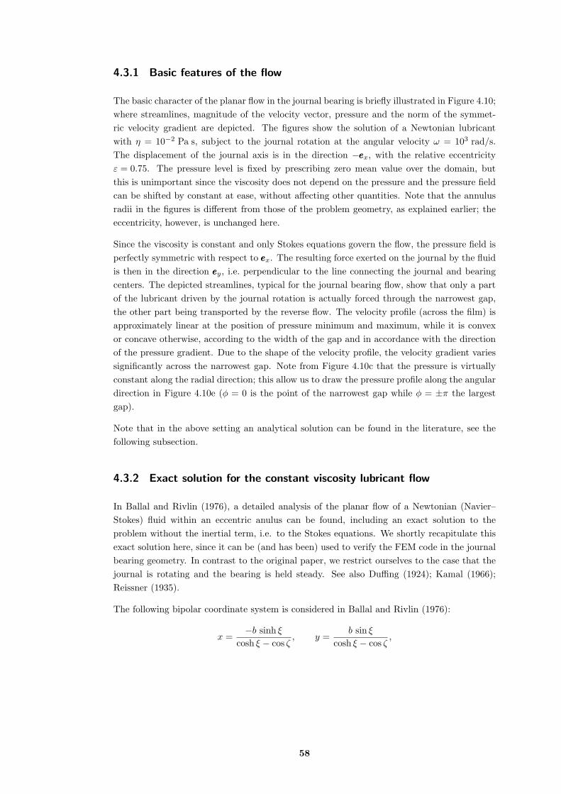
4.3.1 Basic features of the flow

The basic character of the planar flow in the journal bearing is briefly illustrated in Figure 4.10;where streamlines, magnitude of the velocity vector, pressure and the norm of the symmet-ric velocity gradient are depicted. The figures show the solution of a Newtonian lubricantwith η = 10−2 Pa s, subject to the journal rotation at the angular velocity ω = 103 rad/s.The displacement of the journal axis is in the direction −eeex, with the relative eccentricityε = 0.75. The pressure level is fixed by prescribing zero mean value over the domain, butthis is unimportant since the viscosity does not depend on the pressure and the pressure fieldcan be shifted by constant at ease, without affecting other quantities. Note that the annulusradii in the figures is different from those of the problem geometry, as explained earlier; theeccentricity, however, is unchanged here.

Since the viscosity is constant and only Stokes equations govern the flow, the pressure field isperfectly symmetric with respect to eeex. The resulting force exerted on the journal by the fluidis then in the direction eeey, i.e. perpendicular to the line connecting the journal and bearingcenters. The depicted streamlines, typical for the journal bearing flow, show that only a partof the lubricant driven by the journal rotation is actually forced through the narrowest gap,the other part being transported by the reverse flow. The velocity profile (across the film) isapproximately linear at the position of pressure minimum and maximum, while it is convexor concave otherwise, according to the width of the gap and in accordance with the directionof the pressure gradient. Due to the shape of the velocity profile, the velocity gradient variessignificantly across the narrowest gap. Note from Figure 4.10c that the pressure is virtuallyconstant along the radial direction; this allow us to draw the pressure profile along the angulardirection in Figure 4.10e (φ = 0 is the point of the narrowest gap while φ = ±π the largestgap).

Note that in the above setting an analytical solution can be found in the literature, see thefollowing subsection.

4.3.2 Exact solution for the constant viscosity lubricant flow

In Ballal and Rivlin (1976), a detailed analysis of the planar flow of a Newtonian (Navier–Stokes) fluid within an eccentric anulus can be found, including an exact solution to theproblem without the inertial term, i.e. to the Stokes equations. We shortly recapitulate thisexact solution here, since it can be (and has been) used to verify the FEM code in the journalbearing geometry. In contrast to the original paper, we restrict ourselves to the case that thejournal is rotating and the bearing is held steady. See also Duffing (1924); Kamal (1966);Reissner (1935).

The following bipolar coordinate system is considered in Ballal and Rivlin (1976):

x =−b sinh ξ

cosh ξ − cos ζ, y =

b sin ξcosh ξ − cos ζ

,

58

(a) streamlines (b) |vvv|

(c) p (d) |D(vvv)|

−1 −0.8 −0.6 −0.4 −0.2 0 0.2 0.4 0.6 0.8 1−6

−4

−2

0

2

4

6x 10

7

angular coordinate φ / π [rad]

pres

sure

/ [P

a]

(e) p

Figure 4.10: Basic features of the flow in journal bearing, ε = 0.75, ω = 103 rad/s, η = 10−2 Pa s.

59

where ξ ∈ (ξJ , ξB) and ζ ∈ (0, 2π) and where

b =12e[(R2

B +R2J − e2)2 − 4R2

BR2J

] 12 ,

sinh ξB = − b

RB,

sinh ξJ = − b

RJ.

The resulting pressure field is given by (P0 being an arbitrary constant, µ denotes the constantviscosity)

p = P0 +2µωRJ

b[q1(ξ) sin ζ + q2(ξ) sin 2ζ] , (4.3)

where

q1(ξ) = (f8 − 2f10) sinh ξ − 2f12 cosh ξ,

q2(ξ) = f10 sinh 2ξ + f12 cosh 2ξ,

f8 = − sinh2(ξB − ξJ) sinh ξB /∆∗,

f10 = −h2 sinh(ξB + ξJ) /(2∆∗),

f12 = h2 cosh(ξB + ξJ) /(2∆∗),

∆∗ = sinh(ξB − ξJ)[2 sinh ξB sinh ξJ sinh(ξB − ξJ)

− (ξB − ξJ)(sinh2 ξB + sinh2 ξJ)]< 0,

h2 = −(ξB − ξJ) sinh ξJ + sinh ξB sinh(ξB − ξJ) > 0.

For the velocity field, see Ballal and Rivlin (1976, (4.1) on p. 242). The reaction force FFF =(0, Fy) and the moment M of the forces acting on the unit length of the journal are given by

Fy = 2µωR2J

RBF , (4.4)

M = 2µω(R2JM +R2

BM), (4.5)

where

F = − 2π∆∗

sinh ξJ sinh2(ξB − ξJ) < 0,

M =2π∆∗

sinh3(ξB − ξJ) < 0,

M =2π∆∆∗

sinh2(ξB) < 0,

∆ = (ξB − ξJ) cosh(ξB − ξJ)− sinh(ξB − ξJ) > 0.

4.3.3 The influence of shear-thinning and pressure-thickening

We compute the steady flows for a sequence of relative eccentricities (we proceed by a naturalparameter continuation: ε is gradually increased, taking the previous solution as an initialguess, while the next ε is chosen such that the algebraic residuum of the initial guess isbelow a given bound). Eventually, for some ε large enough, the resulting pressures and shearrates within the actual approximation are such that the condition (A4) is violated, and the

60

nonlinear algebraic solver fails as described in Section 3.2. Otherwise (i.e., for experimentswhere the viscosity does not depend on pressure, so that (A4) holds trivially), we stop thesequence at ε = 0.99. The pressure level is fixed by prescribing zero pressure at the point ofthe largest gap φ = π (see the next subsection for details).

We examine the following four variants of the three experiments:

i) the original reference viscosity model, η := η(p, |D(vvv)|), full lines;

ii) the shear-thinning model, η := η(0, |D(vvv)|), dash lines;

iii) the pressure-thickening model, η := η(p, D), dash dotted lines;here D

√2 = ωRJ/(RB − RJ), which yields D = 5.5×105 s−1 for SQL and SQL+PIP,

and D = 5.5×103 s−1 for PGLY;

iv) the constant viscosity model, η := η(0, D), dotted lines.

liquid SQL PGLY SQL+PIPangular velocity ω 103 rad/s 10 rad/s 103 rad/sapplied load |FFF | 2×106 N/m 1×107 N/m 4×106 N/m

i) reference model 0.925 0.80 0.80ii) shear-thinning 0.972 0.92 0.89

iii) pressure-thickening 0.925 0.76 0.75iv) constant viscosity 0.972 0.91 0.84

Table 4.2: Relative eccentricities corresponding to given applied load,influence of non-Newtonian viscosity.

In Figures 4.11 and 4.12, we report the resulting dependence of |FFF | and of the angle Fφ :=∠(FFF ,−eeex) on the relative eccentricity ε. In Table 4.2 we choose an example of applied loadfor each liquid, and we report the corresponding eccentricity at which the balanced positionof the journal may be observed. Figures 4.13 and 4.14 depicts the maximum reached valuesof pressure, and the maximum and minimum values of viscosity.

The figures and the table are quite self-explanatory and the results are not surprising. Theinfluence of the pressure-thickening is substantial in all examples. For SQL, no effects relatedto the shear-thinning are visible, since this liquid does not exhibit shear-thinning unless forhigher shear rates. For the other liquids, however, its influence is significant, whether ornot the pressure-thickening is also present in the model. Note from Figure 4.12 that whenthe viscosity does not vary with pressure, then Fφ = π/2, i.e. the vector of exerted force isexactly perpendicular to the line connecting the cylinders axes; the dependence of the viscosityon pressure changes this behavior dramatically. (It should be mentioned that the presenceof cavitation would have analogous effect.) Note that the maximal pressures we are able toapproach with the numerical simulations are reaching 1 GPa for SQL and SQL+PIP, and even3 GPa for PGLY lubricant examples; cf. Section 5.3 and Figure 5.10.

Figures 4.15–4.19 illustrate how the viscosity which depends both on pressure and shear ratevaries. In the presented examples, the variation of the viscosity across the fluid film appearsdue to the dependence on the shear rate. For PGLY at both the relatively small eccentricityε = 0.5 (Figure 4.15) and at the almost critical—from the point of view of the considered

61

0.8 0.85 0.9 0.95 10

0.5

1

1.5

2

2.5

3

3.5

4

4.5

5x 10

6

relative eccentricity, ε

actin

g fo

rce

mag

nitu

de, |

F| /

[N/m

]

(a) SQL

0.6 0.65 0.7 0.75 0.8 0.85 0.9 0.95 10

0.5

1

1.5

2

2.5

3

3.5

4x 10

7

relative eccentricity, ε

actin

g fo

rce

mag

nitu

de, |

F| /

[N/m

]

(b) PGLY

0.6 0.65 0.7 0.75 0.8 0.85 0.9 0.95 10

1

2

3

4

5

6

7

8

9

10x 10

6

relative eccentricity, ε

actin

g fo

rce

mag

nitu

de, |

F| /

[N/m

]

(c) SQL+PIP

Figure 4.11: |FFF | depending on ε,influence of non-Newtonian viscosity.

0.8 0.85 0.9 0.95 10.45

0.5

0.55

0.6

0.65

0.7

0.75

0.8

0.85

0.9

relative eccentricity, ε

actin

g fo

rce

angl

e / π

[rad

]

(a) SQL

0.6 0.65 0.7 0.75 0.8 0.85 0.9 0.95 10.45

0.5

0.55

0.6

0.65

0.7

0.75

0.8

0.85

0.9

relative eccentricity, ε

actin

g fo

rce

angl

e / π

[rad

]

(b) PGLY

0.6 0.65 0.7 0.75 0.8 0.85 0.9 0.95 10.45

0.5

0.55

0.6

0.65

0.7

0.75

0.8

0.85

0.9

relative eccentricity, ε

actin

g fo

rce

angl

e / π

[rad

]

(c) SQL+PIP

Figure 4.12: Fφ (/π rad) depending on ε,influence of non-Newtonian viscosity.

62

0.8 0.85 0.9 0.95 10

1

2

3

4

5

6

7

8

9

10

11x 10

8

relative eccentricity, ε

max

imum

pre

ssur

e / [

Pa]

(a) SQL

0.6 0.65 0.7 0.75 0.8 0.85 0.9 0.95 10

0.5

1

1.5

2

2.5

3

3.5

4x 10

9

relative eccentricity, ε

max

imum

pre

ssur

e / [

Pa]

(b) PGLY

0.6 0.65 0.7 0.75 0.8 0.85 0.9 0.95 10

2

4

6

8

10

12x 10

8

relative eccentricity, ε

max

imum

pre

ssur

e / [

Pa]

(c) SQL+PIP

Figure 4.13: maxxxx∈Ω p depending on ε,influence of non-Newtonian viscosity.

0.8 0.85 0.9 0.95 110

−4

10−3

10−2

10−1

100

101

relative eccentricity, ε

min

imum

and

max

imum

vis

cosi

ty /

[Pa.

s]

(a) SQL

0.6 0.65 0.7 0.75 0.8 0.85 0.9 0.95 110

−1

100

101

102

103

104

relative eccentricity, ε

min

imum

and

max

imum

vis

cosi

ty /

[Pa.

s]

(b) PGLY

0.6 0.65 0.7 0.75 0.8 0.85 0.9 0.95 110

−3

10−2

10−1

100

101

relative eccentricity, ε

min

imum

and

max

imum

vis

cosi

ty /

[Pa.

s]

(c) SQL+PIP

Figure 4.14: minxxx∈Ω η and maxxxx∈Ω η,influence of non-Newtonian viscosity.

63

(a) p (b) η(p, |D|) (c) |D| (d) streamlines

Figure 4.15: Basic features of the flow in journal bearing, PGLY, ω = 10 rad/s, ε = 0.5.

(a) p (b) η(p, |D|) (c) |D| (d) streamlines

Figure 4.16: Basic features of the flow in journal bearing, PGLY, ω = 10 rad/s, ε = 0.837.

(a) p (b) η(p, |D|) (c) |D| (d) streamlines

Figure 4.17: Basic features of the flow in journal bearing, PGLY, ω = 10 rad/s, ε = 0.888.

64

(a) p (b) η(p, |D|) (c) |D|

Figure 4.18: Basic features of the flow in journal bearing, SQL+PIP, ω = 103 rad/s, ε = 0.5.

(a) p (b) η(p, |D|) (c) |D| (d) streamlines

Figure 4.19: Basic features of the flow in journal bearing, SQL+PIP, ω = 103 rad/s, ε = 0.84.

(a) η(p, |D|), ε = 0.6 (b) η(p, |D|), ε = 0.8 (c) η(p, |D|), ε = 0.9

Figure 4.20: Viscosity in journal bearing, SQL, ω = 103 rad/s.

65

−0.5 −0.4 −0.3 −0.2 −0.1 0 0.1 0.2 0.3 0.4 0.5−1

−0.5

0

0.5

1

1.5

2x 10

8

angular coordinate φ / π [rad]

pres

sure

/ [P

a]

(a) SQL, ε = 0.925 (the middle part only)

−1 −0.8 −0.6 −0.4 −0.2 0 0.2 0.4 0.6 0.8 1−2

−1

0

1

2

3

4

5

6x 10

8

angular coordinate φ / π [rad]

pres

sure

/ [P

a]

(b) PGLY, ε = 0.76

−1 −0.8 −0.6 −0.4 −0.2 0 0.2 0.4 0.6 0.8 1

−5

0

5

10

15x 10

7

angular coordinate φ / π [rad]

pres

sure

/ [P

a]

(c) SQL+PIP, ε = 0.75

Figure 4.21: Pressure profiles at given eccentricities,influence of non-Newtonian viscosity.

66

numerical method—eccentricity ε = 0.888 (Figure 4.17) the dependence on the pressure dom-inates the shape of the viscosity field and the viscosity peak matches the pressure peak. Inbetween at ε = 0.837 we see that there are two distinct local maxima of the viscosity, neitherof them matching the pressure peak: one tends to the local minimum of the shear rate atthe narrowest gap, the other one tends towards the local minimum of the shear rate at thebifurcation point of the flow (see the streamlines). The similar is observed for SQL+PIP(Figures 4.18–4.19). Figure 4.20 then shows the viscosities resulting from the experiment withSQL, where the dependence on the pressure is dominant.

The pressure is in all the examples virtually constant across the film. This allow us to drawthe pressure profiles along the angular direction for given ε, see Figure 4.21. Remind thatp = 0 was prescribed at φ = ±π.

4.3.4 Importance of the level of pressure

The real-world journal bearing problem always offers the information on the level of pressure.For example, as we discussed in Subsection 1.1.1, if the finite bearing is considered, oneprescribes suitable boundary conditions including the pressure at the terminals of the bearing,thus determining the pressure level in the domain. By taking the long bearing approximation,however, one loses this information. A natural question arises: how much can the pressurelevel influence the resulting quantities?

The issue has been recognized in the literature, of course; for example in Gwynllyw et al.(1996b) (concerned with the dynamics of the journal movement) the authors state that “. . . fora piezoviscous lubricant or a constant viscosity lubricant with cavitation incorporated into themodel, the position at which the arbitrary level of pressure is specified influences the path ofthe journal. Therefore, it is important to specify this value in a consistent fashion. For thethree-dimensional model this problem does not occur since pressure is specified at the ends ofthe geometry.” The authors continue by referring to Brindley et al. (1983) and other papers,where zero pressure level is prescribed at the point of the largest gap. (They further adjustthis assumption using an approximation based on short bearing theory for constant viscosities,but the correction only concerns the dynamical problem and vanish once the journal positionbecomes steady.) The later papers by the authors on the topic (see the bibliography) theneither follow this approach or, alternatively, prescribe the mean value of the pressure over theentire domain.

In general, there is no clear justification for the pressure value to be preserved right at thepoint of the largest gap, nor is any reason why the mean value over the domain should bepreserved. We report on the following experiments with the three reference lubricant examples.We prescribe the zero pressure to be

i) the value at the point of largest gap, i.e. at φ = π, full lines;

ii) the value at φ = 12π (i.e. at the diverging part), dash lines;

iii) the value at φ = 32π (i.e. at the converging part), dash dotted lines;

iv) the mean value over the domain, dotted lines.

Techniqually, we prescribe the pressure “at given φ” by prescribing´Tφp dxxx = 0, where Tφ is

the finite element adjacent to the outer (bearing) boundary and the nearest to given φ.

67

liquid SQL PGLY SQL+PIPangular velocity ω 103 rad/s 10 rad/s 103 rad/sapplied load |FFF | 2×106 N/m 1×107 N/m 4×106 N/m

i) p = 0 at φ = π 0.925 0.80 0.80ii) p = 0 at φ = 1

2π 0.919 0.67 0.69iii) p = 0 at φ = 3

2π 0.930 0.86 0.86iv)

fflΩp dxxx = 0 0.926 0.83 0.82

Table 4.3: Relative eccentricities corresponding to given applied load,influence of the condition on pressure.

In Figures 4.22 and 4.23, we report the resulting dependence of |FFF | and of the angle Fφ =∠(FFF ,−eeex) on the relative eccentricity ε. In Table 4.3 we follow the example of applied load foreach liquid from the last subsection, and report the corresponding eccentricity of the balancedposition of the journal. Figures 4.13 and 4.14 again depict the maximum reached values ofpressure, and the maximum and minimum values of viscosity in the flow field. Figure 4.26then draws the pressure profiles along the angular coordinate at given ε.

As expected, since the viscosity of the fluid increases with pressure, the less is the φ wherethe zero pressure is prescribed, the bigger is the reaction force |FFF |. What can seem surprisingis how substantive the difference can be. The examples clearly show that the condition onpressure has to be chosen with care, based on the particular engineering application.

68

0.8 0.85 0.9 0.95 10

0.5

1

1.5

2

2.5

3

3.5

4

4.5

5x 10

6

relative eccentricity, ε

actin

g fo

rce

mag

nitu

de, |

F| /

[N/m

]

(a) SQL

0.6 0.65 0.7 0.75 0.8 0.85 0.9 0.95 10

0.5

1

1.5

2

2.5

3

3.5

4x 10

7

relative eccentricity, ε

actin

g fo

rce

mag

nitu

de, |

F| /

[N/m

]

(b) PGLY

0.6 0.65 0.7 0.75 0.8 0.85 0.9 0.95 10

1

2

3

4

5

6

7

8

9

10x 10

6

relative eccentricity, ε

actin

g fo

rce

mag

nitu

de, |

F| /

[N/m

]

(c) SQL+PIP

Figure 4.22: |FFF | depending on ε,influence of how the pressure level is fixed.

0.8 0.85 0.9 0.95 10.5

0.55

0.6

0.65

0.7

0.75

0.8

0.85

0.9

relative eccentricity, ε

actin

g fo

rce

angl

e / π

[rad

]

(a) SQL

0.6 0.65 0.7 0.75 0.8 0.85 0.9 0.95 10.5

0.55

0.6

0.65

0.7

0.75

0.8

0.85

0.9

relative eccentricity, ε

actin

g fo

rce

angl

e / π

[rad

]

(b) PGLY

0.6 0.65 0.7 0.75 0.8 0.85 0.9 0.95 10.5

0.55

0.6

0.65

0.7

0.75

0.8

0.85

0.9

relative eccentricity, ε

actin

g fo

rce

angl

e / π

[rad

]

(c) SQL+PIP

Figure 4.23: Fφ (/π rad) depending on ε,influence of how the pressure level is fixed.

69

0.8 0.85 0.9 0.95 10

2

4

6

8

10

12x 10

8

relative eccentricity, ε

max

imum

pre

ssur

e / [

Pa]

(a) SQL

0.6 0.65 0.7 0.75 0.8 0.85 0.9 0.95 10

0.5

1

1.5

2

2.5

3

3.5

4x 10

9

relative eccentricity, ε

max

imum

pre

ssur

e / [

Pa]

(b) PGLY

0.6 0.65 0.7 0.75 0.8 0.85 0.9 0.95 10

2

4

6

8

10

12x 10

8

relative eccentricity, ε

(c) SQL+PIP

Figure 4.24: maxxxx∈Ω p depending on ε,influence of how the pressure level is fixed.

0.8 0.85 0.9 0.95 110

−4

10−3

10−2

10−1

100

101

relative eccentricity, ε

min

imum

and

max

imum

vis

cosi

ty /

[Pa.

s]

(a) SQL

0.6 0.65 0.7 0.75 0.8 0.85 0.9 0.95 110

−1

100

101

102

103

104

relative eccentricity, ε

min

imum

and

max

imum

vis

cosi

ty /

[Pa.

s]

(b) PGLY

0.6 0.65 0.7 0.75 0.8 0.85 0.9 0.95 110

−3

10−2

10−1

100

101

relative eccentricity, ε

min

imum

and

max

imum

vis

cosi

ty /

[Pa.

s]

(c) SQL+PIP

Figure 4.25: minxxx∈Ω η and maxxxx∈Ω η,influence of how the pressure level is fixed.

70

−0.5 −0.4 −0.3 −0.2 −0.1 0 0.1 0.2 0.3 0.4 0.5−1

−0.5

0

0.5

1

1.5

2

2.5

3x 10

8

angular coordinate φ / π [rad]

pres

sure

/ [P

a]

(a) SQL, ε = 0.925 (the middle part only)

−1 −0.8 −0.6 −0.4 −0.2 0 0.2 0.4 0.6 0.8 1−1

0

1

2

3

4

5x 10

8

angular coordinate φ / π [rad]

pres

sure

/ [P

a]

(b) PGLY, ε = 0.76

−0.5 −0.4 −0.3 −0.2 −0.1 0 0.1 0.2 0.3 0.4 0.5−5

0

5

10

15

20x 10

7

angular coordinate φ / π [rad]

pres

sure

/ [P

a]

(c) SQL+PIP, ε = 0.75

Figure 4.26: Pressure profiles at given eccentricities,influence of how the pressure level is fixed.

71

Chapter 5

Relation of the assumed and the

real-world rheologies

Contents

5.1 Relevance of conditions (A1)–(A3) for the reference lubricants 74

5.2 “Well-posed” constitutive model approximation . . . . . . . . . 75

5.3 Relevance of condition (A4) for the reference lubricants . . . . 80

72

There is a wide variety of constitutive models used to describe different fluids in differentranges of conditions. As we designated in Chapter 1, we confine our attention to isothermalflows, we take the approximation that the fluid is incompressible, and is described by (1.7),i.e.

T = −p I + S, S = 2η(p, |D|)D, D = 12 (∇vvv +∇vvvT ).

We concentrate on fluids that exhibit shear-thinning and pressure-thickening.

The theoretical results presented in Chapter 2, following the framework built in the precedingresultsa, are based on the further assumptions (A1)–(A3) (see page 21). The constant βinvolved in (A3) differs with different theoretical results (existence or uniqueness of weaksolutions or of discrete solutions) and it can depend on the domain, the type of boundaryconditions, and in case of discrete solutions also on the discretization; see Theorems 12, 14and Corollary 15. Note that, always, β ≤ 1. One can consider β to be “only” a constantrelated to particular technique used in the proofs; on the other hand, the structure of theestimates requiring (A3) is related to the ellipticity of the governing equations; in this sense,(A3) is a fundamental assumption of this approach. We will not discuss the value of β inthis chapter, we merely state that if (A1)–(A3) are not fulfilled with β = 1 then the theorypresented in Chapter 2 is not applicable.

The available experimental data for fluids occuring in real-world applications indicate thatsuch fluids do not fulfill (A1) and (A2). More precisely, none of the standard models fulfillsthese assumptions for all p ∈ R and all D ∈ Rd×dsym. On the other hand, the models arenever usedb,c for infinite range of pressures and shear rates. Naturally, the question of howmuch is the presented theory applicable, can have different answers for different applications,depending on particular fluid and particular range of pressures and shear rates appearing inthe resulting flow. At small pressures and shear rates, even the constant Newtonian viscositydescribes the fluid very well. On the other hand, as we will show on selected examples of reallubricants, under the conditions occurring in elastohydrodynamic lubrication, say at pressuresover 1 GPa and shear rates around 106 s−1, the assumptions (A1)–(A3) are not applicable.Our aim is to observe the space in between these two extremes.

Numerical experiments presented in Chapter 3 indicate that (A1)–(A3) are not neccessaryin order to (discrete) solutions to exist. However, they suggest that the condition (A4) isrequired if the considered numerical approach is to succeed. Note that (A4) ensures (withcertain β) that the pressure field of the solution is uniquely determined by the velocity field,see Subsection 2.3.2.

Similarly as above, the real-world viscosities violate (A4) once the pressures and shear ratesare large enough. Obviously, though, (A4) is much less restrictive than (A1)–(A3), and itseems that under the conditions occuring in the rigid-piezoviscous regime of hydrodynamiclubrication, such as in typical journal bearing problems, this assumption might be satisfied.

a See the references in Chapter 2; (A1)–(A3) are required in all these works except one, that shows a possiblegeneralization of this approach: see Bulıcek et al. (2009a).

b This is a simplification that we take liberty to make. Mathematically, this is not necessarily true, unlessone proves L∞(Ω)–regularity for the pressure and W1,∞(Ω)–regularity for the velocity.

c In principal, the models may not even be valid for infinite range of parameters, since they are based onphysical experiments performed in some finite range of conditions. This is, however, not the argument weaddress here, as will become more clear in the following text. For the real fluids we are going to examinein this chapter, the assumptions (A1)–(A3) are violated well inside the range of parameters where theviscosity models conform to the experimentally observed properties of the fluids.

73

In this chapter we consider the three models of reference lubricants presented in Section 1.3,proposed and accurately characterized by Bair (2006) on the basis of systematic experimentalmeasurements in a wide range of shear rates and pressures (and at different temperatures),see Section 1.3 for details. We believe that for the purpose of this chapter the accuracy ofthese models can be trusted.

5.1 Relevance of conditions (A1)–(A3) for the reference

lubricants

It is clear that for the above reference models neither (A1) nor (A2) can be fulfilled for allpressures, since both the viscosity and its derivative with respect to pressure are unboundedd

with increasing pressure. For bounded range of pressures (such that both aT (p) and bT (p) liein a bounded positive interval) constants C1, C2 and ε can be found such that (A1) holds forall D. The same, however, does not apply to (A2); it is easy to see that if (A2) was to holdfor (1.12) for all D then [aT (p) bT (p)r−2]′ = 0 had to be satisfied for all p considered—theproperty which is not fulfilled by any of the three reference liquids (and which may not beexpected, as will become clear below).

In summary, (A1) can be satisfied by (1.12) in any bounded range of pressures (as long asaT (p), bT (p) are bounded) for all shear rates, while (A2) can be satisfied in a bounded rangeof both pressures and shear rates. Since the publication of the first theoretical results in thisframework, this qualitative observation has been giving hope that the assumptions are applica-ble to real pressure-thickening and shear-thinning fluids at least in some range of parameters.However, the constants involved are further restricted by (A3) and thus it remains to acquiresome quantitative idea about the range of parameters in question. In the following paragraphswe confront the three reference liquids with the inequalities of (A1)–(A2). After that, wewill discuss possible modifications (basically truncations) of the reference models such that(A1)–(A3) hold with given β for all pressures and shear rates.

Note that for all models described by (1.7), there is

∂S(p,D)∂D

· (B⊗B)|B|2 = η(p, |D|) +

(B ·D)|B|2|D|2 ∂|D|η(p, |D|) |D|.

This occupies the interval 〈 η(p, |D|)+∂|D|η(p, |D|), η(p, |D|) 〉 (for shear-thinning fluids, wherethere is ∂|D|η(p, |D|) ≤ 0). The following quantities

I(A1)(p, |D|) :=supq≤p, |Q|≤|D|

η(q,Q)

/(ε2 +Q2)

r−22

infq≤p, |Q|≤|D|

(η(q,Q) + ∂Qη(q,Q)Q

)/(ε2 +Q2)

r−22

,I(A2)(p, |D|) := sup

q≤p, |Q|≤|D|

|∂qη(q,Q)|Q

/(ε2 +Q2)

r−24

εr−2

2

d In fact, aT (p) given by (1.9)–(1.10) goes to infinity at finite pressure, but this is not the point; this happensat pressure far off the range we are going to consider here.

74

are obviously related to (A1)–(A2); note that (provided that C1, C2, and γ0 exist, are finiteand chosen in an optimal way) there hold

supq,Q∈R

I(A1)(q,Q) =C2

C1, sup

q,Q∈RI(A2)(q,Q) = γ0 ε

r−22 .

These quantities are plotted in Figures 5.5–5.7 (a,c) by green (I(A1)) and red (I(A2)) lines (fulllines depict p = 0, dashed lines p = 200 MPa, dotted lines p = 400 MPa). Note that I(A1),I(A2) are non-dimensional quantities, although we use the same labelling of the y-axis as thatfor viscosity.

In this section we choose ε2 := bT (0)−2 which seems to result in optimal estimates.

To illustrate better the relevance of (A3), Figures 5.5–5.7 (b,d) depict the dependence of

I(A3)(p, |D|) :=(1 + I(A1)(p, |D|)

)I(A2)(p, |D|) (5.1)

on shear rate and on pressure. In the upper-right part of the graph, where I(A3) ≥ 1, it iscertain that the viscosity of the fluid violates the assumptions (A1)–(A3). Otherwise, forI(A3) < 1, the assumptions may be (locally) satisfied, depending on how small is the requiredvalue of β.

5.2 “Well-posed” constitutive model approximation

The phrase “well-posed” here refers to such constitutive model, or its approximation, whichsatisfies (A1)–(A3), i.e. which fulfills the inequalities in (A1)–(A2) for all pressures andshear rates. We have seen in the previous section that for the three reference lubricants, theseinequalities were violated as soon as the pressure or the shear rate exceeded certain bounds.Within these bounds, however, the inequalities in (A1)–(A2) were satisfied. If we were ableto ensure—a priori for given application—that the pressures and shear rates to appear in theresulting flow will not exceed these bounds, then the theoretical results presented in Chapter 2would apply. But that is not the usual situation.

It is, of course, more practical both for the theory and for the numerical simulations towork with a constitutive model which leads to a well-posed problem without additional pri-ori requirement that the solution satisfies certain bounds. We thus seek to approximate theconstitutive model of the given fluid at higher pressures and shear rates so that this approxi-mation satisfies (A1)–(A3). Naturally, this implies that at higher pressures and shear rateswe obtain a well-posed problem but with fictive viscosity. The modeler has to verify that theresulted flow parameters does not exceed the range where the approximate model is complyingthe reality. The advantage compared to using the original model is that this verification canbe made a posteriori, with a final solution in hand. Moreover, the numerical treatment ofa well-posed problem should be more robust.

Definition. We start with (1.12) and rewrite it as follows,

η(p, |D|) = η0 a(p)(1 + (b(p)|D|)2

) r−22

= η0

(a(p)−q + (b(p)a(p)−q/2|D|)2

) r−22, q = 2

2−r .

75

We have already mentioned in the previous section that (A1) requires a(p) to be boundedand that (A2) requires b(p)a(p)−q/2 not to vary with pressure. Hence, we replace a(p) andb(p)a(p)−q/2 by AM (p) and B defined as follows,

AM (p)q :=Mq a(p)q

(Mq − 1) + a(0)−qa(p)q=(M−qa(0)−q + (1−M−q)a(p)−q

)−1

B := b(pb)a(pb)−q/2,

where M > 1 and pb ≥ 0. We obtain a modified model

ηM,B(p, |D|) := η0

(AM (p)−q + (B |D|)2

) r−22

= η0

(M−qa(0)−q + (1−M−q)a(p)−q +B2|D|2

) r−22 , q = 2

2−r ,

cf. Malek et al. (2002) and subsequent studies, where examples of this type were being men-tioned.

Truncation parameter and well-posedness. Note that AM (0) = a(0), implying that if pb = 0then ηM,B(0, |D|) = η(0, |D|) for all |D| ≥ 0. Moreover, A′M (0) = a′(0) (1−M−q) ∼ a′(0) forM >> 1, so that η(p, |D|) is well approximated for small pressures and shear rates. Meanwhile,AM (p) < M a(0); in this sense, M is a truncation parameter. Note that A′M (p)/AM (p) =a′(p)/a(p) · (Mq − 1)/(Mq − 1 + a(0)−qa(p)q) < a′(p)/a(p) for all p ∈ R. There hold thefollowing

Lemma 19. Let M > 1, B > 0 and η0 > 0, 1 < r < 2. Let the viscosity be defined by

ηM,B(p, |D|) := η0

(M−qa(0)−q + (1−M−q)a(p)−q +B2|D|2

) r−22 , q = 2

2−r , (5.2)

where a(p) ∈ C1(R) and a(p) ≥ a > 0 for all p ∈ R. Let us set ε2 = B−2a−q. Then (A1) issatisfied with C1 = η0B

r−2(r − 1) and C2 = η0Br−2Ma(0)/a. Provided that |a′(p)|/a(p) ≤ α

for all p ∈ R, (A2) holds with γ0 = η0αB(r−4)/22−1a2r/(r−2). Thus, if

1 < M < Mest := (r − 1)a

a(0)

(2Ba

r−12−r

η0αβ − 1

)(5.3)

then (5.2) satisfies (A1)–(A3).

Proof. It is easy to check that, for all p ∈ R and |D| ≥ 0,

η0Br−2

(ε2 + |D|2

) r−22 ≤ ηM,B(p, |D|) ≤ η0B

r−2Ma(0)a

(ε2 + |D|2

) r−22 .

Since ∂|D|ηM,B(p, |D|)|D| ≥ (r − 2)ηM,B(p, |D|), this conforms C1 and C2 in (A1). For theleast possible γ0 that fulfills (A2) there holds

γ0 ≤ η0αBr−4

(e2r−8f4g2h2−r) 1

4 , where

e := B−2(M−qa(0)−q + (1−M−q)a(p)−q

)+ |D|2,

f := (1−M−q)a(p)−q,

g := |D|2,h := ε2 + |D|2 = B−2a−q + |D|2.

76

We estimate that

er−2h2−r ≤ max

1 , a−q(M−qa(0)−q + (1−M−q)a(p)−q

)−12−r

,

e−4f2g2 ≤ 2−4B4, er−2f2−r ≤ B2(2−r) and fr(er−2h2−r) ≤ a−qr.

This implies that

γ0

(1 +

C2

C1

)εr−2

2 ≤ 12η0αB

−1ar−1r−2

(1 +

a(0)a

M

r − 1

).

Note that for some parameters (e.g., for β or B too small or for α too large), the inequality (5.3)may not give any such M (since Mest ≤ 1). The estimate Mest may not be optimal, however.We do not claim that (A1)–(A3) cannot be satisfied for some M > Mest. In the remainingof this section, we apply (5.2) to approximate the viscosities of the three reference liquids.We will report values of M (found by trial and error) for which (A1)–(A3) are certainlyviolated and compare these values with Mest. We will observe that (5.2) fails to approximatethe pressure-thickening behavior for all those shear rates for which shear-thinning occurs. Wewill report the areas of pressures and shear rates where (5.2) approximates the viscosity of thereference liquids reasonably.

Approximation of reference liquids. Before applying the above approximation on the threereference models, we note that a(p) is well-defined at some range p ∈ (0, p) (where it was fittedto the experimental data), while it has inconvenient properties outside that interval: First,a(p) given by (1.10) blows up at some finite p > p. Note that this happens for pressure higherthan about 3 GPa, while (1.10) is intended to describe (and was fitted to) the viscosity forpressures lower than around 1 GPa. The presented thesis aims at even lower pressures, as willbecome clear below.

Second, (1.9) has a singularity at some negative pressure (where a(p) tends to zero). Remindthat in reality, the negative pressures eventually lead to cavitation (see Section 1.1). We do notaim to discuss the models of cavitation here, we will simply extend a(p) for negative pressuresin a (mathematically) suitable way.

We obtain a(p) which satisfies the assumptions of Lemma 19, for example by defining

a(p) :=

a+ (a(0)− a) exp

(a′(0) pa(0)−a

), p ≤ 0,

a(p), 0 ≤ p ≤ p,a(p) exp

(a′(p)a(p) (p− p)

), p ≤ p,

where a is given such that 0 < a < a(0), and p is given large enough but below the singularityin (1.10). Note that

supp∈R

a′(p)a(p)

≤ supp∈(0,p)

a′(p)a(p)

.

Using the above a(p), we approximate the three reference liquids by the simple model (5.2).For given β, (5.3) provides an estimate Mest ensuring that (A1)–(A3) are satisfied for allM < Mest. We report the value of Mest for the reference liquids in Table 5.1, for parameters

77

SQL SQL PGLY PGLY SQL+PIP SQL+PIPβ T = 40 C T = 100 C T = 40 C T = 100 C T = 40 C T = 100 C

Mest 13.1 2.8 112 152 2845 2973

Mover 4.1 3.8 146 200 – –

Mest 0.1– – 11 15 283 296

Mover 1.1 1.1 15 20 – –

Table 5.1: Truncation parameters M for the simple example.

(a) Truncation parameter M = 112 (= Mest, β = 1). (b) Truncation parameter M = 146.

Figure 5.1: Contours of IA3(p, |D|) for PGLY, T = 40 C, approximated by (5.2).

a = 0.9a(0) and pb = 0 (remind that B = b(pb)a(pb)−q/2). Moreover, we report an approxi-mate Mover (found by trial and error) for which we observed numerically that (A1)–(A3) areviolated. For illustration see Figure 5.1, where contours of I(A3)(p, |D|) (see (5.1), with ηM,B

instead of η) are drawn for PGLY at T = 40 C and for M = Mest and M = Mover.

Table 5.1 shows that the values of the truncation parameter allowed for different fluids arequite different. For SQL, the upper limit for M is very low even in the most optimistic casethat β = 1, while for β = 0.1 the approximation of (1.12) by (5.2) practically cannot be used.Figure 5.2a illustrates the viscosity dependence on pressure at low shear rates: η(p, 0) (blackline) and ηM,B(p, 0) for M = 3 (red line) are shown. Figure 5.2b then depicts the dependenceon the shear rate at two values of pressure: p = 0 (full lines) and p = 30 MPa (dashed lines),again for the original model (black lines) and for (5.2) with M = 3 and pb = 0 (red lines).

The values in Table 5.1 seems more auspicious for PGLY and SQL+PIP, for the latter fluidthe author did not even observe violation of (A3) with β = 0.1. The reason is, however,rather unwelcome as is illustrated by Figure 5.3, where the reference viscosity η(p, |D|) forSQL+PIP fluid at 40 C (black lines) and its approximate ηM,B(p, |D|) with M = 103 andpb = 0 (red lines) are drawn for p = 0 (full lines), p = 50 MPa (dashed lines) and p = 100 MPa

78

(a) Pressure dependence at low shear rates. (b) Shear rate dependence,for p = 0 (full lines) and p = 30 MPa (dashed lines).

Figure 5.2: SQL at T = 40 C, reference model (black) and (5.2) with M = 3 and pb = 0 (red).

(dotted lines). We see that here the approximated viscosity is not primarily restricted dueto the substitution of a(p) by AM (p), but mainly due to the substitution of b(p)a(p)−q/2 bya constant B. Indeed, (5.2) is unable to approximate the pressure-thickening behavior atthose shear rates for which the shear-thinning occurs, as illustrated also by Figure 5.4, wherefor PGLY at 40 C the original η(p, |D|) (black) and its approximation ηM,B(p, |D|) withM = 100 and with pb = 50 MPa (red) or pb = 150 MPa (blue) are shown, all for p = 0 (fullline) and p = 200 MPa (dashed line).

In Figures 5.8–5.9, we report the ratio

ηM,B(p, |D|)η(p, |D|)

for the reference liquids at T = 40 and 100 C, for pb = 0 and for selected values of M .Obviously, for pressures and shear rates where the ration is close to 1, the truncated model (5.2)is a reasonable approximation of the real fluid viscosity. The values of M are chosen in theexamples such that (A1)–(A3) are satisfied for some β ≤ 1. The figures illustrate in a differentway what was commented on above. Let us admit as acceptable an approximation error of5 percent, for example; i.e., let us seek for ηM,B(p, |D|)/η(p, |D|) ≥ 0.95. For SQL, in the(optimistic) case β = 0.9, we see that only pressures at most around 25 MPa are allowed while|D(vvv)| < 108 or 109 s−1, where no shear-thinning occurs. For higher shear rates, pressures upto around 5 MPa seem to be included, but this is only here the variation due to pressure isless than the chosen 5 percent error. For SQL+PIP, much higher pressures are allowed for,but for very low shear rates only. Similar observation holds for PGLY.

Note that this inability to model pressure-thickening at higher shear rates is related to thesimple approximation (5.2), but it is not necessarily attributed to the assumptions (A1)–(A3)

79

Figure 5.3: SQL+PIP at 40 C, referencemodel (black) and (5.2) with M = 103 andpb = 0 (red), for p = 0, 50, 100 MPa (full,dashed, dotted lines).

Figure 5.4: PGLY at 40 C, reference model(black) and (5.2) with M = 102 and pb = 50,50 MPa (red, blue), for p = 0, 200 MPa (full,dashed).

themselves. One can imagine more general approximations, for example

ηM,B(p, |D|) := η0

(M−qa(0)−q + (1−M−q)a(p)−q + B(p, |D|)2|D|2

) r−22, q = 2

2−r ,

where B(p, |D|)→ B, for |D| → +∞ and for all p.

However, having in mind the observations in Figures 5.5–5.7 (b,d), the possible advantages ofany such approximation will not surpass certain limits.

5.3 Relevance of condition (A4) for the reference lubricants

Similarly as in Section 5.1, it is obvious that the reference models do not satisfy (A4) for allpressures and shear rates, since the viscosity derivative with respect to pressure is unboundedwith increasing pressure. It is also obvious that this assumption is implied by—and is lessrestrictive than—the assumptions (A1)–(A3). To view this quantitatively, we plot the valuesof

I(A4)(p, |D|) := supq≤p, |Q|≤|D|

|∂qη(q,Q)|Q

in Figure 5.10 for the three reference liquids at T = 40 and 100 C, cf. Figures 5.5–5.7.According to experiments with the numerical method presented in Chapter 3, the line labeledby 1 divides the (p, |D|)–space into the upper-right part, where I(A4) ≥ 1 and the consideredmethod certainly fails, and the lower-left part, where it was experienced to solve the discreteproblem successfully.

80

102

104

106

108

1010

10−4

10−3

10−2

10−1

100

101

102

103

104

|D| (s−1)

blac

k: η

(p,|D

|) (

Pa

s),

gree

n: I A

1, red

: IA

2 (no

ndim

)

(a) Viscosity η, and I(A1), I(A2) for SQL, T = 40 C.

1e−06

0.0001 0.01

0.01

0.1

0.1

11

1

1

1

|D| (s−1)

p (M

Pa)

102

104

106

108

1010

0

200

400

600

800

1000

1200

1400

(b) Contours of IA3 for SQL, T = 40 C.

102

104

106

108

1010

10−4

10−3

10−2

10−1

100

101

102

103

|D| (s−1)

blac

k: η

(p,|D

|) (

Pa

s),

gree

n: I A

1, red

: IA

2 (no

ndim

)

(c) Viscosity η, and I(A1), I(A2) for SQL, T = 100 C.

1e−06

0.00010.01

0.01

0.1

0.1

0.1

1

1

1

11

|D| (s−1)

p (M

Pa)

102

104

106

108

1010

0

200

400

600

800

1000

1200

1400

(d) Contours of IA3 for SQL, T = 100 C.

Figure 5.5: The viscosity, and local comparison with (A1)–(A3) for SQL, at T = 40, 100 C.Left (a,c): Viscosity η (Pa s), and I(A1), I(A2) (black, green, red); for p = 0, 200, 400 MPa (full,dashed, dotted line); plotted dependence on |D(vvv)| (s−1, in logarithmic scale).Right (b,d): Contours of IA3 (those less than 1); depending on |D(vvv)| (s−1, in logarithmic scale)and p (MPa).

81

102

104

106

108

10−4

10−3

10−2

10−1

100

101

102

103

104

|D| (s−1)

blac

k: η

(p,|D

|) (

Pa

s),

gree

n: I A

1, red

: IA

2 (no

ndim

)

(a) Viscosity η, and I(A1), I(A2) for PGLY, T = 40 C.

0.0001

0.01

0.01

0.1

0.1

11

1

1

|D| (s−1)

p (M

Pa)

102

104

106

108

1010

0

200

400

600

800

1000

1200

1400

(b) Contours of IA3 for PGLY, T = 40 C.

102

104

106

108

10−4

10−3

10−2

10−1

100

101

102

103

104

|D| (s−1)

blac

k: η

(p,|D

|) (

Pa

s),

gree

n: I A

1, red

: IA

2 (no

ndim

)

(c) Viscosity η, and I(A1), I(A2) for PGLY, T = 100 C.

0.0001 0.01

0.01

0.1

0.1

11

1

1

1

|D| (s−1)

p (M

Pa)

102

104

106

108

1010

0

200

400

600

800

1000

1200

1400

(d) Contours of IA3 for PGLY, T = 100 C.

Figure 5.6: The viscosity, and local comparison with (A1)–(A3) for PGLY, at T = 40, 100 C.Left (a,c): Viscosity η (Pa s), and I(A1), I(A2) (black, green, red); for p = 0, 200, 400 MPa (full,dashed, dotted line); plotted dependence on |D(vvv)| (s−1, in logarithmic scale).Right (b,d): Contours of IA3 (those less than 1); depending on |D(vvv)| (s−1, in logarithmic scale)and p (MPa).

82

102

104

106

108

10−6

10−5

10−4

10−3

10−2

10−1

100

101

102

103

|D| (s−1)

blac

k: η

(p,|D

|) (

Pa

s),

gree

n: I A

1, red

: IA

2 (no

ndim

)

(a) η, and I(A1), I(A2) for SQL+PIP, T = 40 C.

1e−06

0.0001 0.01

0.01

0.1

0.1

11

1

1

|D| (s−1)

p (M

Pa)

102

104

106

108

1010

0

200

400

600

800

1000

1200

1400

(b) Contours of IA3 for SQL+PIP, T = 40 C.

102

104

106

108

10−6

10−5

10−4

10−3

10−2

10−1

100

101

102

103

|D| (s−1)

blac

k: η

(p,|D

|) (

Pa

s),

gree

n: I A

1, red

: IA

2 (no

ndim

)

(c) η, and I(A1), I(A2) for SQL+PIP, T = 100 C.

1e−06

0.0001

0.01

0.01

0.1

0.1

1

1

1

1

|D| (s−1)

p (M

Pa)

102

104

106

108

1010

0

200

400

600

800

1000

1200

1400

(d) Contours of IA3 for SQL+PIP, T = 100 C.

Figure 5.7: The viscosity, and local comparison with (A1)–(A3) for SQL+PIP, at T = 40, 100 C.Left (a,c): Viscosity η (Pa s), and I(A1), I(A2) (black, green, red); for p = 0, 200, 400 MPa (full,dashed, dotted line); plotted dependence on |D(vvv)| (s−1, in logarithmic scale).Right (b,d): Contours of IA3 (those less than 1); depending on |D(vvv)| (s−1, in logarithmic scale)and p (MPa).

83

(a) SQL at 40 C, M = 2.5(satisfies (A1)–(A3) with β = 0.9)

(b) SQL at 100 C, M = 2.5(satisfies (A1)–(A3) with β = 0.9)

(c) SQL+PIP at 40 C, M ≥ 100(satisfies (A1)–(A3) with β = 0.04)

(d) SQL+PIP at 40 C, M = 25(satisfies (A1)–(A3) with β = 0.01)

Figure 5.8: Contours of ηM,B(p, |D|)/η(p, |D|) for SQL and SQL+PIP.

84

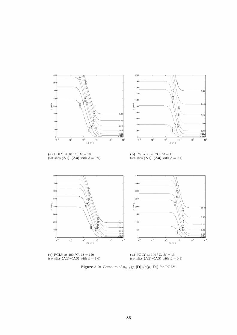
(a) PGLY at 40 C, M = 100(satisfies (A1)–(A3) with β = 0.9)

(b) PGLY at 40 C, M = 11(satisfies (A1)–(A3) with β = 0.1)

(c) PGLY at 100 C, M = 150(satisfies (A1)–(A3) with β = 1.0)

(d) PGLY at 100 C, M = 15(satisfies (A1)–(A3) with β = 0.1)

Figure 5.9: Contours of ηM,B(p, |D|)/η(p, |D|) for PGLY.

85

0.0010.01

0.1

0.1

1

1

1

1

|D| (s−1)

p (M

Pa)

104

106

108

1010

1012

1014

0

200

400

600

800

1000

1200

1400

1600

1800

2000

(a) Contours of IA4 for SQL, T = 40 C.

1e−05

0.00010.001

0.01

0.010.1

0.1

1

1

1

1

|D| (s−1)

p (M

Pa)

104

106

108

1010

1012

1014

0

200

400

600

800

1000

1200

1400

1600

1800

2000

(b) Contours of IA4 for SQL, T = 100 C.

0.01

0.1

0.1

1

1

1

1

|D| (s−1)

p (M

Pa)

104

106

108

1010

1012

1014

0

200

400

600

800

1000

1200

1400

1600

1800

2000

(c) Contours of IA4 for PGLY, T = 40 C.

0.01

0.01

0.1

0.1

1

1

1

1

|D| (s−1)

p (M

Pa)

104

106

108

1010

1012

1014

0

200

400

600

800

1000

1200

1400

1600

1800

2000

(d) Contours of IA4 for PGLY, T = 100 C.

0.0010.01

0.1

0.1

11

1

1

|D| (s−1)

p (M

Pa)

104

106

108

1010

1012

1014

0

200

400

600

800

1000

1200

1400

1600

1800

2000

(e) Contours of IA4 for SQL+PIP, T = 40 C.

0.00010.001

0.01

0.01

0.1

0.1

1

1

11

|D| (s−1)

p (M

Pa)

104

106

108

1010

1012

1014

0

200

400

600

800

1000

1200

1400

1600

1800

2000

(f) Contours of IA4 for SQL+PIP, T = 100 C.

Figure 5.10: Contours of IA4(p,D) (those less than 1) for three reference liquids.

86

Chapter 6

Conclusion

The main results of the thesis have been presented in Chapter 2. We have studied the isother-mal steady flow of a class of incompressible homogeneous fluids whose viscosity depends onpressure and shear rate. The results are based on the approach developed by Malek et al.(2002). In particular, the recent result by Franta et al. (2005) concerned with the steady flowsubject to homogeneous Dirichlet boundary conditions has been generalized in the thesis.

The major improvement consists of including boundary conditions that appear in practicalapplications. In the flows subject to Dirichlet conditions on the entire boundary the level ofpressure in the solution is not naturally determined, and it has to be fixed by an additionalrequirement (e.g., by prescribing the mean value of the pressure over the domain). Note that, incontrast to fluids whose viscosity does not depend on pressure, the level of pressure affects theentire solution of the problem if piezoviscous fluid is involved. Thus, we have been particularlyinterested in boundary conditions involving free inflow/outflow through the boundary and wehave shown that they provide a natural way to determine the level of pressure in the solutionuniquely.

A minor difference in the approach utilized in the provided proofs, compared to previousresults, is related to how we accentuate the discrete approximations. In the previous studiesthe sequence of Galerkin approximations converged to a quasi-compressible approximationof the problem, and then the convergence of these quasi-compressible approximations to the“incompressible” solution of the problem has been shown on a continuous level. Motivatedby the standard finite element method discretization, we have altered this procedure, showingthat the discrete Galerkin approximations (satisfying the discrete incompressibility constraint)converge directly to the weak solution of the problem. Due to this slight modification, therole played by the (discrete) inf–sup conditions in the process has been revealed.

In the second part, we have addressed the numerical approximations. Using a finite elementmethod implemented previously by J. Hron, and used successfully with a number of problemsrelated to incompressible non-Newtonian fluids, we performed a set of experiments. One of ouraims was to examine the behaviour of the numerical method when the assumptions requiredby the current theoretical results are not satisfied. In Chapter 3, we have observed that thenumerical method fails once the changes of the viscosity due to the pressure are too rapid;moreover, we have experimentally identified the condition that seems to determine the failure.Note that the condition is somewhat weaker than the assumptions required to show the well-posedness; in fact, we did not observe any change of behaviour that could be linked to thoseassumptions.

The fluid models considered in the thesis are of great importance in engineering problemsrelated to lubrication. Though our theoretical results may be applicable to other areas (suchas in geology) our main concern has been hydrodynamic lubrication problems, in particularwith the flow in journal bearings. In Chapter 4 we have illustrated the effects due to thepressure-thickening and shear-thinning on the flow in between parallel plates and on the flowin the journal bearing. We have shown a considerable sensitivity of the flow characteristics onthe boundary conditions determining the pressure.

87

We have examined the relevance of the assumptions required by the theoretical results to thethree reference lubricants recently characterized by Bair (2006). We have concluded that theseaccurate models satisfy our assumptions in certain ranges of pressures and shear rates, whileoutside these ranges the assumptions are inevitably violated. The ranges of parameters arequantified in Chapter 5.

88

Bibliography

Amrouche, C. and Girault, V. (1994). Decomposition of vector-spaces and application ot theStokes problem in arbitrary dimension. Czechoslovak Math. J., 44(1):109–140.

Bair, S. (2006). Reference liquids for quantitative elastohydrodynamics: selection and rheo-logical characterization. Tribol. Lett., 22(2):197–206.

Bair, S. and Gordon, P. (2006). Rheological challenges and opportunities for EHL. In Snidle,R. W. and Evans, H. P., editors, IUTAM Symposium on Elastohydrodynamics and Micro-Elastohydrodynamics, volume 134 of Solid Mechanics And Its Applications, pages 23–43.Springer.

Bair, S., Khonsari, M., and Winer, W. O. (1998). High-pressure rheology of lubricants andlimitations of the Reynolds equation. Tribol. Int., 31(10):573–586.

Bair, S. and Kottke, P. (2003). Pressure–viscosity relationship for elastohydrodynamics. Tribol.Trans., 46:289–295.

Bair, S., McCabe, C., and Cummings, P. T. (2002). Comparison of nonequilibrium moleculardynamics with experimental measurements in the nonlinear shear-thinning regime. Phys.Rev. Lett., 88(5):058302.

Ballal, B. Y. and Rivlin, R. S. (1976). Flow of a Newtonian fluid between eccentric rotatingcylinders: inertial effects. Arch. Ration. Mech. Anal., 62(3):237–294.

Barus, C. (1893). Isothermals, isopiestics and isometrics relative to viscosity. Amer. J. Sci.,45:87–96.

Beavers, G. S. and Joseph, D. D. (1967). Boundary conditions at a naturally permeable wall.J. Fluid Mech., 30:197–207.

Bird, R. B., Armstrong, R. C., and Hassager, O. (1987). Dynamics of Polymeric Liquids.John Wiley & Sons.

Bogovskii, M. E. (1980). Solutions of some vector analysis problems connected with operatorsdiv and grad (in Russian). Trudy Sem. S. L. Soboleva, 80(1):5–40.

Bramley, R. and Wang, X. (1995). SPLIB: A library of iterative methods for sparse linearsystem. Technical Report IN 47405, Indiana University–Bloomington.

Bridgman, P. W. (1931). The Physics of High Pressure. MacMillan, New York.

Brindley, J., Elliot, L., and McKay, J. T. (1983). The role of cavitation in whirl instability ina rotor bearing. ASME J. Appl. Mech., 50:877–890.

Bulıcek, M. and Fiserova, V. (2009). Existence theory for steady flows of fluids with pressureand shear rate dependent viscosity, for low values of the power-law index. Z. Anal. Anwend.,28(3):349–371.

Bulıcek, M., Malek, J., and Rajagopal, K. R. (2007). Navier’s slip and evolutionary Navier–Stokes-like systems with pressure and shear-rate dependent viscosity. Indiana Univ. Math.J., 56(1):51–85.

89

Bulıcek, M., Malek, J., and Rajagopal, K. R. (2009a). Analysis of the flows of incompressiblefluids with pressure dependent viscosity fulfilling ν(p, · )→ +∞ as p→ +∞. CzechoslovakMath. J., 59(2):503–528.

Bulıcek, M., Malek, J., and Rajagopal, K. R. (2009b). Mathematical analysis of unsteadyflows of fluids with pressure, shear-rate and temperature dependent material moduli thatslip at solid boundaries. SIAM J. Math. Anal., 41(2):665–707.

Carreau, P. J. (1968). PhD thesis, University of Wisconsin, Madison.

Carreau, P. J. (1972). Rheological equations from molecular network theories. T. Soc. Rheol.,16:99–127.

Davies, T. A. (2004). UMFPACK version 4.3 user guide. Technical Report REP-2004-349,University of Florida, (http://www.cise.ufl.edu/research/sparse/umfpack).

Doolittle, A. K. (1951). Studies in Newtonian flow 2. The dependence of the viscosity of liquidson free-space. J. Appl. Phys., 22(12):1471–1475.

Dowson, D. and Higginson, G. R. (1966). Elastohydrodynamic Lubrication, The Fundamentalsof Roller and Gear Lubrication. Pergamon, Oxford.

Duffing, G. (1924). Attempt at the friction of solid boundaries (in German). Z. Angew. Math.Me., 4:296–314.

Dymond, J. H. and Malhotra, R. (1988). The Tait equation—100 years on. Int. J. Thermo-phys., 9(6):941–951.

Feireisl, E. (2004). Dynamics of viscous compressible fluids, volume 26 of Oxford Lecture Seriesin Mathematics and Its Applications. Oxford Univ. Press.

Feireisl, E. (2007). Mathematical theory of compressible, viscous, and heat conducting fluids.Comput. Math. Appl., 53:461–490.

Ferry, J. D. (1980). Viscoelastic properties of polymers. Wiley, New York, 3rd edition.

Franta, M., Malek, J., and Rajagopal, K. R. (2005). On steady flows of fluids with pressure-and shear-dependent viscosities. Proc. R. Soc. A, 461(2055):651–670.

Gazzola, F. (1997). A note on the evolution of Navier-Stokes equations with a pressure-dependent viscosity. Z. Angew. Math. Phys., 48:760–773.

Gazzola, F. and Secchi, P. (1998). Some results about stationary Navier-Stokes equationswith a pressure-dependent viscosity. In Salvi, R., editor, Navier-Stokes equations: theoryand numerical methods (Varenna, 1997), volume 388 of Pitman Res. Notes Math. Ser.,pages 31–37. Longman, Harlow.

Granick, S., Zhu, Y. X., and Lee, H. (2003). Slippery questions about complex fluids flowingpast solids. Nat. Mater., 2(4):221–227.

Gresho, P. and Sani, R. (2000). Incompressible flow and the finite element method., volume 2:Isothermal laminar flow. John Wiley & Sons Ltd.

90

Gwynllyw, D. R., Davies, A. R., and Phillips, T. N. (1996a). A moving spectral ele-ment approach to the dynamically loaded journal bearing problem. J. Comput. Phys.,123(2):476–494.

Gwynllyw, D. R., Davies, A. R., and Phillips, T. N. (1996b). On the effects of a piezoviscouslubricant on the dynamics of a journal bearing. Journal of Rheology, 40(6):1239–1266.

Gwynllyw, D. R. and Phillips, T. N. (1996). Preconditioned iterative methods for un-steady non-Newtonian flow between eccentrically rotating cylinders. SIAM J. Sci. Comput.,17(6):1369–1394.

Gwynllyw, D. R. and Phillips, T. N. (2005). Some issues regarding spectral element meshesfor moving journal bearing systems. Int. J. Numer. Meth. Fluids, 48:423–454.

Haslinger, J. and Stebel, J. (2011). Shape optimization for Navier–Stokes equations withalgebraic turbulence model: Numerical analysis and computation. Appl. Math. Comput.,63(2):277–308.

Heywood, J. G., Rannacher, R., and Turek, S. (1996). Artificial boundaries and flux andpressure conditions for the incompressible Navier–Stokes equations. Int. J. Numer. Meth.Fluids, 22(5):325–352.

Hirn, A., Lanzendorfer, M., and Stebel, J. (2010). Finite element approximations of flow offluids with shear rate and pressure dependent viscosity. IMA Journal of Numerical Analysis,submitted for publication.

Hron, J. (2001). Fluid structure interaction with applications in biomechanics. PhD thesis,Charles University, Prague, Faculty of Mathematics and Physics.

Hron, J., Malek, J., Necas, J., and Rajagopal, K. R. (2003). Numerical simulations and globalexistence of solutions of two-dimensional flows of fluids with pressure- and shear-dependentviscosities. Math. Comput. Simulation, 61(3-6):297–315. MODELLING 2001 (Pilsen).

Hron, J., Malek, J., Prusa, V., and Rajagopal, K. R. (2011). Further remarks on simple flows offluids with pressure-dependent viscosities. Nonlinear Anal. Real World Appl., 12(1):394–402.

Hron, J., Malek, J., and Rajagopal, K. R. (2001). Simple flows of fluids withpressure-dependent viscosities. Proc. R. Soc. Lond. Ser. A Math. Phys. Eng. Sci.,457(2011):1603–1622.

Hutton, J. F., Jones, B., and Bates, T. W. (1983). Effects of isotropic pressure on the hightemperature high shear viscosity of motor oils. S. A. E., Paper No. 830030:1–11.

Jones, I. P. (1973). Low Reynolds number flow past a porous spherical shell. Proc. Camb.Philos. Soc., 73:231–238.

Kamal, M. M. (1966). Separation in flow between eccentric rotating cylinders. J. Basic Eng.–TASME, 88:717–724.

Kelley, C. T. (2003). Solving nonlinear equations with Newton’s method. SIAM.

Lanzendorfer, M. (2009). On steady inner flows of an incompressible fluid with the viscositydepending on the pressure and the shear rate. Nonlinear Anal.–Real, 10(4):1943–1954.

91

Lanzendorfer, M. and Stebel, J. (2011a). On a mathematical model of journal bearing lubri-cation. Math. Comput. Simulat. In print.

Lanzendorfer, M. and Stebel, J. (2011b). On pressure boundary conditions for steady flows ofincompressible fluids with pressure and shear rate dependent viscosities. Appl. Math.–Czech,56(3):265–285.

Li, X. K., Davies, A. R., and Phillips, T. N. (2000a). A transient thermal analysis for dynam-ically loaded bearings. Comput. Fluids, 29(7):749–790.

Li, X. K., Gwynllyw, D. R., Davies, A. R., and Phillips, T. N. (1999). Three-dimensionaleffects in dynamically loaded journal bearings. Int. J. Numer. Meth. Fluids, 29(3):311–341.

Li, X. K., Gwynllyw, D. R., Davies, A. R., and Phillips, T. N. (2000b). On the influence oflubricant properties on the dynamics of two-dimensional journal bearings. J. Non-NewtonianFluid Mech., 93:29–59.

Malek, J., Necas, J., and Rajagopal, K. R. (2002). Global analysis of the flows of fluids withpressure-dependent viscosities. Arch. Ration. Mech. Anal., 165(3):243–269.

Malek, J., Necas, J., Rokyta, M., and Ruzicka, M. (1996). Weak and measure-valued solutionsto evolutionary PDEs. Chapman & Hall, London.

Malek, J. and Rajagopal, K. R. (2006). Handbook of Differential Equations: Evolutionaryequations, volume 2, chapter 5. Mathematical issues concerning the Navier–Stokes equationsand some of its generalizations, pages 371–459. Elsevier/North-Holland, Amsterdam.

Malek, J. and Rajagopal, K. R. (2007). Handbook of Mathematical Fluid Dynamics, volume 4,chapter 7. Mathematical properties of the solutions to the equations governing the flow offluids with pressure and shear rate dependent viscosities, pages 407–444. Elsevier/North-Holland, Amsterdam.

Malek, J. and Rajagopal, K. R. (2010). Compressible generalized Newtonian fluids. Z. Angew.Math. Phys., 61:1097–1110.

Murnaghan, F. D. (1944). The compressibility of media under extreme pressures. Proc. Natl.Acad. Sci. U. S. A., 30(9):244–247.

Neto, C., Evans, D. R., Bonaccurso, E., Butt, H. J., and Craig, V. S. J. (2005). Boundary slipin Newtonian liquids: a review of experimental studies. Rep. Prog. Phys., 68(12):2859–2897.

Nield, D. A. (2009). The Beavers–Joseph boundary condition and related matters: A historicaland critical note. Transp. Porous Med., 78(3):537–540.

Novotny, A. and Straskraba, I. (2004). Introduction to the Mathematical Theory of Compress-ible Flow, volume 27 of Oxford Lecture Series in Mathematics and its Applications. OxfordUniv. Press, New York.

Oseen, C. W. (1927). Hydrodynamik. Akademische Verlagsgesellschaft M.B.H., Lepzig.

Rajagopal, K. R. (2006). On implicit constitutive theories for fluids. J. Fluid Mech., 550:243–249.

Rajagopal, K. R. and Szeri, A. Z. (2003). On an inconsistency in the derivation of the equationsof elastohydrodynamic lubrication. Proc. R. Soc. A, 459(2039):2771–2786.

92

Reissner, H. (1935). Planar and spatial currents of incompressible, inertia-free liquids betweenexcentric, relative rotating cylinder layers (in German). Z. Anal. Anwend., 15:81–87.

Renardy, M. (1986). Some remarks on the Navier–Stokes equations with a pressure-dependentviscosity. Comm. Part. Diff. Eq., 11:779–793.

Repin, S. I. (2008). A posteriori estimates for partial differential equations, volume 4 of RadonSeries on Computational and Applied Mathematics. Walter de Gruyter, New York.

Reynolds, O. (1886). On the theory of lubrication and its application to Mr. BeauchampTower’s experiments, including an experimental determination of the viscosity of olive oil.Phil. Trans. R. Soc. Lond., 177:157–234.

Saffman, P. (1971). On the boundary condition at the surface of a porous medium. Studiesappl. Math., 50:93–101.

Sani, R. L., Gresho, P. M., Lee, R. L., and Griffiths, D. F. (1981). The cause and cure of thespurious pressures generated by certain FEM solutions of the incompressible Navier–Stokesequations. Int. J. Numer. Methods Fluids, 1:17–43 (Part I), 171–204 (Part II).

Szeri, A. Z. (1998). Fluid Film Lubrication: Theory and Design. Cambridge University Press.

Yasuda, K. (1979). Investigation of the analogies between viscometric and linear viscoelasticproperties of polystyrene fluids. PhD thesis, Massachusetts Institute of Technology, Cam-bridge.

93