flow over aircraft

COM PUTATI ONAL AERODYNAM IC ANALYS IS OF THE FLOW FIELD ABOUT A

HYPERVELOCITY TEST SLED

THESIS

Andrew J. Lofthouse, Captain, USAF

AFIT/GAE/ENY/02-07

DEPARTMENT OF THE AIR FORCE AIR UNIVERSITY

AIR FORCE INSTITUTE OF TECHNOLOGY

Wrigh t-Patter son Air Force Base, Ohio

APPROVED FOR PUBLIC RELEASE; DISTRIBUTION UNLIMITED.

The views expressed in this thesis are those of the author and do not reflect the official

policy or position of the United States Air Force, the Department of Defense or the United

States Government.

AFIT/GAE/ENY/02-07

COMPUTATIONAL AERODYNAMIC ANALYSIS OF THE FLOW FIELD

ABOUT A HYPERVELOCITY TEST SLED

THESIS

Presented to the Faculty

Department of Aeronautics and Astronautics

Graduate School of Engineering and Management

Air Force Institute of Technology

Air University

Air Education and Training Command

In Partial Fulfillment of the

Requirements for the Degree of

Master of Science in Aeronautical Engineering

Andrew J. Lofthouse, BS

Captain, USAF

March 2002

APPROVED FOR PUBLIC RELEASE; DISTRIBUTION UNLIMITED

Acknowledgements

I am eternally grateful for the support and love my wife has shown me. Since the day we

met as undergraduate students, she has inspired and motivated me beyond mere academic

mediocrity. During the past year and a half, this support has continued as she has been

a virtual ”single mom” (as well as full-time graduate student herself) – taking care of our

two children while ”Dad is at school.” The satisfaction of completing this research project

would have been meaningless without having my family by my side throughout the entire

process. I dedicate this work to them.

I am also indebted to Lt Col Monty Hughson for his guidance and insights into the

“finer” aspects of CFD, and for his trust in me that I could accomplish such a work. The

assistance of Lt Col Ray Maple was invaluable as well; not only is he a CFD genius, but

also a rather skilled Linux guru.

Finally, this research wouldn’t have been possible without the financial and technical

support of Dr. Len Sakell of the Air Force Office of Scientific Research, Dr. Michael Hooser

(and others) from the High Speed Test Track Facility at Holloman Air Force Base, New

Mexico, and Dr. Anthony Palazotto.

Andrew J. Lofthouse

iv

Table of Contents

Page

Acknowledgements . . . . . . . . . . . . . . . . . . . . . . . . . . . . . . . . . . iv

List of Figures . . . . . . . . . . . . . . . . . . . . . . . . . . . . . . . . . . . . viii

List of Tables . . . . . . . . . . . . . . . . . . . . . . . . . . . . . . . . . . . . . xiii

List of Symbols . . . . . . . . . . . . . . . . . . . . . . . . . . . . . . . . . . . . xiv

List of Abbreviations . . . . . . . . . . . . . . . . . . . . . . . . . . . . . . . . . xv

Abstract . . . . . . . . . . . . . . . . . . . . . . . . . . . . . . . . . . . . . . . . xvi

I. Introduction . . . . . . . . . . . . . . . . . . . . . . . . . . . . . . . . 1-1

Background . . . . . . . . . . . . . . . . . . . . . . . . . . . . . . 1-1

Previous Work . . . . . . . . . . . . . . . . . . . . . . . . . . . . . 1-3

The “Virtual Wind-Tunnel” . . . . . . . . . . . . . . . . . . . . . 1-4

Research Objectives and Scope . . . . . . . . . . . . . . . . . . . . 1-6

II. Computational Fluid Dynamics General Theory . . . . . . . . . . . . 2-1

Equations of Fluid Flow . . . . . . . . . . . . . . . . . . . . . . . 2-1

Finite Volume Method . . . . . . . . . . . . . . . . . . . . . . . . 2-2

Discretization of the Domain of Interest–Mesh Generation . . . . 2-3

Structured . . . . . . . . . . . . . . . . . . . . . . . . . . . 2-3

Unstructured . . . . . . . . . . . . . . . . . . . . . . . . . . 2-3

Solution Accuracy . . . . . . . . . . . . . . . . . . . . . . . . . . . 2-4

Validation and Verification . . . . . . . . . . . . . . . . . . 2-4

Mesh Independent Solutions . . . . . . . . . . . . . . . . . 2-5

First- and Second-Order Accuracy . . . . . . . . . . . . . . 2-6

Time Accurate Solutions . . . . . . . . . . . . . . . . . . . . . . . 2-7

v

Page

III. Computational Facilities . . . . . . . . . . . . . . . . . . . . . . . . . . 3-1

Hardware . . . . . . . . . . . . . . . . . . . . . . . . . . . . . . . . 3-1

Software . . . . . . . . . . . . . . . . . . . . . . . . . . . . . . . . 3-1

Gridgen . . . . . . . . . . . . . . . . . . . . . . . . . . . . . 3-1

FLUENT . . . . . . . . . . . . . . . . . . . . . . . . . . . . 3-2

Tecplot . . . . . . . . . . . . . . . . . . . . . . . . . . . . . 3-2

IV. Numerical Simulation . . . . . . . . . . . . . . . . . . . . . . . . . . . 4-1

Inviscid, Steady . . . . . . . . . . . . . . . . . . . . . . . . . . . . 4-1

Mesh Generation . . . . . . . . . . . . . . . . . . . . . . . . 4-1

Solver Initialization and Flow Solution . . . . . . . . . . . . 4-17

Mesh Adaptation . . . . . . . . . . . . . . . . . . . . . . . . 4-22

Inviscid, Unsteady . . . . . . . . . . . . . . . . . . . . . . . . . . . 4-24

Solver Initialization and Flow Solution . . . . . . . . . . . . 4-24

V. Results and Discussion . . . . . . . . . . . . . . . . . . . . . . . . . . 5-1

Computational Time . . . . . . . . . . . . . . . . . . . . . . . . . 5-1

Post-Processing Issues . . . . . . . . . . . . . . . . . . . . . . . . 5-3

Definitions . . . . . . . . . . . . . . . . . . . . . . . . . . . . . . . 5-4

Analytical Solutions . . . . . . . . . . . . . . . . . . . . . . . . . . 5-5

Steady, Inviscid Flow . . . . . . . . . . . . . . . . . . . . . . . . . 5-10

Overview of Results . . . . . . . . . . . . . . . . . . . . . . 5-10

Mach 3.0 in Air . . . . . . . . . . . . . . . . . . . . . . . . 5-19

Mach 1.02 in Helium . . . . . . . . . . . . . . . . . . . . . . 5-27

Slipper/Rail Gap . . . . . . . . . . . . . . . . . . . . . . . . . . . 5-33

Unsteady, Inviscid Flow . . . . . . . . . . . . . . . . . . . . . . . . 5-41

VI. Conclusions and Recommendations . . . . . . . . . . . . . . . . . . . . 6-1

Future Work . . . . . . . . . . . . . . . . . . . . . . . . . . . . . . 6-2

vi

Page

Bibliography . . . . . . . . . . . . . . . . . . . . . . . . . . . . . . . . . . . . . BIB-1

Vita . . . . . . . . . . . . . . . . . . . . . . . . . . . . . . . . . . . . . . . . . . VITA-1

vii

List of Figures

Figure

1.1.

1.2.

1.3.

4.1.

4.2.

4.3.

4.4.

4.5.

4.6.

4.7.

4.8.

4.9.

4.10.

4.11.

4.12.

4.13.

4.14.

4.15.

4.16.

4.17.

4.18.

Page

Super Road Runner (SRR) Narrow Gage Sled . . . . . . . . . . . . 1-2

Slipper and Rail Configuration (14:3) . . . . . . . . . . . . . . . . . 1-2

SRR Sled at 4,865 fps in Air (Mach 4.3) . . . . . . . . . . . . . . . 1-2

Experimental Sled Run Trajectory and Corresponding CFD Cases

Modeled . . . . . . . . . . . . . . . . . . . . . . . . . . . . . . . . . 4-2

Technical Drawing of Nike O/U Sled . . . . . . . . . . . . . . . . . 4-2

Modeled Nose Portion of Sled . . . . . . . . . . . . . . . . . . . . . 4-3

Forward Assembly Cut-Away View, Looking Forward . . . . . . . . 4-3

Isometric View of Forward Assembly, Including Slipper/Rail Area . 4-4

Slipper/Rail Assembly Cut-Away Detailed View . .

Modeled Domain Boundaries . . . . . . . . . . . . .

Initial Surface Mesh . . . . . . . . . . . . . . . . . .

Initial Mesh on Rail Surface Near Slipper/Rail Gap

Final Mesh on Rail Surface (M∞ = 3.0 in Air) . . .

Final Mesh on Rail Surface (M∞ = 1.02 in Helium)

. . . . . . . . . 4-4

. . . . . . . . . 4-6

. . . . . . . . . 4-7

. . . . . . . . . 4-8

. . . . . . . . . 4-9

. . . . . . . . . 4-9

Initial Mesh at y = 0 Inches (Bottom Surface of Slipper Wedge) . . 4-10

Initial Mesh at y = −0.0625 Inches (Half-Way Through Gap) . . . . 4-10

Initial Mesh at y = −0.125 Inches (Top Surface of Rail) . . . . . . . 4-11

Adapted Mesh (M∞ = 3.0 in Air) at y = 0 Inches (Bottom Surface of

Slipper Wedge) . . . . . . . . . . . . . . . . . . . . . . . . . . . . . 4-11

Adapted Mesh (M∞ = 3.0 in Air) at y = −0.0625 Inches (Half-Way

Through Gap) . . . . . . . . . . . . . . . . . . . . . . . . . . . . . . 4-12

Adapted Mesh (M∞ = 3.0 in Air) at y = −0.125 (Top Surface of Rail) 4-12

Adapted Mesh (M∞ = 1.02 in Helium) at y = 0 Inches (Bottom

Surface of Slipper Wedge) . . . . . . . . . . . . . . . . . . . . . . . 4-13

viii

Figure Page

4.19. Adapted Mesh (M∞ = 1.02 in Helium) at y = −0.0625 Inches (Half-

Way Through Gap) . . . . . . . . . . . . . . . . . . . . . . . . . . . 4-13

4.20. Adapted Mesh (M∞ = 1.02 in Helium) at y = −0.125 Inches (Top

Surface of Rail) . . . . . . . . . . . . . . . . . . . . . . . . . . . . . 4-14

4.21. Outflow Plane Mesh in Gap Area (Initial Mesh) at x = 23.8 Inches 4-15

4.22. Mesh in Plane at x = 22.6 Inches . . . . . . . . . . . . . . . . . . . 4-15

4.23. Outflow Plane Mesh in Gap Area(M∞ = 3.0) in Air . . . . . . . . . 4-16

4.24. Outflow Plane Mesh in Gap Area (M∞ = 1.02 in Helium) . . . . . . 4-16

4.25. Residual History for M∞ = 3.0 in Air . . . . . . . . . . . . . . . . . 4-20

4.26. Residual History for M∞ = 1.02 in Helium . . . . . . . . . . . . . . 4-20

4.27. Drag Coefficient History for M∞ = 3.0 in Air . . . . . . . . . . . . . 4-21

4.28. Drag Coefficient History for M∞ = 1.02 in Helium . . . . . . . . . . 4-21

5.1. Regions of Flow Defined for Analytic Solution . . . . . . . . . . . . 5-6

5.2. Regions of Flow Defined for Analytic Solution . . . . . . . . . . . . 5-6

5.3. Region 1 Pressure . . . . . . . . . . . . . . . . . . . . . . . . . . . . 5-8

5.4. Detail of Mesh on Payload Cone . . . . . . . . . . . . . . . . . . . . 5-8

5.5. Region 2 Pressure . . . . . . . . . . . . . . . . . . . . . . . . . . . . 5-9

5.6. Region 3 Pressure . . . . . . . . . . . . . . . . . . . . . . . . . . . . 5-9

5.7. Region 4 Pressure . . . . . . . . . . . . . . . . . . . . . . . . . . . . 5-9

5.8. Region 4 Pressure Contours . . . . . . . . . . . . . . . . . . . . . . 5-9

5.9. Region 5 Pressure . . . . . . . . . . . . . . . . . . . . . . . . . . . . 5-10

5.10. Mach Iso-Surface for M∞ = 2.0 in Air (2,200 fps) . . . . . . . . . . 5-11

5.11. Mach Iso-Surface for M∞ = 3.0 in Air (3,300 fps) . . . . . . . . . . 5-12

5.12. Mach Iso-Surface for M∞ = 1.02 in Helium (3,300 fps) . . . . . . . 5-12

5.13. Mach Iso-Surface for M∞ = 2.5 in Helium (8,076 fps) . . . . . . . . 5-13

5.14. Mach Iso-Surface for M∞ = 3.10 in Helium (10,000 fps) . . . . . . . 5-13

5.15. Surface Pressure Contours (psi) for M∞ = 2.0 in Air . . . . . . . . 5-14

ix

Figure Page

5.16. Surface Pressure Contours (psi) for M∞ = 3.0 in Air . . . . . . . . 5-14

5.17. Surface Pressure Contours (psi) for M∞ = 1.02 in Helium . . . . . . 5-15



5.20. Surface Temperature Contours (◦R) for M∞





= 2.0 in Air . . . . . . 5-16

= 3.0 in Air . . . . . . 5-17

= 1.02 in Helium . . . 5-17

= 2.5 in Helium . . . . 5-18

= 3.10 in Helium . . . 5-18

5.25. Surface Density Contours (lbm/ft3) for M∞ = 3.0 in Air . . . . . . 5-19

5.26. Surface Density Contour (lbm/ft3) Detail for M∞ = 3.0 in Air . . . 5-20

5.27. Streamlines at y = 4 Inches in Flow for M∞ = 3.0 in Air . . . . . . 5-20

5.28. Side View of Streamlines in Flow for M∞ = 3.0 in Air. . . . . . . . 5-21

5.29. Front View of Streamlines in Flow for M∞ = 3.0 in Air. . . . . . . . 5-21

5.30. Density Contours (lbm/ft3) at x = 19 Inches for M∞ = 3.0 in Air . 5-22

5.31. Density Contours (lbm/ft3) at y = 3.4 Inches for M∞ = 3.0 in Air . 5-23

5.32. Pressure Contours (psi) at x = 19 Inches for M∞ = 3.0 in Air . . . 5-23

5.33. Pressure Contours (psi) at y = 3.4 Inches for M∞ = 3.0 in Air . . . 5-24

5.34. Temperature Contours (◦R) at x = 19 Inches for M∞ = 3.0 in Air . 5-24

5.35. Temperature Contours (◦R) at y = 3.4 for M∞ = 3.0 in Air . . . . . 5-25

5.36. Velocity Magnitude Contours (ft/s) at x = 19 Inches for M∞ = 3.0 in

Air . . . . . . . . . . . . . . . . . . . . . . . . . . . . . . . . . . . . 5-25

5.37. Velocity Magnitude Contours (ft/s) at y = 3.4 Inches for M∞ = 3.0

in Air . . . . . . . . . . . . . . . . . . . . . . . . . . . . . . . . . . . 5-26

5.38. Surface Density Contours (lbm/ft3) for M∞ = 1.02 in Helium . . . . 5-28

5.39. Density Contours (lbm/ft3) at x = 0 Inches for M∞ = 1.02 in Helium 5-28



x

Figure Page



5.44. Density Contours (lbm/ft3) at y = 5 Inches for M∞ = 1.02 in Helium 5-31

5.45. Pressure Contours (psi) at y = 5 Inches for M∞ = 1.02 in Helium . 5-31

5.46. Temperature Contours (psi) at y = 5 Inches for M∞ = 1.02 in Helium 5-32

5.47. Streamlines in Slipper/Rail Gap Area (y = 0.2 Inches) for M∞ = 3.0

in Air. . . . . . . . . . . . . . . . . . . . . . . . . . . . . . . . . . . 5-34

5.48. Streamlines in Slipper/Rail Gap Area (y = 0.2 Inches) for M∞ = 1.02

in Helium . . . . . . . . . . . . . . . . . . . . . . . . . . . . . . . . . 5-34

5.49. Streamlines in Slipper/Rail Gap Area (y = −0.0625 Inches) for M∞ =

3.0 in Air. . . . . . . . . . . . . . . . . . . . . . . . . . . . . . . . . 5-35

5.50. Streamlines in Slipper/Rail Gap Area (y = −0.0625 Inches) for M∞ =

1.02 in Helium . . . . . . . . . . . . . . . . . . . . . . . . . . . . . . 5-35

5.51. Detail of Slipper/Rail Gap Area (Looking Up Through Transparent

Rail) . . . . . . . . . . . . . . . . . . . . . . . . . . . . . . . . . . . 5-36

5.52. Definitions of Lines Used in Plots (Looking Up Through Rail to Bot-

tom of Slipper Wedge) . . . . . . . . . . . . . . . . . . . . . . . . . 5-37

5.53. Pressure Distribution Along Line 1 (Outlet) . . . . . . . . . . . . . 5-38

5.54. Temperature Distribution Along Line 1 (Outlet) . . . . . . . . . . . 5-38

5.55. Pressure Distribution Along Line 2 (Inboard Side) . . . . . . . . . . 5-39

5.56. Temperature Distribution Along Line 2 (Inboard Side) . . . . . . . 5-39

5.57. Pressure Distribution Along Line 3 (Outboard Side) . . . . . . . . . 5-40

5.58. Temperature Distribution Along Line 3 (Outboard Side) . . . . . . 5-40

5.59. Mass Fraction of Air at t = 1.0 × 10−3 Seconds . . . . . . . . . . . . 5-42

5.60. Mass Fraction of Air at t = 2.0 × 10−3 Seconds . . . . . . . . . . . . 5-42

5.61. Mass Fraction of Air at t = 3.0e − 3 Seconds . . . . . . . . . . . . . 5-43

5.62. Mass Fraction of Air at t = 4.0e − 3 Seconds . . . . . . . . . . . . . 5-43

5.63. Drag Coefficient During Air-to-Helium Transition . . . . . . . . . . 5-44

5.64. Static Pressure (psi) Contours at t = 2.0 × 10−3 Seconds . . . . . . 5-45

xi

Figure

5.65. Static Pressure (psi) Contours at t = 3.0 × 10−3 Seconds





5.70. Static Pressure (psi) Contours at t = 4.5 × 103 Seconds .



Page

. . . . . . 5-46

. . . . . . 5-46

. . . . . . 5-47

. . . . . . 5-47

. . . . . . 5-48

. . . . . . 5-48

. . . . . . 5-49

. . . . . . 5-49

5.73. Surface Static Pressure (psi) Contours at t = 2.0 × 10−3 Seconds . . 5-50









xii

List of Tables

Table Page

4.1. Mach Numbers and Corresponding Velocities Modeled . . . . . . . 4-18

4.2. Mesh Adaptations and Threshold Values Used . . . . . . . . . . . . 4-23

4.3. Final Properties of Adapted Meshes . . . . . . . . . . . . . . . . . . 4-24

5.1. Computation Time . . . . . . . . . . . . . . . . . . . . . . . . . . . 5-2

5.2. Parallel Computation Times . . . . . . . . . . . . . . . . . . . . . . 5-3

5.3. Summary of Analytic Results for M∞ = 3.0 in Air . . . . . . . . . . 5-7

xiii

List of Symbols

Symbol Page

Q, vector of primitive variables . . . . . . . . . . . . . . . . . . . . . . . . . . 2-1

E, flux vector in x-direction . . . . . . . . . . . . . . . . . . . . . . . . . . . 2-1

F, flux vector in y-direction . . . . . . . . . . . . . . . . . . . . . . . . . . . . 2-1

G, flux vector in z-direction . . . . . . . . . . . . . . . . . . . . . . . . . . . 2-1

x, coordinate in x-direction . . . . . . . . . . . . . . . . . . . . . . . . . . . . 2-1

y, coordinate in y-direction . . . . . . . . . . . . . . . . . . . . . . . . . . . . 2-1

z, coordinate in z-direction . . . . . . . . . . . . . . . . . . . . . . . . . . . . 2-1

t, time . . . . . . . . . . . . . . . . . . . . . . . . . . . . . . . . . . . . . . . 2-1

ρ, density . . . . . . . . . . . . . . . . . . . . . . . . . . . . . . . . . . . . . . 2-2

u, velocity component in the x-direction . . . . . . . . . . . . . . . . . . . . . 2-2

v, velocity component in the y-direction . . . . . . . . . . . . . . . . . . . . . 2-2

w, velocity component in the z-direction . . . . . . . . . . . . . . . . . . . . 2-2

et, total energy . . . . . . . . . . . . . . . . . . . . . . . . . . . . . . . . . . . 2-2

p, pressure . . . . . . . . . . . . . . . . . . . . . . . . . . . . . . . . . . . . . 2-2

γ, ratio of specific heats . . . . . . . . . . . . . . . . . . . . . . . . . . . . . . 2-2

e, internal energy . . . . . . . . . . . . . . . . . . . . . . . . . . . . . . . . . 2-2

T , temperature . . . . . . . . . . . . . . . . . . . . . . . . . . . . . . . . . . . 5-4

M , Mach number . . . . . . . . . . . . . . . . . . . . . . . . . . . . . . . . . 5-4

R, specific gas constant . . . . . . . . . . . . . . . . . . . . . . . . . . . . . . 5-4

ft, feet . . . . . . . . . . . . . . . . . . . . . . . . . . . . . . . . . . . . . . . 5-4

lbf , pounds-force . . . . . . . . . . . . . . . . . . . . . . . . . . . . . . . . . . 5-4

lbm, pounds-mass . . . . . . . . . . . . . . . . . . . . . . . . . . . . . . . . . 5-4

Pa, Pascal (N/m2) . . . . . . . . . . . . . . . . . . . . . . . . . . . . . . . . 5-4

xiv

List of Abbreviations

Abbreviation Page

HSTT, High Speed Test Track . . . . . . . . . . . . . . . . . . . . . . . . . . 1-1

SRR, Super Road Runner test sled . . . . . . . . . . . . . . . . . . . . . . . . 1-1

O/U, Over/Under . . . . . . . . . . . . . . . . . . . . . . . . . . . . . . . . . 1-1

fps, feet per second . . . . . . . . . . . . . . . . . . . . . . . . . . . . . . . . 1-3

CFD, computational fluid dynamics . . . . . . . . . . . . . . . . . . . . . . . 1-4

GUI, graphical user interface . . . . . . . . . . . . . . . . . . . . . . . . . . . 1-5

PDE, partial differential equation . . . . . . . . . . . . . . . . . . . . . . . . 2-1

2D, two-dimensional . . . . . . . . . . . . . . . . . . . . . . . . . . . . . . . . 2-4

3D, three-dimensional . . . . . . . . . . . . . . . . . . . . . . . . . . . . . . . 2-4

CDDL, Computational Dynamics and Design Laboratory . . . . . . . . . . . 3-1

AFIT, Air Force Institute of Technology . . . . . . . . . . . . . . . . . . . . 3-1

SGI, Silicon Graphics, Incorporated . . . . . . . . . . . . . . . . . . . . . . . 3-1

MHz, megahertz (103 hertz) . . . . . . . . . . . . . . . . . . . . . . . . . . . 3-1

MB, megabyte (103 bytes) . . . . . . . . . . . . . . . . . . . . . . . . . . . . 3-1

RAM, random access memory . . . . . . . . . . . . . . . . . . . . . . . . . . 3-1

CPU, central processing unit . . . . . . . . . . . . . . . . . . . . . . . . . . . 3-1

GHz, gigahertz (106 hertz) . . . . . . . . . . . . . . . . . . . . . . . . . . . . 3-1

AMD, Advanced Micro Devices . . . . . . . . . . . . . . . . . . . . . . . . . 3-1

GB, gigabyte (106 bytes) . . . . . . . . . . . . . . . . . . . . . . . . . . . . . 3-1

SMP, Symmetric Multi-Processor or Shared Memory . . . . . . . . . . . . . 5-3

xv

AFIT/GAE/ENY/02-07

Abstract

The flow field about the nose section of a hypervelocity test sled is computed using

computational fluid dynamics. The numerical model of the test sled corresponds to the Nike

O/U narrow gage sled used in the upgrade program at the High Speed Test Track facility,

Holloman Air Force Base, New Mexico. The high temperatures and pressures resulting

from the aerodynamic heating and loading affect the sled structure and the performance

of the vehicle. The sled transitions from an air environment to a helium environment at a

speed of approximately 3,300 feet per second (Mach 3 in air, Mach 1.02 in helium) to reduce

the effects of high Mach number flows. Steady, three-dimensional, inviscid flow solutions

are computed for Mach numbers of 2 and 3 in air (2,200 and 3,300 feet per second), and

for Mach numbers of 1.02, 2.5 and 3.1 in helium (3,300, 8,076 and 10,000 feet per second).

Mesh adaptation is used to obtain a mesh-independent solution. Second-order solutions

are obtained for the Mach 3 in air and Mach 1.02 in helium cases. The unsteady transition

from air to helium at 3,300 feet per second is also modeled. Mach 3 in air computations

are compared with analytical results.

xvi

COMPUTATIONAL AERODYNAMIC ANALYSIS

OF THE FLOW FIELD ABOUT A

HYPERVELOCITY TEST SLED

I. Introduction

Background

Hypersonic flight conditions are difficult to replicate without undergoing actual flight

testing. Since flight testing can be expensive and dangerous, other methods are sought

to simulate flight test conditions for hypersonic vehicle systems. One such method is

the ground test facility at the High Speed Test Track (HSTT) at Holloman Air Force

Base, New Mexico. Several types of tests are performed at this facility, including “missile

impact and penetration tests, interceptor tracking tests, material erosion and ablation tests,

aircrew escape system tests, submunition dispenser tests, and tests of inertial guidance

systems” (8:1). The test article is accelerated by a solid rocket booster while riding on

parallel steel crane rails that are approximately 10 miles long.

Figure 1.1 shows one configuration of the hypervelocity sled being developed, called

the Super Road Runner (SRR), during an experimental run. The structure of the SRR

sled is essentially the same as the Nike O/U Narrow Gage sled modeled in this study; the

main difference between the two being the rocket motors used. The sled is attached to

the rails by slippers, which wrap around the rails (Figure 1.2), with a small gap (initially

0.125 inches) between the rail and the slipper. The gap is necessary due to differences in

manufacturing tolerances for the separate sections of track.

As the sled is accelerated to hypersonic speeds, the sled’s supporting structure is

subjected to severe vibrations due to imperfections in the alignment of the parallel rails, as

well as unsteady aerodynamic effects. Occasional severe metal-to-metal contact occurs as

the vibrations “bounce” the sled within the constraints of the slipper-rail gap. This contact

causes rail damage, known as gouging, which was studied recently by Laird (14). Severe

1-1

Figure 1.1 Super Road Runner (SRR) Narrow Gage Sled

Figure 1.2 Slipper and Rail Configuration (14:3)

Figure 1.3 SRR Sled at 4,865 fps in Air (Mach 4.3)

1-2

aerodynamic heating and loading at hypersonic speeds worsen the structural difficulties.

Figure 1.3 illustrates some of the erosive effects encountered during test runs.

During the latter portions of the run, when hypersonic effects would be encountered

in air, the sled is run through a helium environment. Because the speed of sound is higher

in helium than in air, the Mach number is reduced while maintaining a constant ground

speed. This effectively reduces the aerodynamic and aerothermal effects. Due to the reduc-

tion in Mach number, the sled does not experience typical hypersonic phenomena during

acceleration to terminal test velocity. For this reason the sled is termed a hypervelocity

rather than a hypersonic vehicle in this study.

Current sled designs support test velocities of approximately 8,900 feet per second

(fps). The goal for an upgraded design currently in development is to deliver payloads

at velocities approaching 10,000 fps (3:1). A successful upgrade design requires detailed

knowledge of the flow field properties as the sled accelerates to mission speeds, and as

it traverses the air and helium environments. Specifically, knowledge of the pressure field

allows accurate prediction of the aerodynamic drag, which allows proper sizing of the rocket

engines required to attain the final test velocity; and temperature data assist in designing

a slipper-rail system that resists damage due to gouging effects.

Previous Work

Current sled designs are based on empirical methods developed after years of running

different sled configurations at the HSTT. Most new designs do not differ significantly

from previous designs, allowing the use of earlier experimental data. However, for the

design of a significantly different sled, trial runs are necessary to experimentally determine

performance data (19:3-4).

All sled configurations designed and used since the test track was initially developed

in the 1950’s and 1960’s have been analyzed using theoretical methods (such as compress-

ible flow dynamics to determine shock angles, pressures, etc.) and wind-tunnel testing.

Static force tests of early dual rail and monorail sleds were conducted in the von Karman

Gas Dynamics Facility at Arnold Engineering and Development Center (10). However,

1-3

since the design of the current sled is considerably different than those modeled previ-

ously, the earlier wind-tunnel test results are not very useful and are not expected to be

duplicated in this study.

The technical development of monorail variants is reported by Krupovage and Rass-

mussen (13). They discuss solutions to several aerodynamic, structural and thermody-

namic problems to achieve stability control and reduce thermodynamic heating. Korkegi

and Briggs (12, 11) analyzed the flow between the rail and the slipper of a generic sled

using a simplified, two-dimensional approach. They assumed that the flow through the

slipper gap was shock-compressed through a normal (bow) shock off the slipper, and that

the boundary layer rapidly expands to fill the entire gap. Their analysis shows that the

flow is essentially like a supersonic nozzle; the flow accelerates to supersonic speeds at the

entrance to the gap and then, through expansion, the pressure decreases toward the end

of the gap (11:34-36).

As noted before, the current sled design is fairly recent (within the last five years); the

research cited above was finished almost 40 years previously. The Nike sled configuration

has been run experimentally only once, and no aerodynamic data were taken. An early

draft report by Myers (15) gives brief aerodynamic estimates for pressure, temperatures

and Mach numbers for M∞ = 2.0 in air in several regions of interest about the Nike sled

configuration.

The “Virtual Wind-Tunnel”

Hypersonic wind-tunnels are very difficult and expensive to design, build and operate

and, therefore, very few even exist. An alternative to in-flight or wind-tunnel testing of any

hypersonic vehicle is to run computational simulations in so-called “virtual wind-tunnels,”

or computational fluid dynamic (CFD) simulations on high-performance computing plat-

forms.

Several years ago, CFD methods were in their infancy and their use was typically

restricted to research specialists. Combined with computational hardware limitations, this

meant that any computational modeling of a fluid flow was expensive and labor intensive.

1-4

Mesh generation was particularly troublesome and time consuming (and, to an extent,

remains so today). Many of the CFD codes in use required expertise in the numerical

methods used to obtain accurate and stable solutions. Computational models used many

simplifications so that solutions could be obtained in reasonable times.

Today, however, advances in computer hardware and the development of robust

commercial software packages have brought the use of CFD more into the mainstream of

engineering science. Highly sophisticated graphical user interfaces (GUIs) allow relative

ease of use. Robust algorithms for accurate and stable flow modeling don’t require as

much specialization as before. High-end computer workstations and low-cost supercom-

puting clusters provide enough computing power to solve fairly complex flows (including

three-dimensional, viscous flows that take into account chemical reactions) in a reasonable

amount of time.

The ability to simulate hypersonic flows is particularly enticing. CFD simulations

are not subject to experimental inaccuracies, and, because of the deterministic nature

of computers, experimental results are easily duplicated by simply matching the input

conditions. Flow conditions that would be too dangerous or even impossible to replicate in

a wind-tunnel are readily simulated. The number of expensive flight tests can be reduced

by obtaining accurate CFD results to improve a design virtually.

Notwithstanding the positive aspects of CFD simulations, there still remain many

caveats. Despite the advancements with user interfaces and software packages, CFD is

still the work of specialists. Mesh generation is also very much an art, rather than a pure

science. Many solver packages require additional knowledge about the various models so

the user can choose options intelligently.

There are also doubts about the accuracy of CFD simulations. Much work has been

put into defining what is known as validation (solving the right equations) and verification

(solving the equations right). That is, whether or not the computational model does, in

fact, model real, physical flows. The age-old adage of computer programming “garbage in,

garbage out” still applies; CFD results are only as good as the computational models used

to obtain them. Each new code written must be verified by comparing the CFD solutions to

1-5

experimental data and theoretical solutions. Further flight-testing or wind-tunnel testing

is almost always needed to validate each solution before using the CFD code for design or

virtual testing.

Despite these challenges, the “virtual wind-tunnel” remains a cost-effective alterna-

tive to in-flight and wind-tunnel testing. Current research is constantly improving the

state-of-the-art; CFD simulations can only get better.

Research Objectives and Scope

The objective of the current research is to simulate the flow about the nose section of a

hypersonic test sled using commercially available software packages. The temperature and

pressure data obtained are used to support current redesign efforts at the HSTT. The flow

surrounding the nose section is extremely complex, with many shock-shock interactions,

shocks impinging on structural surfaces, reflected shocks from ground effect, possible high-

temperature effects, etc.

The solutions contained herein were obtained for flight conditions similar to test sled

experiments currently being planned. The sled transitions from an air environment to a

helium environment at approximately 3,300 fps (M∞ = 3.0 in air). In this study inviscid,

three-dimensional solutions were obtained for Mach numbers of 2 and 3 in air (velocities of

2,200 and 3,300 fps), and Mach numbers of 1.02, 2.5 and 3.1 in helium (velocities of 3,300,

8,076 and 10,000 fps). The unsteady transition between air and helium was also modeled

at a velocity of 3,300 fps.

Although robust commercial CFD software packages with user-friendly GUIs are

available to reduce the burden of a CFD analysis, there is still considerable effort required

to learn how to use these packages sufficiently well to obtain accurate and stable solutions.

Therefore, a secondary objective of the current research was to evaluate and gain experi-

ence with a suite of commercially available software packages suitable for computational

aerodynamic analysis.

1-6

II. Computational Fluid Dynamics General Theory

The computational analysis of a fluid flow requires an understanding of the general area

of computational fluid dynamics and its application to aerodynamic problems. A typical

CFD analysis goes through a series of distinct steps. Here these steps are given in the

order in which they are performed by the analyst:

• Pre-Processing (Mesh Generation) – the surfaces of the object of interest and the

space around the object (for an external flow) are discretized into a series of grid

points, or nodes. This is similar to the placement of probes in a wind-tunnel experi-

ment.

• Processing (Numerical Computation) – this step includes initializing the flow solver

options to correctly interpret boundary and initial conditions. The solver then com-

putes the flow properties desired at each mesh node.

• Post-Processing (Flow Visualization and Analysis) – once the flow properties have

been computed, the resulting solution is analyzed for relevant trends or relations

using software generally known as scientific visualization tools. Additionally, the

computed solution may be compared to theoretical or experimental results for vali-

dation exercises.

This chapter discusses each of these general steps in the CFD process in more detail,

although not necessarily in the same order.

Equations of Fluid Flow

The physics of a three-dimensional, inviscid flow are described by three sets of partial

differential equations (PDEs). These equations describe the conservation of mass, the

conservation of momentum and the conservation of energy. These equations are known as

the Euler equations and are written here in the flux vector form (6:98)

∂Q

∂t+

∂E

∂x+

∂F

∂y+

∂G

∂z= 0 (2.1)

2-1

where

Q =[

ρ ρu ρv ρw ρet

]T

E =

ρu

ρu2 + p

ρuv

ρuw

(ρet + p) u

, F =

ρv

ρvu

ρv2 + p

ρvw

(ρet + p) v

, G =

ρw

ρwu

ρwv

ρw2 + p

(ρet + p)w

This set of equations is not a closed set; generally, the ideal gas law is chosen to close

the set and make the system mathematically well-posed. The ideal gas law can be written

in the following form

p = ρe(γ − 1) (2.2)

The Euler equations are restricted to flows where the viscous effects are negligible.

Examples are the computations to determine the lift and drag (due to pressure) on an air-

foil. Since boundary layer theory indicates that the pressure gradient normal to the surface

through the boundary layer is negligible, the inviscid flow field outside the boundary layer

can be computed and the resulting pressure distribution approximates the actual pressure

fields with reasonable accuracy. However, inviscid results are not valid for separating flows,

and may predict negative pressures in such cases.

Finite Volume Method

Digital computers cannot solve partial differential equations that describe continuous

physics as shown above. Instead, the equations must be discretized and put into an

algebraic form. Current methods can be categorized into three methods: finite-difference,

finite-volume and finite-element. The finite-volume method will be discussed here.

If the Euler equations are written in integral form for arbitrary control volumes, the

resulting method is known as a finite-volume method. The Euler equations can then be

written as

2-2

∫∫∫

V

(

∂Q

∂t

)

dxdy dz = −∫∫∫

V

(

∂E

∂x+

∂F

∂y+

∂G

∂z

)

dxdy dz (2.3)

where the volume integral is computed over each individual cell.

A finite-volume method does not require a regular, rectilinear (or curvilinear) domain

on which to solve the conservation equations, as would be required with a finite-difference

method. There is a large variety of shapes that can be used for the cell volumes, allowing

great flexibility in generating a mesh. This allows the modeling of complex geometries

with irregularly shaped cells. The effort required to generate a mesh for a finite-volume

solver is usually much less than that required to generate a structured mesh for the same

problem. Additionally, the laws of conservation do not need to be explicitly specified for

the entire domain, since they are specified in the form of the integral equations for each

individual cell volume.

Discretization of the Domain of Interest–Mesh Generation

As mentioned, computers cannot solve the continuous equations and they must be

discretized. The flow field of interest must also be discretized, or covered with a mesh or

grid (the terms can be used interchangeably) of node points. Current CFD technology

uses two types of meshes, structured and unstructured.

Structured. Structured grids are distinguished by having a rectangular compu-

tational (versus physical) domain, with the interior nodes being distributed along distinct

grid lines (7:358). The neighboring nodes of any particular node are implicitly defined by

the indices of those nodes. For example, the neighboring nodes of a node with indices i, j

are i+1, j, i−1, j, i, j−1, etc. Unless the physical domain is also rectangular, the physical

domain must be mapped to the computational domain through a transformation for use in

a finite-difference solver. No such transformation is required with a finite-volume solver.

Structured grids can be used with finite-difference or finite-volume solvers.

Unstructured. Unstructured meshes can be defined as one where the nodes

cannot be associated with regular grid lines (7:359). The elements of an unstructured

2-3

mesh can be any geometric shape. Typically, 2D meshes use triangles or quadrilaterals

and 3D meshes use tetrahedrons and pyramids (6:356). Each node’s neighbors cannot

be determined simply by looking at the indices of the nodes, so additional memory is

consumed (relative to a structured mesh with an equal number of nodes) to hold node-to-

cell mappings. Since the mesh is constructed in the physical domain itself, no coordinate

transformations are needed. Unstructured meshes cannot be used with finite-difference

solvers.

Solution Accuracy

Again, physical flow phenomena are continuous in nature, while the solutions ob-

tained using CFD methods are obtained for discrete points. Therefore, errors are present

in the CFD solutions that must be taken into consideration. Many errors such as trunca-

tion error (from the discretization technique used) and machine round-off error contribute

to the overall error of the solution. Active research is being conducted in areas to improve

the accuracy of solutions (while maintaining numerical stability). This section discusses

some of the important issues related to solution accuracy.

Validation and Verification. The credibility of any computational simulation

must always be addressed. To assist CFD analysts in quantifying “error and uncertainty

in computational simulations,” a process known as Validation and Verification has been

advanced by many CFD researchers and organizations. These two words are not synony-

mous; they both refer to two distinct parts of the process. The definitions given here are

not universally accepted, but they seem to be emerging as the standard. The Guide for

the Verification and Validation of Computational Fluid Dynamics Simulations published

by the American Institute of Aeronautics and Astronautics defines Verification as “the

process of determining if a computational simulation accurately represents the conceptual

model, but no claim is made of the relationship of the simulation to the real world.” Val-

idation is defined as “the process of determining if a computational simulation represents

the real world.” In other words, verification is determining if the computational simulation

2-4

is solving the correct equations (and with the correct order of accuracy), while validation

is ensuring that a physically possible (and correct) solution is obtained (5:1).

Although the present research has been conducted with commercially-available, veri-

fied software, there are pitfalls to blindly accepting the results of such software. As Roache

states in his treatise on validation and verification, “the user must have confidence that

the numerical methods as described in the manuals are actually those implemented in the

code” and that

CFD algorithm developers have long known that there is a trade-off betweencode robustness and accuracy, and CFD code marketers know that there islittle market for numerical accuracy but much demand for bullet-proof coderobustness. General purpose CFD codes must be treated with skepticism inany new application by any conscientious user” (18:10-11).

Due to the lack of experimental data for the Nike sled configuration, the computational

solutions presented in this study can only be compared to relatively simple analytical

solutions.

Mesh Independent Solutions. The accuracy of any CFD simulation is highly

dependent on the mesh used. If there is too little resolution in terms of the number of

nodes to adequately resolve flow features such as shock waves, the solution will be in error.

In addition, too many nodes can negatively impact the computational efficiency. The ideal

mesh would be refined enough to capture all flow features and yet be as coarse as possible

so as to consume less computational resources. A grid-convergence study in which the grid

spacing is systematically reduced until the solution no longer changes can be conducted to

find such a grid. Grid convergence studies are typically conducted with structured meshes

where increasing or decreasing mesh resolution is straightforward.

Mesh Adaptation. Mesh adaptation is a method whereby highly accurate

meshes can be obtained while retaining computation efficiency. The idea behind adapta-

tions is to obtain a highly accurate solution while minimizing the total number of mesh

points used. This is accomplished in two ways; the existing nodes can be redistributed, or

more nodes can be added in order to minimize the errors over the entire flow domain. As

more node points are added, the global error is reduced. Optimizing the number and lo-

2-5

cation of additional nodes requires knowing the locations of the maximum errors, which is

impossible without knowing the exact solution. “Therefore, most adaptive methods rely on

estimating the behavior of the error using feature-detection algorithms. These algorithms

assume regions of high error are associated with regions of high gradients” (22:4). In CFD

applications, this assumption that the highest errors are in the regions of highest gradients

has been proven to be reliable in the resolution of certain flow features, although there is no

guarantee that adapting to high-gradients will improve the accuracy (22:5). Nonetheless,

mesh adaptation remains the best method available to improve the accuracy of solutions

while maintaining computational efficiency, especially for unstructured meshes (in which

case it is arguably as good as, if not better than, a traditional grid convergence study). In

this study, mesh adaptations were performed to obtain mesh-independent solutions.

First- and Second-Order Accuracy. The accuracy of a numerical simulation

is also affected by the order of accuracy of the discretization method used (both temporally

and spatially). The order of the method can be determined by looking at the order of the

dominant truncation error term; a second-order derivative in the error term indicates a

first order solution while a third-order derivative indicates a second-order solutions, etc.

The order of a method determines the effect of dispersion and dissipation errors on the

solutions. For example, a second-order method will usually be dominated by dispersion

error; that is, solution gradients increase, and artificial oscillations can be introduced.

First order methods are usually dominated by dissipation error, where the gradients are

“smeared” out. This dissipation effect can be attributed to second-order error terms that

resemble viscosity terms. For this reason, they are known as “artificial viscosity” terms.

Second-order methods resolve gradients much better than first-order methods; shocks

and other discontinuities tend to be more defined. For this reason, second-order methods

are preferred in CFD. However, the dissipation errors associated with second-order methods

have a tendency to be numerically destabilizing. This can be remedied with the use

of explicit artificial viscosity or limiters. Limiters put limits (obviously) on certain flow

quantities such as temperature or pressure, and so assist in maintaining stability–but this

increase in stability can adversely affect the convergence rate of the solution.

2-6

Time Accurate Solutions

Solutions for steady flows can be obtained by simply dropping the time-dependent

term in Equation (2.1). A steady solution can also be obtained by integrating the govern-

ing equations in time and driving the time derivatives to zero. Although these solutions

use a time step, any intermediate solutions obtained are not necessarily time-accurate be-

cause different time steps can be used for each cell in the flow domain. This procedure

is known as local time-stepping and is frequently used to increase the convergence rate

while maintaining stability. This is possible by decreasing the time step in areas or cells

of decreased stability, while maintaining a larger time-step in solution areas that are more

stable. Time accurate solutions are obtained in a similar manner as steady solutions, with

the exception that a global time step is used. If starting from a physically correct initial

state, the intermediate solutions are also physically correct.

2-7

III. Computational Facilities

The research presented here was accomplished using the computational facilities of the

Computational Dynamics and Design Laboratory (CDDL) of the Department of Aero-

nautics and Astronautics, Graduate School of Engineering and Management, Air Force

Institute of Technology (AFIT). This chapter presents a brief overview of the hardware

and software used during the study.

Hardware

Early mesh generation was accomplished on an SGI Octane2 V6 running IRIX64.

The SGI has dual MIPS R12000A processors running at 360 MHz and has 512 MB of

RAM. Early CFD solutions were obtained on Compaq XP1000 professional workstations

running Tru64 UNIX. Each workstation has an Alpha CPU running at 1 GHz and 512 MB

of RAM. Later solutions were obtained on a 16-node Beowulf class supercomputing cluster,

running Redhat Linux 7.1. Each node consists of two 1.4 GHz AMD Athlon CPUs, 512

MB of RAM and 20 GB of disk space. Some post-processing and some mesh generation

was accomplished on a high-end Dell Precision 530 workstation running Redhat Linux 7.2.

This graphics workstation has dual 1.4 MHz Pentium 4 Xeon processors, 512 MB of RAM

and 37 GB of disk space; it is configured as an access terminal to the Beowulf cluster.

Additional post-processing was accomplished on a Dell Precision 530 workstation running

Microsoft Windows 2000 Professional. The Windows machine has dual 1.7 MHz Pentium

4 Xeon processors and 512 MB of RAM.

Software

All software used for the mesh generation, flow simulation and post-processing is

commercially available. A brief overview of the software packages and their features is

given here.

Gridgen. The meshes used were generated with Gridgen Version 13.3 (on both

the SGI and Linux workstations). Gridgen supports structured, unstructured and hybrid

meshes 17). User input is accomplished through a fairly intuitive GUI.

3-1

FLUENT. Solutions were computed with FLUENT Version 5.5.14 (on the Com-

paq Alpha workstations) and FLUENT Version 6.0.12 (on the Linux cluster). FLUENT is

a general purpose, finite-volume solver; as such, structured and unstructured meshes can

be used. Options are available for several different discretization schemes, including first-

and second-order upwinding. Mesh adaptation using gradients (among other options) is

available to refine or coarsen the mesh (4).

Tecplot. Post-processing was done with Tecplot Version 9.0.2. FLUENT data

can be imported using the FLUENT Data Loader add-on, or by exporting the data from

FLUENT in Tecplot format. However, the FLUENT data exporter does not write the data

in a volume mesh format, so several features of Tecplot (such as iso-surfaces and 3D slices)

are not available. CFD-Analyzer is another add-on available for Tecplot that allows the

computation of several CFD quantities (such as Mach number), the integration of scalars

and vectors along lines, over surfaces and through volumes, the visualization of particle

paths and streaklines as well as error analysis (order of accuracy) (1, 2).

3-2

IV. Numerical Simulation

This chapter discusses the setup of the computational problem, including mesh generation,

flow solver initialization and flow solution.

Inviscid, Steady

Inviscid solutions were obtained for Mach numbers of 2.0 and 3.0 (2,200 and 3,300

fps) in air; and 1.02, 2.1 and 3.10 (3,300, 8,075 and 10,000 fps) in helium. This simulates

an actual test run that transitions from air to helium at about 3,300 fps and continues

to accelerate to the goal of 10,000 fps in the helium environment. After reaching the top

speed required for the test (shown here as 10,000 fps), the actual sled leaves the helium

environment and returns to the air environment. Figure 4.1 illustrates the experimental

run trajectory, as well as the actual flow conditions modeled in this study. As mentioned

previously, the sled transitions from an air environment to a helium environment at about

3,300 fps.

Mesh Generation. Thompson (20) described mesh generation as a “major

pacing item (THE major pacing item were it not for turbulence)” in current CFD methods.

Many industry experts have complained that the majority of the work in obtaining a CFD

solution is expended in the generation of the mesh. This bottleneck in productivity has

been eased somewhat for initial meshes through the use of GUIs. However, GUIs “are

of little or no use to a designer who needs to repeatedly mesh and solve on a series of

similar geometries” (20). One feature that is often overlooked in mesh generation packages

is a non-interactive scripting capability that could be used to batch process many different

configurations of one design.

This trend is also illustrated in the current research; a vast majority of the time

spent was on mesh generation. So much time was spent constructing the initial mesh (and

refining it along the way), that no design iterations were possible for this study.

Model Geometry. The initial model geometry was obtained from technical

drawings (9) of the Nike O/U Hypersonic Upgrade narrow gage rail sled that is currently

4-1

Figure 4.1 Experimental Sled Run Trajectory and Corresponding CFD Cases Modeled

Figure 4.2 Technical Drawing of Nike O/U Sled

under development at the HSTT of Holloman AFB, NM. Figures 4.2-4.6 show portions

of the technical drawings from which the geometry details were extracted. A side view of

the entire sled, consisting of a payload section, several wedges to divert the flow around

structural components (part of forward and rear structural assemblies) and the solid rocket

engine, is shown in Figure 4.2. Figure 4.3 gives a more detailed view of the front portion

that was actually modeled, still from the side. Figure 4.4 is a cut-away view; the cut-away

plane is shown as a broken line in Figure 4.3 (the plane cuts through the slipper wedge).

The front assembly is shown in Figures 4.5-4.6.

The payload modeled is a cylinder-cone combination that sits at the top of the

sled. The cone half-angle is 15◦ and its length is 19 inches (giving a cylinder diameter of

4-2

Figure 4.3 Modeled Nose Portion of Sled

Figure 4.4 Forward Assembly Cut-Away View, Looking Forward

4-3

Figure 4.5 Isometric View of Forward Assem-bly, Including Slipper/Rail Area

Figure 4.6 Slipper/Rail AssemblyCut-Away DetailedView

about 10 inches). A large, vertical wedge extends downward from the payload; this wedge

merges into a rectangular block that sits immediately forward of the rocket motor. A

horizontal strut extends from the sled body on each side and attaches the body to the rail

slippers. Horizontal wedges, called here strut wedges, divert the flow around each strut.

Small vertical wedges, called here slipper wedges, sit immediately ahead of the slippers.

In addition to diverting the flow around the structural components of the sled to improve

aerodynamics, these wedges also shield the structure from the high temperatures and

pressures present in the high-speed flow and assist in braking the sled (when necessary).

The model was truncated at station 23.8259 inches (shown as a broken line in Fig-

ure 4.3) for two primary reasons. First, part of the current research focuses on the flow

field in the gap between the slipper and the rail. Since the flows being studied are super-

sonic, only the flow field features immediately upstream of the forward slipper are needed

to help other researchers assess the gouging damage in the slipper/rail area (14). Second,

inviscid flow solvers cannot handle flow separations. The truncation plane was chosen to

be at station 23.8259 because it sits forward of a void just below the rocket motor and

4-4

above the horizontal strut (Figure 4.3). The flow would surely separate when hitting this

void, causing numerical difficulties.

The rail was modeled as a rectangular block with rounded upper edges. Although

the actual slipper/rail gap is not modeled, the gap between the slipper wedge and the

rail is assumed to be the same height as the slipper/rail gap, which was modeled as 0.125

inches. The initial gap of the sled is about 0.065 inches all around the slipper. During

tests, the slipper material erodes and the gap can range from 0 to 0.125 inches and more.

The height of the rail is 6 inches.

The following coordinate definitions were used: x is positive in the flow direction

with x = 0 being the cone-cylinder intersection; y is positive up, with y = 0 at the lower

surface of the small slipper-wedge; z is positive toward the outboard side of the sled (the

direction in which the strut extends), with z = 0 being at the symmetry plane.

Domain Boundaries. Since flow cannot propagate upstream in supersonic

flows, it is unnecessary to model a large amount of the flow field upstream of the model.

The minimum x distance was set to be at -100 inches (about 80 inches upstream of the cone

point). The maximum y and z distances were chosen based on the expected shock angle.

For all freestream Mach numbers, it is desired that any shocks propagate out through the

outflow domain to keep the boundary conditions constant at freestream conditions for the

forward domain. The maximum shock angle was obtained from Chart 5, NACA Report

1135 (16:48), for the M∞ = 1.02 in helium case. For M∞ = 1.02 around a cone with a

half-angle of 15◦, the shock angle is θ = 75◦. This is simply an estimate since the chart

used is for γ = 1.405 while helium has γ = 5/3. This shock angle gives a minimum ymax

of 160 inches for the shock to exit out of the backplane. The value chosen was ymax = 185

inches to be conservative. Due to the height of the rail (6 inches) and the gap height

(0.125 inches), ymin was -6.125 inches. The outer domain in the z-direction was found by

rotating the y boundary about the z = 0 axis, giving zmax = 191.125 inches. Figure 4.7

shows each of the different boundary zones in the computational model. The individual

faces that comprised the model of the domain of interest were divided into six zones:

pressure-far-field, pressure-outlet, symmetry, ground, rail and body.

4-5

Figure 4.7 Modeled Domain Boundaries

4-6

Figure 4.8 Initial Surface Mesh

Mesh Solver Options. The initial mesh was generated using equal spacing

of the nodes along all edges, with the exception of the rail and the lower surface of the

slipper wedge. The rounded edges of the rail were meshed using a finer, structured mesh to

preserve the curvature. The rectangular cells were converted to triangles by triangulating

along one horizontal.

The node spacings along the sled body edges were ∼ 1 inch (Figure 4.8), and those

along the outer boundaries were ∼ 5 inches. Average node spacing along the rail and

the lower surface of the slipper wedge in the vicinity of the gap was ∼ 0.2 inch. Default

values for the unstructured mesh solver were used to generate the surface meshes and the

interior volume mesh. The initial mesh consisted of 271,038 tetrahedral cells, with 527,668

triangular faces and 52,261 nodes.

Mesh Quality. As mentioned previously, the quality of a mesh can sig-

nificantly influence the quality and stability of the computational solution. In spite of

this fact, very little emphasis was placed on the importance of mesh generation during

this research as it was believed the default options on the mesh solver were sufficient to

4-7

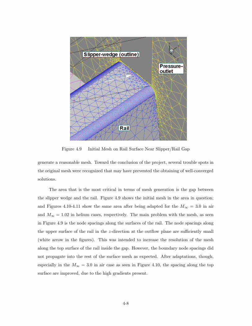
Figure 4.9 Initial Mesh on Rail Surface Near Slipper/Rail Gap

generate a reasonable mesh. Toward the conclusion of the project, several trouble spots in

the original mesh were recognized that may have prevented the obtaining of well-converged

solutions.

The area that is the most critical in terms of mesh generation is the gap between

the slipper wedge and the rail. Figure 4.9 shows the initial mesh in the area in question;

and Figures 4.10-4.11 show the same area after being adapted for the M∞ = 3.0 in air

and M∞ = 1.02 in helium cases, respectively. The main problem with the mesh, as seen

in Figure 4.9 is the node spacings along the surfaces of the rail. The node spacings along

the upper surface of the rail in the z-direction at the outflow plane are sufficiently small

(white arrow in the figures). This was intended to increase the resolution of the mesh

along the top surface of the rail inside the gap. However, the boundary node spacings did

not propagate into the rest of the surface mesh as expected. After adaptations, though,

especially in the M∞ = 3.0 in air case as seen in Figure 4.10, the spacing along the top

surface are improved, due to the high gradients present.

4-8

Figure 4.10 Final Mesh on Rail Surface(M∞ = 3.0 in Air)

Figure 4.11 Final Mesh on Rail Surface(M∞ = 1.02 in Helium)

Figures 4.12-4.14 show the mesh at slices along constant-y planes; specifically, y = 0

inches (the bottom surface of the slipper wedge, or the top of the gap), y = −0.0625 inches

(or half-way through the gap) and y = −0.125 inches (the top surface of the rail or the

bottom of the gap); Figures 4.15-4.17 and Figures 4.18-4.20 show the same areas for the

adapted meshes. The skewness that resulted from inadequate resolution on the top surface

of the rail is seen in Figures 4.12-4.14. The mesh along the bottom surface of the slipper

wedge is finer than that on the top surface of the rail and the result is skewed cells in the

volume as the mesh generator transitions between the two surfaces.

Figures 4.15-4.20 show that the mesh adaptation may have improved the situation.

Due to mesh adaptation, the cells in this region were refined along large pressure gradients

and tended to decrease the skewness. The M∞ = 3.0 in air case shows the most adaptation

in the region, due to large gradients from the impinging shock wave, while the helium case

shows very little adaptation.

Compounding the issue was the lack of adequate resolution in the y-direction, as

shown in Figure 4.21. Figures 4.21 and 4.22 show the initial mesh in two planes; the

pressure-outflow plane at x = 23.8 inches and a slice through the volume at x = 22.6

inches. Figures 4.23-4.24 show the final, adapted meshes in the outflow plane. Comparing

4-9

Figure 4.12 Initial Mesh at y = 0 Inches (Bottom Surface of Slipper Wedge)

Figure 4.13 Initial Mesh at y = −0.0625 Inches (Half-Way Through Gap)

4-10

Figure 4.14 Initial Mesh at y = −0.125 Inches (Top Surface of Rail)

Figure 4.15 Adapted Mesh (M∞ = 3.0 in Air) at y = 0 Inches (Bottom Surface ofSlipper Wedge)

4-11

Figure 4.16 Adapted Mesh (M∞ = 3.0 in Air) at y = −0.0625 Inches (Half-Way ThroughGap)

Figure 4.17 Adapted Mesh (M∞ = 3.0 in Air) at y = −0.125 (Top Surface of Rail)

4-12

Figure 4.18 Adapted Mesh (M∞ = 1.02 in Helium) at y = 0 Inches (Bottom Surface ofSlipper Wedge)

Figure 4.19 Adapted Mesh (M∞ = 1.02 in Helium) at y = −0.0625 Inches (Half-WayThrough Gap)

4-13

Figure 4.20 Adapted Mesh (M∞ = 1.02 in Helium) at y = −0.125 Inches (Top Surfaceof Rail)

the initial mesh to the adapted meshes also shows the same trend mentioned above. Again,

the adapted mesh for the air case shows much more cell refinement due to large gradients.

Adding still more problems is the manner in which the rounded portions of the rail

were meshed. As mentioned previously, these areas were initially meshed with a structured

mesh and converted to an unstructured mesh by diagonalizing each element (to maintain

the curvature resolution of the geometry). The net result is also some very skewed cells.

Comparing the mesh along constant-x planes shows how the resolution along these domains

did not propagate into the volume mesh, as seen in Figures 4.21 and 4.22.

Despite the refinement due to the mesh adaptation, the initial mesh quality may

still have adversely affected the stability and accuracy of the solution. Further studies are

warranted to investigate this possibility.

4-14

Figure 4.21 Outflow Plane Mesh in Gap Area (Initial Mesh) at x = 23.8 Inches

Figure 4.22 Mesh in Plane at x = 22.6 Inches

4-15

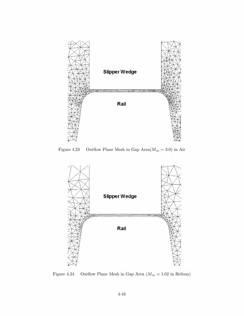
Figure 4.23 Outflow Plane Mesh in Gap Area(M∞ = 3.0) in Air

Figure 4.24 Outflow Plane Mesh in Gap Area (M∞ = 1.02 in Helium)

4-16

Solver Initialization and Flow Solution. The following procedure was used

to set up the solution in FLUENT.

Importing the Mesh. Once the mesh was completed in Gridgen (including

the definition of the boundary zones), it was exported to a FLUENT Version 5 case file.

This case file was read directly into FLUENT. The mesh was checked to ensure that

no negative volumes existed, and a smoothing/swapping procedure was performed (as

recommended) to ensure maximum mesh quality (4:23.11.3). Since the mesh was generated

with units of inches, and FLUENT uses SI units by default, the mesh was scaled, and the

units were changed to use English units everywhere (4:4.2-4.3).

Solver Options. The following options were used to set up the initial so-

lution in FLUENT. Under the define→solver menu, the options for the coupled, explicit,

3D, steady solver with absolute velocity formulation were selected. The viscous model

was set to inviscid and the energy equation was selected. The material was defined to be

an air-helium mixture (to simplify the unsteady modeling of the air-to-helium transition),

with species of air and helium only (no chemical reactions were defined). The density

was modeled as an ideal gas and the specific heat coefficient was modeled using the mix-

ing law (4:13). Operating pressure was set at zero (all pressures computed are absolute

pressures).

The boundary conditions were set as follows. All solid boundaries were modeled as

simple walls (slip boundary conditions with the inviscid solver). These included the body,

the rail and the ground. The symmetry plane used a simple symmetry boundary condition.

The pressure-far-field boundary conditions were set to ambient properties of a standard

day of an altitude of 4,093 feet (corresponding to Holloman AFB, New Mexico). These

conditions were a pressure of 1,821.39 lb/ft2 and a temperature of 504 ◦R. For a supersonic

outflow case, the outlet boundary values are extrapolated from the interior of the domain.

However, in case of reverse flow, the pressure-outlet boundary conditions were set to the

same values as the pressure-far-field values. The Mach number was set according to the

case being run (the initial run used M∞ = 2.0), and the mass fraction was set either to

100% air (as initially run) or 100% helium.

4-17

Table 4.1 Mach Numbers and Corresponding Velocities ModeledM∞ Velocity(fps) Environment

2.0 2,200.3 air

3.0 3,300.4 air

1.0215 3,300 helium

2.5 8,075.6 helium

3.096 10,000.8 helium

Flow Field Initialization. Prior to solving the first case, the flow field

was initialized to freestream conditions, based on the pressure-far-field boundary (this was

M∞ = 2.0 for the first run).

Computation Strategy. The initial flow computed was for M∞ = 2.0

in air. This solution was then used as the initial condition for the M∞ = 3.0 in air

case. The helium solutions were initialized for the M∞ = 1.02 case; that solution was

used as the initial conditions for the M∞ = 2.5 case, which was then used as the initial

condition for the M∞ = 3.10 case. After each solution was iterated for 2,000 iterations (or

until converged), the mesh was adapted and the solution computed again. Second-order

solutions were computed on the final, adapted first-order mesh.

These values of freestream Mach number were chosen based on the velocities of an

actual experimental test run of the hypervelocity sled. The sled initially starts from a

resting position and accelerates to about 3,300 fps in air, at which point it transitions

to the helium environment. This transition point corresponds to the M∞ = 3.0 and

M∞ = 1.02 cases in air and helium, respectively. The sled continues to accelerate in

the helium environment to a (desired) top speed of 10,000 fps, which corresponds to the

M∞ = 3.10 in helium case. The other values for M∞ were chosen arbitrarily for ease of

the solution. Table 4.1 shows the exact Mach numbers and the corresponding velocities

used.

Convergence. As each case was being computed, the residuals were moni-

tored to check for convergence. Residuals are essentially the change in flow field properties

from one iteration to the next. Convergence was defined as being the point at which all

4-18

residuals were reduced by three orders of magnitude. However, due to some inherent flow

instabilities or the low quality of the mesh, only the solution for M∞ = 3.0 in air actually

converged according to this definition, and this only with the initial, unadapted mesh.

Another method of determining the convergence of a solution is to monitor an inte-

grated quantity, such as the drag coefficient. This was done for all cases and the solution

was judged to be converged when the drag coefficient remained relatively constant over

time. To ensure convergence, each of the first-order cases was iterated for 2,000 iterations,

and the second-order cases were iterated for 1,000 iterations.

The residual histories for the air-to-helium transition solutions (3,300 fps) are shown

in Figures 4.25 and 4.26. The reduction of the residuals by three orders of magnitude is

shown in Figure 4.25 (the first 500 iterations) for the M∞ = 3.0 in air case computed

with the unadapted mesh as all the residuals fall below the 10−3 point. Also note that

the spikes in residual values throughout the histories correspond to those points at which

the boundary conditions were changed (for example, from M∞ = 2.0 to M∞ = 3.0) or the

meshes were adapted and the solutions computed again.

Drag Coefficient. As mentioned previously, the drag coefficient was also

monitored. The drag coefficient uses a reference velocity, density and area. The reference

velocity was the freestream velocity corresponding to the Mach number, the reference

density was the ambient density, and the reference area was the frontal area of the sled

body (over which the drag was computed). The values used were

Aref = 1.45 ft2 = 208.15 in2

ρref = 0.00936 lbm/ft3

The drag coefficient histories for the transition cases are shown in Figures 4.27

and 4.28. These plots show that the drag coefficient remains relatively constant with

each of the different, adapted meshes used; it can be argued, then, that these solutions can

be claimed as being independent of the mesh.

4-19

Figure 4.25 Residual History for M∞ = 3.0 in Air

Figure 4.26 Residual History for M∞ = 1.02 in Helium

4-20

Figure 4.27 Drag Coefficient History for M∞ = 3.0 in Air

Figure 4.28 Drag Coefficient History for M∞ = 1.02 in Helium

4-21

Mesh Adaptation. Once the solution was computed for each case, the meshes

were adapted individually to obtain more accurate results. As previously mentioned, since

the objective of mesh adaptation is the reduction in solution error, and since most errors are

in areas of large gradients, the meshes were adapted based on gradients. For compressible

flows, adaptation based on pressure gradients give the best results (4:23.1.2).

Mesh adaptation requires certain guidelines. First, the initial mesh should be fine

enough to resolve the geometry. Second, it should be fine enough to resolve important flow

features such as shock waves. Third, a “reasonably converged” solution should be obtained

prior to the adaptation (4:23.1.2). By using the initial mesh and adapting to the solution

after obtaining a fairly-well converged solution, these guidelines were followed.

The mesh adaptation was performed several times. Each time the adaptation param-

eter was the static pressure gradient. FLUENT adapts the mesh by increasing the number

of nodes and re-triangulating the mesh (when using the conformal node method) for each

cell with a gradient above a certain threshold value. The user specifies the threshold value.

After each adaptation, the mesh was smoothed and cells were swapped to improve the

mesh quality (4:23.11).

The threshold value in each case was determined based on memory constraints as

well as a desire to reduce the maximum pressure gradient per cell in the solution domain as

much as possible. The basic procedure for each case was similar, but the specifics (number

of adaptations and threshold used) varied from case to case. Table 4.2 shows the details of

the adaptations performed. The adaptation number is simply the number of adaptations

performed. The threshold is the pressure gradient threshold (in lbf/ft3) used to determine

which cells needed to be refined. The maximum gradient is the maximum pressure gradient

existing in the solution prior to the adaptation. The cell count is the number of tetrahedral

cells after the adaptation.

In each case, the adaption started with the initial, unadapted mesh of 271,038 cells.

Table 4.3 shows the characteristics of the final, adapted mesh. The final meshes contained

about 2 million cells; more adaptations were not possible due to computer memory con-

straints. Also, the maximum pressure gradients in most cases were less than 1,000 lbf/ft3.

4-22

Table 4.2 Mesh Adaptations and Threshold Values UsedCase Adaptation Threshold Maximum Gradienta Cell Countb

M∞ = 2.0 1 10 2060 461,608air 2 1 1298 1,069,455

3 10 874 1,875,4614 100 845 1,959,300

M∞ = 3.0 1 10 6649 432,003air 2 1 5948 910,403

3 10 3226 1,768,8034 100 1947 1,921,229

M∞ = 1.02 1 10 310 436,469helium 2 1 247 1,377,341

3 10 166 1,563,328

M∞ = 2.5 1 10 4133 455,314helium 2 1 3413 1,022,144

3 10 1889 1,177,6314 50 1281 1,668,122

M∞ = 3.10 1 10 5725 441,439helium 2 1 4030 950,619

3 100 2915 1,152,5044 50 1846 1,772,5245 100 1888 2,153,145

aGradients in lbf/ft3; maximum gradient before adaptation.bCell count after adaptation.

This seems to be the best that can be obtained with current memory restrictions, although

the ideal case would reduce the gradients to O(1). The exceptions to these two statements

are, of course, the M∞ = 3.0 case in air, which has higher maximum gradients; and the

M∞ = 1.02 in helium case, which has a lower number of cells. In each case this is due

to the characteristics of the flow and the magnitude of the pressure gradients (less severe

gradients means less cells required; more severe gradients require more cells).

It should be noted that the adaptations were performed on first-order solutions only.

Following the final adaptations based on the first-order solutions, a second-order solution

was attempted. Stable second-order solutions were obtained only for the M∞ = 3.0 in air

and M∞ = 1.02 in helium cases.

4-23

Table 4.3 Final Properties of Adapted MeshesCase Cell Count Maximum Gradient (lbf/ft3)

M∞ = 2.0 (air) 1,959,300 686

M∞ = 3.0 (air) 1,921,229 1456

M∞ = 1.02 (helium) 1,563,328 117

M∞ = 2.5 (helium) 1,668,122 769

M∞ = 3.1 (helium) 2,153,145 972

Inviscid, Unsteady

All solutions mentioned thus far have been steady computations. These assume that

the properties of the flow are unchanging through time. For the most part, these solutions

should model the actual flow fairly well (assuming a snapshot in time). Additionally, the

changes in flow properties are relatively gradual as the sled accelerates to mission speeds.

However, the transition from the air environment to the helium environment as the

sled enters the helium tent is rather abrupt, and causes some very time-dependent flow

features. Therefore, an unsteady computation was performed to capture the dynamics of

the flow during this transition.

Solver Initialization and Flow Solution. The simplest method to model

the air-to-helium transition is to simply change the boundary conditions on the pressure-

far-field boundary. For this reason the material in the computations was modeled as an

air-helium mixture; it was a simple matter to change the composition of the fluid at the

boundary from 100% air to 100% helium. Additionally, the incoming Mach number was

changed from M∞ = 3.0 (in air) to M∞ = 1.0215 (in helium). In this way, the actual

ground speed remained 3,300 fps.

The mesh used in the unsteady solutions was the initial, unadapted mesh. Adapted

meshes weren’t used for two main reasons. First, the adaptation is solution-specific; the

adaptation used for the M∞ = 3 solution wouldn’t be optimal for a M∞ = 1.02 flow.

Second, since the adaptations are solution specific, the adaptations would have to be

performed at each individual time step. This method was judged to be too prohibitive in

terms of computation time. Therefore, the unsteady computation was initialized using the

M∞ = 3.0 first-order solution on the unadapted mesh.

4-24

FLUENT provides two different ways to perform unsteady computations. One uses

an explicit time integration scheme. With this scheme, the solution after each time-step is

solved in one iteration. The time-step is selected by the solver based on the flow properties.

The user determines how many iterations (thus, how long in time) over which to compute

the solution.

The second method is an implicit method. Here, the user chooses the time-step and

the solution at each time is iterated to convergence. The user also specifies the maximum

number of iterations to perform at each time-step. This is necessary for flows (like the

situation studied here) that may not necessarily meet the convergence criteria (namely, the

reduction in residuals by a specified amount). The user can choose between a first-order

or a second-order implicit time-integration method (4:22.15.1). Since the second-order

solutions showed stability problems, and since the initial data was first-order accurate, the

unsteady computations used the first-order implicit method.

The time-step used was chosen based on the FLUENT recommendation that it

be small enough to allow the solution to converge within about 20 iterations per time-

step (4:22.15.1). The unsteady solution was computed using a time-step of 5 × 10−6

seconds for 1,500 steps (modeling a total of 0.0075 seconds). Previous solutions computed

showed that the unsteadiness in the transition settled out after about 0.0075 seconds. The

maximum number of iterations per time-step was set at 40 in case the solution didn’t con-

verge within the 20 iterations as expected. The convergence criteria remained a reduction

of the residuals by three orders of magnitude.

FLUENT allows the user to animate the flow solution during an unsteady solution.

This is done by taking snapshots of flow property contours or other plots of certain vari-

ables. Animations of pressure contours, species mass fraction, temperature contours, etc.

were thus obtained by taking snapshots every four time-steps (or every 2e-5 seconds). The

data file was also automatically saved every 20 time-steps (to be visualized in Tecplot).

4-25

V. Results and Discussion

As mentioned previously, second-order solutions were obtained only for the V∞ = 3, 300

fps cases (the air-to-helium transition regime); oscillations of flow properties, possibly

attributed to the implicit use of limiters for numerical stability and robustness, restricted

solutions for the other cases to first-order accuracy. The results presented here will focus on

the second-order cases, although they will be compared to the first-order results to illustrate

the effect of Mach number. The first-order, unsteady results will also be presented briefly.

All results given are for static quantities (temperature and pressure) versus stagnation or

total quantities.

Computational Time

In each case for which solutions were computed, the final meshes were close to 2

million cells, as were shown in Table 4.3. This required a significant amount of computa-

tional resources, both in CPU time and memory required. Table 5.1 gives a summary of

the computational time required to run 1,000 iterations in each case. These computations

were performed on the Beowulf class cluster. The wall clock times are not exact; all so-

lutions given here were run in batch mode so the exact time is unknown. FLUENT gives

an estimate of the time remaining for the number of iterations requested throughout the

computation. If the solutions converges prior to completing the requested number of iter-

ations, the time shown is more than the actual time. This is the case in the two situations

where the solution did converge (according to the reduction of residuals by three orders of

magnitude criteria).

The advantage of using parallel processing is illustrated in Table 5.2. The time

required to compute 1000 iterations for the M∞ = 3.0 in air case with the unadapted,

271,038 cell mesh on two different platforms is shown. There is a large difference in the

time taken when using only one processor on each machine, but there is very little difference

when using two processors (two networked workstations were used for the two-processor

Compaq Alpha case, while one dual-processor node was used for the two-processor Linux

cluster case). This is most likely due to the smaller amount of memory on the Compaq

5-1

Table 5.1 Computation TimeCase Adaptation Cell Count # CPUs Wall Clock Time (hours:minutes)

M∞ = 2.0 none 271,038 2 1:30air 1 461,608 2 2:15

2 1,069,455 2 5:453 1,875,461 4 5:204 1,959,300 4 4:30

M∞ = 3.0 none 271,038 2 1:30*air 1 432,003 2 2:00

2 910,403 2 4:10*3 1,768,803 2 8:304 1,921,229 4 4:30

2nd order 1,921,229 4 8:15

M∞ = 1.02 none 271,038 2 1:30helium 1 436,469 2 2:05

2 1,377,341 2 6:453 1,563,328 2 8:00

2nd order 1,563,328 4 7:30

M∞ = 2.5 none 271,038 2 1:40helium 1 455,314 2 3:00

2 1,022,144 2 5:253 1,177,631 2 5:404 1,668,122 2 8:00

M∞ = 3.10 none 271,038 2 1:25helium 1 441,439 2 2:10

2 950,619 2 5:053 1,152,504 2 5:304 1,772,524 2 20:005 2,153,145 4 5:30

unsteady none 271,038 8 24:00

*Met convergence criteria of a residual reduction by three orders of magnitude.

5-2

Table 5.2 Parallel Computation Times# CPU Machine Time (h:m:s) Network Protocol FLUENT Version

1 Compaq Alpha 4:14:17 N/A2 Workstation 1:13:05 Ethernet (sockets) 5.5.14

1 3:11:46 N/A2 1:03:36 SMP4 0:41:27 Ethernet (sockets)8 Linux Cluster 0:27:43 Ethernet (sockets) 6.0.122 1:03:48 Myrinet (sockets)4 0:41:13 Myrinet (sockets)8 0:27:56 Myrinet (sockets)

Alpha workstations; if the entire computational problem doesn’t fit in physical memory,

more time is required due to memory swap operations. There is practically no difference

in the compute times when comparing the use of the Ethernet and Myrinet networks. This

can be explained in two ways; either there is very little communication occurring during

the computations, or the socket interface used in both cases gives similar communication

results. Also note that two different versions of FLUENT were used on the different

architectures, and the computation times may have been influenced by improvements made

in the new version. However, the full benefits of the higher-speed Myrinet network were

not utilized; message passing libraries using the lightweight GM network protocol would

take advantage of its capabilities. In general, though, FLUENT shows excellent parallel

performance.

Post-Processing Issues

One significant drawback in using different commercial software packages for the

different steps in a CFD analysis (i.e., mesh generation, computation, visualization) is the

portability and compatibility of data file formats between the different software packages.

Porting the mesh between Gridgen and FLUENT was not a problem because Gridgen

supports FLUENT Version 5 file formats. However, porting data between FLUENT and

Tecplot became an issue.

FLUENT supports exporting data files to a Tecplot format. However, FLUENT

writes the Tecplot data using a triangular (area) format, rather than a tetrahedral (vol-

5-3

ume) format, even for the volume interior. Some of Tecplot’s 3D features (iso-surface

visualization and 3D slices) require the data to be in a volume format.

Tecplot, on the other hand, also supports importing FLUENT case and data files.

The problem here is that FLUENT stores the data at the cell centers, while Tecplot

requires the data to be at the node points. The FLUENT importer add-on for Tecplot

works around this by interpolating the data at the cell centers to find the values at the

node points. Unfortunately, the data at the boundary zones gets lost in this conversion and

therefore, the data sets imported in this way does not contain data (pressure, temperature,

velocity, etc) on the boundary zones, and no surface contour plots can be generated.

These issues were resolved by using portions of both data sets for different zones.

The data exported by FLUENT into Tecplot format was used for the surface (boundary)

zones, and the data imported by Tecplot from FLUENT was used for the interior volume

data. In this way, all the features of Tecplot were available. Future work using FLUENT

as the flow solver should be done using a scientific visualization software package that

directly supports FLUENT data formats without the loss of surface data.

Definitions

The basic variables that were initially used in the data files were mesh coordinates

(x, y, z), velocities (u, v, w), static temperature (T ), static pressure (p) and density (ρ).

Other variables were computed from these using the CFD Analyzer Tecplot add-on (for

Mach number and pressure coefficient) and directly specifying the equations in Tecplot

(x-, y- and z- momentum and velocity magnitude). The definitions of these variables used

in the computations are (1:63-68)

‖U‖ =√

(u2 + v2 + w2) velocity magnitude (5.1)

M =‖U‖√γRT

Mach number (5.2)

x − momentum = ρu (5.3)

y − momentum = ρv (5.4)

5-4

z − momentum = ρw (5.5)

Cp =p − p∞

ρ∞U2∞

/2(5.6)

where the reference quantities were specified according to a standard day at an

altitude of 4,093 feet (or 1,247.5 meters) for Holloman AFB, NM (21).

p∞ = 87210.4 Pa = 1821.39 lbf/ft2 = 12.65 psi

T∞ = 280 K = 504 R

ρ∞ = 1.08486 kg/m3

Rair = 287 J/(kg K)

γair = 7/5

Rhelium = 2078 J/(kg K)

γhelium = 5/3

Analytical Solutions

Analytic solutions for several regions of the flow surrounding the sled were computed

using simple oblique shock relations for 2D wedges and axisymmetric cones. Figures 5.1

and 5.2 show the regions that were used. The freestream conditions used matched the

conditions for the M∞ = 3.0 in air case (with p∞ = 12.65 psi). The analytic solutions are

summarized in Table 5.3. Figures 5.3-5.7 compare these analytic results to the computed

results. The data for the computed results were obtained by extracting data along polylines

in Tecplot.

Region 1 contains the flow after the shock generated from the payload cone. The

flow was modeled as a simple, supersonic cone. The freestream conditions were used as

the input conditions, and the pressure after the shock (along the surface of the cone) was

obtained using NACA Report 1135 (16). Computational data was taken along the upper

surface of the cone at the symmetry plane. Figure 5.3 shows that the computational results

agree fairly well with the theoretical with the exception of the large oscillations near the

5-5

Figure 5.1 Regions of Flow Defined for Analytic Solution

Figure 5.2 Regions of Flow Defined for Analytic Solution

5-6

Table 5.3 Summary of Analytic Results for M∞ = 3.0 in AirRegion Geometry Input Conditions Pressure (psi)

1 15◦ Cone Freestream 26.55

2 19.65◦ Wedge Freestream 47.01

3 19.65◦ Expansion Region 2 13.15



upstream point. This is most likely due to the faceted nature of the mesh, as shown in

Figure 5.4. Even though the data was extracted along the symmetry plane, where the

mesh is smooth, the data still retain some of the effects of the uneven mesh, most likely

due to interpolations from cell-centered data to node-centered data.

Region 2 is the flow along the lower portion of the large, vertical wedge. Simple

oblique shock relations were used to calculate the pressures downstream of the attached

shock. Freestream conditions were used as input conditions. Computational data was

taken along a line from the vertical wedge leading edge to the shoulder, at y = 4 inches.

The Region 2 data also compare well with the analytical results, as shown in Figure 5.5.

After the initial compression through the shock, the pressure remains fairly constant as

predicted, but then drops off. This is due to three-dimensional effects. While the analytical

results are only valid for a strictly two-dimensional wedge, the actual modeled wedge is

three-dimensional. As the flow expands around the bottom of the wedge, the pressure

decreases.

Region 3 uses Region 2 values as the input values. The flow here expands around

the shoulder of the vertical wedge. Prandtl-Meyer relations were used to compute the flow

properties. Region 3 computational data continued from the Region 2 data back to about

x = 20 inches (just above the strut wedge), at y = 4 inches. The data follows the constant

trend predicted, but the magnitude is lower, as seen in Figure 5.6. The analytical results

used the higher pressures predicted for Region 2 as the input values, but the actual values

were lower due to the expansion around the bottom surface. This caused the pressure

magnitude in Region 3 to be lower than expected.

5-7

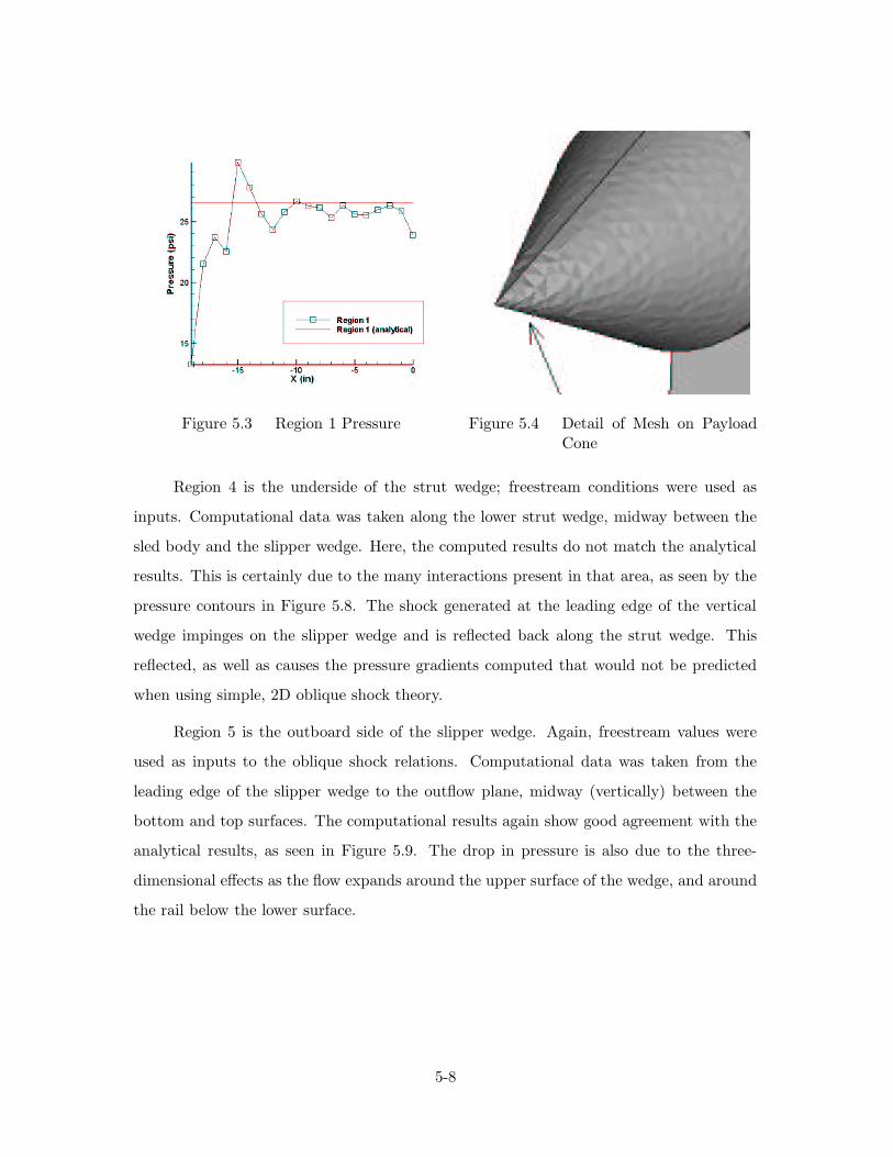
Figure 5.3 Region 1 Pressure Figure 5.4 Detail of Mesh on PayloadCone

Region 4 is the underside of the strut wedge; freestream conditions were used as

inputs. Computational data was taken along the lower strut wedge, midway between the

sled body and the slipper wedge. Here, the computed results do not match the analytical

results. This is certainly due to the many interactions present in that area, as seen by the

pressure contours in Figure 5.8. The shock generated at the leading edge of the vertical

wedge impinges on the slipper wedge and is reflected back along the strut wedge. This

reflected, as well as causes the pressure gradients computed that would not be predicted

when using simple, 2D oblique shock theory.

Region 5 is the outboard side of the slipper wedge. Again, freestream values were

used as inputs to the oblique shock relations. Computational data was taken from the

leading edge of the slipper wedge to the outflow plane, midway (vertically) between the

bottom and top surfaces. The computational results again show good agreement with the

analytical results, as seen in Figure 5.9. The drop in pressure is also due to the three-

dimensional effects as the flow expands around the upper surface of the wedge, and around

the rail below the lower surface.

5-8

Figure 5.5 Region 2 Pressure Figure 5.6 Region 3 Pressure

Figure 5.7 Region 4 Pressure Figure 5.8 Region 4 Pressure Contours

5-9

Figure 5.9 Region 5 Pressure

Steady, Inviscid Flow

Given that the present results do not include any viscous effects, the temperature

distributions presented will not agree with experimental results in magnitude, but the

general trends should be similar. On the other hand, since boundary-layer analysis shows

that the pressure gradient normal to the surface through an attached boundary-layer is

negligible, the pressure distributions presented should be fairly close to those experienced

by the actual sled under the same conditions.

Overview of Results. The computational results for all computed cases (in-

cluding the first-order solutions) are presented here. A more detailed analysis of the two

second-order solutions will follow.

High-speed, inviscid flow properties are affected by discontinuities in the flow field,

such as shock waves and expansion waves. The location of these features depends on

the freestream Mach number and the body geometry. Figures 5.10-5.14 show the general

shape of the shock waves generated by the sled at different Mach numbers and in different

environments. The shocks are visualized in each case by an iso-surface for a Mach number

just below the freestream Mach number.

These figures show that the bow shock impinges on the sled structure at different

points for the different freestream Mach numbers. The location of the shock impingement

5-10

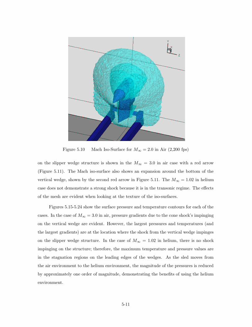
Figure 5.10 Mach Iso-Surface for M∞ = 2.0 in Air (2,200 fps)

on the slipper wedge structure is shown in the M∞ = 3.0 in air case with a red arrow

(Figure 5.11). The Mach iso-surface also shows an expansion around the bottom of the

vertical wedge, shown by the second red arrow in Figure 5.11. The M∞ = 1.02 in helium

case does not demonstrate a strong shock because it is in the transonic regime. The effects

of the mesh are evident when looking at the texture of the iso-surfaces.

Figures 5.15-5.24 show the surface pressure and temperature contours for each of the

cases. In the case of M∞ = 3.0 in air, pressure gradients due to the cone shock’s impinging

on the vertical wedge are evident. However, the largest pressures and temperatures (and

the largest gradients) are at the location where the shock from the vertical wedge impinges

on the slipper wedge structure. In the case of M∞ = 1.02 in helium, there is no shock

impinging on the structure; therefore, the maximum temperature and pressure values are

in the stagnation regions on the leading edges of the wedges. As the sled moves from

the air environment to the helium environment, the magnitude of the pressures is reduced

by approximately one order of magnitude, demonstrating the benefits of using the helium

environment.

5-11

Figure 5.11 Mach Iso-Surface for M∞ = 3.0 in Air (3,300 fps)

Figure 5.12 Mach Iso-Surface for M∞ = 1.02 in Helium (3,300 fps)

5-12



5-13

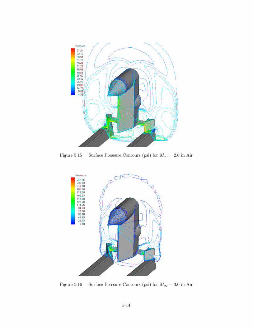
Figure 5.15 Surface Pressure Contours (psi) for M∞ = 2.0 in Air

Figure 5.16 Surface Pressure Contours (psi) for M∞ = 3.0 in Air

5-14

Figure 5.17 Surface Pressure Contours (psi) for M∞ = 1.02 in Helium


5-15


Figure 5.20 Surface Temperature Contours (◦R) for M∞ = 2.0 in Air

5-16

Figure 5.21 Surface Temperature Contours (◦R) for M∞ = 3.0 in Air

Figure 5.22 Surface Temperature Contours (◦R) for M∞ = 1.02 in Helium

5-17



5-18

Figure 5.25 Surface Density Contours (lbm/ft3) for M∞ = 3.0 in Air

Mach 3.0 in Air. Discontinuities in the flow properties are evidence of flow

features that may be of interest (such as shock waves, expansion fans and contact surfaces).

Density contour plots tend to show these discontinuities better than plots of other prop-

erties (such as pressure and temperature). Figure 5.25 shows the density contours for the

M∞ = 3.0 in air case. There is a region of high density where the bow shock impinges on

the slipper wedge structure. This area is discussed in more detail below. Figure 5.26 also

shows the density contours, but with decreased levels of contours, giving more resolution

to the lower density areas. An area of low density around the lower edge of the vertical

wedge can be clearly seen. This suggests that the flow expands around the edge. The

streamlines visualized in Figures 5.27-5.29 show that this is the case. As the flow hits the

vertical wedge, portions of the flow escape underneath the wedge, accelerating around the

corner and creating the lower density areas. Farther back, this expansion causes part of

the flow to go underneath the strut. This flow diversion could cause an upward (lift) force

on the front of the sled. The structural design and performance prediction of the sled

depends on an accurate knowledge of the lift forces present.

5-19

Figure 5.26 Surface Density Contour (lbm/ft3) Detail for M∞ = 3.0 in Air

Figure 5.27 Streamlines at y = 4 Inches in Flow for M∞ = 3.0 in Air

5-20

Figure 5.28 Side View of Streamlines in Flow for M∞ = 3.0 in Air.

Figure 5.29 Front View of Streamlines in Flow for M∞ = 3.0 in Air.

5-21

Figure 5.30 Density Contours (lbm/ft3) at x = 19 Inches for M∞ = 3.0 in Air

Figure 5.30-5.37 show the flow features in the region where the shock impinges on

the sled structure. Slices of the data are taken in the x = 19 and y = 3.4 inch planes.

The shock generated by the vertical wedge hits the slipper wedge and reflects. However,

the shock reflection then interacts with the expansion wave from the vertical wedge and

also impinges on the surface of the strut wedge. These combined effects create a pocket of

stagnated air (see the velocity contours in Figures 5.36 and 5.37) which, in turn, creates the

high temperatures and pressures observed. These strong gradients would cause vibrations

and heating on ablation regions that would adversely impact the sled performance and

contribute to the gouging phenomenon in the slipper/rail gap.

5-22

Figure 5.31 Density Contours (lbm/ft3) at y = 3.4 Inches for M∞ = 3.0 in Air

Figure 5.32 Pressure Contours (psi) at x = 19 Inches for M∞ = 3.0 in Air

5-23

Figure 5.33 Pressure Contours (psi) at y = 3.4 Inches for M∞ = 3.0 in Air

Figure 5.34 Temperature Contours (◦R) at x = 19 Inches for M∞ = 3.0 in Air

5-24

Figure 5.35 Temperature Contours (◦R) at y = 3.4 for M∞ = 3.0 in Air

Figure 5.36 Velocity Magnitude Contours (ft/s) at x = 19 Inches for M∞ = 3.0 in Air

5-25

Figure 5.37 Velocity Magnitude Contours (ft/s) at y = 3.4 Inches for M∞ = 3.0 in Air

5-26

Mach 1.02 in Helium. The same effects that create the large gradients in the

M∞ = 3.0 in air case are not seen in the M∞ = 1.02 in helium case. This demonstrates

the positive aspects of running in a helium environment; while the actual velocity of the

sled is the same in both cases (3,300 fps), the same aerodynamic heating and loading is

not seen in the helium environment because of the lower Mach number.

The density contours shown in Figure 5.38 suggest that the main regions of interest

(those where there is high heating and loading) are simply those on the leading edges of

the various wedges. Since there are no shocks reflecting off the structures, the stagnation

points on the leading edges are the locations of highest temperatures and pressures.

Figures 5.39-5.43 show the density contours on constant-x planes. The flow stagnates

at the leading edge of the large vertical wedge, then is mildly expanded along the wedge.

At the shoulder of the wedge, the flow expands rapidly. The flow above the rounded blister

immediately ahead of the rocket motor stays at the lower density achieved by the expansion

around the shoulder, while the flow below the blister is compressed due to the compression

caused by the stagnated flow near the strut wedge.

The fact that the flow is relatively simple is also shown by the constant-y plane

contours in Figures 5.44-5.46. The flow stagnates at the leading edge, expands mildly

along the leading edge of the vertical wedge, and then rapidly expands at the wedge

shoulders. There are also stagnation regions on the leading edges of the slipper wedges.

The pressures and temperatures are highest when the flow is compressed and are lowest in

the expansion regions.

5-27

Figure 5.38 Surface Density Contours (lbm/ft3) for M∞ = 1.02 in Helium

Figure 5.39 Density Contours (lbm/ft3) at x = 0 Inches for M∞ = 1.02 in Helium

5-28



5-29



5-30

Figure 5.44 Density Contours (lbm/ft3) at y = 5 Inches for M∞ = 1.02 in Helium

Figure 5.45 Pressure Contours (psi) at y = 5 Inches for M∞ = 1.02 in Helium

5-31

Figure 5.46 Temperature Contours (psi) at y = 5 Inches for M∞ = 1.02 in Helium

5-32

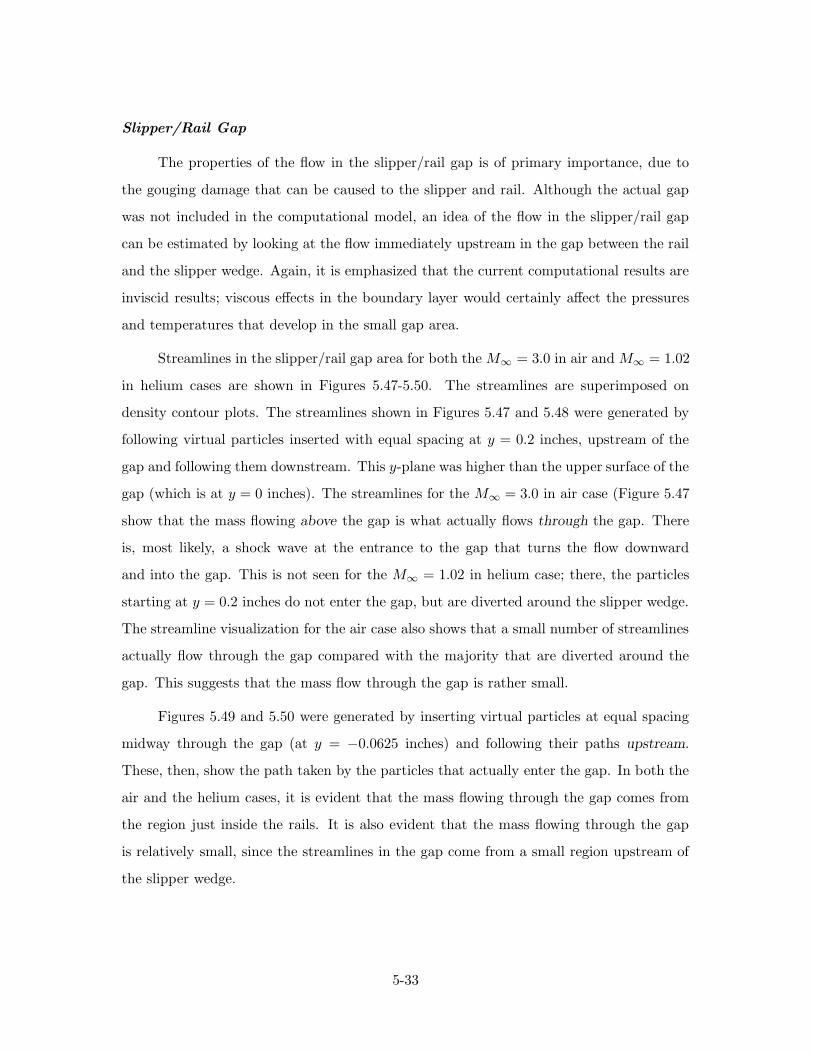
Slipper/Rail Gap

The properties of the flow in the slipper/rail gap is of primary importance, due to

the gouging damage that can be caused to the slipper and rail. Although the actual gap

was not included in the computational model, an idea of the flow in the slipper/rail gap

can be estimated by looking at the flow immediately upstream in the gap between the rail

and the slipper wedge. Again, it is emphasized that the current computational results are

inviscid results; viscous effects in the boundary layer would certainly affect the pressures

and temperatures that develop in the small gap area.

Streamlines in the slipper/rail gap area for both the M∞ = 3.0 in air and M∞ = 1.02

in helium cases are shown in Figures 5.47-5.50. The streamlines are superimposed on

density contour plots. The streamlines shown in Figures 5.47 and 5.48 were generated by

following virtual particles inserted with equal spacing at y = 0.2 inches, upstream of the

gap and following them downstream. This y-plane was higher than the upper surface of the

gap (which is at y = 0 inches). The streamlines for the M∞ = 3.0 in air case (Figure 5.47

show that the mass flowing above the gap is what actually flows through the gap. There

is, most likely, a shock wave at the entrance to the gap that turns the flow downward

and into the gap. This is not seen for the M∞ = 1.02 in helium case; there, the particles

starting at y = 0.2 inches do not enter the gap, but are diverted around the slipper wedge.

The streamline visualization for the air case also shows that a small number of streamlines

actually flow through the gap compared with the majority that are diverted around the

gap. This suggests that the mass flow through the gap is rather small.

Figures 5.49 and 5.50 were generated by inserting virtual particles at equal spacing

midway through the gap (at y = −0.0625 inches) and following their paths upstream.

These, then, show the path taken by the particles that actually enter the gap. In both the

air and the helium cases, it is evident that the mass flowing through the gap comes from

the region just inside the rails. It is also evident that the mass flowing through the gap

is relatively small, since the streamlines in the gap come from a small region upstream of

the slipper wedge.

5-33

Figure 5.47 Streamlines in Slipper/Rail Gap Area (y = 0.2 Inches) for M∞ = 3.0 in Air.

Figure 5.48 Streamlines in Slipper/Rail Gap Area (y = 0.2 Inches) for M∞ = 1.02 inHelium

5-34

Figure 5.49 Streamlines in Slipper/Rail Gap Area (y = −0.0625 Inches) for M∞ = 3.0in Air.

Figure 5.50 Streamlines in Slipper/Rail Gap Area (y = −0.0625 Inches) for M∞ = 1.02in Helium

5-35

Figure 5.51 Detail of Slipper/Rail Gap Area (Looking Up Through Transparent Rail)

Pressure and temperature data was also taken along the lower surface of the slipper

wedge shown in Figure 5.51 along three lines as defined in Figure 5.52. Line 1 runs along

the outflow plane in the z-direction. Line 2 runs along the inboard side of the slipper wedge

in the x-direction. Line 3 runs along the outboard side of the slipper wedge. The lengths in

each case have been normalized to run from 0 to 1. The data were taken along each of the

lines at the surface of the wedge (y = 0 inches), the middle of the gap (y = −0.0625 inches)

and at the upper rail surface (y = −0.125 inches), and are plotted in Figures 5.53-5.58.

The properties in each case are relatively independent of the y-position (vertically), with

the possible exception of Line 2 (inboard edge of the slipper wedge).

The pressure and temperature distributions along the outflow plane (Figures 5.53 and

5.54) follow similar trends. For the air case, the pressures and temperatures are highest on

the inboard side after being compressed through the shock generated by the strut wedge;

they decrease along the outboard side due to the expansion of the air past the edge of the

rail (the flow is forced along the wedge and then expands downward at the edge of the

5-36

Figure 5.52 Definitions of Lines Used in Plots (Looking Up Through Rail to Bottom ofSlipper Wedge)

rail). Since there is no shock generated in the helium case, the pressure and temperatures

are much lower than in the air.

The effects of the shock impinging on the wedge surface are clearly seen in the plots

along the inboard side (Figures 5.55 and 5.56). The spikes are due to the impinging shock

and the resulting pressure gradients would likely cause vibrations in this region. Again, the

helium values and gradients are lower because there is no shock impinging in this region.

Similar trends can be seen along the outboard side of the slipper wedge (Figures 5.57

and 5.58). The air case demonstrates higher pressures and temperatures due to the shock

off the leading edge. The pressure and temperature at the leading edge are lower because

that portion is just in front of the shock. The values decrease near the outflow plane due

to the expansion around the edge of the rail. For the helium case, the values are highest

at the leading edge in the stagnation region and they drop off as the flow progresses back

and expands.

5-37

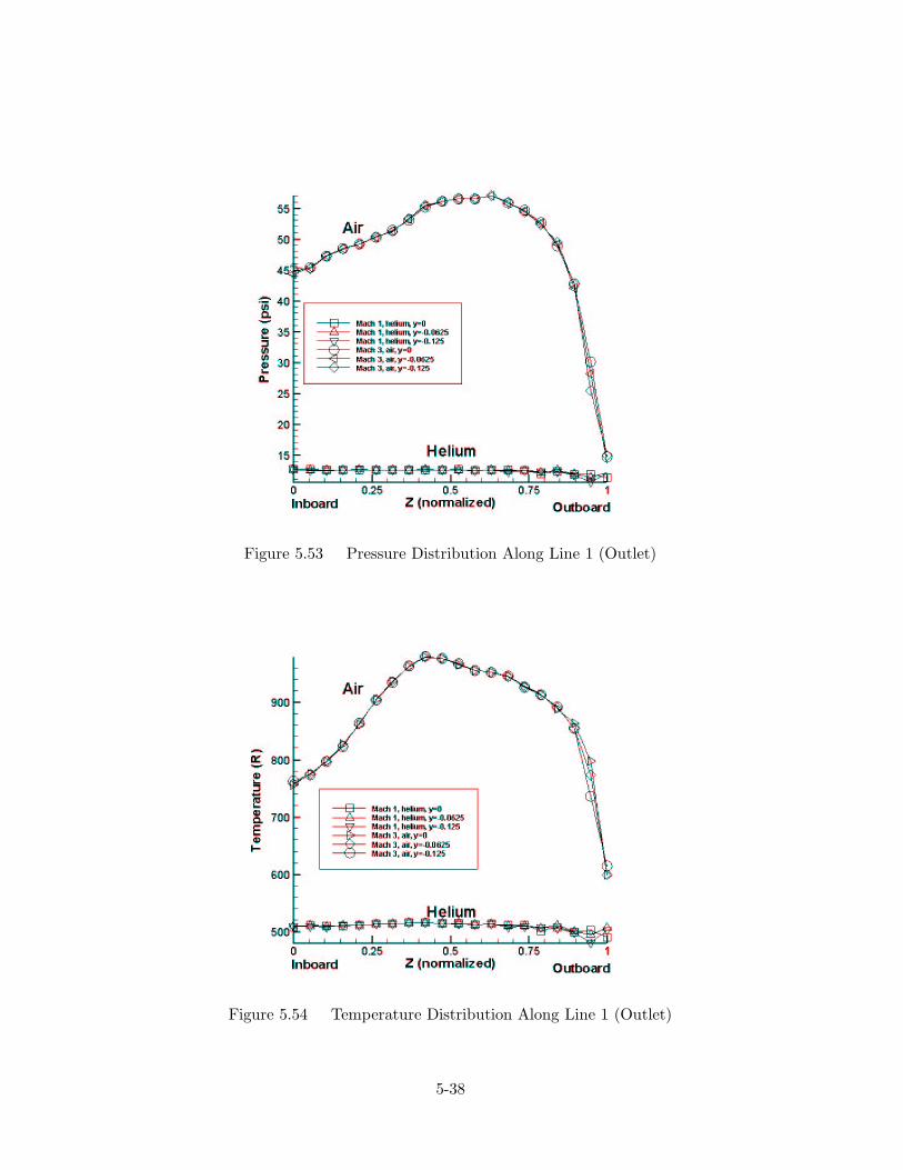
Figure 5.53 Pressure Distribution Along Line 1 (Outlet)

Figure 5.54 Temperature Distribution Along Line 1 (Outlet)

5-38

Figure 5.55 Pressure Distribution Along Line 2 (Inboard Side)

Figure 5.56 Temperature Distribution Along Line 2 (Inboard Side)

5-39

Figure 5.57 Pressure Distribution Along Line 3 (Outboard Side)

Figure 5.58 Temperature Distribution Along Line 3 (Outboard Side)

5-40

Unsteady, Inviscid Flow

Due to the vast amount of data generated with the unsteady computation and the

difficulty in visualizing the results on paper, only the pressure solution will be presented

here, although the same trends occur for the temperature and density values.

A total of 7.5 milliseconds were modeled with the unsteady calculation, with 1,500

time steps (∆t = 5 × 10−6 seconds). Snapshots of the solution were taken every 200 time

steps, generating 750 animation frames. Of those 750, nine are presented here.

As discussed previously, the unsteady computation was set up by simply changing the

boundary condition on the pressure-far-field boundary to be 100% helium at M∞ = 1.02,

or 3,300 fps. Figures 5.59-5.62 show the mass fraction of air during a portion of the

computation. The helium diffuses through the domain within a period of 5 milliseconds.

It should be noted that the surface boundaries still reflect a composition of 100% air due to

the way the boundary conditions are implemented in FLUENT. Several different methods

of implementing the boundary conditions were explored, but all gave the same results.

These frames illustrate a difficulty with modeling the unsteady transition from air

to helium as the sled enters a tent. Presumably, the transition should take place in a

constant-x plane – that is, the helium should diffuse from upstream of the sled only.

However, due to the shape of the pressure-far-field boundary, helium was introduced into

the domain as a function of x also (it appears as though the helium were diffusing in from

the zmax boundary as well). Although this may not be entirely accurate, the sled is engulfed

completely in the helium environment in less than 2 milliseconds and the inaccuracies may

be negligible. The simulation would most likely be more accurate if different boundary

zones were implemented to model the transition better.

5-41

Figure 5.59 Mass Fraction of Air at t = 1.0 × 10−3 Seconds

Figure 5.60 Mass Fraction of Air at t = 2.0 × 10−3 Seconds

5-42

Figure 5.61 Mass Fraction of Air at t = 3.0e − 3 Seconds

Figure 5.62 Mass Fraction of Air at t = 4.0e − 3 Seconds

5-43

Figure 5.63 Drag Coefficient During Air-to-Helium Transition

The drag coefficient changes during the air-to-helium transition is shown in Fig-

ure 5.63. As the sled begins to enter the helium at about 2 milliseconds, the drag coeffi-

cient drops. The entire sled is engulfed in helium a little before 4 milliseconds. The slight

bounce in the drag coefficient as it bottoms out, begins to increase, then decreases again

demonstrates the dynamic effect as the pressures stabilize after the sled has completely

entered the helium environment. The unsteadiness eventually settles out to a steady-state

solution after 6 milliseconds.

Figures 5.64-5.81 give a good idea of the pressure distribution throughout the transi-

tion. These frames span the time from t = 2.0× 10−3 to t = 6.0× 10−3. It is important to

note that the range of pressure contours are different for each frame; the optimal contour

level range was computed automatically by Tecplot to give the best resolution of contours

at each time step.

During the transition, the maximum pressures decrease and the shock angles increase,

giving the appearance that the contours ”spread out” (that is, the shocks don’t lay so

closely to the sled itself, but fan out into the freestream). The dynamic effect seen in the

5-44

Figure 5.64 Static Pressure (psi) Contours at t = 2.0 × 10−3 Seconds

drag coefficient is also seen in the pressure contours as the Mach line extending upward

from the expansion around the shoulder of the vertical wedge continues to come forward

(Figure 5.69) and then settles further back on the body (Figure 5.72).

These frames also show that the maximum pressure areas migrate from the corner

near the slipper wedge (where the shock impinges on the structure) and settles on the

stagnation region on the leading edge of the wedges. The final steady-state solution is the

familiar solution discussed previously for the M∞ = 1.02 in helium case.

5-45



5-46



5-47


Figure 5.70 Static Pressure (psi) Contours at t = 4.5 × 103 Seconds

5-48



5-49

Figure 5.73 Surface Static Pressure (psi) Contours at t = 2.0 × 10−3 Seconds

The pressure on the underside of the slipper wedge (upper surface of the slipper

wedge/rail gap) is seen in Figures 5.73-5.81. The gradients change from those caused by

the impinging shock, to those resulting from the flow stagnation on the leading edge of the

wedge.

When viewing the animations from which these frames where taken, some unsteadi-

ness was observed on the underside of the strut wedge at the outflow plane. Oscillations in

the pressure gradients were observed in this area toward the end of the unsteady flow sim-

ulations, that is, after the solutions was to have achieved a steady state. This suggests one

of two things; either the boundary conditions are influencing the solution in non-physical

ways, or there is an inherent unsteadiness in the flow at that point. These oscillations were

not observed at any other location in the domain, suggesting that it is, in fact, an inher-

ent unsteadiness. This could explain the oscillations in the residual values that prevented

the reduction in residuals by three orders of magnitudes. Similar unsteadiness may have

caused the second-order solutions to become unstable as well (the numerical viscosity in

first-order solutions may have damped out the oscillations).

5-50



5-51



5-52



5-53



5-54

VI. Conclusions and Recommendations

Steady, three-dimensional, inviscid flow solutions were presented for Mach numbers of 2

and 3 in air (2,200 and 3,300 feet per second), and for Mach numbers of 1.02, 2.5 and 3.1

in helium (3,300, 8,076 and 10,000 feet per second). Second-order solutions were obtained

for the Mach 3 in air and Mach 1.02 in helium cases. The unsteady transition from air to

helium at 3,300 feet per second was also modeled.

Mesh adaptation allows the computation of accurate CFD solutions while maintain-

ing computational efficiency. The adaptation procedure, based on gradients of pressure,

is an effective method to refine the flow solution in regions around shock waves and were

utilized in this study. The resulting meshes contained around 2 million cells, dramatically

increasing the memory and computation requirements.

Mesh quality can also impact the stability and accuracy of the solution. Node spac-

ings in the slipper/rail gap region may not have been sufficiently small; mesh adaptations

improved this to some extent. Second-order results were obtained for the M∞ = 3.0 in air

and M∞ = 1.02 in helium cases, while only first-order results were obtained for the other

cases modeled.

The thermodynamic properties of the flow around the hypervelocity sled are strongly

affected by the discontinuities of the flow, such as shock waves, expansions and their

interactions. In turn, the location of these shocks and expansions are dependent on the

Mach number of the freestream (or velocity of the sled).

In the case of the M∞ = 3.0 flow in air, the shock generated by the vertical wedge

impinges on the sled structure. The resulting reflection and interaction with other flow

features and structural components create a stagnation region with high temperatures and

pressures. These high temperatures and pressures could weaken the structure, decreasing

the performance of the sled. Additionally, the high gradients could cause vibrations and

heating that would worsen damage through the gouging phenomenon.

The same deteriorating effects are not seen in the M∞ = 1.02 in helium case, even

though the actual velocities are the same. The magnitudes of the pressures and temper-

6-1

atures are reduced, with the maximum values being in the stagnation regions along the

leading edges of the wedges.

The flow entering the slipper/rail gap is also strongly affected by the location of any

shocks in the flow. Again, the aero-thermodynamic heating is reduced in the gap area

when run through a helium rather than an air environment.

Future Work

The research presented here is only the beginning of what would need to be accom-

plished to accurately model the flow around the hypervelocity sled. Some of those areas

that need future work include:

• Improvements in mesh generation. The existing mesh was shown to be of

fairly low quality. This may have had an impact on the stability and accuracy of the

solution. A suggested method to investigate the effects of mesh quality on the solution

stability is to gradually build up the model from component pieces. One could start

with the payload section and compute the relatively simple solution (including a

second-order solution to verify stability) about that section only. Other components

could then be added. In this way, areas of the mesh that affect solution stability can

be found and improved.

• Second-order solutions for all cases. The stability and convergence properties

of the second-order solver is much more sensitive than the first-order solver. Refining

the mesh generation process may solve this problem.

• Mesh adaptation. The type of mesh adaptation discussed here (conformal node

adaptation based on pressure gradients) is only a small portion of what is available in

FLUENT. The main constraint on adaptation was due to memory limits; conformal

node adaptation can only be performed on a single processor. Another method, the

hanging-node method, while using more memory, can be performed in parallel. With

more machines available, the memory constraints would not be as restrictive and the

maximum gradients can be reduced further.

6-2

• Viscous effects. The actual aerodynamic heating that occurs as the shocks impinge

on the structural components of the sled cannot be predicted without accurately

modeling the viscous effects. Neither can the flow field properties be accurately

modeled in the slipper/rail gap, where the boundary layer thickness may be close to

the gap height. The work involved in the construction of a viscous mesh and the

subsequent numerical solutions is at least an order of magnitude greater than the

work in this study.

• Modeling of the actual slipper/rail gap. The current model was truncated

forward of the actual slipper/rail gap due to numerical concerns. If the sled is modeled

using a fully viscous model, these issues would no longer be of concern.

• Pseudo-Unsteady Solutions. The current study showed that there may be in-

herent unsteadiness in the flow. This unsteadiness would possibly prevent a steady

solution from converging. Computing a steady solution with an unsteady scheme

would capture the steady solution without the convergence difficulties.

6-3

Bibliography

1. Amtec Engineering Incorporated, Bellevue WA. CFD Analyzer User’s Manual, Version

2.0 , 1999. Electronic documentation, http://www.amtec.com.

2. Amtec Engineering Incorporated, Bellevue WA. Tecplot User’s Manual, Version 9,

Revision 2 , August 2001.

3. Bosmajian, Neil and others. Status of the Magnetic Levitation Upgrade of the Holloman

High Speed Test Track . AIAA Technical Paper AIAA-2000-2289, Washington DC:American Institute of Aeronautics and Astronautics, 2000.

4. Fluent Incorporated, Lebanon NH. Fluent 6.0 User’s Guide, December 2001. Elec-tronic documentation on CD-ROM accompanying FLUENT Version 6.0 software.

5. Guide for the Verification and Validation of Computational Fluid Dynamics Simula-

tions. AIAA Guide G-077-1998, Washington DC: American Institute of Aeronauticsand Astronautics, January 1998.

6. Hoffmann, Klaus A. and Steve T. Chiang. Computational Fluid Dynamics (FourthEdition), Volume II . Wichita KS: Engineering Education System, August 2000.

7. Hoffmann, Klaus A. and Steve T. Chiang. Computational Fluid Dynamics (FourthEdition), Volume I . Wichita KS: Engineering Education System, August 2000.

8. Hooser, Michael. Simulation of a 10,000 Foot per Second Ground Vehicle. AIAATechnical Paper AIAA-2000-2290, Washington DC: American Institute of Aeronauticsand Astronautics, 2000.

9. Hooser, Michael D. Personal Correspondance. Holloman Air Force Base NM: 846TS/TGTDD, 2001.

10. Jenke, Leroy M. and Ernest J. Lucas. Supersonic Wind Tunnel Tests of Dual Rail and

Monorail Rocket Sleds. Technical Report AEDC-TR-65-70, Arnold Air Force StationTN: Arnold Engineering Development Center, April 1965.

11. Korkegi, Robert H. and Ronald A. Briggs. Aerodynamics of the Hypersonic Slip-

per Bearing . Technical Report ARL 68-0028, Wright-Patterson Air Force Base OH:Aerospace Research Laboratories, February 1968.

12. Korkegi, Robert H. and Ronald A. Briggs. “The Hypersonic Slipper Bearing–A TestTrack Problem,” Journal of Spacecraft and Rockets, 6 (2):210–212 (February 1969).

13. Krupovage, Daniel J. and Hans J. Rassmussen. Hypersonic Rocket Sled Development .Technical Report AD-TR-82-41, Holloman Air Force Base NM: Test Track Division,September 1982.

14. Laird, David J. The Investigation of Hypervelocity Gouging . PhD dissertation,Graduate School of Engineering, Air Force Institute of Technology (AETC), Wright-Patterson AFB OH, January 2002 (AFIT/DS/ENY/02-01).

15. Myers, Jack. “Aerodynamic Analysis, Nike O/U Narrow Gage Sled, Generic Payload.”Unpublished Draft Report, Personal Communication, February 2002.

BIB-1

16. National Advisory Committee for Aeronautics (NACA). Equations, Tables and Charts

for Compressible Flow . Report 1135. Moffett Field CA: Ames Aeronautical Laboratory,1953.

17. Pointwise, Incorporated, Fort Worth TX. Gridgen User Manual, Version 13.3 , 1999.Electronic documentation on CD-ROM accompanying Gridgen Version 13.3 software.

18. Roache, Patrick J. Verification and Validation in Computational Science and Engi-

neering . Albuquerque NM: Hermosa Publishers, 1998.

19. Schoenfeld, William P. Requirements for Upgrading the Holloman High Speed Test

Track Computational Fluid Dynamics Analytical Capability . AIAA Technical PaperAIAA-2000-2288, Washington DC: American Institute of Aeronautics and Astronau-tics, 2000.

20. Thompson, Joe F., “A Reflection on Grid Generation in the 90s: Trends, Needsand Influences.” http://capella.colorado.edu/~laney/thompson.htm, 12 Decem-ber 2001.

21. U.S. Government Printing Office. U.S. Standard Atmosphere, 1976 . Technical Report.1976. http://aero.stanford.edu/StdAtm.html.

22. Warren, Gary P. and others. Grid Convergence for Adaptive Methods. AIAA Tech-nical Paper AIAA-91-1591, Washington, DC: American Institute of Aeronautics andAstronautics, 1991.

BIB-2

Vita

Captain Andrew J. Lofthouse graduated from Timpview High School in Provo, Utah,

in 1991. Following graduation, he enlisted in the United States Air Force Reserves as an

Aircraft Armament Systems Specialist with the 419th Tactical Fighter Wing, Hill Air

Force Base, Utah. He entered undergraduate studies at Brigham Young University in

Provo, Utah where he graduated with a degree in Mechanical Engineering in December of

1997. He was commissioned as a Second Lieutenant in the United States Air Force through

Detachment 855 of AFROTC at Brigham Young University where he was recognized as a

distinguished graduate.

His first assignment was to the Warner Robins Air Logistics Center at Robins AFB,

Georgia as an Aircraft Battle Damage Repair Engineer and a program manager. In Septem-

ber 2000, he was assigned to Wright-Patterson AFB, Ohio as a graduate student in the

Aeronautical Engineering program at the Air Force Institute of Technology. Upon gradua-

tion, he will be assigned to the National Air Intelligence Center at Wright-Patterson AFB,

Ohio.

VITA-1

REPORT DOCUMENTATION PAGE Form Approved OMB No. 074-0188

The public reporting burden for this collection of information is estimated to average 1 hour per response, including the time for reviewing instructions, searching existing data sources, gathering and maintaining the data needed, and completing and reviewing the collection of information. Send comments regarding this burden estimate or any other aspect of the collection of information, including suggestions for reducing this burden to Department of Defense, Washington Headquarters Services, Directorate for Information Operations and Reports (0704-0188), 1215 Jefferson Davis Highway, Suite 1204, Arlington, VA 22202-4302. Respondents should be aware that notwithstanding any other provision of law, no person shall be subject to an penalty for failing to comply with a collection of information if it does not display a currently valid OMB control number. PLEASE DO NOT RETURN YOUR FORM TO THE ABOVE ADDRESS. 1. REPORT DATE (DD-MM-YYYY)

26-03-2002 2. REPORT TYPE Master’s Thesis

3. DATES COVERED (From – To)

Sep 2001 – Mar 2002 5a. CONTRACT NUMBER

5b. GRANT NUMBER

4. TITLE AND SUBTITLE COMPUTATIONAL AERODYNAMIC ANALYSIS OF THE FLOW FIELD ABOUT A HYPERVELOCITY TEST SLED 5c. PROGRAM ELEMENT NUMBER

5d. PROJECT NUMBER ENR# 1999-115

5e. TASK NUMBER

6. AUTHOR(S) Lofthouse, Andrew J., Capt, USAF

5f. WORK UNIT NUMBER

7. PERFORMING ORGANIZATION NAMES(S) AND ADDRESS(S) Air Force Institute of Technology Graduate School of Engineering and Management (AFIT/ENY) 2950 P Street, Building 640 WPAFB OH 45433-7765

8. PERFORMING ORGANIZATION REPORT NUMBER

AFIT/GAE/ENY/02-07

10. SPONSOR/MONITOR’S ACRONYM(S)

9. SPONSORING/MONITORING AGENCY NAME(S) AND ADDRESS(ES) AFOSR/NM Attn: Dr. Len Sakell 801 N. Randolph Street, Romm 732 Arlington, VA 22203-1977 DSN: 426-6566

11. SPONSOR/MONITOR’S REPORT NUMBER(S)

12. DISTRIBUTION/AVAILABILITY STATEMENT APPROVED FOR PUBLIC RELEASE; DISTRIBUTION UNLIMITED.

13. SUPPLEMENTARY NOTES

.

14. ABSTRACT The flow field about the nose section of a hypervelocity test sled is computed using computational fluid dynamics. The numerical model of the test sled corresponds to the Nike O/U narrow gage sled used in the upgrade program at the High Speed Test Track facility, Holloman Air Force Base, New Mexico. The high temperatures and pressures resulting from the aerodynamic heating and loading affect the sled structure and the performance of the vehicle. The sled transitions from an air environment to a helium environment at a speed of approximately 3,300 feet per second (Mach 3 in air, Mach 1.02 in helium) to reduce the effects of high Mach number flows. Steady, three-dimensional, inviscid flow solutions are computed for Mach numbers of 2 and 3 in air (2,200 and 3,300 feet per second), and for Mach numbers of 1.02, 2.5 and 3.1 in helium (3,300, 8,076 and 10,000 feet per second). Mesh adaptation is used to obtain a mesh-independent solution. Second-order solutions are obtained for the Mach 3 in air and Mach 1.02 in helium cases. The unsteady transition from air to helium at 3,300 feet per second is also modeled. Mach 3 in air computations are compared with analytical results. 15. SUBJECT TERMS

High Velocity, Test Vehicles, Computational Fluid Dynamics, Hypersonic Test Vehicles, Euler Equations

16. SECURITY CLASSIFICATION OF: 19a. NAME OF RESPONSIBLE PERSON Lt Col Montgomery C. Hughson

a. REPORT

U b. ABSTRACT

U c. THIS PAGE

U

17. LIMITATION OF ABSTRACT

UU

18. NUMBER OF PAGES

118 19b. TELEPHONE NUMBER (Include area code)

(937) 255-3636 ext 4597 Standard Form 298 (Rev. 8-98)

Prescribed by ANSI Std. Z39-18

Form Approved OMB No. 074-0188

flow over aircraft

Documents

united states air force

holloman air force base

flow solution

flow field

computational time

mesh generation

computational facilities3

equations of fluid flow