fluent ic tut 09 inert

Tutorial: EGR Modeling Using the Inert Model

Introduction

Exhaust gas recirculation (EGR) is, among other things, a NOx emissions reduction tech-nique used in most gasoline and diesel engines. EGR works by recirculating a portion of theexhaust gas of an engine back to the engine cylinders. Intermixing the incoming air withrecirculated exhaust gas dilutes the mix with inert gas. It lowers the adiabatic flame tem-perature and (in diesel engines) reduces the amount of excess oxygen. The exhaust gas alsoincreases the specific heat capacity of the mix lowering the peak combustion temperature.NOx formation progresses much faster at high temperatures. Hence, EGR helps in limitingthe generation of NOx. NOx is primarily formed when a mix of nitrogen and oxygen issubjected to high temperatures.

Modeling Combustion with EGR

If only combustion process is modeled, namely from Intake Valve Close (IVC) to ExhaustValve Open (EVO), there are two ways of modeling EGR inside ANSYS FLUENT. Theconventional way is to use non-premixed combustion model of ANSYS FLUENT with theEGR species included in the oxidizer stream.

ANSYS FLUENT has an inert model, which can be used to model EGR or residual gas. Theinert model treats the EGR as if it does not participate in any combustion. Even though theconventional way should be more accurate since the EGR is in the equilibrium calculation,inert treatment offers some advantages for EGR modeling. If intake stroke is included aspart of the simulation, the conventional way will not be applicable since the EGR comesin a separate stream and thus can not be included as part of the oxidizer stream. In suchcases, the two mixture fraction approach is desired to obtain full equilibrium of EGR. Butit is a very expensive process. However, if full equilibrium can be relaxed, the inert optionis a much less expensive option for modeling EGR.

Prerequisites

This tutorial is written with the assumption that you have completed Tutorial 1 fromANSYS FLUENT 13.0 Tutorial Guide, and that you are familiar with the ANSYS FLUENTnavigation pane and menu structure. Some steps in the setup and solution procedure willnot be shown explicitly.

Problem Description

A 30 degree periodic slice of the piston-cylinder combination is considered in this problem.This simulation starts at intake valve close (IVC) and ends at exhaust valve open (EVO).

c© ANSYS, Inc. October 12, 2010 1


So, there are no valves involved, and only the compression and power stroke is simulated.A pure layering approach is used on a 3D sector mesh. The problem schematic showsthe geometry and the problem domain used. Methane is used as the fuel and that entersthrough the inlet. The flow rate of methane is specified in the UDF.

The tutorial demonstrates the following:

• Setting up a CIC case involving only compression and power stroke with only a sectorof mesh.

• Setting up EGR combustion using inert model in ANSYS FLUENT. A 12% EGR-airmixture is used in the tutorial.

Figure 1: Problem Schematic

2 c© ANSYS, Inc. October 12, 2010


Setup and Solution

Preparation

1. Copy the files, egr tut.msh.gz, initialize.c, and injection ch4.c to your work-ing folder.

2. Use FLUENT Launcher to start the 3D version of ANSYS FLUENT.

For more information about FLUENT Launcher refer to section 1.1.2 in the FLUENT13.0 User’s Guide.

3. Enable Double-Precision in the Display Options list.

4. Click the UDF Compiler tab and ensure that Setup Compilation Environment for UDFis enabled.

The path to the .bat file which is required to compile the UDF will be displayed assoon as you enable Setup Compilation Environment for UDF.

If the UDF Compiler tab does not appear in the FLUENT Launcher dialog box by default,click the Show Additional Options>> button to view the additional settings.

Note: The Display Options are enabled by default. Therefore, after you read in themesh, it will be displayed in the embedded graphics window.

Step 1: Mesh

1. Read the mesh file (egr tut.msh.gz).

File −→ Read −→Mesh...

As ANSYS FLUENT reads the mesh file, messages will appear in the console reportingthe progress of the conversion.

Note: There is only 30 degrees of the mesh, which is corresponding to one fuel injector hole.The piston is at the top dead center (TDC), the recommended location of meshing forinternal combustion (IC) simulations. This is because the squish volume is minimumat this piston position. If mesh is built correctly in this position, it is easy to ensurethat the mesh motion will succeed for the whole engine cycle. Later, the mesh willbe moved to IVC position, the starting point of simulation. In convention of ANSYSFLUENT, TDC after compression stroke is 0. Crank angle (CA) and TDC afterexhaust stroke is 360 CA.



Figure 2: Mesh Display

Step 2: General Settings

1. Select the transient solver.

General −→ Transient

2. Check the mesh.

General −→ Check

ANSYS FLUENT will perform various checks on the mesh and report the progress inthe console. Ensure that the minimum volume reported is a positive number.

Warnings will be displayed regarding unassigned interface zones, resulting in the failureof the mesh check. You do not need to take any action at this point, as this issue willbe rectified when you define the mesh interfaces in a later step.



3. Scale the mesh.

General −→ Scale...

(a) Retain the default settings as the grid is already scaled.

Make sure the scale parameters in the Scale Mesh dialog box are same as thatshown.

(b) Close the Scale Mesh dialog box.

4. Compile and load the user-defined functions (UDF).

Define −→ User-Defined −→ Functions −→Compiled...

(a) Click Add... in the Source Files group box.

The Select File dialog box will open.

i. Select the files, initialize.c and injection ch4.c and click OK.

(b) Click Build in the Compiled UDFs dialog box.

Here you will create a library with the default name of function::libudf inyour working folder. If you would like to use a different name, you can enter itin the Library Name field. In this case you need to ensure that you will open thecorrect library in the next step.

A dialog box will appear warning you to ensure that the UDF source files are inthe folder that contains your case and data files. Click OK in the warning dialogbox.

(c) Click Load to load the UDF library you just compiled.

When the UDF is built and loaded, it is available to hook to your model. It(function::libudf) can be selected from drop-down lists of various dialog boxes.

The user-defined functions will be used to initialize the solution and to provide thefuel injection correctly. Refer the Appendix B for more details about the UDFs.



5. Hook the UDF library

Define −→ User-Defined −→Functions Hooks...

(a) Click Edit... for Initialization.

(b) Select my init funcation::libudf in Available Initialization Functions and clickAdd.

(c) Click OK to close the Initialization Functions dialog box.

(d) Click OK to close the User-Defined Function Hooks dialog box.

6. Create periodic boundary out of face zone period inner1 and period inner2. Use thetext command as shown.

/mesh/modify-zones>make-periodic

Periodic zone[()] period_inner1

Shawdow zone[()] period_inner2

Rotational periodic? (if no, translational)[yes] yes

Create periodic zones? [yes] yes

all 700 faces matched for zones 12 and 11.

zone 11 deletedcreated periodic zones.

7. Similarly create another periodic boundary using the face zones period outer1 andperiod outer2.

Step 3: Models

1. Enable the Energy Equation.

Models −→ Energy −→ Edit...

(a) Enable the Energy Equation.

(b) Click OK to close the Energy dialog box.

2. Enable the standard k-ε turbulence model.

Models −→ Viscous −→ Edit...

(a) Select k-epsilon (2 eqn) in the Model list.

The original Viscous Model dialog box will expand when you do so.

(b) Click OK to accept the default Standard model and close the Viscous Model dialogbox.



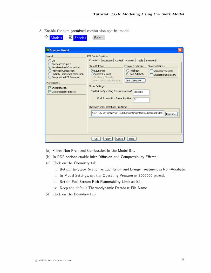
3. Enable the non-premixed combustion species model.

Models −→ Species −→ Edit...

(a) Select Non-Premixed Combustion in the Model list.

(b) In PDF options enable Inlet Diffusion and Compressibility Effects.

(c) Click on the Chemistry tab.

i. Retain the State Relation as Equilibrium and Energy Treatment as Non-Adiabatic.

ii. In Model Settings, set the Operating Pressure as 3000000 pascal.

iii. Retain Fuel Stream Rich Flammability Limit as 0.1.

iv. Keep the default Thermodynamic Database File Name.

(d) Click on the Boundary tab.



By default ch4, h2, jet-a<g>, n2, o2 species will be present.

i. Select Mole Fraction from the Specify Species in group box.

ii. Type h2o in the Boundary Species text box and click Add.

iii. Similarly, add co and co2 species.

iv. Enter Fuel value of ch4 as 1.

(e) Click on the Table tab.

i. Retain the default settings in Table Parameters group box.

ii. Click Calculate PDF Table.

ANSYS FLUENT will take some time to generate the PDF table. You canpreview the PDF table by clicking on Display PDF Table... button.

iii. Click Apply.

iv. Click OK to close the Species Model dialog box.

4. Save the PDF file.

File −→ Write −→PDF...

(a) Enter natural gas EGR inert.pdf.gz for the file name.

(b) Click OK to close the Select File dialog box.



5. Enable the Inert Transport model.

Models (Species - Non-Premixed Combustion)−→ Inert −→ Edit...

(a) Select Inert Transport.

(b) Select User Specified in Composition Options group box.

By default the species will consist of co2, h2o, and n2.

(c) In the Inert Species text box, type ch4 and click Add.

(d) Similarly, add o2, h2, and co Inert Species to the Species list.

(e) Set the Mass Fraction of each Species as shown in the table.

Species Mass Fractionco2 0.08933h2o 0.08402n2 0.72916ch4 0.00131o2 0.06649h2 0.00267co 0.02702

(f) Click OK to close the Inert dialog box.

Step 4: Materials

Materials

You can find that a pdf-mixture species is defined under Materials.

Retain the default material properties.



Step 5: Cell Zone Conditions

Cell Zone Conditions

You can find three cell zones, fluid-inj, fluid-inner, and fluid-outer.

Retain the default Cell Zone Conditions.

Step 6: Boundary Conditions

Boundary Conditions

1. Set the boundary conditions at inlet.

Boundary Conditions −→ inlet −→ Edit...

(a) Select Mass Flux from the Mass Flow Specification Method drop-down list in theMomentum tab.

(b) Select udf fuel flux::libudf from the Mass Flux drop-down list.

(c) Select Normal to Boundary from the the Direction Specification Method.

(d) Select Intensity and Length Scale from the Specification Method drop-down list inthe Turbulence group box.

(e) Retain 10% for Turbulence Intensity

(f) Enter 2 mm for Turbulent Length Scale.

(g) Click Thermal tab and ensure Total Temperature is set to 300 K.

(h) In the Species tab, specify a Mean Mixture Fraction of 1.



(i) Click OK to close the Mass-Flow Inlet dialog box.

2. Ensure that the period inner1 and the period outer1 zone type is rotational.

(a) Ensure that period inner1 zone type is set to rotational.

Boundary Conditions −→ period inner1 −→ Edit...

(b) Similarly check that period outer1 is set to rotational.

Boundary Conditions −→ period outer1 −→ Edit...

Step 7: Mesh Interface Setup

Mesh Interfaces −→ Create/Edit...

1. Enter interface for the Mesh Interface name.

2. Select intf-inner as Interface Zone 1 and intf-outer as Interface Zone 2.

3. Click Create and close the Create/Edit Mesh Interfaces dialog box.

4. Perform a mesh check.

General −→ Check

In the mesh check report, the angle of periodic boundaries is reported as 30 degrees.



Step 8: Dynamic Mesh Setup

Dynamic Mesh

1. Enable Dynamic Mesh in the Dynamic Mesh task page.

2. Disable Smoothing and enable Layering option in the Mesh Methods group box.

ANSYS FLUENT will automatically flag the existing mesh zones for use of the differentdynamic mesh methods where applicable

3. Click Settings... to open the Mesh Method Settings dialog box.



(a) Click the Layering tab.

(b) Select Ratio Based in the Options group box.

(c) Retain 0.4 for Split Factor.

(d) Enter 0.1 for Collapse Factor.

(e) Click OK to close the Mesh Method Settings dialog box.



4. Enable In-Cylinder and click Settings... in the Options group box.

(a) Enter 700 degrees for Starting Crank Angle.

(b) Enter 0.25 degrees for Crank Angle Step Size.

(c) Enter 120 mm for Piston Stroke and 220 mm for Connecting Rod Length.

(d) Click OK to save the parameters and close the In-Cylinder Settings dialog box.



5. Define dynamic mesh zones to simulate the moving mesh.

Dynamic Mesh (Dynamic Mesh Zones)−→ Create/Edit...

(a) Ensure that bowl is selected from the Zone Names.

(b) Ensure that the Type selected is Rigid Body.

(c) In Motion Attributes tab, ensure that **piston-full** is selected as the MotionUDF/Profile.

(d) Enter 0 for X axis and 1 for Z axis in the Valve/Piston Axis group box.

(e) In the Meshing Options tab ensure that Cell Height is set to 0.

(f) Click Create.

(g) Similarly, for bowl:17 zone retain the other options and enter 1 mm for Cell Heightin Meshing Options tab.

(h) Click Create.

(i) Select fluid-outer in Zone Names and click Create.

(j) For wall top outer, select Type as Stationary and in Meshing Options tab, enter1.2 mm for Cell Height and click Create.

(k) Close the Dynamic Mesh Zones dialog box.



6. Save the case file (natural gas EGR inert.cas.gz).

File −→ Write −→Case...

• Preview the zone motion to check the correctness of the motions specified byclicking the Display Zone Motion... button.

• Preview the mesh motion to check the correctness of dynamic mesh set up byclicking the Display Mesh Motion... button. Save the case file before previewingthe mesh motion.

• Read the saved case file, (natural gas EGR inert.cas.gz) if you have previewdmesh motion before proceeding to the next steps.

File −→ Read −→Case...

Note: The whole fluid zone and piston will move up and down using a profile (**piston-full**), generated automatically by ANSYS FLUENT using crank radius and con-necting rod length. The cylinder head (wall top outer) is stationary. Relativemotion is detected at the cylinder head and hence layers are added and deletedat this zone. Similarly, layers are added and deleted at the zone, bowl:017.



Step 9: Solution

1. Set solution parameters.

Solution Methods

(a) Select PISO from the Scheme drop-down list in the Pressure-Velocity Couplinggroup box.

(b) Set 0 for Skewness Correction.

(c) Retain 1 for Neighbor Correction.

(d) Ensure that Skewness-Neighbor Coupling is enabled.

(e) Select Second Order Upwind from Momentum drop-down list in Spatial Discretiza-tion group box.

2. Set the relaxation factors.

Solution Controls

(a) Enter 0.5 for Pressure in the Under-Relaxation Factors group box.

(b) Enter 0.99 for Energy.



3. Enable the plotting of residuals during calculation.

Monitors −→ Residuals −→ Edit...

(a) Ensure that Plot is enabled.

(b) Disable Check Convergence for continuity in the Equations group box.

(c) Click OK to close the Residual Monitors dialog box.

4. Enable the plotting of mass flow rate at inlet.

Monitors (Surface Monitors)−→ Create...

(a) Enable Plot and ensure that Window is set to 2.

(b) Enable Write and enter ./mass flow rate inlet.out for File Name.

(c) Select Flow Time from X-Axis drop-down list.

(d) Select Time-Step from Get Data Every drop-down list.

(e) Select Mass Flow Rate from Report Type drop-down list.

(f) Select inlet from the list of Surfaces.

(g) Click OK to close the Surface Monitor dialog box.



5. Enable the plotting of mass-weighted-average of static temperature.

Monitors (Volume Monitors)−→ Create...


(b) Enable Write and enter ./vol temp.out for File Name.



(e) Select Mass-Average from Report Type drop-down list.

(f) Select Temperature... and Static Temperature from Field Variable drop-down lists.

(g) Select fluid-outer and fluid-inner from Cell Zones lists.

(h) Click OK to close the Volume Monitor dialog box.

6. Enable the plotting of volume-weighted-average of static pressure.

Monitors (Volume Monitors)−→ Create...


(b) Enable Write and enter ./vol pressure.out for File Name.



(e) Select Volume-Average from Report Type drop-down list.

(f) Ensure that Pressure... and Static Pressure are selected from Field Variable drop-down lists.

(g) From Cell Zones select fluid-outer and fluid-inner.

(h) Click OK to close the Volume Monitor dialog box.



7. Initialize the solution.

Solution Initialization

(a) Enter 1898675 pascal for Gauge Pressure.

(b) Enter 690 K for Temperature.

(c) Enter 0.12 for Inert Variable.

(d) Click Initialize.

Note: The initial values are calculated based on the isentropic relationship as-suming ideal gas. Initial conditions of fluid are assumed to be at STP.

P1 = 101325PaT1 = 300Kgamma = 1.365Compression ratio(CR) = 11.42(V2/V1) at CA 700 = 8.689 (using geometry analysis)P1V1gamma = P2V2gamma

P2 = 1898675PaT1V1(gamma−1) = T2V2(gamma−1)

T2 = 690K

8. Start the calculation.

Calculation Activities

(a) Enter 50 for Autosave Every (Time Steps).

(b) Click Edit....

(c) Enter natural gas EGR inert-CA700.gz for the File Name.

(d) Click OK to close the Autosave dialog box.



9. Create an iso-surface.

Before specifying the commands to save the solution images at regular intervals, weneed to define a postprocessing surface and a postprocessing view.

Surface −→Iso-Surface...

(a) Select Mesh... and Angular Coordinate from Surface of Constant drop-down lists.

(b) Enter 75 degrees for Iso-Values.

(c) Enter theta=75 for New Surface Name.

(d) Click Compute and then Create.

(e) Close the Iso-Surface dialog box.

10. Display the new surface.

Graphics and Animations (Graphics)−→ Mesh −→ Set Up...

(a) Deselect all the Surfaces.

(b) Select theta=75 and click Display.

(c) Orient the display as shown in Figure 3.

(d) Close the Mesh Display dialog box.



Figure 3: Iso-Surface Mesh Display

11. Create a post processing view.

Graphics and Animations −→ Views

(a) Enter plot-view for Save Name.

(b) Click Save and close the Views dialog box.



12. Specify the commands to save the solution images at regular intervals.

Calculation Activities (Execute Commands)−→ Create/Edit...

(a) Set the Defined Commands to 4.

(b) Enable Active for all 4 commands.

(c) Set Every for all commands to 10.

(d) Select Time Step from the When drop-down lists for all commands.

(e) Enter the commands as shown in the table.

Name Command

command-1 /dis/sw 5 /dis/view/rv plot-view /dis/set/cont/sur(theta=75) /dis/cont ch4 0 1

command-2 dis/save-p ch4-%t.tif ycommand-3 /dis/sw 4 /dis/view/rv plot-view /dis/set/cont/sur

(theta=75) /dis/cont temp 600 2500command-4 /dis/save-p temp-%t.tif y

(f) Click OK to close the Execute Commands dialog box.

13. Save the case and data file (natural gas EGR inert-CA700.cas.gz).

File −→ Write −→Case & Data...

14. Run calculation for 400 time steps.

Run Calculation

(a) Enter 400 for Number of Time Steps.

(b) Click Calculate.



Step 8: Postprocessing

1. Plot the pressure curves.

Plots −→ File −→ Set Up...

(a) Click Add... in the File XY Plot dialog box.

(b) Select vol pressure.out.

(c) Click OK to close the Select File dialog box.

(d) Click Plot.

Figure 4: Pressure Variation Inside The Cylinder

2. Plot the temperature curves.

Plots −→ File −→ Set Up...

(a) Click Delete to remove the previous plot. item Click Add... in the File XY Plotdialog box.

(b) Select vol temp.out.

(c) Click OK to close the Select File dialog box.

(d) Click Plot.



Figure 5: Temperature Variation Inside The Cylinder

3. Display the contours.

File −→ Read −→Case & Data...

(a) Select case file, natural gas EGR inert-CA700-00-1-00100.cas.gz.

(b) Orient the display.

Graphics and Animations −→ Views...

i. Select plot-view from the Views list.

ii. Click Apply and then Close to close the Views dialog box.

(c) Display the temperature contours.

Graphics and Animations −→ Contours −→ Set Up...

i. Disable Auto Range.

ii. Enter 600 for Min(k) and 2500 for Max(k).

iii. Select Tempertaure... and Static Temperature from the Contours of drop-downlists.

iv. Select theta=75 from the Surfaces list.

v. Click Display.



Figure 6: CA = 725(deg) Figure 7: CA = 737.5 (deg)

Figure 8: CA = 750(deg) Figure 9: CA = 775.00 (deg)

(d) Similarly, read the folllowing files and display their contours.

i. natural gas EGR inert-CA700-00-1-00150.cas.gz

ii. natural gas EGR inert-CA700-00-1-00200.cas.gz

iii. natural gas EGR inert-CA700-00-1-00300.cas.gz



Appendix A

This section provides some explanation on some values used in the calculation. You needto know the composition of EGR species and the mass percentage of EGR. The EGRcomposition, if not known, can be estimated from a pilot simulation without EGR. Thecomposition in this tutorial is estimated using such a process.

The total amount of fuel injected.

1. Calculate the stoichiometric air/fuel ratio for the fuel.

2. Get the equivalence ratio used for combustion.

3. Calculate the actual air/fuel ratio as :

(air/fuel)actual =(air/fuel)stoichiometric

equivalence ratio(1)

4. Get the initial mass of fluid in the cylinder. This can be calculated from ANSYSFLUENT through

Reports −→ Volume Integrals

as Volume Integral of density over all volumes. Do this calculation after initializingthe case.

5. Calculate the initial mass of air in the cylinder as

initial mass of air = initial mass of fluid ∗ (1− EGR%) (2)

6. Now the total fuel injected can be calculated as

total fuel injected =(initial mass of air)

(air/fuel)actual(3)

7. Use this value in the UDF, injection ch4.c.

Appendix B

UDF: injection ch4.c

Variables used:fuel injected− total fuel injected (4)

calculated as explained in Appendix A.

• CAD: Crank angle duration for injection.



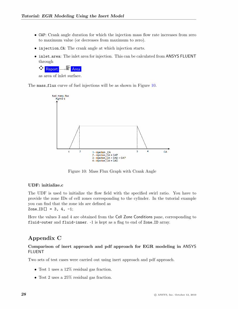
• CAP: Crank angle duration for which the injection mass flow rate increases from zeroto maximum value (or decreases from maximum to zero).

• injection CA: The crank angle at which injection starts.

• inlet area: The inlet area for injection. This can be calculated from ANSYS FLUENTthrough

Report −→ Area

as area of inlet surface.

The mass flux curve of fuel injections will be as shown in Figure 10.

Figure 10: Mass Flux Graph with Crank Angle

UDF: initialize.c

The UDF is used to initialize the flow field with the specified swirl ratio. You have toprovide the zone IDs of cell zones corresponding to the cylinder. In the tutorial exampleyou can find that the zone ids are defined asZone ID[] = 3, 4, -1;

Here the values 3 and 4 are obtained from the Cell Zone Conditions pane, corresponding tofluid-outer and fluid-inner. -1 is kept as a flag to end of Zone ID array.

Appendix C

Comparison of inert approach and pdf approach for EGR modeling in ANSYSFLUENT

Two sets of test cases were carried out using inert approach and pdf approach.

• Test 1 uses a 12% residual gas fraction.

• Test 2 uses a 25% residual gas fraction.



Test 1 : Comparison

Figure 11: Average In-Cylinder Static Pressure Curve

Figure 12: Average In-Cylinder Static Temperature Curve



Test 2 : Comparison

Figure 13: Average In-Cylinder Static Pressure Curve

Figure 14: Average In-Cylinder Static Temperature Curve

Summary

• The inert assumption showed very little impact on the solution with residual gas massfraction at 12%

• With residual gas mass fraction of 25%, the inert assumption starts to show impacton the solution.

• The tests were done with slightly lean (equivalence ratio of 0.9) condition. The inertassumption is expected to be less accurate for richer conditions and more accurate forleaner conditions.


fluent ic tut 09 inert

Documents

egr modeling

egr combustion

equilibrium of egr

egr comesin

ways of modeling egr

inert gas

modeling combustion

inert treatment