fluid dynamic investigation of the height effect of an

International Journal of Fluid Mechanics & Thermal Sciences 2015; 1(1): 1-7

Published online April 23, 2015 (http://www.sciencepublishinggroup.com/j/ijfmts)

doi: 10.11648/j.ijfmts.20150101.11

Editor-in-Chief: Zied Driss

National School of Engineers of Sfax (ENIS), Laboratory of Electro-Mechanical Systems (LASEM), University of Sfax Tunisia

Fluid Dynamic Investigation of the Height Effect of an Inclined Roof Obstacle

Slah Driss, Zied Driss, Imen Kallel Kammoun

Laboratory of Electro-Mechanic Systems (LASEM), National School of Engineers of Sfax (ENIS), Univrsity of Sfax, Sfax, Tunisia

Email address: [email protected] (S. Driss), [email protected] (Z. Driss), [email protected] (I. K. Kammoun)

To cite this article: Slah Driss, Zied Driss, Imen Kallel Kammoun. Fluid Dynamic Investigation of the Height Effect of an Inclined Roof Obstacle. International

Journal of Fluid Mechanics & Thermal Sciences. Vol. 1, No. 1, 2015, pp. 1-7. doi: 10.11648/j.ijfmts.20150101.11

Abstract: The present paper is dedicated to the numerical simulation of the height effect of an inclined roof obstacle. The

governing equations of mass and momentum in conjunction with the standard k-ε turbulence model are solved using the

computational fluid Dynamics (CFD). The numerical method used a finite volume discretization. Experiments in wind tunnel are

also developed to measure the average velocity near two inclined roof obstacles. The numerical simulations agreed reasonably

with the experimental results and the numerical model was validated.

Keywords: Fluid Dynamic, Height Effect, Inclined Roof Obstacle, Wind Tunnel

1. Introduction

Air quality within an urban street canyon is influenced by

traffic flow and its emissions, urban background

concentrations, ambient meteorological parameters, and

building geometry configurations such as roof shape, building

height, street width, etc. In this context, Nozawa [1] studied

the turbulent inflow data generated for both a smooth surface

and rough surfaces lyres. Ikhwan et al. [2] conducted in a

boundary layer wind tunnel. The velocities of the flow around

the pyramids and the pressure distribution on the pyramid

surfaces were measured using 2D laser Doppler anemometry

(LDA) and standard pressure tapping technique, respectively.

Eight different pyramids with varying base angles were

investigated. The mean and fluctuating characteristics that

distinguish pyramids field around pyramids surfaces are

described. Ahmad et al. [3] provided a comprehensive

literature on wind tunnel simulation studies in urban street

including the effects of building configurations, canyon

geometries, traffic induced turbulence and variable

approaching wind directions on flow fields and exhaust

dispersion. Melo et al. [4] developed two Gaussian

atmospheric dispersion models, AERMOD and CALPUFF.

Both incorporating the PRIME algorithm for plume rise and

building downwash, are intercompared and validated using

wind tunnel data on odour dispersion around a complex pig

farm facility comprising of two attached buildings. The results

show that concentrations predicted by AERMOD are in

general higher than those predicted by CALPUFF, especially

regarding the maximum mean concentrations observed in the

near field. Comparison of the model results with wind tunnel

data showed that both models adequately predict mean

concentrations further downwind from the facility. However,

closer to the buildings, the models may over-predict or

under-predict concentrations by a factor of two, and in certain

cases even larger, depending on the conditions. Tominaga and

Stathopoulos [5] reviewed current modeling techniques in

CFD simulation of near-field pollutant dispersion in urban

environments and discussed the findings to give insight into

future applications. Ould Said et al. [6] dedicated to the

numerical simulation of thermal convection in a two

dimensional vertical conical cylinder partially annular space.

The governing equations of mass, momentum and energy are

solved using the CFD code “FLUENT”. The results of

streamlines and the isotherms of the fluid are discussed for

different annuli with various boundary conditions and

Rayleigh numbers. Princevac et al. [7] observed and

quantitatively measured, within regular 3x3 and 5x5 arrays of

cubes, a sideways mean inflow in the lee of all succeeding

rows of buildings. When the central building in a 3x3 array is

replaced by a building of double height, due to the strong

downdraft caused by this tall building, the lateral outflow

becomes significantly more intense. Lateb et al. [8]

determined the turbulence model that best helped reproduce

2 Slah Driss, Zied Driss et al.: Fluid Dynamic Investigation of the Height Effect of an Inclined Roof Obstacle

pollutant plume dispersion. The most critical case was

considered, namely, when wind blew perpendicularly towards

the upstream tower, then placing the building in its wake.

When numerical results were compared to wind tunnel

experiments, it was found that the realizable k-ε turbulence

model yielded the best agreement with wind tunnel results for

the lowest stack height. For the highest stack height, the RNG

k-ε turbulence model provided greater concordance with

experimental results. Vizotto [9] developed a computational

model of free-form shell generation in the design of roof

structures that rely on the optimized behaviour of the

membrane theory of thin shells. For architects and engineers,

the model offers a low cost, fast, and relatively easy design

solution. Jiang et al. [10] studied three ventilation cases,

single-sided ventilation with an opening in windward wall,

single-sided ventilation with an opening in leeward wall, and

cross ventilation. In the wind tunnel, a laser Doppler

anemometry was used to provide accurate and detailed

velocity data. In LES calculations, two subgrid-scale (SS)

models, a Smagorinsky SS model and a filtered dynamic SS

model, were used. The numerical results from LES are in good

agreement with the experimental data, in particular with the

predicted airflow patterns. Fabien et al. [11] developed a

theoretical model for the calculation of driving rain by which

the infuence of wind, building geometry and rainfall on the

driving-rain intensity distributions on building envelopes can

be studied. In this model a catch ratio is introduced which

depends on raindrop diameter, reference wind speed in the

undisturbed wind flow, on building geometry and on the

position on the building envelope. By the use of computational

fluid dynamics catch ratios for several wind speeds and

geometries have been calculated. Driving-rain intensities and

its distribution on the envelope can be calculated with a

chosen raindrop spectrum. Lim et al. [12] presented a

numerical simulation of flow around a surface mounted cube

placed in a turbulent boundary layer which, although

representing a typical wind environment, to match a series of

wind tunnel observations. The simulations were carried out at

a Reynolds number, based on the velocity at the cube height,

of 20,000. The results presented include detailed comparison

between measurements and LES computations of both the

inflow boundary layer and the flow field around the cube

including mean and fluctuating surface pressures. Ntinas et al.

[13] predicted the airflow around buildings. A time-dependent

simulation model has been applied for the prediction of the

turbulent airflow around obstacles with arched and pitched

roof geometry, under wind tunnel conditions. To verify the

reliability of the model, an experiment was conducted inside a

wind tunnel and the air velocity and turbulent kinetic energy

profiles were measured around two small-scale obstacles with

an arched-type and a pitched-type roof. Luo et al. [15] studied

models of cuboid obstacles to characterize the

three-dimensional responses of airflow behind obstacles with

different shape ratios to variations in the incident flow in a

wind-tunnel simulation. Wind velocity was measured using

particle image velocimetry (PIV). The flow patterns behind

cuboid obstacles were complicated by changes in the

incidence angle of the approaching flow and in the obstacle's

shape ratio.

According to these anterior studies, it’s clear that the study

of the aerodynamic around the obstacle is very interesting.

Indeed, the literature review confirms that there is paucity on

the inclined roof obstacle study. For thus, we are interested on

the study of the height effect of an inclined roof obstacle.

2. Numerical Model

2.1. Geometrical Parameters

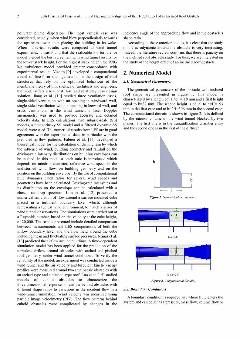
The geometrical parameters of the obstacle with inclined

roof shape are presented in figure 1. This model is

characterized by a length equal to l=118 mm and a first height

equal to b=82 mm. The second height is equal to h=H=153

mm in the first case and to h=2H=306 mm in the second case.

The computational domain is shown in figure 2. It is defined

by the interior volume of the wind tunnel blocked by two

planes. The first one is in the tranquillization chamber entry

and the second one is in the exit of the diffuser.

Figure 1. Geometrical arrangement.

(a) h=H

(b) h=2 H

Figure 2. Computational domain.

2.2. Boundary Conditions

A boundary condition is required any where fluid enters the

system and can be set as a pressure, mass flow, volume flow or

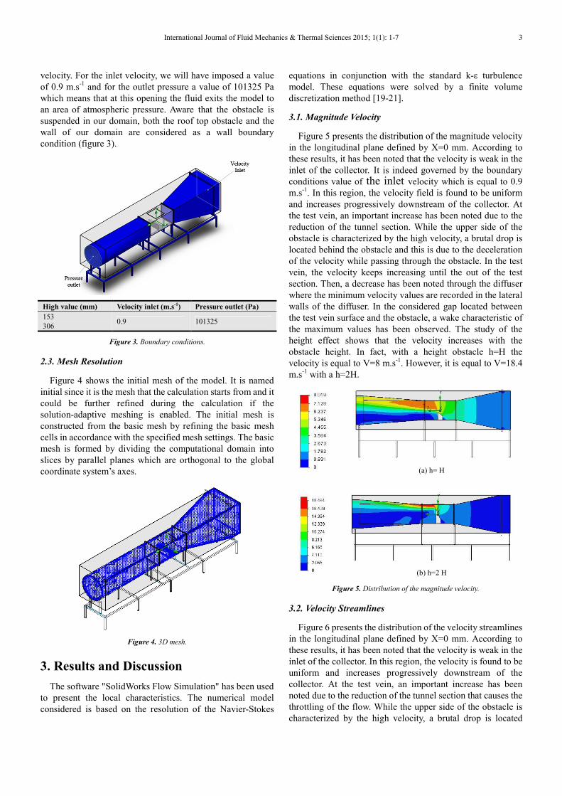
International Journal of Fluid Mechanics & Thermal Sciences 2015; 1(1): 1-7 3

velocity. For the inlet velocity, we will have imposed a value

of 0.9 m.s-1

and for the outlet pressure a value of 101325 Pa

which means that at this opening the fluid exits the model to

an area of atmospheric pressure. Aware that the obstacle is

suspended in our domain, both the roof top obstacle and the

wall of our domain are considered as a wall boundary

condition (figure 3).

High value (mm) Velocity inlet (m.s-1) Pressure outlet (Pa)

153 0.9 101325

306

Figure 3. Boundary conditions.

2.3. Mesh Resolution

Figure 4 shows the initial mesh of the model. It is named

initial since it is the mesh that the calculation starts from and it

could be further refined during the calculation if the

solution-adaptive meshing is enabled. The initial mesh is

constructed from the basic mesh by refining the basic mesh

cells in accordance with the specified mesh settings. The basic

mesh is formed by dividing the computational domain into

slices by parallel planes which are orthogonal to the global

coordinate system’s axes.

Figure 4. 3D mesh.

3. Results and Discussion

The software "SolidWorks Flow Simulation" has been used

to present the local characteristics. The numerical model

considered is based on the resolution of the Navier-Stokes

equations in conjunction with the standard k-ε turbulence

model. These equations were solved by a finite volume

discretization method [19-21].

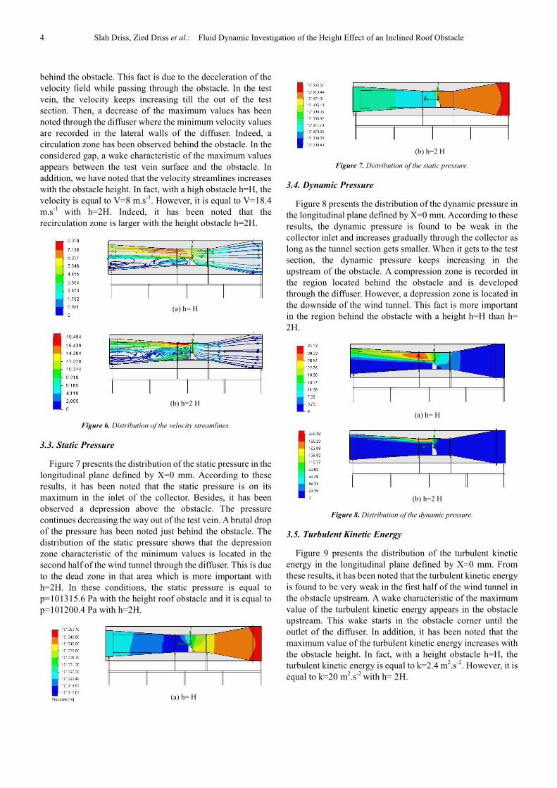
3.1. Magnitude Velocity

Figure 5 presents the distribution of the magnitude velocity

in the longitudinal plane defined by X=0 mm. According to

these results, it has been noted that the velocity is weak in the

inlet of the collector. It is indeed governed by the boundary

conditions value of the inlet velocity which is equal to 0.9

m.s-1

. In this region, the velocity field is found to be uniform

and increases progressively downstream of the collector. At

the test vein, an important increase has been noted due to the

reduction of the tunnel section. While the upper side of the

obstacle is characterized by the high velocity, a brutal drop is

located behind the obstacle and this is due to the deceleration

of the velocity while passing through the obstacle. In the test

vein, the velocity keeps increasing until the out of the test

section. Then, a decrease has been noted through the diffuser

where the minimum velocity values are recorded in the lateral

walls of the diffuser. In the considered gap located between

the test vein surface and the obstacle, a wake characteristic of

the maximum values has been observed. The study of the

height effect shows that the velocity increases with the

obstacle height. In fact, with a height obstacle h=H the

velocity is equal to V=8 m.s-1

. However, it is equal to V=18.4

m.s-1

with a h=2H.

(a) h= H

(b) h=2 H

Figure 5. Distribution of the magnitude velocity.

3.2. Velocity Streamlines

Figure 6 presents the distribution of the velocity streamlines


these results, it has been noted that the velocity is weak in the

inlet of the collector. In this region, the velocity is found to be

uniform and increases progressively downstream of the

collector. At the test vein, an important increase has been

noted due to the reduction of the tunnel section that causes the

throttling of the flow. While the upper side of the obstacle is

characterized by the high velocity, a brutal drop is located


behind the obstacle. This fact is due to the deceleration of the

velocity field while passing through the obstacle. In the test

vein, the velocity keeps increasing till the out of the test

section. Then, a decrease of the maximum values has been

noted through the diffuser where the minimum velocity values

are recorded in the lateral walls of the diffuser. Indeed, a

circulation zone has been observed behind the obstacle. In the

considered gap, a wake characteristic of the maximum values

appears between the test vein surface and the obstacle. In

addition, we have noted that the velocity streamlines increases

with the obstacle height. In fact, with a high obstacle h=H, the

velocity is equal to V=8 m.s-1

. However, it is equal to V=18.4

m.s-1

with h=2H. Indeed, it has been noted that the

recirculation zone is larger with the height obstacle h=2H.

(a) h= H

(b) h=2 H

Figure 6. Distribution of the velocity streamlines.

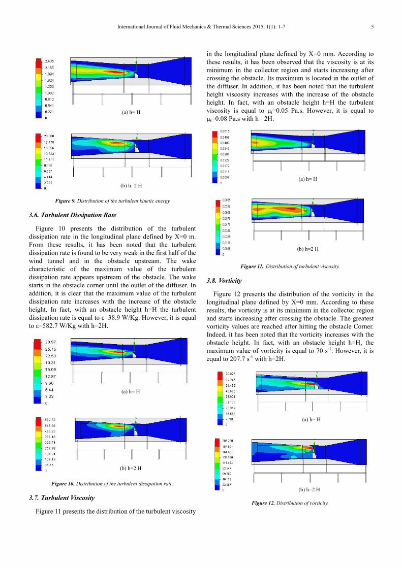
3.3. Static Pressure

Figure 7 presents the distribution of the static pressure in the

longitudinal plane defined by X=0 mm. According to these

results, it has been noted that the static pressure is on its

maximum in the inlet of the collector. Besides, it has been

observed a depression above the obstacle. The pressure

continues decreasing the way out of the test vein. A brutal drop

of the pressure has been noted just behind the obstacle. The

distribution of the static pressure shows that the depression

zone characteristic of the minimum values is located in the

second half of the wind tunnel through the diffuser. This is due

to the dead zone in that area which is more important with

h=2H. In these conditions, the static pressure is equal to

p=101315.6 Pa with the height roof obstacle and it is equal to

p=101200.4 Pa with h=2H.

(a) h= H

(b) h=2 H

Figure 7. Distribution of the static pressure.

3.4. Dynamic Pressure

Figure 8 presents the distribution of the dynamic pressure in

the longitudinal plane defined by X=0 mm. According to these

results, the dynamic pressure is found to be weak in the

collector inlet and increases gradually through the collector as

long as the tunnel section gets smaller. When it gets to the test

section, the dynamic pressure keeps increasing in the

upstream of the obstacle. A compression zone is recorded in

the region located behind the obstacle and is developed

through the diffuser. However, a depression zone is located in

the downside of the wind tunnel. This fact is more important

in the region behind the obstacle with a height h=H than h=

2H.

(a) h= H

(b) h=2 H

Figure 8. Distribution of the dynamic pressure.

3.5. Turbulent Kinetic Energy

Figure 9 presents the distribution of the turbulent kinetic

energy in the longitudinal plane defined by X=0 mm. From

these results, it has been noted that the turbulent kinetic energy

is found to be very weak in the first half of the wind tunnel in

the obstacle upstream. A wake characteristic of the maximum

value of the turbulent kinetic energy appears in the obstacle

upstream. This wake starts in the obstacle corner until the

outlet of the diffuser. In addition, it has been noted that the

maximum value of the turbulent kinetic energy increases with

the obstacle height. In fact, with a height obstacle h=H, the

turbulent kinetic energy is equal to k=2.4 m2.s

-2. However, it is

equal to k=20 m2.s

-2 with h= 2H.


(a) h= H

(b) h=2 H

Figure 9. Distribution of the turbulent kinetic energy

3.6. Turbulent Dissipation Rate

Figure 10 presents the distribution of the turbulent

dissipation rate in the longitudinal plane defined by X=0 m.

From these results, it has been noted that the turbulent

dissipation rate is found to be very weak in the first half of the

wind tunnel and in the obstacle upstream. The wake

characteristic of the maximum value of the turbulent

dissipation rate appears upstream of the obstacle. The wake

starts in the obstacle corner until the outlet of the diffuser. In

addition, it is clear that the maximum value of the turbulent

dissipation rate increases with the increase of the obstacle

height. In fact, with an obstacle height h=H the turbulent

dissipation rate is equal to ε=38.9 W/Kg. However, it is equal

to ε=582.7 W/Kg with h=2H.

(a) h= H

(b) h=2 H

Figure 10. Distribution of the turbulent dissipation rate.

3.7. Turbulent Viscosity

Figure 11 presents the distribution of the turbulent viscosity


these results, it has been observed that the viscosity is at its

minimum in the collector region and starts increasing after

crossing the obstacle. Its maximum is located in the outlet of

the diffuser. In addition, it has been noted that the turbulent

height viscosity increases with the increase of the obstacle

height. In fact, with an obstacle height h=H the turbulent

viscosity is equal to µt=0.05 Pa.s. However, it is equal to

µt=0.08 Pa.s with h= 2H.

(a) h= H

(b) h=2 H

Figure 11. Distribution of turbulent viscosity.

3.8. Vorticity

Figure 12 presents the distribution of the vorticity in the

longitudinal plane defined by X=0 mm. According to these

results, the vorticity is at its minimum in the collector region

and starts increasing after crossing the obstacle. The greatest

vorticity values are reached after hitting the obstacle Corner.

Indeed, it has been noted that the vorticity increases with the

obstacle height. In fact, with an obstacle height h=H, the

maximum value of vorticity is equal to 70 s-1

. However, it is

equal to 207.7 s-1

with h=2H.

(a) h= H

(b) h=2 H

Figure 12. Distribution of vorticity.


4. Comparison with Experimental

Results

The wind tunnel results are used to validate the CFD model.

The experiment is carried out in the atmospheric boundary

layer wind tunnel at the National school of Engineering of

Sfax, Tunisia. The simulated data are interpolated at the same

grid points as in the wind tunnel experiment (figure 13). As the

configuration is replicated from the wind tunnel experiment,

the CFD model tested using the mathematical model is

validated against the data obtained from the wind tunnel

experiments. The velocity profiles are chosen for points

situated in the test section. The considered planes are defined

by Z=0 mm, Z=150 mm and Z= -150 mm. For each transverse

planes, values are taken along the directions defined by X=0

mm. The results for each plane are shown in figure 14.

According to these profiles, it has been noted that the velocity

value is very weak near the obstacle. Outside, the velocity has

a maximum value. The comparison between the numerical

and experimental results leads us to the conclusion that despite

some unconformities, the values are comparable. The

numerical model seems to be able to predict the aerodynamic

characteristics of the air flow around the obstacle.

Figure 13. Wind tunnel.

(a) Z=0 mm and X=0 mm

(b) Z=150 mm and X=0 mm

(c) z=-150 mm and x=0 mm

Figure 14. Velocity profils.

5. Conclusion

In this work, we have developed a numerical simulation to

study the height effect of an inclined roof obstacle on the

aerodynamic characteristics. Numerical results, such as

velocity fields, pressure and turbulent characteristics are

presented in the wind tunnel. According to the numerical

results, it has been noted that the roof obstacle shape has a

direct effect on the local characteristics. The study of the

height effect shows that the velocity increases with the

obstacle height and the recirculation zones become larger.

Also, the maximum values of the turbulent characteristics

increase with the obstacle height. Use of this knowledge will

assist the design of packaged installations of the wind rotors

in the buildings. In the future, we propose to apply this study

on the building design.

References

[1] Nozawa, K., Tamura, I.N., 2002, Large eddy simulation of the flow around a low-rise building immersed in a rough-wall turbulent boundary layer , Journal of Wind Engineering and Industrial Aerodynamics, 90, 1151-1162.

[2] Ikhwan, M., Ruck, B., 2006, Flow and pressure field characteristics around pyramidal buildings, Journal of Wind Engineering and Industrial Aerodynamics, 94 745-765.


[3] Ahmad, K., Khare, M., Chaudhry, K.K., 2005, Wind tunnel simulation studies on dispersion at urban street canyons and intersections-a review, Journal of Wind Engineering and Industrial Aerodynamics, 90, 697-717.

[4] De Melo, A. M. V., Santos, J. M., Mavrroidis, I. , Reis Junior, N. C., 2012, Modelling of odour dispersion around a pig farm building complex using AERMOD and CALPUFF. Comparison with wind tunnel results, Building and Environment, 56, 8-20.

[5] Tominaga, Y., Stathopoulos, T., 2013, CFD simulation of near-field pollutant dispersion in the urban environment: A review of current modeling techniques, Atmospheric Environment, 79, 716-730.

[6] Ould said, B., Retiel, N., Bouguerra, E.H., 2014, Numerical Simulation of Natural Convection in a Vertical Conical Cylinder Partially Annular Space, American Journal of Energy Research, 2(2), 24-29.

[7] Princevac, M. Baik, J. Li, X., Pan, H., Park, S. , 2010, Lateral channeling within rectangular arrays of cubical obstacles, Journal of Wind Engineering and Industrial Aerodynamics, 98, 377-385.

[8] Lateb, M., Masson, C., Stathopoulos, T., Bédard, C., 2013, Comparison of various type of k- ε models for pollutant emissions around a two-building configuration, Journal of Wind Engineering and Indusrial Aerodynamics, 115, 9-21.

[9] Vizotto, I., Computational generation of free-form shells in architectural design and civil engineering, Automation in construction, 19, 1087-1105

[10] Jiang, Y., Alexander, D., Jenkins, H., Arthur, R., Chen, Q., 2003, Natural ventilation in buildings: measurement in a wind tunnel and numerical simulation with large-eddy simulation, Journal of Wind Engineering and Industrial Aerodynamics, 91, 331-353.

[11] Fabien, J.R., Martin, H., Jacob, W., Computer Simulation Of Driving Rain On Building Envelopes, 2nd European and African Conference on Wind Engineering, Genova, 22-26 June 1997.

[12] Lim, H.C., Thomas, T.G., Castro, I.P., 2009, Flow around a cube in a turbulent boundary layer: LES and experiment, Journal of Wind Engineering and Industrial Aerodynamics, 97, 96-109.

[13] Ntinas, G.K., Zhangb, G., Fragos, V.P., Bochtis, D.D., Nikita-Martzopoulou, C., 2014, Airflow patterns around obstacles with arched and pitched roofs: Wind tunnel measurements and direct simulation, European Journal of Mechanics B/Fluids, 43, 216-229.

[14] Luo, W., Dong, Z., Qian, G., Lu, J., 2012, Wind tunnel simulation of the three-dimensional airflow patterns behind cuboid obstacles at different angles of wind incidence and their significance for theformation of sand shadows, Geomorphology, 139-140, 258-270.

[15] Rafailidis, S., Schatzmann, M., 1995, Concentration Measurements with Different Roof Patterns in Street Canyon with Aspect Ratios B/H¼1/2 and B/H¼1, Universität Hamburg, Meterologisches Institute.

[16] Driss, Z., Bouzgarrou, G., Chtourou, W., Kchaou, H., Abid, M.S., 2010, Computational studies of the pitched blade turbines design effect on the stirred tank flow characteristics, European Journal of Mechanics B/Fluids, 29, 236-245.

[17] Ammar, M., Chtourou, W., Driss, Z., Abid, M.S., 2011, Numerical investigation of turbulent flow generated in baffled stirred vessels equipped with three different turbines in one and two-stage system, Energy, 36, 5081-5093.

[18] Driss, Z., Abid, M.S., 2012, Use of the Navier-Stokes Equations to Study of the Flow Generated by Turbines Impellers. Navier-Stokes Equations: Properties, Description and Applications, 3, 51-138.

[19] Driss, S, Driss, Z, Kallel Kammoun, I, 2014, Study of the Reynolds Number Effect on the Aerodynamic Structure around an Obstacle with Inclined Roof, Sustainable Energy, 2( 4), 126-133.

[20] Driss, Z., Ammar, M., Chtourou, W., Abid, M.S., 2011, CFD Modelling of Stirred Tanks. Engineering Applications of Computational Fluid Dynamics, 5, 145-258.

fluid dynamic investigation of the height effect of an

Documents