1

FLUID FLOW VISUALIZATIONFrits H. Post, Theo van Walsum

Delft University of Technology, The Netherlands*

Published in: Focus on Scientific Visualization, H. Hagen, H. Müller, G.M. Nielson (eds.),Springer Verlag, Berlin, 1993, pp. 1-40 (ISBN 3-540-54940-4)

Abstract

This paper presents an overview of techniques for visualization of fluid flow data. As a startingpoint, a brief introduction to experimental flow visualization is given. The rest of the paperconcentrates on computer graphics flow visualization. A pipeline model of the flow visualizationprocess is used as a basis for presentation. Conceptually, this process centres around visualizationmapping, or the translation of physical flow parameters to visual representations. Starting from aset of standard mappings partly based on equivalents from experimental visualization, a number ofdata preparation techniques is described, to prepare the flow data for visualization. Next, a numberof perceptual effects and rendering techniques are described, and some problems in visualpresentation are discussed. The paper ends with some concluding remarks and suggestions forfuture development.

1 Introduction

For centuries, fluid flow researchers have been studying fluid flows in various ways, and todayfluid flow is still an important field of research. The areas in which fluid flow plays a role arenumerous. Gaseous flows are studied for the development of cars, aircraft and spacecrafts, andalso for the design of machines such as turbines and combustion engines. Liquid flow research isnecessary for naval applications, such as ship design, and is widely used in civil engineeringprojects such as harbour design and coastal protection. In chemistry, knowledge of fluid flow inreactor tanks is important; in medicine, the flow in blood vessels is studied. Numerous otherexamples could be mentioned. In all kinds of fluid flow research, visualization is an key issue.

1.1 Purposes and Problems of Flow Visualization

Flow visualization probably exists as long as fluid flow research itself. Until recently,experimental flow visualization, as described in section 2, has been the main visualization aid influid flow research. Experimental flow visualization techniques are applied for several reasons:

• to get an impression of fluid flow around a scale model of a real object, without anycalculations;

• as a source of inspiration for the development of new and better theories of fluid flow;• to verify a new theory or model.

Though used extensively, these methods suffer from some problems. A fluid flow is oftenaffected by the experimental technique, and not all fluid flow phenomena or relevant parameterscan be visualized with experimental techniques. Also, the construction of small scale physicalmodels, and experimental equipment such as wind tunnels are expensive, and experiments are timeconsuming.

* Department of Technical Informatics, Zuidplantsoen 4, 2628 BZ Delft, The Netherlands. Email:frits.post@cs.tudelft.nl

2

Recently a new type of visualization has emerged: computer-aided visualization. The increaseof computational power has led to an increasing use of computers for numerical simulations. In thearea of fluid dynamics, computers are extensively used to calculate velocity fields and other flowquantities, using numerical techniques to solve the governing Navier-Stokes equations. This hasled to the emergence of Computational Fluid Dynamics (CFD) as a new field of research andpractice.

To analyse the results of the complex calculations, computer visualization techniques arenecessary. Humans are capable of comprehending much more information when it is presentedvisually, rather than numerically. By using the computer not only for calculating the numericaldata, but also for visualizing these data in an understandable way, the benefits of the increasingcomputational power are much greater.

The visualization of fluid flow simulation data may have several different purposes. Onepurpose is the verification of theoretical models in fundamental research. When a flowphenomenon is described by a model, this flow model should be compared with the ‘real’ fluidflow. The accuracy of the model can be verified by calculation and visualization of a flow with themodel, and comparison of the results with experimental results. If the numerical results and theexperimental flow are visualized in the same way, a qualitative verification by visual inspection canbe very effective. Research in numerical methods for solving the flow equations can be supportedby visualizing the solutions found, but also by visualization of intermediate results during theiterative solution process.

Another purpose of fluid flow visualization is the analysis and evaluation of a design. For thedesign of a car, an aircraft, a harbour, or any other object that is functionally related with fluidflow, calculation and visualization of the fluid flow phenomena can be an powerful tool in designoptimization and evaluation. In this type of applied research, communication of flow analysisresults to others, including non-specialists, is important in the decision making process.

In practice, often both experimental and computer-aided visualization will be applied. Fluidflow visualization using computer graphics will be inspired by experimental visualization.Following the development of 3D flow solution techniques, there is especially an urgent need forvisualization of 3D flow patterns. This presents many interesting but still unsolved problems tocomputer graphics research. Flow data are different in many respects from the objects and surfacestraditionally displayed by 3D computer graphics. New techniques are emerging for generatinginformative images of flow patterns; also, techniques are being developed to transform the flowvisualization problem to display of traditional graphics primitives.

1.2 Overview

The main purpose of this paper is to give an introduction to fluid flow visualization with computergraphics. It was primarily written for the computer graphics students interested in scientificvisualization, and therefore some knowledge of basic computer graphics concepts and techniquesis assumed. No knowledge of fluid dynamics is assumed; readers interested in the principles offluid dynamics theory are referred to text books on fluid dynamics (such as Batchelor, ‘67). Thispaper will also be useful for CFD specialists who want to know more about techniques available tovisualize their data. An attempt has been made to provide a connection of the visualization processwith the CFD simulation process. For basic graphics techniques they should refer to text books oncomputer graphics (such as Foley et al., ‘90).

Before we turn to computer-aided visualization flow techniques, we will briefly discuss someconcepts and methods from experimental flow visualization (section 2). In section 3, a pipelinemodel of the flow visualization process is introduced, and two important stages of the pipeline are

3

described: visualization mapping and data preparation and analysis techniques. Section 4 describescomputer graphics presentation techniques, based on a set of standard forms of flow visualizationdescribed in section 3. Some additional topics in rendering and animation will also be discussed.Finally, in section 5, some conclusions are drawn and directions for research are indicated.

2 Experimental Flow Visualization

Experimental flow visualization has a long history, and today a wide variety of techniques tovisualize fluid flows is known. Merzkirch (‘87) and Yang (‘89) give an overview of thefundamental techniques for flow visualization and describe a number of applications of thesetechniques. Van Dyke (‘82) shows many excellent pictures of experimental fluid flowexperiments.

Following Merzkirch (‘87), three basic types of visualization can be distinguished: addingforeign material (2.1), optical techniques (2.2), and adding heat and energy (2.3).

2.1 Addition of Foreign Material

Time lines, streak lines and path lines play an important role in experimental fluid flowvisualization techniques:

• Time lines are lines that, once released in the fluid, are moved and transformed by the fluidflow. The motion and formation of the line, which is often released perpendicular to theflow, shows the fluid flow. In practice, time lines often consist of a row of small particles,such as hydrogen bubbles.

• A streak line arises when dye is injected in the flow from a fixed position. Injecting the dyefor a period of time gives a line of dye in the fluid, from which the fluid flow can be seen.

• A path line is the path of a particle in the fluid. Imagine a light-emitting particle in the flow.A path line is obtained when a photographic plate is exposed for several seconds.

We will see in section 3 and 4 that time lines, streak lines, and path lines also play animportant role in computer graphics flow visualization. In steady flows, streak lines and path linescoincide. In that case, streak lines and path lines are identical to stream lines, lines that areeverywhere tangent to the velocity field.

Time lines, streak lines or path lines can be visualized by injecting foreign material in the fluid,which in general is transparent. As already mentioned, streak lines can be created by injecting dyein the (liquid) fluid. An example of an application of flow visualization using dye is shown infigure 2.1. In case of a gas flow, smoke can be injected in the fluid. Though conceptually simple,these techniques require very careful application. The injection itself can disturb the flow. Thedensity and temperature of the injected material, if not equal to that of the flow at the injection spot,can also influence the flow field.

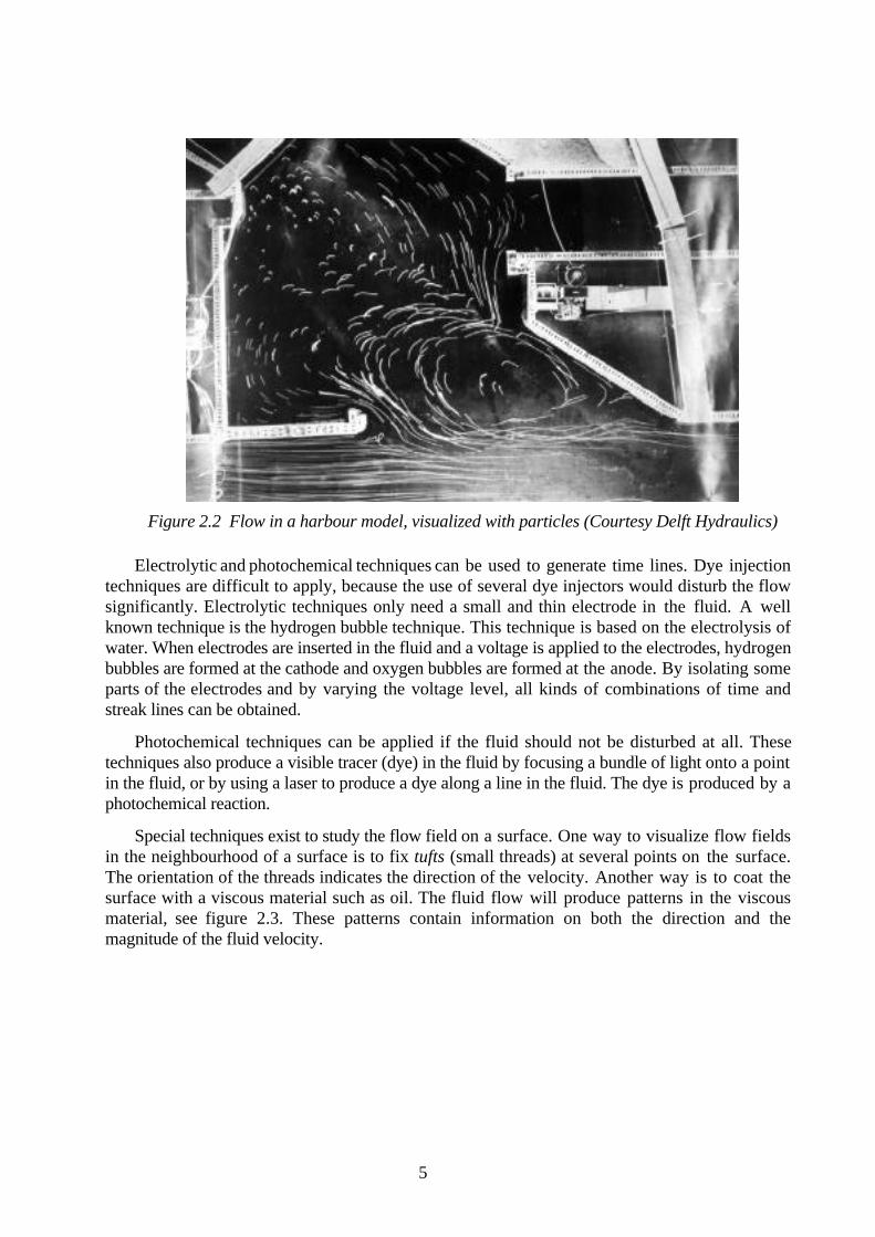
Path lines are generated by adding small particles to the fluid. An example of suitable particlesfor liquid fluid is magnesium powder; in gaseous fluids, oil droplets can be used. The velocity canbe measured by photographing the motion of the particles with a known exposure time (see figure2.2).

4

Figure 2.1 Visualization with dye to study water flow in a river model(Courtesy Delft Hydraulics)

5

Figure 2.2 Flow in a harbour model, visualized with particles (Courtesy Delft Hydraulics)

Electrolytic and photochemical techniques can be used to generate time lines. Dye injectiontechniques are difficult to apply, because the use of several dye injectors would disturb the flowsignificantly. Electrolytic techniques only need a small and thin electrode in the fluid. A wellknown technique is the hydrogen bubble technique. This technique is based on the electrolysis ofwater. When electrodes are inserted in the fluid and a voltage is applied to the electrodes, hydrogenbubbles are formed at the cathode and oxygen bubbles are formed at the anode. By isolating someparts of the electrodes and by varying the voltage level, all kinds of combinations of time andstreak lines can be obtained.

Photochemical techniques can be applied if the fluid should not be disturbed at all. Thesetechniques also produce a visible tracer (dye) in the fluid by focusing a bundle of light onto a pointin the fluid, or by using a laser to produce a dye along a line in the fluid. The dye is produced by aphotochemical reaction.

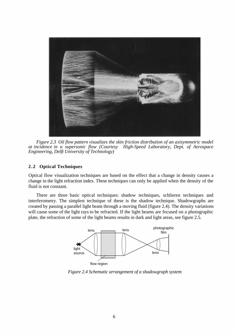
Special techniques exist to study the flow field on a surface. One way to visualize flow fieldsin the neighbourhood of a surface is to fix tufts (small threads) at several points on the surface.The orientation of the threads indicates the direction of the velocity. Another way is to coat thesurface with a viscous material such as oil. The fluid flow will produce patterns in the viscousmaterial, see figure 2.3. These patterns contain information on both the direction and themagnitude of the fluid velocity.

6

Figure 2.3 Oil flow pattern visualizes the skin friction distribution of an axisymmetric modelat incidence in a supersonic flow (Courtesy High-Speed Laboratory, Dept. of AerospaceEngineering, Delft University of Technology)

2.2 Optical Techniques

Optical flow visualization techniques are based on the effect that a change in density causes achange in the light refraction index. These techniques can only be applied when the density of thefluid is not constant.

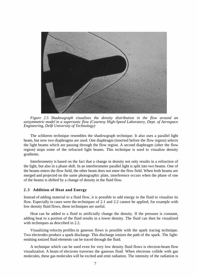
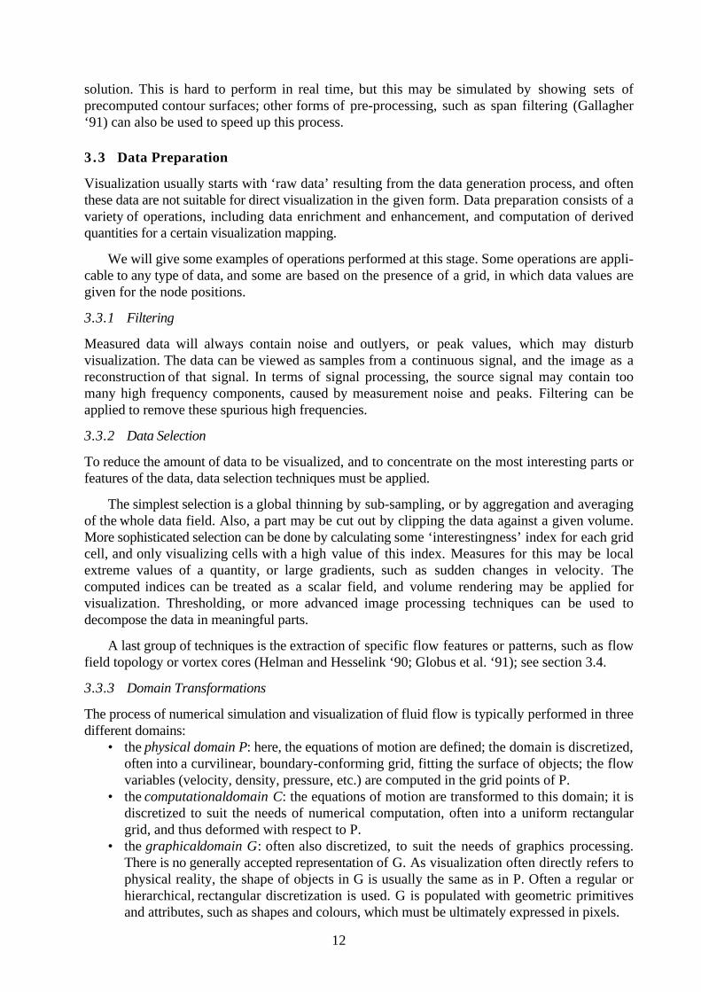
There are three basic optical techniques: shadow techniques, schlieren techniques andinterferometry. The simplest technique of these is the shadow technique. Shadowgraphs arecreated by passing a parallel light beam through a moving fluid (figure 2.4). The density variationswill cause some of the light rays to be refracted. If the light beams are focused on a photographicplate, the refraction of some of the light beams results in dark and light areas, see figure 2.5.

light source

photographicfilm

flow region

lens lens

lens

Figure 2.4 Schematic arrangement of a shadowgraph system

7

Figure 2.5 Shadowgraph visualizes the density distribution in the flow around anaxisymmetric model in a supersonic flow (Courtesy High-Speed Laboratory, Dept. of AerospaceEngineering, Delft University of Technology)

The schlieren technique resembles the shadowgraph technique. It also uses a parallel lightbeam, but now two diaphragms are used. One diaphragm (inserted before the flow region) selectsthe light beams which are passing through the flow region. A second diaphragm (after the flowregion) stops some of the refracted light beams. This technique is used to visualize densitygradients.

Interferometry is based on the fact that a change in density not only results in a refraction ofthe light, but also in a phase shift. In an interferometer parallel light is split into two beams. One ofthe beams enters the flow field, the other beam does not enter the flow field. When both beams aremerged and projected on the same photographic plate, interference occurs when the phase of oneof the beams is shifted by a change of density in the fluid flow.

2.3 Addition of Heat and Energy

Instead of adding material to a fluid flow, it is possible to add energy to the fluid to visualize itsflow. Especially in cases were the techniques of 2.1 and 2.2 cannot be applied, for example withlow density fluid flows, these techniques are useful.

Heat can be added to a fluid to artificially change the density. If the pressure is constant,adding heat to a portion of the fluid results in a lower density. The fluid can then be visualizedwith techniques as described in 2.2.

Visualizing velocity profiles in gaseous flows is possible with the spark tracing technique.Two electrodes produce a spark discharge. This discharge ionizes the path of the spark. The light-emitting ionized fluid elements can be traced through the fluid.

A technique which can be used even for very low density fluid flows is electron-beam flowvisualization. A beam of electrons traverses the gaseous fluid. When electrons collide with gasmolecules, these gas molecules will be excited and emit radiation. The intensity of the radiation is

8

approximately proportional with the density of the fluid. By moving the electron beam, the entireflow area can be scanned.

3 Computer Graphics Flow Visualization

Experimental flow visualization is a starting point for flow visualization using computer graphics.The process of computer visualization is described in general, and applied to CFD (3.1). The heartof the process is the translation of physical to visual variables. Fluid mechanics theory and practicehelp to identify a set of ‘standard’ forms of visualization (3.2). To prepare the flow data to be castin visual form, several types of operations may have to be performed on the data (3.3). A specialtype of operation, analysis of the topology of a fluid flow data set, is described separately (3.4).

3.1 The Flow Visualization Process

Scientific visualization with computer-generated images can be generally conceived as a three-stagepipeline process (Haber and McNabb ‘90). We will use an extended version of this process modelhere (see figure 3.1), and discuss its application to flow data visualization.

DATA GENERATION

VISUALIZATION MAPPING(3.2)

DATA ENRICHMENT& ENHANCEMENT (3.3)

RENDERING (4)

DISPLAY (4.3.1)

Figure 3.1 A pipeline model of the visualization process

• Data generation: production of numerical data by measurement or numerical simulations.Flow data can be based on flow measurements, or can be derived from analysis of imagesobtained with experimental visualization techniques as described in section 2, using imageprocessing (Yang ‘89). Numerical flow simulations often produce velocity fields,sometimes combined with scalar data such as pressure, temperature, or density. In the restof this paper, we will be mainly concerned with data generated by CFD simulations.

• Data enrichment and enhancement: modification or selection of the data, to reduce theamount or improve the information content of the data. Examples are domain transforma-tions, sectioning, thinning, interpolation, sampling, and noise filtering. We will discusssome of these operations in 3.3.

9

• Visualization mapping: translation of the physical data to suitable visual primitives andattributes. This is the central part of the process; the conceptual mapping involves the‘design’ of a visualization: to determine what we want to see, and how to visualize it.Abstract physical quantities are cast into a visual domain of shapes, light, colour, and otheroptical properties. Some ‘standard’ conceptual visualization mappings of flow data will bediscussed in 3.2.The actual mapping is carried out by computing derived quantities from the data suitable fordirect visualization. For flow visualization, an example of this is the computation of particlepaths from a velocity field. As this type of operations is closely related to the operations ofthe enrichment and enhancement stage, we will discuss these together in 3.3 under theheading Data Preparation.

• Rendering: transformation of the mapped data into displayable images. Typical operationshere are viewing transformations, lighting calculations, hidden surface removal, scanconversion, and filtering (anti-aliasing and motion blur). Rendering techniques for flowvisualization will be discussed in section 4.

• Display: showing the rendered images on a screen. A display can be direct output from therendering process, or be simply achieved by loading a pixel file into a frame buffer; it mayalso involve other operations such as image file format translation, data (de)compression,and colour map manipulations. For animation, a series of precomputed rendered imagesmay be loaded into main memory of a workstation, and displayed using a simple playbackprogram.

3.2 Flow Visualization Mappings

The style of visualization using numerically generated data is suggested by the formalismunderlying the numerical simulations. The two different analytical formulations of flow: Eulerianand Lagrangian, can be used to distinguish two classes of visualization styles:

• Eulerian: physical quantities are specified in fixed locations in a 3D field. Visualizationtends to produce static images of a whole study area. A typical Eulerian visualization is anarrow plot, showing flow direction arrows at all grid points.

• Lagrangian: physical quantities are linked to small particles moving with the flow throughan area, and are given as a function of starting position and time. Visualization often leadsto dynamic images (animations) of moving particles, showing only local information in theareas where particles move.

Other styles may be called indirect visualization of flow fields. A velocity field can be charac-terized by deriving certain scalar quantities, which can be visualized using volume renderingtechniques (see 4.2.6). Examples are the magnitude of velocity or vorticity, or helicity (Buning‘89). Also, instead of individual particles, concentration of particles per volume unit can becomputed, and visualized as a scalar concentration field (Hin et al. ‘90). A second type of indirectvisualization shows the effect of the flow on the geometry of certain objects, eg. deformation ofspheres (Geiben and Rumpf ‘91).

There is a number of visual representations, that can be conceived as ‘standard’ visualizationmappings in the sense of the process model described in 3.1, some of which are directly based onexperimental flow visualization: velocity arrows, stream lines, stream surfaces (ribbons), streaklines, path lines, time lines (surfaces), and contours. They can be visualized using obvious graphi-cal primitives such as points, lines, and surfaces. In section 4, we will also discuss some moreadvanced presentation techniques

Arrows are icons for vectors, and the most obvious way to visualize a velocity field withcomputer graphics is an arrow plot. Usually, arrows are tied to grid points, and indicate both

10

direction and speed at these points. In this way, a complete view of a vector field can be given; thisis a clear example of an Eulerian style visualization. Used in this way, arrows can give reasonableresults in 2D, but there are numerous problems in the 3D case. We will discuss some of theseproblems in 4.2. A special type of arrow is the stream vector, where the tail of the arrow follows astream line.

Stream lines, streak lines, path lines (or particle traces), and time lines are directly derivedfrom experimental visualization (see 2.1). They can be generated and rendered as 2D or 3D curves(see figures 3.2, 3.3, 3.4). In 3.3, some techniques used for computation of these curves will bediscussed; we will return to rendering in 4.2 and 4.3.

In 2D, stream lines characterize a general directional flow pattern very well (figure 3.2). Also,they give an indirect cue to velocity magnitude, because the distance between stream lines isinversely proportional to velocity.

Figure 3.2 Stream lines in 2D (Bertrand and Tanguy ‘88)

In 3D, stream lines can also be used, but additional depth cues are needed to locate the curvesin space. One possibility is to generate a stream surface, interpolating a set of adjacent stream lines(Hultquist ‘90). A surface interpolating only two adjacent stream lines is called a stream ribbon(Buning ‘89, Hultquist '90).

Streak lines and path lines (see figure 3.3) can be visualized as static curves, and this can beinterpreted either as a time interval in a steady flow, or as a single instant in an unsteady flow.Animation can show the curves dynamically as they change over time. Particles can also bevisualized as moving dots or objects, or as a moving texture (Van Wijk ‘90b, ‘91; see 4.2.4 and4.3.5).

11

Figure 3.3 Particle traces (Strid et al. ‘89)

Time lines drawn for a series of instants clearly show the distribution of velocity (figure 3.4).When a 2D array of particles is released at one instant in a 3D flow field, they can define a timesurface at each instant.

Figure 3.4 Time lines

Contours are curves (in 2D) or surfaces (in 3D) where a given scalar physical variable has aconstant value. Contours, also called iso-curves and iso-surfaces, do not have counterparts inexperimental visualization. Their applicability is limited to scalar data, such as pressure,temperature, or velocity magnitude, or scalar quantities derived from a vector field. An example ofthe latter is the display of pressure contours on the surface of an airplane fuselage (see figure 3.5).

Figure 3.5 Pressure contours on a surface

In 3D, contour surfaces have the advantage of visualization with a full range of visual depthcues, but a problem is the display of multiple contours in one picture. Dynamic probing of a scalarfield by interactively varying the contour value, and showing a changing contour surface is a good

12

solution. This is hard to perform in real time, but this may be simulated by showing sets ofprecomputed contour surfaces; other forms of pre-processing, such as span filtering (Gallagher‘91) can also be used to speed up this process.

3.3 Data Preparation

Visualization usually starts with ‘raw data’ resulting from the data generation process, and oftenthese data are not suitable for direct visualization in the given form. Data preparation consists of avariety of operations, including data enrichment and enhancement, and computation of derivedquantities for a certain visualization mapping.

We will give some examples of operations performed at this stage. Some operations are appli-cable to any type of data, and some are based on the presence of a grid, in which data values aregiven for the node positions.

3.3.1 Filtering

Measured data will always contain noise and outlyers, or peak values, which may disturbvisualization. The data can be viewed as samples from a continuous signal, and the image as areconstruction of that signal. In terms of signal processing, the source signal may contain toomany high frequency components, caused by measurement noise and peaks. Filtering can beapplied to remove these spurious high frequencies.

3.3.2 Data Selection

To reduce the amount of data to be visualized, and to concentrate on the most interesting parts orfeatures of the data, data selection techniques must be applied.

The simplest selection is a global thinning by sub-sampling, or by aggregation and averagingof the whole data field. Also, a part may be cut out by clipping the data against a given volume.More sophisticated selection can be done by calculating some ‘interestingness’ index for each gridcell, and only visualizing cells with a high value of this index. Measures for this may be localextreme values of a quantity, or large gradients, such as sudden changes in velocity. Thecomputed indices can be treated as a scalar field, and volume rendering may be applied forvisualization. Thresholding, or more advanced image processing techniques can be used todecompose the data in meaningful parts.

A last group of techniques is the extraction of specific flow features or patterns, such as flowfield topology or vortex cores (Helman and Hesselink ‘90; Globus et al. ‘91); see section 3.4.

3.3.3 Domain Transformations

The process of numerical simulation and visualization of fluid flow is typically performed in threedifferent domains:

• the physical domain P: here, the equations of motion are defined; the domain is discretized,often into a curvilinear, boundary-conforming grid, fitting the surface of objects; the flowvariables (velocity, density, pressure, etc.) are computed in the grid points of P.

• the computational domain C: the equations of motion are transformed to this domain; it isdiscretized to suit the needs of numerical computation, often into a uniform rectangulargrid, and thus deformed with respect to P.

• the graphical domain G: often also discretized, to suit the needs of graphics processing.There is no generally accepted representation of G. As visualization often directly refers tophysical reality, the shape of objects in G is usually the same as in P. Often a regular orhierarchical, rectangular discretization is used. G is populated with geometric primitivesand attributes, such as shapes and colours, which must be ultimately expressed in pixels.

13

physical space (x,y,z)computational space (ξ,η,ζ)

x = L(x')v = Jv'

x' = L (x)v' = J v

-1

-1

x y

z

ξη

ζ

(i, j, k)(i, j, k)

Figure 3.6 Transition between physical space P and computational space C.

Transitions between these domains must be performed, often in both directions (see figure3.6). The first step is discretization or grid generation, as a part of the pre-processing fornumerical computations. Grids can be of several types: structured or unstructured, rectilinear orcurvilinear, and combinations of these (Speray and Kennon ‘90). Even more complex situationsmay occur when grids are staggered, which means that data values (such as velocity vectorcomponents) are computed in different faces of each grid cell. We will restrict the discussion hereto structured grids, with regular hexahedral topology; the geometry of the grids can be curvilinear,resulting in cells with a warped brick shape, or orthogonal, resulting in cells with a cubical shape(Cartesian grid) or a rectangular brick shape.

The discretization in P for a flow simulation often is the definition of a structured, curvilineargrid with cell indices (i,j,k), such that the grid point nearest to the origin of the grid hascoordinates (i,j,k). A general point of P is denoted as xp (x,y,z). Velocity vectors v p (i,j,k) =(u,v,w) are computed at each grid point.

Computational space C is usually discretized as a regular orthogonal Cartesian grid with thesame cell indices (i,j,k), and points xc (ξ,η,ζ). Velocities at the grid points of C are v c (i,j,k) =(u’,v’,w’). Generally, a single global transformation between P and C is not known, but for eachneighbourhood of a grid point (i,j,k) in P a local transformation L can be determined.Transformations for other points in P must then be derived by interpolation between grid values.

L specifies the local transformation of a grid point (i,j,k) from C to P as xp = L(xc); similarly,L-1 is used to transform a point from P to C (see figure 3.6). The Jacobian matrix J of L, definedanalytically as J = ∂L/∂xc, can be used to transform a vector quantity from C to P. For instance,v p = J·v c. Again, the inverse J-1 is used to transform a vector from P to C.

In general, the mappings are only known at discrete points. As a consequence, the Jacobianmust be approximated by finite differences. For a grid point (i,j,k) of C, the columns of J may,for example, be approximated by:

Je1 = x i+1, j,k – x i,j,k (3.1)

Je2 = x i,j+1,k – x i,j,k (3.2)

Je3 = x i,j,k+1 – x i,j,k (3.3)

where x i,j,k are the coordinates of grid point (i,j,k) in C, and ei the unit vector in the direction

of xi. Another possibility would be to use central differences: Je1 = 12 (x i+1, j,k–x i-1,j,k); other

types of differences can also be used.

14

As visualization often directly refers to physical reality, G must be undeformed with respect toP. Also, a new discretization is desirable in G, to support the operations in the rendering stage.The transition to another grid usually involves a resampling of the data field, and this has severaldisadvantages. Especially the transition from a boundary-conforming, locally refined curvilineargrid in P to a uniform orthogonal grid in G may lead to a severe waste of storage space, or to lossof information, depending on the resolution of the regular grid. In areas where the resolution ofthe P grid is higher than the G grid, data may be lost, while in low resolution areas of P,oversampling will lead to many identical data points in G. A partial solution is the use in G of ahierarchical grid type of which the resolution can vary locally, such as the octree (Samet ‘90).

Often, the boundary conformance will be lost, so that object geometry must be representedseparately in G. Another important point is the degradation of accuracy as a result of interpolation.Use of higher order interpolation techniques can reduce the loss of accuracy.

3.3.4 Interpolation

Flow quantities are usually given only at grid points, so that for other points values must beobtained by interpolation. Interpolations may be of zero, first, or higher order, depending on theaccuracy required. In the following, we will assume a regular orthogonal grid (as often used incomputational space C), in which the cells are cubes with (i,j,k) as integer indices; α, β, and γ arethe fractional (0…1) offsets of a point within a cell; E(i,j,k) = Eijk is a grid point value.

For zero order interpolation, the value within each grid cell is assumed to be constant. Thevalue for a point inside the cell is either the average of the surrounding eight grid points, or equalto the value in the nearest grid point. This interpolation is discontinuous over the grid cellboundaries.

In first order interpolation, a linear variation of the value in the grid cells is assumed. With tri-linear interpolation, a linear interpolation is performed in x-, y- , and z-direction using the fractionsα, β, and γ , respectively (see figure 3.7).

x

yz

α 1–αβ

1–β

1–γ

γ

Figure 3.7 Tri-linear interpolation; interpolation in the x-direction gives four points in theplane x=α, interpolation in the y-direction gives two points on the line x=α, y=β, interpolation inthe z-direction gives the interpolated value at (α,β,γ )

In a regular orthogonal grid, α, β, and γ can be easily determined from the coordinates. Theinterpolation can then be described for a single cell (with i,j,k = 0,1), with two linear basisfunctions: Φ0(s) = 1–s, and Φ1(s) = s; the product of three basis functions is defined on each ofthe eight corner grid points of the cell:

Φijk(α,β,γ ) = Φi (α)⋅Φj (β)⋅Φk (γ ), with: i,j,k = 0 or 1. (3.4)

15

Now the interpolated value is obtained as:

Εαβγ = ∑i,j,k=0,1

Eijk⋅Φijk(α,β,γ ) (3.5)

Higher order interpolations work in a similar way, using higher order basis functions. Theorder of continuity of the interpolated values across grid cells is lower than the order of theinterpolation. Thus, C0 (positional) continuity can be obtained with first order interpolation, andfor C1 (tangent) continuity at least second order interpolation is needed.

Interpolation in a regular curvilinear grid, as is often the case in physical space P, is muchmore complex. The fractions (α,β,γ ) are unknown in this case, and must be computed. We canuse the same interpolation method described above; starting from a given point xp (x,y,z) in cell(i,j,k), we have:

xp = ∑i, j,k=0,1

x ijk⋅ Φijk(α,β,γ ), (3.6)

giving three non-linear equations, which can be solved numerically to find α, β, and γ .Alternatively, α, β, and γ can be determined using the method described below.

3.3.5 Point Location in Computational and Physical Space

It is often necessary to determine the location of a point with respect to a grid, that is, given thecoordinates of a point, we must find the grid cell indices (i,j,k), and fractional offsets (α,β,γ )within the cell containing that point. If we have a point xc (ξ,η,ζ) in C, it is easy to find the cell, ifthe grid in C is regular and orthogonal.

If we have a point xp (x,y,z) in a structured curvilinear grid in P, and we must find the corre-sponding point in xc in C, an incremental search through the cells must be performed, startingfrom an initial point, each time taking a step towards a neighbouring cell. One algorithm for thissearch is the stencil walk (Buning ‘89).

We have a point xp in P, and we want to find the corresponding cell (i,j,k) and offsets (α,β,γ )in C. An initial guess for the right cell in P can be made by finding the nearest grid point, andchoosing one of the cells adjacent to that grid point. In the corresponding initial cell in C, wechoose xc*, with α=β=γ =0.5, the center of the cell. This point is transformed to xp*in P, deter-mined by tri-linear interpolation between the P-coordinates of the corner points of the cell; for thecenter point, this amounts to taking the average.

The difference vector ∆xp = xp*-xp is again transformed from P to C, using the inverseJacobian matrix J-1, which is found by interpolation between the values of the corner points of thecell, again with α=β=γ =0.5. In C, we thus find a difference vector ∆xc = (∆α,∆β,∆γ ) = J-1 ∆xp,which is used to determine new values for α, β, and γ by adding the old values (0.5) to ∆α, ∆β,and ∆γ .

If at least one of the new values (α,β,γ ) is outside [0,1], the point is not in the current cell, andthe search continues. If α > 1, then i is incremented, and if α < 0, i is decremented; similar rulesapply for β and γ . The center of the cell is used as the new starting point, and this continues until(α,β,γ ) are within [0,1], which means we have found the right cell. Then we can continue in thesame way within this cell, until |∆xc| is small enough.

In cases when a grid contains holes or cavities, this procedure may fail when the search pathcrosses a boundary of the grid. This must be detected, and the search can be continued byfollowing boundary cells to get around the obstacle.

16

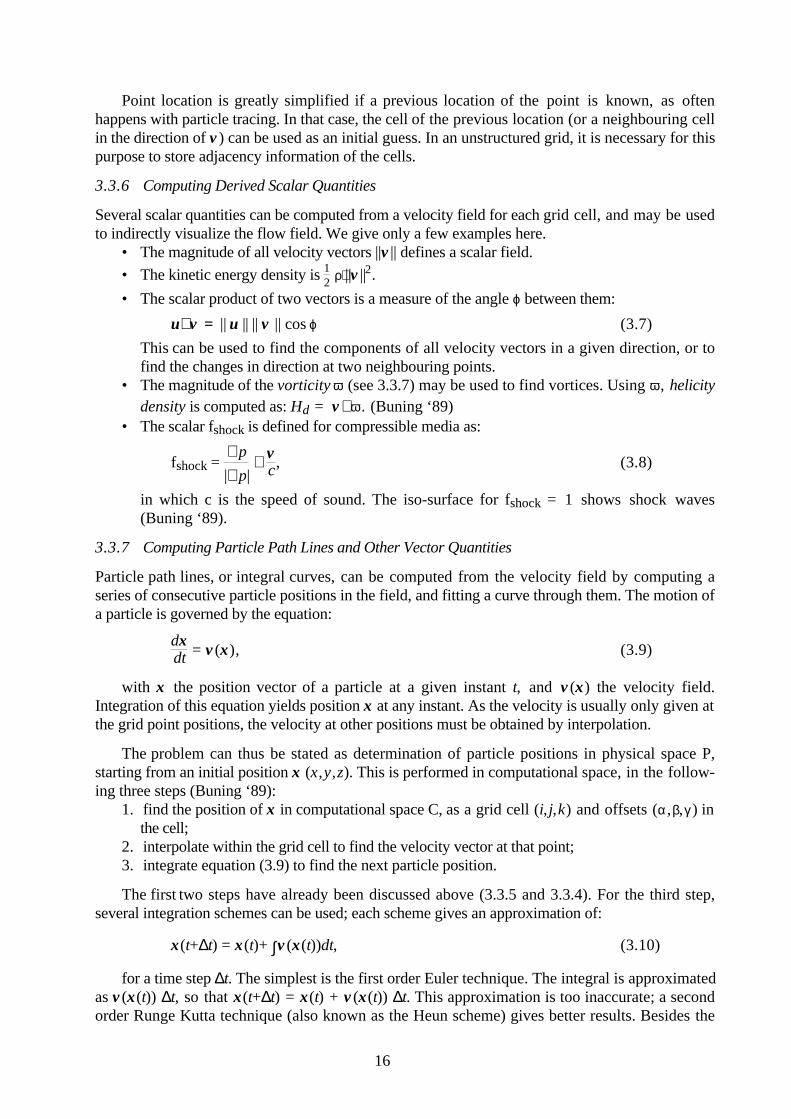
Point location is greatly simplified if a previous location of the point is known, as oftenhappens with particle tracing. In that case, the cell of the previous location (or a neighbouring cellin the direction of v ) can be used as an initial guess. In an unstructured grid, it is necessary for thispurpose to store adjacency information of the cells.

3.3.6 Computing Derived Scalar Quantities

Several scalar quantities can be computed from a velocity field for each grid cell, and may be usedto indirectly visualize the flow field. We give only a few examples here.

• The magnitude of all velocity vectors ||v || defines a scalar field.

• The kinetic energy density is 12 ρ⋅||v ||2.

• The scalar product of two vectors is a measure of the angle ϕ between them:

u⋅ v = || u || || v || cos ϕ (3.7)

This can be used to find the components of all velocity vectors in a given direction, or tofind the changes in direction at two neighbouring points.

• The magnitude of the vorticity ω (see 3.3.7) may be used to find vortices. Using ω , helicitydensity is computed as: Hd = v ⋅ ω . (Buning ‘89)

• The scalar fshock is defined for compressible media as:

fshock = ∇p

|∇p| ⋅ v

c, (3.8)

in which c is the speed of sound. The iso-surface for fshock = 1 shows shock waves(Buning ‘89).

3.3.7 Computing Particle Path Lines and Other Vector Quantities

Particle path lines, or integral curves, can be computed from the velocity field by computing aseries of consecutive particle positions in the field, and fitting a curve through them. The motion ofa particle is governed by the equation:

dxdt = v (x), (3.9)

with x the position vector of a particle at a given instant t, and v (x) the velocity field.Integration of this equation yields position x at any instant. As the velocity is usually only given atthe grid point positions, the velocity at other positions must be obtained by interpolation.

The problem can thus be stated as determination of particle positions in physical space P,starting from an initial position x (x,y,z). This is performed in computational space, in the follow-ing three steps (Buning ‘89):

1. find the position of x in computational space C, as a grid cell (i,j,k) and offsets (α,β,γ ) inthe cell;

2. interpolate within the grid cell to find the velocity vector at that point;3. integrate equation (3.9) to find the next particle position.

The first two steps have already been discussed above (3.3.5 and 3.3.4). For the third step,several integration schemes can be used; each scheme gives an approximation of:

x(t+∆t) = x(t)+ ∫v (x(t))dt, (3.10)

for a time step ∆t. The simplest is the first order Euler technique. The integral is approximatedas v (x(t)) ∆t, so that x(t+∆t) = x(t) + v (x(t)) ∆t. This approximation is too inaccurate; a secondorder Runge Kutta technique (also known as the Heun scheme) gives better results. Besides the

17

velocity at x at instant t, we also use an estimation of the position x* at instant t+∆t; for thispredictor step, we use the Euler method:

x*(t+∆t) = x(t) + v (x(t)) ∆t. (3.11)

Now x*(t+∆t) is used to estimate velocity at t+∆t, and x(t+∆t) is computed in a corrector step:

x(t+∆t) = x(t) + 12 [v (x(t)) + v (x*(t+∆t))]⋅∆t (3.12)

The choice of the time step ∆t also affects accuracy. The optimum time step size is acompromise between accuracy and computational cost. Use of a variable time step, depending onthe gradients in the velocity field, is the best solution. This may be done eg. with ∆t = α/v a, whereα is the number of steps per cell, and v a is the average velocity of the eight surrounding gridpoints.

For visualization of moving particles using animation, particle positions must be known atequal time intervals for each frame, to show velocity information. If particle positions werecomputed with variable time steps, each particle path must be resampled to find positions at equalintervals.

If we are able to compute particle traces, other objects can be easily derived. Stream surfaces(ribbons) can be constructed by fitting surfaces through particle positions, using polygons, or anytype of smooth surface interpolation. Streak lines can be simulated by releasing a continuous flowof particles from a single point. Time lines (-surfaces) can be obtained by releasing a 1D (2D)array of particles at one instant t, and interpolating a curve (surface) through the positions of theseparticles at any given instant.

In a 3D incompressible flow, stream lines are curves that satisfy the equation:

dxu =

dyv =

dzw , (3.13)

where u, v, and w are the velocity components in x-, y-, and z-direction. For a time-independent flow field, the calculation of stream lines amounts to the same as computing particlepaths (Strid et al.’89).

Vorticity is another important vector quantity that can be computed from the velocity field. Forthis computation, the curl of the velocity field must be determined, since vorticity is defined as ω =∇ × v .

3.3.8 Contour Lines and Surfaces

Contour lines can be considered in 2D as intersection curves of a surface defined by a scalarfunction z = f(x,y) and a (horizontal) plane z = c. Usually, no scalar function is known, but a fieldis defined by scalar data values at grid points. To determine contour lines, each grid cell isexamined; if grid values both higher and lower than the contour value are found in a cell, itcontains a part of the contour line. Intersection points can be determined with the edges of the cell,by linear or non-linear interpolation, and these points are connected by line segments, or a smoothcurve is fitted through them. There are several methods to generate contour lines, for differenttypes of grids, interpolations, and orders of curve generation. For an overview, see Sabin (‘85).

In the case of a 3D scalar field, a stack of planes, each with contour lines, may be determinedfor a number of positions in the i-, j- or k-direction of a regular rectangular grid. This can givesome suggestion of 3D contour surfaces, but for properly shaded display other techniques must beapplied. In volume rendering, contours are rendered directly by selective display of voxel values

18

above a certain threshold; surface normals for the lighting calculations are estimated from gradients(Levoy ‘88). This technique gives visually good results, without explicit calculation of the contoursurface.

Another technique often applied in volume visualization is the Marching Cubes algorithm(Lorensen and Cline ‘87). This algorithm finds an explicit polygonal representation of a contoursurface. The principle is as follows:

mark all cells as undonefind a starting cell, and put it into a queuewhile the queue is not empty do

get the next cell from the queueprocess the cell as described belowmark the cell as donefor each of the intersected edges:

put all unmarked neighbour cells sharing the edge into the queue

In a structured grid, the edge-sharing neighbours can be easily found with the cell indices; inan unstructured grid, adjacency information is needed.

For a hexahedral (cubical) cell, all points on the edges with the contour value are determinedby linear interpolation. As there can only be one point per edge, at most 12 points can be found ina cubical cell. Now the intersection of the cell with the contour surface is determined, consisting ofone to four triangles. This is done by encoding the eight vertices of the cell as higher than, orlower than the contour value. The resulting 256 possible different binary code values were reducedto 14 different cases, each corresponding with a distinct configuration of triangles. The binarycode for each cell is used as an index into a table of configurations, which is used to generate theoutput triangles, with the edge intersection points as vertices.

3.4 Flow Field Topology

Since 1987 the analysis and visualization of flow topology has been investigated thoroughly. In anumber of papers, Helman and Hesselink ('87, '88, '89abc, '90, '91) describe the developmentof a system to visualize flow topology. A general classification of flow fields is described byChong et al. ('90). More recently, similar techniques to those of Helman and Hesselink weredescribed. Dickinson ('91) addresses the interactive aspect of flow topology visualization, andGlobus et al. ('91) give detailed information on how to implement a flow topology visualizationmodule.

Flow topology analysis is based on critical point theory, which has been used widely toexamine solution trajectories of ordinary differential equations. The topology of a vector fieldconsists of critical points (where the velocity vector is zero) and integral curves and surfacesconnecting these critical points. Images of a vector field topology display the topologicalcharacteristics of a vector field, without displaying too much redundant information.

The following steps are necessary to analyze and visualize vector field topologies:• the location of the critical points must be calculated• the critical points must be classified• integral curves and surfaces must be calculated

We will discuss these steps in more detail below. It should be noted that, although thetechniques will be described for velocity fields, they can also be applied on any other vector field,such as vorticity fields or pressure gradient fields.

19

3.4.1 Critical points

The positions of the critical points can be found by searching all cells in the flow field. Criticalpoints can only occur in cells where all three (or two, in 2D) components of the vector passthrough zero. The exact position of a critical point can be calculated by interpolation in case of arectangular grid. In case of a curvilinear grid, the position of a critical point can be calculated byrecursively subdividing the cell, or by a numerical method such as Newton iteration (Globus et al.‘91).

Once the critical points have been found, they can be classified. This is done by approximatingthe velocity field in the neighbourhood of the critical point xcp with a first order Taylor expansion.This gives the following formula for the velocity u:

ui ≈ ucp,i + (xj - xcp,j) ∂ui∂xj

. (3.14)

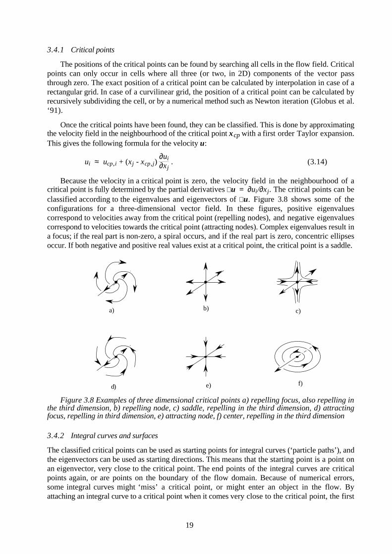
Because the velocity in a critical point is zero, the velocity field in the neighbourhood of acritical point is fully determined by the partial derivatives ∇u = ∂ui/∂xj. The critical points can beclassified according to the eigenvalues and eigenvectors of ∇u. Figure 3.8 shows some of theconfigurations for a three-dimensional vector field. In these figures, positive eigenvaluescorrespond to velocities away from the critical point (repelling nodes), and negative eigenvaluescorrespond to velocities towards the critical point (attracting nodes). Complex eigenvalues result ina focus; if the real part is non-zero, a spiral occurs, and if the real part is zero, concentric ellipsesoccur. If both negative and positive real values exist at a critical point, the critical point is a saddle.

a) b) c)

d) e) f)

Figure 3.8 Examples of three dimensional critical points a) repelling focus, also repelling inthe third dimension, b) repelling node, c) saddle, repelling in the third dimension, d) attractingfocus, repelling in third dimension, e) attracting node, f) center, repelling in the third dimension

3.4.2 Integral curves and surfaces

The classified critical points can be used as starting points for integral curves (‘particle paths’), andthe eigenvectors can be used as starting directions. This means that the starting point is a point onan eigenvector, very close to the critical point. The end points of the integral curves are criticalpoints again, or are points on the boundary of the flow domain. Because of numerical errors,some integral curves might ‘miss’ a critical point, or might enter an object in the flow. Byattaching an integral curve to a critical point when it comes very close to the critical point, the first

20

problem can be solved. To solve the second problem, integral curves that enter an object can berestricted to follow the surface of the object.

In two dimensions, critical points and integral curves completely describe the flow field in aqualitative way. In three dimensions, integral surfaces should also be calculated. Helman andHesselink ('91) describe a way to create some of these integral surfaces. When visualizing theflow around a hemisphere cylinder, they first calculate the topology of the vector field on thesurface of the cylinder. This is, in fact, a two-dimensional topology. Points on the (two-dimensional) integral curves of this topology are used as starting points for a number of three-dimensional integral curves. By tessellating the space between two adjacent integral curves,integral surfaces can be visualized. In this way they are able to show surfaces of separation andreattachment.

4 Presentation Techniques

After data preparation and visualization mapping, the flow data have been cast into a form suitablefor visual presentation. The visualization objects can be transformed into pictures, together withadditional objects such as the environment of the flow, and auxiliary objects such as scales,pointers, colour bars, and numerical or textual annotations. First, we will turn to some aspects ofhuman perception, and relevant visual cues to achieve optimum results for 3D flow visualization.Then we will discuss basic rendering techniques in 4.2, and some more advanced methods in 4.3.

4.1 Human Perception and Depth Cues

In 3D flow data visualization, often complex spatial structures must be shown, and for this a goodorientation in 3-space is essential. Human visual perception can readily extract spatial informationfrom a 2D picture, provided that enough supporting ‘depth cues’ are available. Many depth cuesare related to objects and surfaces, but field data (such as scalar and vector fields) do by nature notcontain objects or surfaces and thus lack these cues. For visualization, extra depth cues must thenbe added, 3D objects and surfaces derived from the fields must be used, or environment geometrymust be exploited to support localization in space.

We will give some examples of important cues for the perception of shapes, depth, andmotion. (For a good introduction and further references, see Thorpe ‘90.)

3D shapes are mainly perceived by their contours, and the directional reflection of light onsurfaces, showing as changes in reflected intensity. Gradual changes indicate a smoothly curvedsurface, while discontinuous changes indicate edges.

Depth or spatial information is perceived in many ways:• perspective: parallel edges converge into the distance; the size of objects decreases linearly

with their distance from the observer;• stereoscopy: the disparity between images seen with two eyes gives a powerful depth

effect, which is independent from other depth cues, and can be applied to virtually everytype of image;

• occlusion: nearer objects cover other, more distant objects;• surface texture density gradients: a continuous density change implies a surface expanding

into depth, a discontinuity is perceived as a contour or an edge;• shadows cast by one object onto the ground or onto other objects give information on

spatial relationships;• distance cues, such as atmospheric haze: the diminishing of colour contrast in the distance;• artificial optical cues, such as depth of field;

21

• user control: if a user is given the possibility to navigate around the 3D display space, toprobe and interrogate the data, this will help the user to build a 3D mental image of the dataspace. An example from flow visualization is the interactive positioning of particle sources(Wavefront Technologies ‘90), and the virtual wind tunnel (Bryson and Levit ‘91), wherethe user can move around in 3D data space, and can use data glove gestures to generateparticle path lines in real time.

Depth ambiguity can easily occur when spatial cues are absent or too weak. This is quitecommon in line drawings (such as arrow plots), which contain no surface information. To supportlocalization of an object floating in space, it can be related to the environment, or to coordinateplanes by showing the object’s coordinates or projection on two or three planes.

Motion can also support depth information. Changes in viewpoint resulting in gradual changesof occlusion relations and perspective, are known as motion parallax; this is readily perceived asextra depth information. The world as perceived by a moving observer has the characteristics of anoptic flow field (Gibson ‘50,’79). A static world ‘flows’ around a moving observer in a standardpattern. If an object is perceived which moves in a way that is different from this pattern, it isdetected to be in motion.

Moving objects can show direction and velocity information. A dense cloud of small objectscan be perceived as a moving texture (Upson et al. ‘89; Van Wijk ‘90b, ‘91), and can be givencertain surface properties to improve localization in space. To preserve velocity information ofmoving objects (particles), the screen update time must be proportional to a simulation time step; inpractice this means that both must be constant. Also, certain precautions must be taken to reducethe disturbing and possibly false effects caused by discretization (see 4.3).

In flow visualization, knowledge of human perception can be used to improve communicatonof spatial and motion information. Below we will show some examples where shape, depth, andmotion cues are consciously applied for this purpose.

4.2 Basic Rendering Techniques

In the visualization mapping stage, visual primitives have been defined to represent the data.Generally speaking, the rendering process consists of four stages: viewing transformations,visible surface determination, lighting calculations, and scan conversion. We will not attempt tosummarize the basic rendering techniques for these primitives. Many techniques for renderinglines, curves, polygons and curved surfaces can be found in any computer graphics textbook (eg.Foley et al. ‘90). Rendering solids is described in Bronsvoort et al. (‘91), and volume rendering inKaufman (‘90). Often, a visualization will consist of a combination of several types of primitives,and therefore it is profitable if a visualization system permits the use of many different primitivesin a single image.

We will concentrate here on the visualization mappings listed in 3.2, and the use of extra depthcues to improve spatial representation of 3D flow fields.

4.2.1 Arrows

Arrows can simply be drawn using only straight lines. In 2D, this can give reasonable results,provided that the arrows are scaled so they do not overlap (figure 4.1).

22

Figure 4.1 2D arrow plot (Bertrand and Tanguy ‘88)

In 3D, rendering arrows is much more complex. Perspective is the only depth cue available; thereis no occlusion, or directional light reflection to assist depth perception. 3D line arrows areambiguous in direction; for example, it is impossible to distinguish between arrows pointingtowards and away from the observer (figure 4.2).

Figure 4.2 Directional ambiguity of 3D arrows

The size of the arrows is determined by three factors: velocity magnitude, direction with respect tothe image plane, and perspective. Also, the display of a full 3D array of arrows very soonbecomes cluttered. Various types of arrows have been devised to minimize cluttering, and toimprove the directional effect (Kroos ‘84), but none of these can fully solve these problems.

An improvement in this respect is to relate the arrows to a plane (figure 4.3), and to showprojections (‘shadows’) of the arrows on the plane. The effect is similar to the use of tufts inexperimental visualization.

23

Figure 4.3 Arrows connected to planes, with projections

The flow field can be sliced, moving a section plane through the field, in the same style asapplied in volume rendering. Observing the gradual changes of the arrows on the plane allows theuser to mentally imagine the entire field.

More spatial cues can be added by drawing arrows as 3D polygonal objects. The occlusion ina visible surface display gives a good depth cue, and reduces directional ambiguity. Also,directional light reflection and shading can be applied, giving some extra information onorientation in space (figure 4.4). But as polygonal arrows are larger, they can lead to an increaseof cluttering.

Figure 4.4 Arrow as 3D object

4.2.2 Curves

Curves, such as stream lines, streak lines, path lines, and contour lines, can be visualized as asequence of short line segments. Again, this gives good results in 2D, but in 3D spatial curves arehard to localize without further depth cues. Also, only a small number of curves can be displayedwithout confusion.

An improvement is showing projections of a curve in the main coordinate planes, allowingmental reconstruction of the 3D shape by the trained observer (figure 4.5).

24

Figure 4.5 Spatial curves with projection in a coordinate plane

Another possibility is to display curves as 3D pipes, allowing occlusion and directional lightreflection. (figure 4.6).

Figure 4.6 Spatial curves rendered as pipes (Geiben and Rumpf ‘91)

It is often desirable to display curves (for example iso-curves or stream lines) on surfaces. Ifthe curves are drawn as lines, their relation with the surface remains weak. A much better result isobtained when the lines are modelled as 3D strips of constant width pasted onto the surface (VanWijk ‘90a). The strips can be rendered transparently, using texture mapping (figure 4.7)

25

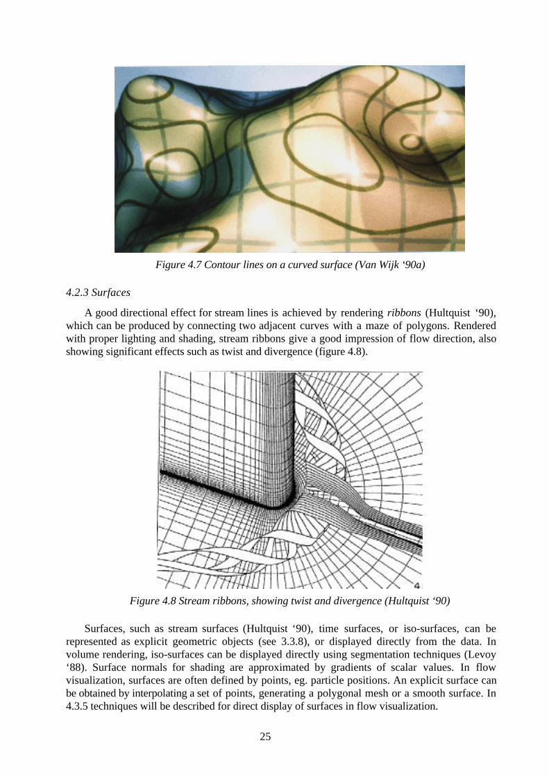
Figure 4.7 Contour lines on a curved surface (Van Wijk ‘90a)

4.2.3 Surfaces

A good directional effect for stream lines is achieved by rendering ribbons (Hultquist ‘90),which can be produced by connecting two adjacent curves with a maze of polygons. Renderedwith proper lighting and shading, stream ribbons give a good impression of flow direction, alsoshowing significant effects such as twist and divergence (figure 4.8).

Figure 4.8 Stream ribbons, showing twist and divergence (Hultquist ‘90)

Surfaces, such as stream surfaces (Hultquist ‘90), time surfaces, or iso-surfaces, can berepresented as explicit geometric objects (see 3.3.8), or displayed directly from the data. Involume rendering, iso-surfaces can be displayed directly using segmentation techniques (Levoy‘88). Surface normals for shading are approximated by gradients of scalar values. In flowvisualization, surfaces are often defined by points, eg. particle positions. An explicit surface canbe obtained by interpolating a set of points, generating a polygonal mesh or a smooth surface. In4.3.5 techniques will be described for direct display of surfaces in flow visualization.

26

Good shape and depth effects can be achieved by many techniques well known in computergraphics. Visible surface display must be applied, and directed lighting and shading with diffuseand specular reflections (see Foley et al. ‘90).

A surface can also be used to display extra data pertaining to it, such as pressure andtemperature. The object colour can be varied according to a scalar quantity, and contour lines canbe shown on the surface (Van Wijk ‘90a; see figure 4.7). Texture mapping allows display ofdirectional information on the surface (Van Wijk ‘91; see 4.3.3). Finally, surfaces can be renderedsemi-transparently, to allow multiple layers of surfaces to be visualized at the same time (figure4.9). A maximum of three layers can be viewed distinctly in this way.

Figure 4.9 Transparent contour surfaces (Gallagher ‘89)

A special use of a surface in flow visualization is the stream polygon (Schroeder et al. ‘91).This is a regular, n-sided polygon, positioned in a flow field, oriented normal to the flowdirection. The polygon can be scaled, sheared, and rotated in response to local strain and rotationin the field, or to other quantities. By sweeping the polygon along a stream line, an n-sidedcylindrical stream tube is obtained. The effects of deformation and sweeping can be combined,yielding a complex cylinder that is twisted and tapered. The surfaces of the polygon and the streamtube can be shaded using directed lighting, and can also show associated data. Figure 4.10 showsan example of this technique.

Figure 4.10 A stream line, ribbon, and stream tube (Schroeder et al. ‘91)

27

4.2.4 Particles

A particle may be rendered as a small-sized object, as a single point, or as a special type ofprimitive that has some characteristics of both. As an object, a circle (in 2D) or a sphere (in 3D)would be an obvious choice. But these objects do not show any changes in orientation. Even withdirected light reflection, a sphere only shows its shape, not its position and orientation in space.To take advantage of changing light reflection as a spatial cue, a flat or elongated shape should beused.

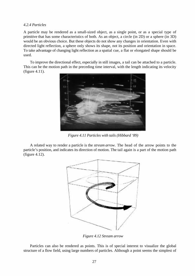
To improve the directional effect, especially in still images, a tail can be attached to a particle.This can be the motion path in the preceding time interval, with the length indicating its velocity(figure 4.11).

Figure 4.11 Particles with tails (Hibbard ‘89)

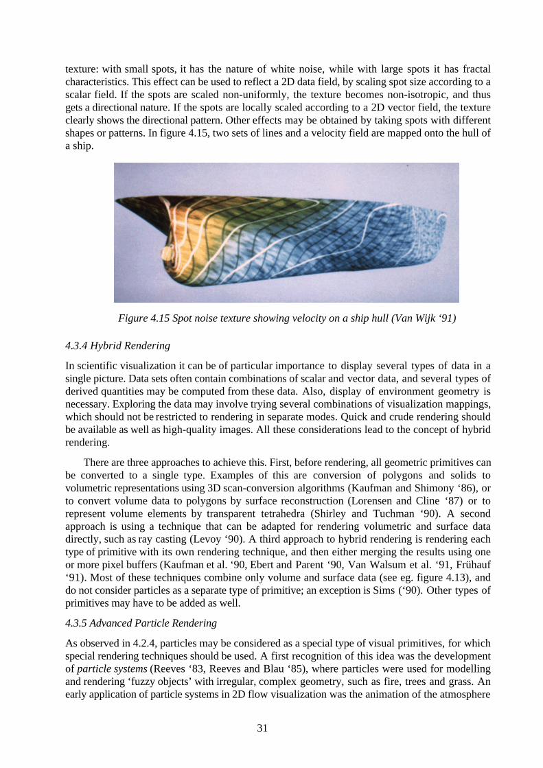
A related way to render a particle is the stream arrow. The head of the arrow points to theparticle’s position, and indicates its direction of motion. The tail again is a part of the motion path(figure 4.12).

Figure 4.12 Stream arrow

Particles can also be rendered as points. This is of special interest to visualize the globalstructure of a flow field, using large numbers of particles. Although a point seems the simplest of

28

all geometric primitives, rendering points is by no means trivial (Van Wijk ‘92). If a point issimply rendered by setting the pixel onto which the point is projected, regardless of its positionwithin the pixel, serious errors occur due to aliasing, caused by the limited resolution of thedisplay screen. We will return to this problem in 4.3.2; we will discuss other particle renderingmethods, including techniques to add extra spatial information to particles in 4.3.5.

4.2.5 Environment Geometry

Display of environment geometry is often desirable in flow visualization, to show the context ofthe particular flow problem studied, and also to support spatial orientation (figure 4.13). Theenvironment can usually be shown as a collection of surfaces or solid objects, allowing the use ofmany spatial cues mentioned before. Techniques for rendering are mainly standard computergraphics methods. But it is important to note that objects of the environment must be displayedtogether with the data, and therefore the rendering technique must be used in combination withother rendering techniques (see 4.3.4).

Figure 4.13 Environment geometry supports spatial orientation (Hin et al.’90)

4.2.6 Volume Rendering

If scalar data fields are associated with flow fields, or when scalar quantities are derived from aflow field (see 3.3.6), volume rendering techniques can be used to visualize these data (for asurvey of volume rendering techniques, see Kaufman ‘90). In volume rendering, a scalar datafield (eg. a density field) is usually considered as a regular 3D array of cubical volume elements(voxels), with one scalar data item associated with each volume element. A segmentation is madeof the data, by selecting only the voxels that satisfy a selection criterion (such as a given minimumscalar value), or by applying other 3D image segmentation techniques. The selected voxels arethen projected onto the screen and rendered using special techniques for visible surface display andshading.

Although in volume rendering surfaces are often displayed directly, iso-surfaces can also begenerated explicitly from volume data as a polygon mesh, using the method described in 3.3.8.

29

If a surface is defined that intersects the data volume, the scalar values on the surface can bedetermined by interpolation, and these can be shown using colour coding and iso-lines. The samecan be done with a surface at the model boundary, such as an airplane wing or a ship hull. Thesurface may be shaded using directed light reflection, to provide good spatial cues.

Plane sections are often used in volume visualization to inspect a 3D data volume. This can beachieved by moving a plane through the volume and watching the changing patterns projected ontothe section plane, to build a mental image of the whole field.

4.3 Special Rendering Techniques

4.3.1 Animation

Animation can be used for many purposes in flow visualization. As mentioned before, particlemotion can be very effectively visualized using animation sequences. The velocity of particles canbe directly visualized, provided that particle positions are known at constant intervals, and theupdate time of the images on the screen is also constant.

Animations can either be produced in real time, or simply by playback of a series of pre-computed images (frames). In real time animation, rendering of each frame is done during display.This has the advantage that the animation may be interactively controlled by the user. Adisadvantage is that the screen update time usually depends on image complexity (for example, thenumber of visible particles), which may vary per frame. Also, the choice of rendering techniquesis severely restricted. If we want to achieve the update rate of at least 5-10 frames per secondrequired to produce the illusion of motion, only the most simple and fast rendering techniques canbe used. To accelerate the process, some parameters such as particle paths can be pre-computed,but this reduces the possibilities for interactive control.

Pre-computed frames may be displayed one at a time and recorded on a video tape, or playedback directly on the screen. In the latter case, all frames must be displayed from main memory, astransfer from disk is too slow. The size of main memory thus restricts the length of an on-screenanimation. As the screen update rate is independent of the contents of the frames, playback speedcan be constant. Interactive control of most viewing parameters (such as viewing direction) orpositioning of particle sources is not possible.

A problem in animated flow visualization is the number of frames needed to get a clear view ofthe flow patterns. For an unsteady flow, a new velocity field must be computed for each frame,and new particle positions in this field. For one minute of animation, this must be performed forabout 1500 frames. With a steady flow, particle paths are derived from a single velocity field; asthe paths do not change in time, cyclic animation can be applied (Van Wijk ‘90b; Stolk and VanWijk ‘91), showing a smooth motion by continuously repeated display of a limited number offrames (typically 10-30).

Animation can be used for many other purposes in flow visualization. A changing viewpoint(or a rotating object) provides a powerful depth cue (motion parallax), that is quite independent ofother cues, and can be used to resolve depth ambiguity even in wire frame drawings, such asarrow plots. Other applications of animation are inspection by moving a section plane through anarea, or changing iso-values.

4.3.2 Aliasing and Anti-Aliasing

An important visual effect caused by the discrete nature of the display screen is known as aliasing.It is obvious from the jagged edges and silhouettes, Moiré patterns, irregular and granulartextures, and missing small details. In animation, the effects are even more disturbing.

30

Aliasing can be explained from signal theory (Blinn ‘89; Foley et al. ‘90). The colour of apixel is often determined by taking only one point sample. Better results can be achieved byconsidering a pixel as a small area to which one colour is assigned, and determining this colourfrom all objects that are visible within the pixel area. The contributions of the objects can beestimated by taking several point samples for one pixel (supersampling), or by geometriccalculations (area sampling). The contributions are then combined to determine the colour of thepixel.

When combining several samples to determine the colour for a given pixel, digital low-passfiltering can be applied. The samples are weighted according to a filter function, which specifiesthe weights dependent on the distance of a sample point to the pixel center. From the samplevalues, a weighted average is then computed.

Analog to the spatial aliasing described above, temporal aliasing is caused by taking only onepoint sample for each time step. This results in jerky motion, flicker, ‘strobing’ effects, and evenfalse movements that are unacceptable in animated flow visualization.

To reduce this, the time interval between two frames should be considered. For a movingparticle, this would be its trajectory over the time interval. Smooth motion can then be achievedusing digital filtering, using this trajectory or a number of samples on it. The result is a blurredimage of the moving particle, extended in the direction of motion, with a fuzzy shape. This effect,known as motion blur, produces smooth motion without false effects (Sims ‘90).

4.3.3 Texture Synthesis and Texture Mapping

A texture is a pattern that can be mapped onto a surface, and used to modify the surface’s opticalproperties. The most common form is modification of surface colour, resulting in a colouredpattern pasted onto the surface; other properties, such as reflectivity, transparency, or normalvector direction, can also be modified by texture (Heckbert ‘86). In texture mapping, obviousadverse effects are caused by the aliasing problems mentioned above, and therefore digital filteringis usually necessary to obtain good results (figure 4.14).

Figure 4.14 Aliasing in texture mapping - left: with point sampling; right: with digitalfrequency filtering (Heckbert ‘86)

Existing images, such as digitized photographs, can be used as texture, but texture can also begenerated synthetically. Techniques for synthesis of texture has been mainly developed to achievenaturalistic effects: to suggest certain materials or rough surfaces. As a primitive for visualization,texture has been little explored, but some of its potential is shown by Van Wijk (‘90a, ‘91).

A good example is the synthesis of spot noise, a type of texture especially designed for datavisualization (Van Wijk ‘91). Spot noise is a stochastic texture generated as an addition of manyrandomly distributed and weighted 2D patterns (spots). The texture can be globally and locallycontrolled by varying the attributes of the spots. The spot size controls the granularity of the

31

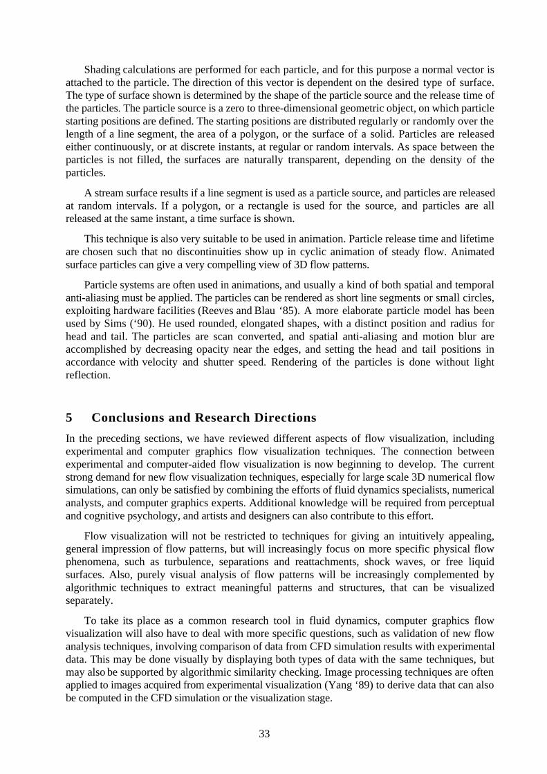
texture: with small spots, it has the nature of white noise, while with large spots it has fractalcharacteristics. This effect can be used to reflect a 2D data field, by scaling spot size according to ascalar field. If the spots are scaled non-uniformly, the texture becomes non-isotropic, and thusgets a directional nature. If the spots are locally scaled according to a 2D vector field, the textureclearly shows the directional pattern. Other effects may be obtained by taking spots with differentshapes or patterns. In figure 4.15, two sets of lines and a velocity field are mapped onto the hull ofa ship.

Figure 4.15 Spot noise texture showing velocity on a ship hull (Van Wijk ‘91)

4.3.4 Hybrid Rendering

In scientific visualization it can be of particular importance to display several types of data in asingle picture. Data sets often contain combinations of scalar and vector data, and several types ofderived quantities may be computed from these data. Also, display of environment geometry isnecessary. Exploring the data may involve trying several combinations of visualization mappings,which should not be restricted to rendering in separate modes. Quick and crude rendering shouldbe available as well as high-quality images. All these considerations lead to the concept of hybridrendering.

There are three approaches to achieve this. First, before rendering, all geometric primitives canbe converted to a single type. Examples of this are conversion of polygons and solids tovolumetric representations using 3D scan-conversion algorithms (Kaufman and Shimony ‘86), orto convert volume data to polygons by surface reconstruction (Lorensen and Cline ‘87) or torepresent volume elements by transparent tetrahedra (Shirley and Tuchman ‘90). A secondapproach is using a technique that can be adapted for rendering volumetric and surface datadirectly, such as ray casting (Levoy ‘90). A third approach to hybrid rendering is rendering eachtype of primitive with its own rendering technique, and then either merging the results using oneor more pixel buffers (Kaufman et al. ‘90, Ebert and Parent ‘90, Van Walsum et al. ‘91, Frühauf‘91). Most of these techniques combine only volume and surface data (see eg. figure 4.13), anddo not consider particles as a separate type of primitive; an exception is Sims (‘90). Other types ofprimitives may have to be added as well.

4.3.5 Advanced Particle Rendering

As observed in 4.2.4, particles may be considered as a special type of visual primitives, for whichspecial rendering techniques should be used. A first recognition of this idea was the developmentof particle systems (Reeves ‘83, Reeves and Blau ‘85), where particles were used for modellingand rendering ‘fuzzy objects’ with irregular, complex geometry, such as fire, trees and grass. Anearly application of particle systems in 2D flow visualization was the animation of the atmosphere

32

of Jupiter in the film 2010 (Yaeger et al. ‘86). A more recent example was shown by Van Wijk(‘90b).

A particle system is a collection of particles representing a fuzzy object. The particles have acertain life cycle: they are born, have a limited lifetime, and die; during the lifetime, variousattributes such as motion dynamics (position, speed, motion direction), and visual appearance(shape, size, colour, reflectivity, transparency) may vary as a function of time. They can also havecertain collective properties, which allows modelling of structured objects. In flow visualization,the motion dynamics of the particles is determined by a flow field, but the other attributes can beused to convey spatial information or to visualize associated data.

The rendering of the particles depends on their attributes. If particles are considered as lightemitting points, then rendering is simply done by adding intensities of particles projected onto asingle pixel, without any visibility calculations. These particles do not carry much spatialinformation. If the particles are considered as light-reflecting, shading calculations must beperformed; also, self-shadowing (shadows cast by one particle onto others) is desirable as a depthcue. Precise shading and shadowing calculations are prohibitive for very large numbers (more than106), but then probabilistic shading models can be used. The position and orientation of a particledetermine the probability that it is lighted directly, and ambient, diffuse, and specular reflectioncomponents are assigned, based on these probabilities (Reeves and Blau ‘85). The particles aredepth sorted for visibility, and rendered in back-to-front order. Transparency can thus be achievedby blending the colours of the particles appearing in the same pixel.

To display more spatial information, a particle can be modelled as a very small surface elementthat reflects directed light; it is then called a surface-particle (Stolk and Van Wijk ‘91). This has theadditional advantage that a (large) collection of surface-particles may show a stream surface or atime surface (or indeed, any surface moving with and deformed by the flow), withoutdetermination of explicit surface geometry. As an example, a stream surface consisting of surface-particles is shown in figure 4.16.

Figure 4.16 Surface-particles (Stolk and Van Wijk ‘91)

33

Shading calculations are performed for each particle, and for this purpose a normal vector isattached to the particle. The direction of this vector is dependent on the desired type of surface.The type of surface shown is determined by the shape of the particle source and the release time ofthe particles. The particle source is a zero to three-dimensional geometric object, on which particlestarting positions are defined. The starting positions are distributed regularly or randomly over thelength of a line segment, the area of a polygon, or the surface of a solid. Particles are releasedeither continuously, or at discrete instants, at regular or random intervals. As space between theparticles is not filled, the surfaces are naturally transparent, depending on the density of theparticles.

A stream surface results if a line segment is used as a particle source, and particles are releasedat random intervals. If a polygon, or a rectangle is used for the source, and particles are allreleased at the same instant, a time surface is shown.

This technique is also very suitable to be used in animation. Particle release time and lifetimeare chosen such that no discontinuities show up in cyclic animation of steady flow. Animatedsurface particles can give a very compelling view of 3D flow patterns.

Particle systems are often used in animations, and usually a kind of both spatial and temporalanti-aliasing must be applied. The particles can be rendered as short line segments or small circles,exploiting hardware facilities (Reeves and Blau ‘85). A more elaborate particle model has beenused by Sims (‘90). He used rounded, elongated shapes, with a distinct position and radius forhead and tail. The particles are scan converted, and spatial anti-aliasing and motion blur areaccomplished by decreasing opacity near the edges, and setting the head and tail positions inaccordance with velocity and shutter speed. Rendering of the particles is done without lightreflection.

5 Conclusions and Research Directions

In the preceding sections, we have reviewed different aspects of flow visualization, includingexperimental and computer graphics flow visualization techniques. The connection betweenexperimental and computer-aided flow visualization is now beginning to develop. The currentstrong demand for new flow visualization techniques, especially for large scale 3D numerical flowsimulations, can only be satisfied by combining the efforts of fluid dynamics specialists, numericalanalysts, and computer graphics experts. Additional knowledge will be required from perceptualand cognitive psychology, and artists and designers can also contribute to this effort.

Flow visualization will not be restricted to techniques for giving an intuitively appealing,general impression of flow patterns, but will increasingly focus on more specific physical flowphenomena, such as turbulence, separations and reattachments, shock waves, or free liquidsurfaces. Also, purely visual analysis of flow patterns will be increasingly complemented byalgorithmic techniques to extract meaningful patterns and structures, that can be visualizedseparately.

To take its place as a common research tool in fluid dynamics, computer graphics flowvisualization will also have to deal with more specific questions, such as validation of new flowanalysis techniques, involving comparison of data from CFD simulation results with experimentaldata. This may be done visually by displaying both types of data with the same techniques, butmay also be supported by algorithmic similarity checking. Image processing techniques are oftenapplied to images acquired from experimental visualization (Yang ‘89) to derive data that can alsobe computed in the CFD simulation or the visualization stage.

34

Before they can be used as reliable research tools, the visualization techniques themselvesmust also be carefully tested and validated. As we have seen in the previous sections, visualizationinvolves a sequence of many processing steps, where approximations are frequently used andnumerical errors can easily occur. Even at the visual level, interpolation artifacts, aliasing, orcontradictory depth cues may cause incorrect interpretations.

An important issue following development of visualization techniques, is the design andimplementation of flow visualization systems. Here, there are many other issues that should beexplored further, such as distributed processing, data management, standardization of dataformats, and user interaction. Many styles and modes of interaction are possible, depending on theextent of control of the visualization (and flow simulation) process (Hearn and Baker ‘91). Theinteraction style provided by general purpose visualization systems such as AVS (Upson et al ‘89)and apE (Dyer ‘90), enabling the user to construct data flow networks, allows manipulation of thevisualization process rather than the displayable objects representing the data. The concept of‘direct manipulation’ of the data needs clarification; desirable facilities would certainly includeinteractive probing and interrogation (Speray and Kennon ‘90).

Research in computer graphics flow visualization is still in its early stages, and especially 3Dflow field visualization is still very much an open problem. At present, this is one of the greatchallenges of scientific visualization. This calls for a cooperative effort in the development of newtechniques at all stages of the flow visualization process.

Acknowledgements

We would like to thank Delft Hydraulics, the Netherlands Energy Research Foundation (ECN)and the High-Speed Laboratory of the Department of Aerospace Engineering at Delft University ofTechnology for their cooperation and for permission to use several illustrations. Also, we want toexpress thanks to Andrea Hin, Arthur Mynett, Guus Segal, and Jack van Wijk for their valuablecriticism of earlier versions of this paper. Finally, we thank the editor Heinrich Müller for hisencouragement and patience.

References

Batchelor, G.K. (1967) An Introduction to Fluid Dynamics, Cambridge University PressBertrand, F.H., P.A. Tanguy (1988) Graphical Representation of Two-dimensional Fluid Flow

by Stream Vectors, Communications in Applied Numerical Methods 4, pp. 213-217Blinn, J.F.(1989) What We Need Around Here Is More Aliasing / Return of the Jaggy, IEEE

Computer Graphics and Applications 9(1), pp. 75-79, and 9(2), pp. 82-89Briscolini, M., P. Santangelo (1991) Animation of Computer Simulations of Two-Dimensional

Turbulence and Three-Dimensional Flows, IBM Journal of Research and Development”35(1/2), pp. 119-138

Bronsvoort, W.F., F.W. Jansen, F.H. Post (1991) Design and Display of Solid Models, InAdvances in Computer Graphics VI, G. Garcia, I. Herman (eds.), Springer Verlag, pp. 1-57

Bryson, S., C. Levit (1991) The Virtual Windtunnel: An Environment for the Exploration ofThree-Dimensional Unsteady Flows, In Proceedings Visualization ‘91, G.M. Nielson, L.Rosenblum (eds.), IEEE Computer Society Press, pp. 17-24

Buning, P.G.(1989) Numerical Algorithms in CFD Post-Processing, von Karman Institute forFluid Dynamics, Lecture Series 1989-07

Chen, H.H., T.S. Huang (1988) A Survey of Construction and Manipulation of Octrees,Computer Vision, Graphics and Image Processing 43, pp. 403-431

Chong, M.S., A.E. Perry, B.J. Cantwell (1990) A General Classification of Three-dimensionalFlow Fields, Physics of Fluids A 2(5), pp. 765-777

Dickinson, R.R. (1991) Interactive Analysis of the Topology of 4D Vector Fields, IBM Journal ofResearch and Development 35(1/2), pp. 59-66

35

Dyer, D.S. (1990) A Dataflow Toolkit for Visualization, IEEE Computer Graphics andApplications 10(4), pp. 60-69

Dyke, M. van (1982) An Album of Fluid Motion, The Parabolic PressEbert, D.S, R.E. Parent (1990) Rendering and Animation of Gaseous Phenomena by Combining

Fast Volume and Scanline A-buffer Techniques, Proceedings Siggraph ‘90, ComputerGraphics 24(4), pp. 357-366

Foley, J.D., A. van Dam, S. Feiner, J. Hughes (1990) Computer Graphics: Principles andPractice, second edition, Addison-Wesley Publishing Company

Frühauf, M. (1991) Combining Volume Rendering with Line and Surface Rendering, InEurographics ‘91, F.H. Post, W. Barth (eds.), North Holland, pp. 21-32

Gallagher, R.S. (1991) Span Filtering: an Optimization Scheme for Volume Visualization of LargeFinite Element Models, In Proceedings Viualization ‘91, G.M. Nielson, L. Rosenblum (eds.),IEEE Computer Society Press, pp. 68-75

Gallagher, R.S., J.C. Nagtegaal (1989) An Efficient 3-D Visualization Technique for FiniteElement Models and Other Coarse Volumes, Proceedings Siggraph ‘89, Computer Graphics23(3), pp. 185-194

Geiben M., M. Rumpf (1991), Visualization of Finite Elements and Tools for NumericalAnalysis, In Advances in Scientific Visualization, F.H. Post, A.J.S. Hin (eds.), SpringerVerlag (to appear in 1992)

Gibson, J.J.(1950), The Perception of the Visual World, Houghton Mifflin Co.Gibson, J.J.(1979), The Ecological Approach to Visual Perception, Houghton Mifflin Co.Globus, A., C. Levit, T. Lasinski (1991) A Tool for Visualizing the Topology of Three-

Dimensional Vector Fields, In Proceedings of Viualization ‘91, G.M. Nielson, L. Rosenblum(eds.), IEEE Computer Society Press, pp. 33-40

Haber, R.B., D.A. McNabb (1990), Visualization Idioms: A Conceptual Model for ScientificVisualization Systems, In Visualization in Scientific Computing, G.M. Nielson, B. Shriver,L.J. Rosenblum (eds.), IEEE Computer Society Press, pp. 74-92

Hearn, D.D., P. Baker (1991) Scientific Visualization, Eurographics ‘91 Tutorial Notes no. 6,Eurographics Technical Report Series EG91 TN6.

Heckbert, P.S. (1986) Survey of Texture Mapping, IEEE Computer Graphics and Applications6(11), pp.56-67

Helman, J., L. Hesselink (1989a) Automated Analysis of Fluid Flow Topology, 3D Visualizationand Display Technologies (Proc. SPIE) 1083, SPIE, Bellingham, Wash., pp. 825-835

Helman, J., L. Hesselink (1989b) Analysis and Visualization of Flow Topology in NumericalData Sets, IUTAM Symposium on “Topological Fluid Mechanics”, Cambridge, England

Helman, J., L. Hesselink (1989c) Representation and Display of Vector Field Topology in FluidFlow Data Sets, IEEE Computer 22(8), pp. 27-36

Helman, J., L. Hesselink (1990) Surface Representations of Two- and Three-Dimensional FluidFlow Topology, In Proceedings Visualization ‘90, A. Kaufman (ed.), IEEE Computer SocietyPress, pp. 6-13

Helman, J., L. Hesselink (1991) Visualizing Vector Field Topology in Fluid Flows, IEEEComputer Graphics and Applications 11(3), pp. 36-46

Hesselink, L., J. Helman (1987) Evalution of Flow Topology from Numerical Data, InvitedAIAA-paper, 87-1181-CP

Hesselink, L., J. Helman, K. Wu (1988) Visualization and Interpretation of 3-D Scientific DataSets, ICALEO ‘88-Conference, Santa Clara CA

Hibbard, W., D. Santek (1989) Visualizing Large Data Sets in the Earth Sciences, IEEE Computer22(8), pp. 53-57

Hin, A.J.S., E. Boender, F.H. Post (1990) Visualization of 3D Scalar Fields using Ray Casting,In Proceedings of the Eurographics Workshop on Visualization in Scientific Computing, M.Grave, Y. Le Lous (eds.), to be published by Springer Verlag

Hultquist, J.P.M.(1990) Interactive Numeric Flow Visualization Using Stream Surfaces,Computing Systems in Engineering, 1(2-4), pp. 349-353

Kaufman, A., ed. (1990) Volume Visualization, IEEE Computer Society PressKaufman, A., E. Shimony (1986) 3D Scan Conversion Algorithms for Voxel-Based Graphics, In

Proceedings 1986 Workshop on Interactive 3D Graphics, F. Crow, S.M. Pizer (eds.), ACM,pp. 45-75

36

Kaufman, A., R. Yagel, D. Cohen (1990) Intermixing Surface and Volume Rendering, In 3DImaging in Medicine: Algorithms, Systems, Applications, K.H. Höhne, H. Fuchs, S.M. Pizer(eds.), Springer Verlag, pp. 217-227

Kroos, K.A.(1984) Computer Graphics Flow Visualization Techniques for Three-DimensionalFlow Visualization, In Frontiers in Computer Graphics, T.L. Kunii (ed.), Springer Verlag,pp. 129-145

Levoy, M. (1988) Display of Surfaces from Volume Data, IEEE Computer Graphics andApplications 8(3), pp. 29-37

Levoy, M. (1990) A Hybrid Ray Tracer for Rendering Polygons and Volume Data, IEEEComputer Graphics and Applications 10(2), pp. 33-40

Lorensen, W.E., H.E. Cline (1987) Marching Cubes: a High Resolution 3D Surface ConstructionAlgorithm, Proceedings Siggraph ‘87, Computer Graphics 21(4), pp. 163-169

Merzkirch, W. (1987) Flow Visualisation, second edition, Academic Press Inc.Nielson, G.M., B.S. Shriver, L.J. Rosenblum, eds. (1990) Visualization in Scientific

Computing, IEEE Computer Socitety PressPapathomas, T.V., J.A. Schiavone, B. Julesz (1988), Applications of Computer Graphics to the

Visualization of Meteorological Data, Proceedings Siggraph ‘88, Computer Graphics 22(4),pp. 327-335

Reeves, W.T.(1983), Particle Systems - a Technique for Modelling a Class of Fuzzy Objects,ACM Transactions on Graphics 2(2), pp. 91-108

Reeves, W.T., R. Blau (1985) Approximate and Probabilistic Algorithms for Shading andRendering Structured Particle Systems, Proceedings Siggraph ‘85, Computer Graphics 19(3),pp. 313-322

Sabin, M.A. (1985) Contouring - the State of the Art, in Fundamental Algorithms for ComputerGraphics, R.A. Earnshaw (ed.), Springer Verlag, pp. 411-482

Samet, H. (1990) The Design and Analysis of Spatial Data Structures and Applications of SpatialData Structures, Addison-Wesley Publishing Company

Schroeder, W.J., C.R. Volpe, W.E. Lorensen (1991) The Stream Polygon: a Technique for 3DVector Field Visualization, In Proceedings Visualization ‘91, G.M. Nielson, L. Rosenblum(eds.), IEEE Computer Society Press, pp. 126-132

Sims, K.(1990) Particle Animation and Rendering Using Data Parallel Computation, ProceedingsSiggraph ‘90, Computer Graphics 24(4), pp. 405-413

Shirley, P., A. Tuchman (1990) A Polygonal Approximation to Direct Scalar Volume Rendering,Proceedings San Diego Workshop on Volume Visualization, Computer Graphics 24(5), pp.63-69

Speray, D., S. Kennon (1990) Volume Probes: Interactive Data Exploration on Arbitrary Grids,Proceedings San Diego Workshop on Volume Visualization, Computer Graphics 24(5), pp.5-12

Stolk, J., J.J. van Wijk (1991) Surface-particles for 3D Flow Visualization, In Advances inScientific Visualization, F.H. Post, A.J.S. Hin (eds.), Springer Verlag (to appear in 1992)

Strid, T., A. Rizzi, J. Oppelstrup (1989), Development and Use of some Flow VisualizationAlgorithms, von Karman Institute for Fluid Dynamics, Lecture Series 1989-07

Thorpe, S.J. (1990), Image Processing by the Human Visual System, Eurographics ‘90 TutorialNotes no. 4, Eurographics Technical Report Series EG90 TN4

Upson, C. et al. (1989), The Application Visualization System: a Computational Environment forScientific Visualization, IEEE Computer Graphics and Applications 9(4), pp. 30-42

Upson, C., M. Keeler (1988) V-Buffer: Visible Volume Rendering, Computer Graphics 22(4),pp. 59-64

Walsum, T. van, A.J.S. Hin, J. Versloot, F.H. Post (1991) Efficient Hybrid Rendering ofVolume Data and Polygons, In Advances in Scientific Visualization, F.H.Post, A.J.S. Hin(eds.), Springer Verlag (to appear in 1992)

Wavefront Technologies (1990) The Data Visualizer Version 1.0 Users Guide, 1990Wijk, J.J. van (1990a) Rendering Lines on Curved Surfaces, In Proceedings of the Eurographics

Workshop on Visualization in Scientific Computing, M. Grave, Y. Le Lous (eds.), to bepublished by Springer Verlag

Wijk, J.J. van (1990b) A Raster Graphics Approach to Flow Visualization, In Eurographics ‘90 ,C.E. Vandoni, D.A. Duce (eds.), pp. 251-259

Wijk, J.J. van (1991) Spot Noise - Texture Synthesis for Data Visualization, ProceedingsSiggraph ‘91, Computer Graphics 25(4), pp. 309-318

37

Wijk, J.J. van (1992) Rendering Surface Particles, paper submitted for publication,Yaeger, L., C. Upson, R. Myers (1986) Combining Physical and Visual Simulation - Creation of

the Planet Jupiter for the Film "2010", Proceedings Siggraph ‘86, Computer Graphics 20(4),pp. 85-93

Yang, W.J., ed. (1989) Handbook of Flow Visualization, Hemisphere Publishing Corporation