Fluid Mechanics forChemical Engineers

Second Edition

with Microfluidics and CFD

The Prentice Hall International Series in the Physical and

Chemical Engineering Sciences had its auspicious beginning in

1956 under the direction of Neal R. Amundsen. The series comprises the

most widely adopted college textbooks and supplements for chemical

engineering education. Books in this series are written by the foremost

educators and researchers in the field of chemical engineering.

Visit informit.com/ph/physandchem

for a complete list of available publications.

Prentice Hall International Series in the Physical and Chemical Engineering Sciences

FLUID MECHANICS FOR

CHEMICAL ENGINEERS

Second Edition

with Microfluidics and CFD

JAMES O. WILKESDepartment of Chemical Engineering

The University of Michigan, Ann Arbor, MI

with contributions by

STACY G. BIRMINGHAM: Non-Newtonian FlowMechanical Engineering Department

Grove City College, PA

BRIAN J. KIRBY: MicrofluidicsSibley School of Mechanical and Aerospace Engineering

Cornell University, Ithaca, NY

COMSOL (FEMLAB): Multiphysics ModelingCOMSOL, Inc., Burlington, MA

CHI-YANG CHENG: Computational Fluid Dynamics and FlowLabFluent, Inc., Lebanon, NH

Prentice Hall Professional Technical ReferenceUpper Saddle River, NJ • Boston • Indianapolis • San FranciscoNew York • Toronto • Montreal • London • Munich • Paris • MadridCapetown • Sydney • Tokyo • Singapore • Mexico City

are claimed as trademarks. Where those designations appear in this book, and the pub-lisher was aware of a trademark claim, the designations have been printed with initialcapital letters or in all capitals.

The author and publisher have taken care in the preparation of this book, but makeno expressed or implied warranty of any kind and assume no responsibility for errors oromissions. No liability is assumed for incidental or consequential damages in connectionwith or arising out of the use of the information or programs contained herein.

The publisher offers excellent discounts on this book when ordered in quantity for bulkpurchases or special sales, which may include electronic versions and/or custom coversand content particular to your business, training goals, marketing focus, and brandinginterests.For more information, please contact:

U.S. Corporate and Government Sales(800) 382–3419corpsales@pearsontechgroup.com

For sales outside the U.S., please contact:International Salesinternational@pearsoned.com

Visit us on the Web: www.phptr.com

Library of Congress Cataloging-in-Publication DataWilkes, James O.Fluid mechanics for chemical engineers, 2nd ed., with microfluidics

and CFD/James O. Wilkes.p. cm.

Includes bibliographical references and index.ISBN 0–13–148212–2 (alk. paper)1. Chemical processes. 2. Fluid dynamics. I. Title.TP155.7.W55 2006660’.29–dc22 2005017816

Copyright c© 2006 Pearson Education, Inc.

All rights reserved. Printed in the United States of America. This publication is protectedby copyright, and permission must be obtained from the publisher prior to any prohibitedreproduction, storage in a retrieval system, or transmission in any form or by any means,electronic, mechanical, photocopying, recording, or likewise. For information regardingpermissions, write to:

Pearson Education, Inc.Rights and Contracts DepartmentOne Lake StreetUpper Saddle River, NJ 07458

Many of the designations used by manufacturers and sellers to distinguish their products

ISBN 0-13-148212-2

Printingth ber 2012Text printed in the United States on recycled paper at Courier Westford in Westford, Massachusetts

.

Octo8

Dedicated to the memory of

Terence Robert Corelli Fox

Shell Professor of Chemical EngineeringUniversity of Cambridge, 1946–1959

This page intentionally left blank

CONTENTS

PREFACE xv

PART I—MACROSCOPIC FLUID MECHANICS

CHAPTER 1—INTRODUCTION TO FLUID MECHANICS

1.1 Fluid Mechanics in Chemical Engineering 31.2 General Concepts of a Fluid 31.3 Stresses, Pressure, Velocity, and the Basic Laws 51.4 Physical Properties—Density, Viscosity, and Surface Tension 101.5 Units and Systems of Units 21

Example 1.1—Units Conversion 24Example 1.2—Mass of Air in a Room 25

1.6 Hydrostatics 26Example 1.3—Pressure in an Oil Storage Tank 29Example 1.4—Multiple Fluid Hydrostatics 30Example 1.5—Pressure Variations in a Gas 31Example 1.6—Hydrostatic Force on a Curved Surface 35Example 1.7—Application of Archimedes’ Law 37

1.7 Pressure Change Caused by Rotation 39Example 1.8—Overflow from a Spinning Container 40

Problems for Chapter 1 42

CHAPTER 2—MASS, ENERGY, AND MOMENTUM BALANCES

2.1 General Conservation Laws 552.2 Mass Balances 57

Example 2.1—Mass Balance for Tank Evacuation 582.3 Energy Balances 61

Example 2.2—Pumping n-Pentane 652.4 Bernoulli’s Equation 672.5 Applications of Bernoulli’s Equation 70

Example 2.3—Tank Filling 762.6 Momentum Balances 78

Example 2.4—Impinging Jet of Water 83Example 2.5—Velocity of Wave on Water 84Example 2.6—Flow Measurement by a Rotameter 89

vii

viii Contents

2.7 Pressure, Velocity, and Flow Rate Measurement 92Problems for Chapter 2 96

CHAPTER 3—FLUID FRICTION IN PIPES

3.1 Introduction 1203.2 Laminar Flow 123

Example 3.1—Polymer Flow in a Pipeline 1283.3 Models for Shear Stress 1293.4 Piping and Pumping Problems 133

Example 3.2—Unloading Oil from a TankerSpecified Flow Rate and Diameter 142

Example 3.3—Unloading Oil from a TankerSpecified Diameter and Pressure Drop 144

Example 3.4—Unloading Oil from a TankerSpecified Flow Rate and Pressure Drop 147

Example 3.5—Unloading Oil from a TankerMiscellaneous Additional Calculations 147

3.5 Flow in Noncircular Ducts 150Example 3.6—Flow in an Irrigation Ditch 152

3.6 Compressible Gas Flow in Pipelines 1563.7 Compressible Flow in Nozzles 1593.8 Complex Piping Systems 163

Example 3.7—Solution of a Piping/Pumping Problem 165Problems for Chapter 3 168

CHAPTER 4—FLOW IN CHEMICAL ENGINEERING EQUIPMENT

4.1 Introduction 1854.2 Pumps and Compressors 188

Example 4.1—Pumps in Series and Parallel 1934.3 Drag Force on Solid Particles in Fluids 194

Example 4.2—Manufacture of Lead Shot 2024.4 Flow Through Packed Beds 204

Example 4.3—Pressure Drop in a Packed-Bed Reactor 2084.5 Filtration 2104.6 Fluidization 2154.7 Dynamics of a Bubble-Cap Distillation Column 2164.8 Cyclone Separators 2194.9 Sedimentation 2224.10 Dimensional Analysis 224

Example 4.4—Thickness of the Laminar Sublayer 229Problems for Chapter 4 230

Contents ix

PART II—MICROSCOPIC FLUID MECHANICS

CHAPTER 5—DIFFERENTIAL EQUATIONS OF FLUID MECHANICS

5.1 Introduction to Vector Analysis 2495.2 Vector Operations 250

Example 5.1—The Gradient of a Scalar 253Example 5.2—The Divergence of a Vector 257Example 5.3—An Alternative to the Differential

Element 257Example 5.4—The Curl of a Vector 262Example 5.5—The Laplacian of a Scalar 262

5.3 Other Coordinate Systems 2635.4 The Convective Derivative 2665.5 Differential Mass Balance 267

Example 5.6—Physical Interpretation of the Net Rateof Mass Outflow 269

Example 5.7—Alternative Derivation of the ContinuityEquation 270

5.6 Differential Momentum Balances 2715.7 Newtonian Stress Components in Cartesian Coordinates 274

Example 5.8—Constant-Viscosity Momentum Balancesin Terms of Velocity Gradients 280

Example 5.9—Vector Form of Variable-ViscosityMomentum Balance 284

Problems for Chapter 5 285

CHAPTER 6—SOLUTION OF VISCOUS-FLOW PROBLEMS

6.1 Introduction 2926.2 Solution of the Equations of Motion in Rectangular

Coordinates 294Example 6.1—Flow Between Parallel Plates 294

6.3 Alternative Solution Using a Shell Balance 301Example 6.2—Shell Balance for Flow Between Parallel

Plates 301Example 6.3—Film Flow on a Moving Substrate 303Example 6.4—Transient Viscous Diffusion of

Momentum (COMSOL) 3076.4 Poiseuille and Couette Flows in Polymer Processing 312

Example 6.5—The Single-Screw Extruder 313Example 6.6—Flow Patterns in a Screw Extruder

(COMSOL) 318

x Contents

6.5 Solution of the Equations of Motion in CylindricalCoordinates 322

Example 6.7—Flow Through an Annular Die 322Example 6.8—Spinning a Polymeric Fiber 325

6.6 Solution of the Equations of Motion in SphericalCoordinates 327

Example 6.9—Analysis of a Cone-and-Plate Rheometer 328Problems for Chapter 6 333

CHAPTER 7—LAPLACE’S EQUATION, IRROTATIONAL ANDPOROUS-MEDIA FLOWS

7.1 Introduction 3547.2 Rotational and Irrotational Flows 356

Example 7.1—Forced and Free Vortices 3597.3 Steady Two-Dimensional Irrotational Flow 3617.4 Physical Interpretation of the Stream Function 3647.5 Examples of Planar Irrotational Flow 366

Example 7.2—Stagnation Flow 369Example 7.3—Combination of a Uniform Stream and

a Line Sink (C) 371Example 7.4—Flow Patterns in a Lake (COMSOL) 373

7.6 Axially Symmetric Irrotational Flow 3787.7 Uniform Streams and Point Sources 3807.8 Doublets and Flow Past a Sphere 3847.9 Single-Phase Flow in a Porous Medium 387

Example 7.5—Underground Flow of Water 3887.10 Two-Phase Flow in Porous Media 3907.11 Wave Motion in Deep Water 396

Problems for Chapter 7 400

CHAPTER 8—BOUNDARY-LAYER AND OTHER NEARLYUNIDIRECTIONAL FLOWS

8.1 Introduction 4148.2 Simplified Treatment of Laminar Flow Past a Flat Plate 415

Example 8.1—Flow in an Air Intake (C) 4208.3 Simplification of the Equations of Motion 4228.4 Blasius Solution for Boundary-Layer Flow 4258.5 Turbulent Boundary Layers 428

Example 8.2—Laminar and Turbulent BoundaryLayers Compared 429

8.6 Dimensional Analysis of the Boundary-Layer Problem 430

Contents xi

8.7 Boundary-Layer Separation 433Example 8.3—Boundary-Layer Flow Between Parallel

Plates (COMSOL Library) 435Example 8.4—Entrance Region for Laminar Flow

Between Flat Plates 4408.8 The Lubrication Approximation 442

Example 8.5—Flow in a Lubricated Bearing (COMSOL) 4488.9 Polymer Processing by Calendering 450

Example 8.6—Pressure Distribution in a CalenderedSheet 454

8.10 Thin Films and Surface Tension 456Problems for Chapter 8 459

CHAPTER 9—TURBULENT FLOW

9.1 Introduction 473Example 9.1—Numerical Illustration of a Reynolds

Stress Term 4799.2 Physical Interpretation of the Reynolds Stresses 4809.3 Mixing-Length Theory 4819.4 Determination of Eddy Kinematic Viscosity and

Mixing Length 4849.5 Velocity Profiles Based on Mixing-Length Theory 486

Example 9.2—Investigation of the von KarmanHypothesis 487

9.6 The Universal Velocity Profile for Smooth Pipes 4889.7 Friction Factor in Terms of Reynolds Number for Smooth

Pipes 490Example 9.3—Expression for the Mean Velocity 491

9.8 Thickness of the Laminar Sublayer 4929.9 Velocity Profiles and Friction Factor for Rough Pipe 4949.10 Blasius-Type Law and the Power-Law Velocity Profile 4959.11 A Correlation for the Reynolds Stresses 4969.12 Computation of Turbulence by the k/ε Method 499

Example 9.4—Flow Through an Orifice Plate (COMSOL) 501Example 9.5—Turbulent Jet Flow (COMSOL) 505

9.13 Analogies Between Momentum and Heat Transfer 509Example 9.6—Evaluation of the Momentum/Heat-

Transfer Analogies 5119.14 Turbulent Jets 513

Problems for Chapter 9 521

xii Contents

CHAPTER 10—BUBBLE MOTION, TWO-PHASE FLOW, ANDFLUIDIZATION

10.1 Introduction 53110.2 Rise of Bubbles in Unconfined Liquids 531

Example 10.1—Rise Velocity of Single Bubbles 53610.3 Pressure Drop and Void Fraction in Horizontal Pipes 536

Example 10.2—Two-Phase Flow in a Horizontal Pipe 54110.4 Two-Phase Flow in Vertical Pipes 543

Example 10.3—Limits of Bubble Flow 546Example 10.4—Performance of a Gas-Lift Pump 550Example 10.5—Two-Phase Flow in a Vertical Pipe 553

10.5 Flooding 55510.6 Introduction to Fluidization 55910.7 Bubble Mechanics 56110.8 Bubbles in Aggregatively Fluidized Beds 566

Example 10.6—Fluidized Bed with Reaction (C) 572Problems for Chapter 10 575

CHAPTER 11—NON-NEWTONIAN FLUIDS

11.1 Introduction 59111.2 Classification of Non-Newtonian Fluids 59211.3 Constitutive Equations for Inelastic Viscous Fluids 595

Example 11.1—Pipe Flow of a Power-Law Fluid 600Example 11.2—Pipe Flow of a Bingham Plastic 604Example 11.3—Non-Newtonian Flow in a Die

(COMSOL Library) 60611.4 Constitutive Equations for Viscoelastic Fluids 61311.5 Response to Oscillatory Shear 62011.6 Characterization of the Rheological Properties of Fluids 623

Example 11.4—Proof of the Rabinowitsch Equation 624Example 11.5—Working Equation for a Coaxial-

Cylinder Rheometer: Newtonian Fluid 628Problems for Chapter 11 630

CHAPTER 12—MICROFLUIDICS AND ELECTROKINETICFLOW EFFECTS

12.1 Introduction 63912.2 Physics of Microscale Fluid Mechanics 64012.3 Pressure-Driven Flow Through Microscale Tubes 641

Example 12.1—Calculation of Reynolds Numbers 64112.4 Mixing, Transport, and Dispersion 642

Contents xiii

12.5 Species, Energy, and Charge Transport 64412.6 The Electrical Double Layer and Electrokinetic Phenomena 647

Example 12.2—Relative Magnitudes of Electroosmoticand Pressure-Driven Flows 648

Example 12.3—Electroosmotic Flow Around a Particle 653Example 12.4—Electroosmosis in a Microchannel

(COMSOL) 653Example 12.5—Electroosmotic Switching in a

Branched Microchannel (COMSOL) 65712.7 Measuring the Zeta Potential 659

Example 12.6—Magnitude of Typical StreamingPotentials 660

12.8 Electroviscosity 66112.9 Particle and Macromolecule Motion in Microfluidic Channels 661

Example 12.7—Gravitational and Magnetic Settlingof Assay Beads 662

Problems for Chapter 12 666

CHAPTER 13—AN INTRODUCTION TO COMPUTATIONALFLUID DYNAMICS AND FLOWLAB

13.1 Introduction and Motivation 67113.2 Numerical Methods 67313.3 Learning CFD by Using FlowLab 68213.4 Practical CFD Examples 686

Example 13.1—Developing Flow in a PipeEntrance Region (FlowLab) 687

Example 13.2—Pipe Flow Through a SuddenExpansion (FlowLab) 690

Example 13.3—A Two-Dimensional Mixing Junction(FlowLab) 692

Example 13.4—Flow Over a Cylinder (FlowLab) 696References for Chapter 13 702

CHAPTER 14—COMSOL (FEMLAB) MULTIPHYSICS FORSOLVING FLUID MECHANICS PROBLEMS

14.1 Introduction to COMSOL 70314.2 How to Run COMSOL 705

Example 14.1—Flow in a Porous Medium with anObstruction (COMSOL) 705

14.3 Draw Mode 71914.4 Solution and Related Modes 724

xiv Contents

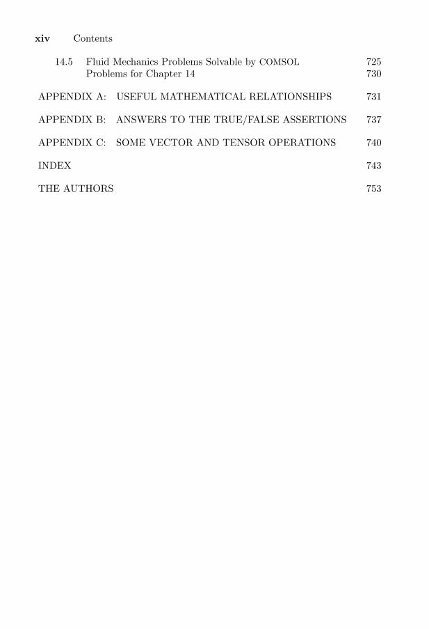
14.5 Fluid Mechanics Problems Solvable by COMSOL 725Problems for Chapter 14 730

APPENDIX A: USEFUL MATHEMATICAL RELATIONSHIPS 731

APPENDIX B: ANSWERS TO THE TRUE/FALSE ASSERTIONS 737

APPENDIX C: SOME VECTOR AND TENSOR OPERATIONS 740

INDEX 743

THE AUTHORS 753

PREFACE

THIS text has evolved from a need for a single volume that embraces a widerange of topics in fluid mechanics. The material consists of two parts—four

chapters on macroscopic or relatively large-scale phenomena, followed by ten chap-ters on microscopic or relatively small-scale phenomena. Throughout, I have triedto keep in mind topics of industrial importance to the chemical engineer. Thescheme is summarized in the following list of chapters.

Part I—Macroscopic Fluid Mechanics

1. Introduction to Fluid Mechanics 3. Fluid Friction in Pipes2. Mass, Energy, and Momentum 4. Flow in Chemical

Balances Engineering Equipment

Part II—Microscopic Fluid Mechanics

5. Differential Equations of Fluid 11. Non-Newtonian FluidsMechanics 12. Microfluidics and

6. Solution of Viscous-Flow Problems Electrokinetic Flow Effects7. Laplace’s Equation, Irrotational 13. An Introduction to

and Porous-Media Flows Computational Fluid8. Boundary-Layer and Other Dynamics and FlowLab

Nearly Unidirectional Flows 14. COMSOL (FEMLAB) Multi-9. Turbulent Flow physics for Solving Fluid

10. Bubble Motion, Two-Phase Flow, Mechanics Problemsand Fluidization

In our experience, an undergraduate fluid mechanics course can be based onPart I plus selected parts of Part II, and a graduate course can be based onmuch of Part II, supplemented perhaps by additional material on topics such asapproximate methods and stability.

Second edition. I have attempted to bring the book up to date by the ma-jor addition of Chapters 12, 13, and 14—one on microfluidics and two on CFD(computational fluid dynamics). The choice of software for the CFD presenteda difficulty; for various reasons, I selected FlowLab and COMSOL Multiphysics,but there was no intention of “promoting” these in favor of other excellent CFDprograms.1 The use of CFD examples in the classroom really makes the subject

1 The software name “FEMLAB” was changed to “COMSOL Multiphysics” in September 2005, the firstrelease under the new name being COMSOL 3.2.

xv

xvi Preface

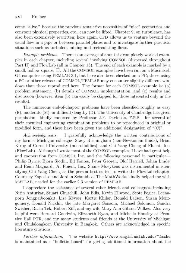
come “alive,” because the previous restrictive necessities of “nice” geometries andconstant physical properties, etc., can now be lifted. Chapter 9, on turbulence, hasalso been extensively rewritten; here again, CFD allows us to venture beyond theusual flow in a pipe or between parallel plates and to investigate further practicalsituations such as turbulent mixing and recirculating flows.

Example problems. There is an average of about six completely worked exam-ples in each chapter, including several involving COMSOL (dispersed throughoutPart II) and FlowLab (all in Chapter 13). The end of each example is marked by asmall, hollow square: . All the COMSOL examples have been run on a MacintoshG4 computer using FEMLAB 3.1, but have also been checked on a PC; those usinga PC or other releases of COMSOL/FEMLAB may encounter slightly different win-dows than those reproduced here. The format for each COMSOL example is: (a)problem statement, (b) details of COMSOL implementation, and (c) results anddiscussion (however, item (b) can easily be skipped for those interested only in theresults).

The numerous end-of-chapter problems have been classified roughly as easy(E), moderate (M), or difficult/lengthy (D). The University of Cambridge has givenpermission—kindly endorsed by Professor J.F. Davidson, F.R.S.—for several oftheir chemical engineering examination problems to be reproduced in original ormodified form, and these have been given the additional designation of “(C)”.

Acknowledgments. I gratefully acknowledge the written contributions ofmy former Michigan colleague Stacy Birmingham (non-Newtonian fluids), BrianKirby of Cornell University (microfluidics), and Chi-Yang Cheng of Fluent, Inc.(FlowLab). Although I wrote most of the COMSOL examples, I have had great helpand cooperation from COMSOL Inc. and the following personnel in particular—Philip Byrne, Bjorn Sjodin, Ed Fontes, Peter Georen, Olof Hernell, Johan Linde,and Remi Magnard. At Fluent, Inc., Shane Moeykens was instrumental in iden-tifying Chi-Yang Cheng as the person best suited to write the FlowLab chapter.Courtney Esposito and Jordan Schmidt of The MathWorks kindly helped me withMATLAB, needed for the earlier 2.3 version of FEMLAB.

I appreciate the assistance of several other friends and colleagues, includingNitin Anturkar, Stuart Churchill, John Ellis, Kevin Ellwood, Scott Fogler, Leena-porn Jongpaiboonkit, Lisa Keyser, Kartic Khilar, Ronald Larson, Susan Mont-gomery, Donald Nicklin, the late Margaret Sansom, Michael Solomon, SandraSwisher, Rasin Tek, Robert Ziff, and my wife Mary Ann Gibson Wilkes. Also veryhelpful were Bernard Goodwin, Elizabeth Ryan, and Michelle Housley at Pren-tice Hall PTR, and my many students and friends at the University of Michiganand Chulalongkorn University in Bangkok. Others are acknowledged in specificliterature citations.

Further information. The website http://www.engin.umich.edu/~fmcheis maintained as a “bulletin board” for giving additional information about the

Preface xvii

book—hints for problem solutions, errata, how to contact the authors, etc.—asproves desirable. My own Internet address is wilkes@umich.edu. The text wascomposed on a Power Macintosh G4 computer using the TEXtures “typesetting”program. Eleven-point type was used for the majority of the text. Most of thefigures were constructed using MacDraw Pro, Excel, and KaleidaGraph.

Professor Terence Fox , to whom this book is dedicated, was a Cambridgeengineering graduate who worked from 1933 to 1937 at Imperial Chemical Indus-tries Ltd., Billingham, Yorkshire. Returning to Cambridge, he taught engineeringfrom 1937 to 1946 before being selected to lead the Department of Chemical En-gineering at the University of Cambridge during its formative years after the endof World War II. As a scholar and a gentleman, Fox was a shy but exceptionallybrilliant person who had great insight into what was important and who quicklybrought the department to a preeminent position. He succeeded in combining anindustrial perspective with intellectual rigor. Fox relinquished the leadership ofthe department in 1959, after he had secured a permanent new building for it(carefully designed in part by himself).

T.R.C. Fox

Fox was instrumental in bringing Peter Danckwerts, Ken-neth Denbigh, John Davidson, and others into the de-partment. He also accepted me in 1956 as a junior fac-ulty member, and I spent four good years in the Cam-bridge University Department of Chemical Engineering.Danckwerts subsequently wrote an appreciation2 of Fox’stalents, saying, with almost complete accuracy: “Fox in-stigated no research and published nothing.” How timeshave changed—today, unless he were known personally,his resume would probably be cast aside and he wouldstand little chance of being hired, let alone of receiv-ing tenure! However, his lectures, meticulously writ-ten handouts, enthusiasm, genius, and friendship werea great inspiration to me, and I have much pleasure in

acknowledging his positive impact on my career.

James O. WilkesAugust 18, 2005

2 P.V. Danckwerts, “Chemical engineering comes to Cambridge,” The Cambridge Review , pp. 53–55, Febru-ary 28, 1983.

This page intentionally left blank

Some Greek Letters

α alpha ν nuβ beta ξ,Ξ xiγ,Γ gamma o omicronδ,Δ delta π,,Π piε, ε epsilon ρ, rhoζ zeta σ, ς,Σ sigmaη eta τ tauθ, ϑ,Θ theta υ,Υ upsilonι iota φ, ϕ,Φ phiκ kappa χ chiλ,Λ lambda ψ,Ψ psiμ mu ω,Ω omega

Chapter 1

INTRODUCTION TO FLUID MECHANICS

1.1 Fluid Mechanics in Chemical Engineering

A knowledge of fluid mechanics is essential for the chemical engineer becausethe majority of chemical-processing operations are conducted either partly or

totally in the fluid phase. Examples of such operations abound in the biochemical,chemical, energy, fermentation, materials, mining, petroleum, pharmaceuticals,polymer, and waste-processing industries.

There are two principal reasons for placing such an emphasis on fluids. First,at typical operating conditions, an enormous number of materials normally existas gases or liquids, or can be transformed into such phases. Second, it is usuallymore efficient and cost-effective to work with fluids in contrast to solids. Evensome operations with solids can be conducted in a quasi-fluidlike manner; exam-ples are the fluidized-bed catalytic refining of hydrocarbons, and the long-distancepipelining of coal particles using water as the agitating and transporting medium.

Although there is inevitably a significant amount of theoretical development,almost all the material in this book has some application to chemical processingand other important practical situations. Throughout, we shall endeavor to presentan understanding of the physical behavior involved; only then is it really possibleto comprehend the accompanying theory and equations.

1.2 General Concepts of a Fluid

We must begin by responding to the question, “What is a fluid?” Broadlyspeaking, a fluid is a substance that will deform continuously when it is subjectedto a tangential or shear force, much as a similar type of force is exerted whena water-skier skims over the surface of a lake or butter is spread on a slice ofbread. The rate at which the fluid deforms continuously depends not only on themagnitude of the applied force but also on a property of the fluid called its viscosityor resistance to deformation and flow. Solids will also deform when sheared, buta position of equilibrium is soon reached in which elastic forces induced by thedeformation of the solid exactly counterbalance the applied shear force, and furtherdeformation ceases.

3

4 Chapter 1—Introduction to Fluid Mechanics

A simple apparatus for shearing a fluid is shown in Fig. 1.1. The fluid iscontained between two concentric cylinders; the outer cylinder is stationary, andthe inner one (of radius R) is rotated steadily with an angular velocity ω. Thisshearing motion of a fluid can continue indefinitely, provided that a source ofenergy—supplied by means of a torque here—is available for rotating the innercylinder. The diagram also shows the resulting velocity profile; note that thevelocity in the direction of rotation varies from the peripheral velocity Rω of theinner cylinder down to zero at the outer stationary cylinder, these representingtypical no-slip conditions at both locations. However, if the intervening spaceis filled with a solid—even one with obvious elasticity, such as rubber—only alimited rotation will be possible before a position of equilibrium is reached, unless,of course, the torque is so high that slip occurs between the rubber and the cylinder.

Fixedcylinder

A A

(b) Plan of section across A-A (not to scale) (a) Side elevation

Fluid

Fluid

Velocity profile

Rotatingcylinder

Rotatingcylinder

ω

Fixedcylinder

R ω

R

Fig. 1.1 Shearing of a fluid.

There are various classes of fluids. Those that behave according to nice and ob-vious simple laws, such as water, oil, and air, are generally called Newtonian fluids.These fluids exhibit constant viscosity but, under typical processing conditions,virtually no elasticity. Fortunately, a very large number of fluids of interest to thechemical engineer exhibit Newtonian behavior, which will be assumed throughoutthe book, except in Chapter 11, which is devoted to the study of non-Newtonianfluids.

A fluid whose viscosity is not constant (but depends, for example, on theintensity to which it is being sheared), or which exhibits significant elasticity, istermed non-Newtonian. For example, several polymeric materials subject to defor-mation can “remember” their recent molecular configurations, and in attemptingto recover their recent states, they will exhibit elasticity in addition to viscosity.Other fluids, such as drilling mud and toothpaste, behave essentially as solids and

1.3—Stresses, Pressure, Velocity, and the Basic Laws 5

will not flow when subject to small shear forces, but will flow readily under theinfluence of high shear forces.

Fluids can also be broadly classified into two main categories—liquids andgases. Liquids are characterized by relatively high densities and viscosities, withmolecules close together; their volumes tend to remain constant, roughly indepen-dent of pressure, temperature, or the size of the vessels containing them. Gases,on the other hand, have relatively low densities and viscosities, with moleculesfar apart; generally, they will rapidly tend to fill the container in which they areplaced. However, these two states—liquid and gaseous—represent but the twoextreme ends of a continuous spectrum of possibilities.

•

••

T

L

G

P

CVapor-pressurecurve

Fig. 1.2 When does a liquid become a gas?

The situation is readily illustrated by considering a fluid that is initially a gasat point G on the pressure/temperature diagram shown in Fig. 1.2. By increasingthe pressure, and perhaps lowering the temperature, the vapor-pressure curve issoon reached and crossed, and the fluid condenses and apparently becomes a liquidat point L. By continuously adjusting the pressure and temperature so that theclockwise path is followed, and circumnavigating the critical point C in the process,the fluid is returned to G, where it is presumably once more a gas. But where doesthe transition from liquid at L to gas at G occur? The answer is at no single point,but rather that the change is a continuous and gradual one, through a wholespectrum of intermediate states.

1.3 Stresses, Pressure, Velocity, and the Basic Laws

Stresses. The concept of a force should be readily apparent. In fluid mechan-ics, a force per unit area, called a stress, is usually found to be a more convenientand versatile quantity than the force itself. Further, when considering a specificsurface, there are two types of stresses that are particularly important.

1. The first type of stress, shown in Fig. 1.3(a), acts perpendicularly to thesurface and is therefore called a normal stress; it will be tensile or compressive,depending on whether it tends to stretch or to compress the fluid on which it acts.The normal stress equals F/A, where F is the normal force and A is the area ofthe surface on which it acts. The dotted outlines show the volume changes caused

6 Chapter 1—Introduction to Fluid Mechanics

by deformation. In fluid mechanics, pressure is usually the most important typeof compressive stress, and will shortly be discussed in more detail.

2. The second type of stress, shown in Fig. 1.3(b), acts tangentially to thesurface; it is called a shear stress τ , and equals F/A, where F is the tangentialforce and A is the area on which it acts. Shear stress is transmitted through afluid by interaction of the molecules with one another. A knowledge of the shearstress is very important when studying the flow of viscous Newtonian fluids. Fora given rate of deformation, measured by the time derivative dγ/dt of the smallangle of deformation γ, the shear stress τ is directly proportional to the viscosityof the fluid (see Fig. 1.3(b)).

F

F

F

F

Area A

Fig. 1.3(a) Tensile and compressive normal stresses F/A, act-ing on a cylinder, causing elongation and shrinkage, respectively.

F

F

Originalposition

Deformedposition

Area Aγ

Fig. 1.3(b) Shear stress τ = F/A, acting on a rectangularparallelepiped, shown in cross section, causing a deformationmeasured by the angle γ (whose magnitude is exaggerated here).

Pressure. In virtually all hydrostatic situations—those involving fluids atrest—the fluid molecules are in a state of compression. For example, for theswimming pool whose cross section is depicted in Fig. 1.4, this compression at atypical point P is caused by the downwards gravitational weight of the water abovepoint P. The degree of compression is measured by a scalar, p—the pressure.

A small inflated spherical balloon pulled down from the surface and tetheredat the bottom by a weight will still retain its spherical shape (apart from a smalldistortion at the point of the tether), but will be diminished in size, as in Fig.1.4(a). It is apparent that there must be forces acting normally inward on the

1.3—Stresses, Pressure, Velocity, and the Basic Laws 7

surface of the balloon, and that these must essentially be uniform for the shape toremain spherical, as in Fig. 1.4(b).

Surface

Balloon

• P

(a) (b)

Water

Water

Balloon

Fig. 1.4 (a) Balloon submerged in a swimming pool; (b) enlargedview of the compressed balloon, with pressure forces acting on it.

Although the pressure p is a scalar, it typically appears in tandem with an areaA (assumed small enough so that the pressure is uniform over it). By definitionof pressure, the surface experiences a normal compressive force F = pA. Thus,pressure has units of a force per unit area—the same as a stress.

The value of the pressure at a point is independent of the orientation of anyarea associated with it, as can be deduced with reference to a differentially smallwedge-shaped element of the fluid, shown in Fig. 1.5.

θ

pA

pB

pC

z

y

x

π2

− θ

dA

dB

dCdA

dB

dC

Fig. 1.5 Equilibrium of a wedge of fluid.

Due to the pressure there are three forces, pAdA, pBdB, and pCdC, that acton the three rectangular faces of areas dA, dB, and dC. Since the wedge is notmoving, equate the two forces acting on it in the horizontal or x direction, notingthat pAdA must be resolved through an angle (π/2 − θ) by multiplying it bycos(π/2 − θ) = sin θ:

pAdA sin θ = pCdC. (1.1)

The vertical force pBdB acting on the bottom surface is omitted from Eqn. (1.1)because it has no component in the x direction. The horizontal pressure forces

8 Chapter 1—Introduction to Fluid Mechanics

acting in the y direction on the two triangular faces of the wedge are also omit-ted, since again these forces have no effect in the x direction. From geometricalconsiderations, areas dA and dC are related by:

dC = dA sin θ. (1.2)

These last two equations yield:pA = pC , (1.3)

verifying that the pressure is independent of the orientation of the surface beingconsidered. A force balance in the z direction leads to a similar result, pA = pB.1

For moving fluids, the normal stresses include both a pressure and extrastresses caused by the motion of the fluid, as discussed in detail in Section 5.6.

The amount by which a certain pressure exceeds that of the atmosphere istermed the gauge pressure, the reason being that many common pressure gaugesare really differential instruments, reading the difference between a required pres-sure and that of the surrounding atmosphere. Absolute pressure equals the gaugepressure plus the atmospheric pressure.

Velocity. Many problems in fluid mechanics deal with the velocity of thefluid at a point, equal to the rate of change of the position of a fluid particlewith time, thus having both a magnitude and a direction. In some situations,particularly those treated from the macroscopic viewpoint, as in Chapters 2, 3,and 4, it sometimes suffices to ignore variations of the velocity with position.In other cases—particularly those treated from the microscopic viewpoint, as inChapter 6 and later—it is invariably essential to consider variations of velocitywith position.

u A u A

(a) (b)

Fig. 1.6 Fluid passing through an area A:(a) Uniform velocity, (b) varying velocity.

Velocity is not only important in its own right, but leads immediately to threefluxes or flow rates. Specifically, if u denotes a uniform velocity (not varying withposition):

1 Actually, a force balance in the z direction demands that the gravitational weight of the wedge be considered,which is proportional to the volume of the wedge. However, the pressure forces are proportional to theareas of the faces. It can readily be shown that the volume-to-area effect becomes vanishingly small as thewedge becomes infinitesimally small, so that the gravitational weight is inconsequential.

1.3—Stresses, Pressure, Velocity, and the Basic Laws 9

1. If the fluid passes through a plane of area A normal to the direction of thevelocity, as shown in Fig. 1.6, the corresponding volumetric flow rate of fluidthrough the plane is Q = uA.

2. The corresponding mass flow rate is m = ρQ = ρuA, where ρ is the (constant)fluid density. The alternative notation with an overdot, m, is also used.

3. When velocity is multiplied by mass it gives momentum, a quantity of primeimportance in fluid mechanics. The corresponding momentum flow rate pass-ing through the area A is M = mu = ρu2A.

If u and/or ρ should vary with position, as in Fig. 1.6(b), the corresponding ex-pressions will be seen later to involve integrals over the area A: Q =

∫Au dA, m =∫

Aρu dA, M =

∫Aρu2 dA.

Basic laws. In principle, the laws of fluid mechanics can be stated simply,and—in the absence of relativistic effects—amount to conservation of mass, energy,and momentum. When applying these laws, the procedure is first to identifya system, its boundary, and its surroundings; and second, to identify how thesystem interacts with its surroundings. Refer to Fig. 1.7 and let the quantity Xrepresent either mass, energy, or momentum. Also recognize that X may be addedfrom the surroundings and transported into the system by an amount Xin acrossthe boundary, and may likewise be removed or transported out of the system tothe surroundings by an amount Xout.

Surroundings

X out

X in

Xdestroyed

Xcreated

System

Boundary

Fig. 1.7 A system and transports to and from it.

The general conservation law gives the increase ΔXsystem in the X-content ofthe system as:

Xin −Xout = ΔXsystem. (1.4a)

Although this basic law may appear intuitively obvious, it applies only to avery restricted selection of properties X. For example, it is not generally true if Xis another extensive property such as volume, and is quite meaningless if X is anintensive property such as pressure or temperature.

In certain cases, where X i is the mass of a definite chemical species i , we mayalso have an amount of creation X i

created or destruction X idestroyed due to chemical

reaction, in which case the general law becomes:

X iin −X i

out + X icreated −X i

destroyed = ΔX isystem. (1.4b)

10 Chapter 1—Introduction to Fluid Mechanics

The conservation law will be discussed further in Section 2.1, and is of such fun-damental importance that in various guises it will find numerous applicationsthroughout all of this text.

To solve a physical problem, the following information concerning the fluid isalso usually needed:1. The physical properties of the fluid involved, as discussed in Section 1.4.2. For situations involving fluid flow , a constitutive equation for the fluid, which

relates the various stresses to the flow pattern.

1.4 Physical Properties—Density, Viscosity, and Surface Tension

There are three physical properties of fluids that are particularly important:density, viscosity, and surface tension. Each of these will be defined and viewedbriefly in terms of molecular concepts, and their dimensions will be examined interms of mass, length, and time (M, L, and T). The physical properties dependprimarily on the particular fluid. For liquids, viscosity also depends strongly onthe temperature; for gases, viscosity is approximately proportional to the squareroot of the absolute temperature. The density of gases depends almost directlyon the absolute pressure; for most other cases, the effect of pressure on physicalproperties can be disregarded.

Typical processes often run almost isothermally, and in these cases the effectof temperature can be ignored. Except in certain special cases, such as the flow ofa compressible gas (in which the density is not constant) or a liquid under a veryhigh shear rate (in which viscous dissipation can cause significant internal heating),or situations involving exothermic or endothermic reactions, we shall ignore anyvariation of physical properties with pressure and temperature.

Densities of liquids. Density depends on the mass of an individual moleculeand the number of such molecules that occupy a unit of volume. For liquids,density depends primarily on the particular liquid and, to a much smaller extent,on its temperature. Representative densities of liquids are given in Table 1.1.2

(See Eqns. (1.9)–(1.11) for an explanation of the specific gravity and coefficient ofthermal expansion columns.) The accuracy of the values given in Tables 1.1–1.6is adequate for the calculations needed in this text. However, if highly accuratevalues are needed, particularly at extreme conditions, then specialized informationshould be sought elsewhere.

Density. The density ρ of a fluid is defined as its mass per unit volume, andindicates its inertia or resistance to an accelerating force. Thus:

ρ =mass

volume[=]

ML3

, (1.5)

2 The values given in Tables 1.1, 1.3, 1.4, 1.5, and 1.6 are based on information given in J.H. Perry, ed.,Chemical Engineers’ Handbook, 3rd ed., McGraw-Hill, New York, 1950.

1.4—Physical Properties—Density, Viscosity, and Surface Tension 11

in which the notation “[=]” is consistently used to indicate the dimensions of aquantity.3 It is usually understood in Eqn. (1.5) that the volume is chosen so thatit is neither so small that it has no chance of containing a representative selectionof molecules nor so large that (in the case of gases) changes of pressure causesignificant changes of density throughout the volume. A medium characterizedby a density is called a continuum, and follows the classical laws of mechanics—including Newton’s law of motion, as described in this book.

Table 1.1 Specific Gravities, Densities, andThermal Expansion Coefficients of Liquids at 20 ◦C

Liquid Sp. Gr. Density, ρ αs kg/m3 lbm/ft3 ◦C−1

Acetone 0.792 792 49.4 0.00149Benzene 0.879 879 54.9 0.00124Crude oil, 35◦API 0.851 851 53.1 0.00074Ethanol 0.789 789 49.3 0.00112Glycerol 1.26 (50 ◦C) 1,260 78.7 —Kerosene 0.819 819 51.1 0.00093Mercury 13.55 13,550 845.9 0.000182Methanol 0.792 792 49.4 0.00120n-Octane 0.703 703 43.9 —n-Pentane 0.630 630 39.3 0.00161Water 0.998 998 62.3 0.000207

Degrees A.P.I. (American Petroleum Institute) are related to specific gravity sby the formula:

◦A.P.I. =141.5s

− 131.5. (1.6)

Note that for water, ◦A.P.I. = 10, with correspondingly higher values for liquidsthat are less dense. Thus, for the crude oil listed in Table 1.1, Eqn. (1.6) indeedgives 141.5/0.851 − 131.5 .= 35 ◦A.P.I.

Densities of gases. For ideal gases, pV = nRT , where p is the absolutepressure, V is the volume of the gas, n is the number of moles (abbreviated as “mol”when used as a unit), R is the gas constant, and T is the absolute temperature. IfMw is the molecular weight of the gas, it follows that:

ρ =nMw

V=

Mwp

RT. (1.7)

3 An early appearance of the notation “[=]” is in R.B. Bird, W.E. Stewart, and E.N. Lightfoot, TransportPhenomena, Wiley, New York, 1960.

12 Chapter 1—Introduction to Fluid Mechanics

Thus, the density of an ideal gas depends on the molecular weight, absolute pres-sure, and absolute temperature. Values of the gas constant R are given in Table1.2 for various systems of units. Note that degrees Kelvin, formerly representedby “ ◦K,” is now more simply denoted as “K.”

Table 1.2 Values of the Gas Constant, R

Value Units

8.314 J/g-mol K0.08314 liter bar/g-mol K0.08206 liter atm/g-mol K1.987 cal/g-mol K10.73 psia ft3/lb-mol ◦R0.7302 ft3 atm/lb-mol ◦R1,545 ft lbf/lb-mol ◦R

For a nonideal gas, the compressibility factor Z (a function of p and T ) isintroduced into the denominator of Eqn. (1.7), giving:

ρ =nMw

V=

Mwp

ZRT. (1.8)

Thus, the extent to which Z deviates from unity gives a measure of the nonidealityof the gas.

The isothermal compressibility of a gas is defined as:

β = − 1V

(∂V

∂p

)T

,

and equals—at constant temperature—the fractional decrease in volume causedby a unit increase in the pressure. For an ideal gas, β = 1/p, the reciprocal of theabsolute pressure.

The coefficient of thermal expansion α of a material is its isobaric (constantpressure) fractional increase in volume per unit rise in temperature:

α =1V

(∂V

∂T

)p

. (1.9)

Since, for a given mass, density is inversely proportional to volume, it follows thatfor moderate temperature ranges (over which α is essentially constant) the densityof most liquids is approximately a linear function of temperature:

ρ.= ρ0[1 − α(T − T0)], (1.10)

1.4—Physical Properties—Density, Viscosity, and Surface Tension 13

where ρ0 is the density at a reference temperature T0. For an ideal gas, α = 1/T ,the reciprocal of the absolute temperature.

The specific gravity s of a fluid is the ratio of the density ρ to the density ρSC

of a reference fluid at some standard condition:

s =ρ

ρSC

. (1.11)

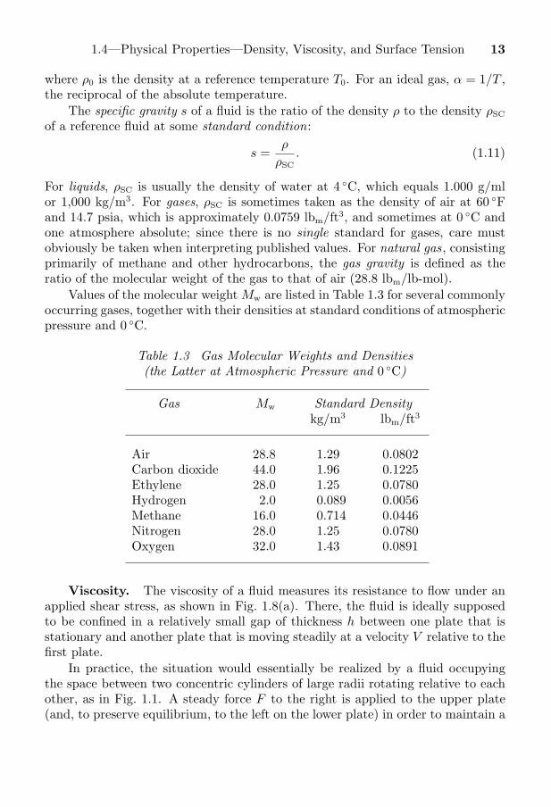
For liquids, ρSC is usually the density of water at 4 ◦C, which equals 1.000 g/mlor 1,000 kg/m3. For gases, ρSC is sometimes taken as the density of air at 60 ◦Fand 14.7 psia, which is approximately 0.0759 lbm/ft3, and sometimes at 0 ◦C andone atmosphere absolute; since there is no single standard for gases, care mustobviously be taken when interpreting published values. For natural gas, consistingprimarily of methane and other hydrocarbons, the gas gravity is defined as theratio of the molecular weight of the gas to that of air (28.8 lbm/lb-mol).

Values of the molecular weight Mw are listed in Table 1.3 for several commonlyoccurring gases, together with their densities at standard conditions of atmosphericpressure and 0 ◦C.

Table 1.3 Gas Molecular Weights and Densities(the Latter at Atmospheric Pressure and 0 ◦C)

Gas Mw Standard Densitykg/m3 lbm/ft3

Air 28.8 1.29 0.0802Carbon dioxide 44.0 1.96 0.1225Ethylene 28.0 1.25 0.0780Hydrogen 2.0 0.089 0.0056Methane 16.0 0.714 0.0446Nitrogen 28.0 1.25 0.0780Oxygen 32.0 1.43 0.0891

Viscosity. The viscosity of a fluid measures its resistance to flow under anapplied shear stress, as shown in Fig. 1.8(a). There, the fluid is ideally supposedto be confined in a relatively small gap of thickness h between one plate that isstationary and another plate that is moving steadily at a velocity V relative to thefirst plate.

In practice, the situation would essentially be realized by a fluid occupyingthe space between two concentric cylinders of large radii rotating relative to eachother, as in Fig. 1.1. A steady force F to the right is applied to the upper plate(and, to preserve equilibrium, to the left on the lower plate) in order to maintain a

14 Chapter 1—Introduction to Fluid Mechanics

constant motion and to overcome the viscous friction caused by layers of moleculessliding over one another.

h

y

Fixed plate

(a) (b)

Velocity V

u = yh

V

Moving plate

Fixed plate

Fluid

Force F

Force F

Velocity profile

Moving plate u = V

Fig. 1.8 (a) Fluid in shear between parallelplates; (b) the ensuing linear velocity profile.

Under these circumstances, the velocity u of the fluid to the right is foundexperimentally to vary linearly from zero at the lower plate (y = 0) to V itselfat the upper plate, as in Fig. 1.8(b), corresponding to no-slip conditions at eachplate. At any intermediate distance y from the lower plate, the velocity is simply:

u =y

hV. (1.12)

Recall that the shear stress τ is the tangential applied force F per unit area:

τ =F

A, (1.13)

in which A is the area of each plate. Experimentally, for a large class of materials,called Newtonian fluids, the shear stress is directly proportional to the velocitygradient:

τ = μdu

dy= μ

V

h. (1.14)

The proportionality constant μ is called the viscosity of the fluid; its dimensionscan be found by substituting those for F (ML/T2), A (L2), and du/dy (T−1),giving:

μ [=]MLT

. (1.15)

Representative units for viscosity are g/cm s (also known as poise, designatedby P), kg/m s, and lbm/ft hr. The centipoise (cP), one hundredth of a poise,is also a convenient unit, since the viscosity of water at room temperature isapproximately 0.01 P or 1.0 cP. Table 1.11 gives viscosity conversion factors.

The viscosity of a fluid may be determined by observing the pressure drop whenit flows at a known rate in a tube, as analyzed in Section 3.2. More sophisticated

1.4—Physical Properties—Density, Viscosity, and Surface Tension 15

methods for determining the rheological or flow properties of fluids—includingviscosity—are also discussed in Chapter 11; such methods often involve containingthe fluid in a small gap between two surfaces, moving one of the surfaces, andmeasuring the force needed to maintain the other surface stationary.

Table 1.4 Viscosity Parameters for Liquids

Liquid a b a b(T in K) (T in ◦R)

Acetone 14.64 −2.77 16.29 −2.77Benzene 21.99 −3.95 24.34 −3.95Crude oil, 35◦ API 53.73 −9.01 59.09 −9.01Ethanol 31.63 −5.53 34.93 −5.53Glycerol 106.76 −17.60 117.22 −17.60Kerosene 33.41 −5.72 36.82 −5.72Methanol 22.18 −3.99 24.56 −3.99Octane 17.86 −3.25 19.80 −3.25Pentane 13.46 −2.62 15.02 −2.62Water 29.76 −5.24 32.88 −5.24

The kinematic viscosity ν is the ratio of the viscosity to the density:

ν =μ

ρ, (1.16)

and is important in cases in which significant viscous and gravitational forcescoexist. The reader can check that the dimensions of ν are L2/T, which areidentical to those for the diffusion coefficient D in mass transfer and for the thermaldiffusivity α = k/ρcp in heat transfer. There is a definite analogy among the threequantities—indeed, as seen later, the value of the kinematic viscosity governs therate of “diffusion” of momentum in the laminar and turbulent flow of fluids.

Viscosities of liquids. The viscosities μ of liquids generally vary approximatelywith absolute temperature T according to:

lnμ.= a + b lnT or μ

.= ea+b ln T , (1.17)

and—to a good approximation—are independent of pressure. Assuming that μ ismeasured in centipoise and that T is either in degrees Kelvin or Rankine, appro-priate parameters a and b are given in Table 1.4 for several representative liquids.The resulting values for viscosity are approximate, suitable for a first design only.

16 Chapter 1—Introduction to Fluid Mechanics

Viscosities of gases. The viscosity μ of many gases is approximated by theformula:

μ.= μ0

(T

T0

)n

, (1.18)

in which T is the absolute temperature (Kelvin or Rankine), μ0 is the viscosity atan absolute reference temperature T0, and n is an empirical exponent that bestfits the experimental data. The values of the parameters μ0 and n for atmosphericpressure are given in Table 1.5; recall that to a first approximation, the viscosityof a gas is independent of pressure. The values μ0 are given in centipoise andcorrespond to a reference temperature of T0

.= 273 K .= 492 ◦R.

Table 1.5 Viscosity Parameters for Gases

Gas μ0, cP n

Air 0.0171 0.768Carbon dioxide 0.0137 0.935Ethylene 0.0096 0.812Hydrogen 0.0084 0.695Methane 0.0120 0.873Nitrogen 0.0166 0.756Oxygen 0.0187 0.814

Surface tension.4 Surface tension is the tendency of the surface of a liquid tobehave like a stretched elastic membrane. There is a natural tendency for liquidsto minimize their surface area. The obvious case is that of a liquid droplet on ahorizontal surface that is not wetted by the liquid—mercury on glass, or water ona surface that also has a thin oil film on it. For small droplets, such as those onthe left of Fig. 1.9, the droplet adopts a shape that is almost perfectly spherical,because in this configuration there is the least surface area for a given volume.

Fig. 1.9 The larger droplets are flatter because grav-ity is becoming more important than surface tension.

4 We recommend that this subsection be omitted at a first reading, because the concept of surface tension issomewhat involved and is relevant only to a small part of this book.

1.4—Physical Properties—Density, Viscosity, and Surface Tension 17

For larger droplets, the shape becomes somewhat flatter because of the increasinglyimportant gravitational effect, which is roughly proportional to a3, where a is theapproximate droplet radius, whereas the surface area is proportional only to a2.Thus, the ratio of gravitational to surface tension effects depends roughly on thevalue of a3/a2 = a, and is therefore increasingly important for the larger droplets,as shown to the right in Fig. 1.9. Overall, the situation is very similar to that ofa water-filled balloon, in which the water accounts for the gravitational effect andthe balloon acts like the surface tension.

A fundamental property is the surface energy , which is defined with referenceto Fig. 1.10(a). A molecule I, situated in the interior of the liquid, is attractedequally in all directions by its neighbors. However, a molecule S, situated inthe surface, experiences a net attractive force into the bulk of the liquid. (Thevapor above the surface, being comparatively rarefied, exerts a negligible force onmolecule S.) Therefore, work has to be done against such a force in bringing aninterior molecule to the surface. Hence, an energy σ, called the surface energy, canbe attributed to a unit area of the surface.

Molecule S Freesurface

TT

L

W

(a) (b)

Molecule I

Liquid Newlycreatedsurface

Fig. 1.10 (a) Molecules in the interior and surface of a liquid; (b) newlycreated surface caused by moving the tension T through a distance L.

An equivalent viewpoint is to consider the surface tension T existing per unitdistance of a line drawn in the surface, as shown in Fig. 1.10(b). Suppose that sucha tension has moved a distance L, thereby creating an area WL of fresh surface.The work done is the product of the force, TW , and the distance L through whichit moves, namely TWL, and this must equal the newly acquired surface energyσWL. Therefore, T = σ; both quantities have units of force per unit distance,such as N/m, which is equivalent to energy per unit area, such as J/m2.

We next find the amount p1−p2 by which the pressure p1 inside a liquid dropletof radius r, shown in Fig. 1.11(a), exceeds the pressure p2 of the surrounding vapor.Fig. 1.11(b) illustrates the equilibrium of the upper hemisphere of the droplet,which is also surrounded by an imaginary cylindrical “control surface” ABCD,on which forces in the vertical direction will soon be equated. Observe that the

18 Chapter 1—Introduction to Fluid Mechanics

internal pressure p1 is trying to blow apart the two hemispheres (the lower one isnot shown), whereas the surface tension σ is trying to pull them together.

(a) Liquid droplet

A B

C

Vapor

Liquid

r

O

σ

(b) Forces in equilibrium

p2

p1

D • r

σ

O

Liquid

Vaporp2

p1

Fig. 1.11 Pressure change across a curved surface.

In more detail, there are two different types of forces to be considered:1. That due to the pressure difference between the pressure inside the droplet

and the vapor outside, each acting on an area πr2 (that of the circles CD andAB):

(p1 − p2)πr2. (1.19)2. That due to surface tension, which acts on the circumference of length 2πr:

2πrσ. (1.20)At equilibrium, these two forces are equated, giving:

Δp = p1 − p2 =2σr. (1.21)

That is, there is a higher pressure on the concave or droplet side of the interface.What would the pressure change be for a bubble instead of a droplet? Why?

More generally, if an interface has principal radii of curvature r1 and r2, theincrease in pressure can be shown to be:

p1 − p2 = σ

(1r1

+1r2

). (1.22)

For a sphere of radius r, as in Fig. 1.11, both radii are equal, so that r1 = r2 = r,and p1 − p2 = 2σ/r. Problem 1.31 involves a situation in which r1 �= r2. The radiir1 and r2 will have the same sign if the corresponding centers of curvature are onthe same side of the interface; if not, they will be of opposite sign. Appendix Acontains further information about the curvature of a surface.

1.4—Physical Properties—Density, Viscosity, and Surface Tension 19

(c)

Film with two sides

Force F

Ring ofperimeter

P

Pσ Pσ

Liquid

(b)

D

Capillary tube

Droplet

Liquid

σ σ

(a)

h

••

•

1

2

3

2a

θContactangle,

Meniscus

Capillary tube

Liquid

θ

r

a

Circle of which the interface is a part

Tubewall

•4

θ

Fig. 1.12 Methods for measuring surface tension.

A brief description of simple experiments for measuring the surface tension σof a liquid, shown in Fig. 1.12, now follows:

(a) In the capillary-rise method, a narrow tube of internal radius a is dippedvertically into a pool of liquid, which then rises to a height h inside the tube; if thecontact angle (the angle between the free surface and the wall) is θ, the meniscuswill be approximated by part of the surface of a sphere; from the geometry shownin the enlargement on the right-hand side of Fig. 1.12(a) the radius of the sphereis seen to be r = a/ cos θ. Since the surface is now concave on the air side, thereverse of Eqn. (1.21) occurs, and p2 = p1 − 2σ/r, so that p2 is below atmosphericpressure p1. Now follow the path 1–2–3–4, and observe that p4 = p3 because points

20 Chapter 1—Introduction to Fluid Mechanics

3 and 4 are at the same elevation in the same liquid. Thus, the pressure at point 4is:

p4 = p1 − 2σr

+ ρgh.

However, p4 = p1 since both of these are at atmospheric pressure. Hence, thesurface tension is given by the relation:

σ =12ρghr =

ρgha

2 cos θ. (1.23)

In many cases—for complete wetting of the surface—θ is essentially zero andcos θ = 1. However, for liquids such as mercury in glass, there may be a com-plete non-wetting of the surface, in which case θ = π, so that cos θ = −1; theresult is that the liquid level in the capillary is then depressed below that in thesurrounding pool.

(b) In the drop-weight method, a liquid droplet is allowed to form very slowlyat the tip of a capillary tube of outer diameter D. The droplet will eventually growto a size where its weight just overcomes the surface-tension force πDσ holding itup. At this stage, it will detach from the tube, and its weight w = Mg can bedetermined by catching it in a small pan and weighing it. By equating the twoforces, the surface tension is then calculated from:

σ =w

πD. (1.24)

(c) In the ring tensiometer, a thin wire ring, suspended from the arm of asensitive balance, is dipped into the liquid and gently raised, so that it brings athin liquid film up with it. The force F needed to support the film is measuredby the balance. The downward force exerted on a unit length of the ring by oneside of the film is the surface tension; since there are two sides to the film, thetotal force is 2Pσ, where P is the circumference of the ring. The surface tensionis therefore determined as:

σ =F

2P. (1.25)

In common with most experimental techniques, all three methods describedabove require slight modifications to the results expressed in Eqns. (1.23)–(1.25)because of imperfections in the simple theories.

Surface tension generally appears only in situations involving either free sur-faces (liquid/gas or liquid/solid boundaries) or interfaces (liquid/liquid bound-aries); in the latter case, it is usually called the interfacial tension.

Representative values for the surface tensions of liquids at 20 ◦C, in contacteither with air or their vapor (there is usually little difference between the two),are given in Table 1.6.5

5 The values for surface tension have been obtained from the CRC Handbook of Chemistry and Physics,48th ed., The Chemical Rubber Co., Cleveland, OH, 1967.

1.5—Units and Systems of Units 21

Table 1.6 Surface Tensions

Liquid σdynes/cm

Acetone 23.70Benzene 28.85Ethanol 22.75Glycerol 63.40Mercury 435.5Methanol 22.61n-Octane 21.80Water 72.75

1.5 Units and Systems of Units

Mass, weight, and force. The mass M of an object is a measure of theamount of matter it contains and will be constant, since it depends on the numberof constituent molecules and their masses. On the other hand, the weight w of theobject is the gravitational force on it, and is equal to Mg, where g is the localgravitational acceleration. Mostly, we shall be discussing phenomena occurring atthe surface of the earth, where g is approximately 32.174 ft/s2 = 9.807 m/s2 =980.7 cm/s2. For much of this book, these values are simply taken as 32.2, 9.81,and 981, respectively.

Table 1.7 Representative Units of Force

System Units of Force Customary Name

SI kg m/s2 newtonCGS g cm/s2 dyneFPS lbm ft/s2 poundal

Newton’s second law of motion states that a force F applied to a mass M willgive it an acceleration a:

F = Ma, (1.26)

from which is apparent that force has dimensions ML/T2. Table 1.7 gives thecorresponding units of force in the SI (meter/kilogram/second), CGS (centime-ter/gram/second), and FPS (foot/pound/second) systems.

22 Chapter 1—Introduction to Fluid Mechanics

The poundal is now an archaic unit, hardly ever used. Instead, the pound force,lbf , is much more common in the English system; it is defined as the gravitationalforce on 1 lbm, which, if left to fall freely, will do so with an acceleration of 32.2ft/s2. Hence:

1 lbf = 32.2 lbm

fts2

= 32.2 poundals. (1.27)

Table 1.8 SI Units

Physical Name of Symbol DefinitionQuantity Unit for Unit of Unit

Basic UnitsLength meter m –Mass kilogram kg –Time second s –Temperature degree

Kelvin K –

Supplementary UnitPlane angle radian rad —

Derived UnitsAcceleration m/s2

Angularvelocity rad/s

Density kg/m3

Energy joule J kg m2/s2

Force newton N kg m/s2

Kinematicviscosity m2/s

Power watt W kg m2/s3 (J/s)Pressure pascal Pa kg/m s2 (N/m2)Velocity m/sViscosity kg/m s

When using lbf in the ft, lbm, s (FPS) system, the following conversion factor,commonly called “gc,” will almost invariably be needed:

gc = 32.2lbm ft/s2

lbf

= 32.2lbm ftlbf s2

. (1.28)

1.5—Units and Systems of Units 23

Some writers incorporate gc into their equations, but this approach may be con-fusing since it virtually implies that one particular set of units is being used, andhence tends to rob the equations of their generality. Why not, for example, alsoincorporate the conversion factor of 144 in2/ft2 into equations where pressure isexpressed in lbf/in2? We prefer to omit all conversion factors in equations, andintroduce them only as needed in evaluating expressions numerically. If the readeris in any doubt, units should always be checked when performing calculations.

SI Units. The most systematically developed and universally accepted setof units occurs in the SI units or Systeme International d’Unites6; the subset wemainly need is shown in Table 1.8.

The basic units are again the meter, kilogram, and second (m, kg, and s); fromthese, certain derived units can also be obtained. Force (kg m/s2) has already beendiscussed; energy is the product of force and length; power amounts to energy perunit time; surface tension is energy per unit area or force per unit length, and soon. Some of the units have names, and these, together with their abbreviations,are also given in Table 1.8.

Table 1.9 Auxiliary Units Allowed in Conjunction with SI Units

Physical Name of Symbol DefinitionQuantity Unit for Unit of Unit

Area hectare ha 104 m2

Kinematic viscosity stokes St 10−4 m2/sLength micron μm 10−6 mMass tonne t 103 kg = Mg

gram g 10−3 kg = gPressure bar bar 105 N/m2

Viscosity poise P 10−1 kg/m sVolume liter l 10−3 m3

Tradition dies hard, and certain other “metric” units are so well establishedthat they may be used as auxiliary units; these are shown in Table 1.9. The gramis the classic example. Note that the basic SI unit of mass (kg) is even representedin terms of the gram, and has not yet been given a name of its own!

Table 1.10 shows some of the acceptable prefixes that can be used for accom-modating both small and large quantities. For example, to avoid an excessivenumber of decimal places, 0.000001 s is normally better expressed as 1 μs (onemicrosecond). Note also, for example, that 1 μkg should be written as 1 mg—oneprefix being better than two.

6 For an excellent discussion, on which Tables 1.8 and 1.9 are based, see Metrication in Scientific Journals,published by The Royal Society, London, 1968.

24 Chapter 1—Introduction to Fluid Mechanics

Table 1.10 Prefixes for Fractions and Multiples

Factor Name Symbol Factor Name Symbol

10−12 pico p 103 kilo k10−9 nano n 106 mega M10−6 micro μ 109 giga G10−3 milli m 1012 tera T

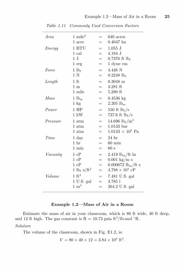
Some of the more frequently used conversion factors are given in Table 1.11.

Example 1.1—Units Conversion

Part 1. Express 65 mph in (a) ft/s, and (b) m/s.

Solution

The solution is obtained by employing conversion factors taken from Table1.11:

(a) 65milehr × 1

3,600hrs × 5,280

ftmile = 95.33

fts .

(b) 95.33fts × 0.3048

mft = 29.06

ms .

Part 2. The density of 35 ◦API crude oil is 53.1 lbm/ft3 at 68 ◦F and itsviscosity is 32.8 lbm/ft hr. What are its density, viscosity, and kinematic viscosityin SI units?

Solution

ρ = 53.1lbm

ft3× 0.4536

kglbm

× 10.30483

ft3

m3 = 851kgm3 .

μ = 32.8lbm

ft hr × 12.419

centipoiselbm/ft hr × 0.01

poisecentipoise = 0.136 poise.

Or, converting to SI units, noting that P is the symbol for poise, and evaluating ν:

μ = 0.136 P × 0.1kg/m s

P = 0.0136kgm s .

ν =μ

ρ=

0.0136 kg/m s851 kg/m3 = 1.60 × 10−5

m2

s (= 0.160 St).

Example 1.2—Mass of Air in a Room 25

Table 1.11 Commonly Used Conversion Factors

Area 1 mile2 = 640 acres1 acre = 0.4047 ha

Energy 1 BTU = 1,055 J1 cal = 4.184 J1 J = 0.7376 ft lbf

1 erg = 1 dyne cmForce 1 lbf = 4.448 N

1 N = 0.2248 lbf

Length 1 ft = 0.3048 m1 m = 3.281 ft1 mile = 5,280 ft

Mass 1 lbm = 0.4536 kg1 kg = 2.205 lbm

Power 1 HP = 550 ft lbf/s1 kW = 737.6 ft lbf/s

Pressure 1 atm = 14.696 lbf/in2

1 atm = 1.0133 bar1 atm = 1.0133 × 105 Pa

Time 1 day = 24 hr1 hr = 60 min1 min = 60 s

Viscosity 1 cP = 2.419 lbm/ft hr1 cP = 0.001 kg/m s1 cP = 0.000672 lbm/ft s1 lbf s/ft2 = 4.788 × 104 cP

Volume 1 ft3 = 7.481 U.S. gal1 U.S. gal = 3.785 l1 m3 = 264.2 U.S. gal

Example 1.2—Mass of Air in a Room

Estimate the mass of air in your classroom, which is 80 ft wide, 40 ft deep,and 12 ft high. The gas constant is R = 10.73 psia ft3/lb-mol ◦R.

SolutionThe volume of the classroom, shown in Fig. E1.2, is:

V = 80 × 40 × 12 = 3.84 × 104 ft3.

26 Chapter 1—Introduction to Fluid Mechanics

80 ft40 ft

12 ft

Fig. E1.2 Assumed dimensions of classroom.

If the air is approximately 20% oxygen and 80% nitrogen, its mean molecularweight is Mw = 0.8×28+0.2×32 = 28.8 lbm/lb-mol. From the gas law, assumingan absolute pressure of p = 14.7 psia and a temperature of 70 ◦F = 530 ◦R, thedensity is:

ρ =Mwp

RT=

28.8 (lbm/lb mol) × 14.7 (psia)

10.73 (psia ft3/lb mol ◦R) × 530 (◦R)= 0.0744 lbm/ft

3.

Hence, the mass of air is:

M = ρV = 0.0744 (lbm/ft3) × 3.84 × 104 (ft3) = 2,860 lbm.

For the rest of the book, manipulation of units will often be less detailed; thereader should always check if there is any doubt.

1.6 Hydrostatics

Variation of pressure with elevation. Here, we investigate how the pres-sure in a stationary fluid varies with elevation z. The result is useful because it cananswer questions such as “What is the pressure at the summit of Mt. Annapurna?”or “What forces are exerted on the walls of an oil storage tank?” Consider a hypo-thetical differential cylindrical element of fluid of cross-sectional area A, height dz,and volume Adz, which is also surrounded by the same fluid, as shown in Fig. 1.13.Its weight, being the downwards gravitational force on its mass, is dW = ρAdz g.Two completely equivalent approaches will be presented:

Method 1. Let p denote the pressure at the base of the cylinder; since pchanges at a rate dp/dz with elevation, the pressure is found either from Taylor’sexpansion or the definition of a derivative to be p + (dp/dz)dz at the top of thecylinder.7 (Note that we do not anticipate a reduction of pressure with elevationhere; hence, the plus sign is used. If, indeed—as proves to be the case—pressurefalls with increasing elevation, then the subsequent development will tell us that

7 Further details of this fundamental statement can be found in Appendix A and must be fully understood,because similar assertions appear repeatedly throughout the book.

1.6—Hydrostatics 27

dp/dz is negative.) Hence, the fluid exerts an upward force of pA on the base ofthe cylinder, and a downward force of [p+ (dp/dz)dz]A on the top of the cylinder.

Next, apply Newton’s second law of motion by equating the net upward forceto the mass times the acceleration—which is zero, since the cylinder is stationary:

pA−(p +

dp

dzdz

)A︸ ︷︷ ︸

Net pressure force

− ρAdz g︸ ︷︷ ︸Weight

= (ρAdz)︸ ︷︷ ︸Mass

×0 = 0. (1.29)

Cancellation of pA and division by Adz leads to the following differential equation,which governs the rate of change of pressure with elevation:

dp

dz= −ρg. (1.30)

Area A

= pz+dzp + dpdz

dz

z = 0

p = pz

dWdz

z

Fig. 1.13 Forces acting on a cylinder of fluid.

Method 2. Let pz and pz+dz denote the pressures at the base and top of thecylinder, where the elevations are z and z+dz, respectively. Hence, the fluid exertsan upward force of pzA on the base of the cylinder, and a downward force of pz+dzAon the top of the cylinder. Application of Newton’s second law of motion gives:

pzA− pz+dzA︸ ︷︷ ︸Net pressure force

− ρAdz g︸ ︷︷ ︸Weight

= (ρAdz)︸ ︷︷ ︸Mass

×0 = 0. (1.31)

Isolation of the two pressure terms on the left-hand side and division by Adz gives:pz+dz − pz

dz= −ρg. (1.32)

As dz tends to zero, the left-hand side of Eqn. (1.32) becomes the derivative dp/dz,leading to the same result as previously:

dp

dz= −ρg. (1.30)

The same conclusion can also be obtained by considering a cylinder of finite heightΔz and then letting Δz approach zero.

28 Chapter 1—Introduction to Fluid Mechanics

Note that Eqn. (1.30) predicts a pressure decrease in the vertically upwarddirection at a rate that is proportional to the local density. Such pressure variationscan readily be detected by the ear when traveling quickly in an elevator in a tallbuilding, or when taking off in an airplane. The reader must thoroughly understandboth the above approaches. For most of this book, we shall use Method 1, becauseit eliminates the steps of taking the limit of dz → 0 and invoking the definition ofthe derivative.

Pressure in a liquid with a free surface. In Fig. 1.14, the pressure is ps

at the free surface, and we wish to find the pressure p at a depth H below the freesurface—of water in a swimming pool, for example.

Freesurface•

•

z = HGas

z = 0

ps

Liquid

Depth Hp

Fig. 1.14 Pressure at a depth H.

Separation of variables in Eqn. (1.30) and integration between the free surface(z = H) and a depth H (z = 0) gives:∫ p

ps

dp = −∫ 0

H

ρg dz. (1.33)

Assuming—quite reasonably—that ρ and g are constants in the liquid, these quan-tities may be taken outside the integral, yielding:

p = ps + ρgH, (1.34)

which predicts a linear increase of pressure with distance downward from the freesurface. For large depths, such as those encountered by deep-sea divers, verysubstantial pressures will result.

Example 1.3—Pressure in an Oil Storage Tank 29

Example 1.3—Pressure in an Oil Storage Tank

What is the absolute pressure at the bottom of the cylindrical tank of Fig.E1.3, filled to a depth of H with crude oil, with its free surface exposed to theatmosphere? The specific gravity of the crude oil is 0.846. Give the answers for(a) H = 15.0 ft (pressure in lbf/in2), and (b) H = 5.0 m (pressure in Pa and bar).What is the purpose of the surrounding dike?

Tank

Dike

pa

HCrude oil

Vent

Fig. E1.3 Crude oil storage tank.

Solution(a) The pressure is that of the atmosphere, pa, plus the increase due to a

column of depth H = 15.0 ft. Thus, setting ps = pa, Eqn. (1.34) gives:

p = pa + ρgH

= 14.7 +0.846 × 62.3 × 32.2 × 15.0

144 × 32.2= 14.7 + 5.49 = 20.2 psia.

The reader should check the units, noting that the 32.2 in the numerator is g [=]ft/s2, and that the 32.2 in the denominator is gc [=] lbm ft/lbf s2.

(b) For SI units, no conversion factors are needed. Noting that the density ofwater is 1,000 kg/m3, and that pa

.= 1.01 × 105 Pa absolute:

p = 1.01 × 105 + 0.846 × 1,000 × 9.81 × 5.0 = 1.42 × 105 Pa = 1.42 bar.

In the event of a tank rupture, the dike contains the leaking oil and facilitatesprevention of spreading fire and contamination of the environment.

EpilogueWhen he arrived at work in an oil refinery one morning, the author saw first-

hand the consequences of an inadequately vented oil-storage tank. Rain duringthe night had caused partial condensation of vapor inside the tank, whose pressurehad become sufficiently lowered so that the external atmospheric pressure hadcrumpled the steel tank just as if it were a flimsy tin can. The refinery managerwas not pleased.

30 Chapter 1—Introduction to Fluid Mechanics

Example 1.4—Multiple Fluid Hydrostatics

The U-tube shown in Fig. E1.4 contains oil and water columns, between whichthere is a long trapped air bubble. For the indicated heights of the columns, findthe specific gravity of the oil.

1

2

Water

h = 2.5 ft1

h = 0.5 ft2

h = 1.0 ft3

h = 3.0 ft4Air

Oil

2.0 ft

Fig. E1.4 Oil/air/water system.

Solution

The pressure p2 at point 2 may be deduced by starting with the pressure p1 atpoint 1 and adding or subtracting, as appropriate, the hydrostatic pressure changesdue to the various columns of fluid. Note that the width of the U-tube (2.0 ft) isirrelevant, since there is no change in pressure in the horizontal leg. We obtain:

p2 = p1 + ρogh1 + ρagh2 + ρwgh3 − ρwgh4, (E1.4.1)

in which ρo, ρa, and ρw denote the densities of oil, air, and water, respectively.Since the density of the air is very small compared to that of oil or water, theterm containing ρa can be neglected. Also, p1 = p2, because both are equal toatmospheric pressure. Equation (E1.4.1) can then be solved for the specific gravityso of the oil:

so =ρo

ρw

=h4 − h3

h1

=3.0 − 1.0

2.5= 0.80.

Pressure variations in a gas. For a gas, the density is no longer constant,but is a function of pressure (and of temperature—although temperature variationsare usually less significant than those of pressure), and there are two approaches:

1. For small changes in elevation, the assumption of constant density can still bemade, and equations similar to Eqn. (1.34) are still approximately valid.

2. For moderate or large changes in elevation, the density in Eqn. (1.30) is givenby Eqn. (1.7) or (1.8), ρ = Mwp/RT or ρ = Mwp/ZRT , depending on whether

Example 1.5—Pressure Variations in a Gas 31

the gas is ideal or nonideal. It is understood that absolute pressure and tem-perature must always be used whenever the gas law is involved. A separationof variables can still be made, followed by integration, but the result will nowbe more complicated because the term dp/p occurs, leading—at the simplest(for an isothermal situation)—to a decreasing exponential variation of pressurewith elevation.

Example 1.5—Pressure Variations in a Gas

For a gas of molecular weight Mw (such as the earth’s atmosphere), investigatehow the pressure p varies with elevation z if p = p0 at z = 0. Assume that thetemperature T is constant. What approximation may be made for small elevationincreases? Explain how you would proceed for the nonisothermal case, in whichT = T (z) is a known function of elevation.

SolutionAssuming ideal gas behavior, Eqns. (1.30) and (1.7) give:

dp

dz= −ρg = −Mwp

RTg. (E1.5.1)

Separation of variables and integration between appropriate limits yields:∫ p

p0

dp

p= ln

p

p0

= −∫ z

0

Mwg

RTdz = −Mwg

RT

∫ z

0

dz = −Mwgz

RT, (E1.5.2)

since Mwg/RT is constant. Hence, there is an exponential decrease of pressurewith elevation, as shown in Fig. E1.5:

p = p0 exp(−Mwg

RTz

). (E1.5.3)

Since a Taylor’s expansion gives e−x = 1 − x + x2/2 − . . ., the pressure isapproximated by:

p.= p0

[1 − Mwg

RTz +

(Mwg

RT

)2z2

2

]. (E1.5.4)

For small values of Mwgz/RT , the last term is an insignificant second-order effect(compressibility effects are unimportant), and we obtain:

p.= p0 − Mwp0

RTgz = p0 − ρ0gz, (E1.5.5)

in which ρ0 is the density at elevation z = 0; this approximation—essentiallyone of constant density—is shown as the dashed line in Fig. E1.5 and is clearly

32 Chapter 1—Introduction to Fluid Mechanics

applicable only for a small change of elevation. Problem 1.19 investigates theupper limit on z for which this linear approximation is realistic. If there aresignificant elevation changes—as in Problems 1.16 and 1.30—the approximationof Eqn. (E1.5.5) cannot be used with any accuracy. Observe with caution thatthe Taylor’s expansion is only a vehicle for demonstrating what happens for smallvalues of Mwgz/RT . Actual calculations for larger values of Mwgz/RT should bemade using Eqn. (E1.5.3), not Eqn. (E1.5.4).

p

z

Exact variation of pressure

p0 p = p0 – ρ0 gz

Fig. E1.5 Variation of gas pressure with elevation.

For the case in which the temperature is not constant, but is a known functionT (z) of elevation (as might be deduced from observations made by a meteorologicalballoon), it must be included inside the integral:∫ p2

p1

dp

p= −Mwg

R

∫ z

0

dz

T (z). (E1.5.6)

Since T (z) is unlikely to be a simple function of z, a numerical method—such asSimpson’s rule in Appendix A—will probably have to be used to approximate thesecond integral of Eqn. (E1.5.6).

Total force on a dam or lock gate. Fig. 1.15 shows the side and endelevations of a dam or lock gate of depth D and width W. An expression is neededfor the total horizontal force F exerted by the liquid on the dam, so that thelatter can be made of appropriate strength. Similar results would apply for liquidsin storage tanks. Gauge pressures are used for simplicity, with p = 0 at thefree surface and in the air outside the dam. Absolute pressures could also beemployed, but would merely add a constant atmospheric pressure everywhere,and would eventually be canceled out. If the coordinate z is measured from thebottom of the liquid upward, the corresponding depth of a point below the freesurface is D − z. Hence, from Eqn. (1.34), the differential horizontal force dF onan infinitesimally small rectangular strip of area dA = Wdz is:

dF = pWdz = ρg(D − z)Wdz. (1.35)

1.6—Hydrostatics 33

D Air

Wp = ρgD

p = 0

z = 0

z = D

(a) (b)

Dam

Liquiddz

AreaWdz

z

Fig. 1.15 Horizontal thrust on a dam:(a) side elevation, (b) end elevation.

Integration from the bottom (z = 0) to the top (z = D) of the dam gives the totalhorizontal force:

F =∫ F

0

dF =∫ D

0

ρgW (D − z) dz =12ρgWD2. (1.36)

Horizontal pressure force on an arbitrary plane vertical surface.The preceding analysis was for a regular shape. A more general case is illus-trated in Fig. 1.16, which shows a plane vertical surface of arbitrary shape. Notethat it is now slightly easier to work in terms of a downward coordinate h.

Freesurfacep = 0

h

dA Totalarea A

Fig. 1.16 Side view of a pool of liquidwith a submerged vertical surface.

Again taking gauge pressures for simplicity (the gas law is not involved), withp = 0 at the free surface, the total horizontal force is:

F =∫

A

p dA =∫

A

ρgh dA = ρgA

∫Ah dA

A. (1.37)

But the depth hc of the centroid of the surface is defined as:

hc ≡∫

Ah dA

A. (1.38)

34 Chapter 1—Introduction to Fluid Mechanics

Thus, from Eqns. (1.37) and (1.38), the total force is:

F = ρghcA = pcA, (1.39)

in which pc is the pressure at the centroid.The advantage of this approach is that the location of the centroid is already

known for several geometries. For example, for a rectangle of depth D and widthW :

hc =12D and F =

12ρgWD2, (1.40)

in agreement with the earlier result of Eqn. (1.36). Similarly, for a vertical circlethat is just submerged, the depth of the centroid equals its radius. And, for avertical triangle with one edge coincident with the surface of the liquid, the depthof the centroid equals one-third of its altitude.

θ

dA*

Circled area enlarged

Free surfacePressure p

Area dA

p = 0

(a) (b)

Total projectedarea A*

dA

dA sin θ

Submerged surface of total area A

Liquid

Fig. 1.17 Thrust on surface of uniform cross-sectional shape.

Horizontal pressure force on a curved surface. Fig. 1.17(a) shows thecross section of a submerged surface that is no longer plane. However, the shapeis uniform normal to the plane of the diagram.

In general, as shown in Fig. 1.17(b), the local pressure force p dA on an elementof surface area dA does not act horizontally; therefore, its horizontal componentmust be obtained by projection through an angle of (π/2 − θ), by multiplying bycos(π/2 − θ) = sin θ. The total horizontal force F is then:

F =∫

A

p sin θ dA =∫

A∗p dA∗, (1.41)

in which dA∗ = dA sin θ is an element of the projection of A onto the hypotheticalvertical plane A*. The integral of Eqn. (1.41) can be obtained readily, as illustratedin the following example.

Example 1.6—Hydrostatic Force on a Curved Surface 35

Example 1.6—Hydrostatic Force on a Curved Surface

A submarine, whose hull has a circular cross section of diameter D, is justsubmerged in water of density ρ, as shown in Fig. E1.6. Derive an equation thatgives the total horizontal force Fx on the left half of the hull, for a distance Wnormal to the plane of the diagram. If D = 8 m, the circular cross section continuesessentially for the total length W = 50 m of the submarine, and the density of seawater is ρ = 1,026 kg/m3, determine the total horizontal force on the left-handhalf of the hull.

Solution

The force is obtained by evaluating the integral of Eqn. (1.41), which is iden-tical to that for the rectangle in Fig. 1.15:

Fx =∫

A∗p dA =

∫ z=D

z=0

ρgW (D − z) dz =12ρgWD2. (E1.6.1)

Insertion of the numerical values gives:

Fx =12× 1,026 × 9.81 × 50 × 8.02 = 1.61 × 107 N. (E1.6.2)

Free surface

D = 2r Netforce Fx

Water

Submarine

p = 0, z = D

A*

z = 0

Fig. E1.6 Submarine just submerged in seawater.

Thus, the total force is considerable—about 3.62 × 106 lbf .

36 Chapter 1—Introduction to Fluid Mechanics

Archimedes, ca. 287–212 B.C. Archimedes was a Greek mathemati-cian and inventor. He was born in Syracuse, Italy, where he spent much ofhis life, apart from a period of study in Alexandria. He was much more in-terested in mathematical research than any of the ingenious inventions thatmade him famous. One invention was a “burning mirror,” which focusedthe sun’s rays to cause intense heat. Another was the rotating Archimedeanscrew, for raising a continuous stream of water. Presented with a crownsupposedly of pure gold, Archimedes tested the possibility that it might be“diluted” by silver by separately immersing the crown and an equal weightof pure gold into his bath, and observed the difference in the overflow. Leg-end has it that he was so excited by the result that he ran home withouthis clothes, shouting “ευρηκα, ευρηκα”, “I have found it, I have foundit.” To dramatize the effect of a lever, he said, “Give me a place to stand,and I will move the earth.” He considered his most important intellectualcontribution to be the determination of the ratio of the volume of a sphereto the volume of the cylinder that circumscribes it. [Now that calculus hasbeen invented, the reader might like to derive this ratio!] Sadly, Archimedeswas killed during the capture of Syracuse by the Romans.

Source: The Encyclopædia Britannica, 11th ed., Cambridge University Press(1910–1911).

Buoyancy forces. If an object is submerged in a fluid, it will experience anet upward or buoyant force exerted by the fluid. To find this force, first examinethe buoyant force on a submerged circular cylinder of height H and cross-sectionalarea A, shown in Fig. 1.18.

H

Area A

Fluid

p+ ρgH

Solid

p

Fig. 1.18 Pressure forces on a submerged cylinder.

The forces on the curved vertical surface act horizontally and may therefore beignored. Hence, the net upward force due to the difference between the opposingpressures on the bottom and top faces is:

F = (p + ρgH − p)A = ρHAg, (1.42)

Example 1.7—Application of Archimedes’ Law 37

which is exactly the weight of the displaced liquid, thus verifying Archimedes’ law ,(the buoyant force equals the weight of the fluid displaced) for the cylinder. Thesame result would clearly be obtained for a cylinder of any uniform cross section.

H

dA

Body of total

volume V

Fluid

Fig. 1.19 Buoyancy force for an arbitrary shape.

Fig. 1.19 shows a more general situation, with a body of arbitrary shape.However, Archimedes’ law still holds since the body can be decomposed into aninfinitely large number of vertical rectangular parallelepipeds or “boxes” of in-finitesimally small cross-sectional area dA. The effect for one box is then summedor “integrated” over all the boxes, and again gives the net upward buoyant forceas the weight of the liquid displaced.

Example 1.7—Application of Archimedes’ Law

Consider the situation in Fig. E1.7(a), in which a barrel rests on a raft thatfloats in a swimming pool. The barrel is then pushed off the raft, and may eitherfloat or sink, depending on its contents and hence its mass. The cross-hatchingshows the volumes of water that are displaced. For each of the cases shown in Fig.E1.7 (b) and (c), determine whether the water level in the pool will rise, fall, orremain constant, relative to the initial level in (a).

Raft

Barrel

Swimming pool

Barrelfloats

Barrel sinks

(a) Initial (b) Final (light barrel)

Raft

(c) Final (heavy barrel)

Raft

VbVr Vr

Vb

V

Fig. E1.7 Raft and barrel in swimming pool: (a) initial positions,(b) light barrel rolls off and floats, (c) heavy barrel rolls off and sinks.The cross-hatching shows volumes below the surface of the water.

38 Chapter 1—Introduction to Fluid Mechanics

Solution

Initial state. Let the masses of the raft and barrel be Mr and Mb, respectively.If the volume of displaced water is initially V in (a), Archimedes’ law requires thatthe total weight of the raft and barrel equals the weight of the displaced water,whose density is ρ:

(Mr + Mb)g = V ρg. (E1.7.1)

Barrel floats. If the barrel floats, as in (b), with submerged volumes of Vr andVb for the raft and barrel, respectively, Archimedes’ law may be applied to the raftand barrel separately:

Raft : Mrg = Vrρg, Barrel : Mbg = Vbρg. (E1.7.2)

Addition of the two equations (E1.7.2) and comparison with Eqn. (E1.7.1) showsthat:

Vr + Vb = V. (E1.7.3)

Therefore, since the volume of the water is constant, and the total displaced volumedoes not change, the level of the surface also remains unchanged .

Barrel sinks. Archimedes’ law may still be applied to the raft, but the weightof the water displaced by the barrel no longer suffices to support the weight of thebarrel, so that:

Raft : Mrg = Vrρg, Barrel : Mbg > Vbρg. (E1.7.4)

Addition of the two relations in (E1.7.4) and comparison with Eqn. (E1.7.1) showsthat:

Vr + Vb < V. (E1.7.5)

Therefore, since the volume of the water in the pool is constant, and the totaldisplaced volume is reduced , the level of the surface falls. This result is perhapscontrary to intuition: since the whole volume of the barrel is submerged in (c), itmight be thought that the water level will rise above that in (b). However, becausethe barrel must be heavy in order to sink, the load on the raft and hence Vr aresubstantially reduced, so that the total displaced volume is also reduced.

This problem illustrates the need for a complete analysis rather than jumpingto a possibly erroneous conclusion.

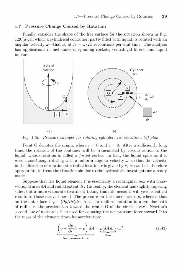
1.7—Pressure Change Caused by Rotation 39

1.7 Pressure Change Caused by Rotation

Finally, consider the shape of the free surface for the situation shown in Fig.1.20(a), in which a cylindrical container, partly filled with liquid, is rotated with anangular velocity ω—that is, at N = ω/2π revolutions per unit time. The analysishas applications in fuel tanks of spinning rockets, centrifugal filters, and liquidmirrors.

Axis ofrotation

Q

O

Pr

z

p +∂ p

∂ rdr

Cylinder wall

p

PO

ω

dr

dA

(a) (b)

ω

Fig. 1.20 Pressure changes for rotating cylinder: (a) elevation, (b) plan.

Point O denotes the origin, where r = 0 and z = 0. After a sufficiently longtime, the rotation of the container will be transmitted by viscous action to theliquid, whose rotation is called a forced vortex. In fact, the liquid spins as if itwere a solid body , rotating with a uniform angular velocity ω, so that the velocityin the direction of rotation at a radial location r is given by vθ = rω. It is thereforeappropriate to treat the situation similar to the hydrostatic investigations alreadymade.

Suppose that the liquid element P is essentially a rectangular box with cross-sectional area dA and radial extent dr. (In reality, the element has slightly taperingsides, but a more elaborate treatment taking this into account will yield identicalresults to those derived here.) The pressure on the inner face is p, whereas thaton the outer face is p + (∂p/∂r)dr. Also, for uniform rotation in a circular pathof radius r, the acceleration toward the center O of the circle is rω2. Newton’ssecond law of motion is then used for equating the net pressure force toward O tothe mass of the element times its acceleration:(

p +∂p

∂rdr − p

)dA︸ ︷︷ ︸

Net pressure force

= ρ(dAdr)︸ ︷︷ ︸Mass

rω2. (1.43)

40 Chapter 1—Introduction to Fluid Mechanics

Note that the use of a partial derivative is essential, since the pressure now variesin both the horizontal (radial) and vertical directions. Simplification yields thevariation of pressure in the radial direction:

∂p

∂r= ρrω2, (1.44)

so that pressure increases in the radially outward direction.Observe that the gauge pressure at all points on the interface is zero; in par-

ticular, pO = pQ = 0. Integrating from points O to P (at constant z):∫ pP

p=0

dp = ρω2

∫ r

0

r dr,

pP =12ρω2r2. (1.45)

However, the pressure at P can also be obtained by considering the usual hydro-static increase in traversing the path QP:

pP = ρgz. (1.46)

Elimination of the intermediate pressure pP between Eqns. (1.45) and (1.46) relatesthe elevation of the free surface to the radial location:

z =ω2r2

2g. (1.47)

Thus, the free surface is parabolic in shape; observe also that the density is not afactor, having been canceled from the equations.

There is another type of vortex—the free vortex—that is also important, incyclone dust collectors and tornadoes, for example, as discussed in Chapters 4and 7. There, the velocity in the angular direction is given by vθ = c/r, where c isa constant, so that vθ is inversely proportional to the radial position.

Example 1.8—Overflow from a Spinning Container

A cylindrical container of height H and radius a is initially half-filled with aliquid. The cylinder is then spun steadily around its vertical axis Z-Z, as shownin Fig. E1.8. At what value of the angular velocity ω will the liquid just start tospill over the top of the container? If H = 1 ft and a = 0.25 ft, how many rpm(revolutions per minute) would be needed?

1.7—Pressure Change Caused by Rotation 41

H

aaH2

H2

ω

Z Z

Z Z(a) (b)

Fig. E1.8 Geometry of a spinning container:(a) at rest, (b) on the point of overflowing.

Solution

From Eqn. (1.47), the shape of the free surface is a parabola. Therefore, theair inside the rotating cylinder forms a paraboloid of revolution, whose volume isknown from calculus to be exactly one-half of the volume of the “circumscribingcylinder,” namely, the container.8 Hence, the liquid at the center reaches thebottom of the cylinder just as the liquid at the curved wall reaches the top of thecylinder. In Eqn. (1.47), therefore, set z = H and r = a, giving the requiredangular velocity:

ω =

√2gHa2

.

For the stated values:

ω =

√2 × 32.2 × 1

0.252= 32.1

rads

, N =ω

2π=

32.1 × 602π

= 306.5 rpm.

8 Proof can be accomplished as follows. First, note for the parabolic surface in Fig. E1.8(b), r = a whenz = H, so, from Eqn. (1.47), ω2/2g = H/a2. Thus, Eqn. (1.47) can be rewritten as:

z = Hr2

a2.

The volume of the paraboloid of air within the cylinder is therefore:

V =

∫ z=H

z=0

πr2

dz =

∫ z=H

z=0

πa2z

Hdz =

1

2πa

2H,

which is exactly one-half of the volume of the cylinder, πa2H. Since the container was initially just halffilled, the liquid volume still accounts for the remaining half.

42 Chapter 1—Introduction to Fluid Mechanics

PROBLEMS FOR CHAPTER 1

1. Units conversion—E . How many cubic feet are there in an acre-foot? Howmany gallons? How many cubic meters? How many tonnes of water?

2. Units conversion—E . The viscosity μ of an oil is 10 cP and its specificgravity s is 0.8. Reexpress both of these (the latter as density ρ) in both the lbm,ft, s system and in SI units.

3. Units conversion—E . Use conversion factors to express: (a) the gravita-tional acceleration of 32.174 ft/s2 in SI units, and (b) a pressure of 14.7 lbf/in2

(one atmosphere) in both pascals and bars.

4. Meteorite density—E . The Barringer Crater in Arizona was formed 30,000years ago by a spherical meteorite of diameter 60 m and mass 106 t (tonnes),traveling at 15 km/s when it hit the ground.9 (Clearly, all figures are estimates.)What was the mean density of the meteorite? What was the predominant materialin the meteorite? Why? If one tonne of the explosive TNT is equivalent to fivebillion joules, how many tonnes of TNT would have had the same impact as themeteorite?

5. Reynolds number—E . What is the mean velocity um (ft/s) and the Reynoldsnumber Re = ρumD/μ for 35 gpm (gallons per minute) of water flowing in a 1.05-in. I.D. pipe if its density is ρ = 62.3 lbm/ft3 and its viscosity is μ = 1.2 cP? Whatare the units of the Reynolds number?

6. Pressure in bubble—E . Consider a soap-film bubble of diameter d. If theexternal air pressure is pa, and the surface tension of the soap film is σ, derive anexpression for the pressure pb inside the bubble. Hint : Note that there are twoair/liquid interfaces.

Water in

Oilout

H

(a) (b)

pw po

Pore (enlarged)Oil-bearing stratum

Impermeable rock

WaterWellWell

Oil

Fig. P1.7 Waterflooding of an oil reservoir.

9 Richard A.F. Grieve, “Impact cratering on the earth,” Scientific American, Vol. 262, No. 4, p. 68 (1990).

Problems for Chapter 1 43

7. Reservoir waterflooding—E . Fig. P1.7(a) shows how water is pumped downone well, of depth H, into an oil-bearing stratum, so that the displaced oil thenflows up through another well. Fig. P1.7(b) shows an enlargement of an idealizedpore, of diameter d, at the water/oil interface.

If the water and oil are just starting to move, what water inlet pressure pw isneeded if the oil exit pressure is to be po? Assume that the oil completely wetsthe pore (not always the case), that the water/oil interfacial tension is σ, and thatthe densities of the water and oil are ρw and ρo, respectively.10

8. Barometer reading—M . In your house (elevation 950 ft above sea level) youhave a barometer that registers inches of mercury. On an average day in January,you telephone the weather station (elevation 700 ft) and are told that the exactpressure there is 0.966 bar. What is the correct reading for your barometer, andto how many psia does this correspond? The specific gravity of mercury is 13.57.

Unknown A

Water

SG 0.9

Fig. P1.9 Cylinder immersed in water and liquid A.

9. Two-layer buoyancy—E . As shown in Fig. P1.9, a layer of an unknownliquid A (immiscible with water) floats on top of a layer of water W in a beaker.A completely submerged cylinder of specific gravity 0.9 adjusts itself so that itsaxis is vertical and two-thirds of its height projects above the A/W interface andone-third remains below. What is the specific gravity of A? Solve the problem twoways—first using Archimedes’ law, and then using a momentum or force balance.

A

B

C

1

2

hA

hB

hC

Fig. P1.10 U-tube with immiscible liquids.

10. Differential manometer—E . The U-tube shown in Fig. P1.10 has legs ofunequal internal diameters d1 and d2, which are partly filled with immiscible liquidsof densities ρ1 and ρ2, respectively, and are open to the atmosphere at the top.

10 D.L. Katz et al., Handbook of Natural Gas Engineering, McGraw-Hill, New York, 1959, p. 57, indicates awide range of wettability by water, varying greatly with the particular rock formation.

44 Chapter 1—Introduction to Fluid Mechanics

If an additional small volume v2 of the second liquid is added to the right-handleg, derive an expression—in terms of ρ1, ρ2, v2, d1, and d2—for δ, the amountby which the level at B will fall. If ρ1 is known, but ρ2 is unknown, could theapparatus be used for determining the density of the second liquid?

Hints: The lengths hA, hB, and hC have been included just to get started; theymust not appear in the final result. After adding the second liquid, consider hC tohave increased by a length Δ—a quantity that must also eventually be eliminated.

A

B

H

Fig. P1.11 Bubble rising in a closed cylinder.

11. Ascending bubble—E . As shown in Fig. P1.11, a hollow vertical cylinderwith rigid walls and of height H is closed at both ends, and is filled with anincompressible oil of density ρ. A gauge registers the pressure at the top of thecylinder. When a small bubble of volume v0 initially adheres to point A at thebottom of the cylinder, the gauge registers a pressure p0. The gas in the bubbleis ideal, and has a molecular weight of Mw. The bubble is liberated by tappingon the cylinder and rises to point B at the top. The temperature T is constantthroughout. Derive an expression in terms of any or all of the specified variablesfor the new pressure-gauge reading p1 at the top of the cylinder.

12. Ship passing through locks—M . A ship of mass M travels uphill througha series of identical rectangular locks, each of equal superficial (bird’s-eye view)area A and elevation change h. The steps involved in moving from one lock to thenext (1 to 2, for example) are shown as A–B–C in Fig. P1.12. The lock at the topof the hill is supplied by a source of water. The initial depth in lock 1 is H, andthe density of the water is ρ.

(a) Derive an expression for the increase in mass of water in lock 1 for the sequenceshown in terms of some or all of the variables M , H, h, A, ρ, and g.

(b) If, after reaching the top of the hill, the ship descends through a similar seriesof locks to its original elevation, again derive an expression for the mass ofwater gained by a lock from the lock immediately above it.

(c) Does the mass of water to be supplied depend on the mass of the ship if: (i) ittravels only uphill, (ii) it travels uphill, then downhill? Explain your answer.

Problems for Chapter 1 45

A

B

C

H

hHM

1 2 3

Fig. P1.12 Ship and locks.

13. Furnace stack—E . Air (ρa = 0.08 lbm/ft3) flows through a furnace whereit is burned with fuel to produce a hot gas (ρg = 0.05 lbm/ft3) that flows up thestack, as in Fig. P1.13. The pressures in the gas and the immediately surroundingair at the top of the stack at point A are equal.

Air Air

A

H = 100 ft

C

Gas out

Air inFurnace

ΔhWater manometer (relative positions of levels not necessarily correct)

Gas

B

Fig. P1.13 Furnace stack.

What is the difference Δh (in.) in levels of the water in the manometer con-nected between the base B of the stack and the outside air at point C? Whichside rises? Except for the pressure drop across the furnace (which you need not

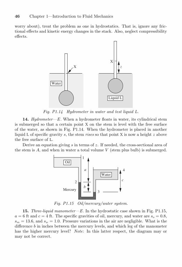
46 Chapter 1—Introduction to Fluid Mechanics

worry about), treat the problem as one in hydrostatics. That is, ignore any fric-tional effects and kinetic energy changes in the stack. Also, neglect compressibilityeffects.

zXX

Water

Liquid L

Fig. P1.14 Hydrometer in water and test liquid L.

14. Hydrometer—E . When a hydrometer floats in water, its cylindrical stemis submerged so that a certain point X on the stem is level with the free surfaceof the water, as shown in Fig. P1.14. When the hydrometer is placed in anotherliquid L of specific gravity s, the stem rises so that point X is now a height z abovethe free surface of L.

Derive an equation giving s in terms of z. If needed, the cross-sectional area ofthe stem is A, and when in water a total volume V (stem plus bulb) is submerged.

1

3

4

b

c

Mercury

a

2

Oil

Water

Fig. P1.15 Oil/mercury/water system.

15. Three-liquid manometer—E . In the hydrostatic case shown in Fig. P1.15,a = 6 ft and c = 4 ft. The specific gravities of oil, mercury, and water are so = 0.8,sm = 13.6, and sw = 1.0. Pressure variations in the air are negligible. What is thedifference b in inches between the mercury levels, and which leg of the manometerhas the higher mercury level? Note: In this latter respect, the diagram may ormay not be correct.

Problems for Chapter 1 47

16. Pressure on Mt. Erebus—M . On page 223 of the biography Shackleton (byRoland Huntford, Atheneum, New York, 1986), the Antarctic explorer’s colleague,Edward Marshall, is reported as having “ . . . fixed the altitude [of Mt. Erebus] byhypsometer. This was simply a small cylinder in which distilled water was boiledand the temperature measured. It was then the most accurate known method ofmeasuring altitude. The summit of Erebus turned out to be 13,500 feet above sealevel.”11

Assuming a uniform (mean) air temperature of −5 ◦F (the summer summittemperature is −30 ◦F), and a sea-level pressure of 13.9 psia, at what temperaturedid the water boil in the hypsometer? At temperatures T = 160, 170, 180, 190,200, and 210 ◦F, the respective vapor pressures of water are pv = 4.741, 5.992,7.510, 9.339, 11.526, and 14.123 psia.

17. Oil and gas well pressures—M . A pressure gauge at the top of an oil well18,000 ft deep registers 2,000 psig. The bottom 4,000-ft portion of the well is filledwith oil (s = 0.70). The remainder of the well is filled with natural gas (T = 60 ◦F,compressibility factor Z = 0.80, and s = 0.65, meaning that the molecular weightis 0.65 times that of air).

Calculate the pressure (psig) at (a) the oil/gas interface, and (b) the bottomof the well.

18. Thrust on a dam—E . Concerning the thrust on a rectangular dam, checkthat Eqn. (1.36) is still obtained if, instead of employing an upward coordinate z,use is made of a downward coordinate h (with h = 0 at the free surface).

19. Pressure variations in air—M . Refer to Example 1.5 concerning thepressure variations in a gas, and assume that you are dealing with air at 40 ◦F.Suppose further that you are using just the linear part of the expansion (up to theterm in z) to calculate the absolute pressure at an elevation z above ground level.How large can z be, in miles, with the knowledge that the error amounts to nomore than 1% of the exact value?

20. Grand Coulee dam—E . The Grand Coulee dam, which first operated in1941, is 550 ft high and 3,000 ft wide. What is the pressure at the base of the dam,and what is the total horizontal force F lbf exerted on it by the water upstream?

21. Force on V-shaped dam—M . A vertical dam has the shape of a V that is3 m high and 2 m wide at the top, which is just level with the surface of the waterupstream of the dam. Use two different methods to determine the total force (N)exerted by the water on the dam.

22. Rotating mercury mirror—M . Physicist Ermanno Borra, of Laval Uni-versity in Quebec, has made a 40-in. diameter telescopic mirror from a pool of

11 A more recent value is thought to be 12,450 feet.

48 Chapter 1—Introduction to Fluid Mechanics

mercury that rotates at one revolution every six seconds.12 (Air bearings elimi-nate vibration, and a thin layer of oil prevents surface ripples.)

By what value Δz would the surface at the center be depressed relative to theperimeter, and what is the focal length (m) of the mirror? The mirror cost Borra$7,500. He estimated that a similar 30-meter mirror could be built for $7.5 million.If the focal length were unchanged, what would be the new value of Δz for thelarger mirror? Hint : the equation for a parabola of focal length f is r2 = 4fz.

23. Oil and water in rotating container—E . A cylindrical container partlyfilled with immiscible layers of water and oil is placed on a rotating turntable.Develop the necessary equations and prove that the shapes of the oil/air andwater/oil interfaces are identical.

24. Energy to place satellite in orbit—M . “NASA launched a $195 millionastronomy satellite at the weekend to probe the enigmatic workings of neutronstars, black holes, and the hearts of galaxies at the edge of the universe . . . Thelong-awaited mission began at 8:48 a.m. last Saturday when the satellite’s Delta–2rocket blasted off from the Cape Canaveral Air Station.”13

This “X-ray Timing Explorer satellite” was reported as having a mass of 6,700lbm and being placed 78 minutes after lift-off into a 360-mile-high circular orbit(measured above the earth’s surface).

How much energy (J) went directly to the satellite to place it in orbit? Whatwas the corresponding average power (kW)? The force of attraction between a massm and the mass Me of the earth is GmMe/r

2, where r is the distance of the massfrom the center of the earth and G is the universal gravitational constant. Thevalue of G is not needed in order to solve the problem, as long as you rememberthat the radius of the earth is 6.37× 106 m, and that g = 9.81 m/s2 at its surface.

25. Central-heating loop—M . Fig. P1.25 shows a piping “loop” that circulateshot water through the system ABCD in order to heat two floors of a house bymeans of baseboard fins attached to the horizontal runs of pipe (BC and DA). Thehorizontal and vertical portions of the pipes have lengths L and H, respectively.

The water, which has a mean density of ρ and a volume coefficient of expansionα, circulates by the action of natural convection due to a small heater, whose inletand outlet water temperatures are T1 and T2, respectively. The pressure drop dueto friction per unit length of piping is cu2/D, where c is a known constant, u is themean water velocity, and D is the internal diameter of the pipe. You may assumethat the vertical legs AB and CD are insulated, and that equal amounts of heatare dissipated on each floor.

Derive an expression that gives the volumetric circulation rate of water, Q, interms of c, D, ρ, α, g, L, H, T1, and T2.

12 Scientific American, February 1994, pp. 76–81. There is also earlier mention of his work in Time, December15, 1986.

13 Manchester Guardian Weekly, January 7, 1996.

Problems for Chapter 1 49

A

BC

D

Heater

Fins (size exaggerated)

H

L

Flowrate, Q

Flowrate, Q

T1

T2

Fig. P1.25 Central-heating loop.

26. Pressure at the center of the earth—M . Prove that the pressure at thecenter of the earth is given by pc = 3Mgs/8πR2, in which gs is the gravitationalacceleration at the surface, M is the mass of the earth, and R is its radius. Hints:Consider a small mass m inside the earth, at a radius r from the center. The forceof attraction mgr (where gr is the local gravitational acceleration) between m andthe mass Mr enclosed within the radius r is GmMr/r

2, where G is the universalgravitational constant. Repeat for the mass at the surface, and hence show thatgr/gs = r/R. Then invoke hydrostatics.

If the radius of the earth is R = 6.37× 106 m, and its mean density is approx-imately 5,500 kg/m3, estimate pc in Pa and psi.

D

H

Wire ring

Wire ring

SoapfilmR

Fig. P1.27 Soap film on two rings.

27. Soap film on wire rings—M . As shown in Fig. P1.27, a soap film isstretched between two wire rings, each of diameter D and separated by a distanceH. Prove that the radius R of the film at its narrowest point is:

R =16

(2D +

√D2 − 3H2

).

50 Chapter 1—Introduction to Fluid Mechanics

You may assume that a section of the soap film is a circular arc, and that D ≥√3H. What might happen if D is less than

√3H?

Clearly stating your assumptions, derive an expression for the radius, in termsof D and H. Is your expression exact or approximate? Explain.

V

θ

Fig. P1.28 Person on a treadmill.

28. Treadmill stress test—M . What power P is needed to resist a force Fat a steady velocity V ? In a treadmill stress test (Fig. P1.28), you have to keepwalking to keep up with a moving belt whose velocity V and angle of inclinationθ are steadily increased. Initially, the belt is moving at 1.7 mph and has a grade(defined as tan θ) of 10%. The test is concluded after 13.3 min, at which stagethe belt is moving at 5.0 mph and has a grade of 18%. If your mass is 163 lbm:(a) how many HP are you exerting at the start of the test, (b) how many HP areyou exerting at the end of the test, and (c) how many joules have you expendedoverall?

29. Bubble rising in compressible liquid—D . A liquid of volume V and isother-mal compressibility β has its pressure increased by an amount Δp. Explain whythe corresponding increase ΔV in volume is given approximately by:

ΔV = −βV Δp.

Repeat Problem P1.11, now allowing the oil—whose density and volume areinitially ρ0 and V0—to have a finite compressibility β. Prove that the ratio of thefinal bubble volume v1 to its initial volume v0 is:

v1

v0

= 1 +ρ0gH

p0

.

If needed, assume that: (a) the bubble volume is much smaller than the oilvolume, and (b) βp0V0 � v1. If ρ0 = 800 kg/m3, β = 5.5× 10−10 m2/N, H = 1 m,p0 = 105 N/m2 (initial absolute pressure at the top of the cylinder), v0 = 10−8 m3,and V0 = 0.1 m3, evaluate v1/v0 and check that assumption (b) above is reasonable.

Problems for Chapter 1 51

A

B

H

h

C

Methane

Oil

Fig. P1.30 Well containing oil and methane.

30. Pressures in oil and gas well—M . Fig. P1.30 shows a well that is 12,000ft deep. The bottom H = 2, 000-ft portion is filled with an incompressible oil ofspecific gravity s = 0.75, above which there is an h = 10, 000-ft layer of methane(CH4; C = 12, H = 1) at 100 ◦F, which behaves as an ideal isothermal gas whosedensity is not constant. The gas and oil are static. The density of water is 62.3lbm/ft3.(a) If the pressure gauge at the top of the well registers pA = 1, 000 psig, compute

the absolute pressure pB (psia) at the oil/methane interface. Work in termsof symbols before substituting numbers.

(b) Also compute (pC − pB), the additional pressure (psi) in going from the inter-face B to the bottom of the well C.

θ

2a

W

Soapfilm

Fixedupper disk

Lower disk

2r

P (inside film)

Fig. P1.31 Soap film between two disks.

31. Soap film between disks—E (C). A circular disk of weight W and radiusa is hung from a similar disk by a soap film with surface tension σ, as shown inFig. P1.31. The gauge pressure inside the film is P .

52 Chapter 1—Introduction to Fluid Mechanics

First, derive an expression for the angle θ in terms of a, P , W , and σ. Thenobtain an equation that relates the radius of the neck r to a, P , W , and σ. Assumethat: (a) the excess pressure inside a soap film with radii of curvature r1 and r2 is2σ(1/r1 + 1/r2), and (b) the cross section of the film forms a circular arc.

32. Newspaper statements about the erg—E . In the New York Times forJanuary 18, 1994, the following statement appeared: “An erg is the metric unitscientists use to measure energy. One erg is the amount of energy it takes to movea mass of one gram one centimeter in one second.” (This statement related tothe earthquake of the previous day, measuring 6.6 on the Richter scale, in theNorthridge area of the San Fernando Valley, 20 miles north of downtown LosAngeles.)

Also in the same newspaper, there was a letter of rebuttal on January 30that stated in part: “ . . . This is not correct. The energy required to move amass through a distance does not depend on how long it takes to accomplish themovement. Thus the definition should not include a unit of time.”

A later letter from another reader, on February 10, made appropriate com-ments about the original article and the first letter. What do you think was saidin the second letter?

33. Centroid of triangle—E . A triangular plate held vertically in a liquid hasone edge (of length B) coincident with the surface of the liquid; the altitude ofthe plate is H. Derive an expression for the depth of the centroid. What is thehorizontal force exerted by the liquid, whose density is ρ, on one side of the plate?

34. Blake-Kozeny equation—E. The Blake-Kozeny equation for the pressuredrop (p1 − p2) in laminar flow of a fluid of viscosity μ through a packed bed oflength L, particle diameter Dp and void fraction ε is (Section 4.4):

p1 − p2

L= 150

(μu0

D2p

)[(1 − ε)2

ε3

].

(a) Giving your reasons, suggest appropriate units for ε.(b) If p1 − p2 = 75 lbf/in2, Dp = 0.1 in., L = 6.0 ft, μ = 0.22 P, and u0 = 0.1 ft/s,

compute the value of ε.

35. Shear stresses for air and water—E. Consider the situation in Fig. 1.8,with h = 0.1 cm and V = 1.0 cm/s. The pressure is atmospheric throughout.

(a) If the fluid is air at 20 ◦C, evaluate the shear stress τa (dynes/cm2). Does τvary across the gap? Explain.

(b) Evaluate τw if the fluid is water at 20 ◦C. What is the ratio τw/τa?(c) If the temperature is raised to 80 ◦C, does τa increase or decrease? What

about τw?

Problems for Chapter 1 53

36. True/false. Check true or false, as appropriate:14

(a) When a fluid is subjected to a steady shear stress, itwill reach a state of equilibrium in which no furthermotion occurs.

T F

(b) Pressure and shear stress are two examples of a forceper unit area.

T F

(c) In fluid mechanics, the basic conservation laws arethose of volume, energy, and momentum.

T F

(d) Absolute pressures and temperatures must be em-ployed when using the ideal gas law.

T F

(e) The density of an ideal gas depends only on its abso-lute temperature and its molecular weight.

T F

(f) Closely, the density of water is 1,000 kg/m3, and thegravitational acceleration is 9.81 m/s2.

T F

(g) To convert pressure from gauge to absolute, add ap-proximately 1.01 Pa.

T F

(h) To convert from psia to psig, add 14.7, approximately. T F

(i) The absolute atmospheric pressure in the classroomis roughly one bar.

T F

(j) If ρ is density in g/cm3 and μ is viscosity in g/cm s,then the kinematic viscosity ν = μ/ρ is in stokes.

T F

(k) For a given liquid, surface tension and surface en-ergy per unit area have identical numerical values andidentical units.

T F

(l) A force is equivalent to a rate of transfer of momen-tum.

T F

(m) Work is equivalent to a rate of dissipation of powerper unit time.

T F

(n) It is possible to have gauge pressures that are as lowas −20.0 psig.

T F

(o) The density of air in the classroom is roughly 0.08kg/m3.

T F

(p) Pressure in a static fluid varies in the vertically up-ward direction z according to dp/dz = −ρgc.

T F

14 Solutions to all the true/false assertions are given in Appendix B.

54 Chapter 1—Introduction to Fluid Mechanics

(q) At any point, the rate of change of pressure with el-evation is dp/dz = −ρg, for both incompressible andcompressible fluids.

T F

(r) A vertical pipe full of water, 34 ft high and open at thetop, will generate a pressure of about one atmosphere(gauge) at its base.

T F

(s) The horizontal force on one side of a vertical circulardisc of radius R immersed in a liquid of density ρ,with its center a distance R below the free surface, isπR3ρg.

T F

(t) For a vertical rectangle or dam of width W and depthD, with its top edge submerged in a liquid of densityρ, as in Fig. 1.15, the total horizontal thrust of theliquid can also be expressed as

∫ D

0ρghW dh, where h

is the coordinate measured downwards from the freesurface.

T F

(u) The horizontal pressure force on a rectangular damwith its top edge in the free surface is Fx. If thedam were made twice as deep, but still with the samewidth, the total force would be 2Fx.

T F

(v) A solid object completely immersed in oil will expe-rience the same upward buoyant force as when it isimmersed in water.

T F

(w) Archimedes’ law will not be true if the object im-mersed is hollow (such as an empty box with a tightlid, for example).

T F

(x) The rate of pressure change due to centrifugal actionis given by ∂p/∂r = ρr2ω, in which ω is the angularvelocity of rotation.

T F

(y) To convert radians per second into rpm, divide by120π.

T F

(z) The shape of the free surface of a liquid in a rotatingcontainer is a hyperbola.

T F

(A) The hydrostatic force exerted on one face of a squareplate of side L that is held vertically in a liquid withone edge in the free surface is F . If the plate is loweredvertically by a distance L, the force on one face willbe 3F .

T F

This page intentionally left blank

INDEX

A

Absolute pressure, 8Aggregatively fluidized beds,

560, 566fluid flow in, 569particle flow in, 468pressure distribution in,

567Analogies, between momen-

tum and heat transfer,509

Angular momentum, 81Angular velocity, 4, 39, 258,

355Annular die, flow through,

322Annular flow, 543, 552A.P.I., degrees, 11Archimedes, biographical

sketch, 36Archimedes’ law, 37Archimedes number, 200Axially symmetric irrota-

tional flow, 378

B

Balances, energy, 9, 55, 61mass, 9, 55, 57momentum, 9, 55, 78

Basis or shape function, infinite-element methods,

681Bearing, journal, 443

thrust, 443flow in, using COMSOL,

448Bernoulli, Daniel, biographi-

cal sketch, 68Bernoulli’s equation, 67, 355,

384, 533compressible flow, 161generalized, 64

Bezier curves in COMSOL,720

Bingham plastic fluids, 594,600

in pipe flow 600Blake-Kozeny equation, 207Blasius equation, 129, 428,

493, 495, 511Blasius solution for boun-

dary layer flow, 425Blow molding, 313Blunt-nosed object, flow

past, 358, 383Bob-and-cup viscometer, 627Body force, 56, 79Body-force potential, 321Boltzmann distribution, 649Boltzmann’s constant, 131Boolean operations in

COMSOL, 722Boundary, 9, 55Boundary conditions, 293Boundary layers, 414

application to turbulentjets, 513

dimensional analysis of,430

laminar, 415

simplification of equationsof motion for, 422

solution using COMSOL,435

turbulent, 428Boundary settings in COM-

SOL, 712, 724, 727Bourdon-tube pressure

gauge, 89Brinkman equation with

COMSOL, 729Brownian motion, 129Bubble caps, dynamics of, in

distillation columns, 216Bubble flow in vertical pipes,

543, 545Bubbles, in fluidized beds,

560formation at an orifice, 563rise velocity of, 562, 572

Bubbles, rise velocity of,531, 545

Bubbles, terminal velocity,532

Buckingham Pi theorem, 227Buffer region, 490Buoyancy, 36Burke-Plummer equation,

207

C

Cake, in a filter, 210Calendering, 313, 401, 450

pressure distribution in,455

743

744 Index

Capillary pressure, in porousmedium, 393

Capillary tube, for surfacetension, 19

Capillary viscometer, 623Caprock, 395Carreau model, 599, 607Cascade process in turbu-

lence, 474Centrifugal filter, 214Centrifugal pump, 164, 189Characteristic time, 596Charge number, 644“Choking” of the throat, 163Churchill, S.W., Reynolds

stress correlation, 496interpolation between two

asymptotic limits, 498Coating a moving substrate,

461Coating or spreading, 313Coaxial cylinder rheometer,

627Coefficient of contraction, 71Coefficient of discharge, 73Coefficient of thermal ex-

pansion, 12Coions, 649Colebrook and White

equation, 136, 494Commercial pipe, sizes, 138Complex piping systems, 163Composite object, COM-

SOL, 712, 723Compressibility factor, 12Compressibility, isothermal,

12Compressible flow of gases,

in a nozzle, 159in a pipeline, 156with COMSOL, 729

Compressive stress, 6Computational fluid dynam-

ics (CFD), 473, 671applications in chemical

engineering, 672COMSOL, Inc., 703, 705COMSOL Multiphysics,

examples involving,boundary-layer flow, 435

die flow, non-Newtonian,606

electroosmosis, 653, 657jet flow and mixing, 505lake flow, 373lubricated bearing, 448momentum diffusion, 307multiphysics, 653, 657orifice plate, 501parallel-plate flow, 435porous-medium flow, 705screw extruder, 318turbulent flow, 501, 505

COMSOL Multiphysics,capabilities of, 703

axes and grid settings, 710Bezier curves, 720Boolean operations, 722boundary settings,

712, 724composite object, 712, 723documentation, 705draw mode, 719draw toolbar, 711equations solvable by, 704graphical user inter-

face, 708how to run, 705interior boundariesmenus and toolbars, 709mesh, 715, 716model librarymodel navigator, 706multiphysics, 653, 657physics modes, 703plot parameters, 718postprocessing, 717problems solvable by, 725solving a problem,

717, 724subdomain settings,

714, 724surface plot, 716

Cone-and-plate viscometer,328, 626

Connate water, 392Conservation laws, 9, 55Constitutive equations,

Bingham model,594, 600

Carreau model, 599

generalized Newtonian

fluids, 598

general viscoelastic fluids,

615

Maxwell model, 615

Newtonian fluids, 296, 595

power-law model, 599

White-Metzner model, 619

Contact force, 56, 79

Continuity equation, 59, 72,

267, 268

time-averaged, 477

Control surface, 55

for momentum transfer, 81

Convection of momentum,

81

Convective derivative,

266, 619

Converging/diverging

nozzle, 159

Conversion factors, table of,

inside front cover, 25

Coriolis mass-flow meter, 95

Couette flow, 294, 312,

316, 328

in lubrication, 447

Counterions, 649

Critical pressure for com-

pressible gas flow,

158, 163

Cross product, 251

Curl of a vector, 259

expressions for, 266

Curvature, 458, 735

Curved surface, change in

pressure across, 18, 458

Cyclone separation, 219

Cylinder, flow past, compu-

ted by FlowLab,

195, 696

drag coefficient, 699

Cylindrical coordinates, 263

mass balance in, 268

momentum balances in,

322

solution of problems in,

322

Index 745

D

d’Arcy’s law, 207, 388,392, 706

Dam, force on, 32Deborah number, 596Debye-Huckel limit, 650Debye length, 650Deformation of a fluid

element, 275, 357Del (nabla) operator, in rect-

angular coordinates, 265Density, 10

◦A.P.I., 11Derivative, definition of,

27, 257Derivatives, 731Derived quantities, 225Diameter, hydraulic mean,

151Die swell, 614Dies, flow through, 313, 322

non-Newtonian, 606Differential equations,

solution of,separation of variables,

733spreadsheets, 466, 734

Differential mass balance,267

Differential momentumbalance, 271

Diffuser, in a nozzle, 159Diffusion coefficient, 15Diffusion in microchannels,

642Diffusion of momentum, 307Dilatant fluids, 593, 599, 603Dimensional analysis, 224Dimensional analysis of

boundary layer flow, 430Dimensionless groups, for

drag force, 196filtration, 224flow through packed beds,

206laminar sublayer, 230pipe flow, 132, 134pumps, 192

Dimensionless numbers,

table of, 228Dimensionless shear stress,

132, 491Dimensions, 226

mass, length, and time, 10Directional derivative, 252Discharge coefficient, 73Discretization, in numerical

methods, 674Dissipation, see frictional

dissipationDissipation, turbulent, 499

transport equation for, 500Distillation column, dynam-

ics of bubble caps, 216Dittus-Boelter equation, 511Divergence of a vector, 254

expressions for, 265Dot product, 250Double-dot product, 597Doublet, 384Drag coefficient, 196Drag coefficient on a flat

plate, 415, 419, 428,429, 432

Drag force, 194Draw mode in COMSOL,

719Draw toolbar in COMSOL,

711Drawing or spinning, 312Droplet, excess pressure

inside, 18Ducts, flow in noncircular,

150Dyadic product, 619, 740Dynamical similarity, 229

E

Eddies, 131, 474, 480formation of, 475

Eddy diffusivity, 483Eddy kinematic viscosity,

132, 482, 483, 484correlation for, 486determination of, 485in turbulent jets, 518

Eddy thermal diffusivity, 483

Eddy transport, 481Elastic modulus, 621Elastic recoil, 617Electrical double layer,

647, 648, 649Electric charge, 644

flux of, 645Electric field, 644Electric potential, 646,

649, 650Electrokinetic flow, 639, 664Electrokinetic forces, 664Electroosmosis, 647, 651

measurement of, 659Electroosmosis in a micro-

channel (COMSOL),653, 657

Electroosmotic flow around aparticle, 653

Electroosmotic mobility, 647Electrophoresis, 645, 664Electrophoretic mobility, 645Electrostatic precipitator,

202Electroviscosity, 661Energy balance, 55, 62, 598,

pipe flow, 126, 128Energy, conservation of,

9, 55English units, 22Entrance region between flat

plates, 440Eotvos number, in slug flow,

549Equations of motion, 268,

281, 294, 322, 327solutions of, 293

Equipment, visual encyclo-pedia of, 185

Equipotentials, 366in microfluidics, 656, 658

Equivalent length of fittings,154

Ergun equation, 206Euler equation, 355, 397Euler’s method, 733Eulerian viewpoint, 267Excel spreadsheets, 143, 145,

146, 150, 167, 454Extrusion of polymer, 312

746 Index

F

Falling-sphere viscometer,202

Fanning friction factor, 132,133, 135, 136, 137

Faraday’s constant, 649FEMLAB—see under its

new name, COMSOLMultiphysics

Fick’s law, 644Film flow, 456Film, in lubrication, 443Filtrate, 210Filtration, 210

centrifugal, 213plate-and-frame, 210rotary-vacuum, 212

Finite-difference methods,674

Finite-element methods, 680Finite-volume methods, 676Fittings, equivalent length,

154Five-spot pattern, 391Flooding, 555Flow energy, 62Flow, around sphere, 194

in noncircular ducts, 150in open channels, 151past a flat plate, 415, 428through a porous medium,

207through packed beds, 204

FlowLab, examplesinvolving,

flow in pipe entrance, 687flow past a cylinder, 696sudden expansion, 690two-dimensional mixing,

692FlowLab, CFD software, 682

geometry panel, 684graphical user interface,

683mesh and solve panels, 685operation toolpad buttons,

683physics, boundary

condition, and materials

panels, 684reports and postprocessing

panels, 686Flow rates, 9Flow rate, measurement of,

94by Coriolis meter, 95by orifice plate, 71by rotameter, 89

Flow regimes in two-phaseflow,

horizontal pipes, 541vertical pipes, 543

Fluent, Inc., 682Fluid, definition of, 9Fluid mechanics, laws of, 9Fluidization, 215, 559

aggregative, 560, 566particulate, 559

Fluidized bed, 559reaction in, 572

Flux, 8, 254Force, 22

as a rate of momentumtransfer, 79

on arbitrary surfaces, 33on dam, 32power for displacement of,

64units of, 21

Forced vortex, 39, 356Form drag, 194Fourier’s law, 256, 260Fox, T.R.C., xvii,

456 footnoteFree surface, 28, 33

of rotating fluid, 39Free vortex, 40, 220, 356Friction factor, 124

analogy with the Stantonnumber, 510

as a dimensionless group,132, 210

in terms of Re, 135, 491Friction-factor plot, 135Friction velocity, 489Frictional dissipation,

63, 598noncircular ducts, 151open channels, 152

packed beds, 207pipe flow, 126, 134

Froude number, in slug flow,549

Fundamental dimensions,225

G

Galerkin’s method, 681Gas constant, values of, 12Gas law, 11Gas-lift pump, 550Gas, pressure variations

in, 31Gas, underground storage

of, 395Gases, 5

flow of compressible,156, 159

viscosity of, 131Gauge pressure, 8Gate valve, 154gc, conversion factor, 22General linear viscoelastic

fluids, 615, 618Generalized Maxwell model,

618Geometrical shapes, 731Geometrical similarity, 229Globe valve, 154Gradient of a scalar, 252

expressions for, 265Graphical interface, for

COMSOL, 708

H

Hagen-Poiseuille law, 125Harrison, D., bubble forma-

tion in fluidized beds,565

Head, of fluid, 68Head/discharge curve for

centrifugal pump, 192Heat transfer, analogy with

momentum transfer,509

Index 747

Hookean solid, 616

Hoop stress in pipe wall, 139

Hydraulic mean diameter,151

Hydraulically smooth pipe,

136

Hydrostatics, 26

multiple fluids, 30

I

Impeller, of pump, 91, 190

Incipient fluidization,

215, 559

Infinite-shear viscosity, 599

Injection molding, 312

Integrals, 731

Intensity of turbulence, 477

Internal energy, 61

Invariants of the strain-rate

tensor, 597Inviscid fluid, motion of, 321Irrigation ditch, 152

Irrotational flow, 260, 356axially symmetric, 378

in cylindrical coordinates,363

in rectangular coordinates,

361

line source, 370

past a blunt-nosed object,358, 383

past a cylinder, 367

past a sphere, 386

point source, 382

stagnation flow, 369, 383

uniform flow in, 366, 380

Irrotationality condition, for

axially symmetric flow,

379

for cylindrical flow, 364

for rectangular flow, 361

Isentropic expansion, 160Isothermal compressibility,

12

Isothermal flow of gas in

pipe, 156

J

Jet mixing, COMSOLcomputation of, 505

FlowLab computation of,692

Journal bearing, 443

K

Karamanev, D.G., methodfor terminal velocities,

200Karman vortex street,

475, 697k/ε method for turbulent

flows, 499with COMSOL, 726with FlowLab, 690

Kinematic viscosity, 15, 512Kinetic energy, 61, 67

for pipe flow, 127Kinetic energy, turbulent,

499transport equation for, 500

Kolmorogov limit, 474, 476Kronecker delta, 251

L

Lagrangian viewpoint, 266Lake flow, with COMSOL,

373Lamb, Horace, feelings about

turbulence, 473Laminar flow, friction in,

frictional dissipation, 126friction factor for, 134in a pipe, 122, 123

Laminar flow, unstable,475, 700

Laminar sublayer, 155, 490dimensional analysis of,

229thickness of, 155, 493

Laminar velocity profile,124, 155

Laplace, Pierre Simon, Mar-

quis de, biographicalsketch, 362

Laplace’s equation, 262in irrotational flow, 362,

364, 379for axially symmetric flow,

379with COMSOL, 727

Laplacian operator, 262expressions for, 266

Laws of fluid mechanics, 9Leibnitz’s rule, 618 footnote,

736Leung, L.S., bubble forma-

tion in fluidized beds,565

Linear viscoelasticity, 615Line source, 370Liquids, 5Lockhart/Martinelli

correlation, 539, 552Logarithmic velocity profile,

487, 490Lorentz force, 646Loss angle, 621Loss modulus, 621Lubrication approximation,

444Lubrication flow, with COM-

SOL, 448

M

Macintosh computer forCOMSOL, 706

Magnetic settling, 662Manometer, 93Mass, 21

conservation of, 9, 55Mass balance, 55, 57

steady state, 57Mass flow rate, 9Mass velocity, 157Material types, 591MATLAB, xvi, 613, 703,

704, 706Maxwell, James Clerk, bio-

graphical sketch, 616Maxwell model, 615

748 Index

Memory function, 618Mesh refinement in

COMSOL, 715, 725Microfluidics, 639

chips for, 640Microscale fluid mechanics,

640Mist flow, 475Mixing length, correlation

for, 485determination of, 484

Mixing-length theory, 481for turbulent jets, 515

Model navigator, inCOMSOL, 706

Moment of inertia, 90Momentum, 78

angular, 90balance, 55, 78conservation of, 55, 79diffusion of, 307

Momentum balance, forbubble formation at

an orifice, 564in film flow, 405shell, 301time-averaged, 478

Momentum transfer,by convection, 9, 81by force, 79in laminar flow, 129in turbulent flow, 131

Momentum transfer, analogywith heat transfer, 509

Moody friction factor, 132

N

Natural gas, undergroundstorage of, 395

Navier, Claude-Louis-Marie-Henri, biographical

sketch, 281Navier-Stokes equations,

278, 281in microfluidics, 646with COMSOL, 725

Needle valve, 154Newton, Sir Isaac, bio-

graphical sketch, 131law of viscosity, 124, 130second law of motion,

21, 27Newtonian fluid, 4, 14, 124,

130, 275, 276, 279,591, 598

Nicklin, D.J., correlation fortwo-phase slug flow, 548

Nikuradse, pipe frictionexperiments, 136

Nonlinear simultaneousequations, 149, 166

Non-Newtonian flow in a die,with COMSOL, 606

viscosity profiles, 611Non-Newtonian flows using

COMSOL, 728Non-Newtonian fluid, 4, 592Normal stresses, 271, 276,

viscoelastic, 613Normal-stress difference, 613No-slip boundary condition,

273Nozzle, gas flow in, 159Numerical methods for

solving fluid mechanicsproblems, 673

O

Oldroyd derivative, 620One-seventh power law,

493, 495Open-channel flow, 151Order-of-magnitude

analysis,for boundary-layer flow,

423for turbulent jets, 513

Ordinary differential equa-tions, solution of, 733

Orifice, flow through,compressible, 159incompressible, 70

Orifice-plate “meter,” 71Orifice plate, COMSOL

solution, 88, 501pressure recovery, 504

Oscillatory shear, withCOMSOL, 309

Ostwald-de-Waele model,599

P

Packed beds, 204Packed-bed reactor, pressure

drop in, 208Packed column, flooding of,

556Paint films, leveling of, 463Parabolic velocity profile,

124, 155Parallel-plate rheometer, 627Particle motion in micro-

fluidic channels, 661Particles, settling of, 199,

201, 222Particulate phase (“emul-

sion”), in fluidization,560

PC for COMSOL, 706Peclet number, 643Permeability, 208, 387,

391, 396Permittivity, 646, 654Physical properties, 10Piezoelectric and piezoresis-

tive effects in pressuretransducer, 93

Piezometer, 93Piezometric tube, 69, 93Pipe fittings, pressure drop,

154Pipe flow, Bingham plastic,

604power-law fluid, 600

Pipe flow, pressure drop in,123, 133, 139

Pipe roughness, 136Pipeline, for gas, 156Pipes, flow through, 120Piping systems, 149, 163Pitot tube, 74Pitot-static tube, 74Plate-and-frame filter, 210Plot parameters in

COMSOL, 718Point source, 381Poiseuille flow, 294, 312, 316

in lubrication, 447Poisson’s equation, in

lubrication, 445

Index 749

Poisson’s equation,solution of,

by COMSOL, 373, 727by finite-element methods,

674by finite-difference

methods, 674microfluidics, 646

Polymath, 150, 164Polymer processing, 312, 450Pores, flow through, 205Porosity, 391, 396Porous medium, flow

through, 207, 566single-phase, 364, 388, 390two-phase, 390with COMSOL, 728

Potential, for porous-medium flow, 392

Potential energy, 61Potential flow, 261, 361Power,

for flowing stream, 64for force displacement, 64for pump, 64for rotating shaft, 64

Power-law fluids, 599, 600Power-law velocity profile,

495, 603Prandtl hypothesis, 486Prandtl, Ludwig, bio-

graphical sketch, 434Prandtl mixing length, 483Prandtl-Taylor analogy, 510Pressure, 6

absolute, 8gauge, 8

Pressure as a function ofheight, 26

Pressure change caused byrotation, 39

Pressure distribution, incalendering, 454

in fluidized beds, 567Pressure drop, across pipe

fittings, 154in pipe flow, 123, 133, 139

Pressure drop in two-phaseflow

horizontal pipes, 536

vertical pipes, 549, 552Pressure forces on sub-

merged objects, 36Pressure head, 68Pressure measurement, 92Pressure transducer, 93Primary recovery of oil, 390Projected area, 196Pseudoplastic fluids, 593,

599, 603Pump impeller, 91, 190Pumps, centrifugal, 164, 189

positive displacement,188, 189

Pumps in series andparallel, 193

R

Rabinowitsch equation, 624Radius of curvature, 735Rate laws, 57Rate-of-deformation tensor,

279Rate-of-strain tensor,

279, 596invariants of, 597

Reaction in fluidized bed,572

Reciprocating pumps, 188Recirculation in sudden

expansion,in jet mixing, with

FlowLab, 694using FlowLab, 691

Rectangular coordinates,249

mass balance in, 268momentum balances in,

272, 281problems in, 294

Rectangular duct, flowthrough, 150, 294

Reference quantities, 430Relaxation modulus, 618Relaxation time, 616Residual oil, 392Reynolds analogy, 509Reynolds experiment, 121

Reynolds number, 73,122, 228

for boundary-layer flow,415, 428

for drag force, 196in microfluidics, 641in pipe flow, 134, 135,

137, 149Reynolds, Osborne, bio-

graphical sketch, 121Reynolds stresses, 479

correlation for, 496Rheometers, 625Rheopectic fluids, 594Richardson-Zaki correlation,

222, 560Rod-climbing effect, 614Rotameter, 89Rotary pumps, 189Rotary-vacuum filter, 212Rotating fluid, 39Rotational flow, 356Rotational rheometers, 625Roughness, pipe, 136Rough pipe, flow in, 136, 494

S

Saturation, in porousmedium, 391

Scalars, 249Schedule number for pipe,

137Screw extruder, 313

with COMSOL, 318Secondary recovery of oil,

390Sedimentation, 222Separation of variables, 733Settling of particles, 199,

201, 222Shacham equation, for

turbulent frictionfactor, 137, 150

Shear stress, 3, 6, 14,271, 274

dimensionless groups forpipe flow, 225

distribution, 124, 300, 605

750 Index

in pipe flow, 80, 123models for, 129

Shear-thickening fluids,593, 604

Shear-thinning fluids, 593,599, 604

Shell momentum balance,301

Shock, in gas flow, 159, 163SI units, 21, 23Sign convention for stresses,

271Similar velocity profiles, 417Simple shear, 592, 597, 615Simpson’s rule, 733Simultaneous nonlinear

equations, 149, 166Slug flow in vertical pipes,

543, 547Slurry, 210Smooth pipe, flow in, 490Solenoidal flow, 256Solids, 591, 616Solution procedure, for

viscous-flow problems,293

Sound, speed of, 159, 163Source in a uniform stream,

382Specific gravity, 13Sphere, drag force on,

194, 434Sphere, flow past, 194,

386, 434Spherical coordinates, 263

mass balance in,268

momentum balances in,283

solution of problems in,327

Spherical-cap bubbles, 533Sphericity, particle, 197, 198Spinning of fibers, 325Spray drier, 201Spreadsheets, 143, 145, 146,

150, 167, 454, 734Spreadsheet solution of dif-

ferential equations, 734Spring/dashpot model, 617

Stagnation flow, 369, 383Stagnation point, 369,

383, 533Static head, 68Steady in the mean, 87, 421Steady-state energy balance,

62Steady-state mass balance,

59Steady-state problems, 57Stokes, Sir George Gabriel,

biographical sketch, 198Stokes’ law, 198Storage modulus, 621Strain rate, 592, 595, 598

for non-Newtonian flow ina die, 613

Strain-rate tensor, 279, 596Stream function, 362,

364, 378for boundary layers, 426for turbulent jets, 516, 518physical interpretation of,

364, 378Streaming potential, 659Streamlines, 57, 355, 366

in microfluidics, 656, 658Stream tube, 62Strength, of a doublet, 384

of a line source, 370of a point source, 381

Stress and strain, for visco-elastic fluid, 622

Stress, compressive, 6tensile, 5

Stress, sign convention for,271

Stress relaxation, 617Stress tensor, 274, 279, 595Strong conservation form,

673, 676Strouhal number, 699Subdomain settings in

COMSOL, 714, 724Substantial derivative, 266Sudden expansion, after

orifice plate, 86in a pipe, 88solved by FlowLab, 690

Superficial velocity, 205

Supersonic velocity, 159, 162Surface energy, 17Surface plot in COMSOL,

716Surface roughnesses, 136Surface tension, 16

in thin-film flow, 456methods for measuring, 19

Surface waves, 396Surroundings, 9, 55System, 9, 55

T

Tangential stresses, 6,272, 274

Tank draining, 70evacuation, 58filling, 76

Taylor dispersion, 642Taylor, Geoffrey Ingram,

biographical sketch, 534Taylor’s expansion, 31, 733Tensile stress, 5Tensors, 274, 279, 595, 740

“divergence” of, 741“Laplacian” of, 741

Terminal velocities ofspheres, 199

Karamanev method, 200Tertiary recovery of oil, 390Thermal diffusivity, 512Thermal expansion,

coefficient of, 12Thin films, 456Thixotropic fluids, 594Thrust bearing, 443Time-averaged continuity

equation, 477momentum balance, 478

Time-averaging, 476Torque, 91, 191

power for rotation of, 64Total head, 69Transducer, for measuring

pressure, 93Transient problems, 57Transient viscous diffusion

of momentum

Index 751

(COMSOL), 307Transition flow, 121Turbulence, 122, 124, 473

computation by the k/εmethod, 499

intensity of, 477k/ε method for, 499mixing-length theory, 481momentum transport in,

131, 480, 509orifice-plate flow, 501solved by COMSOL, 726solved by FlowLab,

690, 692velocity profiles, 155,

487, 490, 492Turbulent boundary layers,

428Turbulent core, 155, 229,

490, 492Turbulent energy, 474, 499

dissipation rate ε, 499fluctuations, 475, 476, 479

Turbulent jets, 513axisymmetric, 519plane, 514

Turbulent properties com-puted by COMSOL,

dissipation, 503, 508kinematic viscosity, 503,

507kinetic energy, 503, 508

Turbulent transport,summary of, 483

Two-phase flow in porousmedia, 390

Two-phase flow in pipes,horizontal pipes, 536vertical pipes, 543

U

Underground flow of water,364, 388

Underground storage ofnatural gas, 395

Unit vectors, 250Universal velocity profile,

488

Unstable laminar flow,475, 700

Unsteady-state problems, 57Usagi, R., interpolation

between two asymptoticlimits, 498

V

Valve, for pipeline, 154Vanes, of centrifugal pump,

190Variable-viscosity momen-

tum balance, 284Vector components, 250Vector differentiation, 251Vectors, 249

addition and subtraction,250

dyadic product, 740multiplication, 250

Velocity, 8Velocity head, 68Velocity, no-slip boundary

condition, 293Velocity of sound, 159, 162Velocity potential, 260,

361, 364, 379Velocity profiles, boundary-

layer flow, 417, 418,426, 428

calendering, 453, 463concentric cylinders, 4development in entrance

region, 440lubrication, 444parallel plates, 14pipe flow, 124, 155,

487, 490turbulent flow, 487,

490, 492turbulent jets, 517, 520viscous flow, 124, 297,

305, 316, 324, 331Vena contracta, 71Viscoelastic fluids, 613, 618

constitutive equations, 613phase relations, 622, 623

Viscometers, 625

Viscosity, 3, 13eddy kinematic, 131, 483kinematic, 15, 512of gases, 131

Viscous dissipation function,598

Viscous drag, 194Viscous-flow problems, 292Viscous modulus, 621Visual encyclopedia of

chemical engineeringequipment, 185

Void fraction, 205in two-phase flow,

536, 544, 549Volumetric flow rate, 9Volute chamber, 190Von Karman hypothesis, 487Vortex, forced, 39, 356

free, 40, 356Vortex formation during jet

mixing, 506Vortex lines, 355Vortex shedding past a

cylinder, 698Vorticity, 260, 355, 358

for non-Newtonian flowin a die, 612

source term for, 373

W

Waterflooding, 391Wave motion in deep water,

396paths followed by

particles, 399Weight, 21Weir, in distillation column,

217Weissenberg effect, 614Weissenberg, lectures of, 592Weissenberg rheo-

goniometer, 328, 626Wetted perimeter, 150Weymouth equation, 157White-Metzner model, 619Work, 56, 61

752 Index

Y

Yield stress, 594, 600

Z

Zajic, S.C., Reynolds stresscorrelation, 496

Zero-shear boundarycondition, 294

Zero-shear viscosity, 599Zeta potential, 647, 649, 651Zoom extents, 375, 501, 506