1

Fluid Mechanics3rd Year Mechanical Engineering

Prof Brian Launder

Lecture 10

The Equations of Motion for Steady Turbulent Flows

2

Objectives

• To obtain a form of the equations of motion designed for the analysis of flows that are turbulent.

• To understand the physical significance of the Reynolds stresses.

• To learn some of the important differences between laminar and turbulent flows.

• To understand why the turbulent kinetic energy has its peak close to the wall.

3

The strategy followed

• We adopt the strategy advocated by Osborne

Reynolds in which the instantaneous flow

properties are decomposed into a mean and a

turbulent part. (For the latter, Reynolds used the

term sinuous.)

• We shall mainly use tensor notation for

compactness but present the boundary layer form

in Cartesian coordinates. (Tensors hadn’t been

invented in Reynolds’ time.)

4

Preliminaries

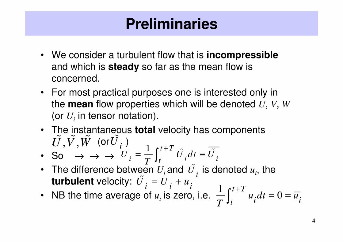
• We consider a turbulent flow that is incompressibleand which is steady so far as the mean flow is

concerned.

• For most practical purposes one is interested only in the mean flow properties which will be denoted U, V, W

(or Ui in tensor notation).

• The instantaneous total velocity has components . (or )

• So → → →

• The difference between Ui and is denoted ui, the

turbulent velocity:

• NB the time average of ui is zero, i.e.

, ,U V W% % %i

U%1 t T

i i itU U dt U

T

+= ≡∫ % %

iU%

10

t T

i itu dt u

T

+= =∫

i i iU U u= +%

5

An important point to note

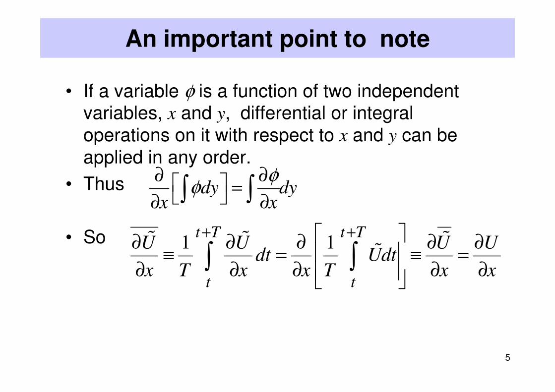
• If a variable φ is a function of two independent variables, x and y, differential or integral

operations on it with respect to x and y can be

applied in any order.

• Thus

• So

dy dyx x

φφ

∂ ∂ = ∂ ∂∫ ∫

1 1t T t T

t t

U U U Udt Udt

x T x x T x x

+ + ∂ ∂ ∂ ∂ ∂ ≡ = ≡ =

∂ ∂ ∂ ∂ ∂ ∫ ∫

% % %%

6

Averaging the equations of motion

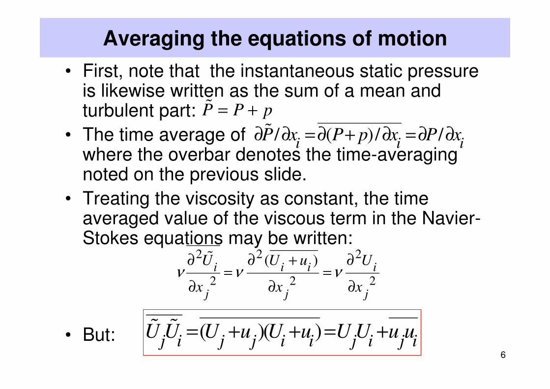
• First, note that the instantaneous static pressure is likewise written as the sum of a mean and turbulent part:

• The time average of ,

where the overbar denotes the time-averaging noted on the previous slide.

• Treating the viscosity as constant, the time averaged value of the viscous term in the Navier-Stokes equations may be written:

• But:

P P p= +%

2 2 2

2 2 2

( )i i i i

j j j

U U u U

x x xν ν ν

∂ ∂ + ∂= =

∂ ∂ ∂

%

( )( )j i j j i i j i j i

U U U u U u U U u u= + + = +% %

/ ( )/ /i i i

P x P p x P x∂ ∂ =∂ + ∂ =∂ ∂%

7

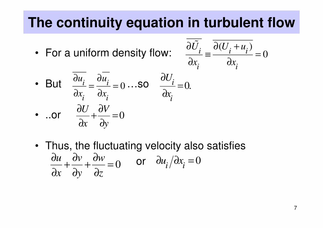
The continuity equation in turbulent flow

• For a uniform density flow:

• But …so

• ..or

• Thus, the fluctuating velocity also satisfies

or

0i i

i i

u u

x x

∂ ∂= =

∂ ∂

( )0i i i

i i

U U u

x x

∂ ∂ +≡ =

∂ ∂

%

0.i

i

U

x

∂=

∂

0U V

x y

∂ ∂+ =

∂ ∂

0u v w

x y z

∂ ∂ ∂+ + =

∂ ∂ ∂0

i iu x∂ ∂ =

8

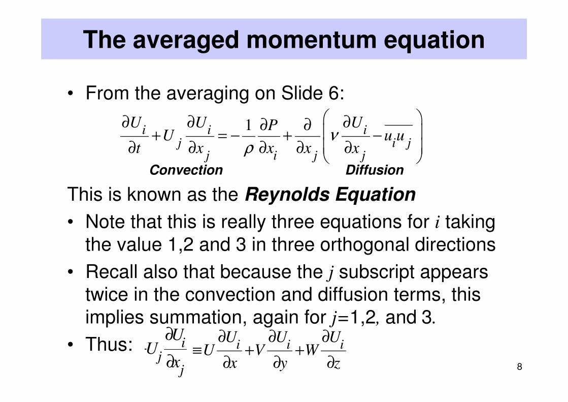
The averaged momentum equation

• From the averaging on Slide 6:

Convection Diffusion

This is known as the Reynolds Equation

• Note that this is really three equations for i taking

the value 1,2 and 3 in three orthogonal directions

• Recall also that because the j subscript appears

twice in the convection and diffusion terms, this

implies summation, again for j=1,2, and 3.

• Thus:

1i i ij i j

j i j j

U U UPU u u

t x x x xν

ρ

∂ ∂ ∂∂ ∂ + = − + − ∂ ∂ ∂ ∂ ∂

i i ij i j

j i j j

U U UU uu

t x x x x

∂ ∂ ∂+ =− + −

∂ ∂ ∂ ∂ ∂i i i

U U UU V W

x y z

∂ ∂ ∂≡ + +

∂ ∂ ∂

9

Boundary Layer form of the Reynolds Equation

• The form of the Reynolds equation appropriate to a steady 2D boundary layer is taken directly from the laminar form with

the inclusion of the same component of turbulent and viscous stress: i.e.

• The accuracy of this boundary layer model is, for some flows,

rather less than for the laminar flow case (i.e. the neglected

terms are less “negligible”).

• The form:

is a higher level of approximation (explanation given in lecture).

1 dPU U UU V uv

x y dx y yν

ρ∞ ∂ ∂ ∂ ∂

+ = − + − ∂ ∂ ∂ ∂

0U V

x y

∂ ∂+ =

∂ ∂

1 dPU U UU V uv

x y dx y yν

ρ∞ ∂ ∂ ∂ ∂

+ = − + − ∂ ∂ ∂ ∂

2 2u v

x

∂ − − ∂

10

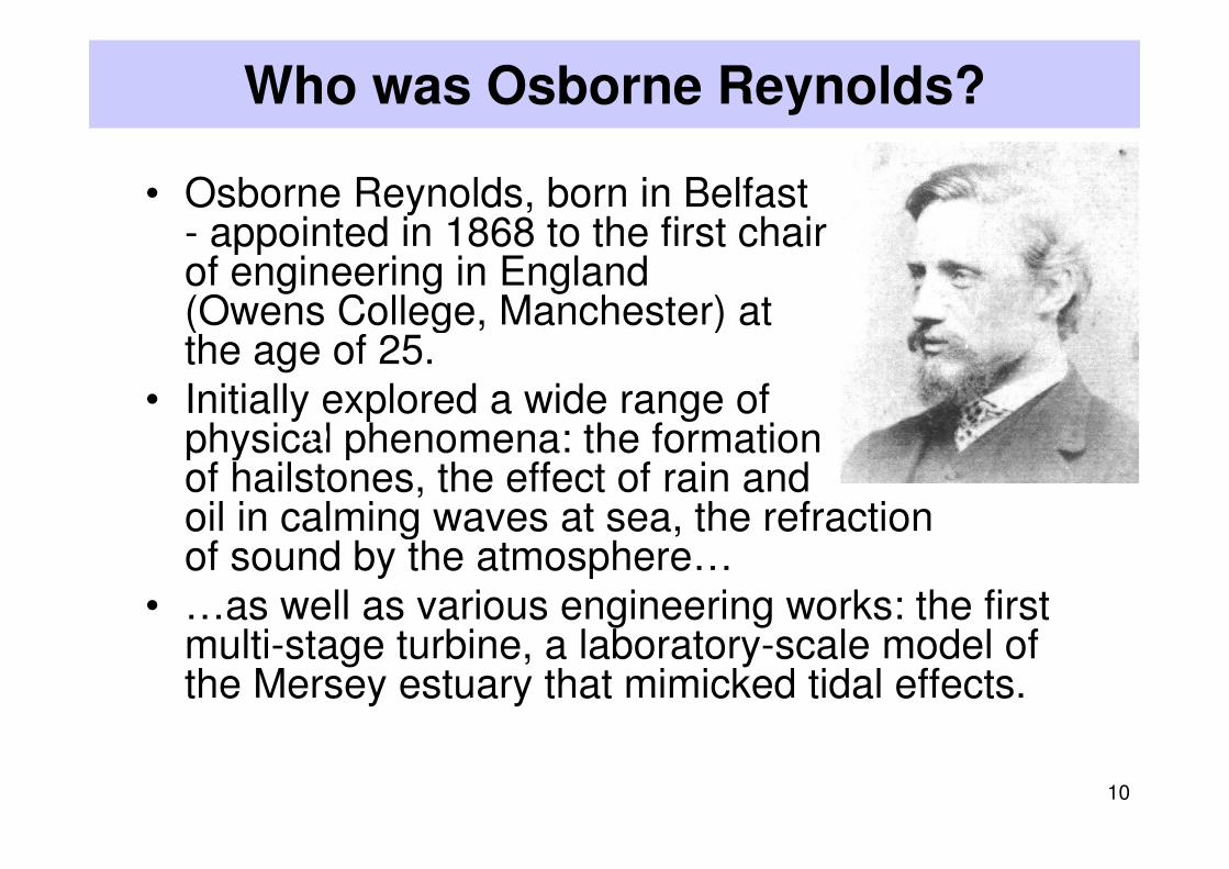
Who was Osborne Reynolds?

• Osborne Reynolds, born in Belfast - appointed in 1868 to the first chair of engineering in England (Owens College, Manchester) at the age of 25.

• Initially explored a wide range of physical phenomena: the formation of hailstones, the effect of rain and oil in calming waves at sea, the refraction of sound by the atmosphere…

• …as well as various engineering works: the first multi-stage turbine, a laboratory-scale model of the Mersey estuary that mimicked tidal effects.

O

11

Entry into the details of fluid motion

• By 1880 he had become fascinated by the detailed mechanics of fluid motion…..

• ….especially the sudden transition between direct and sinuous flow which he found occurred when: UmD/ν ≅ 2000.

• Submitted ms in early 1883 – reviewed by Lord Rayleigh and Sir George Stokes and published with acclaim. Royal Society’s Royal Medal in 1888.

12

Reynolds attempts to explain behaviour

• In 1894 Reynolds presented orally his theoretical ideas to

the Royal Society then submitted a written version.

• This paper included “Reynolds

averaging” (or, rather, mass-

weighted averaging), Reynolds

stresses and the first derivation of the turbulence energy

equation.

• But this time his ideas only

published after a long battle with the referees (George

Stokes and Horace Lamb –

Prof of Maths, U. Manchester)

13

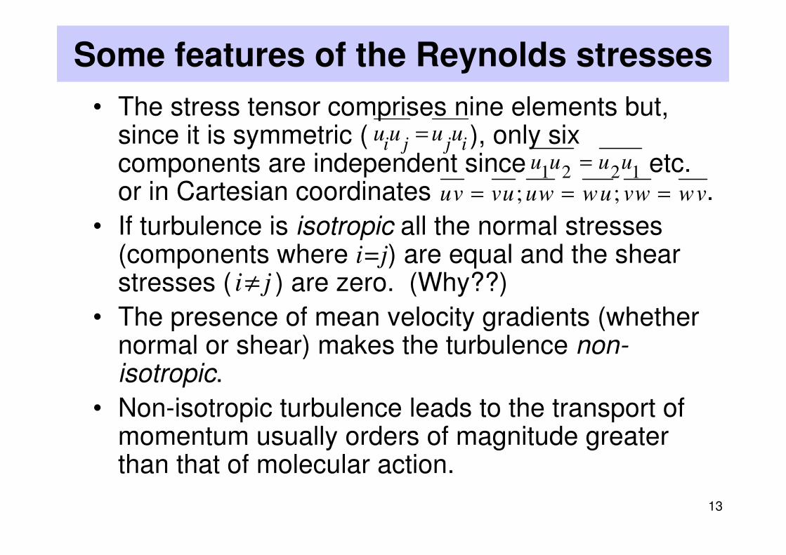
Some features of the Reynolds stresses

• The stress tensor comprises nine elements but, since it is symmetric ( ), only six components are independent since etc. or in Cartesian coordinates .

• If turbulence is isotropic all the normal stresses (components where i=j) are equal and the shear stresses ( ) are zero. (Why??)

• The presence of mean velocity gradients (whether normal or shear) makes the turbulence non-isotropic.

• Non-isotropic turbulence leads to the transport of momentum usually orders of magnitude greater than that of molecular action.

i j j iu u u u=

i j≠

1 2 2 1u u u u=

; ;uv vu uw wu vw wv= = =

14

More features of the Reynolds stresses

• Turbulent flows unaffected by walls (jets, wakes)

show little if any effect of Reynolds number on

their growth rate (i.e. they are independent of ν).

• Turbulent flows (like laminar flows) obey the no-

slip boundary condition at a rigid surface. This

means that all the velocity fluctuations have to

vanish at the wall.

• So, right next to a wall we have to have a viscous

sublayer where momentum transfer is by

molecular action alone;

• The presence of this sublayer means that growth

rates of turbulent boundary layers will depend on

Reynolds number.

0.i j

u u =

15

Comparison of laminar and turbulent boundary layers

Laminar B.L.Laminar B.L.Laminar B.L.Laminar B.L.

�Recall: The very steep near-wall velocity gradient in a turbulent b.l. reflects the damping of turbulence as the wall is approached

�But why do turbulent velocity fluctuations peak so very close to the wall?

16

The mean kinetic energy equation

• By multiplying each term in the Reynolds equation by Ui we create an equation for the mean kinetic energy:

• The left side is evidently:

or, with K≡Ui2 /2,

• Re-organize the right hand side as:

�

A B C D E

� See next slide for physical meaning of terms

i i ij i j

j i

i i

j

i

j

iU U UP

U uU U

ut x x

U

x x

Uν

ρ

∂ ∂ ∂ ∂∂ + =− + − ∂ ∂ ∂ ∂ ∂

2 22 2

i ij

j

U UU

t x

∂ ∂+ =

∂ ∂

22 2

2

2i i i i

i i j i ji j j jj

U P U U UU u u u u

x x x xxν ν

∂ ∂ ∂ ∂∂ + − − + ∂ ∂ ∂ ∂ ∂

DK

Dt=

17

The “source” terms in the mean k.e eqn

• A: Reversible working on fluid by pressure

• B: Viscous diffusion of kinetic energy

• C: Viscous dissipation of kinetic energy

• D: Reversible working on fluid by turbulent stresses

• E: Loss of mean kinetic energy by conversion to turbulence energy

18

A Query and a Fact

• Question: How do we know that term E represents a loss of mean kinetic energy to turbulence?

• Answer: Because the same term (but with an opposite sign) appears in the turbulentkinetic energy equation!

• The mean and turbulent kinetic energy equations were first derived by Osborne Reynolds.

19

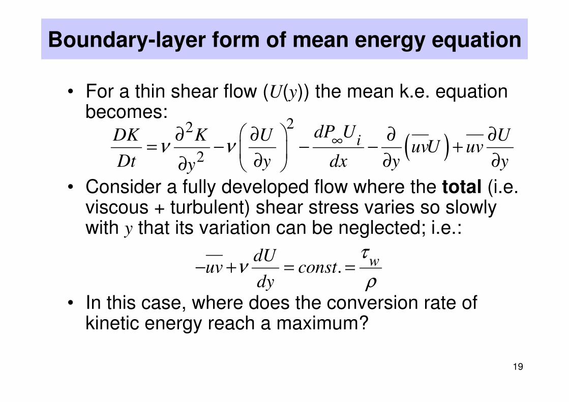
Boundary-layer form of mean energy equation

• For a thin shear flow (U(y)) the mean k.e. equation becomes:

• Consider a fully developed flow where the total (i.e. viscous + turbulent) shear stress varies so slowly with y that its variation can be neglected; i.e.:

• In this case, where does the conversion rate of kinetic energy reach a maximum?

( )22

2

idP UDK K U U

uvU uvDt y dx y yy

ν ν ∞ ∂ ∂ ∂ ∂= − − − +

∂ ∂ ∂∂

. wdUuv const

dy

τν

ρ− + = =

20

Where is the conversion rate of mean energy to turbulence energy greatest?

• This occurs where:

or where

or:

or, finally:

�Thus, the turbulence energy creation rate is a maximum where the viscous and turbulent shear stresses are equal

0d dU

uvdy dy

=

2

20

d U dU d uvuv

dy dydy+ =

2

2

( )0w

d dU dyd U dUuv

dy dydy

ν τ ρ−+ =

2

20

d U d Uu v

d yd yν

+ =

21

The near wall peak in turbulence explained

• The peak in turbulence

energy occurs very close to

the point where the transfer

rate of mean energy to

turbulence is greatest

• This occurs where viscous

and turbulent stresses are

equal – i,e. within the

viscosity affected sublayer!

• Why the turbulent velocity

fluctuations are so different

in different directions will

be examined in a later

lecture.

22

Extra slides

• The following slides provide a derivation of the

kinetic energy budget from the point of view of the

turbulence.

• They confirm the assertion made earlier that the

term represents the energy source of

turbulence.

• We do not work through the slides in the lecture (Dr

Craft will provide a derivation later) but the path

parallels that for obtaining the mean kinetic energy.

i j i ju u U x− ∂ ∂

23

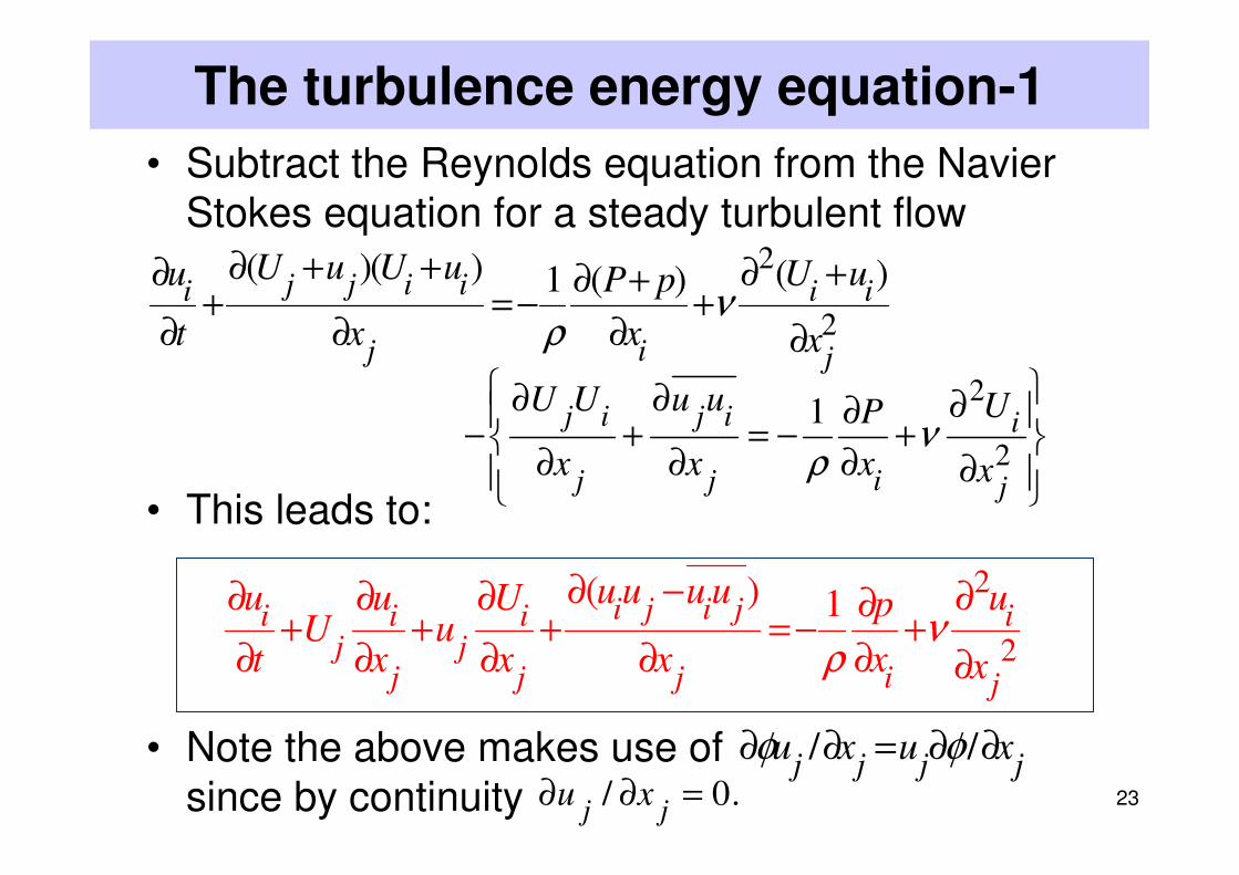
The turbulence energy equation-1

• Subtract the Reynolds equation from the Navier

Stokes equation for a steady turbulent flow

• This leads to:

• Note the above makes use of

since by continuity

2

2

1j i j i i

j j i j

U U u u UP

x x x xν

ρ

∂ ∂ ∂∂ − + = − +

∂ ∂ ∂ ∂

2

2

( )( ) ( )1 ( )j j i ii i i

j i j

U u U uu U uP p

t x x xν

ρ

∂ + +∂ ∂ +∂ ++ =− +

∂ ∂ ∂ ∂

2

2

( ) 1i j i ji i i ij j

j j j i j

u u u uu u U upU u

t x x x x xν

ρ

∂ −∂ ∂ ∂ ∂∂+ + + = − +

∂ ∂ ∂ ∂ ∂ ∂

/ /j j j j

u x u xφ φ∂ ∂ = ∂ ∂/ 0.

j ju x∂ ∂ =

24

The turbulence energy equation - 2

• Multiply the boxed equation from the previous slide by and time average.

• Note: where k is the turbulent

kinetic energy:

• The viscous term is transformed as follows:

• ε ≡ turbulence energy dissipation rate

2

2

( ) 1i i j i ji i i i i i i ij i j

j j j i j

u u u u uu u u u U u p u uU u u

t x x x x xν

ρ

∂ −∂ ∂ ∂ ∂ ∂+ + − = − +

∂ ∂ ∂ ∂ ∂ ∂

uuuuur

iu

2/ 2

i i iu u u k

t t t

∂ ∂ ∂= ≡

∂ ∂ ∂

{ }2 2 21 2 3

2k u u u≡ + +

2

2

i i i ii i

j j j j jj

u u u u ku u

x x x x x xjxν ν ν ν ε

∂ ∂ ∂ ∂ ∂ ∂ ∂ = − ≡ − ∂ ∂ ∂ ∂ ∂ ∂∂

25

The turbulence energy equation - 3

• After collecting terms and making other minor

manipulations we obtain:

viscous turbulent diffusion generation dissipation

• Note this is a scalar equation and each term has to

have two tensor subscripts for each letter.

• Repeat Q & A: How do we know that

represents the generation rate of turbulence? Ans:

The same term but with opposite sign appears in

the mean kinetic energy equation.

2[ / 2 ]i i

i j ij i jj j j

pu UDk ku u u u

Dt x x xν δ ε

ρ

∂∂ ∂ = − + − −

∂ ∂ ∂

[ / 2 ]i ii j ij i j

j j j

pu Uu u u u

Dt x x xν δ ε = − + − −

∂ ∂ ∂

/i j

U x∂ ∂

26

A question for you

• Compile a sketch of the mean kinetic energy budget for fully developed laminarflow between parallel planes.