fluid-rock characterization for nmr well logging …gjh/consortium/resources/doe-nmr...fluid-rock...
TRANSCRIPT

Fluid-Rock Characterization for NMR Well Logging andSpecial Core Analysis
2nd Annual Report
October 1, 2005 – September 30, 2006
George J. Hirasaki ([email protected])
and
Kishore K. Mohanty ([email protected])
Issued: February 2007
DE-FC26-04NT15515
Project Officer:Chandra Nautiyal, Tulsa
Contract Officer:Thomas J. Gruber, Pittsburg
Rice University6100 Main Street
Houston, TX 77005
University of Houston4800 Calhoun Road
Houston, TX 77204-4004

2
DISCLAIMER* — The Disclaimer must follow the title page, and must contain thefollowing paragraph:
"This report was prepared as an account of work sponsored by an agencyof the United States Government. Neither the United States Government nor anyagency thereof, nor any of their employees, makes any warranty, express orimplied, or assumes any legal liability or responsibility for the accuracy,completeness, or usefulness of any information, apparatus, product, or processdisclosed, or represents that its use would not infringe privately owned rights.Reference herein to any specific commercial product, process, or service by tradename, trademark, manufacturer, or otherwise does not necessarily constitute orimply its endorsement, recommendation, or favoring by the United StatesGovernment or any agency thereof. The views and opinions of authorsexpressed herein do not necessarily state or reflect those of the United StatesGovernment or any agency thereof."

3
ABSTRACT
Abstract for Project
NMR well logging provides a record of formation porosity, permeability,irreducible water saturation, oil saturation and viscosity. In the absence offormation material, the NMR logs are interpreted using default assumptions.Special core analysis on core samples of formation material provides acalibration between the log response and the desired rock and/or fluid property.The project proposes to develop interpretations for reservoirs that do not satisfythe usual assumptions inherent in the interpretation. Also, NMR will be used inspecial core analysis to investigate the mechanism of oil recovery by wettabilityalteration and the relative permeability of non-water-wet systems.
Some common assumptions and the reality of exceptional reservoirs arelisted in the following and will be addressed in this project.
(1) Assumption: in situ live crude oil and OBM have a relaxation timeproportional to temperature/viscosity as correlated from stock tank oils.Reality: methane and ethane relax by a different mechanism than for deadoil and GOR is a parameter; carbon dioxide does not respond to protonNMR but influences oil and gas viscosity and relaxation rates.
(2) Assumption: the in situ hydrocarbons have a relaxation time equal to thatof the bulk fluid, i.e. there is no surface relaxation as if the formation iswater-wet. Reality: Most oil reservoirs are naturally mixed-wet and drillingwith oil-based mud (OBM) sometimes alters wettability. If the formation isnot water-wet, surface relaxation of the hydrocarbon will result.
(3) Assumption: OBM filtrate has the properties of the base oil. Reality: OBMfiltrate often has some level of the oil-wetting additives and in some caseshas paramagnetic particles. It may also have dissolved gas.
(4) Assumption: the magnetic field gradient is equal to that of the logging tool.Reality: paramagnetic minerals may result in internal magnetic fieldgradient much greater than that of the logging tool.
(5) Assumption: pores of different size relax independently. Reality: claylined pores can have significant diffusional coupling betweenmicroporosity and macroporosity.
Abstract for 2nd-Annual ReportProgress is reported on Tasks: (1.1) Properties of live reservoir fluids,
(2.1) Extend the diffusion editing technique and interpretation, (2.4) Interpretationof systems with diffusional coupling between pores, (2.5) Quantify themechanisms responsible for the deviation of surface relaxivity from the meanvalue for sandstones and carbonates. and (3) Characterization of pore structureand wettability.
4
TABLE OF CONTENTS
DISCLAIMER..........................................................................................................2
ABSTRACT.............................................................................................................3
EXECUTIVE SUMMARY ........................................................................................5
Subtask 1.1 Properties of live reservoir fluids ......................................................... 9
Subtask 2.1 Extend the diffusion editing technique and interpretation.................... 23
Subtask 2.4 Interpretation of systems with diffusional coupling between pores......45
Subtask 2.5 Quantify the mechanisms responsible for the deviation of surfacerelaxivity from the mean value for sandstones and carbonates. ...........................59
Task 3: Characterization of pore structure and wettability. .....................................111
NMR 1-D Profiling ................................................................................................... 193

5
EXECUTIVE SUMMARY
NMR High Pressure Measurements for Natural Gas Mixtures
The work presented below shows the status of NMR high pressuremeasurements. So far, a manifold has been built for making NMRmeasurements at high pressures up to 5000 psi. Furthermore, a diffusion-editingpulse sequence has been tested at ambient pressure for appropriate criteria inchoosing parameters for the NMR measurement. The tests were done with acrude oil and suggest that a parameter selection technique developed by Flaum(2006) is appropriate, with the parameters chosen such that they apply to themode relaxation time and diffusivity (as opposed to the log-mean). This is likelyapplicable to high pressure NMR measurements of gas mixtures planned in thefuture. Finally, separate relaxation time and diffusivity measurements are shownfor methane gas at elevated pressure for comparison with values from otherinvestigators. Methane relaxation times that correspond to the expected trendfrom the literature have been obtained, but the reproducibility is suspect and isyet to be established. The diffusivity shows consistency; however the value is20% less than the correlated value from Prammer, et al.(1995). Data is notavailable at 30 ºC, the temperature in the present measurements, but a 20%deviation is within the bounds of the fit of the correlation to experimental data.
A Pulsed Field Gradient with Diffusion Editing (PFG-DE) NMR Technique forEmulsion Droplet Size Characterization
This paper describes a nuclear magnetic resonance (NMR) technique,pulsed field gradient with diffusion editing (PFG-DE), to quantify drop sizedistributions of brine/crude oil emulsions. The drop size distributions obtainedfrom this technique were compared to results from the traditional pulsed fieldgradient (PFG) technique. The PFG-DE technique provides both transverserelaxation (T2) and drop size distributions simultaneously. In addition, the PFG-DE technique does not assume a form of the drop size distribution. An algorithmfor the selection of the optimal parameters to use in a PFG-DE measurement isdescribed in this paper. The PFG-DE technique is shown to have the ability toresolve drop size distributions when the T2 distribution of the emulsified brineoverlaps either the crude oil or the bulk brine T2 distribution. Finally, the PFG-DEtechnique is shown to have the ability to resolve a bimodal drop size distribution.
NMR Diffusional Coupling: Effects of Temperature and Clay Distribution
The interpretation of Nuclear Magnetic Resonance (NMR) measurementson fluid- saturated formations assumes that pores of each size relaxindependently of other pores. However, diffusional coupling between pores ofdifferent sizes may lead to false interpretation of measurements and thereby, awrong estimation of formation properties. The objective of this study is to provide
6
a quantitative framework for the interpretation of the effects of temperature andclay distribution on NMR experiments. In a previous work, we established thatthe extent of coupling between a micropore and macropore can be quantifiedwith the help of a coupling parameter () which is defined as the ratio ofcharacteristic relaxation rate to the rate of diffusive mixing of magnetizationbetween micro and macropore. The effect of temperature on pore coupling isevaluated by proposing a temperature dependent functional relationship of .This relationship takes into account the temperature dependence of surfacerelaxivity and fluid diffusivity. The solution of inverse problem of determining and microporosity fraction for systems with unknown properties is obtainablefrom experimentally measurable quantities.
Experimental NMR measurements on reservoir carbonate rocks andmodel grainstone systems consisting of microporous silica gels of various grainsizes are performed at different temperatures. As temperature is increased, theT2 spectrum for water-saturated systems progressively changes from bimodal tounimodal distribution. This enhanced pore coupling is caused by a combinedeffect of increase in water diffusivity and decrease in surface-relaxivity withtemperature. Extent of coupling at each temperature can be quantified by thevalues of . The technique can prove useful in interpreting log data for hightemperature reservoirs.
Effect of clay distribution on pore coupling is studied for model shalysands made with fine silica sand and bentonite or kaolinite clays. The NMRresponse is measured for two cases in which clay is either present as a separate,discrete layer or homogeneously distributed with the sand. For layered systems,T2 spectrum shows separate peaks for clay and sand at 100% water saturationand a sharp T2,cutoff could be effectively applied for estimation of irreduciblesaturation. However, for dispersed systems a unimodal T2 spectrum is observedand application of 33ms T2,cutoff would underestimate the irreducible saturation inthe case of kaolinite and overestimate in the case of bentonite. The inversiontechnique can still be applied to accurately estimate the irreducible saturation.
Paramagnetic Relaxation in Sandstones: Distinguishing T1 and T2Dependence on Surface Relaxation, Internal Gradients and Dependence onEcho Spacing
Sandstones have T1/T2 ratio of 1.6, on the average. Clean silica has aT1/T2 ratio of about 1.3. If T2 changes with echo spacing in a homogeneousapplied magnetic field, the change is interpreted to be due to diffusion in internalgradients. We demonstrate that when the paramagnetic material is iron, theincrease in the T1/T2 ratio above that of clean silica is due to diffusion in internalgradient. Furthermore, when the paramagnetic sites are small enough, nodependence on echo spacing is observed with conventional low-field NMRspectrometers. Echo spacing dependence is observed when the paramagnetic

7
materials become large enough or form a ‘shell’ around each silica grain suchthat the length scale of the region of induced magnetic gradients is largecompared to the diffusion length during the time of the echo spacing.
The basis for these assertions is a series of experiments and calculationsdescribed below. A solution of hydrated Fe3+ ion has a T1/T2 ratio of unity.Aqueous dispersions of paramagnetic magnetite particles ranging from 4 nm to110 nm have T1/T2 increasing with particle size. No echo spacing dependence isobserved. Larger (25nm and 110 nm) magnetite particles coated on 50 µm silicagrains have no echo spacing dependence for lower concentration of particles butshow echo spacing dependence for larger concentrations. Largest (2,600 nm)magnetite particles mixed with fine sand have echo spacing dependence andT1/T2 greater than 2.
These experimental observations are being interpreted by theoreticalcalculations. The magnetite particles are modeled as paramagnetic spheres.Paramagnetic particles on the surface of silica grains are modeled as individualparticles at low concentrations. At high surface concentrations, they are modeledas a thin, spherical shell of paramagnetic material. Calculations show that thesystem transitions from motionally averaging (no dependence on echo spacing)to localization regime (dependent on echo spacing) at high surface concentrationof paramagnetic particles.
NMR Well Logging and Special Core Analysis for Fluid-RockCharacterization
Characterization of pore structure and wettability has been completed onsix carbonate samples. The vug size, distribution and interconnection varysignificantly in these six samples. The thin sections have been characterizedthrough their pore size distribution, two-point correlation function, chord numberdistribution, lineal path function and fractal dimension. The power spectrum fromFourier transform has been computed. The three-dimensional pore structureshave been reconstructed for two carbonates and one sandstone sample. Singlephase permeability and NMR response has been measured for all the samples.The relative permeability, NMR response and electrical conductivity have beenmeasured for three samples.
NMR 1-D Profiling
T2 profiles can be generated by implementing the rapid acquisition withrelaxation enhancement (RARE) pulse sequence. The RARE sequence is amulti-echo imaging sequence used to construct a one-dimensional profile of T2relaxation times. Experimental parameters, such as sample size, gradientstrength and duration, and the number and spacing of the acquired data points,must be selected to ensure that useful information can be extracted from theprofiles. The sample must be centered within the Maran’s sweet spot. Thegradient strength relates the precession frequency to sample position.Attenuation due to diffusion is dependent on the product of gradient strength (g)
8
and duration (d). Therefore, g and d should be selected in order to reduce theamount of the relaxation due to diffusion. The dwell time (DW), or spacingbetween acquired data points, needs to be selected so that the sample plus asmall region above and below is resolved by the experiment. The number ofdata points collected per echo will influence the image resolution; as more pointsare collected per echo, the resolution will increase. Experiments were performedon both a water sample and a layered water-squalane (C-30 oil, m = 22 cP)system using the RARE sequence. T2 was calculated by fitting the decayingprofiles to a single exponential model. The difference between the T2 profilesacquired via RARE and the T2 of the bulk samples found using CPMG is due todiffusion and thus needs to be minimized.

9
Task 1. Properties of reservoir fluidsSubtask 1.1 Properties of live reservoir fluids
NMR High Pressure Measurements for Natural Gas MixturesArjun Kurup and George Hirasaki
Abstract
The work presented below shows the status of NMR high pressuremeasurements. So far, a manifold has been built for making NMRmeasurements at high pressures up to 5000 psi. Separate relaxation time anddiffusivity measurements are shown for methane gas at elevated pressure forcomparison with values from other investigators. Methane relaxation timesapproaching the expected trend from the literature have been obtained.However the relaxation times obtained are consistently smaller than reportedvalues. The measured diffusivity is consistent within the measurements in thiswork; however the value is 20% less than the correlated value from Prammer, etal. (1995). The diffusivity data do not appear to match the correlation within thescatter of the data. The reason for this is unknown.
Introduction
This report discusses steps in preparation for making NMR measurementsof high pressure gas mixtures. The anticipated samples are mixtures ofmethane, ethane, propane, nitrogen, and carbon dioxide, components that areoften present in significant quantities in natural gas reservoirs (McCain 1990).The present document recounts measurements of relaxation times (T1 and T2)and diffusivity of methane gas, to validate the high pressure apparatus byconfirmation with values available in the literature.
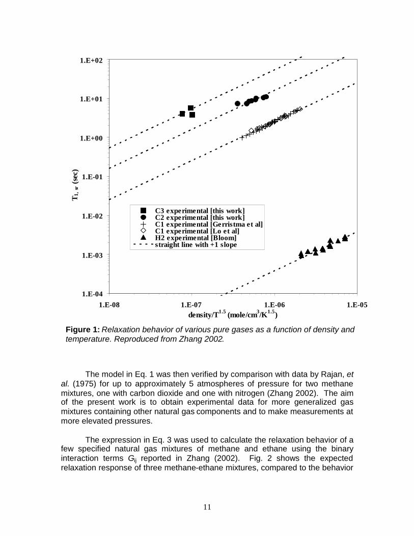
The measurements mentioned here are motivated by downhole NMRlogging measurements. NMR well-logging of gas reservoirs provides NMRresponse (some combination of relaxation times, T1 and T2, and diffusivity) as afunction of depth in the reservoir. The NMR response must then be correlated tostate properties like density and temperature. NMR properties of methane havebeen studied, both in the laboratory setting (Gerritsma et al. 1971, Lo 1999,Dawson 1966, Oosting and Trappeniers 1971, Harris 1978), and in natural gasreservoirs (Prammer et al. 1995, Akkurt et al. 1996). For the purposes ofreservoir evaluation, it has been previously assumed that the presence of non-methane components can be accounted for simply by the gas density (Akkurt etal. 1996). However as Fig. 1 shows, different gases show different NMRbehavior (T1 relaxation time in Fig. 1) for the same normalized density (Zhang2002). Thus, non-methane components of natural gas require distinct treatment.

10
Based on theory that postulates NMR relaxation results from binarycollisions between molecules (Bloom et al., 1967; Gordon, 1966), Zhang (2002)presented a model for relaxation of gas mixtures based on the relaxationbehavior of each gas in the mixture. The resulting expression is
ji
ji
ii
An
jji TkCI
NT
24 2
eff,2
2
1,1
. (1)
In this equation, T1,i is the T1 relaxation time of the ith component in the mixture, j
is the partial molar density of the j-th component of the mixture, ħis Planck’sconstant divided by 2, is Avogadro’s number, k is Boltzmann’s constant, T isthe temperature, I is the moment of inertia in the direction perpendicular to theaxis of the molecule, and Ceff is a quantity describing coupling between nuclearand molecular angular momentum. The other quantities in Eq. 1 are defined byone of the following equations (Zhang 2002),
jiji mm
11 (2.a)
and
)300()300(300 KKT iijjji . (2.b)
In Eq. 2.a, mi and mj are the atomic masses of the two colliding molecules. InEq. 2.b, refers to the collision cross-section for angular momentum transfer.
In practice, Eq. 1 can be simplified to (Zhang 2002)
n
j
ijji T
GT
15.11, (3)
where G ij is a binary interaction term that collects the constants in Eq. 1. Eq. 3does, however keep the temperature dependence explicit, incorporating thetemperature dependence of , the binary collision parameter, from Eq. 2.b.
11
The model in Eq. 1 was then verified by comparison with data by Rajan, etal. (1975) for up to approximately 5 atmospheres of pressure for two methanemixtures, one with carbon dioxide and one with nitrogen (Zhang 2002). The aimof the present work is to obtain experimental data for more generalized gasmixtures containing other natural gas components and to make measurements atmore elevated pressures.
The expression in Eq. 3 was used to calculate the relaxation behavior of afew specified natural gas mixtures of methane and ethane using the binaryinteraction terms Gij reported in Zhang (2002). Fig. 2 shows the expectedrelaxation response of three methane-ethane mixtures, compared to the behavior
1.E-04
1.E-03
1.E-02
1.E-01
1.E+00
1.E+01
1.E+02
1.E-08 1.E-07 1.E-06 1.E-05density/T1.5 (mole/cm3/K1.5)
T1,
sr(s
ec)
C3 experimental [this work]C2 experimental [this work]C1 experimental [Gerristma et al]C1 experimental [Lo et al]H2 experimental [Bloom]straight line with +1 slope
Figure 1: Relaxation behavior of various pure gases as a function of density andtemperature. Reproduced from Zhang 2002.

correlated for the individual gases. Fig. 3 shows the calculated response for amethane-ethane-propane mixture.
0.01
0.1
1
10
1.E-08 1.E-07 1.E-06Density/Temperature 1.5 (mol/cm3/K1.5)
T 1(s
)
C1-C2 Mixture 1 (20% C1) C1-C2 Mixture 2 (50% C1)
C1-C2 Mixture 3 (80% C1) C1 Correlation
C2 Correlation
Figure 2: Calculated relaxation behavior of methane(C1)-ethane(C2)
mixtures with relation to correlations for methane and ethane0.1
1
10
100
1.E-08 1.E-07 1.E-06 1.E-05Density/Temperature1.5 (mol/cm3/K1.5)
T1/
Den
sity
(s*c
m3 /m
ol)
Methane-Ethane-Propane Mixture Calc.Methane CorrelationEthane CorrelationPropane Correlation
Figure 3: Calculated relaxation behavior of methane-ethane-propane mixture(80% methane, 13.5% ethane, 6.5% propane) in possession with relation to
12
correlations for methane, ethane, and propane

13
Equipment and Capabilities
The NMR spectrometer used for the work mentioned here is a 2 MHzbench-top MARAN apparatus. It is equipped with one-dimensional gradient coils,which provides a linear spatial magnetic field gradient for use in diffusionevaluations. The pulse sequences used are standard sequences: inversionrecovery for measuring T1, CPMG for measuring T2, and a pulsed-field gradient(PFG) stimulated-echo sequence for measuring diffusivity.
For high pressure measurements with gases, a manifold was built fromstainless steel fittings, manufactured by Swagelok. A schematic of the manifoldand its ports, which form the NMR high pressure system, is shown in Fig. 4. Afew statements regarding the features of the NMR high pressure system follow.First, gas cylinders with appropriate gas or gas mixture are connected to the inletside of the apparatus. The inlet line is equipped with an oxygen scavenger(Matheson model 6411) to remove traces of oxygen from the contents of the gascylinder. Oxygen is a paramagnetic contaminant and could detrimentally affectmeasured NMR relaxation times if not removed. The oxygen scavenger is ratedfor a maximum pressure differential of 90 psi between inlet ad outlet. Second,the manifold is equipped with a vacuum line. This is used to evacuate thesystem prior to injection of gases at elevated pressure. The line is connected toa mechanical vacuum pump, with a trap, cooled by dry ice (freezing point of-78.5 ºC) in isopropanol. Furthermore, to prevent accidental exposure of thevacuum line to high pressure, the vacuum line is double-valved. The thirdfeature is the two lines to two hand pressure generation pumps (hand pumps),models 87-6-5 and 62-6-10 manufactured by High Pressure EquipmentCompany. These hand pumps can be used to increase the system pressurebeyond tank pressure by compressing the system volume. The fourth feature ofthe high pressure NMR system is the pressure gauges that allow monitoring ofpressure during NMR measurements. One gauge is a pressure transducermanufactured by Sensometrics, Inc. coupled to the manifold using an adapterand connected to a digital readout meter. Both the adapter and meter (modelDP41-S) are made by Omega. The entire system also outlets to a vent to safelyremove gases after measurements are complete. Another safety feature is therelief lines in the system. A check valve in the relief line for the vacuum portionprotects the vacuum side from overpressurization; the check valve opens to thevent line should any positive pressure occur in the vacuum line. The relief line ofthe high-pressure portion of the manifold also discharges into the vent. Howeverin this case, relief is provided by a diaphragm-type blowout valve manufacturedby Autoclave Engineers, where the diaphragm is designed to yield at pressuresgreater than 5000 psi. The final component of the system is the NMR pressurevessel, manufactured by Temco, Inc. It will be described in the followingparagraph. A photograph of the NMR high pressure system is shown in Fig. 5.The system is rated to 5000 psi pressure, except the vacuum line (designed forrunning at subatmospheric pressure) and the inlet line, where the gas cylinder is
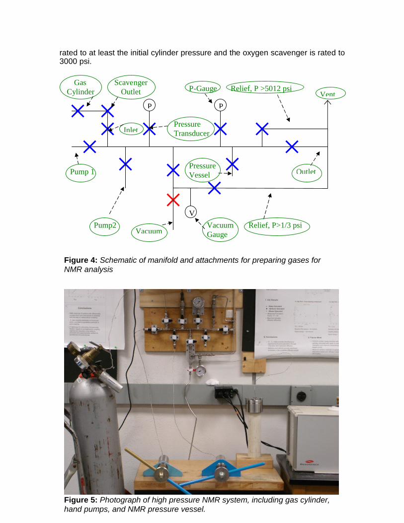
14
rated to at least the initial cylinder pressure and the oxygen scavenger is rated to3000 psi.
P
V
InletPressureTransducer
P-Gauge Relief, P >5012 psi
Pump 1
Pump2Vacuum
PressureVessel
Relief, P>1/3 psi
Outlet
Vent
VacuumGauge
GasCylinder
P
ScavengerOutlet
Figure 5: Photograph of high pressure NMR system, including gas cylinder,hand pumps, and NMR pressure vessel.
Figure 4: Schematic of manifold and attachments for preparing gases forNMR analysis

15
The NMR pressure vessel is the component of the high pressure NMRsystem that is placed in the MARAN 2 MHz instrument to make NMRmeasurements. A diagram of the design of the NMR pressure vessel is shown inFig. 6. As shown, the pressure vessel has three layers. The outermost layer isthe pressure-bearing surface, made of fiberglass in an epoxy matrix. The middlelayer seals the system and connects it to the manifold. The top of this portion ofthe NMR pressure vessel is a stainless steel flange. The flange has ports at thetop which connect to a line from the manifold and o-rings that contact the insideof the PEEK liner. The PEEK liner is the body of the NMR pressure vessel, asthe inner layer is contained inside it. The middle layer is sealed at the bottomwith a stainless steel end piece capped with an o-ring. The inner layer consistsof two PEEK cylinders, one that allows gas to pass along a small orifice along itsaxis and the other serving as a sample chamber (which is aligned in themagnetic field of the MARAN 2 MHz instrument) with a hollow region ofapproximately 12.9 ml where the measured gas resides. The NMR pressurevessel, like the manifold is rated to 5000 psi.
Prior to use, the manifold and pressure vessel were tested under pressure. First,the NMR high pressure system was tested with water in the system. Pressuresup to 5000 psig were achieved. The high-pressure relief line was found to
Figure 6: Drawing of Temco ® NMR pressure vessel

16
operate correctly during this test because the diaphragm failed (as designed) atslightly beyond 5000 psig. The manifold, without the NMR pressure vessel, wasfound to maintain pressure when tested under pressure at 4500 psig. However,when the NMR pressure vessel is incorporated, a leak of approximately 10 psi/hris presently being observed at pressures near 2000 psia. Several attempts tostop the leak have proven unsuccessful. Nonetheless, the magnitude of the leakwas deemed to be acceptable for measurements to proceed. This assessmentcan be made by calculating the effect of variations in pressure (due to the leak)on NMR measurements. When this calculation was made, the difference in NMRmeasurements (of relaxation times or diffusivity) was found to be 2% or less forthe majority of the pressure variations observed so far. (This determination wasmade using Eqs. 4 and 5, shown in the following section.) Thus, the effect of theleak is deemed to be acceptable for NMR measurements.
Elevated Pressure NMR Measurements with Methane
Using the high pressure NMR apparatus shown in Figs. 4-6, NMRmeasurements are currently in progress with methane gas. NMR T1, T2, anddiffusion measurements have been performed. Data for methane are available inthe literature, and the purpose of the present methane measurements isvalidation of the apparatus described in the previous section. Relaxation timemeasurements thus far have fallen within approximately 10% of the expectedvalue, but show a bias toward short relaxation times. It appears that oxygen(paramagnetic contaminant) is still present in the methane sample for the casesconsidered. Diffusion measurements provide a methane diffusivity that isapproximately 20% below the expected correlation, the reason for which is yet tobe determined.
Before taking the data obtained into consideration, the default proceduresused to prepare the high pressure NMR apparatus for making a gasmeasurements follow:
1. Evacuation of system to remove air, especially to reduce oxygen content.(This step is disregarded in cases where an experiment begins at anelevated pressure obtained in a previous measurement.)
2. Pressurization to small elevated pressure (typically approximately 500 psi)and purging this pressure to slightly above atmospheric pressure (typicallyapproximately 20-50 psig). This step is repeated for a desired number ofrounds (typically 3-5 rounds)
3. Pressurization of system to up to gas cylinder pressure, controlling the gascylinder regulator pressure.
4. Final pressurization using the hand pressure generation pumpsNote that steps 2 and 3 must be performed carefully to allow any oxygen in themethane sample enough time to contact the oxygen scavenger. Once the stepsabove are taken, the sample is ready for NMR measurements.

17
In relaxation time (T1 and T2) measurements, the response of NMR signalamplitude is measured as a function of time. The resultant data is said to be inthe time domain. The acquired data is then inverted, converting the time-domaindata to the relaxation time (T1 or T2) domain. For T2, the large number of time-domain data points is parsed before the conversion to the T2-domain isperformed. The parsing process, called “sampling and averaging”, reduces thecomputational load in the conversion with minimal sacrifice to data quality(Chuah 1996). Due to fewer data points in T1 measurements, no parsingprocess is necessary.
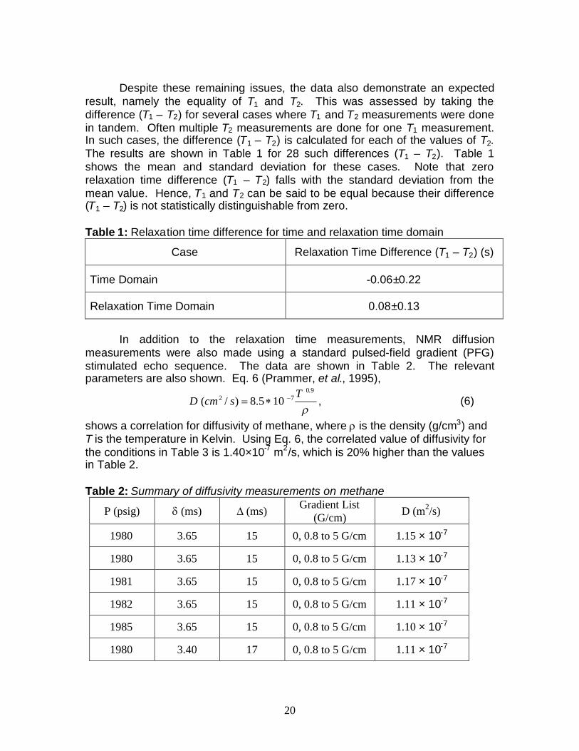
The time domain data obtained thus far show an anomaly illustrated inFig. 7. At early times in CPMG measurements, a sharp dip occurs in theobserved T2 response. This phenomenon is also present in the T1 response, butis not readily visible in the corresponding time-domain data. Therefore inanalyzing the relaxation times for methane, the early time data was truncated.The analysis was done either in the time domain or relaxation domain. In thetime domain, the early-time data corresponding to the observed anomaly wasremoved before fitting the data to a straight line in semilog scale. In therelaxation domain, all the data is first inverted. Then the logarithmic mean of thepeak observed for large relaxation times is retained, removing contributions fromartifacts at shorter relaxation times. Since both resulting relaxation times, in bothtime and relaxation time domains, using only longer-time data, they aredemarcated with a suffix, “long”.
The results are shown in Figs. 8-9 (for T1) and Figs. 10-11 (for T2). Figs. 8and 10 show results analyzed in the time domain, whereas Figs. 9 and 11 are forthe relaxation time domain. Figs. 8-11 show two correlations for T1 (Lo 1999,Prammer, et al. 1995, respectively), which should be valid for T2 as well:
0.E+00
1.E+04
2.E+04
3.E+04
4.E+04
0.0 0.5 1.0 1.5 2.0
Time (s)
NM
RA
mp
litu
de
Figure 7: Typical T2 measurement for methane at elevated pressures, illustrates fasterdecay at early times

5.15
1 1057.1)(T
sT (4)
17.14
1 105.2)(T
sT (5)
In these equations, is the density (g/cm3) and T is the temperature in Kelvin.
0.5
1.0
1.5
2.0
2.5
3.0
3.5
4.0
0.000375 0.000575 0.000775 0.000975 0.001175 0.001375
density/T1.5 (mol/L-K1.5)
T1(
s)
Gerritsma et al. DataLo DataLo CorrelationPrammer et al. CorrelationExp. Data (T1,long in time domain)
Figure 8: NMR T1 measurements (time domain) compared with literature data andcorrelations
0.5
1.0
1.5
2.0
2.5
3.0
3.5
4.0
0.000375 0.000575 0.000775 0.000975 0.001175 0.001375
density/T1.5 (mol/L-K1.5)
T1(
s)
Gerritsma et al. DataLo DataLo CorrelationPrammer et al. CorrelationExp. Data (T1,long in T1 domain)
Figure 9: NMR T1 measurements (T1 domain) compared with literature data and
18
correlations
0.5
1.0
1.5
2.0
2.5
3.0
3.5
4.0
0.000375 0.000575 0.000775 0.000975 0.001175 0.001375
density/T1.5 (mol/L-K1.5)
Rel
axat
ion
Tim
e(s
)
Gerritsma et al. T1 DataLo T1 DataLo CorrelationPrammer et al. CorrelationExp. Data (T2,long in time domain)
Figure 10: NMR T2 measurements (time domain) compared with literature data andcorrelations
0.5
1.0
1.5
2.0
2.5
3.0
3.5
4.0
0.000375 0.000575 0.000775 0.000975 0.001175 0.001375
density/T1.5 (mol/L-K1.5)
Rel
axat
ion
Tim
e(s
)
Gerritsma et al. T1 DataLo T1 DataLo CorrelationPrammer et al. CorrelationExp. Data (T2,long in T2 domain)
Figure 11: NMR T2 measurements (T2 domain) compared with literature data and
19
The relaxation times in Figs. 8-11 are near expected values, but areconsistently below the correlation lines. This may be because of remainingoxygen contamination. This is especially likely because Figs. 8-11 include twocases where the oxygen scavenger was not used in the procedures. Since nodistinguishable difference was noted in relaxation times with or without theoxygen scavenger, this suggests that traces of oxygen in the methane cylinderare not removed. Furthermore, although the pressure differential across theoxygen scavenger can be as high as 90 psi according to manufacturerspecifications, pressure differentials as low as 20 psi were used without yieldinga significantly closer match to the existing correlations. These observationssuggest that the oxygen scavenger is not operating correctly even though itremained sealed until the start of methane measurements mentioned above.
correlations
20
Despite these remaining issues, the data also demonstrate an expectedresult, namely the equality of T1 and T2. This was assessed by taking thedifference (T1 – T2) for several cases where T1 and T2 measurements were donein tandem. Often multiple T2 measurements are done for one T1 measurement.In such cases, the difference (T1 – T2) is calculated for each of the values of T2.The results are shown in Table 1 for 28 such differences (T1 – T2). Table 1shows the mean and standard deviation for these cases. Note that zerorelaxation time difference (T1 – T2) falls with the standard deviation from themean value. Hence, T1 and T2 can be said to be equal because their difference(T1 – T2) is not statistically distinguishable from zero.
Table 1: Relaxation time difference for time and relaxation time domain
Case Relaxation Time Difference (T1 – T2) (s)
Time Domain -0.06±0.22
Relaxation Time Domain 0.08±0.13
In addition to the relaxation time measurements, NMR diffusionmeasurements were also made using a standard pulsed-field gradient (PFG)stimulated echo sequence. The data are shown in Table 2. The relevantparameters are also shown. Eq. 6 (Prammer, et al., 1995),
9.072 105.8)/(T
scmD , (6)
shows a correlation for diffusivity of methane, where is the density (g/cm3) andT is the temperature in Kelvin. Using Eq. 6, the correlated value of diffusivity forthe conditions in Table 3 is 1.40×10⁻⁷ m2/s, which is 20% higher than the valuesin Table 2.
Table 2: Summary of diffusivity measurements on methane
P (psig) (ms) (ms) Gradient List(G/cm) D (m2/s)
1980 3.65 15 0, 0.8 to 5 G/cm 1.15 × 10⁻⁷
1980 3.65 15 0, 0.8 to 5 G/cm 1.13 × 10⁻⁷
1981 3.65 15 0, 0.8 to 5 G/cm 1.17 × 10⁻⁷
1982 3.65 15 0, 0.8 to 5 G/cm 1.11 × 10⁻⁷
1985 3.65 15 0, 0.8 to 5 G/cm 1.10 × 10⁻⁷
1980 3.40 17 0, 0.8 to 5 G/cm 1.11 × 10⁻⁷

21
The data in Table 2 is plotted against available data in the literature inFig. 12. The diffusivity data for methane obtained here appears to be below thecorrelation line by a greater degree than data from other investigators. Thereason for this is yet unknown since the presence of oxygen is not expected toaffect the measured diffusivity. Furthermore, restricted diffusion (which wouldresult in a lower diffusivity than expected) is not expected to be significant giventhe size of the NMR sample chamber.
Conclusions and Future Directions
So far, an NMR high pressure apparatus has been built. Validationmeasurements on methane gas are in progress. Generally, relaxation anddiffusion measurements yield data that approach, but do not match, existingmethane correlations. It appears that the oxygen scavenger in use does notadequately remove oxygen from the methane cylinder, which could explain theanomalies in the relaxation time data. Therefore, a new oxygen scavenger is inthe process of being acquired. For diffusion measurements, some other factorsappear to be at work. When these issues are resolved, measurements can beginon four elevated-pressure gas mixtures available in the laboratory. Three ofthese mixtures consist of methane and ethane at different compositions, whereasthe fourth also includes propane.
References:
Akkurt, R., Vinegar, H.J., Tutunjian, P.N., and Guillory, A.J. “NMR Logging ofNatural Gas Reservoirs”. The Log Analyst. November-December. 33(1996).
Diffusivity Data
0.0E+005.0E-081.0E-071.5E-072.0E-072.5E-073.0E-073.5E-074.0E-07
500 1000 1500 2000 2500 3000 3500[T (K)]0.9/[r (g/cm3)]
Diff
usi
vity
(m2/s
) Dawson 1966K.R. Harris 1978Oosting&Trappeniers 1970This workPrammer et al. Correlation
Figure 12: NMR diffusivity measurements compared with literature data andcorrelation

22
Bloom, M., Bridges, F., and Hardy, W. N. “Nuclear Spin Relaxation in GaseousMethane and Its Deuterated Modifications”: Canadian Journal of Physics.45, 3533 (1967).
Chuah, T. L., Estimation of Relaxation Time Distribution for NMR CPMGMeasurements. M.S.Thesis, Rice University, Houston, Texas (1996).
Dawson, R. Self-Diffusion in Methane. Ph.D. Thesis, Rice University, Houston(1966).
Gerritsma, C.J., Oosting, P.H., and Trappeniers, N.J. “Proton–Spin-LatticeRelaxation and Self-Diffusion in Methanes II: Experimental Results forProton-Spin-Lattice Relaxation Times.” Physica. 51. 381 (1971).
Gordon, R.G. “Nuclear Spin Relaxation in Gases”. Journal of Chemical Physics.44. 228 (1966).
Harris, K.R. “The Density Dependence of the Self-Diffusion Coefficient ofMethane at -50º, 25º, and 50ºC”. Physica. 94A. 448 (1978).
Lo, S.-W. Correlations of NMR Relaxation Time with Viscosity/Temperature,Diffusion Coefficient and Gas/Oil Ratio of Methane-Hydrocarbon MixturesPh.D. Thesis, Rice University, Houston (1999).
McCain Jr., William D. The Properties of Petroleum Fluids. (2nd Ed.) PennWellBooks. Tulsa (1990).
Oosting, P.H. and Trappeniers, N.J. “Proton-Spin-Lattice Relaxation and Self-Diffusion in Methanes: IV Self-Diffusion in Methane” Physica. 51. 418(1971)
Prammer, M.G., Mardon, D., Coates, G.R., and Miller, M.N. “Lithology-Independent Gas Detection by Gradient-NMR Logging”. Paper 30562,presented at the SPE ATCE. Dallas (1995)
Rajan, S., Lalita, K., and Babu, S. “Intermolecular Potentials from NMRData. I:CH4-N2 and CH4-CO2”. Canadian Journal of Physics. 53. 1624(1975).
Zhang, Y. NMR Relaxation and Diffusion Characterization of HydrocarbonGases and Liquids. Ph.D. Thesis, Rice University, Houston (2002).
23
Task 2. Estimation of fluid and rock properties and their interactions fromNMR relaxation and diffusion measurements
Subtask 2.1 Extend the diffusion editing technique and interpretation…
A Pulsed Field Gradient with Diffusion Editing (PFG-DE) NMR Technique forEmulsion Droplet Size Characterization
Clint P. Aichele, Mark Flaum, Tianmin Jiang, George J. Hirasaki, and Walter G.Chapman
AbstractThis paper describes a nuclear magnetic resonance (NMR) technique,
pulsed field gradient with diffusion editing (PFG-DE), to quantify drop sizedistributions of brine/crude oil emulsions. The drop size distributions obtainedfrom this technique were compared to results from the traditional pulsed fieldgradient (PFG) technique. The PFG-DE technique provides both transverserelaxation (T2) and drop size distributions simultaneously. In addition, the PFG-DE technique does not assume a form of the drop size distribution. An algorithmfor the selection of the optimal parameters to use in a PFG-DE measurement isdescribed in this paper. The PFG-DE technique is shown to have the ability toresolve drop size distributions when the T2 distribution of the emulsified brineoverlaps either the crude oil or the bulk brine T2 distribution. Finally, the PFG-DEtechnique is shown to have the ability to resolve a bimodal drop size distribution.
1. IntroductionEmulsions are dispersions of one liquid in another, immiscible liquid.
Emulsions have widespread applications in the petroleum industry, especiallyduring crude oil production. Specifically, the drop size distributions of brine/crudeoil emulsions are used to understand and quantify emulsion formation andstability mechanisms. Drop size distributions are also useful for quantifyingproperties of emulsions such as viscosity and stability [1]. This paper addressestechniques used to measure drop size distributions of brine/crude oil emulsionsusing nuclear magnetic resonance (NMR).
Historically, researchers have attempted to measure drop sizedistributions of emulsions using techniques including microscopy, light scattering,Coulter counting, and nuclear magnetic resonance [1-4]. For brine/crude oilemulsions, nuclear magnetic resonance is a superior technique because it is notdestructive to the emulsion, it considers the entire sample, and it is not restrictedby the fact that brine/crude oil emulsions do not transmit an appreciable amountof light. Traditionally, NMR has been used to measure drop size distributions ofemulsions according to the technique developed by Packer and Rees [5]. ThePacker-Rees technique incorporates the idea of restricted diffusion establishedby Neuman [6] and refined by Murday and Cotts [7] for diffusion in spheres.
The method presented by Packer and Rees relies on the assumption thatthe drops in emulsions are distributed in size according to the lognormal

24
distribution. This restriction often results in the loss of valuable information aboutthe actual emulsion drop size distribution. Therefore, techniques have beendeveloped and discussed in the literature that are designed to yield more generalinformation about drop size distributions of emulsions, independent of theassumption that the drops are lognormally distributed [8].
This paper presents a new technique that provides both the T2 and dropsize distributions of brine/crude oil emulsions simultaneously. This paper alsopresents an algorithm that can be used to calculate parameters for both PFG-DEand PFG experiments for a variety of emulsion conditions. The PFG-DEtechnique involves a two dimensional inversion with regularization much like thatused for obtaining diffusivity and transverse relaxation information [9, 10]. Thedrop size distributions obtained from the PFG-DE technique are compared todrop size distributions obtained from the stimulated echo pulsed field gradient(PFG) technique [11]. In this paper, the PFG-DE technique is shown to be usefulfor obtaining drop size distributions when the T2 distribution of the emulsifiedbrine overlaps either the bulk brine or crude oil T2 distribution. Finally, the utilityof the PFG-DE technique is particularly observed when the drop size distributionof the emulsion is more complicated, such as when the distribution is bimodal.
2. Experimental MethodsThe NMR measurements discussed in this paper were performed on a 2
MHz Maran Ultra spectrometer at 30ºC. The following sections contain the pulsesequences and experimental methods that were used in this work.
2.1 Carr-Purcell-Meiboom-Gill (CPMG)The Carr-Purcell-Meiboom-Gill (CPMG) pulse sequence can be used to
obtain transverse relaxation information about an emulsion sample [12, 13].
Figure 1: Carr-Purcell-Meiboom-Gill (CPMG) pulse sequence (adapted fromPena [1]).
After obtaining the T2 distribution, the resulting drop size distribution can bedetermined according to Equation 1 [1].
1
,2,2
116
bulkii TT
d (1)
2
RF
Signal
...
...
25
The surface relaxivity, , is determined either by combining a CPMG and PFGmeasurement or by performing a PFG-DE measurement. The bulk transverserelaxation time of the fluid that is confined in the drops is given by bulkT ,2 . The
CPMG measurement is fast with duration usually equal to 10 minutes. Mostimportantly, the shape of the drop size distribution obtained from the CPMGtechnique is not assumed. For these reasons, Equation 1 is useful fordetermining drop size distributions of emulsions when the transverse relaxationdistribution of the emulsified brine is separated from both the crude oil distributionand the bulk brine distribution.
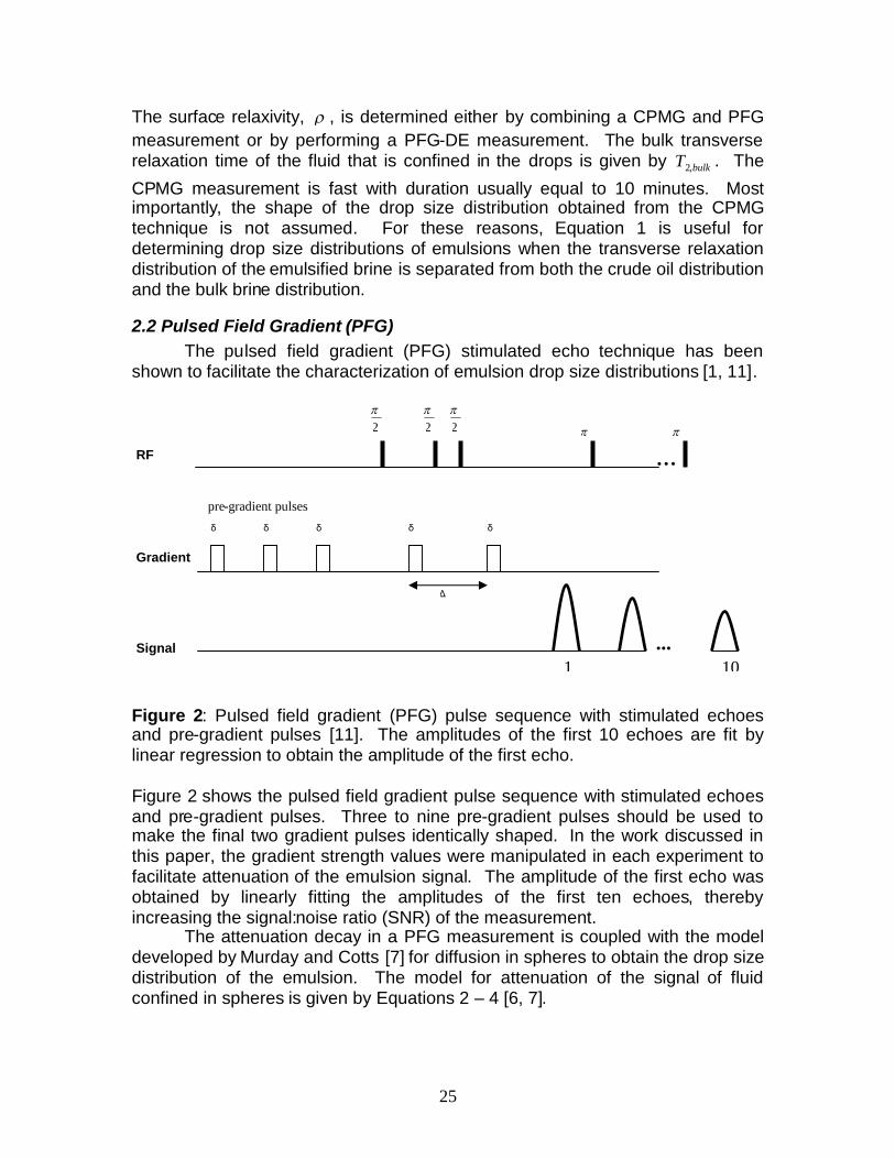
2.2 Pulsed Field Gradient (PFG)The pulsed field gradient (PFG) stimulated echo technique has been
shown to facilitate the characterization of emulsion drop size distributions [1, 11].
Figure 2: Pulsed field gradient (PFG) pulse sequence with stimulated echoesand pre-gradient pulses [11]. The amplitudes of the first 10 echoes are fit bylinear regression to obtain the amplitude of the first echo.
Figure 2 shows the pulsed field gradient pulse sequence with stimulated echoesand pre-gradient pulses. Three to nine pre-gradient pulses should be used tomake the final two gradient pulses identically shaped. In the work discussed inthis paper, the gradient strength values were manipulated in each experiment tofacilitate attenuation of the emulsion signal. The amplitude of the first echo wasobtained by linearly fitting the amplitudes of the first ten echoes, therebyincreasing the signal:noise ratio (SNR) of the measurement.
The attenuation decay in a PFG measurement is coupled with the modeldeveloped by Murday and Cotts [7] for diffusion in spheres to obtain the drop sizedistribution of the emulsion. The model for attenuation of the signal of fluidconfined in spheres is given by Equations 2 – 4 [6, 7].
Δ
2
RF
Signal
Gradient
δ δ δ
2
δ δ
2
1 10
...
pre-gradient pulses
…

26
1222222
22
)(2
)2(1
2expm DPmDPmmm
gsp DDrgR
(2)
))((exp)(exp2)(exp2))((exp2 2222 DPmDPmDPmDPm DDDD (3)The gyromagnetic ratio is given by g , the gradient strength is g , DPD is thediffusivity of the fluid in the dispersed phase, r is the radius of the emulsiondroplet, is the time between gradient pulses, is the gradient pulse duration,and m is the mth positive root of Equation 4.
)()(1
25
23 rJrJ
r
(4)
Jk is the Bessel function of the first kind with order k. The overall attenuation ofthe emulsion has been shown to be a function of the attenuation of both thecontinuous and dispersed phases [8].
0.10;)1( CPDPemul RRR (5)The fraction of the attenuation from the continuous phase is given by theparameter, .
1
,2
,2
exp)(
exp)(
1
CPiCPi
DPiDPi
Tf
Tf
(6)
The attenuation of the continuous phase, CPR , is expressed as the bulkattenuation of the continuous phase.
3exp 222
CPCP DgR (7)
The attenuation of the dispersed phase, DPR , is given by Equation 8 [5].
0
0)(
)(
)(
drrp
drRrpR
rsp
DP (8)
The volume weighted drop size distribution , )(rp , is the lognormal probabilitydensity function [1].
2
2
21 2
ln2lnexp
)2(2
1)(
vdr
rrp (9)
The volume based mean is given by vd and the width of the distribution is .The PFG technique involves obtaining attenuation of the signal as a
function of gradient strength and subsequently fitting the attenuation to thepredicted attenuation according to the restricted diffusion model. For this work, a
27
nonlinear least squares algorithm with optimization in MatLab was used toperform the fitting.
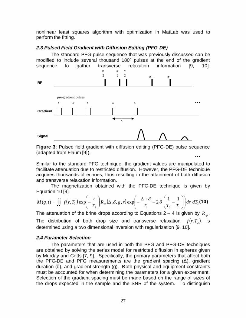
2.3 Pulsed Field Gradient with Diffusion Editing (PFG-DE)The standard PFG pulse sequence that was previously discussed can be
modified to include several thousand 180º pulses at the end of the gradientsequence to gather transverse relaxation information [9, 10].
Figure 3: Pulsed field gradient with diffusion editing (PFG-DE) pulse sequence(adapted from Flaum [9]).
Similar to the standard PFG technique, the gradient values are manipulated tofacilitate attenuation due to restricted diffusion. However, the PFG-DE techniqueacquires thousands of echoes, thus resulting in the attainment of both diffusionand transverse relaxation information.
The magnetization obtained with the PFG-DE technique is given byEquation 10 [9].
21212
211
2exp,,,exp,),( dTdrTTT
rgRTt
TrftgM sp
(10)
The attenuation of the brine drops according to Equations 2 – 4 is given by spR .
The distribution of both drop size and transverse relaxation, 2,Trf , isdetermined using a two dimensional inversion with regularization [9, 10].
2.4 Parameter SelectionThe parameters that are used in both the PFG and PFG-DE techniques
are obtained by solving the series model for restricted diffusion in spheres givenby Murday and Cotts [7, 9]. Specifically, the primary parameters that affect boththe PFG-DE and PFG measurements are the gradient spacing (Δ), gradient duration (δ), and gradient strength (g). Both physical and equipment constraintsmust be accounted for when determining the parameters for a given experiment.Selection of the gradient spacing must be made based on the range of sizes ofthe drops expected in the sample and the SNR of the system. To distinguish
Δ
2
RF
Signal
Gradient
δ δ δ
2
δ δ
2
pre-gradient pulses…
…

28
restricted diffusion from free diffusion, the dimensionless diffusion time must begreater than or equal to 1.0 [9].
0.12
2
rD
(11)
If Δ is too small, the measurement will not be sensitive to large drops. If Δ is too large, the SNR will be low.
2
2
3.02
TD
r (12)
After Δis established, the gradient duration, δ, is calculated. The minimum valueof the gradient duration is instrument specific, and the maximum value is basedon an established rule of thumb [9].
2.0min (13)With the gradient spacing and duration calculated, the gradient values whichachieve the desired attenuation can be calculated using the previously describedseries model for restricted diffusion in spheres. Ideally, for a given sphere size,the attenuation should range from 0.99 to 0.01 [9].
Figure 4 illustrates the relationship between the parameters in a givenexperiment.
Figure 4: Example of parameters calculated for PFG-DE and PFGmeasurements. These parameters were calculated with (ρ = 0.5 µm/s, Dbrine =2.45 x 10⁻⁹ m2/s, T2,bulk = 2.48 s, and Δ/T2 = 0.3).
In the top figure, the solid curve shows the T2 distribution of the dispersed fluid.The dashed curve is the gradient spacing, Δ, and the dotted curve is the gradientduration, δ. The minimum gradient spacing, Δmin, is shown as the dashed-dottedline in the top figure, as determined by the lower constraint on Δ. When thecalculated Δ falls below Δmin, the measurement is no longer sensitive to restricteddiffusion, thus resulting in the maximum drop size, rmax. The minimum detectable

29
drop size, rmin, is calculated based on the maximum gradient duration andmaximum gradient strength of the instrument. Finally, the bottom figure containsthe range of gradient values that should be used to facilitate the desired amountof attenuation ranging from 1% signal remaining, g01, to 99% signal remaining,g99. In this work, 25 logarithmically spaced gradient values were calculated foreach parameter set. For all PFG and PFG-DE measurements discussed in thispaper, 32 scans were used with the echo spacing equal to 600 µs and therelaxation delay equal to 10 s.
Using a technique developed by Flaum [9], multiple sets of parameterscan be used to characterize the entire drop size range (rmin – rmax). Thistechnique, referred to as masking, incorporates multiple parameter sets witheach set consisting of one Δ value, one δ value, and a logarithmically spaced list of gradient strength values. After the data have been collected, the results fromeach set are combined to obtain information about the entire drop size range.The sensitivity of each parameter set is limited by the SNR of the instrument.The masking technique applies to both drop size information and transverserelaxation information. The masking technique weights the most sensitive dropsize ranges of each parameter set based on the SNR of the measurement togain the most accurate information about the range of drop sizes. Similarly, thetransverse relaxation information is masked according to the gradient spacing. Inthis work, transverse relaxation times shorter than half of the gradient spacingwere truncated. If the emulsion is known to be unimodal, only one experimentalset of parameters needs to be used. However, if the drop size distribution of theemulsion is broad or multi-modal, multiple parameter sets should be employed tocharacterize the entire drop size range.
2.6 Emulsion PreparationThe emulsions considered in this work were prepared using a Couette
flow device. The rotating, inner cylinder was composed of Torlon with radius, rT= 19.1 mm. The stationary, outer cylinder was composed of glass with radius, rg
= 21.6 mm.
Figure 5: Cross section of the Couette flow device. Note that rT/rg = 0.88.
The rotational speed of the inner cylinder was adjusted depending on the desiredexperimental conditions, and the shear rate is given by Equation 14.
Tg
T
rrr
2(14)
The rotational speed of the inner cylinder is given by ω. The temperature of allmeasurements was maintained at 30º C. For all of the emulsions discussed, thedispersed phase was ASTM certified synthetic seawater, and the emulsions were
rg
rT

30
classified as water/oil. Two different oils were used for the continuous phase,denoted as either Crude Oil A or Crude Oil B.
3. ResultsThe following sections contain three different cases that show the
usefulness of the PFG-DE technique. The first case illustrates a situation whenthe T2 distribution of the emulsified brine overlaps the bulk brine T2 distribution.The second case illustrates the situation when the T2 distribution of theemulsified brine overlaps the T2 distribution of the crude oil. Finally, the thirdcase illustrates the ability of the PFG-DE technique to resolve a bimodal dropsize distribution.
3.1 Emulsified Brine T2 Distribution Overlaps the Bulk Brine T2 DistributionDrop size distributions of brine/Crude Oil A emulsions were obtained using
the CPMG, PFG-DE, and PFG techniques. Figure 6 shows the T2 distribution ofan emulsion that was formed by combining 10 mL of brine with 40 mL of CrudeOil A with viscosity equal to 15 cP. Shear was applied to the emulsion with γ = 1.3 x 10³ s-1 for 10 minutes.
Figure 6: T2 distribution of an emulsion with γ = 1.3 x 10³ s-1 for 10 minutes.Note the proximity of the emulsified brine T2 distribution to the bulk brine T2distribution.
Figure 6 shows the overlap of the emulsified brine T2 distribution and the bulkbrine T2 distribution. Figure 7 shows the drop size distribution that was obtainedby using the emulsified brine T2 distribution in conjunction with Equation 1.
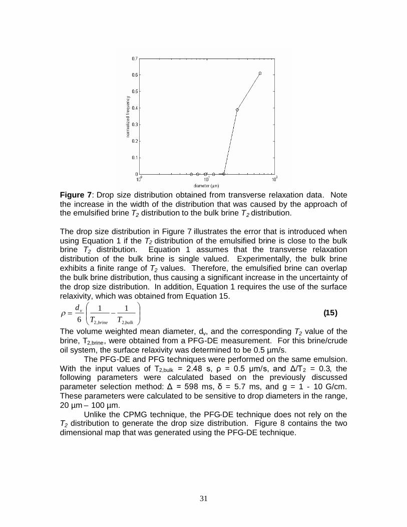
31
Figure 7: Drop size distribution obtained from transverse relaxation data. Notethe increase in the width of the distribution that was caused by the approach ofthe emulsified brine T2 distribution to the bulk brine T2 distribution.
The drop size distribution in Figure 7 illustrates the error that is introduced whenusing Equation 1 if the T2 distribution of the emulsified brine is close to the bulkbrine T2 distribution. Equation 1 assumes that the transverse relaxationdistribution of the bulk brine is single valued. Experimentally, the bulk brineexhibits a finite range of T2 values. Therefore, the emulsified brine can overlapthe bulk brine distribution, thus causing a significant increase in the uncertainty ofthe drop size distribution. In addition, Equation 1 requires the use of the surfacerelaxivity, which was obtained from Equation 15.
bulkbrine
v
TTd
,2,2
116
(15)
The volume weighted mean diameter, dv, and the corresponding T2 value of thebrine, T2,brine, were obtained from a PFG-DE measurement. For this brine/crudeoil system, the surface relaxivity was determined to be 0.5 µm/s.
The PFG-DE and PFG techniques were performed on the same emulsion.With the input values of T2,bulk = 2.48 s, ρ = 0.5 µm/s, and Δ/T2 = 0.3, thefollowing parameters were calculated based on the previously discussedparameter selection method: Δ = 598 ms, δ= 5.7 ms, and g = 1 - 10 G/cm.These parameters were calculated to be sensitive to drop diameters in the range,20 µm – 100 µm.
Unlike the CPMG technique, the PFG-DE technique does not rely on theT2 distribution to generate the drop size distribution. Figure 8 contains the twodimensional map that was generated using the PFG-DE technique.
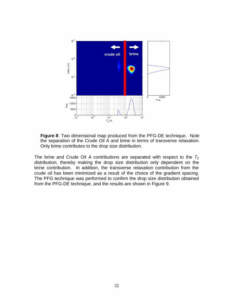
ThdibrcrThfro
crude oil brine
Figure 8: Two dimensional map produced from the PFG-DE technique. Notethe separation of the Crude Oil A and brine in terms of transverse relaxation.
32
e brine and Crude Oil A contributions are separated with respect to the T2stribution, thereby making the drop size distribution only dependent on theine contribution. In addition, the transverse relaxation contribution from theude oil has been minimized as a result of the choice of the gradient spacing.e PFG technique was performed to confirm the drop size distribution obtainedm the PFG-DE technique, and the results are shown in Figure 9.
Only brine contributes to the drop size distribution.

33
Figure 9: Comparison of drop size distributions obtained from the PFG-DE andPFG techniques. The drop size distribution from the PFG-DE technique given bythe mean and one standard deviation on either side of the mean [45, 59, 72] µmagrees well with the traditional PFG technique, [47, 58, 72] µm.
Because the PFG-DE technique yields a discrete drop size distribution and thePFG technique yields a continuous probability density function, a relationshipmust be established between the results of the two techniques. The cumulativedistribution can be written according to Equation 16.
ij
jjfdP
1
(16)
The normalized frequency obtained from the PFG-DE technique is given by fj.Because the probability density function is lognormal with equal increments ofthe logarithm of the diameter, the cumulative distribution can further be written interms of the normalized frequency from the PFG-DE technique.
iiiii fddpdP log (17)The probability density function is denoted by p(di). Thus, the results from bothtechniques can be accurately plotted on the same figure. Figure 9 reveals theagreement between the PFG-DE and PFG techniques for the drop sizedistribution of this emulsion. Unlike the CPMG technique as shown in Figure 7,the PFG-DE and PFG techniques have the ability to resolve the drop sizedistribution when the T2 distribution of the emulsion overlaps the bulk brine T2distribution. Table 1 contains a summary of this comparison.
Table 1: Summary of results for the brine/Crude Oil A emulsion with γ = 1.3 x 10³ s-1.
Method ed v (µm)
vd (µm) edv (µm)
PFG-DE 45 59 72
PFG 47 58 72

34
3.2 Emulsified Brine T2 Distribution Overlaps the Bulk Crude Oil T2Distribution
If the T2 distribution of the emulsified brine overlaps the T2 distribution ofthe crude oil in the emulsion, the transverse relaxation data cannot be used toobtain the drop size distribution of the emulsion. An emulsion was prepared bycombining 5 mL of brine with 20 mL of Crude Oil B with viscosity equal to 1 cP.The emulsion was sheared for five minutes with γ = 3.2 x 10³ s-1. Figure 10contains the T2 distribution of the emulsion showing the overlap of the emulsifiedbrine and crude oil T2 distributions.
Figure 10: Overlap of emulsion and Crude Oil B T2 distributions.
The solid curve in Figure 10 is the T2 distribution of the layered Crude Oil B/brinesample, and the dashed curve is the T2 distribution of the emulsion. Because theemulsified brine and Crude Oil B T2 distributions are not separable, Equation 1cannot be used to calculate the drop size distribution.
The parameters for the PFG-DE technique were calculated based on(T2,bulk = 2.48 s, ρ = 0.3 µm/s, and Δ/T2 = 0.3), and the values were: Δ = 552 ms,δ= 28 ms, and g = 1 – 13 G/cm. The parameters were sensitive to dropdiameters in the range, 5 – 50 µm. The two dimensional map obtained from thePFG-DE technique is shown in Figure 11.

35
Figure 11: Two dimensional map of brine/Crude Oil B emulsion. The emulsifiedbrine and Crude Oil B T2 distributions overlap, but the Crude Oil B does notcontribute to the drop size distribution because the Crude Oil B signal attenuatedsignificantly.
Figure 11 shows that the drop size distribution of the brine phase was extractedusing the PFG-DE technique even though the T2 distributions of the emulsifiedbrine and Crude Oil B overlap. The lack of contribution of the Crude Oil B to thedrop size distribution is evident when considering the attenuation of the emulsionas shown in Figure 12.

36
Figure 12: Experimental and predicted attenuation for the brine/Crude Oil Bemulsion (Δ = 552 ms, δ = 28 ms, and g = 1 – 13 G/cm). Note that the Crude OilB does not contribute to the attenuation of the signal of the emulsion, therebyfacilitating the separation of the Crude Oil B and brine contributions.
Figure 12 shows that the Crude Oil B does not significantly contribute to theattenuation of the signal of the emulsion based on Equation 7. The signal of theCrude Oil B is negligible after the second gradient pulse; therefore, the brine andCrude Oil B contributions can be separated.
The PFG measurement was performed using the same parameters asthose used for the PFG-DE measurement, and the comparison of the drop sizedistributions is shown in Figure 13.
Crude Oil B BulkAttenuation

Figure 13: Comparison of drop size distributions obtained from the PFG-DE andPFG techniques. The drop size distribution from the PFG-DE technique, [14, 19,24] µm, agrees well with the traditional PFG technique [14, 21, 31] µm.
Figure 13 shows that the means of the drop size distributions are in agreementfor the two techniques, while the widths of the distributions are slightly different.The difference in the widths of the distributions is likely caused by theassumption of the PFG technique that the drop size distribution is lognormal.The PFG-DE technique is not restricted by the assumption that the drop sizedistribution is lognormal. Table 2 contains a summary of the results for thisbrine/Crude Oil B emulsion.
Table 2: Summary of results for the brine/Crude Oil B emulsion with γ = 3.2 x 10³ s-1.
Method ed v (µm)
vd (µm) ed v (µm)
PFG-DE 14 19 24
37
3.3 Bimodal Drop Size DistributionThe PFG-DE technique is particularly useful for determining the drop size
distribution when the emulsion contains a bimodal drop size distribution. Abimodal drop size distribution was prepared by combining two independentlyformed emulsions. One emulsion was prepared by shearing 10 mL of brine with40 mL of Crude Oil A. The shearing duration was 10 minutes with γ = 2.3x10³ s-
1. An independent emulsion consisting of 10 mL of brine and 40 mL of Crude OilA was formed with γ = 1.3x10³ s-1 and duration equal to 10 minutes. The PFG-
PFG 14 21 31

38
DE and PFG measurements were performed on both of the independentemulsions. From each independent emulsion, 25 mL was removed andcombined into one glass sample vessel to form a bimodal drop size distribution.The PFG-DE measurement was performed on the combined emulsion.
By applying two different shear rates, it was expected that two differentpopulations of drops would form. Therefore, two different parameter sets wereconstructed to characterize the two different drop size distributions. With γ = 2.3x10³ s-1, the expected range of drop diameters was 5 – 50 µm. Tocharacterize this range of diameters, the following parameters were calculatedusing the previously described algorithm based on T2,bulk = 2.48 s, ρ = 0.5 µm/s, and Δ/T2 = 0.3: Δ = 470 ms, δ= 28 ms, g = 1 – 21 G/cm. The PFG techniquewas also used to measure the drop size distribution of the emulsion, and thecomparison is shown in Figure 14.
Figure 14: Comparison of drop size distributions with γ = 2.3 x 10³ s-1. The PFG-DE technique yielded a drop size distribution, [10, 15, 20] µm, that agreed withthe PFG technique, [11, 15, 19] µm.
Figure 14 shows the agreement that was achieved between the PFG-DEtechnique and the PFG technique with γ = 2.3x10³ s-1.
With γ = 1.3x10³ s-1, the expected range of drop diameters was 30 – 100µm. To characterize this range of diameters, the following parameters werecalculated using the previously described algorithm based on T2,bulk = 2.48 s, ρ = 0.5 µm/s, and Δ/T2 = 0.3: Δ = 598 ms, δ = 5.7 ms, g = 1 – 19 G/cm. The PFGtechnique was also used to measure the drop size distribution of the emulsion,and the comparison is shown in Figure 15.

39
Figure 15: Comparison of drop size distributions with γ = 1.3 x 10³ s-1. The PFG-DE technique yielded a drop size distribution, [42, 60, 78] µm, that agreed withthe PFG technique, [50, 66, 87] µm.
Figure 15 shows the agreement that was achieved between the PFG-DE andPFG techniques with γ = 1.3x10³ s-1.
An emulsion with a bimodal drop size distribution was formed bycombining 25 mL of the emulsion with γ = 2.3 x 10³ s-1, with 25 mL of theemulsion with γ = 1.3 x 10³ s-1. The PFG-DE measurement of the bimodalemulsion consisted of two complete parameter sets: [Δ = 470 ms, δ = 28 ms, g = 1 – 21 G/cm] and [Δ = 598 ms, δ = 5.7 ms, g = 1 – 19 G/cm]. The maskingtechnique developed by Flaum [9] was used to investigate the range of sizes ofthe bimodal distribution. The sensitivity of each parameter set is determined bythe amount of noise in the measurement. Figure 16 illustrates the determinationof the sensitive region of each parameter set by plotting the sum of the square ofthe difference in attenuation for different drop sizes as a function of drop size.

40
The horizontal line in Figure 16 was calculated using Equation 18 [9]. gradnoise Ncutoff 22 (18)
In this equation, the standard deviation of the noise is given by σnoise and thenumber of gradients is given by Ngrad. For this example, the value of the cutoffwas calculated to be 0.02, as illustrated in Figure 16. The intersections of thehorizontal line with the sensitivity curves designate the boundaries of thesensitivity of each parameter set. For example, the first parameter set, shown asthe solid curve, is sensitive to drop diameters in the range, 5 µm – 70 µm. Thefirst parameter set yielded the results shown in Figure 17.
Figure 16: Sensitivity of the two parameter sets.

41
Figure 17: Two dimensional results from the first parameter set. The mostsensitive drop size is indicated by the solid line while the limits of the sensitivity ofthe measurement are indicated by the dashed lines. Note that the population ofsmaller drops exists in the sensitive region.
Figure 17 shows the sensitive region obtained by using the first parameter set.The solid line indicates the drop size that the measurement is most sensitive to,and the dashed lines indicate the limits of the sensitivity of the measurement asgiven by Equation 18. Similarly, the second parameter set was performed on theemulsion to yield the results shown in Figure 18.
Figure 18: Two dimensional results from the second parameter set. Note thatthe larger population of drop sizes is present in the sensitive region.
The second parameter set is clearly sensitive to the larger population of dropsizes as shown in Figure 18.

42
In addition to masking the measurement according to the drop size, themasking procedure also truncates the transverse relaxation based on thegradient spacing, Δ, of the measurement. As mentioned in Section 2.4, alltransverse relaxation times that are less than half of Δ are truncated. For thismeasurement, the limit for transverse relaxation times was set to 235 ms whichwas half of the shortest Δ, 470 ms. For this example, truncating the transverserelaxation merely diminishes the transverse relaxation contribution of the crudeoil while the brine contribution is unaffected. Figure 19 shows the final resultafter masking both transverse relaxation and drop size.
The Crude Oil A and brine contributions were isolated according to theseparation in terms of the T2 distributions, and the resulting bimodal drop sizedistribution is given in Figure 20.
Figure 19: Two dimensional map of the bimodal drop size distribution aftermasking. The brine contribution to the drop size distribution was isolatedaccording to the separation of the T2 distributions.

43
Figure 20: Comparison of unimodal drop size distributions with the bimodal dropsize distribution obtained using the PFG-DE technique.
Figure 20 illustrates the ability of the PFG-DE technique to resolve the bimodaldrop size distribution. The independently measured unimodal drop sizedistributions of each emulsion are plotted in conjunction with the bimodal dropsize distribution. Figure 20 shows that the first population of sizes in the bimodaldistribution, [11, 14, 17] µm, agrees with the PFG-DE measurement of thecorresponding unimodal drop size distribution, [10, 15, 20] µm. In addition, thesecond population of drop sizes in the bimodal distribution, [39, 52, 65] µm, alsoagrees with the PFG-DE measurement of the corresponding unimodaldistribution, [42, 60, 78] µm. These results show that the PFG-DE technique hasthe ability to resolve a bimodal drop size distribution which is in agreement withthe independent, unimodal drop size distributions.
4. ConclusionBased on the work presented in this paper, the PFG-DE technique has the
ability to resolve drop size distributions of emulsions in different physicalsituations. In addition, the parameter selection algorithm developed by Flaum [9]facilitates accurate measurements of drop size distributions of emulsions. Theresults from the PFG-DE technique have been shown to agree with the traditionalPFG technique for lognormal drop size distributions. The PFG-DE techniquealso has the ability to resolve more complicated drop size distributions such asbimodal drop size distributions. In general, the PFG-DE technique is usefulbecause it provides both transverse relaxation and drop size distributionssimultaneously, and it is not constrained by an assumed shape of the drop sizedistribution.
44
Acknowledgements
The authors would like to thank Dick Chronister, Waylon House, Dr.Alberto Montesi, Dr. Jeff Creek, Mike Rauschhuber, and Chevron for financialsupport.
References1. Pena, A. and G.J. Hirasaki, NMR Characterization of Emulsions, in
Emulsions and Emulsion Stability, J. Sjoblom, Editor. 2006, CRC: BocaRaton, FL.
2. Becher, P., Emulsions: Theory and Practice. 2001, New York: OxfordUniversity Press.
3. Schramm, L.L., Emulsions, Foams, and Suspensions: Fundamentals andApplications. 2005: Wiley-VCH.
4. Sjoblom, J., Encyclopedic Handbook of Emulsion Technology. 2001, NewYork: Marcel Dekker.
5. Packer, K.J. and C. Rees, Pulsed NMR Studies of Restricted Diffusion I.Droplet Size Distributions in Emulsions. Journal of Colloid and InterfaceScience, 1972. 40(2).
6. Neuman, C.H., Spin Echo of Spins Diffusing in a Bounded Medium.Journal of Chemical Physics, 1974. 60: p. 4508-4511.
7. Murday, J.S. and R.M. Cotts, Self-Diffusion Coefficient of Liquid Lithium.Journal of Chemical Physics, 1968. 48: p. 4938-4945.
8. Pena, A., Enhanced Characterization of Oilfield Emulsions via NMRDiffusion and Transverse Relaxation Experiments. Advances in Colloidand Interface Science, 2003. 105: p. 103-150.
9. Flaum, M., Fluid and Rock Characterization Using New NMR Diffusion-Editing Pulse Sequences and Two Dimensional Diffusivity-T2 Maps, inChemical and Biomolecular Engineering. 2006, Rice University: Houston.
10. Hurlimann, M.D. and L. Venkataramanan, Quantitative Measurement ofTwo Dimensional Distribution Functions of Diffusion and Relaxation inGrossly Inhomogeneous Fields. Journal of Magnetic Resonance, 2002.157: p. 31-42.
11. Garisanin, T. and T. Cosgrove, NMR Self-Diffusion Studies on PDMS Oil-in-Water Emulsion. Langmuir, 2002. 18: p. 10298-10304.
12. Carr, H.Y. and E.M. Purcell, Effects of Diffusion on Free Precession inNuclear Magnetic Resonance Experiments. Physical Review, 1954. 94: p.630-638.
13. Meiboom, S. and D. Gill, Modified Spin-Echo Method for MeasuringNuclear Relaxation Times. The Review of Scientific Instruments, 1958. 29:p. 688-691.

45
Task 2. Estimation of fluid and rock properties and their interactions fromNMR relaxation and diffusion measurements
Subtask 2.4 Interpretation of systems with diffusional couplingbetween pores
NMR DIFFUSIONAL COUPLING:EFFECTS OF TEMPERATURE AND CLAY DISTRIBUTION
Vivek Anand, George J. Hirasaki, Rice University, USA
Marc Fleury, IFP, France
ABSTRACTThe interpretation of Nuclear Magnetic Resonance (NMR) measurements on fluid-saturated formations assumes that pores of each size relax independently of otherpores. However, diffusional coupling between pores of different sizes may lead tofalse interpretation of measurements and thereby, a wrong estimation of formationproperties. The objective of this study is to provide a quantitative framework for theinterpretation of the effects of temperature and clay distribution on NMRexperiments. In a previous work, we established that the extent of couplingbetween a micropore and macropore can be quantified with the help of a couplingparameter () which is defined as the ratio of characteristic relaxation rate to therate of diffusive mixing of magnetization between micro and macropore. The effectof temperature on pore coupling is evaluated by proposing a temperaturedependent functional relationship of . This relationship takes into account thetemperature dependence of surface relaxivity and fluid diffusivity. The solution ofinverse problem of determining and microporosity fraction for systems withunknown properties is obtainable from experimentally measurable quantities.
Experimental NMR measurements on reservoir carbonate rocks and modelgrainstone systems consisting of microporous silica gels of various grain sizes areperformed at different temperatures. As temperature is increased, the T2 spectrumfor water-saturated systems progressively changes from bimodal to unimodaldistribution. This enhanced pore coupling is caused by a combined effect ofincrease in water diffusivity and decrease in surface-relaxivity with temperature.Extent of coupling at each temperature can be quantified by the values of . Thetechnique can prove useful in interpreting log data for high temperature reservoirs.

46
Effect of clay distribution on pore coupling is studied for model shaly sands madewith fine silica sand and bentonite or kaolinite clays. The NMR response ismeasured for two cases in which clay is either present as a separate, discretelayer or homogeneously distributed with the sand. For layered systems, T2
spectrum shows separate peaks for clay and sand at 100% water saturation and asharp T2,cutoff could be effectively applied for estimation of irreducible saturation.However, for dispersed systems a unimodal T2 spectrum is observed andapplication of 33ms T2,cutoff would underestimate the irreducible saturation in thecase of kaolinite and overestimate in the case of bentonite. The inversiontechnique can still be applied to accurately estimate the irreducible saturation.
INTRODUCTIONNMR well logging provides a useful technique for the estimation of formationproperties such as porosity, permeability, irreducible water saturation, oilsaturation and viscosity. The conventional interpretation of NMR measurementson fluid-saturated rocks assumes that the relaxation rate of fluid in a pore isdirectly related to the surface-to-volume ratio of the pore. In addition, each pore isassumed to relax independently of other pores so that the relaxation timedistribution represents a signature of the distribution of pore sizes. Ramakrishan etal (1999) showed that such interpretation often fails if the fluid molecules in intra(micro) and intergranular (macro) pores are diffusionally coupled with each other.The pore coupling effects can be particularly enhanced at high formationtemperatures and a calibration for the estimation of irreducible saturations basedon laboratory data at room temperature may not be suitable.
In a previous work (Anand and Hirasaki, 2005), we demonstrated that the extent ofcoupling in a pore model consisting of a micropore in contact with a macroporecan be quantified with the help of a coupling parameter (). is defined as theratio of characteristic relaxation rate of the pore to the rate of diffusional mixing ofmagnetization between micro and macropore i.e.
2Characteristic relaxation rate 2Diffusion rate 1
LDL
(1)
where is the micropore surface relaxivity, is the microporosity fraction, L2 is thehalf length of the macropore and L1 is the half width of the micropore (refer tofigure 1 in reference 2). Numerical simulations show that as decreases, couplingbetween micro and macropore increases and the T2 response of the pore changesfrom bimodal to unimodal distribution. The amplitude of the faster relaxing(micropore) peak,, shows an empirical lognormal relationship with .

47
log 2.291 1 erf2 0.89 2
(2)
The pore types can, thus, communicate through three coupling regimes: Totalcoupling (=0), Intermediate coupling (0<<) and Decoupled (=) regime. Forsystems with unknown physical and geometrical properties, the solution of inverseproblem of determining and can be obtained from intersection of contours ofconstant and T2,macro/T2, in and parameter space (Figure 17 in reference2). Here T2,macro and T2,are the modes of the macropore and micropore peaks at100% water and irreducible saturation respectively. The model was experimentallyvalidated for pore coupling in several grainstones systems and clay lining pores insandstones.
The purpose of this paper is to extend the earlier work to describe the effect oftemperature and clay distribution on pore coupling. In the first section, atemperature dependent functional relationship of is proposed by incorporatingthe temperature variation of surface relaxivity and fluid diffusion-coefficient. NMRmeasurements are performed at various temperatures with series of modelgrainstone systems and reservoir carbonate core at irreducible and 100% watersaturation. Measurements at irreducible water saturation show that surfacerelaxivities for both systems decrease with temperature. The results for 100%water saturated systems illustrate that as temperature is increased, T2 distributionsgradually transition from bimodal to unimodal spectra suggesting an increase inpore coupling with temperature. Estimation of theoretically predicts the transitionof the systems between coupling regimes as temperature is increased. In thesecond section, diffusional coupling between free and irreducible water in shalysands is studied as a function of distribution of clays with the sand. Model shalysands are prepared in two ways such that the clays are either homogenouslydispersed with sand or present as a separate, discrete layer. NMR measurementsat 100% and irreducible water saturation show that the free and irreducible watercan be diffusionally coupled or decoupled depending on the spatial separationbetween them.
EFFECT OF TEMPERATURE ON DIFFUSIONAL COUPLINGRelaxation rates of bulk fluids are strongly temperature sensitive due to thethermal modulation of translational and rotational correlation times. For fluids inporous media, relaxation is usually dominated by surface relaxation which can betemperature dependent. In addition, diffusional coupling between pores of differentsizes can also increase with temperature due to increased diffusional transport offluid molecules. Thus, the interpretation of temperature effect on NMRmeasurements in porous media needs to take into account the temperaturevariation of both surface relaxation and diffusional coupling.

48
The effect of temperature on pore coupling can be quantified by incorporating thetemperature dependencies of surface relaxivity and diffusion coefficient in thefunctional relationship for . Surface relaxation of fluid molecules in porous mediais governed by two processes (Godefroy et al, 2001). First, translational motion ofthe fluid molecules near the paramagnetic sites at pore surface and second,exchange between surface and bulk molecules. The temperature dependence ofsurface relaxation arises from the thermal activation of the translational motion atthe pore surface as well as increased exchange between surface and bulk fluidmolecules. Quantitatively, the temperature dependence can be expressed as anArrhenius relationship
0 exp ERT
(3)
where E is the effective activation energy and R is the universal gas constant.Self-diffusion of bulk fluids is also a thermally activated process and the diffusioncoefficient usually shows Arrhenius dependence with temperature,
o exp aED DRT
(4)
In the above equation, Ea is the activation energy for the diffusion process and Do
is the diffusion coefficient at infinite temperature. Substituting equations (3) and (4)in the expression for α (equation 1) and grouping variables, a temperaturedependent functional relationship of αcan be given as
oo
1 1exp aE ER T T
(5)
where αo is the value of coupling parameter at reference temperature To. Thus,pore coupling can either increase or decrease with temperature if the difference inthe activation energy for diffusion and relaxation process (Ea+E) is positive ornegative, respectively.
Experimental Validation
The effect of temperature on NMR diffusional coupling is experimentally studied fortwo systems of porous media. The first system consists of a homologous series ofmicroporous silica gels with varying grain diameters. The second system consistsof a reservoir carbonate core with bimodal pore size distribution. For both systemsNMR measurements are performed at total and irreducible water saturation as afunction of temperature.
49
Silica Gels
Silica gels with mean grain radii of 118m (Medium Coarse), 55m (Very Fine)and 28m (Silt size) were obtained from Sigma Aldrich. The physical properties ofthe gels are given in Table 2 of reference 2. Figure 1 shows the T2 distributions at100% water saturation for the three silica gels at 30, 50, 75 and 95oC. At eachtemperature, the distributions are normalized with the pore volume (area under thecurve) to account for the Curie Law. Figure 2 shows the normalized T2distributions at irreducible condition for the medium coarse silica gel at the abovementioned temperatures. The NMR apparatus has a response around 1 ms at hightemperatures which has been subtracted from the distributions.
The increase in relaxation time at irreducible condition with temperature (Figure 2)shows that the surface relaxivity decreases as the temperature is increased. Thisresult is in agreement with those obtained by Ramakrishnan et al (1999) who sawa similar increase in the relaxation time of water-saturated systems withtemperature. The temperature behavior at 100% water saturation can now beinterpreted keeping in mind the negative dependence of relaxivity on temperature.Each of the three silica gels in Figure 1 represents a different coupling scenario.The medium coarse silica gel is almost in decoupled regime (/= 0.97) at 30oC.As the temperature is increased, surface relaxivity decreases and diffusivity ofwater increases. As a result, coupling between micro and macropores increasesand the system transitions from almost decoupled to intermediate coupling regime.This is evidenced by the reduction in the amplitude of the micropore peak anddecrease in the relaxation time of the macropore with temperature. Very fine silicagel is in intermediate coupling regime at 30oC (/= 0.24). Increasing thetemperature increases coupling so that the T2 distribution changes from bimodal at30oC to unimodal at higher temperatures. However, the increase in relaxation rateof the macropore due to coupling is exactly cancelled by the decrease in surfacerelaxation and thus the position of macropore peak remains unchanged. Silt sizesilica gel has a unimodal T2 distribution at 30oC suggesting that the system is intotal coupling regime (/~ 0). Increase in temperature has no further effect oncoupling but the corresponding decrease in surface relaxivity leads to a shift of T2
distribution to longer relaxation times. The results demonstrate that temperaturecan have apparently different effects on the NMR response even though thesystems may be governed by similar principles.
Reservoir Carbonate Core
The carbonate core studied is a Thamama reservoir carbonate with porosity 21.2%and water permeability of 13mD. Analysis of lithology shows that the carbonate isa packstone/wackestone with mainly moldic macroporosity in leached areas. Themicroporosity is predominantly inside pellets and mud. Figure 3 shows the T2
50
distributions of the core at 100% and irreducible water saturation (oil saturated) forthree temperatures of 25, 50 and 80oC. We can see that for 100% water-saturatedcore, as the temperature is increased amplitude of the micropore peak andrelaxation time of the macropore decrease. This suggests that diffusional couplingbetween micro and macropores is increasing with temperature. Similar to the casefor silica gels, the increase in pore coupling is due to increase in water diffusivityas well as decrease in surface relaxivity with temperature. The latter claim isbased on the fact that the relaxation time of the residual water in the micropores ofoil saturated core increases with temperature (lower panel of figure 3). Animportant implication of the results is that application of a sharp T2,cutoff based on alaboratory calibration at room temperature for the estimation of irreduciblesaturation may not be suitable for high temperature formations.
Discussion
Effect of temperature on pore coupling for the two systems can be analyzedquantitatively from the temperature variation of . For silica gels, at differenttemperatures can be calculated by including the temperature dependence ofsurface relaxivity and diffusivity in the definition of for grainstone systems (Anandand Hirasaki, 2005),
2
grain
( )( )
( )gT R
TD T R
(6)
Here Rg is the grain radius and R is the micropore radius (75 Å for silica gels).The temperature variation of surface relaxivity is obtained from measurements atirreducible saturation (Figure 2). The estimates of self-diffusion coefficient of wateras a function of temperature are obtained from the experimental data of Holz et al(2000). For the carbonate core, is calculated using the inversion techniquedescribed earlier. Figure 4 shows the cross plot of the normalized micropore-peakamplitude (/) with for the three silica gels and carbonate core. It can be seenthat accurately predicts the transition of the different coupling regimes withtemperature as the systems move downward along the empirical relationship(Equation 2). The microporosity fraction, estimated using the inversion technique,agrees within 5% average absolute deviation as shown in Figure 5. Thus, thetechnique can prove useful in accurately estimating formation properties forreservoirs at elevated temperatures.
EFFECT OF CLAY DISTRIBUTION ON PORE COUPLINGNMR well logging has evolved as a promising technology for the formationevaluation of shaly sands. Coates et al. (1994) proposed that the fast relaxingcomponents of the T2 spectrum in clayey rocks can be attributed to the wateradsorbed on clays. This idea was further extended by Prammer et al. (1996) who
51
found that clays in sandstones exhibited specific transverse relaxation timesproportional to their surface area and cation exchange capacity (CEC). Thus, theypostulated that the position of fast relaxing T2 peak can be used for clay typing.This claim was disputed by Matteson et al. (2000) who found that relaxation timeof clay brine slurries is a function of compaction of clays. Since the degree ofcompaction of formation clays is usually not known, they argued that clay typingfrom T2 measurements alone is not possible. In addition, they found that distinctpeaks for clay bound and free water were not visible for the clay-brine slurries.
In order to understand the phenomenological factors causing the apparentdifferences, a systematic study of the relaxation characteristics of clay-sandsystems was undertaken. Two systems of model shaly sands consisting of varyingamount of either kaolinite or bentonite clay and fine sand were prepared. In thefirst system, the clays were uniformly dispersed (dispersed systems) with the sandsuch that the clays occupied the interstitial voids between the sand grains. For thesecond system, clays were present as a separate, discrete layer with the sand(laminated systems). NMR response of the systems was measured at 100% andirreducible water saturations.
Experimental Section
Fine sand (grain radius 50m), kaolinite and bentonite clays were obtained fromSigma Aldrich. The physical properties of the materials are given in Table 1. Thedispersed and laminated systems were prepared in three sets such that the clay(either kaolinite or bentonite) constituted 0, 2, 5 and 10% of the total solid content.For each set, the systems were prepared at total and irreducible water saturationseparately. The details for the preparation of the systems are included below.
Dispersed System
To prepare the dispersed system at 100% water saturation, 15 grams of fine sandwas taken in a plastic centrifuge tube. The amount of either clay required to makethe desired weight percentage content was added to the sand and the mixture wasvigorously shaken to disperse the clay in the interstitial voids between the sandgrains. 5 ml of 0.1M calcium chloride solution was added to the mixture to makethick slurries. The slurries were mixed with a glass rod to further homogenize theclays with the sand and then compacted at a relative centrifugal force (RCF) of1500g. The small amount of supernatant water obtained after centrifuging wasremoved.
The dispersed systems at irreducible conditions were made by first preparing thewater saturated slurries in a 1’’ by 1’’ teflon sleeve. The base of the sleeve was

52
sealed with a covering of teflon tape. 15 grams of sand and desired amount ofeither clay were mixed in the sleeve and the mixture was saturated with 5 ml ofCaCl2 solution The slurries were then centrifuged in a Beckman rock corecentrifuge at an air/water capillary pressure of 50psi (which also approximatelycorresponds to 1500g RCF) for 3 hours to drain the free water. The teflon base ispermeable to water but prevents any grain loss during centrifugation.
Laminated System
15g of fine sand and 15ml calcium chloride solution were taken in a centrifugetube and
compacted at 1500g RCF for half hour. The required amount of either clay wasadded to the sand and centrifuged for 3 hours to compact the systems. Since thesand had already settled before the introduction of clay, there was no elutriation ofthe clay with sand. Clay, thus, compacted as a laminated layer on top of the sand.
Laminated systems at irreducible conditions were prepared analogously to thedispersed systems at irreducible condition. 15 grams of sand was allowed to settlegravimetrically in 15ml calcium chloride solution in a 1’’ by 1’’ sleeve with a sealedbase. The required amount of either clay was added to the sand and the systemswere centrifuged at 50psi air/brine capillary pressure to drain the free water.
Results and Discussion
Fig 6 and 7 show the T2 distributions of the dispersed and laminated kaolinitesystems at 100% water saturation. Figures 8 and 9 show the correspondingdistributions for the dispersed and laminated bentonite systems. For each case,the distributions at irreducible conditions are also shown for comparison. Analysisof the T2 distributions in figures 6-9 shows that the systems exhibit differentrelaxation characteristics when the clays are dispersed or layered with sand. Forthe dispersed systems, the T2 distributions at 100% water saturation showunimodal spectra. The laminated systems, on the other hand, show bimodal T2distributions at 100% water saturation. The fast and slow relaxing peaks in thebimodal distributions correspond to water in the clay and sand layer respectively.Note that the faster relaxation of water in bentonite (~4 ms) compared to that inkaolinite (~25ms) is due to the large interlayer surface area in swelling bentoniteclay. Bimodal T2 distributions for the laminated systems indicate that waterpopulations in the clay and sand layer are decoupled. On the other hand, unimodalT2 distributions for the dispersed systems indicate that water in the interstitialpores between clay and sand is diffusionally coupled. Figure 10 shows that therelaxation rate of water in dispersed systems shows a linear dependence with theclay content. Extrapolation of the linear relationship to zero clay fractions has an
53
intercept close to the relaxation rate of water in sand-only system. Thus, therelaxation rate of water in the dispersed systems can be expressed as
sand sand clay clay
2 total
1 S ST V
(7)
where sandSsand and claySclay are the products of relaxivity and surface area forsand and clay respectively and Vtotal is the total volume of water. Since therelaxation rate is simultaneously influenced by both clay and sand surface areas,we do not observe distinct peaks for irreducible and free water.
A quantitative estimate of characteristic lengths required for the systems to be incoupled or decoupled regime can be obtained from the analysis of for thesystems. For coupled systems, αis given as (Anand and Hirasaki, 2005)
active total22
S VD L
(8)
Since the surface area of the sand is negligible compared to that of the clays,relaxation at
the surface of the sand grains can be neglected in comparison to that on the claysurface
active clay clayS S (9)
For total coupling regime αis less than 1. Thus,
total2
clay clay
DVL
S (10)
for totally coupled regime. For decoupled regime αis greater than 50 (based on/= 0.97 in equation 2). Thus,
total2
clay clay
50DVL
S (11)
for decoupled regime. From the values of relaxivity and surface area of the clays(Table 1), we find that the characteristic diffusion length for total coupling regimeshould be less than 15m and 5m for kaolinite and bentonite respectively. Sincethese values are of the order of the interstitial pores between the sand grains withgrain radius of 50m, irreducible and free water in dispersed systems are coupledwith each other. For the decoupled regime, the diffusion length should be greaterthan 110m and 35m for kaolinite and bentonite respectively. Since theseparation between clay and sand layer is of the order of two centimeters in the

54
laminated systems, we observe distinct peaks for the irreducible clay water andfree water.
Estimation of Irreducible water saturation
Irreducible water for the sand-clay systems consists of both clay bound andcapillary bound water. The two populations are in close physical proximity andthus, relax at same rates due to fast diffusional exchange (Allen et al, 1998). If,however, the distance between the irreducible and free water is large, the twopopulations can relax independently with distinct relaxation times. This wasexperimentally demonstrated for the laminated systems which showed separatepeaks for clay and sand layers at 100% water saturation. Thus, for laminatedsystems a sharp cutoff is applicable to partition the T2 distributions into theirreducible and free water fractions. Note that in the model shaly sands consideredin this study, there will be an overestimation of irreducible water if a sharp T2,cutoff isapplied at the valley between clay and sand peak. This is due to the additionalcompaction of the clays during centrifugation as the water squeezes out of the claylayer.
The dispersed systems, on the other hand, are in coupled regime and theapplication of a sharp T2,cutoff to estimate the irreducible water would give wrongestimates. For example, application of conventional 33 ms cutoff wouldoverestimate the irreducible saturation in the case of bentonite and underestimatein the case of kaolinite particularly for cases with high clay content. The coupledresponse necessitates the application of inversion technique for accurateestimation of irreducible saturation. Since the systems are in total coupled regime,the irreducible saturation is given by the ratio of modes of relaxation time peaks atirreducible saturation and 100% water saturation (Anand and Hirasaki, 2005),
2,μ
2,macro 1
TT
(12)
Figure 11 shows the cross plot of the irreducible saturation obtained usingequation (12) with that obtained experimentally from NMR measurements atirreducible saturation. The estimates fall within 4% of the average absolutedeviation proving the applicability of the technique. The higher irreduciblesaturation for bentonite systems than for kaolinite is due to the presence ofinterlayer water.
These experiments also explain the apparent differences in the results reported byMatteson et al (2000) and Prammer et al (1996). The absence of peak at fastrelaxation time for the clay slurries which can be interpreted as clay bound water isdue to fast diffusional exchange between clay bound and free water. However,

55
when clays are present as laminated layers or as pore filling masses, theseparation between irreducible water and free water is large enough to decouplethe NMR responses. Thus, some sandstones can display distinct peaks for clayand free water with the clay response being proportional to the CEC of the clay, aswas indeed observed by Prammer et al (1996).
CONCLUSIONSNMR diffusional coupling between micro and macropores is studied for the effectsof temperature and clay distribution. The effect of temperature on pore coupling isquantified by incorporating the temperature dependence of surface relaxivity anddiffusion coefficient in the definition of coupling parameter (). NMRmeasurements with model grainstones and carbonate core show that the systemstransition to more strongly coupled regimes with rise in temperature. This increasein coupling is quantified by a decrease in values of with temperature. The resultsalso explain the anomalous decrease in relaxation time of macropore withtemperature even as relaxivity decreases. Inversion technique is applied to obtainaccurate estimates of irreducible saturation for the systems at all temperatures.
Diffusional coupling between irreducible and free water in shaly sands isdetermined by the distribution of clays with the sand. Experiments with modelshaly sands show that irreducible and free water are coupled when clays aredispersed with sand and decoupled when clays form a lamination on sand. Fromthe values of αrequired for systems to be in coupled and decoupled regimes, aquantitative estimate of the characteristic diffusion lengths can be obtained.Application of inversion technique accurately estimates irreducible saturation forthe dispersed case.
REFERENCES1) Allen, D.F. et al. (1998), “Petrophysical Significance of the Fast Components of
the NMR T2 spectrum in Shaly Sands and Shales”, SPE 49307, SPE ATCE, LA
2) Anand, V. and Hirasaki, G.J. (2005), “Diffusional Coupling between Micro andMacroporosity for NMR Relaxation in Sandstones and Grainstones”,Proceedings of SPWLA 46 th Annual Logging Symposium, New Orleans, LA.
3) Coates, G.R. et al (1994), “Applying Pulse Echo NMR to Shaly Sand FormationEvaluation”, paper presented at 1994 SPWLA Convention, Tulsa, Oklahoma.
4) GodeFroy, S. et al. (2001), “Temperature Effect on NMR SurfaceRelaxation”, SPE 71700, presented at SPE ATCE, LA (30 Sep-3 Oct).
5) Holz, M. et al (2000), “Temperature dependent self-diffusion coefficients ofwater and six selected molecular fluids for calibration in accurate 1H NMR PFG

Chemical Physics, Web published, 3rd
laxation of Clay/Brine Mixtures”, SPE
ements of Clay-Bound Water and TotalLog Analyst, 37, No 6, 61.
w Interpretation Methodology Based onance in Carbonates”, Proceedings ofm, May 30-June 3.
US DOE DF-PS26-04NT1551 and thea (Baker Hughes, BP, Chevron Texaco,Halliburton, Kerr McGee, Marathon, OilStatoil) for the financial support.
75oC50oC30oC
95oCf
measurements”, Physical ChemistryOctober.
6) Matteson, A. et al (2000), “NMR ReReservoir Eval & Eng, 3(5), 408-413.
7) Prammer, M.G. et al (1996), “MeasurPorosity by Magnetic Resonance”, The
8) Ramakrishnan, T.S. et al (1999), “NeForward Models for Magnetic ResonSPWLA 40th Annual Logging Symposiu
ACKNOWLEDGEMENTSThe authors would like to acknowledgeConsortium on Processes in Porous mediConoco Philips, Core Labs, Exxon Mobil,Chem, PTS Labs, Schlumberger, Shell and
Table 1: Physical Properties of FineSand, Kaolinite and Bentonite clays.
Sand Kaolinite BentoniteSurface
Area (m2/g) 0.2 19 38
1 10 100 1000 10000
1 10 100 1000 10000
f
f
T2(ms)
Fig 3: T2 distributions of the Thamamaformation carbonate core at 100% water(upper panel) and irreducible watersaturation (lower panel) at 25, 50 and80oC.
50oC25oC
80oC
Relaxivity(m/sec) 4.7 1.4 9.2
00
00
000
1 10 100 1000
Fig 2: T2 distributions of the mediumcoarse silica gel at irreducible watersaturation and at 30, 50, 75 and 95oC.
T2(ms)
1 10 100 1000 100
1 10 100 10
10 100 1
T2(ms)
f
f
f75oC50 oC30oC
95oC
Rg = 118m
Rg = 55m
Rg=28m
Fig 1: T2 distributions of silica gels at100% water saturation and at 30, 50,
5675 and 95oC.

0
0.2
0.4
0.6
0.8
1
0 0.2 0.4 0.6 0.8 1
Medium Coarse SGVery Fine SGSilt SGCarbonate CoreUnity
Fig 5: Comparison of the microporosityfraction calculated using the inversiontechnique and measured experimentallyor silica gels and carbonate core.
true c
alc
0
0.2
0.4
0.6
0.8
1
0.1 1 10 100 1000
Medium Coarse SGVery Fine SGSilt SGCarbonate CoreEquation 2
Fig 4: Cross plot of normalizedmicropore peak amplitude fordifferent systems with .
/
0.1 1 10 100 1000 10000
0.1 1 10 100 1000 10000
0.1 1 10 100 1000 10000
0.1 1 10 100 1000 10000
2% KaoliniteDispersed
5% KaoliniteDispersed
10% KaoliniteDispersed
0% Kaolinite
f
f
f
f
T2(ms)
Sw=1Sw=Sw,irr
Fig 6: T2 distribution of dispersedkaolinite-sand systems for different clay
f
57
weight fractions.
0.1 1 10 100 1000 10000
0.1 1 10 100 1000 10000
0.1 1 10 100 1000 10000
0.1 1 10 100 1000 10000
Sw=1Sw=Sw,irr
2% KaoliniteLaminated
5% KaoliniteLaminated
10% KaoliniteLaminated
0% Kaolinitef
f
f
f
T2(ms)
Fig 7: T2 distributions of laminatedkaolinite-sand systems for different
clay weight fractions.
f
f
f
f
Fbw
58
0.1 1 10 100 1000 10000
0.1 1 10 100 1000 10000
0.1 1 10 100 1000 10000
0.1 1 10 100 1000 10000
2% BentoniteLaminated
5% BentoniteLaminated
10% BentoniteLaminated
0% Bentonitef
f
f
f
T2(ms)
Sw=1Sw=Sw,irr
Fig 9: T2 distributions of laminatedbentonite-sand systems for differentclay weight fractions.
0.1 1 10 100 1000 10000
0.1 1 10 100 1000 10000
0.1 1 10 100 1000 10000
2% BentoniteDispersed
5% BentoniteDispersed
10% BentoniteDispersed
0.1 1 10 100 1000 10000
0% Bentonite
T2(ms)
Sw=1Sw=Sw,irr
ig 8: T2 distributions of dispersedentonite-sand systems for different clayeight fractions.
59
Subtask 2.5 Quantify the mechanisms responsible for the deviation ofsurface relaxivity from the mean value for sandstones and carbonates.
Paramagnetic Relaxation in Sandstones: Distinguishing T1 and T2
Dependence on Surface Relaxation, Internal Gradients and Dependence onEcho Spacing
Vivek Anand, George J. HirasakiRice University
Abstract
Sandstones have T1/T2 ratio of 1.6, on the average. Clean silica has a T1/T2 ratioof about 1.3. If T2 changes with echo spacing in a homogeneous appliedmagnetic field, the change is interpreted to be due to diffusion in internalgradients. We demonstrate that when the paramagnetic material is iron, theincrease in the T1/T2 ratio above that of clean silica is due to diffusion in internalgradient. Furthermore, when the paramagnetic sites are small enough, nodependence on echo spacing is observed with conventional low-field NMRspectrometers. Echo spacing dependence is observed when the paramagneticmaterials become large enough or form a ‘shell’ around each silica grain suchthat the length scale of the region of induced magnetic gradients is largecompared to the diffusion length during the time of the echo spacing.
The basis for these assertions is a series of experiments and calculationsdescribed below. A solution of hydrated Fe3+ ion has a T1/T2 ratio of unity.Aqueous dispersions of paramagnetic magnetite particles ranging from 4 nm to16 nm have T1/T2 increasing with particle size. No echo spacing dependence isobserved. Larger (25nm and 110 nm) magnetite particles coated on 50 µm silicagrains have no echo spacing dependence for lower concentration of particles butshow echo spacing dependence for larger concentrations. Largest (2,600 nm)magnetite particles mixed with fine sand have echo spacing dependence andT1/T2 greater than 2.
These experimental observations are being interpreted by theoreticalcalculations. The magnetite particles are modeled as paramagnetic spheres.Paramagnetic particles on the surface of silica grains are modeled as individualparticles at low concentrations. At high surface concentrations, they are modeledas a thin, spherical shell of paramagnetic material. Calculations show that thesystem transitions from motionally averaging to localization regime at highsurface concentration of paramagnetic particles.
I. Introduction
NMR relaxation measurements have become an important tool to estimatepetrophysical properties of rocks. The relaxation of fluids in pores of sedimentary

60
rocks is primarily governed by magnetic interactions of the fluid molecules withthe paramagnetic particles at the pore surfaces. However, the relaxationmechanisms at pore surfaces are not understood completely. Kleinberg et al.(1993) studied the low field (2MHz) NMR response of several sandstones andfound that the T1/T2 ratio varied over a large range of 1 to 2.6. For most cases,no echo spacing dependence of the T2 relaxation was observed. Based on theseand other observations, Kleinberg et al. (1994) suggested that contribution ofscalar interaction between fluid molecules and surface paramagnetic sites totransverse relaxation leads to a T1/T2 ratio greater than unity. While scalarcoupling is an important relaxation mechanism for paramagnetic Mn2+ ions, it isnot so for ferric ions and the T1/T2 ratio of protons in ferric solutions is unity(Morgan et al., 1959, Soloman,I., 1955). Thus, scalar coupling alone can notexplain the T1/T2 ratio of sandstones when the predominant paramagneticmineral is iron.
In addition, several studies with fluid-saturated sandstones and porous mediahave reported a strong dependence of transverse relaxation on echo spacing(Zhang et al., 2001, Fantazzini et al., 2005). However, the dependence is notquadratic as predicted by the classical Bloch formula but rather quasi-linear. Atheoretical and experimental understanding of the principles governing therelaxation characteristics of the sedimentary rocks is, thus, needed for accurateinterpretation of NMR measurements.
We explain that the observed range of T1/T2 ratios and echo spacingdependence of transverse relaxation in sandstones can arise due to diffusion ininternal magnetic field inhomogenities. Internal field inhomogenities are induceddue to differences in magnetic susceptibility of the pore fluids and paramagneticminerals on the pore surfaces. Figure 1 shows the magnetic field lines in thepresence of a paramagnetic sphere of unit radius with susceptibility 106 timesthat of the surrounding medium. The field lines concentrate around the equatorand the poles of the paramagnetic sphere. In porous media large fieldinhomogenties can occur around corners or sharp discontinuities in pore system(Zhang et al., 2003, Brown et al., 1993). Diffusion of fluid molecules in suchinhomogeneous fields leads to additional relaxation of transverse magnetizationdue to dephasing. The additional relaxation is called secular relaxation and isdefined as the difference in the transverse and longitudinal relaxation rates,
2,sec 2 1
1 1 1T T T
(1)
At present, there is no exact theory which treats restricted diffusion in porousmedia in a general inhomogeneous field. However, the simplest case of diffusionin constant gradient in idealized pore geometries has been extensively studied inthe past. De Swiet et al (1993) described three characteristic length scales thatcharacterize secular relaxation in a constant gradient g:
1) Pore structural length, Ls

2) Dephasing length Lg defined as the distance over which the spins have todiffuse in order to dephase by 1 radian given as
3g =D
Lg
(2)
where D is the diffusivity of the fluid and is the proton gyromagnetic ratio3) Diffusion length , Ld, defined as
d E=L D (3)
where E is the echo spacing for CPMG pulse sequence. Depending on thesmallest length scales, secular relaxation can be classified into three relaxationregimes of motionally averaging, localization and free diffusion. We demonstratethat the conditions for the relaxation regimes can be extended for generalinhomogeneous fields in terms of three characteristic time scales. Thecharacteristic time scales are independent of the particular choice of fielddistribution and determine the characteristics of secular relaxation e.g. echospacing dependence and T /T ratio.
Topsac
1 2
Figure 1: Magnetic field lines in the presence of paramagnetic sphere with magneticsusceptibility 106 times that of the surrounding medium. The field lines are mostly
61
his report is organized as follows. In section II, we provide a generalized theoryf relaxation regimes in inhomogeneous fields. The theory is independent of thearticular choice of inhomogeneous field distribution. The two special cases ofecular relaxation in constant gradient and relaxation by paramagnetic particlesre described for each regime to explain the correspondence between theharacteristic parameters. In section III, random walk simulations of secular
concentrated around the poles and the equator of the sphere.

62
relaxation in inhomogeneous fields induced by paramagnetic particles are shownto quantitatively explain the characteristics of the relaxation regimes. In sectionIV, a series of NMR measurements with paramagnetic magnetite particlesspanning a size range of almost four orders of magnitude are described thatphysically explore the relaxation regimes. The simulation and experimentalresults of sections III and IV form the basis for explaining the relaxationcharacteristics in sandstones.
II. Generalized Secular Relaxation TheoryTransverse relaxation due to dephasing in magnetic field inhomogenities inducedeither internally due to susceptibility differences or externally due to appliedgradients is characterized by three time scales1) time taken for significant dephasing, H, defined as the inverse of the spread ofthe Larmor frequencies () existing in the system
1H (4)
2) diffusional correlation time, R, defined as the time taken to diffusionallyaverage the imhomogenities.
2
R
LD
(5)
where L is the characteristic length of field inhomogenity in the system and3) half echo spacing used in CPMG pulse sequence,E, given as
TE2E (6)
where TE is the echo spacing for the CPMG sequence. Decay of transversemagnetization can be characterized by three relaxation regimes based on thesmallest of the three characteristic time scales:
A. Motionally Averaging regimeMotionally averaging regime is characterized by fast diffusion of the protons suchthat the inhomogenities in magnetic field are motionally averaged. This occurswhen the diffusional correlation time is much smaller compared to half echospacing and the time taken for significant dephasing due to presence of fieldinhomogenities. Mathematically, the conditions of motionally averaging regimeare
R H
R E
(7)
An important characteristic of the motionally averaging regime is that the secularrelaxation rate is independent of the echo spacing. Since the diffusionalcorrelation time is much smaller than the echo spacing, field inhomogenities aremotionally averaged in time much smaller compared to the echo spacing.

63
A.1 Motionally averaging in constant gradientFor the case of restricted diffusion in constant gradient g in a one dimensionalpore of structural length Ls, the spread in Larmor frequencies and correlation timeare given as
sgL (8a)2s
R
LD
(8b)
using L=Ls in equation (5). Substituting equations (8) in equations (7), we obtainthe conditions for motionally averaging in constant gradient in terms of thecharacteristic length scales
s
s
g
d
L L
L L
(9)
Equations (9) imply that motionally averaging regime is observed when porestructural length is small compared to the diffusion length during time E (Ld) andthe dephasing length (Lg) defined in equations (2) and (3) respectively. Thus, thespins typically diffuse several times the pore size during the measurement andany magnetic field inhomogenities are motionally averaged by their motion.
Neumann (1974) derived the expression for secular relaxation rate in motionallyaveraging regime by assuming the distribution of phase shifts to be Gaussiangiven as
4 2 2
2,sec
1120
sL gT D
(10a)
Using equations (8), equation (10a) can be expressed in terms of characteristicparameters
2
2,sec
1 1120 RT
(10b)
Thus, the relaxation rate shows a quadratic dependence on the fieldinhomogenity () in the motionally averaging regime. The quadraticdependence on field inhomogenity was also derived for an arbitrary field in one-dimensional restricted geometry by Tarczon et al (1985).
A.2 Motionally averaging in internal fields induced by sphericalparamagnetic particlesA paramagnetic particle of magnetic susceptibility different from that of thesurrounding medium induces internal magnetic field gradients when placed in anexternal magnetic field. Potential theory can be used to estimate the inducedinternal fields in idealized geometries. The field induced by a paramagneticsphere of radius R0 placed in an external magnetic field is given as (Menzel,1955)
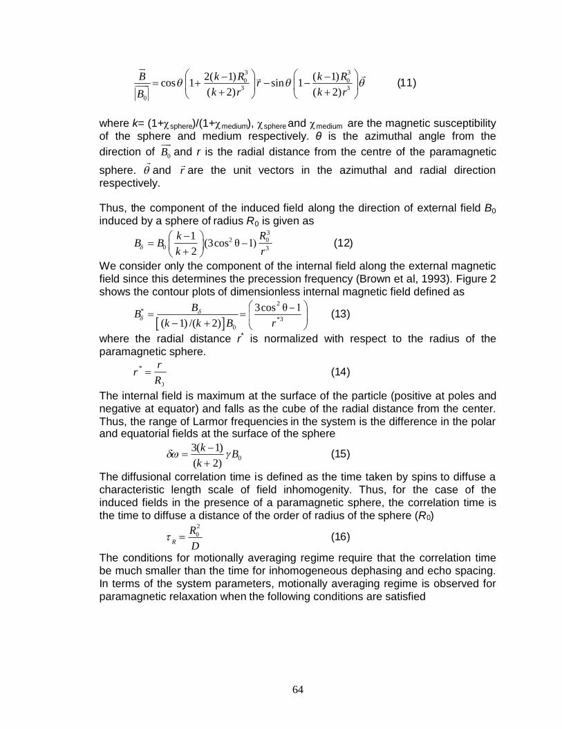
64
3 30 0
3 3
0
2( 1) ( 1)cos 1 sin 1( 2) ( 2)
k R k RB rk r k rB
(11)
where k= (1+sphere)/(1+medium), sphere and medium are the magnetic susceptibilityof the sphere and medium respectively. θ is the azimuthal angle from thedirection of 0B
and r is the radial distance from the centre of the paramagnetic
sphere.
and r
are the unit vectors in the azimuthal and radial directionrespectively.
Thus, the component of the induced field along the direction of external field B0induced by a sphere of radius R0 is given as
32 0
0 3
1(3cos θ 1)
2Rk
B Bk r
(12)
We consider only the component of the internal field along the external magneticfield since this determines the precession frequency (Brown et al, 1993). Figure 2shows the contour plots of dimensionless internal magnetic field defined as
2
**3
0
3cos θ 1( 1) /( 2)
BBk k B r
(13)
where the radial distance r* is normalized with respect to the radius of theparamagnetic sphere.
*
0
rr
R (14)
The internal field is maximum at the surface of the particle (positive at poles andnegative at equator) and falls as the cube of the radial distance from the center.Thus, the range of Larmor frequencies in the system is the difference in the polarand equatorial fields at the surface of the sphere
03( 1)( 2)
k Bk
(15)
The diffusional correlation time is defined as the time taken by spins to diffuse acharacteristic length scale of field inhomogenity. Thus, for the case of theinduced fields in the presence of a paramagnetic sphere, the correlation time isthe time to diffuse a distance of the order of radius of the sphere (R0)
20
R
RD
(16)
The conditions for motionally averaging regime require that the correlation timebe much smaller than the time for inhomogeneous dephasing and echo spacing.In terms of the system parameters, motionally averaging regime is observed forparamagnetic relaxation when the following conditions are satisfied

20
0
20
1 ( 2)3( 1)H
E
R kD k B
RD
(17)
The quantum-mechanical outer sphere theory (Gillis et al., 1987) suggests thatwhen conditions for motionally averaging are satisfied, the secular relaxation rateis given by
22
0 02,OS
1 4 16 ( 1)9 45 2R
kf f B R
T D k
(18)
where f is the volume fraction of the paramagnetic particles and is the rootmean square frequency at the surface of the sphere given as
0
4 ( 1)5 ( 2)
kB
k
(19)
Equation (18) is derived by solving quantum mechanical equations for the “fliprates” of the protons using time dependent perturbation theory (Gillis et al.,1987). Note the similar functional form of the secular relaxation rate predicted bythe outer sphere theory (equation 18) and equation 10b.
0.46
0.10.020.004
-0.46-0.1
-0.02
-0.004
Y*
Z*
Figure 2: Contour plots of z component of internal magnetic field (dimensionless)induced by a unit paramagnetic sphere in a vertical plane passing through the center
65
of the sphere. The external magnetic field is applied in the vertical z direction.

66
B. Free diffusion regimeFree diffusion regime is valid when half echo-spacing is the smallest of thecharacteristic time scales. The effect of restriction as well as large fieldinhomogenities is not felt by the spins in the time of echo formation. Thus, thespins dephase as if diffusing in an unrestricted medium. The conditions for freediffusion regime state
E H
E R
(20)
B.1 Free diffusion in constant gradientFor the case of diffusion in constant gradient in a pore, free diffusion regime oftransverse relaxation may arise for small echo spacings such that the spins donot experience the restriction effects. The conditions for free diffusion inside apore of length Ls can be obtained in terms of characteristic length scales definedin equations (2) and (3) by substituting equation (8) in equation (20) given as
s
d g
d
L L
L L
(21)
Thus, the free diffusion regime arises when the diffusion distance in E is muchsmall compared to dephasing length and pore length. In this regime, the secularrelaxation is given by the classical Bloch expression (Carr and Purcell, 1954) forunrestricted diffusion in a constant gradient
2 2 2
2,sec
13
Eg DT
(22)
The relaxation rate, thus, shows a quadratic dependence with echo spacing aslong as the conditions for free diffusion regime are satisfied.
B.2 Free diffusion in internal fields induced by paramagnetic particlesThe free diffusion regime has been described as the “weak magnetization regime( 1E )” in the medical resonance imaging (MRI) literature mentioned below.The regime arises physically when weakly magnetized paramagnetic particlesare used as contrast agents for medical imaging or in biological tissues with ironrich cells or deoxygenated red blood cells. Jenson and Chandra (2000) derivedthe expression for the secular relaxation in weak field inhomogenities byassuming a Gaussian field correlation function. Their solution was modified byBrooks et al (2001) to calculate the relaxation rate by weakly magnetizedparamagnetic particles which is given as
22 22
0 22,FD 0
2.25 ( )1 9 ( 1)5 ( 2)
EE
R
f k Df B
T k R
(23)
The above expression (called the Mean Gradient Diffusion Theory, MGDT)shows the similar quadratic dependence of secular relaxation rate on the echospacing as the expression for unrestricted diffusion in constant gradient (equation22). However, the relaxation rate shows an inverse squared dependence on theparamagnetic particle size which is opposite to that in the motionally averaging

67
regime (equation 18). This is because the mean squared internal field gradientgiven as
22
2 20
9 ( )fgR
(24)
decreases with the increase in particle size (Brooks et al., 2001). The meangradient in equation (24) is calculated by integrating the square of gradient of themagnetic field induced by a single paramagnetic particle (equation 11) overinfinite space.
C. Localization RegimeLocalization regime of secular relaxation arises when dephasing time is smallcompared to the diffusion correlation time and half echo spacing. The conditionsfor localization regime are
H R
H E
(25)
C.1 Localization regime in constant gradientUsing equations (8) for and R for restricted diffusion in constant gradient in apore of length Ls, equation (25) reduce to the following equations in special cases
g d
g s
L L
L L
(26)
The dephasing length is the smallest characteristic length in the localizationregime. Thus, the spins typically dephase a large amount during themeasurement time and do not contribute to the total magnetization. The signalcomes primarily from the spins near the boundaries which see smaller change inmagnetic field due to reflection (Sen et al., 1999). Localization regime is mostdifficult to treat theoretically because of the presence of large gradients. De Swietet al. (1993) have shown that at long times, the echo amplitude decays as
21( / )
0
( , ) d ga L LgE
s
LM g c eM L (27)
where a1=1.0188… and c=5.8841… for parallel plates. The exponent isindependent of the pore geometry but the prefactor is modified for othergeometries.
C.2 Localization regime in internal fields induced by paramagnetic particlesSecular relaxation in localization regime has also been discussed in the MRIliterature. The regime arises physically for relaxation in presence of stronglymagnetized contrast agents such as superparamagnetic particles for whichE>1. Gillis et al (2002) proposed a semi-empirical model for decay in internalfields induced by strongly magnetized spheres. In their model, the regionsurrounding the paramagnetic particle is divided in two regions: an inner regionwith very strong internal gradients and an outer region with only weak gradients.The boundary radius ( 'R ) between the inner and outer region is related to thesystem parameters as (Gillis et al., 2002)
68
1/ 3
0
' E
E
RR a bf
(28)
Since the gradients in outer region are weak, Gillis et al. (2002) suggested thatrelaxation can be described by theory for relaxation by weakly magnetizedparticles. Thus, the relaxation rate in the outer region (r> 'R ) is given by equation(23) with a modification to account for the excluded volume of the inner regionshown below
5/ 32 2
2,Loc
2.25 ( )1 E E
R E
fT a bf
(29)
where a and b are adjustable parameters. Gillis et al. (2002) calculated thevalues of the parameters a (=1.34) and b (=0.99) by fitting equation (29) tonumerical simulations of transverse relaxation in the presence of stronglymagnetized particles.
In the inner region (r< 'R ), the spins experience very strong gradient anddephase very fast. Due to very fast relaxation, they do not contribute much to themacroscopic relaxation rate and equation (29) can provide a good measure ofrelaxation rate for strongly magnetized particles.
D. Parametric representation of relaxation regimesThe asymptotic regimes of secular relaxation are schematically shown in figure 3as a function of two dimensionless parameters: R and E. The boundariesbetween the asymptotic regimes are drawn at the equality between thecharacteristic times. Thus, the regimes are typically valid in the regions awayfrom the boundaries.

69
III. Random Walk simulations
The decay of transverse relaxation due to diffusion in inhomogeneous fields isstudied with the help of random walk simulations. The simulations provide aconvenient method to quantitatively study the characteristics of asymptoticregimes. We begin by numerically simulating the secular relaxation ininhomogeneous field induced in the annular region of a paramagnetic particle.Surface relaxation at the inner radius (R0) and outer radius (Re) of the annulus isneglected. Measurement of spin-echoes by CPMG pulse sequence techniquewith ideal pulses is simulated.
The relaxation of transverse magnetization (M) in an inhomogeneous field Bz
after the application of first /2 pulse is given by the Bloch- Torrey equations2
2,z
B
M Mi B M D M
t T
(30)
10-2 10 -1 100 101 102 10310-2
10-1
100
101
102
103
R=R/H
E=
R/
H
Motionallyaveraging
Localization
Free Diffusion
H<<RH<<E
E<<RE<<H
R<<HR<<E
Figure 3: Schematic diagram of asymptotic relaxation regimes in the (R, E)parameter space.

70
where D is the diffusivity of the fluid and T2,B is the bulk relaxation time. Nosurface relaxation at the inner and outer boundaries implies
0n M
at r = R0. (31)
0n M
at r= Re. (32)Here r is the radial distance from the center and n
is the outward pointing
normal.
By substituting yx iMMM and
BTt
ti
emM 20
(where 00 B ),equation (30) can be expressed as
mDmBitm
z2
(33)
where Bz = Bz-B0. m represents the transverse magnetization with theprecession at Larmor frequency (0) and bulk relaxation factored out (Zhang andHirasaki, 2003)
Let us now introduce the following dimensionless variables*
e
rrR
, *
0
ttt
, *
0
mmM
where t0 is a characteristic time and M0 is the initial magnetization. Substitutingthe dimensionless variables and equation (12) for field induced by aparamagnetic sphere in (33), we get
3* 2* *2 *0 0
0* *3
( 1)(3cos 1)( 2) D
e
B k Rmi t m N m
t r k R
(34)
where dimensionless group ND is defined as0
2De
DtNR
(35)
Now, the characteristic time t0 is chosen such that the coefficient of the secondterm in equation (34) is unity. Thus,
00
( 2) 1( 1)
kt
B k f
(36)
where f is the volume fraction of the paramagnetic particle given as3
0
e
Rf
R
(37)
The term in parenthesis in the expression for t0 (equation 36) is the reciprocal ofthe equatorial frequency shift (magnitude) at the surface of the paramagneticsphere. This cane be verified by using = /2 and r = R0 in equation (12).
0( 1)( 2)eqt
k Bk
(38)

71
Thus, t0 can be expressed as reciprocal of the product of equatorial frequencyshift and the volume fraction.
0
1
eqt
tf
(39)
Equation (39) is used to normalize secular relaxation rates for the experimentalsystems as described in Section IV. The dimensionless parameter, ND, can alsobe expressed in terms of system parameters by substituting equation (36) inequation (35)
02 3
0 0
( 2)( 1)
eD
e
Dt k DRN
R k B R
(40)
Thus, the governing Bloch equation in dimensionless form becomes* 2
* *2 ** *3
(3cos 1)D
mi m N m
t r
(41)
The dimensionless boundary conditions are*
* 0mr
at r*=1 (42)
*
* 0mr
at * 0
e
RrR
(43)
In addition, the application of pulse at dimensionless half-echo time E*
reverses the y component of the magnetization. Thus,
* ** *| |t tm m at t*=E
*, 3E*, 5E
*….E* (44)
E* is the dimensionless echo spacing given as
E* = E/t0. (45)
A. AlgorithmA continuous random walk algorithm is applied to model T2 relaxation of spins(equations 41-45) diffusing in an inhomogeneous internal field Bz(r,) (Weisskoffet al, 1994). The random-walkers are initially distributed uniformly in an annularregion of spherical paramagnetic particle. The outer radius was taken to be 20times the radius of the concentric paramagnetic particle (Re=20R0). Since themagnetic field falls as the cube of the particle radius, the field becomes negligiblein the region greater than 10 times the inner radius. Thus, an outer radius of20R0 is sufficient to avoid any boundary effects (Weisskoff et al, 2000).
The walkers start with a zero initial phase. In dimensionless time step dt*, the nth
walker at a position (r*,*) accumulates a phase of n=*(r*,*)dt*. Thedimensionless Larmor frequency * is given as

72
2* * *
*30
( , ) (3cos 1)( , )1/rrt r
(46)
After every time step dt*, the stochastic diffusion of the proton is simulated bychoosing a random displacement with zero mean and standard deviation
*2 DN dt in the x, y and z directions in Cartesian coordinates. The clock inincremented by dt* after every time step.
At the time of the application of pulses t*=E*,3E
*,5E*…., the phases of all
random walkers is inverted. Perfect reflection at the inner and outer boundaries issimulated by returning the walker to the same position if the next displacementtakes it outside the boundaries. The echo intensity at times t*=2E
*,4E*,6E
* … isevaluated by averaging the phases of all walkers
* *
1
1( ) exp( ( ))
N
nn
M t i tN
(47)
where N is the number of walkers and n(t*) is the phase of the nth walker at timet*. The dimensionless relaxation rate is calculated from the slope of exponentialfit to the simulated echo intensities. However, magnetization decay is multi-exponential for simulations such that R>100. For such cases, relaxation rateis calculated from the slowest rate of the multi-exponential decay.
There are two simulation parameters which should be appropriately chosen toensure the accuracy of the solution
1. Number of walkers (Nw) – Number of walkers determines the statisticalnoise in the simulations. Simulations with different number of walkersshowed that N=10,000 gives a good accuracy (<0.1% average absolutedeviation from the analytical solutions) and a reasonable amount ofcomputational time.
2. Time step (dt*) – The value of the time step should be so chosen such thatthe dimensionless diffusion length in time step dt* is less than anydimensionless characteristic length of the system. Since the radius of theparamagnetic particle sphere is the smallest characteristic length, dt* waschosen such that
* 02 De
RN dtR
(48)
B. ValidationThe random walk simulations are validated for unrestricted and restricteddiffusion in constant gradient by comparing with the known analytical expressionsfor transverse relaxation in the two cases.
B.1 Unrestricted Diffusion in constant gradientFor unrestricted diffusion in a constant gradient, echo attenuation due to diffusionfollows an exponential decay with a time constant given by the Bloch formula

73
(equation 22). Figure 4 shows the comparison between the analytical and thesimulated echo decay for the case of g=100G/cm and E = 2ms. The twosolutions match within 0.1% absolute average deviation indicating the validity ofthe algorithm. The algorithm was validated for more cases and for each case thesolutions matched within good agreement.
B.2 Restricted Diffusion in constant gradientFor the case of restricted diffusion, random walk simulations are validated bycomparing with the analytical expression for transverse relaxation in constantgradient inside a sphere. In the motionally averaging regime, relaxation due todiffusion in a constant gradient g in a sphere of radius Rs is given as (Neumann,1974)
4 2 2
2
81175
sR gT D
(49)
The simulations are done in terms of dimensionless variables by normalizing thespatial variables with the radius of the sphere (Rs). Thus, the normalizedcharacteristic lengths (equations 2 and 3) are given as
g*3
1=g
s s
L DL
R R g (50)
0 0.05 0.1 0.15 0.2 0.25 0.3 0.35 0.4 0.45 0.510-2
10-1
100
Time (sec)
M/M
o
Analytical Echo DecaySimulated Echo Decay
Figure 4: Comparison of analytical and simulated echo decay for unrestricteddiffusion in constant gradient. The parameters used in the simulations areg=100G/cm, E = 2ms, Nw=10,000 and dt=0.1μs.
74
* dE
1=ds s
LL DR R
(51)
The temporal variable is normalized with a characteristic time (tc) defined as1
cs
tgR
(52)
tc defines the characteristic time for relaxation in constant gradient in contrast tot0 (equation 36) which was defined for relaxation in the presence of paramagneticparticle. The expression for tc is derived by following the same procedure as wasused to derive t0 expect that the inhomogeneous field (Bz) is for a constantgradient given as
zB gz (53)
Secular relaxation due to diffusion in constant gradient with Lg* = 1.2 and 1.5 is
numerically simulated. For each case, two values of Ld* =2 and 3 (i.e two echo
spacings) are chosen. The values of Lg* and Ld
* were chosen greater than one sothat the systems are in motionally averaging regime and relaxation rate is givenby equation (49) normalized by characteristic rate 1/tc. Figures 5 and 6 show thecomparison between simulated and analytical echo decay for two cases with Lg
*
= 1.2 and 1.5 respectively. The two cases of Ld* =2 and 3 are shown in the upper
and lower panel of the figures. For all cases, the simulated and analytical echoamplitudes match very well (<1% absolute average deviation) indicating thevalidity of the numerical technique.

75
0 20 40 60 80 100 120 14010
-2
10-1
100
Time (dimensionless)
M/M
0
0 20 40 60 80 100 12010-2
10-1
100
Time (dimensionless)
M/M
0
Analytical Echo DecaySimulated Echo Decay
Figure 5: Comparison of simulated and analytical echo decays for restricted diffusion in asphere with constant gradient. The parameters used in the simulations are Lg
* = 1.2 and Ld*
= 2 (upper panel) and Ld* = 3 (lower panel). Lesser number of points in the lower figure is
due to smaller sampling rate with larger Ld*. The analytical rate is given by equation (49)
normalized by 1/ tc.

76
C. ResultsWe now present the results for random walk simulations of secular relaxation inthe presence of paramagnetic particles. Secular relaxation of protons in thepresence of paramagnetic particle of susceptibility 0.2 (SI units) and radiusranging from 20nm to 2μm is simulated. The value of susceptibility isrepresentative of magnetite. The external magnetic field B0 corresponds to aproton Larmor frequency of 2MHz. For each particle size, simulations withdifferent values of half echo spacing are performed to study the echo spacingdependence of secular relaxation in different regimes. Thus, the simulations spanthe entire (R, E) parameter space of figure 3.
Figure 7 shows the plot of simulated dimensionless relaxation rates as a functionof R for different cases of E where is the equatorial frequency shiftgiven by equation (38). The solid black line is the plot of theoretical relaxationrate (equation 18) in the motionally averaging regime normalized by thecharacteristic rate 1/t0 (Brooks et al, 2001)
0 50 100 150 200 25010-2
10-1
100
Time (dimensionless)
M/M
0
0 50 100 150 200 25010
-2
10-1
100
Time (dimensionless)
M/M
0
Analytical Echo DecaySimulated Echo Decay
Figure 6: Comparison of simulated and analytical echo decays for restricteddiffusion in a sphere with constant gradient. The parameters used in thesimulations are Lg
* = 1.5 and Ld* = 2 (upper panel) and Ld
* = 3 (lower panel). Lessernumber of points in the lower figure is due to smaller sampling rate with larger Ld
*.The analytical rate is given by equation (49) normalized by 1/ tc.

77
0
2,sec 2,OS
1 16( , )
45 R R E HD
tT T
(54)
The superscript “D” refers to dimensionless relaxation rate. The dotted line is thenormalized relaxation rate (equation 23) given by mean gradient diffusion theoryvalid in the free diffusion regime (Brooks et al., 2001)
2 2 20
2,sec 2,FD
9( ) 9( )1( , )
5 5E E
E R HDR R
tT T
(55)
The dash-dotted lines are the plots of normalized relaxation rates (equation 29)given by modified mean field gradient theory (Brooks et al., 2002) valid in thelocalization regime given as
5/32 2
0
2,sec 2,Loc
4 59( )1 ( , )5 4 5
EEH E RD
R E
tT T a bf
(56)
The dashed line marks the boundaries R=1 and E =1 that delineate theasymptotic regimes.

Aasvir
FstpTp
10-2 10-1 100 101 102 10310-5
10-4
10-3
10-2
10-1
100
101
R
1/T 2,
sec
D
E=1000E=100E=10E=1E=0.3
E=0.1
MotionallyAveraging
Localization
Free Diffusion
1000
100
10
1
0.3
0.1
E
Fig 7: Plot of simulated secular relaxation rate (dimensionless) with R as a functionof E. The parameters used in the simulations are f= -41.25 10 ,k=1.2, B0= 496 Gauss.The solid, dashed and dotted line are the theoretically estimated secular relaxation ratesaccording to the outer sphere theory (equation 54), modified mean gradient diffusiontheory (equation 55) and mean gradient diffusion theory (equation 56) plotted in the
78
s was shown in Figure 3, the secular relaxation is characterized by threesymptotic regimes based on the values of R and E. For R <1 andufficiently large values of E >>1 in figure 7, motionally averaging regime isisible. The secular relaxation rates are independent of the echo spacing andncrease with particle size. The theoretically predicted outer-sphere relaxationates (equation 54) match well with the simulations as long as R <<1.
or R >1 and large values of E>>1, localization regime exists. Theecular relaxation rate shows strong dependence on echo spacing. In addition,he dependence of the relaxation rate on the correlation time (and thus thearticle size) is inversed compared to that in the motionally averaging regime.he relaxation rates now decrease with the particle size. This is because as thearticle size increases, the average internal field gradient decreases according to
respective regimes of validity.

79
equation (24). For R >>1, the simulated relaxation rates match well with thepredictions of modified MGDT (equation 56).
The free diffusion regime is valid for the smaller echo spacings E <1 as longas E<R. Since the decay is only weak in the free diffusion regime (Sen etal., 1999), the simulated relaxation rates are significantly smaller than the ones inlocalization or motionally averaging regime. For R >1, the relaxation ratesshow inverse dependence on the particle size due to decrease in magnetic fieldgradient with particle size. The simulated rates match well with the predictions ofthe mean gradient diffusion theory (equation 55).
Now, let us study the characteristics of the secular relaxation rate in the (R,E) parameter space. Figure 8 shows the contour plots of the dimensionlesssecular relaxation rate in the (R, E) domain. The boundaries between theasymptotic regimes are shown by dashed lines. We notice that in the motionallyaveraging regime (R<<1, E>>1), the contour plots are almost parallel tothe E axis implying that the relaxation rates are independent of the echospacing. Also, the rates increase with R showing that the secular relaxationincreases with particle size. In the localization and free diffusion regimes, thedependence of relaxation on R is reversed and the rates decrease withparticle size. In addition, the rates are echo spacing dependent. The contours aremore closely spaced and have lesser slope in the free diffusion regime than inthe localization regime. Thus, the dependence of the relaxation rate on the echospacing is higher in free diffusion than in the localization regime.

80
The echo spacing dependence of the simulated rates in the different regimesneeds to be quantitatively studied. Figure 9 shows the plot of simulatedrelaxation rate with dimensionless echo spacing E for cases in which R <1.The dashed curve shows the boundary E = R delineating the free diffusionand motionally averaging regime. In the motionally averaging regime, therelaxation rates increase with particle size in accordance to the predictions ofouter sphere theory. In addition, the relaxation rates are dependent on echospacing in the free diffusion regime while they are independent of the echospacing in the motionally averaging regime.
Figure 10 shows the plot of simulated relaxation rates with E for cases inwhich R >1. The dashed line shows the boundary E =1 between the freediffusion and localization regime. Note the large decrease in the slope ofrelaxation rates as the systems transition from the free diffusion to thelocalization regime. In addition, the dependence of the relaxation rate on theecho spacing is almost linear in the localization regime.
10-1 10 0 101 102
100
101
102
R
E
0.60.6
0.36
0.13
0.04
0.04
0.07
0.02
0.2
0.07
0.04
0.01
0.02
MotionallyAveraging
Localization
Free Diffusion
0.36
Figure 8: Contour plots of dimensionless secular relaxation rate in the (R, E)parameter space.

81
10-1
100
101
102
103
10-3
10-2
10-1
100
E
1/T
2,se
cD
R=0.75
R
=0.33
R=0.08
R=0.02
Motional Averaging RegimeFree DiffusionRegime
Figure 9: Plot of secular relaxation rates (dimensionless) with dimensionless echospacing E for R <1. The dashed line is the boundary E =R delineating thefree diffusion and motionally averaging regime. The relaxation rates are almostindependent of echo spacing in the motionally averaging regime.

82
Note that even though the simulations were done for inhomogeneous fieldinduced by a single paramagnetic particle, the above arguments would bequalitatively similar in other field distributions as well.
IV. ExperimentalIn the previous sections, we described the classification of different regimes oftransverse relaxation based on three characteristic time (or correspondinglength) scales. In the next section, we describe a series of proton relaxationmeasurement with paramagnetic particles spanning a size range from angstromsto microns. These measurements explain the characteristics of the relaxationregimes as a function of the length scale of field inhomogenity. The section isorganized in two subsections. In the first subsection, we describe the protonrelaxation measurements with aqueous dispersions of paramagnetic particles ofvarious sizes. The experiments help to quantitatively estimate the characteristictime scales for secular relaxation in the presence of paramagnetic particles. Inthe second subsection, experiments with sand coated with paramagneticparticles of various sizes are described.
10 -1 100 101 102 10310-4
10-3
10-2
10-1
100
101
E
1/T 2,
sec
D
R=3
R=12R=48R=196
Free DiffusionRegime
LocalizationRegime
Figure 10: Plot of secular relaxation rates (dimensionless) with dimensionless echospacing E for R >>1. A dashed line is the boundary E =1 delineating the freediffusion and localization regime. Note the linear dependence of the relaxation rate in thelocalization regime.
A. Paramagnetic particles in solution
A.1 Ferric ionThe smallest paramagnetic particle studied was ferric ion (hydrated ionic radius2.62A, Bertini et al., 1993). Solutions of ferric chloride were made at varioussolute concentrations in 0.1N Hydrochloric acid. Acidic pH of the solutionsprevents the formation of hydroxides. Proton longitudinal and transverserelaxation of the solutions was measured at 30oC. The T2 relaxation wasmeasured with different echo spacings to study the echo spacing dependence.Figure 11 shows the T1 and T2 relaxation rates of the aqueous solution of ferricions as a function of the solution concentration.
Tcdtr
ATaA
10-5 10-4 10-3 10-210-3
10-2
10-1
100
Conc (g/ml)
1/T 1,1
/T2
(ms)
-1
1/T2
1/T1
Figure 11: Longitudinal and Transverse relaxation rates of ferric chloride solutions as
83
he relaxation rates of the ferric solutions increase linearly with theoncentration. Furthermore, the T1/T2 ratio is unity and no echo spacingependence of transverse relaxation is observed. T1/T2 ratio of unity implies that
he secular relaxation does not contribute significantly to the transverseelaxation.
.2 Polymer Coated Magnetite Nanoparticleso explore a larger length of field inhomogenity, NMR proton relaxation ofqueous dispersions of magnetite nanoparticles of various sizes was studied.queous dispersions of the nanoparticles were obtained from Dr. V. Colvin’s Lab.
a function of the concentration of the solution.

84
The nanoparticles were synthesized by the pyrolysis of iron carboxylate salts inan organic solvent and subsequently dispersing the nanoparticles in water (Yu etal., 2004). Particles are then coated with a layer of a polymer which preventsagglomeration of the particles in external magnetic field due to interparticle dipoleattraction. The size of the particles can be controlled by changing the time ofreaction. Figure 12 shows the TEM images of 4nm, 9nm and 16nm magnetiteparticles (Agarwal, S., 2007) used in our study.
Proton relaxation rates of the aqueous dispersions were measured as a functionof the concentration of the dispersion. Figure 13 shows the plots of longitudinal,transverse and secular relaxation rates with the concentration of the dispersionfor the three particle sizes. The solid lines are the linear best fits of theexperimental points. Once again, we notice that the relaxation rates increaselinearly with the concentration of the paramagnetic particles. No echo spacingdependence of the T2 relaxation is observed. In contrast to the ferric ions,however, the T1/T2 ratio is greater than one and increase monotonically with theparticle size (Figure 14).

Figure 12: TEM(b) 9nm magneti
(a)
(b)
(c)images of magnetite nanoparticles. (a) 4nm magnetite
85
te (c) 16nm magnetite (Agarwal,S., 2007).
86
0 0.5 1 1.5 2 2.5 3
x 10-4
0
0.005
0.01
0.015
0.02
0.025
0.031/
T1,
2(ms)
-1
0 1 2 3 4 5 6 7
x 10-5
0
0.005
0.01
0.015
0.02
1/T
1,2(m
s)-1
0 0.2 0.4 0.6 0.8 1 1.2
x 10-4
0
0.02
0.04
0.06
0.08
Concentration (g/ml)
1/T 1,
2(ms)
-11/T
21/T
11/T
2,sec
y=135x
y=96x
y=39x
y=257x
y=162x
y=95x
y=699x
y=369x
y=320x
Dp=4nm
Dp=9nm
Dp=16nm
Figure 13: Plot of transverse, longitudinal and secular relaxation rates of aqueousdispersions of magnetite nanoparticles of three different sizes with the concentration ofthe dispersion. The diameter of the nanoparticles (Dp) and slopes of the linear best fitsare also mentioned.

APuncpitrpl
Ldt(wpito
10-1 100 101 102 1031
1.1
1.2
1.3
1.4
1.5
1.6
1.7
1.8
1.9
2
Particle Diameter (nm)
T 1/T
2
Polymer Coated nanoparticlesSynthesized nanoparticles
Figure 14: T1/T2 ratio of the aqueous dispersions of paramagnetic particles as afunction of the particle size. The T1/T2 ratio increases with the particle size in the
87
.3. Magnetite nanoparticles coated with citrate ionositively charged magnetite nanoparticles of different sizes were synthesizedsing Massart’s Method (1981). The aim of synthesizing positive chargeanoparticles is to adsorb them on the negatively charged silica surface byolumbic attraction. Thus, relaxation characteristics of model sandstones witharamagnetic particles adsorbed at different concentrations can be studied. This
s not possible for the polymer coated nanoparticles since the coating preventshe particles from adsorbing on the sand surface. Here we will describe theelaxation characteristics of aqueous dispersions of the positively chargedarticles. NMR experiments with particles coated on sand will be described in a
ater section.
et us first describe the experimental procedure used to obtain stable magnetiteispersions. Nanoparticles are synthesized by co-precipitation of magnetite from
he aqueous solution of ferrous and ferric chloride using ammonium hydroxideMassart,R.,1981). The precipitated magnetite is washed with 2M perchloric acidhich makes the nanoparticles positively charged due to surface adsorption ofrotons (Massart,R.,1981). The positively charged particles can then be peptized
n excess of water. The size of the particles can be controlled by changing theemperature of the reaction. At higher temperature, larger sized particles arebtained due to Oswald ripening. Figure 15 shows the particle size distribution
motionally averaging regime.

88
obtained by dynamic light scattering for two sets of nanoparticles. The averagediameters of the particles for the two sets are 25nm and 110nm respectively.The 25nm particles are synthesized at 10oC while 110nm particles aresynthesized at room temperature.
In the absence of external magnetic field, the positive charge on the particleshelps to prevent the particles from agglomeration due to interparticle dipoleattractions. However, the weak columbic repulsion is not sufficient to preventagglomeration in the presence of external fields. Thus, the nanoparticles werestabilized by adding 1M sodium citrate in the volume ratio of 1%. Strong stericand columbic repulsion between citrate coated particles prevents them fromagglomeration.
Proton relaxation rates of aqueous dispersions of the citrate coated particleswere measured as a function of the concentration. Figure 16 shows the plots oflongitudinal, transverse and secular relaxation rates with the concentration of thedispersion for the two particle sizes. The linear best fits of the experimentalpoints and the corresponding slopes are also shown. The results arecomparable to those for the aqueous dispersions of polymer coated magnetite.Relaxation rates are linearly dependent on the concentration of the dispersionand no echo spacing dependence of T2 relaxation rates is observed. The T1/T2ratio is also greater than one and increases with particle size (Figure 14).
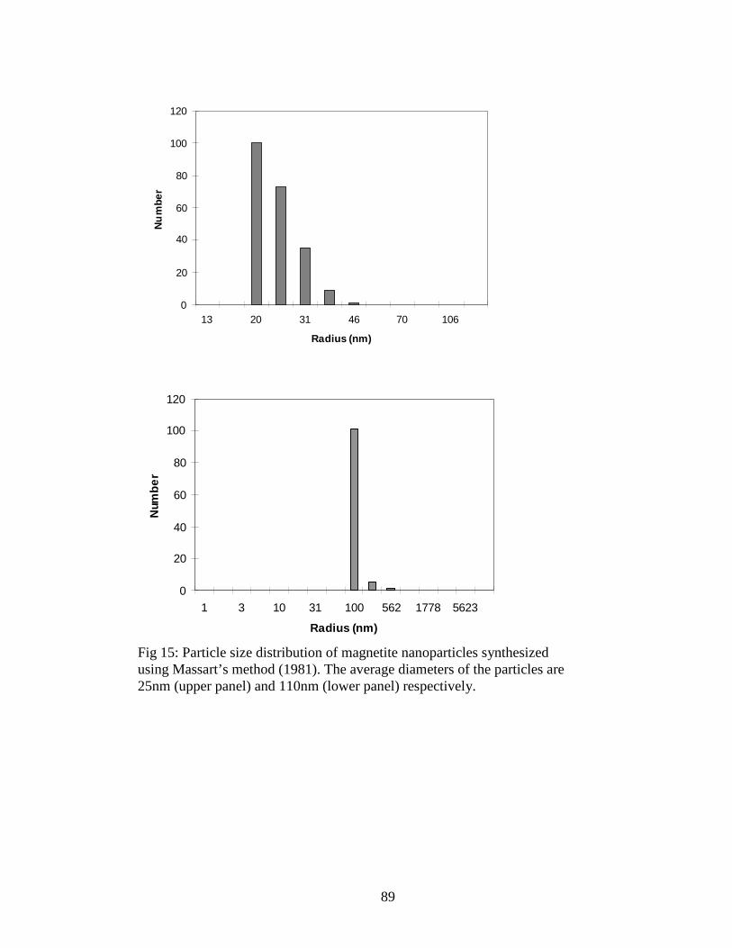
89
0
20
40
60
80
100
120
13 20 31 46 70 106
Radius (nm)
Nu
mbe
r
0
20
40
60
80
100
120
1 3 10 31 100 562 1778 5623
Radius (nm)
Num
be
r
Fig 15: Particle size distribution of magnetite nanoparticles synthesizedusing Massart’s method (1981). The average diameters of the particles are25nm (upper panel) and 110nm (lower panel) respectively.

AArmacpapp
Lpfecw
0 0.2 0.4 0.6 0.8 1 1.2
x 10-3
0
0.05
0.1
0.15
0.2
1/T
1,2(m
s)-1
0 1 2 3 4 5 6
x 10-4
0
0.05
0.1
0.15
0.2
Concentration (g/ml)
1/T
1,2(m
s)-1
1/T2
1/T1
1/T2,sec
Dp=25nm
Dp=110nm
y= 190x
y= 118x
y=72x
y=239x
y= 140x
y=99x
Figure 16: Plot of transverse, longitudinal and secular relaxation rates of aqueousdispersions of magnetite nanoparticles of two different sizes with the concentrationof the dispersion. The radii of the nanoparticles (Dp) and slopes of the linear best fits
90
.4 Discussions was described earlier, secular relaxation can be characterized by three
elaxation regimes depending on the smallest characteristic time scale. In theotionally averaging regime, secular relaxation is independent of echo spacing
nd increases with the particle size and concentration. Similar relaxationharacteristics are also observed for aqueous dispersions of submicronaramagnetic particles. No echo spacing of transverse relaxation is observednd the T1/T2 ratio increases with the particle size. We, thus, hypothesize that theroton relaxation of the aqueous dispersions of (submicron) paramagneticarticles is in the motionally averaging regime.
et us now quantitatively evaluate the characteristic time scales (E,R,H) torove the validity of the hypothesis. The value of half echo spacing (E) is knownrom the experimental measurements. In our measurements, the smallest halfcho spacing used was 0.2ms. The diffusional correlation time (R) can bealculated from the radius of the paramagnetic particle (R0) and diffusivity ofater at 30oC (~ 52.5 10 cm2/sec) by using the following equation
are also mentioned.

91
20
R
RD
(57)
Under the assumption of motionally averaging regime, the expression for thesecular relaxation rate can be used to estimate for the magnetitenanoparticles as shown below.
2
2,sec
1 1645 Rf
T (58)
2
2,sec
16145
R CT d
(59)
where C is the concentration of the dispersion and d is magnetite density. Thus,from the slopes of the plots between secular relaxation and the concentrationgiven in figures 13 and 16, can be evaluated for the various particle sizes. H
is obtained as the reciprocal of . Table 1 lists the characteristic time scales forthe different particles. We notice that R< H, E for all cases (except for 110nmparticle for which R~H) and thus our earlier hypothesis of motionally averagingregime is justified.
Thecondition R<< E implies that the magnetic field inhomogenities are motionallyaveraged in time much smaller than E. Thus, no dependence of T2 relaxation onecho spacing is observed for the aqueous dispersions of ferric ions andmagnetite nanoparticles. Additionally, the secular relaxation rate is proportionalto the square of the radius of the paramagnetic particle in the motionallyaveraging regime. Due to very small size of the ferric ion, the secular relaxationcontributes negligibly to the transverse relaxation and the T1/T2 ratio is unity.Secular relaxation, however, increases for the larger sized particles andcontributes significantly to the T2 relaxation. Thus, the T1/T2 ratio increases withparticle size (provided the susceptibility remains same) as observed in Figure 14.The larger T1/T2 ratio for the polymer coated nanoparticles is probably due to ahigher magnetic moment.
Table 1: Characteristic Time scales for the ferric and magnetite nanoparticles.
TimeScale(sec)
Fe3+ 16nm 9nm 4nm 25nm 110nm
R113 10 83 10 98 10 92 10 86 10 610
E,minimum42 10 42 10 42 10 42 10 42 10 42 10
H32 10 88 10 88 10 85 10 72 10 610

92
B. Paramagnetic particles on silica surface
Next, we will describe the proton relaxation for water-saturated fine sand coatedwith paramagnetic particles. Coated sand serves as a model to quantitativelyunderstand the paramagnetic relaxation mechanisms in sandstones. Sand iscoated with particles of various sizes and concentrations to explain the transitionof the relaxation regimes as the length scale of field inhomogenity increases. Thetheory is then applied to describe relaxation in North-Burbank sandstone whichhas strong internal gradients induced due to pore lining chlorite flakes (Zhang etal., 2003).
B.1 Sand coated with Ferric ionsLet us first describe the experimental protocol used to coat fine sand (SigmaAldrich) with paramagnetic ferric ions. Fine sand (grain radius 50μm) wasrepeatedly washed with fresh batches of hydrochloric acid till the relaxation timeof the washing acid stopped changing. Washing with acid helps to remove theparamagnetic particles already present on the sand surface. The sand was thenexhaustively washed with deionized water and dried. A known quantity (15grams) of the dried sand was kept in contact with acidic (pH 1) solutions of ferricchloride of known concentrations for 24 hours in a plastic bottle. The solid toliquid ratio (gm sand/ml) of the slurries was kept at 1:10. Low pH (<7) of the ferricsolutions helps to prevent the formation of hydroxides and precipitation on thesand surface. To ensure uniform coating, the slurries were constantly rotatedwhich prevents the sand from settling at the bottom. After 24 hours, thesupernatant was removed and the coated sand was exhaustively washed withdeionized water. This last step removes any remaining ferric ions in the poreliquid. Thus, the relaxation of the pore liquid can only be attributed to surfacerelaxation and diffusion in internal field gradients.
The surface concentration of the ferric ions can be estimated by measuring thequantity of the ferric ions deposited on a known surface area of sand asdescribed. The BET surface area of sand (0.2 m2/g) was determined using N2adsorption at 77K. To estimate the deposited quantity, the relaxation time of thesupernatant was measured. Using the calibration between the concentration offerric ion solution and the relaxation rate (Figure 11), the concentration of thesupernatant can be determined. The difference in the concentrations of thesupernatant and initial coating solutions multiplied by the volume of the solutiongives the quantity deposited on the sand surface.
Figure 17 shows the T1 and T2 distributions of the sand coated with ferric ions atvarious surface coverages expressed as surface area/ion. Table 2 lists themodes of the relaxation time distributions for the various cases. No echo spacingdependence of T2 relaxation is observed and the T1/ T2 ratio of coated sand isclose to that of washed sand at all concentrations.

Table 2: Longitudinal and transverse relaxation times of water-saturated finesand coated with ferric ions at different surface coverages (area/ferric ion).
Concentration(Area/particle)
Washedsand 0.3nm2/Fe3+ 0.09nm2/Fe3+ 0.03nm2/Fe3+
T1 (ms) 1587 471 372 294
93
T2 (ms) 1260 378 294 233

94
0
0.1
0.2
0.3
0.4
1.00E-01 1.00E+00 1.00E+01 1.00E+02 1.00E+03 1.00E+04
T1,T2(ms)
f
T2T1
0
0.5
1
1.5
2
1.E-01 1.E+00 1.E+01 1.E+02 1.E+03 1.E+04
T1,T2(ms)
f
0
0 .05
0.1
0 .15
1.E-01 1.E+00 1 .E+01 1.E+02 1 .E+03 1 .E+04
T1 ,T2 (m s)
f
0
0.2
0.4
0.6
0.8
1.E-01 1.E+00 1.E+01 1.E+02 1.E+03 1.E+04
T1,T2(ms)
f
T2,tau=0.2ms
T2,tau=1ms
T1
Figure 17: T1 and T2 distributions of fine sand coated with ferric ions at differentsurface concentrations.
0.3nm2/part.
0.09nm2/part.
0.03nm2/part.
Washed Sand

95
B.2 Fine Sand coated with magnetite nanoparticlesKnown quantity of fine sand was coated with 25nm and 110nm magnetiteparticles by following the same procedure as that for the ferric ions. Theconcentration of the coating dispersion was varied to obtain different surfaceconcentrations of magnetite. Note that the coating is done with positively chargedmagnetite not coated with citrate ion. Figure 18 and 19 show the T1 and T2distributions of water-saturated fine sand coated with 25nm and 110nmmagnetite as a function of surface concentration. Table 3 and 4 lists the modesof the relaxation time distributions for the different cases.
We notice that at low surface concentrations of either 25nm or 110nm particlesno echo spacing dependence of transverse relaxation is observed. At the highestconcentration, however, an echo spacing dependence of T2 relaxation isobserved for both cases. As will be described in the interpretation section, thisecho spacing dependence is observed because at high concentrations theparticles form a shell around each silica grain such that the length scale of theregion of induced magnetic gradients is large compared to the diffusion lengthduring the time of the echo spacing.
Table 3: Longitudinal and transverse relaxation times of water-saturated fine sandcoated with 25nm magnetite at different surface coverages.
Concentration(Area/particle)
33 10 nm2/particle 410 nm2/particle. 49 10 nm2/particle.
T1 23.6 42 343
T2 (E = 0.2ms) 18.7 29 215
T2 (E = 0.5ms) 16.6 29 215
T2 (E = 1ms) 11.7 29 215
T2 (E = 2ms) 8.30 29 215

.B.3
Thesizemagsho2.4μreladepratio
Table 4: Longitudinal and transverse relaxation times of water-saturated fine sandcoated with 110nm magnetite at different surface coverages.
Concentration(Area/particle) 0.3 μm2/particle 8 μm2/particle. 30 μm2/particle.
T1 24 95 613
T2 (E = 0.2ms) 21 63 385
T2 (E = 0.5ms) 20 63 385
T2 (E = 1ms) 16.6 63 385
96
Fine Sand with dispersed 2.4μm magnetite
length scale of field inhomogenity can also be increased by increasing theof the paramagnetic particle. Fine sand (15gms) was dispersed with 2.4μmnetite (Fischer Scientific) dispersions of known concentrations. Figure 20
ws the T1 and T2 distribution of water saturated fine sand with dispersedm magnetite at two concentrations. The corresponding modes of thexation time distributions for the two cases are listed in Table 5. Note aendence of transverse relaxation on echo spacing is observed and the T1/ T2
is greater than 2.
Table 5: Longitudinal and transverse relaxation times of water-saturated fine sand with dispersed 2.4m magnetite.
.Relaxation time(ms) 2.7 cm2/particle. 0.9 cm2/particle.
T1 486.3 272T2 (E = 0.2ms) 215.4 75.6
T2 (E = 0.5ms) 170.7 47.5
T2 (E = 1ms) 135.3 37.6
T2 (E = 2ms) 105.2 21.0
T2 (E = 2ms) 14.8 63 385
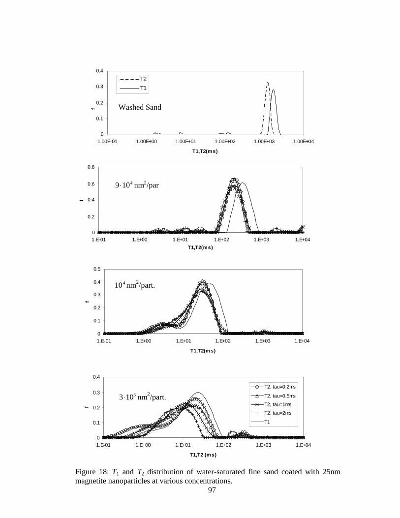
0
0.1
0.2
0.3
0.4
1.00E-01 1.00E+00 1.00E+01 1.00E+02 1.00E+03 1.00E+04
T1,T2(ms)
f
T2
T1
0
0.2
0.4
0.6
0.8
1.E-01
f
0
0.1
0.2
0.3
0.4
0.5
1.E-01
f
0
0.1
0.2
0.3
0.4
1.E-01
f
Figure 18:magnetite n
Washed Sand
49 10 nm2/par
97
1.E+00 1.E+01 1.E+02 1.E+03 1.E+04
T1,T2(ms)
1.E+00 1.E+01 1.E+02 1.E+03 1.E+04
T1,T2(ms)
1.E+00 1.E+01 1.E+02 1.E+03 1.E+04
T1,T2 (ms)
T2, tau=0.2ms
T2, tau=0.5ms
T2, tau=1ms
T2, tau=2ms
T1
T1 and T2 distribution of water-saturated fine sand coated with 25nmanoparticles at various concentrations.
t.
410 nm2/part.
33 10 nm2/part.

98
0
0.1
0.2
0.3
0.4
1.00E-01 1.00E+00 1.00E+01 1.00E+02 1.00E+03 1.00E+04
T1,T2(ms)
f
T2
T1
00.20.40.60.8
11.21.4
1.E-01 1.E+00 1.E+01 1.E+02 1.E+03 1.E+04
T1,T2(ms)
f
0.00
0.20
0.40
0.60
0.80
1.00
1.E-01 1.E+00 1.E+01 1.E+02 1.E+03 1.E+04
T1,T2(ms)
f
0
0.1
0.2
0.3
0.4
1.E-01 1.E+00 1.E+01 1.E+02 1.E+03 1.E+04
T1,T2(ms)
f
T2,tau=0.2ms
T2,tau=0.5ms
T2,tau=1ms
T2,tau=2ms
T1
Figure 19: T1 and T2 distribution of water-saturated fine sand coated with 110nmmagnetite nanoparticles at various concentrations.
30 μm2/part.
8 μm2/part.
0.3 μm2/part.
Washed Sand
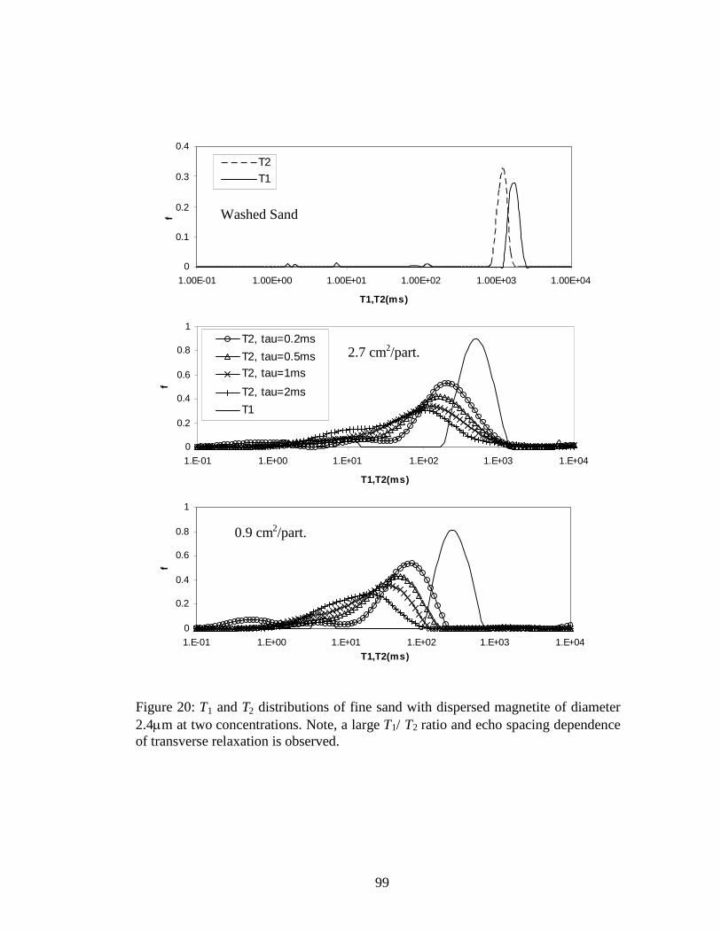
99
0
0.1
0.2
0.3
0.4
1.00E-01 1.00E+00 1.00E+01 1.00E+02 1.00E+03 1.00E+04
T1,T2(ms)
fT2T1
0
0.2
0.4
0.6
0.8
1
1.E-01 1.E+00 1.E+01 1.E+02 1.E+03 1.E+04
T1,T2(ms)
f
T2, tau=0.2ms
T2, tau=0.5msT2, tau=1ms
T2, tau=2ms
T1
0
0.2
0.4
0.6
0.8
1
1.E-01 1.E+00 1.E+01 1.E+02 1.E+03 1.E+04T1,T2(ms)
f
Figure 20: T1 and T2 distributions of fine sand with dispersed magnetite of diameter2.4m at two concentrations. Note, a large T1/ T2 ratio and echo spacing dependenceof transverse relaxation is observed.
0.9 cm2/part.
2.7 cm2/part.
Washed Sand
100
B.4 InterpretationThe diverse experimental results can be understood in terms of the characteristictime scales and relaxation regimes discussed in the previous section.
Motionally Averaging RegimeLet us first discuss the case of sand coated with ferric ions at differentconcentrations. Similar to ferric ions in solution, no echo spacing of transverserelaxation is observed. Also, the T1/T2 ratios of coated sand (1.24, 1.26 and 1.25for the three surface concentrations) are very close to the T1/T2 ratio of cleansand (1.26). The calculations of characteristic time scales (Table 1) show that therelaxation in the presence of angstrom size ferric ions is in motionally averagingregime. Thus, the secular relaxation is proportional to the square of theparamagnetic particle radius as postulated by outer sphere theory. Due to verysmall size of the paramagnetic ferric ion, the contribution of secular relaxation tothe transverse relaxation is negligible. Consequently, the T1/T2 ratio remainssame and no echo spacing dependence of T2 relaxation is observed forparamagnetic relaxation by ferric ions.
The argument of motionally averaging regime can be extended to explain therelaxation characteristics of sand coated with 25nm and 110nm magnetite at lowconcentrations. The constraint of low concentration ensures that the internalfields induced by neighboring paramagnetic particles do not superpose. Thus,the protons dephase as if diffusing in the inhomogeneous field induced by asingle paramagnetic particle. Figures 18 and 19 show that at low surfacecoverage of 25nm ( 49 10 nm2 ,104 nm2/particle) and 110nm (30 μm2 ,8μm2/particle), no echo spacing dependence of T2 relaxation is observed and theT1/T2 ratio is close to that of the respective aqueous dispersions. At these surfacecoverages, the interparticle distance is greater than 10 times the radius of theparticle and the internal fields induced by neighboring particles do not overlap.Thus, the length scale of field inhomogenity is determined by the size of theparamagnetic particle. Motionally averaging regime of secular relaxation isobserved and T2 relaxation shows no echo spacing dependence. Additionally,the T1/T2 ratio of coated sand increases with the particle size (1.2 for ferric ionsand 1.6 for 25nm particle). Thus, the earlier observation that the T1/T2 ratioincreases with particle size (Figure 14) is also verified for paramagnetic particlesadsorbed on sand surface.
Localization RegimeNow, let us analyze the results for the sand coated with high concentrations ofthe magnetite nanoparticles. At the highest surface coverage of 25nm( 33 10 nm2/particle) and 110nm particle (0.3 μm2/particle) in figures 8 and 9, anecho spacing dependence of T2 relaxation is observed. This is because at highsurface coverage, the particles form a ‘shell’ around each sand grain such thatthe length scale of the field inhomogenity becomes large compared to thediffusion length during the time of the echo spacing. Consider a sand grain of
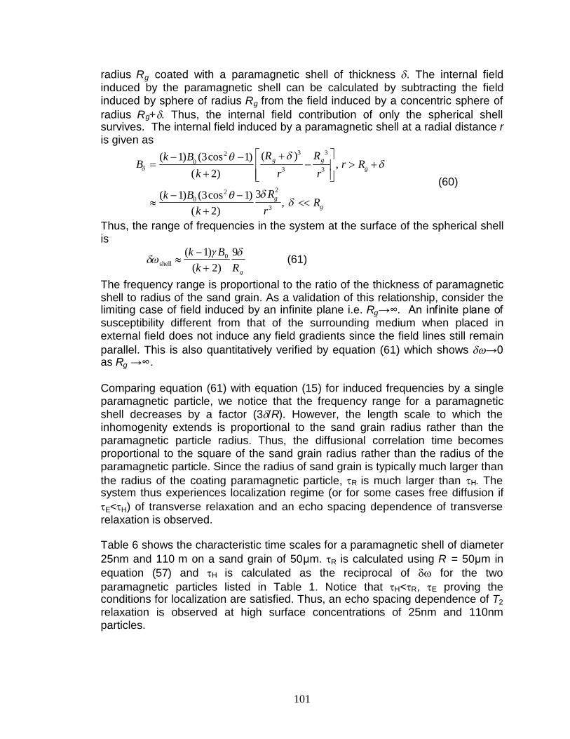
101
radius Rg coated with a paramagnetic shell of thickness . The internal fieldinduced by the paramagnetic shell can be calculated by subtracting the fieldinduced by sphere of radius Rg from the field induced by a concentric sphere ofradius Rg+. Thus, the internal field contribution of only the spherical shellsurvives. The internal field induced by a paramagnetic shell at a radial distance ris given as
3 320
3 3
220
3
( )( 1) (3cos 1),
( 2)
3( 1) (3cos 1),
( 2)
g gg
gg
R Rk BB r R
k r r
Rk BR
k r
(60)
Thus, the range of frequencies in the system at the surface of the spherical shellis
0shell
( 1) 9( 2) g
k Bk R
(61)
The frequency range is proportional to the ratio of the thickness of paramagneticshell to radius of the sand grain. As a validation of this relationship, consider thelimiting case of field induced by an infinite plane i.e. Rg→∞. An infinite plane of susceptibility different from that of the surrounding medium when placed inexternal field does not induce any field gradients since the field lines still remainparallel. This is also quantitatively verified by equation (61) which shows →0 as Rg →∞.
Comparing equation (61) with equation (15) for induced frequencies by a singleparamagnetic particle, we notice that the frequency range for a paramagneticshell decreases by a factor (3/R). However, the length scale to which theinhomogenity extends is proportional to the sand grain radius rather than theparamagnetic particle radius. Thus, the diffusional correlation time becomesproportional to the square of the sand grain radius rather than the radius of theparamagnetic particle. Since the radius of sand grain is typically much larger thanthe radius of the coating paramagnetic particle, R is much larger than H. Thesystem thus experiences localization regime (or for some cases free diffusion ifE<H) of transverse relaxation and an echo spacing dependence of transverserelaxation is observed.
Table 6 shows the characteristic time scales for a paramagnetic shell of diameter25nm and 110 m on a sand grain of 50μm. R is calculated using R = 50μm inequation (57) and H is calculated as the reciprocal of for the twoparamagnetic particles listed in Table 1. Notice that H<R, E proving theconditions for localization are satisfied. Thus, an echo spacing dependence of T2relaxation is observed at high surface concentrations of 25nm and 110nmparticles.

Localiparamrelaxacharac110nmand thshown
Regim
The eT1/T2(Kleinbdiffusiwith thof parcan resmallespacindepenimply
In sanparamBurba
Table 6: Characteristic time scales for relaxation in sandcoated with 25nm and 110nm magnetite at high surfaceconcentrations.
Time Scale (sec) 25nm 110nmR 1 1E,minimum
42 10 42 10
102
zation regime can also be observed for relaxation in the presence of largeagnetic particles with large diffusional correlation time. This is case fortion in sand with dispersed 2.4μm magnetite. The values of theteristic times are mentioned in Table 7. (is assumed to be same as forparticles). The conditions for localization regime (H<R, E) are satisfied
us, an echo spacing dependence of transverse relaxation is observed asin Figure 20.
es of paramagnetic relaxation in sandstones
xperimental results of figures 17, 18 and 19 explain the observed range ofratio in sandstones with no echo spacing dependence of T2 relaxationerg et al.,1993). In the motionally averaging regime, relaxation due to
on in inhomogeneous fields induced by paramagnetic particles increasese size and susceptibility of the paramagnetic particle. Thus, the presence
amagnetic minerals of various sizes and susceptibilities on pore surfacessult in a range of T1/T2 ratios. Since the diffusional correlation time is muchr than the time for echo formation in motionally averaging regime, no echog dependence of the T2 relaxation would be observed. The lack ofdence of transverse relaxation on echo spacing, thus, does not necessarilythat relaxation is not influenced by diffusion effects.
dstones, the localization regime can arise due to the presence of largeagnetic particles such as clays. An example of such a system is North-nk sandstone which has macropores lined with chlorite clay flakes. Zhang
Table 7: Characteristic time scales for relaxationin sand with dispersed 2.4μm magnetite
Time Scale (sec) 2.4μmR
46 10E,minimum
42 10H
610
H55.2 10 55 10

103
et al. (2003) modeled the gradients induced in a pore lined with clay flakes suchthat the flakes form micropores that open to a larger macropore. They found thatlarge field gradients are concentrated around the sharp corners of the clay flakesand in the micropores between clay flakes. The gradients also extendconsiderably in the macropore although the strength is not as high as inmicropores. Fluid molecules in the micropore and macropore are, however,coupled by diffusion (Anand et al., 2005). Thus, in general the moleculesexperience gradients that are intermediate to those in the micro and macropores.
Figure 21 shows the T1 and T2 distributions of two water-saturated North Burbanksandstone cores. The T2 distributions are shown as a function of echo spacings.Once again, a large T1/T2 ratio is observed and the T2 distributions show echospacing dependence. These observations are expected for the localizationregime of transverse relaxation in the presence of large internal field gradients.The logmean longitudinal and transverse relaxation times for the cores are listedin Table 8.
0
0.03
0.06
0.09
0.12
0.15
1.E-01 1.E+00 1.E+01 1.E+02 1.E+03 1.E+04
T1,T2(ms)
f
T2, tau=0.16msT2, tau=0.24msT2, tau=0.48msT2, tau=1T1
0
0.02
0.04
0.06
0.08
1.E-01 1.E+00 1.E+01 1.E+02 1.E+03 1.E+04
T1,T2(ms)
f
Figure 21: T1 and T2 distributions of water saturated North Burbank sandstonecores 1 and 2.
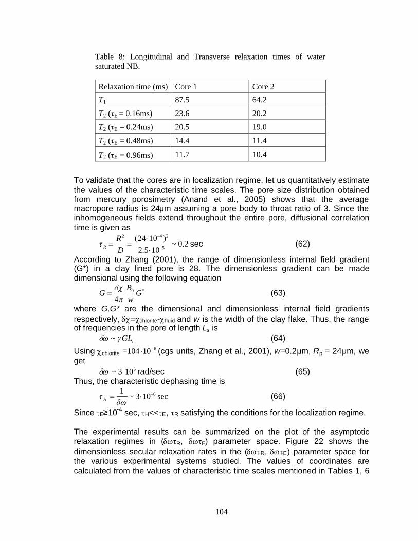
104
To validate that the cores are in localization regime, let us quantitatively estimatethe values of the characteristic time scales. The pore size distribution obtainedfrom mercury porosimetry (Anand et al., 2005) shows that the averagemacropore radius is 24μm assuming a pore body to throat ratio of 3. Since theinhomogeneous fields extend throughout the entire pore, diffusional correlationtime is given as
2 4 2
5
(24 10 )~ 0.2
2.5 10R
RD
sec (62)
According to Zhang (2001), the range of dimensionless internal field gradient(G*) in a clay lined pore is 28. The dimensionless gradient can be madedimensional using the following equation
*0
4B
G Gw
(63)
where G,G* are the dimensional and dimensionless internal field gradientsrespectively, =chlorite-fluid and w is the width of the clay flake. Thus, the rangeof frequencies in the pore of length Ls is
~ sGL (64)
Using chlorite = 6104 10 (cgs units, Zhang et al., 2001), w=0.2μm, Rp = 24μm, weget
5~ 3 10 rad/sec (65)Thus, the characteristic dephasing time is
61~ 3 10 secH
(66)
Since E≥10-4 sec, H<<E, R satisfying the conditions for the localization regime.
The experimental results can be summarized on the plot of the asymptoticrelaxation regimes in (R, E) parameter space. Figure 22 shows thedimensionless secular relaxation rates in the (R, E) parameter space forthe various experimental systems studied. The values of coordinates arecalculated from the values of characteristic time scales mentioned in Tables 1, 6
Table 8: Longitudinal and Transverse relaxation times of watersaturated NB.
Relaxation time (ms) Core 1 Core 2
T1 87.5 64.2
T2 (E = 0.16ms) 23.6 20.2
T2 (E = 0.24ms) 20.5 19.0
T2 (E = 0.48ms) 14.4 11.4
T2 (E = 0.96ms) 11.7 10.4

105
and 7. The corresponding experimental rates are normalized by a characteristicrate defined as
0
1f
t (67)
where f is the volume fraction of the paramagnetic particles. The values of f andused in the calculation are mentioned in Appendix A. For comparison, thecontours of dimensionless relaxation rates predicted by theoretical expressionsfor the three asymptotic regimes are also plotted. A good quantitative agreementbetween the theoretically predicted rates and experimentally measured rates isobserved for all cases.
The relaxation characteristics of the experimental systems in Figure 22 can beexplained in terms of the asymptotic regimes. The aqueous dispersions ofnanoparticles (open circles) and coated sand at low surface concentrations (opentraingles) fall in motionally averaging regime. Thus no echo spacing is observedand T1/T2 ratio increase with particle size. Experiments with sand coated at highconcentrations of 25nm (open inverted triangles) and 110nm (open squares) liein localization regime. Thus, an echo spacing dependence of the T2 relaxation isobserved. Similarly, North Burbank sandstone (solid circles) and sand withdispersed 2.4μm magnetite (solid diamonds) also fall in localization regime anddisplay an echo spacing dependence.

106
In figure 23 we plot the secular relaxation rates with the echo spacing for theseveral cases of localization regimes observed in figures 18-21. The solid linesrepresent linear fit between the relaxation rates and the echo spacing. As wasshown by the random walk simulations, the echo spacing dependence of secularrelaxation in the localization regime is almost linear and not quadratic. Theseresults thus explain the earlier observations of Brown et al. (1993) and Fantazziniet al. (2005) who found a quasi-linear dependence of transverse relaxation onthe echo spacing in porous media.
10-2 100 102 104 10610 -1
100
101
102
103
104
R
E
0.01 0.1
1
0.01
0.0001
1
0.010.0001
1e-006
0.08
0.63
0.130.040.01
0.03
0.04
0.06
0.1
0.0008
0.0006
0.00040.00030.007
0.004
0.002
0.001 0.0003
0.00040.00150.002
Figure 22: Parametric representation of experimentally measured secularrelaxation rates for various systems in the (R, E) parameter space. (Δ) aqueous dispersion of 4nm, 9nm, 16nm particles () sand coated with diluteconcentrations of 25nm and 110nm particles () sand coated with high surfaceconcentration of 25nm () sand coated with high surface concentration of 110nm,() sand with dispersed 2.4μm magnetite () North Burbank sandstone.

107
ConclusionsDiffusion of spins in magnetic field inhomogenities leads to additional transverserelaxation due to dephasing called secular relaxation. Random walk simulationsof proton relaxation in the presence of paramagnetic particles show that secularrelaxation is characterized by three time scales: diffusional correlation time (R),time for significant dephasing (H) and half echo spacing of the CPMG sequence(E). The smallest characteristic time determines the classification of secularrelaxation into three asymptotic regimes of motionally averaging, localization andfree diffusion. This classification of relaxation regimes using characteristic timescales is independent of the particular choice of inhomogeneous field distribution.
The asymptotic regimes show different relaxation characteristics. In themotionally averaging regime, field inhomogenities are averaged due to fastdiffusion in time much smaller than E. Thus, no echo spacing dependence oftransverse relaxation is observed. Additionally, the relaxation rate increases withthe length scale of field inhomogenity. In the free diffusion regime, secularrelaxation rate shows quadratic dependence on the echo spacing. However, thedependence on the length scale of inhomogenity is inversed and the relaxationrate decrease with the increase in size of the paramagnetic particle. This is
0.5 1 1.5 2 2.5 30
0.01
0.02
0.03
0.04
0.05
0.06
0.07
0.08
tau (ms)
1/T
2,se
c
2.4m, C=2.7cm2/part.2.4m, C=0.9cm2/part.25nm, C=3.103nm2/part.North Burbank, Core 1
Figure 23: Plot of secular relaxation rates with echo spacing for different cases oflocalization regime. The solid lines are the linear best fits of the experimentalpoints.

108
because the average gradient decreases with the increase in particle size. In thelocalization regime, relaxation rate shows a quasi- or sub-linear dependence onecho spacing. The dependence on field inhomogenity length scale is inversed.The characteristics of the relaxation regimes can be demonstrated in a singlecontour map of dimensionless relaxation rate in (R/H, E/H) parameter space.
The relaxation characteristics of asymptotic regimes can also provide explanationfor the diverse NMR characteristics observed in fluid-saturated sandstones. Alarge range of T1/T2 ratio in sandstones with no echo spacing dependence of T2
relaxation observed by Kleinberg et al. (1993) can arise in the motionallyaveraging regime. The quasi or sub-linear dependence of the T2 relaxation onecho spacing shown in the experiments of Zhang et al. (2001) and Brown et al.(1995) can arise in the localization regime. Thus, the calculation of characteristictime scales can provide a quantitative understanding of paramagnetic relaxationin sandstones.
References:
1) Agarwal, S., 2007, Ph.D. Thesis, Rice University.2) Anand, V. and Hirasaki, G.J., 2005, “Diffusional Coupling between micro
and macropores for NMR relaxation in Sandstones and Carbonates”,Proceedings of the 46th Annual SPWLA symposium, New Orleans, LA.
3) Bertini, I., Capozzi, F., Luchinat, C. and Xia, Z., 1993, “Nuclear andElectron Relaxation in Fe(OH2)6
3+, Journal of Physical Chemistry, 97, p1134-1137.
4) Brooks,R.A., Moiny F. and Gillis,P., 2001, “On T2 Shortening by WeaklyMagnetized Particles: The Chemical Exchange Model”, MagneticResonance in Medicine, Vol 45, p 1014-1020.
5) Brown, R.J.S. and Fantazzini, P., 1993, “Conditions for initial quasilinear1
2T versus for Carr-Purcell-Meiboom-Gill NMR with diffusion andsusceptibility differences in porous media and tissues”, Physical Review B,47, 22, p14823-14834.
6) Carr,H.Y. and Purcell, E.M., 1954, “Effects of Diffusion on FreePrecession in Nuclear Magnetic Resonance Experiments”, PhysicalReview, Vol 94, No 3, p 630-638.
7) DeSwiet, T.M and Sen, P., 1993, “Decay of nuclear magnetization bybounded diffusion in a constant field gradient”, Journal of ChemicalPhysics, Vol 100, No 8, p 5597-5604.
8) Fantazzini, P and Brown, R.J.S, 2005, “Initially linear echo-spacingdependence of 1/T2 measurements in many porous media with pore scaleinhomogeneous fields”, Journal of Magnetic Resonance,Vol 17, p 228-235.
9) Gillis, P. and Koenig, S.H., 1987, “Transverse relaxation of SolventProtons Induced by Magnetized Spheres: Application to Ferritin,Erythrocytes and Magnetite”, Magnetic Resonance in Medicine, Vol 5,p323-345.
109
10)Gillis, P., Moiny,F. and Brooks, R.A., 2002, “On T2-Shortening by stronglymagnetized spheres: a partial refocusing model”, Magnetic Resonance inMedicine, Vol 34,p 227-233.
11)Jenson,J.H. and Chandra, R., 2000, “NMR Relaxation in Tissues withWeak Magnetic Inhomogeneities”, Magnetic Resonance in Medicine, Vol44, p144-156.
12)Kleinberg, R.L. and Farooqui, S.A., 1993, “T1/T2 ratio and frequencydependence of NMR Relaxation in Porous Sedimentary Rocks”, Journal ofColloid and Interface Science, 158, p195-198.
13)Kleinberg, R.L., Kenyon, W.E. and Mitra, P.P., 1994, “Mechanism of NMRRelaxation of Fluids in Rocks”, Journal of Magnetic Resonance Series A,108, p 206-214.
14)Lide, D.R., 1990-1991, “Handbook of Chemistry and Physics”, CRC Press,71st Edition.
15)Massart, R., 1981, “Preparation of Aqueous Magnetic Liquids in Alkalineand Acidic Media”, IEEE Transactions on Magnetics, 17 (2), p 1247-1248.
16)Menzel, D.A., “Fundamental Formulas of Physics”, Prentice Hall, NewYork, NY, 1955.
17)Morgan,L.O and Nolle, A.W., 1959, “Proton Spin Relaxation in AqueousSolutions of Paramagnetic Ions II. Cr+++,Mn++,Ni++,Cu++ and Gd+++, Journalof Chemical Physics, 31(2), p 365-368.
18)Neuman, C.H., 1974, “Spin echo of spins diffusing in a boundedmedium”,Journal of Chemical Physics, Vol 60,No. 11, p 4508-4511.
19)Sen, P.N., André,A and Axelrod,S, 1999, “Spins echoes of nuclearmagnetization diffusing in a constant magnetic field gradient and in arestricted geometry”, Journal of Chemical Physics,Vol 111,No. 14, p.6548-6555.
20)Solomon, I., 1955, “Relaxation Processes in a System of Two Spins”,Physical Review, 99(2), p 559-565.
21)Tarczon, J.C. and Halerpin, W.P., 1985, “Interpretation of NMR Diffusionmeasurements in uniform and nonuniform field gradients”, PhysicalReview B., Vol 32 (5), p2798-2807.
22)Weisskoff,R.M.,Zuo,C.S.,Boxerman,J.L. and Rosen,B.R., 1994,“Microscopic Susceptibility Variation and Transverse Relaxation: Theoryand Experiment”, Magnetic Resonance in Medicine, Vol 31, p 601-610.
23)Yu,W.W., Joshua, C., Yavuz, C.T. and Colvin, V.L., 2004, “Synthesis ofmonodisperse iron oxide nanocrystals by thermal decomposition of ironcarboxylate salts, Chemical Communication, web published on 2nd Sept2004.
24)Zhang, Q, 2001, “NMR Formation Evaluation: Hydrogen Index, Wettabilityand Internal Field Gradients”, Ph.D. Thesis, Rice University.
25)Zhang, G.Q., Hirasaki, G.J., House, W.V., 2003, “Internal field gradients inporous media”, Petrophysics, 42, p422-434.
26)Zhang, G.Q and Hirasaki,G.J., 2003, “CPMG relaxation by diffusion withconstant magnetic field gradient in a restricted geometry: numerical

110
simulation and application”, Journal of Magnetic Resonance, Vol 163, p81-91.
Appendix Af is the volume fraction of the paramagnetic particles. The values of f are easilydetermined for the different cases. For the case of aqueous dispersion of theparticles, f is given as
Cfd
(A1)
where C is the concentration of the dispersion (g/ml). Magnetite density(d=5.18g/cm3) is obtained from Lide et al. (CRC Press). For nanoparticleadsorbed on silica surface at low concentrations, f is given by the quantity ofadsorbed paramagnetic material divided by magnetite density and pore volume.At high concentrations, f is approximately the solid matrix volume fraction sincethe particles are assumed to be forming a shell around sand grains. For NorthBurbank core, f (=0.3) is obtained from the volumetric calculations of micro andmacropore done by Zhang et al. (2001).
Table A1: f and used for the computation of dimensionless relaxation rates for thevarious experimental systems.
25nm104 , 49 10 nm2/part.
110nm0.3, 8 cm2/part.
2.4μm2.7, 0.9cm2/part
NorthBurbank
f(dimensionless)
42 10 , 51 10 42 10 , 54 10 4 41.3 10 ,4 10 0.3
(rad/sec) 64 10 610 610 53 10
Task 3: Characterization of pore structure and wettability
NMR Well Logging and Special Core Analysis for
Fluid-Rock Characterization
Subcontract to Rice University on
DOE Award Number: DE-PS26-04NT15450-2C
Semi-Annual Report
Reporting Period Start Date: 4-1-2005
Reporting Period End Date: 9-30-2006
I. Tripathi, R. Pitchumani, & K. K. Mohanty
Oct 2006
University of Houston
4800 Calhoun Road
Houston, TX 77204-4004

112
Abstract
Characterization of pore structure and wettability has been completed on six carbonate
samples. The vug size, distribution and interconnection vary significantly in these six
samples. The thin sections have been characterized through their pore size distribution,
two-point correlation function, chord number distribution, lineal path function and fractal
dimension. The power spectrum from Fourier transform has been computed. The three-
dimensional pore structures have been reconstructed for two carbonates and one
sandstone sample. Single phase permeability and NMR response has been measured for
all the samples. The relative permeability, NMR response and electrical conductivity
have been measured for three samples.
113
TABLE OF CONTENTS
Page
Cover Page 111
Abstract 112
Table of Contents 113
Introduction 114
Experimental Results 115
Conclusions 192

114
I. Introduction
The goal of this research is to relate NMR measurements in a core to its pore structure
and wettability and thus to permeability and relative permeability. In Task 3, 2D pore
structures will be extracted from thin-sections. The oil/brine/rock compositions will be
related to wettability as determined by contact angle goniometry and atomic force
microscopy. Amott wettability will be measured to define core scale wettability. Brine
and oil NMR response of the cores will be measured. NMR response of surfactant
solution imbibed carbonate cores will also be measured. NMR response will be simulated
from pore images and wettability. Mechanistic correlations will be developed between
NMR response, wettability and pore structure. Such correlation will help NMR logging
define the variation of pore structure and wettability through all logged wells.
In Task 4, NMR response will be related to permeability and relative permeabilities.
Such a correlation can estimate the reservoir heterogeneity and multiphase flow in logged
but non-cored wells. The relative permeability functions determine the time for water
breakthrough and the rate of oil recovery. Water-oil imbibition relative permeability will
be measured for each core plug. Electrical conductivity will be measured at end-point
saturations. Pore network models developed in Task 3 will be used to estimate the
relative permeabilities and electrical conductivity. Correlations will be made among the
NMR response and transport properties. Simple, but mechanistic correlations will be
developed for NMR response, permeability and relative permeability.
The project started in the last quarter of 2004. We have worked on four subtasks: pore
structure, wettability, NMR response and relative permeability/electrical conductivity of
six carbonate cores. The activities are described in the next section.
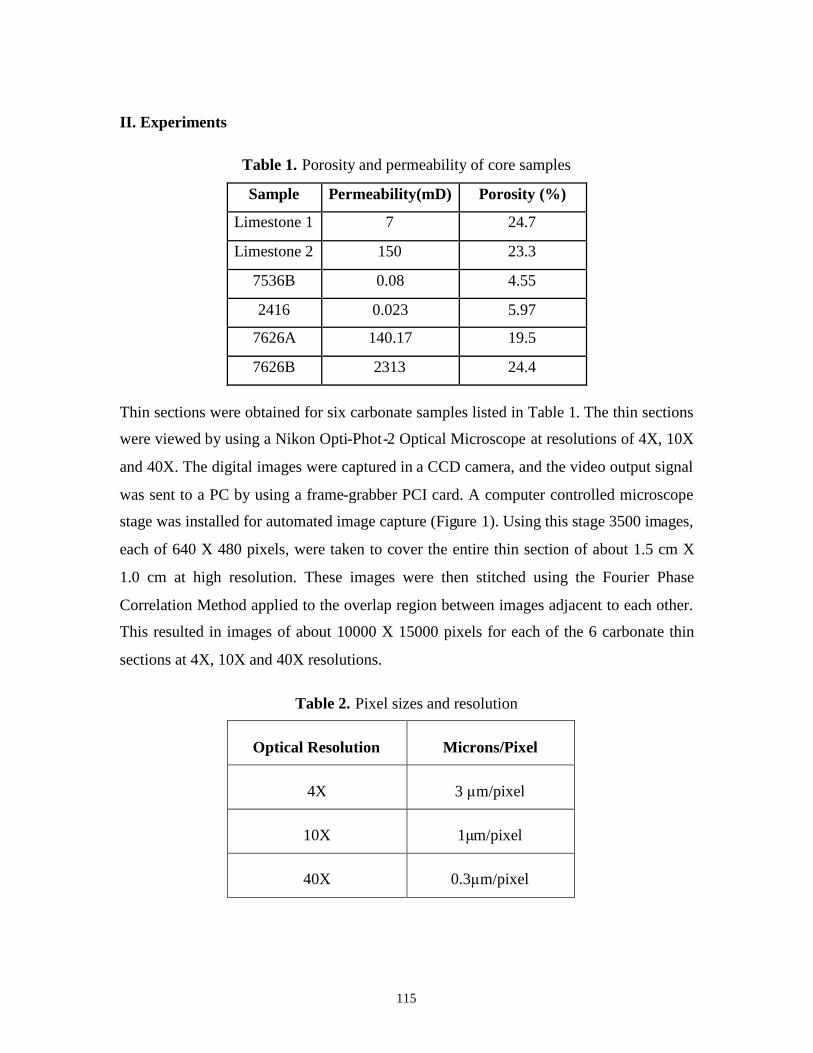
115
II. Experiments
Table 1. Porosity and permeability of core samples
Sample Permeability(mD) Porosity (%)
Limestone 1 7 24.7
Limestone 2 150 23.3
7536B 0.08 4.55
2416 0.023 5.97
7626A 140.17 19.5
7626B 2313 24.4
Thin sections were obtained for six carbonate samples listed in Table 1. The thin sections
were viewed by using a Nikon Opti-Phot-2 Optical Microscope at resolutions of 4X, 10X
and 40X. The digital images were captured in a CCD camera, and the video output signal
was sent to a PC by using a frame-grabber PCI card. A computer controlled microscope
stage was installed for automated image capture (Figure 1). Using this stage 3500 images,
each of 640 X 480 pixels, were taken to cover the entire thin section of about 1.5 cm X
1.0 cm at high resolution. These images were then stitched using the Fourier Phase
Correlation Method applied to the overlap region between images adjacent to each other.
This resulted in images of about 10000 X 15000 pixels for each of the 6 carbonate thin
sections at 4X, 10X and 40X resolutions.
Table 2. Pixel sizes and resolution
Optical Resolution Microns/Pixel
4X 3 μm/pixel
10X 1μm/pixel
40X 0.3μm/pixel

116
Figure 1. Imaging apparatus
Figure 2. Color image to B/W image conversion
The phase correlation method is described for cylindrically shifted images. Let g1
and g2 be the overlapping sections of images to be stitched and their respective Fourier
transforms be G1 and G2. Then the phase correlation is defined as

117
1 2( )1
( )
{ }
( ) ( ) j
i
i fj j
d F ewhere
G f G f e
For images shifted by a vector L
,
2 1( ) ( )g r g r L
and
2 .2 1( ) ( ) i f LG f G f e
.
The cross-correlation function d is a delta function given by
( )d r L
.
Thus the exact L
can be found by using the cross-correlation function d. This d is
calculated as a function of the position of g2 with respect to g1. At near perfect alignment
d is maximized. After the alignment, the images can be stitched in sequence to form a
composite image. An efficient code was developed in MATLAB based on this method
for stitching 3000 images.
Image segmentation is done on the composite images to convert them into a black
and white image with pores as white and rock as black (Figure 2). This binary image can
be analyzed for properties of the pore space described below.
2.1 Pore size distribution
Using erosion dilation algorithm we can identify each object in the pore space and
calculate its area (in pixels), and a number of other characteristics like the diameter of the
largest circle that can be fit completely inside that pore (called minimum diameter).
Figure 3-14 show the percentage of pore space area associated with pores of a particular
minimum diameter at the resolution of 1 μm/pixel for the horizontal and vertical thin
sections of each of the six carbonate samples.

118
Figure 3. Pore Size Distribution for Limestone 1 Horizontal Thin-Section
Figure 4. Pore Size Distribution for Limestone 1 Vertical Thin-Section

119
Figure 5. Pore Size Distribution for Limestone 2 Horizontal Thin-Section
Figure 6. Pore Size Distribution for Limestone 2 Vertical Thin-Section

120
Figure 7. Pore Size Distribution for 7536B Horizontal Thin-Section
Figure 8. Pore Size Distribution for 7536B Vertical Thin-Section

121
Figure 9. Pore Size Distribution for 2416 Horizontal Thin-Section
Figure 10. Pore Size Distribution for 2416 Vertical Thin-Section
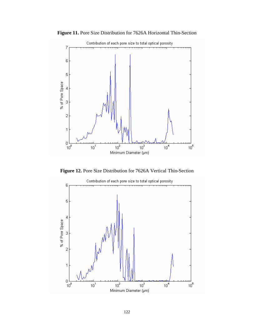
122
Figure 11. Pore Size Distribution for 7626A Horizontal Thin-Section
Figure 12. Pore Size Distribution for 7626A Vertical Thin-Section

123
Figure 13. Pore Size Distribution for 7626B Horizontal Thin-Section
Figure 14. Pore Size Distribution for 7626B Vertical Thin-Section

124
The pore size distributions of vuggy carbonates show that most of the porosity of the
sample is due to vugs in the size range of about 0.5 to 1 mm.. The packstones on the other
hand have a well distributed porosity with a mean pore size of about 30 microns.
2.2 Porosity
The binary image is equivalent to a discrete phase function Z(x) defined as
( )
( )
1( )
0p o r e
r o c kZ x
.
The porosity (Φ) is then defined as the statistical average
( )Z x .
The optical porosity of the thin section samples is dependent on the resolution of the
image and the amount of micro-porosity present in the sample. If the sample has vugs
then the optical porosity can even be greater than that of the whole core sample.
2.3 Autocorrelation function
The spatial autocorrelation function S2(r) is defined as the probability that two points at
the distance r both lie in the pore phase when randomly selected from the image. This can
be normalized by a function of porosity so that value of S2(r) ranges from 0 to 1. This
normalized autocorrelation function is given by
2 2
( ) ( )( )
Z x Z Z x r ZS r
For an isotropic system without long range order
2
2
(0) 1
lim ( ) 0r
S
S r
Also for a digitized 2D medium
2
0
( )4
r
dS r sdr
Where s = specific surface of the pore phase. Figure 15-26 show the two-point auto-
correlation function for the six limestone samples at a resolution of 1 μm/pixel. The
autocorrelation is calculated for both the horizontal and vertical sections along two
perpendicular directions named X and Y.

125
Figure 15. Two Point Autocorrelation Function for Limestone 1 Horizontal Thin Section
Figure 16. Two Point Autocorrelation Function for Limestone 1 Vertical Thin Section

126
Figure 17. Two Point Autocorrelation Function for Limestone 2 Horizontal Thin Section
Figure 18. Two Point Autocorrelation Function for Limestone 2 Vertical Thin Section
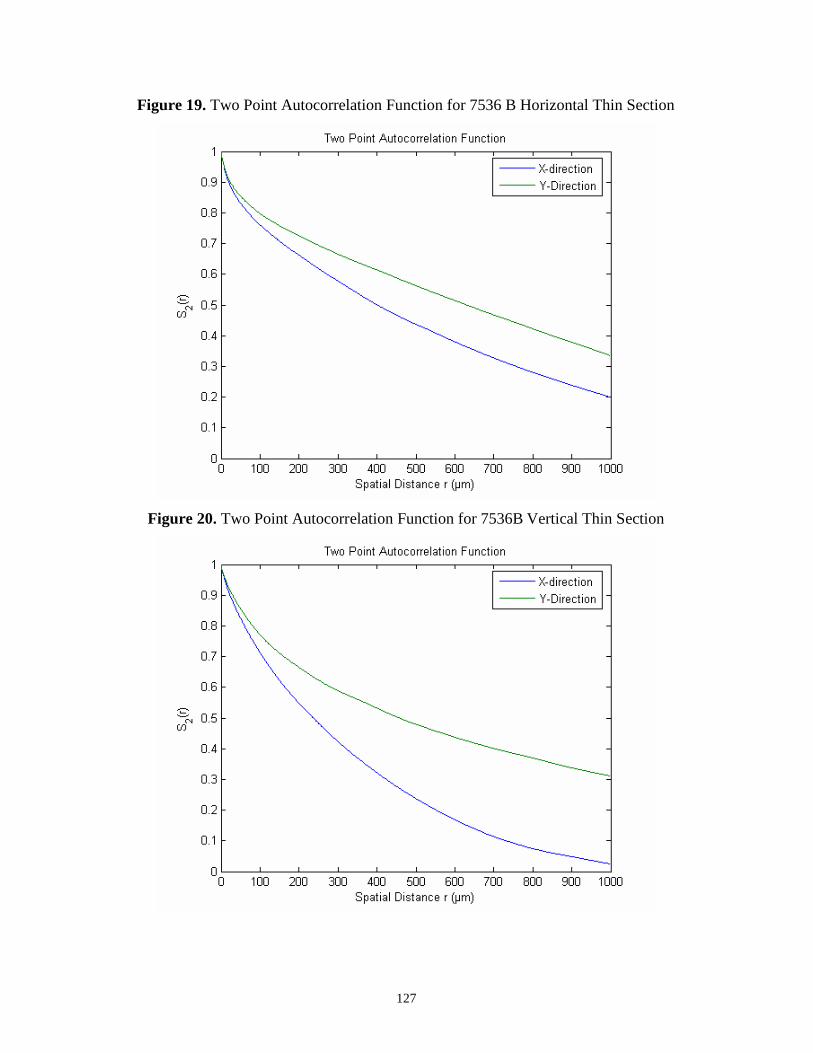
127
Figure 19. Two Point Autocorrelation Function for 7536 B Horizontal Thin Section
Figure 20. Two Point Autocorrelation Function for 7536B Vertical Thin Section

128
Figure 21. Two Point Autocorrelation Function for 2416 Horizontal Thin Section
Figure 22. Two Point Autocorrelation Function for 2416 Vertical Thin Section

129
Figure 23. Two Point Autocorrelation Function for 7626A Horizontal Thin Section
Figure 24. Two Point Autocorrelation Function for 7626A Vertical Thin Section

130
Figure 25. Two Point Autocorrelation Function for 7626B Horizontal Thin Section
Figure 26. Two Point Autocorrelation Function for 7626B Vertical Thin Section

131
It is interesting to note that the two-point autocorrelation function does not go to zero at 1
mm distance for vuggy sample which indicates long range spatial correlations. On the
other hand packstone samples show a correlation length of about 100μm.
2.4 Lineal Path Function
The lineal path function for the pore phase L(r) is defined as the probability of finding a
line segment of length r entirely in the pore space when randomly thrown into the image.
This is equivalent to the probability that a point can move a distance r along a direction
without crossing phase boundary between rock and pore. Figure 27-39 show the Lineal
path function for the six carbonate samples. The lineal paths are measured in two
perpendicular directions named X and Y for the horizontal and vertical section for each
sample at a resolution of 1 μm/pixel.
Figure 27. Lineal Path Function for Limestone 1 Horizontal Thin Section

132
Figure 28. Lineal Path Function for Limestone 1 Vertical Thin Section
Figure 29. Lineal Path Function for Limestone 2 Horizontal Thin Section

133
Figure 30. Lineal Path Function for Limestone 2 Vertical Thin Section
Figure 31. Lineal Path Function for 7536B Horizontal Thin Section
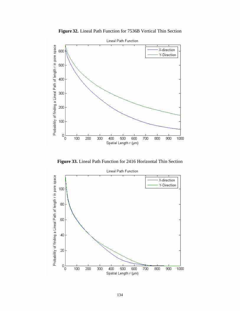
134
Figure 32. Lineal Path Function for 7536B Vertical Thin Section
Figure 33. Lineal Path Function for 2416 Horizontal Thin Section

135
Figure 34. Lineal Path Function for 2416 Vertical Thin Section
Figure 35. Lineal Path Function for 7626A Horizontal Thin Section
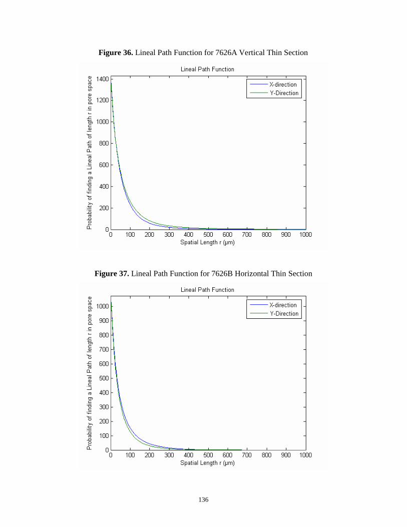
136
Figure 36. Lineal Path Function for 7626A Vertical Thin Section
Figure 37. Lineal Path Function for 7626B Horizontal Thin Section

137
Figure 38. Lineal Path Function for 7626B Vertical Thin Section
2.5 Chord Length Distribution Function
Chord length probability distribution function for pore space, p(r), is defined such that
p(r)dr is the probability of finding a chord of length between r and r + dr in pore space.
The mean chord length is the first moment of this probability distribution function given
by
0
( )cl rp r dr
In general, for statistically isotropic systems2
2
( )( ) cl d L rp rdr
Figure 39-50 show the chord length distribution function for all the carbonate samples for
the horizontal and vertical sections at a resolution of 1 μm/pixel. These are measured in
two perpendicular directions named X and Y.

138
Figure 39. Chord Number Distribution for Limestone 1 Horizontal Thin Section
Figure 40. Chord Number Distribution for Limestone 1 Vertical Thin Section

139
Figure 41. Chord Number Distribution for Limestone 2 Horizontal Thin Section
Figure 42 Chord Number Distribution for Limestone 2 Vertical Thin Section
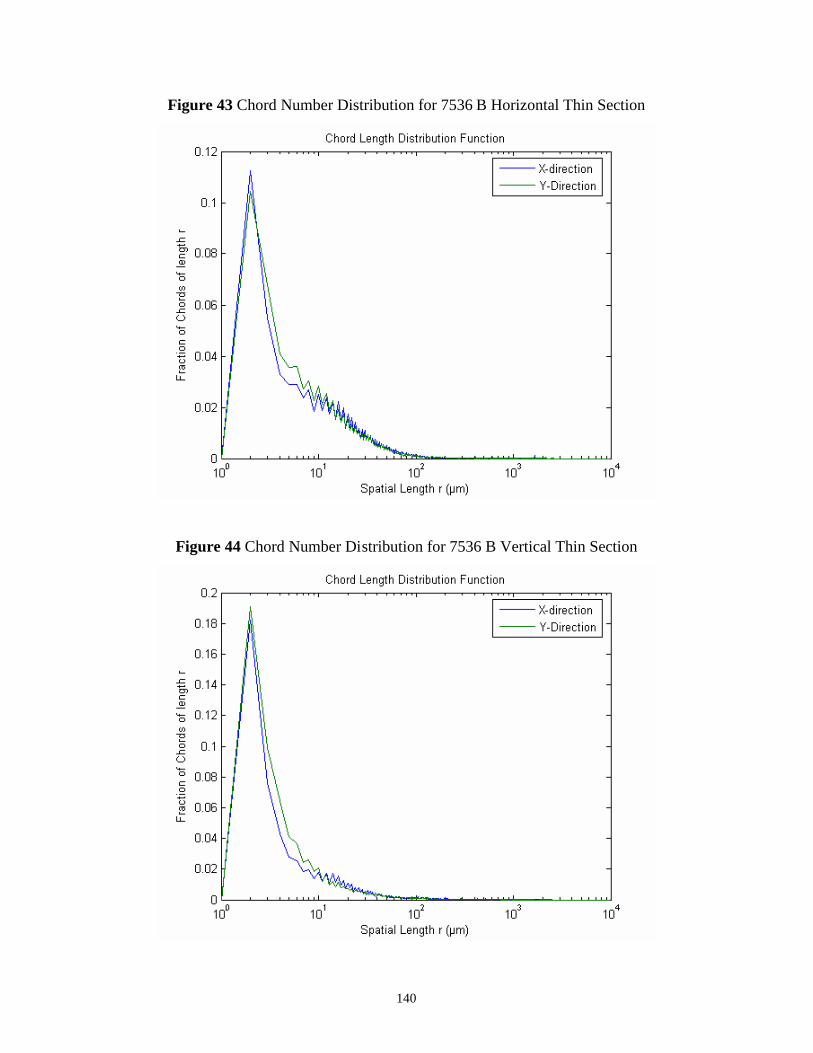
140
Figure 43 Chord Number Distribution for 7536 B Horizontal Thin Section
Figure 44 Chord Number Distribution for 7536 B Vertical Thin Section

141
Figure 45 Chord Number Distribution for 2416 Horizontal Thin Section
Figure 46 Chord Number Distribution for 2416 Vertical Thin Section

142
Figure 47 Chord Number Distribution for 7626A Horizontal Thin Section
Figure 48 Chord Number Distribution for 7626A Vertical Thin Section

143
Figure 49 Chord Number Distribution for 7626B Horizontal Thin Section
Figure 50 Chord Number Distribution for 7626B Vertical Thin Section

144
2.6 Fourier Transform
In the mechanism of grain deposition and subsequent diagenesis, the grains compact well
to form clusters with the flaws between clusters providing the channels for flow. These
channels can be differentiated from an inter-granular pore in a 2-D image using radial
power spectrum derived from Fourier transform which gives a characteristic peak
associated with grain size and another associated with the grain clusters at about 1.2
times the grain peak. A filter based on the power spectrum can then be used to distinguish
between the two types of porosities. Figure 51 shows the radial power spectrum of a
sample of Berea sandstone.
Figure 51 Radial Power Spectrum for Berea Sandstone
Since a carbonate undergoes drastic changes during diagenesis, the original grain
deposition pattern is altered. In general for the carbonate samples studied, the peak is not
as sharp as in the case of sandstones indicating absence of a dominant grain size. Figures
52-63 show the radial power spectrum for the six sandstone samples for the horizontal
and vertical sections.

145
Figure 52. Radial Power Spectrum for Limestone 1 Horizontal Section
Figure 53. Radial Power Spectrum for Limestone 1 Vertical Section

146
Figure 54. Radial Power Spectrum for Limestone 2 Horizontal Section
Figure 55. Radial Power Spectrum for Limestone 2 Vertical Section
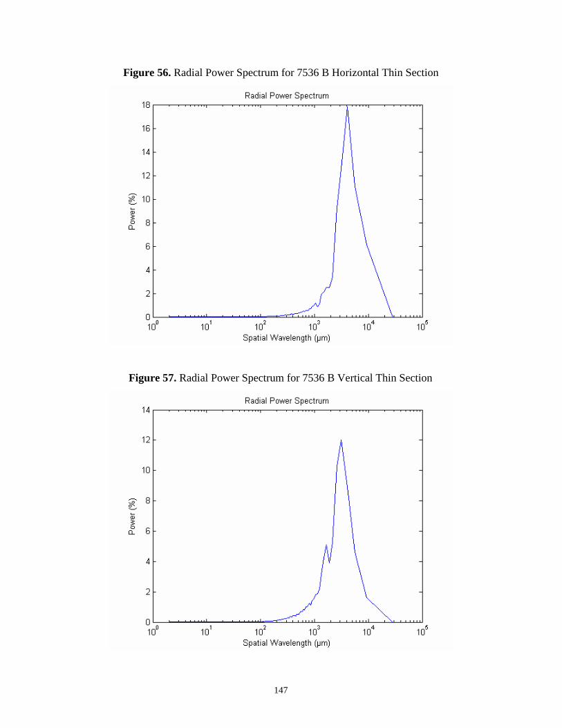
147
Figure 56. Radial Power Spectrum for 7536 B Horizontal Thin Section
Figure 57. Radial Power Spectrum for 7536 B Vertical Thin Section

148
Figure 58. Radial Power Spectrum for 2416 Horizontal Thin Section
Figure 59. Radial Power Spectrum for 2416 Vertical Thin Section

149
Figure 60. Radial Power Spectrum for 7626A Horizontal Thin Section
Figure 61. Radial Power Spectrum for 7626A Vertical Thin Section
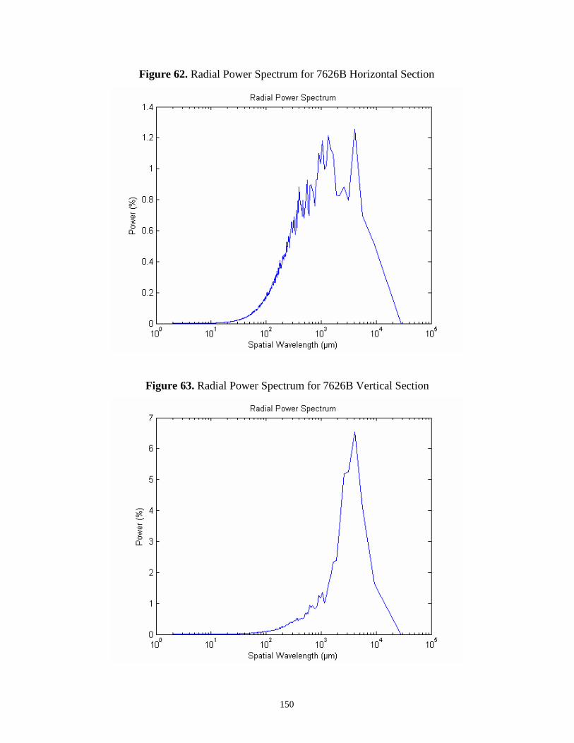
150
Figure 62. Radial Power Spectrum for 7626B Horizontal Section
Figure 63. Radial Power Spectrum for 7626B Vertical Section

151
2.7 Fractal Dimension
The fractal dimension of each set of images is calculated using the box counting method.
Three different types of features in an image are studied – the fraction of image occupied
rock, the fraction of image occupied by pore and the fraction of image having the
interface between rock and pore. The fractal dimensions are calculated by counting the
number of boxes containing the respective feature F and plotting the box count vs box
size. The fractal dimension is given by
log( ( ))log( )
B
B
N FD
L
where D is the fractal dimension for feature F, Nb is the number of boxes of size Lb which
contain the feature F. In the following figures Dm is the fractal dimension of the matrix,
Dp is the fractal dimension of the pore space and Ds is the fractal dimension of the
interface between pore and rock. Figures 64 – 99 show the fractal dimension calculation
and values for matrix, pore and surface dimensions for the horizontal and vertical section
of 6 carbonate samples at a resolution of 1 μm/pixel.
Figure 64 Matrix Fractal Dimension for Limestone 1 Horizontal Section

152
Figure 65 Pore Space Fractal Dimension for Limestone 1 Horizontal Section
Figure 66 Surface Fractal Dimension for Limestone 1 Horizontal Section
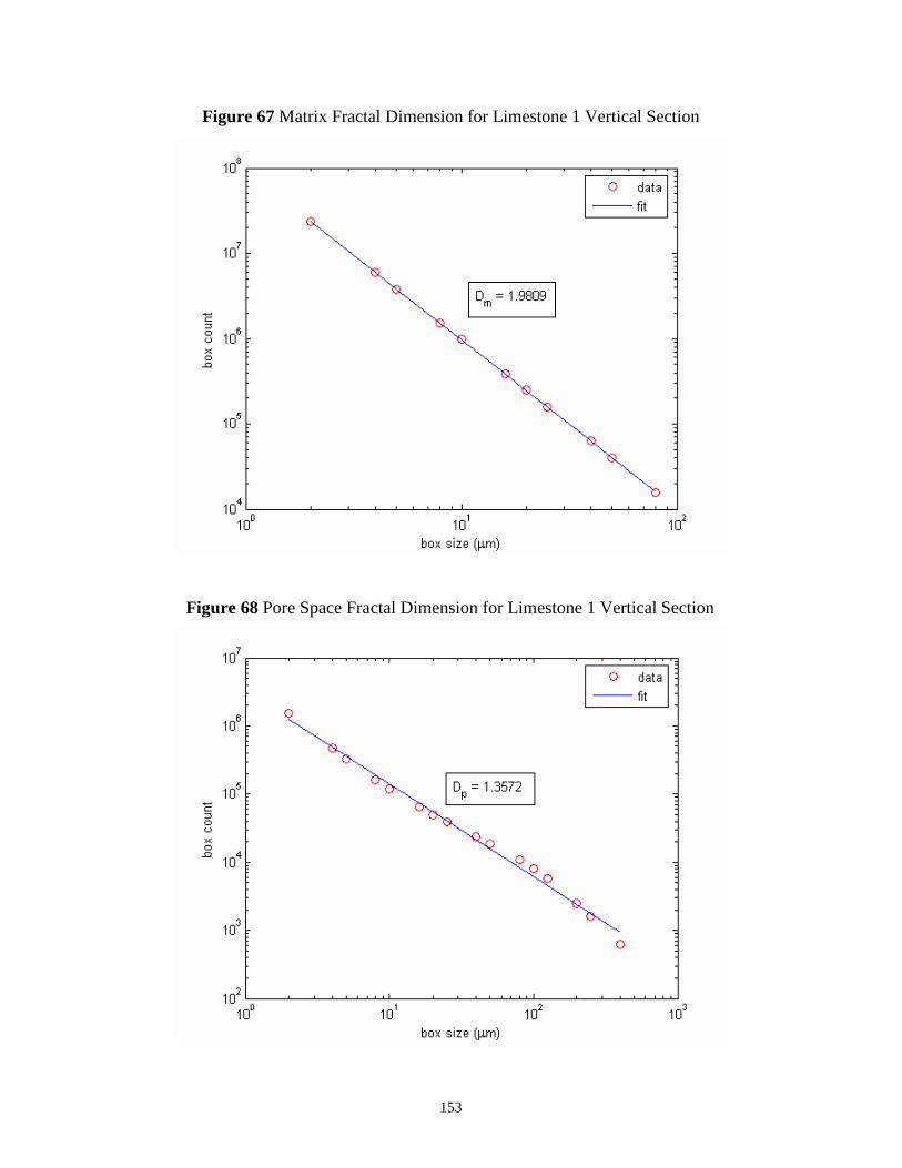
153
Figure 67 Matrix Fractal Dimension for Limestone 1 Vertical Section
Figure 68 Pore Space Fractal Dimension for Limestone 1 Vertical Section

154
Figure 69 Surface Fractal Dimension for Limestone 1 Vertical Section
Figure 70 Matrix Fractal Dimension for Limestone 2 Horizontal Section
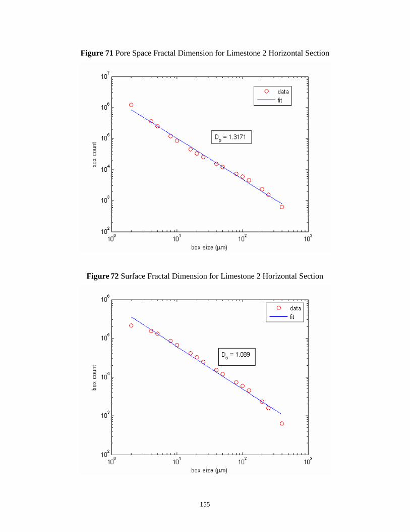
155
Figure 71 Pore Space Fractal Dimension for Limestone 2 Horizontal Section
Figure 72 Surface Fractal Dimension for Limestone 2 Horizontal Section
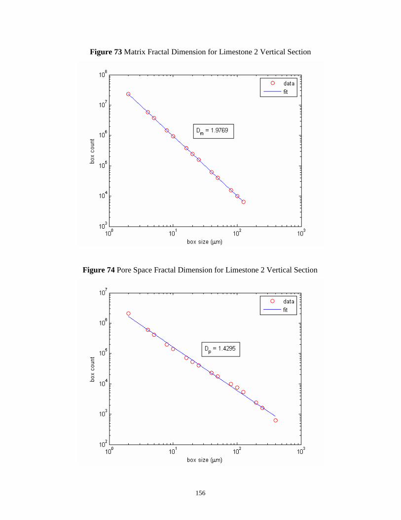
156
Figure 73 Matrix Fractal Dimension for Limestone 2 Vertical Section
Figure 74 Pore Space Fractal Dimension for Limestone 2 Vertical Section

157
Figure 75 Surface Fractal Dimension for Limestone 2 Vertical Section
Figure 76 Matrix Fractal Dimension for 7536 B Horizontal Section

158
Figure 77 Pore Space Fractal Dimension for 7536 B Horizontal Section
Figure 78 Surface Fractal Dimension for 7536 B Horizontal Section
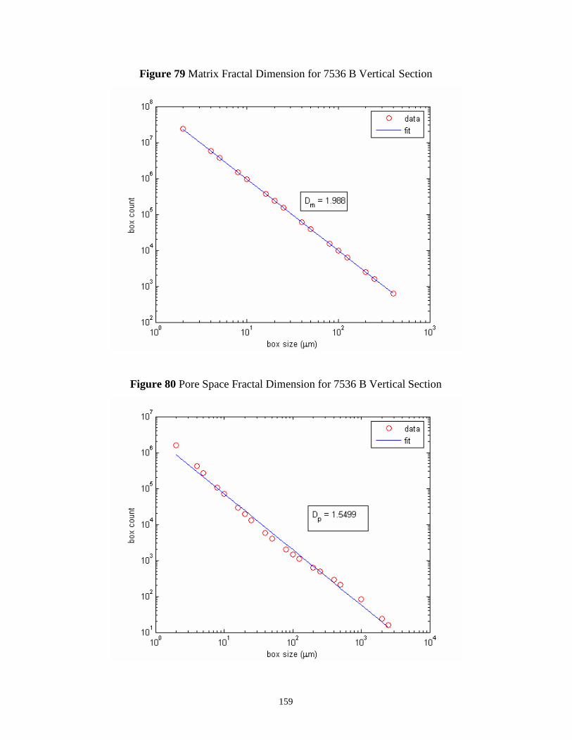
159
Figure 79 Matrix Fractal Dimension for 7536 B Vertical Section
Figure 80 Pore Space Fractal Dimension for 7536 B Vertical Section

160
Figure 81 Surface Fractal Dimension for 7536 B Vertical Section
Figure 82 Matrix Fractal Dimension for 2416 Horizontal Section
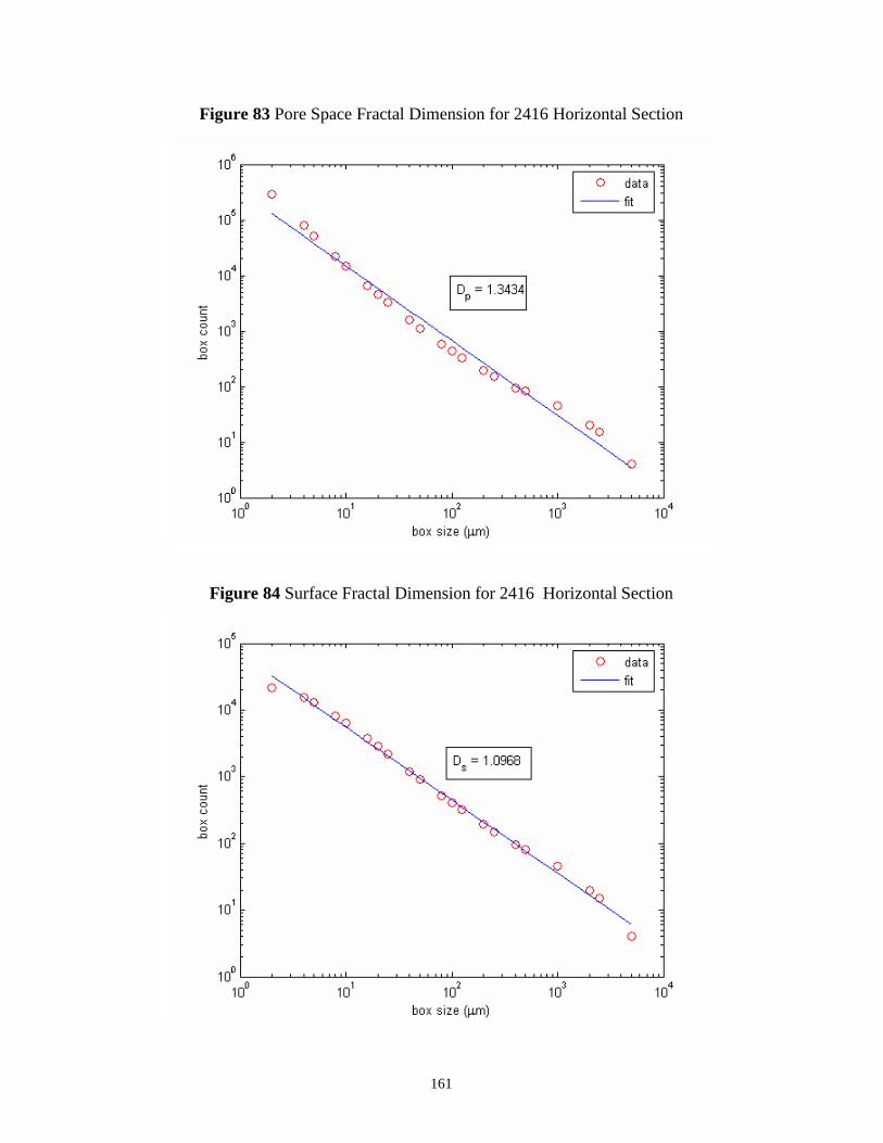
161
Figure 83 Pore Space Fractal Dimension for 2416 Horizontal Section
Figure 84 Surface Fractal Dimension for 2416 Horizontal Section

162
Figure 85 Matrix Fractal Dimension for 2416 Vertical Section
Figure 86 Pore Space Fractal Dimension for 2416 Vertical Section
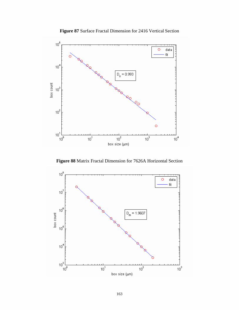
163
Figure 87 Surface Fractal Dimension for 2416 Vertical Section
Figure 88 Matrix Fractal Dimension for 7626A Horizontal Section

164
Figure 89 Pore Space Fractal Dimension for 7626A Horizontal Section
Figure 90 Surface Fractal Dimension for 7626A Horizontal Section
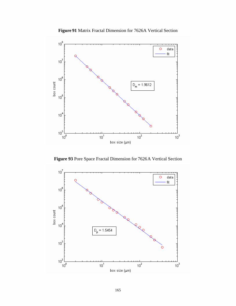
165
Figure 91 Matrix Fractal Dimension for 7626A Vertical Section
Figure 93 Pore Space Fractal Dimension for 7626A Vertical Section

166
Figure 93 Surface Fractal Dimension for 7626A Vertical Section
Figure 94 Matrix Fractal Dimension for 7626B Horizontal Section

167
Figure 95 Pore Space Fractal Dimension for 7626B Horizontal Section
Figure 96 Surface Fractal Dimension for 7626B Horizontal Section

168
Figure 97 Matrix Fractal Dimension for 7626B Vertical Section
Figure 98 Pore Space Fractal Dimension for 7626B Vertical Section

169
Figure 99 Surface Fractal Dimension for 7626B Vertical Section
2.8 3-D Reconstruction
The procedure of simulated annealing has been used to reconstruct 3-D porous media
from 2-D sections. In this procedure, the statistical functions described in sections 2.2-2.5
are calculated for a thin section image. Then a random 3-D structure is constructed so that
it has the same porosity as given by the thin section. The same statistical functions are
calculated for the 3-D structure and the procedure involves evolving the structure using
simulated annealing so that its statistical properties are closer to that from the 2-D image.
For the functions 0 ( ); [1, ]if r i n from the 2-D image, it is assumed that they are
independent of the direction of r so that they can be applied to the reconstructed direction
as well. Now, the energy in the step s is defined as
0 2
1
[ ( ) ( )]N
s si j i j
i j
E f r f r
.
To minimize Es, 2 random points are chosen in different phases and their phases are
interchanged to calculate Es’. Now ΔE is defined as,
's sE E E .
This phase interchange of last step is accepted with the probability p(ΔE) given by

170
1( )
exp( / )p E
E T
0
0
E
E
where T is the temperature, whose value and rate of change is chosen to minimize Es to
the global minimum. The functions used for reconstruction include porosity, two point
auto-correlation function, chord length distribution and lineal path function. Figure 100
shows the 100μm X 100 μm X 100 μm reconstructed structure of Limestone 1 and
Figure 101 shows the reconstructed structure for Limestone 2 of the same size. In both
these images white represents rock and blue represents pore space.
Figure 100 Reconstructed Structure for Limestone 1

171
Figure 101 Reconstructed Structure for Limestone 2
2.9 Flow calculations
The single phase permeability (k) for the porous medium is given by the Darcy’s law
.k
u P g
Where u is the superficial velocity given by
Qu
A
where Q = volumetric flow rate
A = macroscopic cross-sectional area
k = permeability
μ= fluid viscosity
P =pressure gradient
For comparison, for flow along a tube,

172
2
8Rk
The typical fluid flow rate in an oil-field is about 1ft/day. Because the typical
diameter of the flow channels is of the order of microns, the Reynold’s number for flow
of water is less than 1.0. This shows that the flow is in the Stokes flow regime. For a 3-D
porous medium, the single phase permeability can be calculated by solving the Stokes
flow equations using the staggered grid method. The equation of continuity and equation
of motion give for the case of incompressible flow (neglecting gravity)
2 2 2
2 2 2
2 2 2
2 2 2
2 2 2
2 2 2
0
10
10
1 0
u v wx y z
P u u ux x y z
P v v vy x y z
P w w wz x y z
Using second order finite difference on a staggered grid, the Laplace equation for
pressure is solved with the velocity equations above to get the velocity profile. The input
and output pressures are specified and the normal and tangential velocities on a solid
surface are taken to be zero. The permeability can be calculated from the velocity profile
using Darcy’s Law.
For the case of both water and oil flowing through a porous medium, relative
permeabilities are calculated using a pore network model. For this the 3-D pore structure
is converted to pore-network using skeletonization software 3DMA. Then this network
can be used to simulate multiphase psuedo-static displacements (as in the case of mercury
porosimetry experiments) or dynamic displacements (as in the case of core floods).
2.10 Core Floods
The rock is cored in the form of a cylinder of diameter 1.5 inches. The height varies for
different samples from about 1.5 inches to 3 inches. For the flow experiment the core is
confined on the outside surface by a rubber sleeve using an overburden pressure of about
1500psi leaving the 2 circular faces open to flow along the axial direction. Fluid
distributors are placed in contact with these surfaces to evenly distribute the fluid on the

173
surface for flow. The pressure drop across the core and the flow rate of the flowing fluid
is measured.
Formation factor for a sample is defined as the resistivity of rock filled with brine
divided by the resistivity of the brine.
rock brine
brine
RF
R
Formation factor is considered a measure of the tortuosity of the fluid flow path in the
sample and is used in a number of permeability correlations. The formation factor for the
6 carbonates are listed in Table 3. Electrical conductivity of the sample can be measured
during the fluid flow experiments by using a LCZ meter connected to 2 rings placed in
contact with the sample (Figure 102).
Figure 102. Core Flood Apparatus
Table 3. Measured Formation Properties for samples
Sample K (mD) F Porosity (%)
2416 0.023 190.71 5.97
7536A 0.022 303.89 9.53
7536B 0.08 500.53 4.55
17C9 56.13 69.4 17.5
7626A 140.17 54.41 19.5
7626B 2313 26.93 24.4
Berea 482 16.43 23

174
For single phase permeability, 1wt% NaCl brine is flowed through the sample at a known
flow rate. The pressure drop is measured to estimate the permeability of the rock using
the Darcy’s Law
w
w
kQ PA L
where Q = flow rate of brine,
A = cross-section area of core,
L = length of core,
ΔP = pressure drop across the core,
kw = brine permeability of sample,
μw = viscosity of water .
Once the rock is saturated with brine, it is flooded with the crude oil and the
pressure drop and exit fractional flow is noted as a function of time. The drainage relative
permeability can be calculated from this experiment using the JBN method. As oil
continues to flow into the sample, water is displaced from the pores until oil saturation
becomes constant and the water reaches its residual saturation. At this point the
experiment is terminated and the core is aged with oil for about 2 months. During this
time the wettability of the core changes from water wet to mixed wet due to deposition of
asphaltene type of materials from the oil on the pore surface which is occupied by oil.
Thus the pores occupied by oil become partly oil wet. Then this core is flooded with
brine until the core reaches the residual oil saturation and the measurement of pressure
drop and exit composition can be used to estimate the imbibition relative permeability
from the JBN method.
2.11 JBN Method
This method is based on the Darcy’s Law and can be used for calculation of relative
permeability as a function of phase saturation using the data obtained from core flood
experiments. For a water flood,
2 2 1( )ww i w wS S Q f f
where subscript 2 denotes the exit face and subscript 1 denotes the entry face for fluid
flow. Since water is the only fluid that is injected, fw1 = 1.0, so
2 2ww i oS S Q f .

175
For ratio of the relative permeabilities at the saturation Sw2
2 2
1 1w
ro o
rw w wS
kk f
.
Now
22
1
o wo
w i
dV d Sf
dV dQ
and
2w
w w ii
d SS S QdQ
.
The value of 2of can be found from the plot of wS vs iQ . For this we draw tangents to the
curve at Qi > 1.0 and the intercept of the tangent with the wS axis is the value of Sw2. At
any time, the total pressure drop across the core is given by
0
tL
ro rw
o w
q dxAP
k kk
.
If permeability (k) is measured by another experiment on the same core using single
phase flow of a base fluid b, then
12
0
1
1 02
0
1
1
Lt b t b
b b b bro rw
o w
L
r
L
ro rwr
o w
q P q PdxPq L qk k
dx
dx
k k
Using the above with the equation
11 1
2 ii
dQ
dQ
.

176
We can calculate
21
2
21
2
o oro
w wrw
fk
fk
where kro is the relative permeability of oil at water saturation Sw2 and krw is the relative
permeability oil water at the same saturation. In a similar manner the relative
permeability for water and oil can be calculated from the oil flood as well. Figures 103
and 104 show the relative permeability curves calculated for Limestone 2 during oil flood
and water flood respectively.
Figure 103. Relative Permeability for oil flood for Limestone Sample 2
Relative Permeability of Oil/Water system during Oil Flood
0
0.1
0.2
0.3
0.4
0.5
0.6
0.7
0.8
0.4 0.45 0.5 0.55 0.6 0.65 0.7
Oil Saturation
Rel
ativ
eP
erm
eabi
lity
kro
krw
Figure 104. Relative Permeability for water flood for Limestone Sample 2
Relative Permeability for oil/water system during water flood
0
0.2
0.4
0.6
0.8
1
0.3 0.35 0.4 0.45 0.5 0.55 0.6 0.65
Water Saturation
Rel
ativ
eP
erm
eab
ility
kro
krw

177
2.12 Mercury Capillary Pressure
In these experiments, mercury is a non-wetting fluid for the surface and has to be injected
into the pores of the rock. The pressure required for the injection of mercury in a pore is
governed by the capillary force in the throat connecting the pore which can give an
estimate of the throat size. The mercury capillary pressure measurements of the end
pieces were conducted and the graphs for all the samples are shown in Fig 105.
Figure 105. Mercury Porosimetry Curves for 6 Carbonate Samples
Permeability can be estimated from the mercury capillary pressure experiments using the
following correlations. The Swanson’s correlation estimates permeability from the
mercury capillary pressure using1.901
max
290 bw
c
Sk
P
where Sb is the mercury saturation in percent bulk volume and Pc is the mercury capillary
pressure in psi. At the maximum point Sb is indicative of the pore space effectively
contributing to the fluid flow and the reciprocal capillary pressure is proportional to the
pore size connecting this effective pore space. The Winland correlation uses the pore
throat size invaded when 35% of the pore space is saturated with mercury, to give1.47 1.701
35 / 17.6k r .
Mercury Porosimetry Curves
1.0E-01
1.0E+00
1.0E+01
1.0E+02
1.0E+03
1.0E+04
1.0E+05
0.0 20.0 40.0 60.0 80.0 100.0
Hg Saturation (%PV)
Hg
Inje
ctio
nP
ress
ure
(psi
a)
Limestone 1Limestone 27536A7536B24167626B
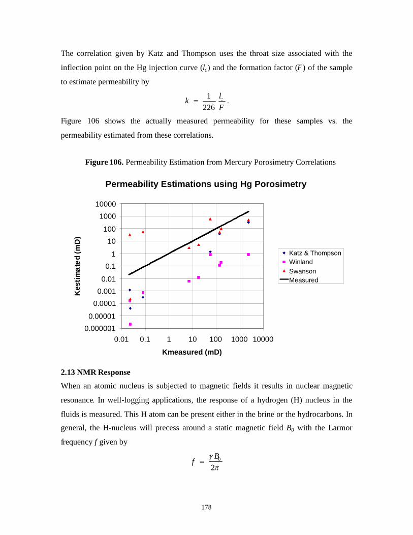
178
The correlation given by Katz and Thompson uses the throat size associated with the
inflection point on the Hg injection curve (lc) and the formation factor (F) of the sample
to estimate permeability by
1226
clkF
.
Figure 106 shows the actually measured permeability for these samples vs. the
permeability estimated from these correlations.
Figure 106. Permeability Estimation from Mercury Porosimetry Correlations
Permeability Estimations using Hg Porosimetry
0.000001
0.00001
0.0001
0.001
0.01
0.1
1
10
100
1000
10000
0.01 0.1 1 10 100 1000 10000
Kmeasured (mD)
Kes
tim
ate
d(m
D)
Katz & ThompsonWinlandSwansonMeasured
2.13 NMR Response
When an atomic nucleus is subjected to magnetic fields it results in nuclear magnetic
resonance. In well-logging applications, the response of a hydrogen (H) nucleus in the
fluids is measured. This H atom can be present either in the brine or the hydrocarbons. In
general, the H-nucleus will precess around a static magnetic field B0 with the Larmor
frequency f given by
0
2B
f

179
Whereγis the gyromagnetic ratio and for hydrogen
42.58 /2 MHz Tesla
From the theory of quantum mechanics, when a large number of protons are precessing
about a static magnetic field B0, with spins that can be parallel or anti-parallel to the
direction of B0, the net macroscopic magnetization of the system M0 is given by the
Curie’s law2 2
0 02
( 1)3(4 )h I I
M N BkT
where M0 = net magnetic moment per unit volume,
N = nuclei per unit volume,
k = Boltzman’s constant,
T = absolute temperature (K),
h = Plank’s constant,
I = spin quantum number of the nucleus.
When the field B0 is applied the magnetization is not instant but follows and exponential
growth
0 1( ) (1 exp( / ))zM t M t T
where T1 is the longitudinal relaxation time constant. When an oscillating field B1 with
frequency equal to the Larmor frequency is applied in a direction perpendicular to B0 the
macroscopic magnetization tips at an angle given by
1B
where τis the time over which B1 is applied. When diffusion can be ignored, the
irreversible decay of transverse magnetization can be measured using a CPMG pulse
sequence. The time constant of this decay is called the transverse relaxation time (T2) and
the equation is
0 2( ) exp( / )x xM t M t T
where M0x is the equilibrium transverse magnetization.
For fluids in pores, 3 types of relaxation contribute to the total decay in the signal
1. Bulk Relaxation,
2. Surface Relaxation, and
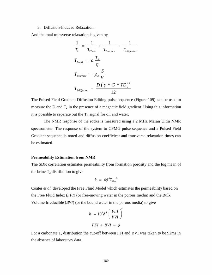
180
3. Diffusion-Induced Relaxation.
And the total transverse relaxation is given by
2 2 2 2
2
2 2
2
2
1 1 1 1
* *
12
bulk surface diffusion
Kbulk
surface
diffusion
T T T T
TT c
ST
V
D G TET
The Pulsed Field Gradient Diffusion Editing pulse sequence (Figure 109) can be used to
measure the D and T2 in the presence of a magnetic field gradient. Using this information
it is possible to separate out the T2 signal for oil and water.
The NMR response of the rocks is measured using a 2 MHz Maran Ultra NMR
spectrometer. The response of the system to CPMG pulse sequence and a Pulsed Field
Gradient sequence is noted and diffusion coefficient and transverse relaxation times can
be estimated.
Permeability Estimation from NMR
The SDR correlation estimates permeability from formation porosity and the log mean of
the brine T2 distribution to give4 2
24 lmk T
Coates et al. developed the Free Fluid Model which estimates the permeability based on
the Free Fluid Index (FFI) (or free-moving water in the porous media) and the Bulk
Volume Irreducible (BVI) (or the bound water in the porous media) to give2
4 410FFI
kBVI
FFI BVI
For a carbonate T2 distribution the cut-off between FFI and BVI was taken to be 92ms in
the absence of laboratory data.

181
Figure 107. Distinction between BVI and FFI using T2 cutoff
The model by Chang et al., takes the vugular cut-off of 750 ms and excludes the
contribution of vugs to the T2 log mean used for calculation of permeability. Their
correlation gives k from4 2
750 2 ,7504.75 lmk T
The permeability value estimated from these samples is plotted against the value
measured for the samples using single phase brine flood in Figure 108.
Figure 108. Permeability Estimation from NMR T2 Correlations
Permeability for NMR Correlation
0.0010.01
0.11
10100
100010000
0.01 1 100 10000
Kmeasured (mD)
kest
imat
ed(m
D)
Coates
Chang
SDR
Measured
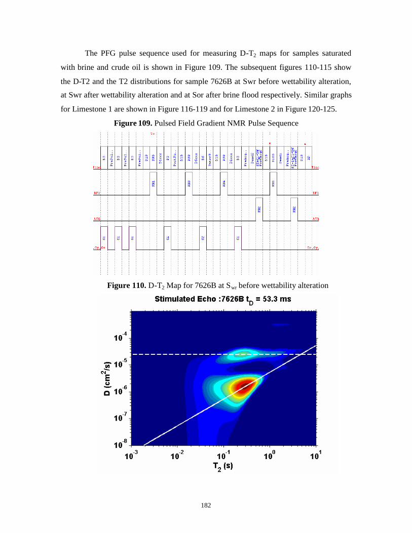
182
The PFG pulse sequence used for measuring D-T2 maps for samples saturated
with brine and crude oil is shown in Figure 109. The subsequent figures 110-115 show
the D-T2 and the T2 distributions for sample 7626B at Swr before wettability alteration,
at Swr after wettability alteration and at Sor after brine flood respectively. Similar graphs
for Limestone 1 are shown in Figure 116-119 and for Limestone 2 in Figure 120-125.
Figure 109. Pulsed Field Gradient NMR Pulse Sequence
Figure 110. D-T2 Map for 7626B at Swr before wettability alteration
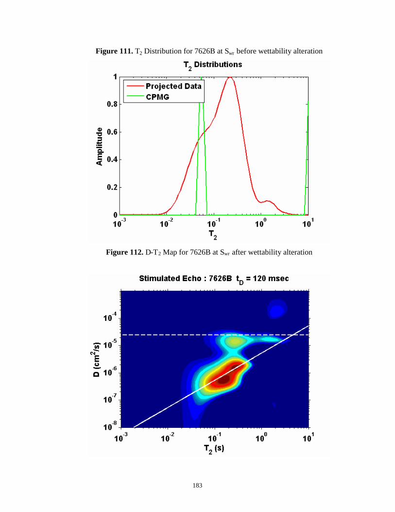
183
Figure 111. T2 Distribution for 7626B at Swr before wettability alteration
Figure 112. D-T2 Map for 7626B at Swr after wettability alteration

184
Figure 113. T2 Distribution for 7626B at Swr after wettability alteration
Figure 114. D-T2 Map for 7626B at Sor after brine flood
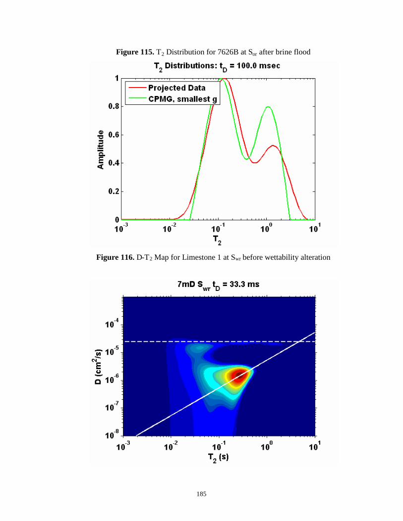
185
Figure 115. T2 Distribution for 7626B at Sor after brine flood
Figure 116. D-T2 Map for Limestone 1 at Swr before wettability alteration

186
Figure 117. T2 Distribution for Limestone 1 at Swr before wettability alteration
Figure 118. D-T2 Map for Limestone 1 at Swr after wettability alteration

187
Figure 119. T2 Distribution for Limestone 1 at Swr after wettability alteration
Figure 120. D-T2 map for Limestone 2 at Swr before wettability alteration

188
Figure 121. T2 Distribution for Limestone 2 at Swr before wettability alteration
Figure 122. D-T2 Map for Limestone 2 at Swr after wettability alteration
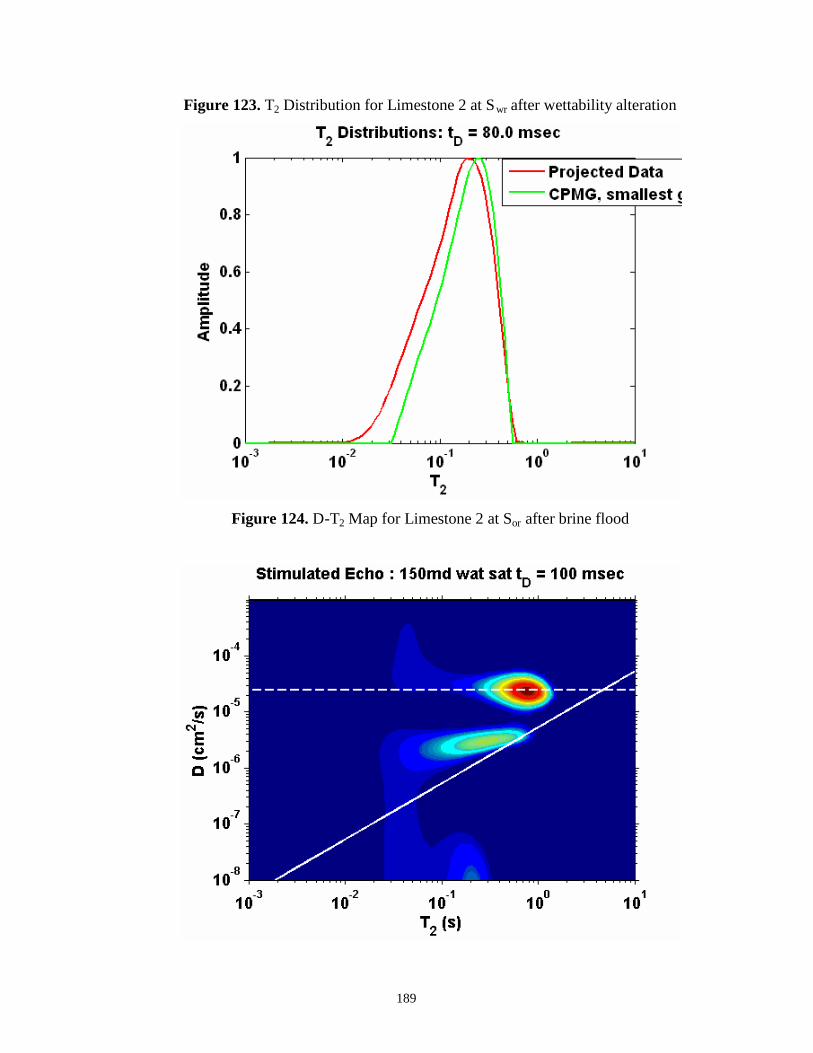
189
Figure 123. T2 Distribution for Limestone 2 at Swr after wettability alteration
Figure 124. D-T2 Map for Limestone 2 at Sor after brine flood

190
Figure 125. T2 Distribution for Limestone 2 at Sor after brine flood
The T2 distributions for brine saturated samples 2416, 7536B, 7626A and 7626B are
shown in Figures 125-129. These were measured using the CPMG pulse sequence.
Figure 126. T2 Distribution for Sample 2416 at 100% brine saturation
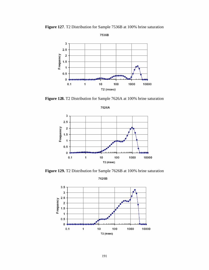
191
Figure 127. T2 Distribution for Sample 7536B at 100% brine saturation
Figure 128. T2 Distribution for Sample 7626A at 100% brine saturation
Figure 129. T2 Distribution for Sample 7626B at 100% brine saturation
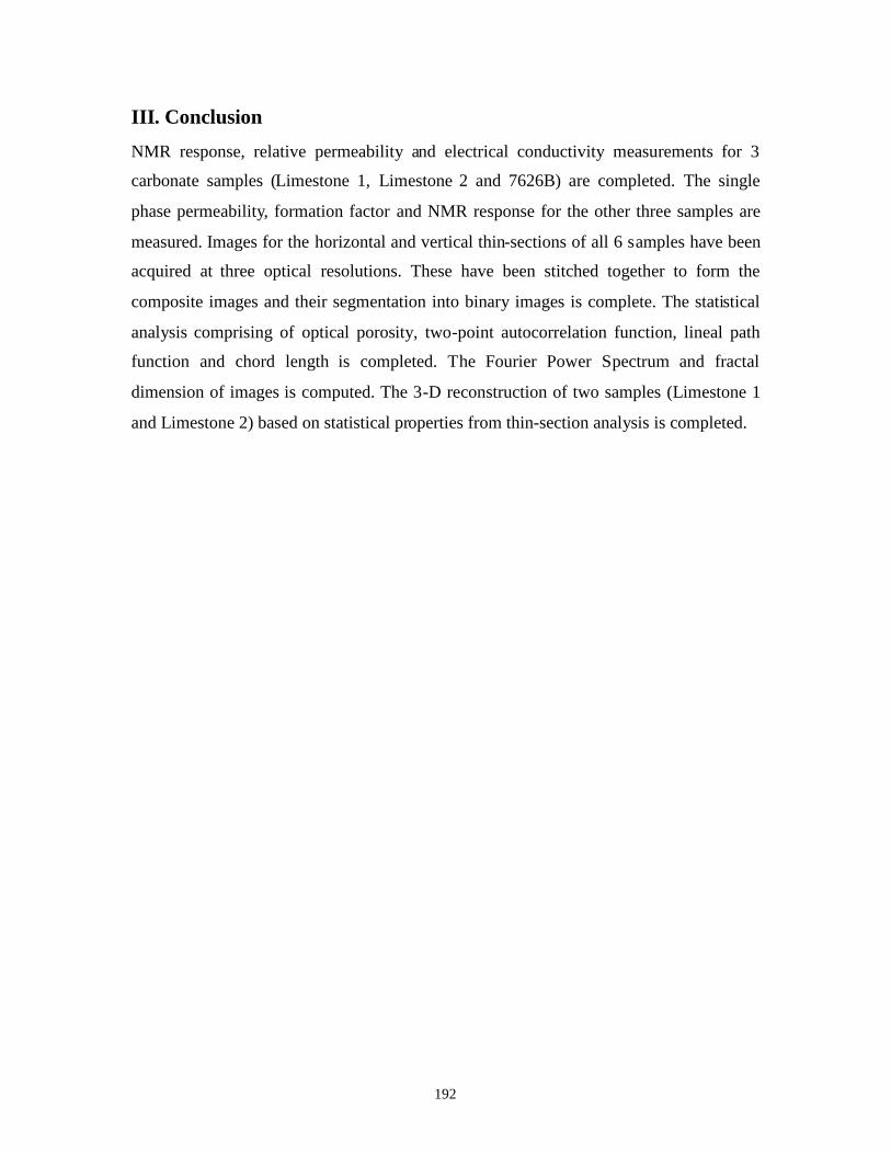
192
III. Conclusion
NMR response, relative permeability and electrical conductivity measurements for 3
carbonate samples (Limestone 1, Limestone 2 and 7626B) are completed. The single
phase permeability, formation factor and NMR response for the other three samples are
measured. Images for the horizontal and vertical thin-sections of all 6 samples have been
acquired at three optical resolutions. These have been stitched together to form the
composite images and their segmentation into binary images is complete. The statistical
analysis comprising of optical porosity, two-point autocorrelation function, lineal path
function and chord length is completed. The Fourier Power Spectrum and fractal
dimension of images is computed. The 3-D reconstruction of two samples (Limestone 1
and Limestone 2) based on statistical properties from thin-section analysis is completed.

193
DE-FC26-04NT15518
Integrated, Multi-Scale Characterization of Imbibition and WettabilityPhenomena Using Magnetic Resonance and Wide-Band DielectricMeasurements
NMR 1-D ProfilingMichael Rauschhuber and George Hirasaki
Abstract
T2 profiles can be generated by implementing the rapid acquisition withrelaxation enhancement (RARE) pulse sequence. The RARE sequence is amulti-echo imaging sequence used to construct a one-dimensional profile of T2relaxation times. Experimental parameters, such as sample size, gradientstrength and duration, and the number and spacing of the acquired data points,must be selected to ensure that useful information can be extracted from theprofiles. The sample must be centered within the Maran’s sweet spot. Thegradient strength relates the precession frequency to sample position.Attenuation due to diffusion is dependent on the product of gradient strength (g)and duration (). Therefore, g and should be selected in order to reduce theamount of the relaxation due to diffusion. The dwell time (DW), or spacingbetween acquired data points, needs to be selected so that the sample plus asmall region above and below is resolved by the experiment. The number ofdata points collected per echo will influence the image resolution; as more pointsare collected per echo, the resolution will increase. Experiments were performedon both a water sample and a layered water-squalane (C-30 oil, = 22 cP)system using the RARE sequence. T2 was calculated by fitting the decayingprofiles to a single exponential model. The difference between the T2 profilesacquired via RARE and the T2 of the bulk samples found using CPMG is due todiffusion and thus needs to be minimized.
While standard NMR techniques, such as CPMG or gradient CPMG, tendto look at either the whole sample or only a thin slice, NMR profiling relies on theapplication of imaging techniques in order to attain spatially resolvedmeasurements. Spatial resolution of properties such as magnetization andrelaxation times will allow for the determination of saturation profiles and sampleheterogeneities, such as changes in local porosity or pore size distribution. Thegoal of this project is to develop profiling techniques for a low-field NMR (2 MHzMaran Ultra) allowing for the determination of T2 as a function of sample position.

194
Outline of Report
Each section in this report addresses an essential topic for the generationof 1-D NMR profiles. First, the concept that spatially realization can be impartedonto a measurement via frequency encoding gradients will be addressed. Then,the basic spin echo imaging pulse sequence will be introduced as well as thenecessary parameter selection in order to generate a single 1-D image. The finaltopic covered will be the collection of multiple echoes using the rapid acquisitionwith relaxation enhancement (RARE) to produce a series of profiles from whichT2 can be extracted.
Frequency-Encoding Gradients
Frequency encoding is a standard MR technique used to detect spatialinformation from a desired sample. In a uniform magnetic field, protons precessat the same frequency, know as the Larmor frequency.
02Lf
(0.1)
When a magnetic gradient is applied, the intensity of the magnetic field andsubsequently, the precession frequency varies with spatial position. Forinstance, under the application of a linear gradient field, the spatially dependentprecession frequency can be represented by
0( )2 xf x B g x
(0.2)
or
( )2L xf x f g x
(0.3)
where gx designates the gradient strength and x denotes position. Therefore,spatial information can be extracted from the sample’s various precessionfrequencies. Consequently, gx is referred to as a frequency-encoding gradient(Bernstein et al., 2004).
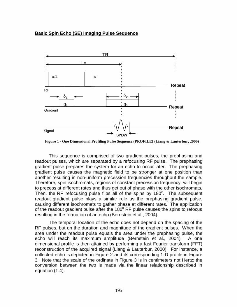
195
Basic Spin Echo (SE) Imaging Pulse Sequence
This sequence is comprised of two gradient pulses, the prephasing andreadout pulses, which are separated by a refocusing RF pulse. The prephasinggradient pulse prepares the system for an echo to occur later. The prephasinggradient pulse causes the magnetic field to be stronger at one position thananother resulting in non-uniform precession frequencies throughout the sample.Therefore, spin isochromats, regions of constant precession frequency, will beginto precess at different rates and thus get out of phase with the other isochromats.Then, the RF refocusing pulse flips all of the spins by 180o. The subsequentreadout gradient pulse plays a similar role as the prephasing gradient pulse,causing different isochromats to gather phase at different rates. The applicationof the readout gradient pulse after the 180o RF pulse causes the spins to refocusresulting in the formation of an echo (Bernstein et al., 2004).
The temporal location of the echo does not depend on the spacing of theRF pulses, but on the duration and magnitude of the gradient pulses. When thearea under the readout pulse equals the area under the prephasing pulse, theecho will reach its maximum amplitude (Bernstein et al., 2004). A onedimensional profile is then attained by performing a fast Fourier transform (FFT)reconstruction of the acquired signal (Liang & Lauterbur, 2000). For instance, acollected echo is depicted in Figure 2 and its corresponding 1-D profile in Figure3. Note that the scale of the ordinate in Figure 3 is in centimeters not Hertz; theconversion between the two is made via the linear relationship described inequation (1.4).
TE
Gradient
RF
Signal
TR
g1 g2
12
SI*DW
Repeat
Repeat
Repeat
TE
Gradient
RF
Signal
TR
g1 g2
12
SI*DW
Repeat
Repeat
Repeat
Figure 1 - One Dimensional Profiling Pulse Sequence (PROFILE) (Liang & Lauterbur, 2000)

196
2Larmor x Larmorf f g x x
(0.4)
where xLarmor corresponds to the sample height at which f = fLarmor.
6 6.5 7 7.5 8 8.5 9 9.5 10-1600
-1400
-1200
-1000
-800
-600
-400
-200
0
200
400
Sig
nala
mpl
itude
(a.u
.)
Time (msec)
Echo, g = 0.8 G cm-1, SI = 64, DW = 50sec
Figure 2 - Collected Echo for a Water Sample with a height of 4 cm.

197
0 500 1000 1500 2000 2500-3
-2
-1
0
1
2
3
Signal amplitude (a.u.)
h(c
m)
Water Profile, g = 0.8 G cm-1, SI = 64, DW = 50 sec
Figure 3 - Profile of 4 cm water sample generated after FFT reconstruction of the collectedecho.
Parameter Selection
NMR 1-D Profiles are sensitive to the selected measurement parameters.These include the sample size and location, the gradient strength (g) andduration (), and the number (SI) and spacing (DW) of the collected data points.
Sample Size and Location
The sample should be located within the sweet spot of the NMR andcentered about fLarmor. In order to determine the size and location of the sweetspot, a series of FID experiments where performed with water. The watersample has a height 0.5 cm and was moved in 0.5cm increments through theprobe; an FID was performed at each location. The results are illustrated inFigure 4. From these results, it was determined the sweet spot was about 5 cmlong. Therefore, for all subsequent measurements, the sample will be locatedwithin the sweet spot and have a height of 4 cm.

Gra
reliaHowTheovebehstre
Fi
FID Amplitude vs. Position
0
100
200
300
400
500
600
700
800
900
1000
0 1 2 3 4 5 6 7 8 9 10 11 12
Position (cm)
Am
pli
tud
ep
er
sca
n(a
.u.)
Figure 4 – Results of a series of FID experiments performed on a 0.5 cm sample of water used todetermine the sweet spot of the MARAN-M. The horizontal line denotes a 5% percent deviation
198
dient Strength
The gradient used for imaging should be the lowest value that will giveble results. Strong gradients can cause attenuation due to diffusion.ever, this effect can be minimized by selecting to use weaker gradients.refore, it is necessary to properly characterize the behavior of the gradientr a range of values. For instance, at very low gradients, the expectedavior deviates from what is observed. By using a low, reliable gradientngth, 0.800 G cm-1, attenuation due to diffusion can be reduced.
0.1
1
10
0.1 1 10
g predicted (G cm-1)
gob
ser
ved
(Gcm
-1)
gure 5 - Observed vs. Predicted behavior of the MARAN-M's gradient. Deviations are observedat very low values of g.
from the maximum amplitude.

199
Dwell Time
The dwell time (DW), or the spacing between the acquired data points,should be selected to acquire data over the length of the sample and a smalldistance beyond. If the dwell time is too short, the distance which themeasurement can identify is much longer than the length of the sample (Figure6).
0 2000 4000 6000 8000 10000 12000-15
-10
-5
0
5
10
15
Signal amplitude (a.u.)
h(c
m)
Water Profile, g = 0.8 G cm-1, SI = 64, DW = 10 sec
Figure 6 – Improper selection of DW. The measurement resolved a length much greaterthan the sample height.
The dwell time can be determined from the size of the sample and the strength ofthe gradient pulses used, and equation (1.6) gives a means of calculating anappropriate DW. This equation is based on the Nyquist sampling theorem whichstates that the sampling rate, SR, should be at least twice the maximumfrequency encoded in the signal where the maximum encoded frequency, fmax,corresponds to half the sample height plus a small distance outside for acentered sample (Bernstein et al., 2004). If this criterion is not meet, aliasing canoccur.
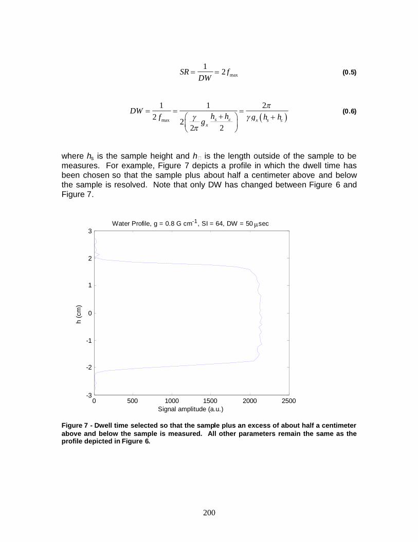
200
max
12SR f
DW (0.5)
max
1 1 22 2
2 2s x s
x
DWh hf g h hg
(0.6)
where hs is the sample height and h is the length outside of the sample to bemeasures. For example, Figure 7 depicts a profile in which the dwell time hasbeen chosen so that the sample plus about half a centimeter above and belowthe sample is resolved. Note that only DW has changed between Figure 6 andFigure 7.
0 500 1000 1500 2000 2500-3
-2
-1
0
1
2
3
Signal amplitude (a.u.)
h(c
m)
Water Profile, g = 0.8 G cm-1, SI = 64, DW = 50 sec
Figure 7 - Dwell time selected so that the sample plus an excess of about half a centimeterabove and below the sample is measured. All other parameters remain the same as theprofile depicted in Figure 6.

201
Number of Acquisition Points
The number of acquisition point (SI) is also a vital parameter whenperforming a profiling measurement. While DW determined the range offrequencies resolved, SI governs the number of points spanning that range.Therefore, increasing SI increases the image resolution.
s
points SIresolutioncm h h
(0.7)
2sh h
gDW
(0.8)
2
g DW SIpointsresolution
cm
(0.9)
However, acquisition must occur under a gradient and is therefore limitedby the readout gradient duration (2). Therefore, the duration of the gradientpulse must be greater than or equaled to the product of SI and DW (Eq. 1.10).Increasing the gradient duration to accommodate more points will increaseresolution at the cost of greater attenuation due to diffusion.
2 SI DW (0.10)
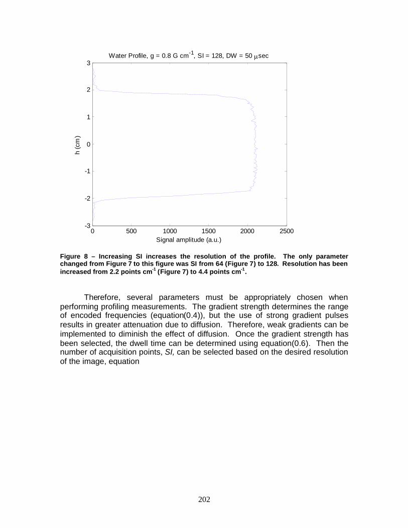
202
0 500 1000 1500 2000 2500-3
-2
-1
0
1
2
3
Signal amplitude (a.u.)
h(c
m)
Water Profile, g = 0.8 G cm-1, SI = 128, DW = 50 sec
Figure 8 – Increasing SI increases the resolution of the profile. The only parameterchanged from Figure 7 to this figure was SI from 64 (Figure 7) to 128. Resolution has beenincreased from 2.2 points cm-1 (Figure 7) to 4.4 points cm-1.
Therefore, several parameters must be appropriately chosen whenperforming profiling measurements. The gradient strength determines the rangeof encoded frequencies (equation(0.4)), but the use of strong gradient pulsesresults in greater attenuation due to diffusion. Therefore, weak gradients can beimplemented to diminish the effect of diffusion. Once the gradient strength hasbeen selected, the dwell time can be determined using equation(0.6). Then thenumber of acquisition points, SI, can be selected based on the desired resolutionof the image, equation
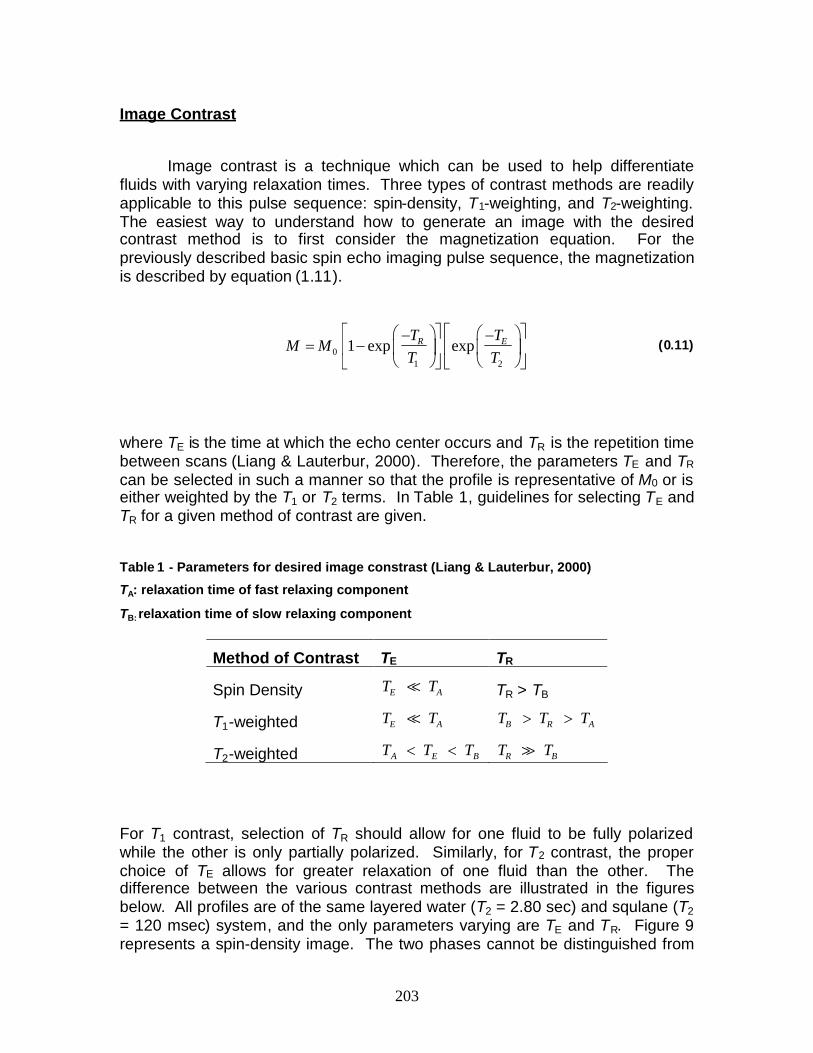
203
Image Contrast
Image contrast is a technique which can be used to help differentiatefluids with varying relaxation times. Three types of contrast methods are readilyapplicable to this pulse sequence: spin-density, T1-weighting, and T2-weighting.The easiest way to understand how to generate an image with the desiredcontrast method is to first consider the magnetization equation. For thepreviously described basic spin echo imaging pulse sequence, the magnetizationis described by equation (1.11).
01 2
1 exp expR ET TM M
T T
(0.11)
where TE is the time at which the echo center occurs and TR is the repetition timebetween scans (Liang & Lauterbur, 2000). Therefore, the parameters TE and TR
can be selected in such a manner so that the profile is representative of M0 or iseither weighted by the T1 or T2 terms. In Table 1, guidelines for selecting TE andTR for a given method of contrast are given.
Table 1 - Parameters for desired image constrast (Liang & Lauterbur, 2000)
TA: relaxation time of fast relaxing component
TB: relaxation time of slow relaxing component
Method of Contrast TE TR
Spin Density E AT T TR > TB
T1-weighted E AT T B R AT T T
T2-weighted A E BT T T R BT T
For T1 contrast, selection of TR should allow for one fluid to be fully polarizedwhile the other is only partially polarized. Similarly, for T2 contrast, the properchoice of TE allows for greater relaxation of one fluid than the other. Thedifference between the various contrast methods are illustrated in the figuresbelow. All profiles are of the same layered water (T2 = 2.80 sec) and squlane (T2= 120 msec) system, and the only parameters varying are TE and TR. Figure 9represents a spin-density image. The two phases cannot be distinguished from

204
one another because both water and squalane have similar hydrogen indexes.On the other hand, the squalane layer in a T1-weighted image (Figure 10) has amuch larger amplitude because it is allowed to fully polarize between scans whilethe water is not. Finally, Figure 11 is an illustration of a T2-weighted image inwhich both phases are allowed to fully polarize between scans. Therefore, along TE results in greater relaxation in the oil phase and, subsequently, greateramplitude of the water phase. However, the longer TE will also result inrelaxation due to diffusion if the gradient is too large.
0 500 1000 1500 2000 2500-3
-2
-1
0
1
2
3
Signal amplitude (a.u.)
h(c
m)
Spin Density Image of a Layered Water-Squalane Sample (TE = 8 msec, TR = 15,000 msec)
Figure 9 – Spin Density image of a layered water and squalane system

205
0 500 1000 1500 2000 2500-3
-2
-1
0
1
2
3
Signal amplitude (a.u.)
h(c
m)
T1-Weighted Image of a Layered Water-Squalane Sample (TE = 8 msec, TR = 714 msec)
Figure 10 – T1-weighted image of a layered water and squalane system
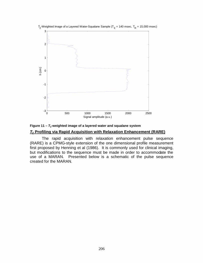
206
0 500 1000 1500 2000 2500-3
-2
-1
0
1
2
3
Signal amplitude (a.u.)
h(c
m)
T2-Weighted Image of a Layered Water-Squalane Sample (TE = 140 msec, TR = 15,000 msec)
Figure 11 – T2-weighted image of a layered water and squalane system
T2 Profiling via Rapid Acquisition with Relaxation Enhancement (RARE)
The rapid acquisition with relaxation enhancement pulse sequence(RARE) is a CPMG-style extension of the one dimensional profile measurementfirst proposed by Henning et al (1986). It is commonly used for clinical imaging,but modifications to the sequence must be made in order to accommodate theuse of a MARAN. Presented below is a schematic of the pulse sequencecreated for the MARAN.

…
RF
Gradient
Signal
…
…g1 g2 g2
1
12 2
…
RF
Gradient
Signal
…
…g1 g2 g2
1
12 2
207
In the above schematic, the first gradient pulse is known as the pre-phasing pulse and all subsequent gradient pulses are referred to as readout orimaging pulses. Both pulses play analogous roles as their counterparts in theone dimensional profiling pulse sequence with one significant exception. As inthe profiling sequence, the temporal location of the echo occurs when the area ofthe readout pulse is equivalent to the area under the prephasing pulse.Therefore, the remainder of the readout pulse acts as a prephasing pulse for thenext echo. Resulting from this fact stems a careful balance between the twogradient pulses. In other words, the readout pulse should have twice the area ofthe prephasing pulse. In Figure 12, note that 2g11 = g22.
The Fourier transform can be taken for each individual echo to obtain aseries of one-dimensional profiles. The attenuation in the signal is alsoobservable in the profiles. Therefore, the goal behind using such a sequence isto take advantage of the frequency encoding gradients and extract T2 informationas a function of position within the sample. A series of profiles with an increasingamount of T2 relaxation generated by the RARE sequence is shown in Figure 13.
Figure 12 - RARE Pulse Sequence Diagram (Bernstein et al., 2004)

208
0 200 400 600 800 1000 1200 1400 1600 1800-4
-3
-2
-1
0
1
2
3
4Water Profiles via RARE
Signal amplitude (a.u.)
h(c
m)
echo #1echo #2echo #4echo #8echo #16echo #32echo #64echo #128echo #256echo #512echo #1024
Figure 13 – RARE Profiles of a water sample with a 4 cm height. g1 = g2 = 0.800 cm-1,
1 = 1.30 msec, = 3.00 msec, DW = 40.0 msec, SI = 64
Effect of Diffusion
Due to the presence of multiple gradient pulses, attenuation due todiffusion can become significant. Therefore, it is necessary to develop a suitablemodel describing the attenuation in terms of the relevant parameters of the pulsesequence. Callaghan (1991) suggests that one method which can be used todetermine the effect of self-diffusion is the application of the Bloch-Torreyequations. In the rotating reference frame, the effect of self-diffusion and velocityon the transverse magnetization, MT, can be represented by (Torrey, 1956)
2
2
-T TT T T
M Mi M D M M
t T
r g v (0.12)
With the solution (Stejskal and Tanner, 1965)

209
20
( , ) ( ) exp ( ') ' expt
T
tM t A t i t dt
T
r r g (0.13)
At the echo center,0
( ') 't
t dtg is equaled to zero. Therefore, equation (0.13)
reduces to
2( , ) ( ) expT
tM t A t T
r (0.14)
Substituting equation (0.14) into equation (0.12) yields an expression for A(t).
2
20
( )( ') ' exp
tA t tD t dt
t T
g (0.15)
2' '2
0 0 0 0
( ) exp ( '') '' ' exp ( '') '' 't t t t
A t D t dt dt i t dt dt
g v g (0.16)
If there is no flow, this expression can be reduced to
2'2
0 0
( ) exp ( '') '' 't t
A t D t dt dt
g (0.17)
This formulation neglects the presence of RF pulses. However, the effect of theRF pulses can be accounted for by examining the “effective gradient”. When a pulse is applied, the phase shift due to the presence of the gradient is flipped.This is equivalent to applying a gradient pulse with the opposite polarity.Therefore, the effective gradient, g*, can be thought of as gradient pulsesrequired to refocus the signal in the absence of 180 RF pulses, and isrepresented in the following figure for the RARE sequence.

EfEf
210
Or the effective gradient, g*(t), can be defined as
0 when 0< t <d
-g1 when d< t <d+1
0 when d+1 < t < d + 1
g2 when d + 1 < t < 2+ 2/2
0 when 2+ 2/2 < t < 4- 2/2
-g2 when 4- 2/2< t < 4+ 2/2
0 when 4+ 2/2 < t < 6- 2/2
g2 when 6- 2/2< t < 6+ 2/2
…
-g2 when 2n- 2/2< t < 2n+ 2/2, where n, the number of echoes iseven.
Using these facts and imposing the stipulation that g1 = g2 = g and 21 =2, A(t) takes the form
RF
Gradient
…
…
…
g1 g2 g2
1
1
2 2
fective Gradient
g1
g2
g2
2
2
d
1
RF
Gradient
…
…
…
g1 g2 g2
1
1
2 2
fective Gradient
g1
g2
g2
2
2
d
1
Figure 14 – Representation of the effective gradient, g* , in the RARE sequence.

211
2 2 21 1 2
( 1)( ) exp 2( 1)3
nA t D g n (0.18)
Therefore, the magnetization at the echo center of the RARE sequence can bedescribed by
2 2 21 1 2
0 2
( 1)exp 2( 1) exp3
M n tD g nM T
(0.19)
Where n is the number of echoes. A comparison of this equation to experimentalresults can be seen in Figure 15 and Figure 16. Water was used as the sample.The blue curve represents the CPMG decay, the green curve is the decay of theRARE profiles at the specified sample location, and the red curve is thecalculated behavior.
0 1000 2000 3000 4000 5000 600010-1
100
RARE Attenuation of Water, g1 = g2 = 0.800 G cm-1, h = 0 cm
Time (msec.)
Nor
mal
ized
Sig
nalA
mpl
itude
(a.u
.)
CPMGRARECalculated RARE
Figure 15 Comparison of CPMG with RARE for g = 0.8 G/cm
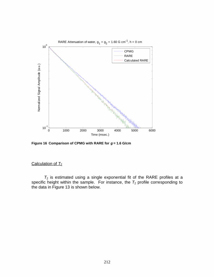
212
0 1000 2000 3000 4000 5000 600010
-1
100
RARE Attenuation of water, g1 = g2 = 1.60 G cm-1, h = 0 cm
Time (msec.)
Nor
mal
ized
Sig
nalA
mpl
itude
(a.u
.)
CPMGRARECalculated RARE
Figure 16 Comparison of CPMG with RARE for g = 1.6 G/cm
Calculation of T2
T2 is estimated using a single exponential fit of the RARE profiles at aspecific height within the sample. For instance, the T2 profile corresponding tothe data in Figure 13 is shown below.
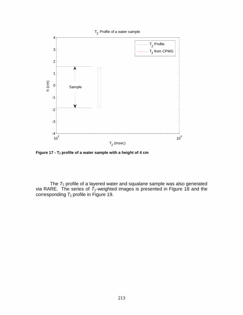
213
103
104
-4
-3
-2
-1
0
1
2
3
4
T2 (msec)
h(c
m)
T2 Profile of a water sample
T2
Profile
T2 from CPMG
Sample
Figure 17 - T2 profile of a water sample with a height of 4 cm
The T2 profile of a layered water and squalane sample was also generatedvia RARE. The series of T2-weighted images is presented in Figure 18 and thecorresponding T2 profile in Figure 19.

214
0 200 400 600 800 1000 1200 1400 1600 1800-4
-3
-2
-1
0
1
2
3
4Profiles of a layered water-squalane sample via RARE
Signal amplitude (a.u.)
h(c
m)
echo #1echo #2
echo #4echo #8echo #16echo #32echo #64echo #128
echo #256echo #512echo #1024
Figure 18 - RARE Profiles of a layered water and squalane sample. Each layer has a heightof 2 cm. g1 = g2 = 0.824 G cm-1, 1 = 1.30 msec, = 3.00 msec, DW = 39.0 msec, SI = 64

215
101
102
103
104
-4
-3
-2
-1
0
1
2
3
4
T2 (msec)
h(c
m)
T2 Profile of a layered water-squalane sample
Sample
Figure 19 - T2 profile of layered water and squalane system. Each layer has a height of 2cm.
Conclusion
In summary, NMR profiling is a valuable tool enabling for thedetermination of spatial characteristics of a sample. When parameters areproperly selected, useful information can be extracted from NMR profiles. Theseparameters include the gradient strength, dwell time, and the number ofacquisition points. The gradient imparts spatial realization upon themeasurements, but can also cause attenuation due to diffusion. Therefore, gand should be chosen to reduce the effect of relaxation due to diffusion. Also,DW and SI affect the resolution of the 1-D profiles. DW should narrow the rangeof the measurement to a span which is a little greater than the sample length,and SI will determine the number points over the range set by DW.
Furthermore, by taking advantage of differing relaxation times within asample, images with different types of contrast, such as spin-density, T1-weighted, and T2-weighted, can be generated. By comparing several imageswhich have undergone various amounts of relaxation, T2 can be calculated as afunction of time. The rapid acquisition with relaxation enhancement (RARE)pulse sequence can be used to generate multiple profiles each with a differentamount of T2-weighting. Experiments have been performed with both a watersample and a layered water-squalane system. The results are in goodagreement with the expected behavior for the RARE sequence and indicate thatthis is an effective method for obtaining T2 profiles.

216
References
Bernstein, M.A., King, K.F., & Zhou, X.J. (2004). Handbook of MRI pulsesequences. Amsterdam: Elsevier Academic Press.
Callaghan, P.T. (1991) Principles of nuclear magnetic resonance microscopy.New York: Oxford University Press, Inc.
Henning, J., Nauerth, A., & Friedburg, H. (1986). RARE imaging: A fast imagingmethod for clinical MR. Magnetic Resonance in Medicine, 3, 823-833.
Liang, Z.P., & Lauterbur, P.C (2000). Principles of magnetic resonance imaging:A, signal processing perspective. New York, NY: IEEE Press.
Stejskal, E.O., & Tanner,J.E. (1965). Spin diffusion measurements: Spin-echoesin the presence of a time-dependent field gradient. The Journal of ChemicalPhysics, 42(1), 288-292.
Torrey, H.C. (1956). Bloch equations with diffusion terms. Physical Review,104(3), 563-565