Flux tubes in U(1) Lattice Gauge Theory

Andre da Conceicao Amado

Dissertacao para a obtencao de Grau de Mestre em

Engenharia Fısica Tecnologica

Juri

Presidente: Prof. Maria Teresa Haderer de la Pena Stadler

Orientador: Prof. Pedro Jose de Almeida Bicudo

Vogal: Prof. Pedro Domingos Santos do Sacramento

Vogal: Doutor Paulo de Jesus Henriques da Silva

Outubro 2012

Acknowledgements

I would like to thank my supervisor Prof. Pedro Bicudo for all the help, support and important advices

provided, and for the patience, attending to my requests even when sometimes made close to the deadline.

Also I want to thank Nuno Cardoso and Marco Cardoso for helping me in several situations, either with

computational or Lattice QCD problems.

I thank Marina Marinkovic as the first person teaching me formally about Lattice QCD in a seminar that

had a deep impact on my way of regarding Lattice QCD when I was starting to study the subject.

Also I wish to extend my warmest regards to present and past The Office population, resident or sporadic,

with whom I shared much more than a working place. All kinds of discussions either about physics, languages

or politics, as well as the coffee breaks and nonsense ideas, so important to keep mental sanity and which

make that place such a good place to work. I want to thank in particular Miguel Romao, Nuno Ribeiro,

Pedro Loreto, Miguel Fernandes, Angeles Moline, Carolina Arbelaez, David Vanegas, Maria Joao Carrilho,

Antonio Pacheco, Leonardo Pedro, Pedro Polvora...

I am thankful to CFTP and IST for the good working conditions provided. This work was partly funded

by the FCT contracts CERN/FP/116383/2010 and CERN/FP/123612/2011, and by a NVIDIA Academic

Partnership and NVIDIA Teaching Grant.

Last but not least a special thank to Azadeh Mohammadi for the discussions, joyful laughing and so much

more. Kheili mamnunam Azadeh jun.

I thank all these people, as well as my family and many other friends, for the friendship and continued

support provided which were essential to this work and throughout my life.

iii

Resumo

Neste trabalho implementamos um codigo numerico com vista a estudar varios aspectos de Teoria de Gauge

na Rede U(1), principalmente propriedades da fase confinante.

Comecamos com uma introducao geral ao tema de Teoria de Gauge na Rede.

Utilizamos correlacoes de loops de Polyakov para estudar tubos de fluxo em U(1) compacto a 4D e o

potencial estatico electrao positrao em teoria de gauge na rede. Utilizando operadores de campo medimos

directamente os campos electrico e magnetico. Estudamos ainda a evolucao do potencial com β, assim como

outras quantidades ja bem conhecidas. De modo a melhorar a razao sinal-ruıdo na fase confinante, aplicamos

o algoritmo multinıvel de Luscher e Weiss.

Estudamos um intervalo de temperaturas de 0.05 Tc a 0.40 Tc e os nossos resultados seguem as previsoes

da Teoria de Cordas Efectiva em todo o intervalo. Conseguimos observar a transicao do comportamento

logarıtmico para o linear.

O nosso codigo esta completamente escrito em CUDA, e corremo-lo em unidades de processamento grafico

de geracao FERMI da NVIDIA, de modo a atingir o desempenho necessario aos nossos calculos.

Palavras-chave: Teoria de Gauge na Rede, U(1), tubos de fluxo, Cromodinamica Quantica na Rede,

potencial estatico, Teoria de Cordas Efectiva

v

Abstract

In this work we implement a numerical code to study several aspects of U(1) Lattice Gauge Theory, mainly

properties of confining phase.

We start with a general introduction to the subject of Lattice Gauge Theory.

We utilize Polyakov loop correlations to study 4D compact U(1) flux tubes and the static electron-

positron potential in lattice gauge theory. By using field operators we are able to probe directly the electric

and magnetic fields. Also we study the evolution of the potential with β as well as other already well-known

quantities. In order to improve the signal-to-noise ratio in the confinement phase, we apply the Luscher-Weiss

multilevel algorithm.

We study a range of temperatures from 0.05 Tc to 0.40 Tc and our results follow the Effective String

Theory prediction for the relation between the the static charge distance and the width of the tube flux in

the whole range. We are able to observe the transition from logarithmic to linear behavior.

Our code is completely written in CUDA, and we run it in NVIDIA FERMI generation GPU’s, in order

to achieve the necessary performance for our computations.

Keywords: Lattice Gauge Theory, U(1), flux tubes, Lattice QCD, static potential, Effective String

Theory

vii

Contents

Acknowledgements . . . . . . . . . . . . . . . . . . . . . . . . . . . . . . . . . . . . . . . . . . . . . iii

Resumo . . . . . . . . . . . . . . . . . . . . . . . . . . . . . . . . . . . . . . . . . . . . . . . . . . . v

Abstract . . . . . . . . . . . . . . . . . . . . . . . . . . . . . . . . . . . . . . . . . . . . . . . . . . . vii

Contents ix

List of Tables xi

List of Figures xiii

1 Introduction and Motivation 1

1.1 Lattice Quantum Field Theory . . . . . . . . . . . . . . . . . . . . . . . . . . . . . . . . . . . 2

1.2 Temperature . . . . . . . . . . . . . . . . . . . . . . . . . . . . . . . . . . . . . . . . . . . . . 9

1.3 Effective String Theory . . . . . . . . . . . . . . . . . . . . . . . . . . . . . . . . . . . . . . . 9

2 Methods 11

2.1 Generation of configurations . . . . . . . . . . . . . . . . . . . . . . . . . . . . . . . . . . . . . 11

2.2 Multihit . . . . . . . . . . . . . . . . . . . . . . . . . . . . . . . . . . . . . . . . . . . . . . . . 14

2.3 Luscher-Weisz Multilevel . . . . . . . . . . . . . . . . . . . . . . . . . . . . . . . . . . . . . . . 15

2.4 Sommer scale . . . . . . . . . . . . . . . . . . . . . . . . . . . . . . . . . . . . . . . . . . . . . 19

2.5 CUDA . . . . . . . . . . . . . . . . . . . . . . . . . . . . . . . . . . . . . . . . . . . . . . . . . 20

2.6 Other computational resources . . . . . . . . . . . . . . . . . . . . . . . . . . . . . . . . . . . 22

3 Results 23

3.1 Average plaquette density . . . . . . . . . . . . . . . . . . . . . . . . . . . . . . . . . . . . . . 23

3.2 Confining phase transition . . . . . . . . . . . . . . . . . . . . . . . . . . . . . . . . . . . . . . 23

3.3 Sommer scale . . . . . . . . . . . . . . . . . . . . . . . . . . . . . . . . . . . . . . . . . . . . . 25

3.4 Multilevel convergence . . . . . . . . . . . . . . . . . . . . . . . . . . . . . . . . . . . . . . . . 26

3.5 Potential . . . . . . . . . . . . . . . . . . . . . . . . . . . . . . . . . . . . . . . . . . . . . . . . 26

3.6 Flux tube profile . . . . . . . . . . . . . . . . . . . . . . . . . . . . . . . . . . . . . . . . . . . 30

3.7 Flux tube width . . . . . . . . . . . . . . . . . . . . . . . . . . . . . . . . . . . . . . . . . . . 32

3.8 Field in finite temperature . . . . . . . . . . . . . . . . . . . . . . . . . . . . . . . . . . . . . . 34

3.9 Field in non-confining phase . . . . . . . . . . . . . . . . . . . . . . . . . . . . . . . . . . . . . 34

4 Conclusion 41

A Notation and Definitions 43

ix

Bibliography 45

x

List of Tables

2.1 Specifications of the GPU’s used in this work. . . . . . . . . . . . . . . . . . . . . . . . . . . . . . 21

3.1 Dependence of r0/a and temperature with Nt. . . . . . . . . . . . . . . . . . . . . . . . . . . . . 26

3.2 Fit parameters of potential of two static charges at different β. The fit function is V (r) = A+b/r+σr. 28

3.3 σ in function of Nt for β = 1.00. . . . . . . . . . . . . . . . . . . . . . . . . . . . . . . . . . . . . 30

3.4 Widths and fit parameters of the width expression. . . . . . . . . . . . . . . . . . . . . . . . . . . 32

xi

List of Figures

1.1 Evolution of αS with the scale as function of energy scale (figure from [1]). . . . . . . . . . . . . 2

1.2 Fermions and gauge fields. . . . . . . . . . . . . . . . . . . . . . . . . . . . . . . . . . . . . . . . . 3

1.3 Plaquette. . . . . . . . . . . . . . . . . . . . . . . . . . . . . . . . . . . . . . . . . . . . . . . . . . 4

2.1 Reflection of the phase in overrelaxation method, conserving the action constant. . . . . . . . . . 13

2.2 Correlation of configurations in function of number of updates, with and without the use of

overrelaxation method, for a lattice with β = 4 and volume 244. . . . . . . . . . . . . . . . . . . . 13

2.3 Correlation of configurations in function of number of updates, for different amount of overrelax-

ation steps, for a lattice with β = 4 and volume 244. . . . . . . . . . . . . . . . . . . . . . . . . . 14

2.4 Two-link operator, as part of a Polyakov loop. . . . . . . . . . . . . . . . . . . . . . . . . . . . . 16

2.5 Multilevel method for Polyakov loop correlations. . . . . . . . . . . . . . . . . . . . . . . . . . . . 17

2.6 Multilevel method for electromagnetic field. . . . . . . . . . . . . . . . . . . . . . . . . . . . . . . 19

2.7 CUDA memory architecture. . . . . . . . . . . . . . . . . . . . . . . . . . . . . . . . . . . . . . . 22

3.1 Plaquette susceptibility with β in a 4D 84 lattice. . . . . . . . . . . . . . . . . . . . . . . . . . . . 23

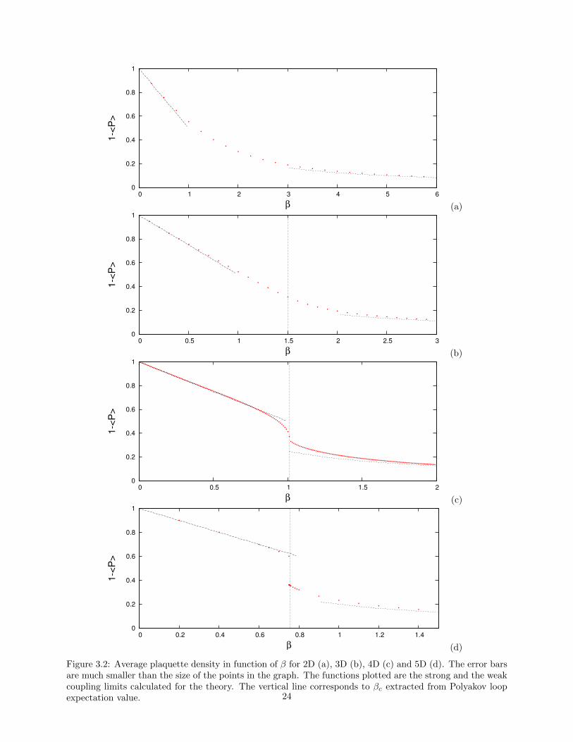
3.2 Average plaquette density in function of β for 2D (a), 3D (b), 4D (c) and 5D (d). The error

bars are much smaller than the size of the points in the graph. The functions plotted are the

strong and the weak coupling limits calculated for the theory. The vertical line corresponds to βc

extracted from Polyakov loop expectation value. . . . . . . . . . . . . . . . . . . . . . . . . . . . 24

3.3 Polyakov loop expectation value with β in a 4D 84 lattice (the error bars are smaller than the size

of the points). . . . . . . . . . . . . . . . . . . . . . . . . . . . . . . . . . . . . . . . . . . . . . . . 25

3.4 Plaquette susceptibility in function of β in a lattice 243 × 4. . . . . . . . . . . . . . . . . . . . . . 25

3.5 Polyakov loop correlation convergence with multilevel iterate. . . . . . . . . . . . . . . . . . . . . 26

3.6 Potential of two static charges at β = 1. The error bars are much smaller than the size of the

points in the graph. . . . . . . . . . . . . . . . . . . . . . . . . . . . . . . . . . . . . . . . . . . . 27

3.7 Potential of two static charges at β = 3. The error bars are much smaller than the size of the

points in the graph. . . . . . . . . . . . . . . . . . . . . . . . . . . . . . . . . . . . . . . . . . . . 28

3.8 Dependence of string tension with β in 4D. . . . . . . . . . . . . . . . . . . . . . . . . . . . . . . 29

3.9 Dependence of 1/r term with β in 4D (normalized to π/12). . . . . . . . . . . . . . . . . . . . . . 29

3.10 σ extracted from potential fit at β = 1.00 for different Nt values. The curve is the theoretical

expectation from Effective String Theory at 2-loops (χ2 = 0.006). Notice that the expression is

not fitted, since the only parameter (σ0) is fixed by zero temperature result. . . . . . . . . . . . . 30

3.11 Flux tube profile for several charge distances at β = 1.00 and Nt = 24 (T = 0.053Tc). . . . . . . 31

3.12 Flux tube profile for several charge distances at β = 1.00 and Nt = 4 (T = 0.40Tc). . . . . . . . . 31

xiii

3.13 Squared width in function of charge separation for 24 (a), 12 (b), 8 (c) and 4 (d). The figures on

the left are plots of a2w2(r/a) vs log(r/a) and on the right a2w2(r/a) vs r/a. . . . . . . . . . . . 33

3.14 Electric field in charges’ plan for charge separations of 2, 4, 6 and 8 lattices units in a 243 × 4 4D

lattice at β = 1. . . . . . . . . . . . . . . . . . . . . . . . . . . . . . . . . . . . . . . . . . . . . . . 34

3.15 Electric field in charges’ plan for charge separations of 2, 4, 6 and 8 lattices units in a 244 4D

lattice at β = 3. . . . . . . . . . . . . . . . . . . . . . . . . . . . . . . . . . . . . . . . . . . . . . . 35

3.16 Absolute value of electric field in charges’ plan for charge separations of 2, 4, 6 and 8 lattices units

in a 243 × 8 4D lattice at β = 1. . . . . . . . . . . . . . . . . . . . . . . . . . . . . . . . . . . . . 36

3.17 Field line plot of electric field in charges’ plan for charge separations of 2, 4, 6 and 8 lattices

units in a 243 × 4 4D lattice at β = 1. The colors correspond to a threshold to make it easier to

visually separate the stronger field caused by the charges from the small random fluctuations of

the background (where red corresponds to the stronger field). . . . . . . . . . . . . . . . . . . . . 37

3.18 Absolute value of electric field in charges’ plan for charge separations of 2, 4, 6 and 8 lattices units

in a 243 × 8 4D lattice at β = 3. . . . . . . . . . . . . . . . . . . . . . . . . . . . . . . . . . . . . 38

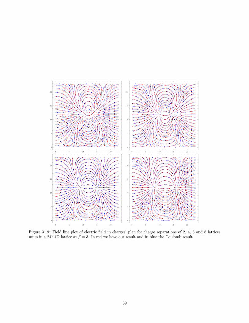
3.19 Field line plot of electric field in charges’ plan for charge separations of 2, 4, 6 and 8 lattices units

in a 244 4D lattice at β = 3. In red we have our result and in blue the Coulomb result. . . . . . . 39

xiv

Chapter 1

Introduction and Motivation

Lattice Quantum Field Theory is an area of study increasingly important in Quantum Field Theory. The

recent important advances, both theoretical and of computational capacity, open new horizons of study and

allow this theory to reach areas it could not before.

Lattice Quantum Field Theory opens the possibility of a better understanding of confining mechanisms

an area of study closed to the usage of perturbative tools.

In the context of this formalism we can study of the details of the interactions in order to compare then

with other theoretical models, like Effective String Theory, and get a better understanding of the virtues

and limitations of this kind of effective models. It is important to check these predictions in the context of

different groups. This result is already well set in 3D for SU(2) gauge group and some other groups (like

Z2) and some studies are being conducted in this moment like with SU(3) gauge group. Some studies have

been done in U(1) gauge group although its results are not yet completely well established. We decided to

study the structure of flux tubes produced by static charges in U(1) lattice gauge theory in order to try to

give a contribution to settle this subject.

Although sometimes the introductory parts are written in a more general frameset, the objective of this

dissertation is to study U(1) lattice gauge theory. It assumes knowledge of basic quantum field theory by the

reader.

We decided to write our code completely in CUDA because, although we have the drawback of being

significantly more difficult to program, we can achieve much better performances due to the possibility of

writing a highly parallelized code. CUDA requires knowledge about the architecture of the GPU to be used

and careful planning of the memory usage to achieve better results.

We advise the reader non familiarized with the notation to take a glance at appendix A on notation and

definitions frequently used throughout this text and maybe use it as reference.

In this chapter we introduce some steps on building a Lattice Quantum Field Theory as well as a small

introduction of the relevant results of Effective Field Theory in the context of this work. In the second

chapter we introduce the numerical methods used in our calculations and present the results in third chapter.

Finally a conclusion where we make a summary of our results and present some paths that, in our opinion,

can be worth exploring in the sequence of this work.

1

1.1 Lattice Quantum Field Theory

Lattice Quantum Field Theory is a discretized Quantum Field Theory that allows to perform non-perturbative

numerical Quantum Field Theory computations, as well as some analytical calculations, including perturba-

tive ones.

Lattice Gauge Theory (LGT) was first proposed by Wilson in 1974 [2] as an alternative ultraviolet cutoff

method, allowing to perform analytical computations and obtaining continuum limits.

Soon after people started to explore the possibilities that lattice approach opens in direct numerical eval-

uation of gauge theories. In 1981 Hamber and Parisi publish for the first time a hadronic mass spectrum

obtained from lattice QCD in quenched approximation [3], demonstrating in practice the possibility of per-

forming this kind of calculations. With time Lattice Gauge Theory became regarded as the natural way for

calculating numerical non-perturbative quantities.

Progressively people obtained a much deeper understanding of systematical errors and the 2000’s, with the

development of algorithms and computational power, have seen the appearance of unquenched calculations,

with the effects of quark loops being taken into account.

Although in 2001 people feared it would be impossible to reach realistic quark masses, independently

of computational power available, due to an enormous rise in the calculation time needed with the algo-

rithms available, the recent development of new algorithms solved this problem and opened the possibility

of approaching limits where realist calculations can be performed.

In this moment this calculations are being done and Lattice Quantum Field theory seems to have a

promising role in next years in physics.

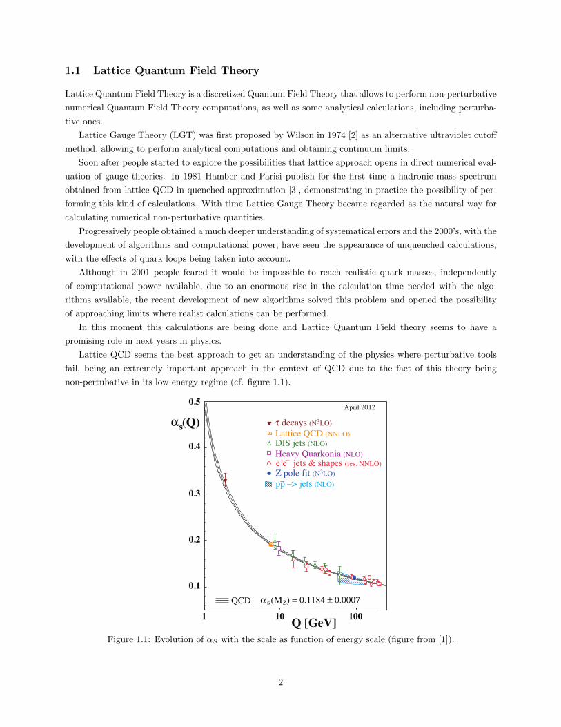
Lattice QCD seems the best approach to get an understanding of the physics where perturbative tools

fail, being an extremely important approach in the context of QCD due to the fact of this theory being

non-pertubative in its low energy regime (cf. figure 1.1).

Figure 1.1: Evolution of αS with the scale as function of energy scale (figure from [1]).

2

Spacetime Discretization

In Lattice Quantum Field Theory we want to build a theory that can evaluate the path integral directly in

a computer. As computers cannot deal with a continuous spacetime the first obvious step is to discretize it.

There are several possible approaches to this, being that the most widely used is the discretization of space

time in an isotropic hypercubic lattice with a certain lattice spacing between points. This spacing can be

determined a posteriori by the appropriate matching of lattice quantities with physical measured quantities

or can just be taken as a parameter which computed quantities depend on.

This isotropic hypercubic lattice is the simplest choice that can be taken and, although other approaches

have been tried sporadically (e.g. [4,5]), it remains the almost exclusively used discretization. This hypercube

will have dimensions NS ×NS ×NS ×NT and periodical boundary conditions in all directions1.

The next step consists in introducing the fields in the lattice in a way that they preserve the proprieties

we are interested in. This is done by considering the fermions as Grassman variables laying in the lattice

sites and the gauge fields as group elements in the links between lattice sites. So we assign the gauge field

in the links the average value of the field in between the two nearest points. We will see that this definition

allows to preserve gauge invariance.

We denote the fermions by ψ and the gauge field by Uµ (cf. figure 1.2).

μ

ν

Uμ ψ(x)

Uν

Uμ -1

Figure 1.2: Fermions and gauge fields.

Gauge invariance

It is important to preserve the gauge symmetry of the original theory. To do so we need to understand how

to build gauge invariant quantities in the lattice we just defined. First of all let us transcribe the notion of

gauge freedom to the lattice. Gauge freedom is the freedom to perform a local gauge transformation of our

fields, which can be expressed as the multiplication of a gauge element locally. In lattice a general gauge

transformation can be parametrized as

ψ(x)→ V (x)ψ(x) (1.1)

ψ(x)→ ψ(x)V −1(x) (1.2)

Uµ(x)→ V (x)Uµ(x)V −1(x+ µ) (1.3)

U−1µ (x)→ (V (x)Uµ(x)V −1(x+ µ))−1 = V (x+ µ)U−1

µ (x)V −1(x). (1.4)

We will now check an example of a gauge invariant quantity on the lattice. Let us consider a closed

product of links in the lattice, for example the smallest possible one Pµν , the plaquette, a product of four

1Again this choice is not unique. Recently there have been attempts to work with lattices that are not periodic in time [6],which allows to solve some topology related technical problems, although it is not yet well explored.

3

neighbor links (cf. figure 1.3). We have

Pµν(x) ≡ Uµ(x) Uν(x+ µ) U−1µ (x+ ν) U−1

ν (x). (1.5)

Performing a general gauge transformation we have [7]

P ′µν(x) = V (x) Uµ(x) V −1(x+ µ)V (x+ µ) Uν(x+ µ) V −1(x+ µ+ ν)×

× V (x+ µ+ ν) U−1µ (x+ ν) V −1(x+ ν)V (x+ ν) U−1

ν (x) V −1(x) =

= V (x) Uµ(x) Uν(x+ µ) U−1µ (x+ ν) U−1

ν (x) V −1(x) (1.6)

We can take the trace of P ′µν2 and use the cyclic property of the trace obtaining

Tr[P ′µν(x)

]= Tr

[V (x) Uµ(x) Uν(x+ µ) U−1

µ (x+ ν) U−1ν (x) V −1(x)

]=

= Tr[Uµ(x) Uν(x+ µ) U−1

µ (x+ ν) U−1ν (x)

]= Tr [Pµν(x)] (1.7)

so we can conclude that this quantity TrPµν is gauge invariant.

Now that we have an idea about how to get gauge invariant quantities we can do it in a more general

way. It is easy to check that when we have an ordered product of links if we perform a gauge transformation

all the transformation matrices vanish except the first and the last ones. If U(x, y; C) denotes that product

for any ordered path C starting at x and ending at y it transforms as

U(x, y; C)→ V (x)U(x, y; C)V −1(y). (1.8)

So, to get a gauge invariant we need to eliminate those transformation matrices in the edges of the path. We

have two aways to do so

• taking the beginning and the end to be the same point and take the trace of U(x, y; C) (a generalization

of our plaquette example)

Tr [U(x, x; C)]→ Tr [U ′(x, x; C)] = Tr[V (x)U(x, x; C)V −1(x)

]= Tr [U(x, x; C)] (1.9)

μ

νx

Pμν(x)

Uμ (x)

Uν (x)-1

Uμ (x+ν) -1

Uν(x+μ)

x+μ

x+ν

Figure 1.3: Plaquette.

2This trace is to be taken in group internal space, since this is the reason why the factors in Pµν don’t commute in general.

4

• taking the beginning and the end of the path to be, respectively, an antifermion and a fermion

ψ(x)U(x, y; C)ψ(y)→ ψ′(x)U ′(x, y; C)ψ′(y) = ψ(x)V −1(x)V (x)U(x, y; C)V −1(y)V (y)ψ(y)

= ψ(x)U(x, y; C)ψ(y). (1.10)

Action

We have discretized the spacetime, it is now important to understand how we can build an action in our new

theory. This choice is not unique, we can accept several actions since they respect gauge invariance and have

the right continuum limit.

The correct limit of the gauge action in continuum should be the well-known Yang-Mills action

SG = −1

4

∫d4x TrFµνF

µν . (1.11)

We can start by taking our example of the plaquette operator we defined before. We will do this in the

Abelian case, the case of most interest for us in this dissertation. The non-Abelian case is not very different

(although the calculations are somewhat lengthier and more complicated). We have

Pµν(x) = Uµ(x) Uν(x+ µ) U−1µ (x+ ν) U−1

ν (x) (1.12)

It makes sense to define

Uµ(x) ≡ eiag[Aµ(x+ µ2 )] (1.13)

once the link values are defined in the middle point of the link. This way in the new variables the plaquette

will be

Pµν(x) = eiag[Aµ(x+ µ2 )+Aν(x+µ+ ν

2 )−Aµ(x+ν+ µ2 )−Aν(x+ ν

2 )] =

= eiag[Aµ(r− ν2 )+Aν(r+ µ2 )−Aµ(r+ ν

2 )−Aν(r− µ2 )] (1.14)

where r is the coordinate of the center of the plaquette. Noting that Aµ(r− ν2 ) = Aµ(r)+∂νAµ

(−a2)

+O(a2)

we have in the exponent

iag[Aµ(r − ν

2)−Aµ(r +

ν

2) +Aν(r +

µ

2)−Aν(r − µ

2)] =

= iag[Aµ(r)− a

2∂νAµ −Aµ(r)− a

2∂νAµ +Aν(r) +

a

2∂µAν −Aν(r) +

a

2∂µAν +O(a2)] =

= iag[∂µAν − ∂νAµ +O(a2)] = ia2gFµν + iO(a3). (1.15)

Expanding now the exponential we can get

Pµν(x) = eia2gFµν+iO(a3) = 1 + ia2gFµν −

a4g2

2F 2µν + iO(a3) +O(a5). (1.16)

So the real part of plaquette contains the square of the components of the electromagnetic tensor3. This way

3Although not relevant here it is easy to check that, unlike with non-Abelian theories, in U(1) it is possible to probe theelectric field directly using the imaginary part of the plaquette.

5

we can take the action to be

Sg =1

g2

∑x

∑µ<ν

Re [1− Pµν(x)] = β∑x

∑µ<ν

Re [1− Pµν(x)] (1.17)

where we adopt the usual convention β = 1g2 .

It is easy to check that this action has as continuum limit the usual Yang-Mills action

Sg =1

g2

∑x

∑µ<ν

Re [1− Pµν(x)] =a4

2

∑x

∑µ<ν

F 2µν =

=a4

4

∑x

∑µ,ν

F 2µν −→

1

4

∫d4x FµνF

µν . (1.18)

The trace is not needed since we are working with U(1) gauge theory and U(1) group elements commute.

In a more general settlement of non-Abelian theories we would have Tr Re [1− Pµν(x)].

This action is the simplest possible and is known as Wilson action. It is possible to build many other

actions taking into account more loop contributions (e.g. [7]). Some of these actions can cancel terms in the

expansion up to higher orders, making the action converge faster to the continuum. They have although the

disadvantage of bringing more complexity and taking more time to compute.

Strong coupling expansion

We can calculate prediction of this theory in the limit of strong coupling (β → 0⇔ g →∞).

We want to calculate the average density of plaquette in this limit. This quantity is given by

〈Pµν〉 = Z−1

∫dUPµνe−S (1.19)

where S, the action, is the Wilson action we introduced before.

When β → 0, the integral ∫dUPµν e−S → 0 (1.20)

because ∫dUPµν = 0. (1.21)

Basically this reflects the fact that, in the strong coupling limit, the links values are independent of each

other so the average should be 0.

Consequently we will have ∫dUPµν P

∗αγ = δµαδνγ (1.22)

because in U(1) we have P ∗µν = P−1µν .

6

The next step is to expand the e−S in a β series

e−S = exp

[−β

(1−

∑µ<ν

RePµν

)]= e−β exp

[β∑µ<ν

RePµν

]= e−β exp

[β

2

∑µ<ν

(Pµν + P ∗µν

)]

= e−β

[1 +

β

2

∑µ<ν

(Pµν + P ∗µν

)+O(β2)

]. (1.23)

So, if we replace the action expansion in average plaquette integral, we get

〈Pαγ〉 = Z−1

∫dUPαγ e−S = Z−1

∫dUPαγ e−β

[1 +

β

2

∑µ<ν

(Pµν + P ∗µν

)+O(β2)

]=

= Z−1e−β

[∫dUPαγ +

β

2

∫dUPαγ

∑µ<ν

(Pµν + P ∗µν

)+O(β2)

]. (1.24)

For the reasons stated before the first integral evaluates to 0 and the second one to 1 so the result is

〈Pαγ〉 = Z−1e−β[β

2+O(β2)

]. (1.25)

It is easy to check that

Z =

∫dU e−S = e−β

∫dU

[1 +

β

2

∑µ<ν

(Pµν + P ∗µν

)+O(β2)

]= e−β

[1 +O(β2)

](1.26)

Z−1 = eβ[1 +O(β2)

]−1= eβ

[1−O(β2)

](1.27)

So we get

〈Pαγ〉 =β

2+O(β2). (1.28)

As in this limit the link variables become independent of each other the result does not depend on

spacetime dimension.

Monte Carlo Methods

We discretized spacetime and introduced the fields of the theory in the lattice. Now we should find a way

to compute quantities in our new theory. For that we should find a way of calculating the Feynman Path

Integral. For that usually people resort on Monte Carlo methods, in practice introducing a new layer of

discretization. The process consists in taking the path integral and discretizing it by taking into account only

a finite number of field configurations which are representative of the system in thermal equilibrium.

We start with the partition function

Z =

∫Dφ eiS[φ] (1.29)

7

and the average of an operator

〈O〉 =

∫Dφ O[φ] eiS[φ]∫Dφ eiS[φ]

. (1.30)

The next step is to effectuate a Wick rotation, in order to be in an Euclidean space.

ZE =

∫DφE e−SE [φE ] (1.31)

and

〈O〉E =

∫DφE OE [φE ] e−SE [φE ]∫DφE e−SE [φE ]

. (1.32)

where the subscript E indicates euclidean version, which we will use almost always. From now on, for the

sake of simplicity, we will drop the E subscript whenever the situation is not dubious.

This way we have

〈O〉 =

∫Dφ O[φ] P [φ] (1.33)

where

P [φ] Dφ ∝ e−S[φ] Dφ. (1.34)

Denominating a configuration for x(α), we can approximate the integral in configurations for the following

sum in Ncf configurations

〈O〉 ≈ O ≡ 1

Ncf

Ncf∑α=1

O[x(α)] (1.35)

with a correspondent standard deviation

σO =

√√√√√Var

1

Ncf

Ncf∑α=1

O[x(α)]

=

√√√√√ 1

N2cf

Var

Ncf∑α=1

O[x(α)]

= (1.36)

assuming that the configurations are independent Bienayme’s formula guarantees that we can perform the

following step4

=

√√√√ 1

N2cf

Ncf∑α=1

Var[O[x(α)]

]=

√σ2O

Ncf∝ 1√

Ncf. (1.37)

4Bienayme’s formula is a theorem that states that the variance of the sum of independent random variables is equal to thesum of the variances of those variables. For a proof check for example [8].

8

1.2 Temperature

We want to study the field at different temperatures so we need to be able to estimate it. The temperature

is given by the inverse length of the lattice in temporal direction

T (β,Nt) =1

Nta(β). (1.38)

Thus we need to introduce a scale from which we can extract the lattice spacing a. There are several

ways of doing this, the simplest one being probably the normalization to string tension. For this purpose we

study a widely used scale introduced by Sommer in 1993 [9] known as Sommer scale (r0). He argues that

this parameter has lower systematical and statistical errors than the traditional methods.

It consists of choosing a specific point in the force, taken as the derivative of the potential, and using it as

reference distance to normalize quantities. r0 is defined through the relation r20F (r0) = 1.65. Details about

our specific implementation are given in section 2.4.

1.3 Effective String Theory

Effective string theory is an effective bosonic string theory that is believed to model successfully many aspects

of confining theories. This was proposed long ago and was initially supported by two arguments [10]

• meson spectroscopy could be explained assuming a string-like interaction between quarks,

• the discovery that in strong coupling limit the interquark potential rises linearly.

Many papers were published about this subject and many predictions of effective string theory have been

studied. It predicts the formation of a flux tube between charges, giving origin to an asymptotically linear

potential, responsible by the confinement property of the theory.

Its most famous result is the shape of the confining potential in leading order [11]

V (r) = A+ σr +γ

r+O(1/r3) (1.39)

where γ = (d−2)π24 and d is the dimension of the spacetime. This potential have some striking properties

namely being independent of the gauge group we chose for the interaction. Also the numerical value of γ,

known as Luscher term, is a dimensionless constant thought to be independent of gauge group, just depending

on the dimensionality of spacetime. This fact is confirmed by many high precision studies in lattice using

different groups and spacetime dimensions [10,12–18].

Recently there have been progress in this area with the calculation of the energy spectrum of the theory

up to higher orders (e.g. [19]).

Also a well-known result of effective string theory is the evolution of string tension with temperature. A

2-loops expression for it is [20]

σ(Nt) = σ0 −(d− 2)π

6N2t

− (d− 2)2π2

72σ0N4t

(1.40)

where σ0 is the value of string tension at zero temperature.

9

Other important results of this theory are the predictions about the width of the flux tube. The theory

predicts that the flux tube width should increase logarithmically with the distance between the sources at

zero temperature and linearly at high temperature at leading order [20]

• zero temperature w2lo(r/2) = d−2

2πσ log( rρ0 )

• finite temperature w2lo(r/2) = d−2

2πσ log Nt4ρ0

+ d−24Ntσ

r +O(e−2πr/Nt)

where Nt is the temporal extent of the lattice, d is the dimension of spacetime and ρ0 is some distance scale

to be fitted.

These expressions have been recently shown [21,22] to be correspondingly the low and high temperature

limits of the same expression that incorporates the dependence of temperature explicitly

w2lo(r/2) =

d− 2

2πσlog

(r

ρ0

)+d− 2

πσlog

(η(2iu)

η2(iu)

)(1.41)

where η is Dedekind η function and u = Nt2r incorporates the temperature dependence.

This width is calculated in the lattice through the computation of

w2(r/2) =

∫dx⊥x

2⊥O(x⊥)∫

dx⊥x2⊥

(1.42)

where O(x⊥) is an operator that represents the flux tube (e.g. the density of energy) and the integral is

evaluated in the mediator plane of the charges.

10

Chapter 2

Methods

We describe the numerical methods used to obtain our results.

2.1 Generation of configurations

We want to generated a set of configurations which should be decorrelated of each other (ideally independent),

so we can guarantee that our estimate for the error is correct.

We define the autocorrelation of configurations as

C(x(a), x(b)) =1

V × d

∣∣∣∣∣∑x

∑µ

[U (a)µ (x)

]−1

U (b)µ (x)

∣∣∣∣∣ . (2.1)

Errors estimation

We use Jackknife method for error estimation. This method was introduced in 1956 by Quenouille [23] and

two years latter by John Tukey [24].

It provides a method for estimating the variance of a general unknown distribution. It consists in sys-

tematically taking points out of the average and checking how much does it change, relating this change to

the variance of the distribution.

If we have a dataset with N measurements of an observable x with average x we define xj = 1N−1

∑i 6=j xi

(the average extracting the measurement j). So for the variance of the average x we have the following

expression [25]

σ2x ≡

N − 1

N

N∑i=1

(xj − x)2

(2.2)

It can also be generalized to a method in which the data is group in bins of a certain size, where an

appropriate choice of bin sizes allows to solve the problems related to the absence of statistical independence

between consecutive measurements.

Initial configuration

We implement two possible initial configurations: one with all gauge elements aligned (known as cold start)

and one for which the group elements are drawn from an uniform random distribution (known as hot start).

11

If enough updates are applied they should produce identical results, converging to the set of states that

characterizes the thermal equilibrium to the chosen β.

Metropolis algorithm

Metropolis algorithm is a Monte Carlo algorithm that allows to draw samples from a probability distribution.

It produces a Markov chain of lattice configurations when applied sequentially to an initial configuration.

It is a simple algorithm that consists in the following procedure [26]:

• generate a new random link θnew with uniform probability within the group

• if the action of the new link decreases accept it automatically, otherwise accept it with probability

e−Snew/e−Sold .

An alternative to this is the Heat-bath algorithm. The difference is that instead of generating a new

element with uniform probability it generates it using e−S as weight and always accepts the new element

(since it is already distributed according to the right distribution). This method has several advantages,

namely smaller correlation times due to always accepting the new element, but in U(1) it is not possible to

implement a pure Heat-bath algorithm1, although some variations that approximate this method are possible

(e.g. [27]).

Overrelaxation

In some regions of β pure Metropolis method exhibits a long autocorrelation time between configurations (cf.

figure 2.2). Because of that the need for a method which decorrelates faster becomes important.

Overrelaxation is a widely used method for this propose. It was first introduced by Stephen Adler in

1981 [28, 29]. It decorrelates the system faster without changing the value of the action (so it changes a

configuration to a different one which has equal probability of occurrence). There are several variations on

this method, all of them having the same base idea.

The one we implement corresponds in practice to a reflection of the value of the links in relation to the

minimum action (cf. figure 2.1) so

eiθ → ei(θmin+(θmin−θ)) = ei(2θmin−θ) (2.3)

where θmin is to the phase that would minimize the action given fixed links around it. As Wilson action is

symmetric for reflections about its minimum this change keeps the action constant. We implement this by

applying overrelaxation to a direction at a time keeping the others constant.

The minimum link that minimizes the action can be easily calculated.

Sµ = β∑ν 6=µ

(1− Re

[eiθµν

])= 6β − β Re

∑ν 6=µ

eiθµν

= 6β − β Re

eiθµ∑ν 6=µ

ei(θµν−θµ)

= (2.4)

1For constructing a heat-bath algorithm we should integrate and invert dp(U) = dUe−S . Developing dp(U) = dUe−S we getto dp(θ) ∝ eβ|Wµ| cos(θ)dθ which integral can not be written as a closed form. The alternative is to use numerical approximationsof this method, which can get results close to a pure heat-bath method.

12

Re

Im

θold

θminθnew

Figure 2.1: Reflection of the phase in overrelaxation method, conserving the action constant.

factorizing the staple

= 6β − βRe[eiθµWµ

]= 6β − β|Wµ|Re

[ei(θµ−θt)

]= 6β − β|Wµ| cos(θµ + θt) (2.5)

Now we can find the θµ that minimizes the action.

dSµdθµ

∣∣∣∣θµmin

= 0⇒ sin(θµmin + θt) = 0⇔ θµmin = −θt + kπ (2.6)

Replacing in the previous expression for overrelaxation we obtain

eiθ → ei(−2θt−θ+2kπ) ⇔ θ → −2θt − θ + 2kπ. (2.7)

The freedom of choosing k value reflects the periodicity of the action and ensures we can project the result

in our [−π, π] working interval.

This method decorrelates configurations much faster than using metropolis method alone (cf. figure 2.2

and figure 2.3).

0

0.2

0.4

0.6

0.8

1

0 500 1000 1500 2000

corr

elat

ion

iterate

no overrelaxation1 overrelaxation step

Figure 2.2: Correlation of configurations in function of number of updates, with and without the use ofoverrelaxation method, for a lattice with β = 4 and volume 244.

13

0.0001

0.001

0.01

0.1

1

0 5 10 15 20 25

corr

elat

ion

iterate

no overrelaxation1 overrelaxation step

2 overrelaxation steps3 overrelaxation steps

Figure 2.3: Correlation of configurations in function of number of updates, for different amount of overrelax-ation steps, for a lattice with β = 4 and volume 244.

2.2 Multihit

A technique frequently applied to reduce the statistical error is multihit. It consists in a replacement of

the links in time direction with effective links calculated through an average process against a constant

background.

This new variables have the same average of the old links but a smaller variance so they have smaller

statistical errors than the traditional links. Most of the times this average is evaluated stochastically, but in

U(1), as we will see, this substitution can be easily done analytically. This analytical process is frequently

referred to as link integration.

The procedure corresponds to the following substitution [30,31]

Uµ(x)→∫

dUU exp(−βS)∫dU exp(−βS)

=I1(β|Wµ(x)|)I0(β|Wµ(x)|)

Wµ(x)

|Wµ(x)|(2.8)

where I0 and I1 are the modified Bessel functions of order 0 and 1 and Wµ(x) is the sum of the staples of

the Uµ(x) link. If calculating correlations between links in the same temporal layer, they should be spaced

of at least two lattice spacings to ensure the result is correct.

The general formula for modified Bessel functions of type 1 is

Iα(x) =1

π

∫ π

0

exp [x cos(θ)] cos(αθ)dθ − sin(απ)

π

∫ ∞0

exp(−x cosh t− αt)dt. (2.9)

So, in particular,

I0(x) =1

π

∫ π

0

exp [x cos(θ)] dθ (2.10)

and

I1(x) =1

π

∫ π

0

exp [x cos(θ)] cos(θ)dθ. (2.11)

14

Now we should rewrite the action in a good way for our purpose

S = β∑ν 6=µ

(1− Re

[eiθµν

])= 6β − βRe

∑ν 6=µ

eiθµν

= 6β − βRe

e−iθµ∑ν 6=µ

ei(θµν+θµ)

=

we can factorize the staple

= 6β − βRe[e−iθµWµ

]= 6β − β|Wµ|Re

[ei(−θµ+θt)

]= 6β − β|Wµ| cos(θµ − θt)

Then we should rewrite the integrals in multihit expression in terms of the modified Bessel function∫dUUµe−S =

∫ π

−π

dθ

2πeiθe−6βeβ|Wµ| cos(θ−θt) =

e−6β

2π

∫ π+θt

−π+θt

dθ′ei(θ′+θt)eβ|Wµ| cos θ′

where we performed a change of integration variable θ → θ′+θt. We can change the interval [−π−θt, π−θt[

into [−π, π[ again since the integrand has period 2π

=e−6βeiθt

2π

∫ π

−πdθ′eiθ

′eβ|Wµ| cos θ′ =

e−6βeiθt

2π

∫ π

−πdθ′ (cos θ′ + i sin θ′) eβ|Wµ| cos θ′ =

the part of the integrand proportional to cos θ′ is even and the part proportional to sin θ′ is odd and they are

integrated in a symmetric interval around the origin so

= e−6βeiθt1

π

∫ π

0

dθ′ cos θ′eβ|Wµ| cos θ′ = e−6β Wµ

|Wµ|I1(β|Wµ|)

where we took into account that eiθt =Wµ

|Wµ| and 1π

∫ π0

dθ′ cos θ′eβ|Wµ| cos θ′ = I1(β|Wµ|).

The second integral can be obtained with equivalent calculations to be∫dUe−S =

∫ π

−π

dθ

2πe−6βeβ|Wµ| cos(θ−θt) =

e−6β

2π

∫ π+θt

−π+θt

dθ′eβ|Wµ| cos θ′ (2.12)

= e−6β 1

π

∫ π

0

dθ′eβ|Wµ| cos θ′ = e−6βI0(β|Wµ|). (2.13)

So we get the final result

Uµ(x)→∫

dUU exp(−S)∫dU exp(−S)

=e−6β

e−6β

I1(β|Wµ(x)|)I0(β|Wµ(x)|)

Wµ(x)

|Wµ(x)|=I1(β|Wµ(x)|)I0(β|Wµ(x)|)

Wµ(x)

|Wµ(x)|. (2.14)

2.3 Luscher-Weisz Multilevel

Multilevel algorithm was purposed by Martin Luscher and Peter Weisz in 2001 [32] as a method for achieving

exponential error reduction in some lattice gauge theory calculations. It is useful when the lattice is in

confining phase and a local action is used, especially for evaluating average values of Polyakov or Wilson

15

loops.

Method

This method is inspired on the multihit method and explores the locality of the action by factorizing the

path integral into smaller integrals calculated over sublattices. We will follow Luscher and Weisz’s paper [32]

in this section, focusing on Polyakov loop, since it is the structure we are most interested in our work, and

applying it to U(1) group.

We will start by introducing two-link operators since they play an essential in the formulation of the

theory. Two-link operators are structures defined from the tensor product of two links in the same time layer

at a certain distance r (cf. figure 2.4). This structure represents the propagation in time of a pair of fermions

from time t to time t+ 1 and they can be regarded as the basic constituents of the Polyakov loop correlation

or of the temporal part of Wilson loop. They are defined as the following

T(x, t, r, µ) = U∗0 (x+ t0) U0(x+ t0 + rµ). (2.15)

We can note that this structure would be much more complicated in non-Abelian theories, since although in

U(1) the tensor product reduces to the usual product of two complex numbers this is not the case in general.

Now we can rewrite the Polyakov loop correlation in terms of these newly defined variables

P (x)∗P (x+ rµ) =(U0(x)...U0(x+ T 0)

)∗ (U0(x+ rµ)...U0(x+ T 0 + rµ)

)=

= T(x, 0, r, µ)...T(x, t, r, µ)...T(x, T, r, µ). (2.16)

Next we will see how we can break the Polyakov loop correlation written like this in a product of averages

over sublattices.

To do so we need to find a way of isolating sublattices from within our lattice. These sublattices are

time-slices of our original lattice, contained between two hyperplanes of constant time x0 and y0. If we take

two of those hyperplanes and hold their spatial links constant we can isolate the dynamics of the sublattice

from the rest. This can be done thanks to the locality of the action (because the action only depends on

plaquettes adjacent to it). This way we can calculate subaverages of quantities inside the smaller lattice.

We follow the usual convention and denote the sublattice expectation values with square brackets [...] and

expectation values over the whole lattice as 〈...〉.

μ

0

P(x)

U0 (x+r+x0) -1U0(x+x0)

t = 0

t = T

r

T(x,r,x0)

x

Figure 2.4: Two-link operator, as part of a Polyakov loop.

16

It is now possible to separate the integral in a hierarchical integration process with several intermediate

levels. This integrals satisfy identities like [T(x, t)T(x, t+ 1)] = [[T(x, t)][T(x, t+ 1)]], so for example we can

calculate the average of the Polyakov loop correlation like this

〈P ∗P 〉 = 〈[[T(x, t)][T(x, t+ 1)]][[T(x, t+ 2)][T(x, t+ 3)]]...[[T(x,Nt − 2)][T(x,Nt − 1)]]〉. (2.17)

It is easy to check that the innermost average corresponds to a multihit process because it fixes the spatial

links everywhere and averages the link. This way the multilevel algorithm can be seen as a generalization of

multihit.

Polyakov loop correlation

0

4

8

t

x

T(2)(x,0,r)

x x+r

T(2)(x,2,r)

T(2)(x,4,r)

T(2)(x,6,r)

Figure 2.5: Multilevel method for Polyakov

loop correlations.

For calculating Polyakov loop correlation is useful to introduce

some auxiliary quantities that will be averaged in the sublat-

tices.

Here we follow approximately the notation defined in [31].

We start by defining the operator

T(2)(x, t, r, µ) = T(x, t, r, µ)T(x, t+ 1, r, µ). (2.18)

If we define the first average as an average in sublattices of

thickness 2 we have Polyakov loop correlation

〈P ∗P 〉 = 〈[T(2)(x, 0, r, µ)][T(2)(x, 2, r, µ)]...[T(2)(x,Nt − 2, r, µ)]〉.(2.19)

In our code we implemented one more level in order to achieve

a further reduction on errors, calculating

〈P ∗P 〉 = 〈[[T(2)(x, 0, r, µ)][T(2)(x, 2, r, µ)]]...[[T(2)(x,Nt − 4, r, µ)][T(2)(x,Nt − 2, r, µ)]]〉.(2.20)

In practice the algorithm proceeds in a nested scheme as follows

17

Repeat level 0 process n0 times; average the results (〈P ∗P 〉)

Level 0

Update the whole lattice k0 times

Repeat level 4 process n4 times; average the results ([[T(2)][T(2)]])

Level 4

Update the lattice k4 times freezing spacial links in layers with t multiple of 4

Repeat level 2 process n2 times; average the results ([T(2)])

Level 2

Update the lattice k2 times freezing spacial links in layers with t multiple of 2

Calculate T(2)

Calculate [T(2)][T(2)]

Calculate P ∗P

Electromagnetic Field

In section 1.1 we saw how to expand the plaquette

Pµν = eia2gFµν+iO(a3) = 1 + ia2gFµν −

a4g2

2F 2µν + iO(a3) +O(a5). (2.21)

It follows that we can measure electromagnetic field tensor components through the study of the imaginary

part of the plaquette operator

ImPµν = a2gFµν +O(a3). (2.22)

Since g = 1/√β we have

a2Fµν =√β ImPµν +O(a3). (2.23)

Similarly if we want to study the squared electromagnetic field we can take the real part of the plaquette

a4F 2µν = 2β (1− RePµν) +O(a6). (2.24)

We want to study the field produced by static charges at a certain distance of each other so we should

correlate our operator with a Polyakov loop correlation representing those charges, getting

〈O〉P∗P =〈P ∗PO〉〈P ∗P 〉

− 〈O〉 (2.25)

where O stands for any operator we want to measure and 〈O〉P∗P stands for the expectation value of O

18

produced by the charges represented by P ∗P .

0

4

8

t

x

TO(2)(x,x0,0,r)

x x+r

T(2)(x,2,r)

T(2)(x,4,r)

T(2)(x,6,r)

0

4

8

x x+r

T(2)(x,2,r)

T(2)(x,4,r)

T(2)(x,0,r)

+ ... +

O(x,0)

O(x,7)

TO(2)(x,x0,6,r)

Figure 2.6: Multilevel method for electromagnetic field.

To implement a multilevel algorithm for this calculation it is useful to introduce some more quantities,

besides T and T(2),

TO(2)(x0, x, t, r, µ) = [T(x, t, r, µ)T(x, t+ 1, r, µ)O(x0, t) + T(x, t, r, µ)T(x, t+ 1, r, µ)O(x0, t+ 1)] (2.26)

T(4)(x, t, r, µ) = [T(2)(x, t, r, µ)][T(2)(x, t+ 2, r, µ)] (2.27)

TO(4)(x0, x, t, r, µ) = [T(2)(x, t, r, µ)][TO(2)(x0, x, t+ 1, r, µ)] + [TO(2)(x0, x, t, r, µ)][T(2)(x, t+ 1, r, µ)].

(2.28)

With this notation we can write

〈P ∗(0)P (rµ)O(x0)〉 =1

NdSNtd

∑x

∑µ

[

[ TO(4)(x0, x, 0, r, µ)T(4)(x, 4, r, µ)...T(4)(x,Nt − 4, r, µ) +

+ T(4)(x, 0, r, µ)TO(4)(x0, x, 4, r, µ)...T(4)(x,Nt − 4, r, µ) + ...

... + T(4)(x, 0, r, µ)T(4)(x, 4, r, µ)...TO(4)(x0, x,Nt − 4, r, µ)] (2.29)

which can be calculated in a way analog to the Polyakov loop correlation.

2.4 Sommer scale

As stated before, we use Sommer r0 to establish a scale in the lattice.

To determine it we interpolate a function F (r) = f1 + f2r2 which constitutes a good local approximation

to the force [9]. To do so we compute the force F (rr) = V (r) − V (r − 1), as a discretized derivative of the

19

potential and numerically solve the system

f1 +f2

r2r

= V (r)− V (r − 1) (2.30)

f1 +f2

r2r+1

= V (r + 1)− V (r) (2.31)

r20

(f1 +

f2

r20

)= 1.65 (2.32)

to obtain the r0 value. The value of rr is chosen to be a tree-level improved variable as to eliminate the

O(a2) term from r0. This is done choosing the value of [9]

rr =

[4πG(r)−G(r − d)

d

]−1/2

(2.33)

G(r) =1

4a

∫ π

−π

d3k

(2π)3

cos(k1r/a)

4∑3j=1 sin2(kj/2)

. (2.34)

This definition yields a considerable improvement for small r0 over choice of rr = r+ a2 , but becomes negligible

at bigger values since the force becomes constant.

Having determined r0(β) = r0/a(β) scale we can use it to estimate the temperature at which we are

working. Since the temperature is

T =1

Nt a(β). (2.35)

From here we can easily get

T (β,Nt)

Tc=Ntc a(βc)

Nt a(β)=Ntc r0(β)

Nt r0(βc)(2.36)

where Tc is the reference critical temperature for confining phase transition.

2.5 CUDA

CUDA (Computer Unified Device Architecture) is a computer architecture developed by NVIDIA that allows

to explore the graphics processing units (GPU’s) for general purpose calculations. We use CUDA extensions

of C++ programming language, which consist a set of extensions for this language that allow to use many

features of C++, like classes and templates in GPU calculations.

Due to the challenges faced by graphics processing, GPU architecture have evolved into devices extremely

well suited for highly parallelized code execution, with many cores and high memory bandwidth. This is ideal

for lattice QCD calculations, because this calculations typically involve the analysis of all points of lattice

independently which results in highly parallelizable calculations.

We use NVIDIA Fermi generation GPU’s that support double precision operations and allow the necessary

performance for our calculations.

For our calculations we resorted mainly to four GPU’s, two NVIDIA GeForce GTX 580 and two NVIDIA

Tesla C2075 (specifications can be found in table 2.1).

20

GeForce GTX 580 [33] Tesla C2075 [34]CUDA capability 2.0 2.0Multiprocessors (MP) 16 14Cores per MP 32 32Total number of cores 512 448Global memory 3072 MB GDDR5 6144 MB GDDR5Shared memory (per SM) 48 KB or 16 KB 48 KB or 16 KBL1 cache (per SM) 16 KB or 48 KB 16 KB or 48 KBL2 cache (chip wide) 768 KB 768 KBClock rate 1.57 GHz 1.15 GHzMemory Bandwidth 192.4 GB/s 144 Gb/sDevice with ECC support no yes

Table 2.1: Specifications of the GPU’s used in this work.

Code implementation

For the configurations we store each lattice link in the form of a phase θ, so we store one double precision

floating point number per lattice link. This away of storing has several advantages, namely being always

projected in U(1) circle and mapping multiplications of group elements to sums of the phases (eiθ1 × eiθ2 =

ei(θ1+θ2). Whenever we need to have sums or operations that fall out of the U(1) group in general (e.g. when

we apply multihit), we store the numbers in the complex form a+ ib, thus using 2 double precision floating

point numbers.

CUDA organizes the parallel threads into calls of kernels, organized in a grid of blocks, which are executed

in parallel in arbitrary order. To each thread CUDA assigns a threadId and a blockId that uniquely identify

the thread. With these ID’s we compute the position of the thread as a set of four lattice indices, corresponding

to a position in the four directions of spacetime. The CUDA version we use, CUDA 4.1, allows the use of

3D indices in both grids and blocks, so in 4D kernels we use the first index to encode x and y directions, the

second to z and the third to t.

As the threads are not guaranteed to run in any specific order we should ensure that the different calls

do not threads do not interfere with each other. For that purpose, whenever we run update operations on

lattice that depend only on neighbor sites (e.g. Metropolis or overrelaxation updates), we separate the calls

in odd and even points (when the sum x+ y+ z+ t is odd or even). This way we can update the odd points,

running all the directions, synchronize, and update the even points, running all the directions again, making

sure they keep independent.

Whenever the operations depend only on reading the lattice, thus not interfering with each other, we

calculate all the lattice points at the same time (e.g. calculating plaquette or Polyakov loop, that only

perform reading operations in the lattice).

To calculate averages we resort to a reduction algorithm that sums all the points in a lattice. We use an

implementation based on the one provided in NVIDIA SDK (for documentation check [35]).

CUDA has access to several kinds of memory, which should be well managed to optimize the program.

The NVIDIA FERMI memory architecture is summarized in figure 2.7.

For optimizing the memory accesses whenever we need to effectuate read-only operations on a configura-

tion, we store it in texture memory, which is global memory but has a special memory cache that optimizes

this kind of accesses.

Multilevel algorithm requires a large amount of memory because we should store the correlations of the

21

Figure 2.7: CUDA memory architecture.

T(2) and T(4) operator with the plaquette for all the space points. This way for each point we want to test

the field we should store N3sNt (lattice volume) ×3 (spacial directions) /n (time-like links are grouped into

sets of n) ×2× size of double. For a 244 with two levels (2 and 4) lattice it yields approximately 11.4 Mb per

point where we wish to calculate the field.

2.6 Other computational resources

Although our lattice code is completely written in CUDA, we make use of Mathematica and qtiplot for fits,

numerical integrations, and some other general purpose calculations, as well as, of Mathematica and gnuplot

for plotting and creating the figures presented in this work.

22

Chapter 3

Results

In this chapter we state and analyze the main results obtained in our studies.

3.1 Average plaquette density

Average plaquette density is known to have a phase transition, known as bulk transition, which corresponds

to a transition in the lattice spacing a.

This phase transition can be clearly observed as a peak in plaquette susceptibility (〈P 2µ〉 − 〈Pµ〉2) (cf.

figure 3.1).

0

5e-05

0.0001

0.00015

0.0002

0.00025

0.0003

0 0.5 1 1.5 2

Pla

quet

tesu

scep

tibili

ty

β

Figure 3.1: Plaquette susceptibility with β in a 4D 84 lattice.

We study 1 − 〈Pµν〉 which is the quantity most often studied in literature instead of 〈Pµν〉. We present

our results for several spacetime dimensions (cf. figure 3.2). We can verify that they follow the expected

limits in strong and weak coupling regimes. We find that the phase transition details depend significantly on

the dimension of spacetime, maybe even changing the order of phase transition.

Our results for plaquette reproduce the results that can be found in many publications.

3.2 Confining phase transition

Confining/non-confining transition can be studied through the analysis of different parameters. The best

parameter to study this are Polyakov loop expectation value or plaquette susceptibility. Polyakov loop

23

0

0.2

0.4

0.6

0.8

1

0 1 2 3 4 5 6

1-<P

>

β (a)

0

0.2

0.4

0.6

0.8

1

0 0.5 1 1.5 2 2.5 3

1-<P

>

β (b)

0

0.2

0.4

0.6

0.8

1

0 0.5 1 1.5 2

1-<P

>

β (c)

0

0.2

0.4

0.6

0.8

1

0 0.2 0.4 0.6 0.8 1 1.2 1.4

1-<P

>

β (d)

Figure 3.2: Average plaquette density in function of β for 2D (a), 3D (b), 4D (c) and 5D (d). The error barsare much smaller than the size of the points in the graph. The functions plotted are the strong and the weakcoupling limits calculated for the theory. The vertical line corresponds to βc extracted from Polyakov loopexpectation value. 24

expectation value is 0 in confining phase and rises fast after the phase transition, making it possible to use

it as an order parameter for this phase transition.

We calculated Polyakov loop expectation value to identify with precision the location of the phase tran-

sition in the lattice sizes we use (typically 244). Our results are presented in the following tables and graphs.

This transition is more obvious on smaller lattices so we chose a 84 lattice to illustrate it (cf. figure 3.3).

0

0.1

0.2

0.3

0.4

0.5

0.6

0 0.5 1 1.5 2

Pol

yako

vlo

op

β

Figure 3.3: Polyakov loop expectation value with β in a 4D 84 lattice (the error bars are smaller than thesize of the points).

3.3 Sommer scale

We use Sommer r0 to establish a scale in the lattice so we can determine the temperature.

We obtain the error in r0 by averaging the results of the difference of the result with the interpolation

including an extra term of order 1/r4.

We study the temperature normalized to critical temperature at each the system becomes unconfined.

In order to determine it we first had to estimate the critical temperature. We determined the plaquette

susceptibility (cf. figure 3.4) and fitted the peak of phase transition in a system with Nt = 4. We obtained

the approximate value of βc = 1.003 and r0/a(βc) = 9.10 ± 0.97, which yields for critical temperature

Tc ≈ 2.3r0.

0

5e-06

1e-05

1.5e-05

2e-05

2.5e-05

3e-05

0.9 0.95 1 1.05 1.1

<P2 >-

<P>2

β

Figure 3.4: Plaquette susceptibility in function of β in a lattice 243 × 4.

25

Then we calculated the temperatures for β = 1 and Nt in the range of 4 to 24. To estimate the error in

temperature we extrapolated the error induced by the error in critical temperature, since this was calculated

close to the phase transition having a significantly bigger error than the other temperatures.

Our results for both r0 and temperature are stated in table 3.1.

Nt r0/a T/Tc04 3.60 ± 0.02 0.40 ± 0.0408 2.898 ± 0.003 0.16 ± 0.0212 2.882 ± 0.004 0.11 ± 0.0116 2.87 ± 0.02 0.079 ± 0.00820 2.86 ± 0.04 0.063 ± 0.007

Table 3.1: Dependence of r0/a and temperature with Nt.

We can see that the r0/a grows with β which is in agreement with our expectations of lattice spacing

getting smaller with β.

3.4 Multilevel convergence

The multilevel parameters should be tuned to obtain better results. The number of necessary iterates grows

exponentially with the interquark distance [32], in order to compensate the exponential growing of the relative

error in Polyakov correlations (due to exponential decay of Polyakov correlations). To illustrate this we show

the behavior of Polyakov loop correlation with the number of multilevel iterates for different distances (figure

3.5). It is clear from the figure that the Polyakov loop correlations fall exponential with the distance as well

as that the number of multilevel iterates to obtain a stable results grow in an approximately exponential way

too.

1e-20

1e-15

1e-10

1e-05

1

1 10 100 1000 10000

<PP

* >

iterate

R = 1R = 2R = 3R = 4R = 5R = 6R = 7

Figure 3.5: Polyakov loop correlation convergence with multilevel iterate.

3.5 Potential

Static potential can be obtained through the study of Polyakov loop since we have

〈P ∗(0)P (r)〉 = e−NtV (r). (3.1)

26

This way we have

V (r) = − 1

Ntln [〈P ∗(0)P (r)〉] . (3.2)

Zero temperature

We computed the static charge potential with several values of β with and without multilevel. For the

confining phase we obtain values compatible with the potential described by effective string theory, for the

non-confining phase we obtain an 1/r dipole potential.

For β = 1.00, in the confining phase, we calculate the potential from 100 multilevel configurations, each one

with 100 level 4 and 1000 level 2 multilevel iterates, with multihit method for further error reduction (except

for r/a = 1). We fit the results (figure 3.6) and extract a value for string tension of σ = 0.16719± 0.00030,

if we force the Luscher term to be constant (χ2/dof = 0.140). With Luscher term as a fit parameter we

obtain σ = 0.1666± 0.0022 and Luscher term 0.274± 0.061 (χ2/dof = 0.147), in a good agreement with the

expected value of π/12 = 0.2618. We do not include the first two points in the fit.

0

0.2

0.4

0.6

0.8

1

1.2

1.4

1.6

1.8

2

1 2 3 4 5 6 7 8

aV

(r/a

)

r/aFigure 3.6: Potential of two static charges at β = 1. The error bars are much smaller than the size of thepoints in the graph.

For β = 3.00, now in the non-confining phase, we can observe the string tension going to zero. Multilevel

is not needed in this region since the results are numerically much more stable. We use 1000 configurations,

10 iterates away from each other, and obtain the results in figure 3.7. From the fit we extract the values of

σ = −0.000194± 0.000019 and for the coefficient of the term in 1/r 0.03468± 0.00062 (χ2/dof = 0.526).

From the potential fits we can extract the value of the string tension σ in function of β (cf. figure 3.8).

We can observe the string tension going to zero at deconfining phase transition. We extract also the value of

Luscher term which is compatible with the expected value in the confining phase of π/12 (cf. figure 3.9).

27

0

0.02

0.04

0.06

0.08

0.1

2 4 6 8 10 12

aV

(r/a

)

r/aFigure 3.7: Potential of two static charges at β = 3. The error bars are much smaller than the size of thepoints in the graph.

β b σ χ2

0.960 0.46± 0.24 0.374± 0.012 0.2010.970 0.37± 0.12 0.3336± 0.0059 0.06250.980 0.32± 0.10 0.2878± 0.0046 0.1130.990 0.319± 0.071 0.2313± 0.0030 0.04710.995 0.25± 0.15 0.2046± 0.0057 0.3351.000 0.274± 0.061 0.1666± 0.0022 0.1471.005 0.260± 0.063 0.1273± 0.0026 0.03151.010 0.265± 0.032 0.0557± 0.0011 0.0002931.0105 0.2344± 0.0029 −0.00095± 0.00013 0.007991.011 0.2291± 0.0047 −0.00122± 0.00021 0.02451.012 0.2194± 0.0070 −0.00138± 0.00031 0.1131.013 0.2139± 0.0074 −0.00140± 0.00032 0.1601.015 0.1947± 0.0049 −0.00106± 0.00016 0.03491.020 0.1896± 0.0089 −0.00133± 0.00038 0.8221.030 0.1641± 0.0043 −0.00084± 0.00014 0.2381.050 0.1478± 0.0035 −0.00073± 0.00011 0.3201.100 0.1276± 0.0025 −0.000617± 0.000082 0.6161.500 0.0794± 0.0021 −0.000422± 0.000061 0.4012.000 0.0543± 0.0017 −0.000280± 0.000052 0.6832.500 0.0420± 0.0013 −0.000222± 0.000039 0.6333.000 0.03468± 0.00062 −0.000194± 0.000019 0.5265.000 0.02001± 0.00025 −0.0001120± 0.0000081 0.254

Table 3.2: Fit parameters of potential of two static charges at different β. The fit function is V (r) =A+ b/r + σr.

28

-0.05

0

0.05

0.1

0.15

0.2

0.25

0.3

0.35

0.4

0.96 0.98 1 1.02 1.04 1.06

σ

βFigure 3.8: Dependence of string tension with β in 4D.

0.5

1

1.5

2

2.5

3

0.96 0.98 1 1.02 1.04 1.06

b

β

Figure 3.9: Dependence of 1/r term with β in 4D (normalized to π/12).

29

Finite temperatureNt σ

4 0.126± 0.004

8 0.1893± 0.0001

12 0.198± 0.003

16 0.204± 0.007

20 0.203± 0.006

24 0.205± 0.006

Table 3.3: σ in function of Nt for

β = 1.00.

Also we calculated the potential with smaller temporal lattice extents.

These graphs are analogous to the presented for Nt = 24. Our results are

in table 3.3. It is interesting to verify that these results follow closely the

theoretical prediction of effective string theory for the evolution of string

tension with Nt (cf. figure 3.10).

0

0.05

0.1

0.15

0.2

0.25

0 4 8 12 16 20 24

σ

Nt

Figure 3.10: σ extracted from potential fit at β = 1.00 for different Nt values. The curve is the theoretical

expectation from Effective String Theory at 2-loops (χ2 = 0.006). Notice that the expression is not fitted,

since the only parameter (σ0) is fixed by zero temperature result.

3.6 Flux tube profile

We calculated the Ex tube profile in the middle plan between the charges

using 100 multilevel configurations1.

To the result we fit the ansatz suggested in [20]

〈P ∗P Fµν〉〈P ∗P 〉

= A exp(−x2⊥/s)

1 +B exp(−x2⊥/s)

1 +D exp(−x2⊥/s)

. (3.3)

As expected we can notice that the flux tube (figures 3.11 and 3.12) gets broader at bigger charge

separations. In the next section (3.7), we quantify this result through the calculation of the flux tube width.

1These results were presented at Excited QCD 2012 International Meeting. For the corresponding proceeding check [36].About the width of the flux tube the results we present are an improvement over the ones since now we went to r/a = 8, insteadof just 6, and we calculated the flux tube width using 〈E2 +B2〉, instead of the 〈E2

x〉 presented at the conference.

30

-0.05

0

0.05

0.1

0.15

0.2

0.25

0.3

0.35

0.4

0 1 2 3 4 5 6

a2E

x

r/a

R = 2R = 4R = 6

Figure 3.11: Flux tube profile for several charge distances at β = 1.00 and Nt = 24 (T = 0.053Tc).

0

0.1

0.2

0.3

0.4

0.5

0 1 2 3 4 5 6

a4(E

2+

B2 )

r/a

R = 2R = 4R = 6

Figure 3.12: Flux tube profile for several charge distances at β = 1.00 and Nt = 4 (T = 0.40Tc).

31

3.7 Flux tube width

We integrate 〈E2 +B2〉 ansatz fits to calculate the flux tube width. The errors are estimated using a jackknife

algorithm.

Although the data confirms the theoretical expression for flux tube width from Effective String Theory σ

extracted from these is not compatible with the value of σ obtained from the potential.

We study field width for several temperatures, corresponding to Nt = 4, 8, 12, 24 (cf. results table 3.4).

Nt T/Tc a2σ ρ0/a χ2/dof R a2w2(r/a)

24 0.053 0.268± 0.044 0.50± 0.16 0.27

2 1.61± 0.134 2.54± 0.156 2.98± 0.138 3.22± 0.16

12 0.11 0.18367± 0.00092 0.7590± 0.0068 0.000026

2 1.68± 0.164 2.88± 0.156 3.60± 0.388 4.16± 0.82

8 0.16 0.2008± 0.0069 0.693± 0.030 0.16

2 1.68± 0.104 2.80± 0.136 3.42± 0.238 4.26± 0.29

4 0.40 0.153± 0.019 0.52± 0.17 0.30

2 2.67± 0.784 4.63± 0.156 6.66± 0.528 7.900± 0.066

Table 3.4: Widths and fit parameters of the width expression.

We can realize that the flux tube width consistently grows with the charge separation. We studied

several temperatures in order to observe the transition between the zero temperature limit (pure logarithmic

dependence) and the high temperature regime (pure linear behavior). To make the transition more obvious

we show repeated plots in logarithmic and linear scale (cf. figure 3.13).

32

0.0 0.5 1.0 1.5 2.0

1.0

1.5

2.0

2.5

3.0

3.5

2 4 6 8

1.0

1.5

2.0

2.5

3.0

3.5

(a)

0.0 0.5 1.0 1.5 2.0

1

2

3

4

5

2 4 6 8

1

2

3

4

5

(b)

0.0 0.5 1.0 1.5 2.0

1

2

3

4

2 4 6 8

1

2

3

4

(c)

0.0 0.5 1.0 1.5 2.0

2

3

4

5

6

7

8

2 4 6 8

2

3

4

5

6

7

8

(d)

Figure 3.13: Squared width in function of charge separation for 24 (a), 12 (b), 8 (c) and 4 (d). The figureson the left are plots of a2w2(r/a) vs log(r/a) and on the right a2w2(r/a) vs r/a.

33

3.8 Field in finite temperature

Field in finite temperature is numerically more stable than in zero temperature allowing us to calculate some

field results without having to resort on multilevel algorithm.

We can see that the charges’ influence is confined to their neighborhood, being the far away regions

dominated by vacuum fluctuations only (cf. figures 3.14, 3.16 and 3.17).

We used 20000 independent configurations, separated by 10 steps of 1 Montecarlo iterate and 3 Overre-

laxation iterates separating each configuration.

0 5 10 15 20

0

5

10

15

20

0 5 10 15 20

0

5

10

15

20

0 5 10 15 20

0

5

10

15

20

0 5 10 15 20

0

5

10

15

20

Figure 3.14: Electric field in charges’ plan for charge separations of 2, 4, 6 and 8 lattices units in a 243 × 44D lattice at β = 1.

3.9 Field in non-confining phase

We can calculate the field in non-confining phase also. In this phase the results are much more stable

numerically and there is no need for using multilevel algorithm. We expect to obtain the Coulomb field

result in the low coupling limit of the theory. We show some examples of our results in a 4D β = 3 lattice

with a charge separations in the range 2-8 lattice units, compared with Coulomb law with periodic boundary

34

conditions (cf. figure 3.15, 3.18 and 3.19). We can notice that, unlike the field in confining phase, the charges’

influence extends much further away from them (compare with figure 3.17).

For these results we used 20000 configurations, with 20 steps of 1 Montecarlo iterate and 3 Overrelaxation

iterates separating each configuration.

0 5 10 15 20

0

5

10

15

20

0 5 10 15 20

0

5

10

15

20

0 5 10 15 20

0

5

10

15

20

0 5 10 15 20

0

5

10

15

20

Figure 3.15: Electric field in charges’ plan for charge separations of 2, 4, 6 and 8 lattices units in a 244 4Dlattice at β = 3.

35

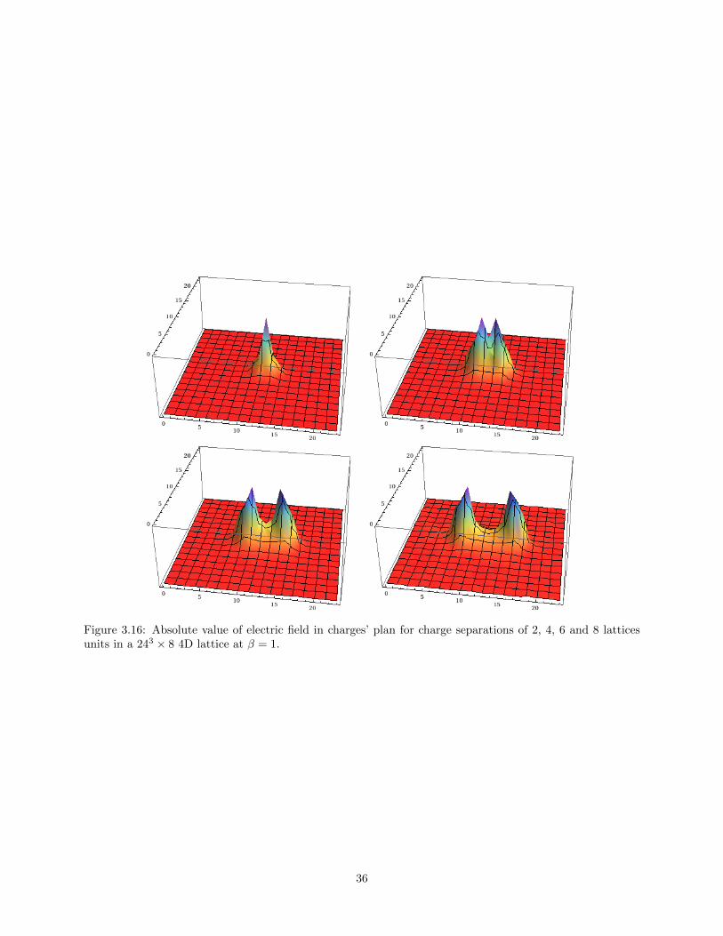
Figure 3.16: Absolute value of electric field in charges’ plan for charge separations of 2, 4, 6 and 8 latticesunits in a 243 × 8 4D lattice at β = 1.

36

0 5 10 15 20

0

5

10

15

20

0 5 10 15 20

0

5

10

15

20

0 5 10 15 20

0

5

10

15

20

0 5 10 15 20

0

5

10

15

20

Figure 3.17: Field line plot of electric field in charges’ plan for charge separations of 2, 4, 6 and 8 lattices unitsin a 243 × 4 4D lattice at β = 1. The colors correspond to a threshold to make it easier to visually separatethe stronger field caused by the charges from the small random fluctuations of the background (where redcorresponds to the stronger field).

37

Figure 3.18: Absolute value of electric field in charges’ plan for charge separations of 2, 4, 6 and 8 latticesunits in a 243 × 8 4D lattice at β = 3.

38

0 5 10 15 20

0

5

10

15

20

0 5 10 15 20

0

5

10

15

20

0 5 10 15 20

0

5

10

15

20

0 5 10 15 20

0

5

10

15

20

Figure 3.19: Field line plot of electric field in charges’ plan for charge separations of 2, 4, 6 and 8 latticesunits in a 244 4D lattice at β = 3. In red we have our result and in blue the Coulomb result.

39

Chapter 4

Conclusion

In this work we successfully implemented a gpu code to generate and study U(1) field configurations. We

applied it to the study of U(1) flux tubes in confining phase, as well as some other already well-known

quantities.

Our results for potential are in a good agreement with the predictions of the effective string model in

the confining phase, not only showing an asymptotically linear potential, but also being compatible with a

Luscher term of π/12.

In the non-confining phase the results follow the expected Coulomb 1/r potential, with the string tension

going fast to zero.

For flux tube profile we find a broadening of the flux tube according to effective string theory predictions.

However our result for σ with potential and with flux tube broadening are not compatible, it would be

interesting to verify if we can account for this discrepancy using a higher order result for the theoretical

prediction. In a study with SU(2) group in 3D (cf. [20]) going further than leading order is important

to account for the correct result at small distances. We calculated the flux tubes up to r/a = 8 that to

our knowledge is the longest distance obtained up to now without duality transformations in U(1). Also

the lattice size used in this work (244) is bigger than most of the lattice sizes used in literature in U(1)

studies (typically ≤ 164). Further research can be done, to increase the precision of the result with more

configurations and to obtain more points to the fit, possibly by calculating the r/a odd points and including

temperatures higher than 0.4 Tc.

We report a widening of the flux tube compatible with the Effective String Theory predictions, where [31]

report an almost constant width of the flux tube, although their analysis and operators used to probe field

are different. Using dually transformed lattices [37] also finds a logarithmic growth of the flux tube width

at zero temperature. It might be interesting to deepen this study in order to understand better the relation

between these results.

The usage of up-to-date numerical methods as multilevel as well as advanced computing technology as

making usage of the GPU’s processing capabilities through CUDA allows the possibility of doing this kind

of computations without having to resort on big clusters of CPU’s.

41

Appendix A

Notation and Definitions

This appendix lists some usual notation and definitions used throughout the text. It is intended to be used

as reference.

• Greek indexes (e.g. µ)

refer to directions in lattice. Direction 0 is the temporal direction, the others are space directions.

• lattice point x

refers to a specific point in lattice with coordinates given by x. It is a shortcut to a vector of 4

components xµ.

• lattice point x+ µ

refers to the next point in the lattice in µ direction.

• lattice link Uµ(x)

refers to a link that connects lattice points x and x + µ. Its value is defined in the middle point of x

and x+ µ (sometimes denoted by x+ µ2 ) and is an element of the gauge group. When specifying where

is the exact position of the link defined the following notation is used Uµ(x) ≡ eiag[Aµ(x+ µ2 )].

• U(1) phase θµ(x)

used in the context of U(1) lattice gauge theory. Refers to the phase of the link Uµ(x) so that

Uµ(x) ≡ eiθµ(x).

• plaquette Pµν(x)

smallest possible loop, built from the closed product of four links along the directions µ and ν,

Pµν(x) ≡ eiθµν(x) ≡ Uµ(x)Uν(x+ µ)U∗µ(x+ ν)U∗ν (x).

• staple Wµ(x)

sum of all the products of three links around a certain link Uµ(x)

Wµ(x) ≡∑ν 6=µ [Uν(x)Uµ(x+ ν)U∗ν (x+ µ) + U∗ν (x− ν)Uµ(x− ν)Uν(x− ν + µ)] ≡ |Wµ(x)| eiθt(x)

• Polyakov loop P (x)

product of all the links in time direction in one spatial point P (x) ≡∏Ntt=0 U0(x+ t0).

• configuration x(α)

the notation x(α) is used to denote a specific configuration. A sum on alpha∑Ncfα=1 x

(α) is used to refer

43

to a summation over all the Ncf configurations available. When several configurations are available

U(α)µ (x) may be used to specify to which configuration does the link Uµ(x) belong.

44

Bibliography

[1] J. Beringer et al. (Particle Data Group) Phys. Rev. D 86 (2012) .

[2] K. G. Wilson, “Confinement of quarks,” Phys. Rev. D 10 (Oct, 1974) 2445–2459.

http://link.aps.org/doi/10.1103/PhysRevD.10.2445.

[3] H. Hamber and G. Parisi, “Numerical Estimates of Hadronic Masses in a Pure SU(3) Gauge Theory,”

Phys.Rev.Lett. 47 (1981) 1792.

[4] J. Jersak, C. Lang, and T. Neuhaus, “Four-dimensional pure compact U(1) gauge theory on a spherical

lattice,” Phys.Rev. D54 (1996) 6909–6922, arXiv:hep-lat/9606013 [hep-lat].

[5] N. Christ, R. Friedberg, and T. Lee, “Random Lattice Field Theory: General Formulation,”

Nucl.Phys. B202 (1982) 89.

[6] M. Luscher and S. Schaefer, “Lattice QCD without topology barriers,” JHEP 1107 (2011) 036,

arXiv:1105.4749 [hep-lat].

[7] R. Gupta, “Introduction to lattice QCD: Course,” arXiv:hep-lat/9807028 [hep-lat].

[8] M. Loeve, Probability Theory. No. v. 1 in Graduate Texts in Mathematics. Springer-Verlag, 1978.

[9] R. Sommer, “A New way to set the energy scale in lattice gauge theories and its applications to the

static force and alpha-s in SU(2) Yang-Mills theory,” Nucl.Phys. B411 (1994) 839–854,

arXiv:hep-lat/9310022 [hep-lat].

[10] M. Caselle, R. Fiore, F. Gliozzi, M. Hasenbusch, and P. Provero, “String effects in the Wilson loop: A

High precision numerical test,” Nucl.Phys. B486 (1997) 245–260, arXiv:hep-lat/9609041

[hep-lat].

[11] M. Luscher, “Symmetry Breaking Aspects of the Roughening Transition in Gauge Theories,”

Nucl.Phys. B180 (1981) 317.

[12] M. Hasenbusch and K. Pinn, “Surface tension, surface stiffness, and surface width of the

three-dimensional Ising model on a cubic lattice,” Physica A192 (1993) 342–374,

arXiv:hep-lat/9209013 [hep-lat].

[13] K. J. Juge, J. Kuti, and C. Morningstar, “Fine structure of the QCD string spectrum,” Phys.Rev.Lett.

90 (2003) 161601, arXiv:hep-lat/0207004 [hep-lat].

[14] M. Luscher and P. Weisz, “Quark confinement and the bosonic string,” JHEP 0207 (2002) 049,

arXiv:hep-lat/0207003 [hep-lat].

45

[15] M. Caselle, M. Pepe, and A. Rago, “Static quark potential and effective string corrections in the

(2+1)-d SU(2) Yang-Mills theory,” JHEP 0410 (2004) 005, arXiv:hep-lat/0406008 [hep-lat].

[16] M. Panero, “A Numerical study of confinement in compact QED,” JHEP 0505 (2005) 066,

arXiv:hep-lat/0503024 [hep-lat].

[17] M. Caselle, M. Hasenbusch, and M. Panero, “High precision Monte Carlo simulations of interfaces in

the three-dimensional ising model: A Comparison with the Nambu-Goto effective string model,” JHEP

0603 (2006) 084, arXiv:hep-lat/0601023 [hep-lat].

[18] B. B. Brandt and P. Majumdar, “Spectrum of the QCD flux tube in 3d SU(2) lattice gauge theory,”

Phys.Lett. B682 (2009) 253–258, arXiv:0905.4195 [hep-lat].

[19] M. Luscher and P. Weisz, “String excitation energies in SU(N) gauge theories beyond the free-string

approximation,” JHEP 0407 (2004) 014, arXiv:hep-th/0406205 [hep-th].

[20] F. Gliozzi, M. Pepe, and U.-J. Wiese, “Linear Broadening of the Confining String in Yang-Mills

Theory at Low Temperature,” JHEP 1101 (2011) 057, arXiv:1010.1373 [hep-lat].

[21] F. Gliozzi, M. Pepe, and U.-J. Wiese, “The Width of the Color Flux Tube at 2-Loop Order,” JHEP

1011 (2010) 053, arXiv:1006.2252 [hep-lat].

[22] F. Gliozzi, M. Pepe, and U.-J. Wiese, “The Width of the Confining String in Yang-Mills Theory,”

Phys.Rev.Lett. 104 (2010) 232001, arXiv:1002.4888 [hep-lat].

[23] M. H. Quenouille, “Notes on bias in estimation,” Biometrika 43 no. 3-4, (1956) 353–360,

http://biomet.oxfordjournals.org/content/43/3-4/353.full.pdf+html.

[24] J. W. Tukey, “Bias and confidence in not-quite large samples,” The Annals of Mathematical Statistics

29 no. 2, (1958) 614.

[25] R. G. Miller, “The jackknife-a review,” Biometrika 61 no. 1, (1974) 1–15,

http://biomet.oxfordjournals.org/content/61/1/1.full.pdf+html.

[26] M. Creutz, Quarks, Gluons and Lattices. Cambridge Monographs on Mathematical Physics.

Cambridge University Press, 1985.

[27] A. Bazavov and B. A. Berg, “Program package for multicanonical simulations of U(1) lattice gauge

theory,” Comput.Phys.Commun. 180 (2009) 2339–2347, arXiv:0903.3984 [hep-lat].

[28] S. L. Adler, “Over-relaxation method for the monte carlo evaluation of the partition function for

multiquadratic actions,” Phys. Rev. D 23 (Jun, 1981) 2901–2904.

http://link.aps.org/doi/10.1103/PhysRevD.23.2901.

[29] S. L. Adler, “Metropolis overrelaxation for lattice gauge theory for general relaxation parameter ω,”

Phys. Rev. D 38 (Aug, 1988) 1349–1351. http://link.aps.org/doi/10.1103/PhysRevD.38.1349.

[30] G. Parisi, R. Petronzio, and F. Rapuano, “A Measurement of the String Tension Near the Continuum

Limit,” Phys.Lett. B128 (1983) 418.

46

[31] Y. Koma, M. Koma, and P. Majumdar, “Static potential, force, and flux tube profile in 4-D compact

U(1) lattice gauge theory with the multilevel algorithm,” Nucl.Phys. B692 (2004) 209–231,

arXiv:hep-lat/0311016 [hep-lat].

[32] M. Luscher and P. Weisz, “Locality and exponential error reduction in numerical lattice gauge theory,”

JHEP 0109 (2001) 010, arXiv:hep-lat/0108014 [hep-lat].

[33] “Nvidia specifications for nvidia geforce gtx 580 card.”

http://www.nvidia.in/object/product-geforce-gtx-580-in.html.

[34] “Nvidia specifications for nvidia tesla c2075 card.”

http://www.nvidia.com/docs/IO/43395/BD-05880-001_v02.pdf.

[35] “Nvidia reduction algorithm.” http:

//www.nvidia.com/content/cudazone/cuda_sdk/Data-Parallel_Algorithms.html#reduction.

[36] A. Amado, N. Cardoso, M. Cardoso, and P. Bicudo, “Study of compact U(1) flux tubes in 3+1

dimensions in lattice gauge theory using GPU’s,” Acta Physica Polonica B Proceedings Supplement

Vol. 5 No 4 (2012) 1129–1134, arXiv:1208.0166 [hep-lat].

[37] M. Zach, M. Faber, and P. Skala, “Investigating confinement in dually transformed U(1) lattice gauge

theory,” Phys.Rev. D57 (1998) 123–131, arXiv:hep-lat/9705019 [hep-lat].

47