fm blbs059-engle june 11, 2010 14:14 trim: 246mm x 189mm printer name ... economics and...

P1: SFK/UKS P2: SFK/UKS QC: SFK/UKS T1: SFK

fm BLBS059-Engle June 11, 2010 14:14 Trim: 246mm X 189mm Printer Name: Yet to Come



Aquaculture Economics andFinancing

Management and Analysis



Aquaculture Economics andFinancing

Management and Analysis

Carole R. EngleAquaculture/Fisheries Center

University of Arkansas at Pine Bluff

A John Wiley & Sons, Ltd., Publication



Edition first published 2010C© 2010 Carole R. Engle

Blackwell Publishing was acquired by John Wiley & Sons in February 2007. Blackwell’s publishing program has beenmerged with Wiley’s global Scientific, Technical, and Medical business to form Wiley-Blackwell.

Editorial Office2121 State Avenue, Ames, Iowa 50014–8300, USA

For details of our global editorial offices, for customer services, and for information about how to apply for permission toreuse the copyright material in this book, please see our Website at www.wiley.com/wiley-blackwell.

Authorization to photocopy items for internal or personal use, or the internal or personal use of specific clients, is granted byBlackwell Publishing, provided that the base fee is paid directly to the Copyright Clearance Center, 222 Rosewood Drive,Danvers, MA 01923. For those organizations that have been granted a photocopy license by CCC, a separate system ofpayments has been arranged. The fee code for users of the Transactional Reporting Service is ISBN-13:978–0-8138–1301-1/2010.

Designations used by companies to distinguish their products are often claimed as trademarks. All brand names and productnames used in this book are trade names, service marks, trademarks or registered trademarks of their respective owners. Thepublisher is not associated with any product or vendor mentioned in this book. This publication is designed to provideaccurate and authoritative information in regard to the subject matter covered. It is sold on the understanding that thepublisher is not engaged in rendering professional services. If professional advice or other expert assistance is required, theservices of a competent professional should be sought.

Library of Congress Cataloging-in-Publication Data

Engle, Carole Ruth, 1952–Aquaculture economics and financing : management and analysis / Carole R. Engle. – 1st ed.

p. cm.Includes bibliographical references and index.ISBN 978-0-8138-1301-1 (pbk. : alk. paper) 1. Aquaculture industry. 2. Aquaculture–Economic aspects.

3. Aquaculture–Finance. I. Title.HD9450.5.E53 2010338.3–dc22

2010013917

A catalog record for this book is available from the U.S. Library of Congress.

Set in 9.5/11.5 pt Times by Aptara R© Inc., New Delhi, IndiaPrinted in Singapore

1 2010

http://www.wiley.com/wiley-blackwell



This book is dedicated to my parents, Mildred Evelyn Orris Engle Wambold,Glenn Wambold, and Morris Engle, Jr.; my husband, Nathan Stone;

our children Reina, Eric, and Cody; andto the fish farmers of Arkansas.



Contents

Preface ix

Acknowledgments xi

I Managing Aquaculture Businesses 1

1 Starting an Aquaculture Business 3

2 Marketing Aquaculture Products 13

3 Developing a Business Plan for Aquaculture 23

4 Monitoring Economic and Financial Performance of Aquaculture Businesses 41

5 Financing an Aquaculture Business 57

6 Managing Cash Flow 67

7 Managing Capital Assets in Aquaculture Businesses 81

8 Managing Risk in Aquaculture Businesses 93

9 Managing Labor 105

II Economic and Financial Analysis of Aquaculture Businesses 115

10 The Enterprise Budget and Partial Budgeting in Aquaculture 117

11 Financial Statements: Balance Sheet and Income Statement in Aquaculture 131

12 Cash Flow Analyses in Aquaculture 143

13 Investment Analysis (Capital Budgeting) in Aquaculture 159

14 Lending in Aquaculture 173

vii



viii Contents

III Research Techniques to Analyze Farm-Level Decision-Making 183

15 Use and Misuse of Enterprise and Partial Budgets 185

16 Risk Analysis in Production Aquaculture Research 197

17 Whole-Farm Modeling of Aquaculture 207

18 Managing Government Policies and Regulation in Aquaculture Businesses 219

Bibliography 231

Webliography 235

Glossary 241

Index 255



Preface

The volume of aquaculture production worldwide hasgrown at a rate of approximately 8% per year overthe last decade. Continued growth is expected due toincreases in world population and the apparent lev-eling off of the capture of many commercial fish-eries species. Farmed salmon and shrimp productionhave grown to dominate their respective world mar-kets over the last several decades. More recently, newglobal markets have emerged for farmed species suchas tilapia (Oreochromis sp.), channel catfish (Ictaluruspunctatus) and the basa/tra species (Pangasius sp.).Continued growth, however, depends not just on de-mand but also on the economic and financial viabilityof the businesses developed.

Aquaculture production presents some unique chal-lenges for economic analysis. While there are manybooks that address the theory and methodology of eco-nomic and financial analysis, there are few that presentclear details on applications to aquaculture businesses.The few that do are quite general in nature and rely onhypothetical examples that omit the often-messy de-tails of the real world. The difficulties posed by aqua-culture businesses are rarely discussed or addressed.The problem is exacerbated by the lack of practicalknowledge and experience in aquaculture on the partof many economists. Simplifying assumptions makeanalyses more tractable, but too often obscure the prob-lems and challenges faced by those attempting to makea living from aquaculture.

As a result, researchers who wish to add an eco-nomics component to a production aquaculture trialhave little guidance. The unfortunate result is that keycosts are too often ignored, invalid assumptions aremade, and analytical tools are applied incorrectly.These errors degrade the quality of the work and maylead to erroneous or misleading conclusions.

The intent of this book is to provide a detailed andspecific set of guidelines for both aquaculture busi-nessmen and women and researchers related to the use

of economic and financial analysis of aquaculture. Thegoal of the book is to remove the mystery or “voodoo”from economic analysis as it is applied to aquacultureand to provide a guide for its accurate application.

This book discusses key issues related to bothfinancing and planning for aquaculture businesses,how to monitor and evaluate economic and financialprogress, and how to manage the capital, labor, andrisk in the business. The book works through the spe-cific application of farm management and financialanalysis tools for aquaculture. Particular attention ispaid to those line items and valuation methods thatare most often confused or in error in aquaculture. Asection on use and misuse of budgeting techniques inresearch should assist aquaculture researchers to avoidcommon mistakes. Additional chapters on risk analy-sis and whole-farm modeling provide a sense of moreadvanced techniques and their applicability. Finally,a chapter on managing government regulations pro-vides guidance for adjusting to an increased numberof regulatory activities.

The book is based entirely on aquaculture examplesand literature with an emphasis on farm-level data andanalysis. It is written in terminology that aquacultureresearchers and business persons will readily followand understand. The section on the application of eco-nomic analysis in aquaculture research is unique; noother book outlines how to value parameters measuredin aquaculture field trials.

The book includes a specific, detailed example ofa practical application in each chapter. A section onother applications in aquaculture is included to paint abroad picture of the economics of aquaculture aroundthe world while providing comprehensive guidance oneach particular topic.

The three principal audiences for this book are: (1)aquaculture business owners and managers; (2) thosewho conduct research on aquaculture production sys-tems, strategies, equipment, or management practices;

ix



x Preface

and (3) students preparing for careers either in the in-dustry or in aquaculture research. The book shouldappeal to practitioners in a number of different coun-tries, but especially those with aquaculture industries.

Aquaculture business owners and managers willlikely be most interested in Section I: Managing Aqua-culture Businesses. The chapters in this section are de-signed for those who are likely to hire an accountant todevelop the analyses, but need to know what questionsto ask and how to interpret the answers. This sectionworks through the key questions related to starting anaquaculture business, some basic marketing consider-ations, business planning, understanding how to inter-pret the financial statements prepared by accountantsfor businesses, cash flow, financing, and managementof capital assets, labor, and risk. The key focus in thissection is on the use of information to make man-agement decisions. Those aspects of aquaculture busi-nesses that are unusual or different from other typesof businesses are emphasized from the perspective ofmanaging the business effectively for profit. Chapter18 on managing government policies and regulationswill also be of interest to aquaculture business owners.

Section II, Economic and Financial Analysis ofAquaculture Businesses, is for students and thosewho wish to understand the details of how to develop

and complete the various types of economic analysesthat are commonly used in the economic analysisof aquaculture. Each chapter presents in detail themechanics and methodology for developing enterprisebudgets, partial budgets, balance sheets, income state-ments, cash flow budgets, and investment analyses.Challenges and common pitfalls associated with useof each of these methodologies are discussed in eachchapter.

Section III, Research Techniques to Analyze Farm-Level Decision-Making, is written especially for thosewho conduct research on aquaculture production sys-tems, strategies, equipment, or management prac-tices. Misleading assumptions, omitted costs, over-estimating revenues, and misapplication of researchdata can be common in economic analysis based onaquaculture research. This section reviews these chal-lenges and describes detailed approaches to developingaccurate economic analyses with production researchdata.

The book includes an annotated bibliography and awebliography of resources. Software products avail-able for economic and financial analyses are listed anddescribed. It is my hope that you will find this bookuseful and that it will help aquaculture businesses tobe efficient, viable, and profitable.



Acknowledgments

There are many people who contributed either directlyor indirectly to the content of this book. Some of thismaterial was drawn from earlier training programsdeveloped with the assistance of Diego Valderrama,Steeve Pomerleau, and Ivano Neira. Ganesh Kumarhas provided invaluable assistance throughout. In-sightful and useful review comments were provided

by Diego Valderrama, Anita Kelly, Madan Dey, andGeorge Selden. Umesh Bastola, Pratikshya Sapkota,and Abed Rabbani also provided suggestions. Finally,fish farmers throughout Arkansas and other statesprovided the continuous ground truthing of theeconomics and financing of aquaculture.

xi

P1: SFK/UKS P2: SFK

c01 BLBS059-Engle June 11, 2010 9:22 Trim: 246mm X 189mm Printer Name: Yet to Come

Section IManaging Aquaculture Businesses

INTRODUCTION TO SECTION I:MANAGING AQUACULTUREBUSINESSES

This section focuses on the use and application of eco-nomic tools and interpretation of their results. It isdesigned primarily for owners and managers who hireothers to prepare financial statements and analyses. Atthe same time, those who are trained to conduct eco-nomic and financial analysis but who are not familiarwith aquaculture should also find this section useful.

Aquaculture is a management-intensive business.The need for intensive and skilled management stemsfrom the high level of capital invested in the facil-ities, and in the high levels of operating capital re-quired to operate a competitive and profitable business.Throughout aquaculture, undercapitalization (not hav-ing enough capital to make payments and survive the

sometimes lengthy startup periods) has been a consis-tent problem.

Individual companies must answer a series of ques-tions that involve pricing, output, and market posi-tioning. Key questions that the manager must answerinclude: (1) how much should be produced; (2) howmuch input should be used; (3) what is the optimalsize of the business; (4) how should cash flow be man-aged; (5) how should risk be managed; (6) how will thebusiness be financed; and (7) how can business perfor-mance be optimized? Thus, it is the manager who mustdevelop the business plan, monitor economic and fi-nancial performance of the business, and manage cash,capital, labor, and risk. Each of the following chaptersdiscuss specific aspects of the types of managementfunctions and decisions that need to be made by themanager.

P1: SFK/UKS P2: SFK


P1: SFK/UKS P2: SFK


1Starting an Aquaculture Business

Aquaculture has grown rapidly in volume and in com-plexity around the world in the last several decades.While aquaculture has a centuries-long history as asource of food for households in Asia and Africa, themost dramatic change in more recent years has beenthe development of aquaculture businesses into com-plex industries. These industries operate on nationaland international levels.

Development of efficient and viable businesses re-quires careful evaluation and thorough planning for thenew business. This book presents details on the pro-cess of business planning (see Chapter 3) as well ason how to prepare the various types of financial state-ments needed for thorough planning (see Chapters 10through 14). Chapter 1 begins by outlining steps to beconsidered before starting the business.

The new business owner must think carefully aboutwhat will set his or her business apart, both from otherexisting businesses and from other future businesses. Itis critical to identify the strengths, abilities, and skillsowned and available that will help the farm owner tobe successful. This chapter discusses the motivationand goals for starting an aquaculture business, andthe capital- and management-intensive nature of aqua-culture. Marketing challenges and trade-offs associ-ated with various organizational structures, financing,and the availability of resources are contrasted. It con-cludes with a discussion of permits, regulations, andsources of assistance. Figure 1.1 illustrates the varioussteps that will be needed to start a successful aquacul-ture business.

MOTIVATION AND GOALS

The first step to starting an aquaculture business is tocarefully consider one’s goals and motivation. An in-

dividual interested in starting an aquaculture businessmust fully understand why he or she wants to do this.Some individuals enjoy working outdoors with fish anddislike office work and paperwork. These individualsmay do an admirable job like raising fish on the farm.However, inadequate attention to the business aspectsof the aquaculture business will result in financial fail-ure. If the owner spends all his or her time caring forthe fish, who will take care of the permits, regulations,financial statements, and economic performance of thebusiness?

Others who wish to start an aquaculture businessmay view it as a way to make a great deal of money.There certainly are success stories of aquaculture busi-nesses that have become profitable businesses. How-ever, aquaculture businesses are intensive businessesthat require management committed to working longhours under often difficult conditions. Who will pro-vide that level of management?

Still others view aquaculture as the wave of the fu-ture and want to get in on the ground floor. However,businesses developed to raise the latest “hot” specieswith the newest production technology frequently arebeset with substantial levels of financial, price, andyield risk. Aquaculture entrepreneurs must be preparedto manage the degree of risk associated with their busi-ness model and plan.

It is important to develop clear and specific goals forthe business from the beginning. For example, what isadequate revenue for one individual may not be suf-ficient to entice another to invest the necessary timeand money. The effects of starting a new business onthe farmer’s family must be considered carefully. Willfamily members be supportive and helpful or will theyresent the time that must be invested in the business?The early years of an aquaculture business may gener-ate minimal revenue, and the family may be requiredto live for a time on reduced income.Aquaculture Economics and Financing: Management and

Analysis, Carole R. Engle, C© 2010 Carole R. Engle.

3

P1: SFK/UKS P2: SFK


4 Managing Aquaculture Businesses

Assess available resources, strengths, and weaknessesSelect production system and species to raise

Find

Markets

Financing

Management

Develop a detailed business plan:

• Marketing plan• Organizational and management plan• Labor plan• Financial plan

Acquire permitsDevelop support network

Construct facilitiesInitiate production

Figure 1.1. Starting an aquaculture business.

AQUACULTURE IS ACAPITAL-INTENSIVE BUSINESS

The majority of aquaculture businesses require sub-stantial amounts of both operating and investmentcapital. One of the largest problems encountered instarting an aquaculture business often is to acquire suf-ficient capital. Undercapitalized farms and processingplants rarely survive. Careful thought and planningneed to go into determining the amount of capitalneeded to operate at an efficient level and to identi-fying sources for the needed capital.

Capital requirements begin with the investment cap-ital needed to purchase land, build production facili-ties, and purchase equipment. Depending on the spe-cific location, new roads may need to be constructed,electric power lines may need to be installed, or theremay be additional infrastructure required that will in-crease the total amount of investment capital needed.Capital required for marketing facilities must be in-cluded in the planning. Is a shed needed to hold, grade,and sell the fish? If so, a water supply system to fillhauling trucks will also be required. Perhaps an icemachine is required, depending on the form of theproducts sold. If the farm will do its own hauling and

transportation, then the trucks, tanks, oxygen systems,and loading equipment will also be needed. In all, in-vestment capital for an aquaculture business typicallywill be several thousand dollars an acre of produc-tion for pond systems, and can range from $0.30 to$7.00/lb across the many different types of speciesand production systems. More information on invest-ment capital requirements can be found in Chapter 10,and techniques to measure the profitability of such aninvestment can be found in Chapter 13.

The high level of investment capital required for anaquaculture business results in high levels of annualfixed costs (see Chapter 10 for more details on whatconstitute annual fixed costs). The best way to reducethe fixed cost portion of the cost of producing fishis to produce at an intensive level with high yields.High yields spread the annual fixed costs over a greaterlevel of production and lower the cost per pound ofproduction.

Operating capital requirements often are as substan-tial as investment capital requirements for aquaculturebusinesses. Frequently, this is because high yields areneeded to lower the per-pound annual fixed costs andkeep production costs at a competitive level. Achievinghigh yields requires high numbers of fingerlings, largeamounts of feed, greater electricity for aeration, andcorresponding amounts of other inputs such as labor,repairs and maintenance, and fuel. Operating costs fre-quently can be $2,000–$5,000/acre for pond systemsand $33,000–$150,000/acre for intensive systems suchas raceways and indoor systems.

Operating cost requirements are compounded by thefact that some types of fish raised do not reach marketsize in one growing season. Thus, the prospective fishfarmer often must prepare to operate the business formore than a year without receiving revenue from thebusiness. Careful financial planning and good commu-nication with one’s banker are keys to having accessto sufficient amounts of capital with which to build thebusiness until it reaches its full production capacity.

The high levels of capital required for many aquacul-ture businesses result in substantial amounts of finan-cial risk (see Chapters 8 and 16). The profit potential isoften accompanied by a variety of risks, and the largesums of money invested in an aquaculture businesscan be lost quickly. The best method to prevent suchlosses is adequate and thorough planning, monitoring,and assessment of the economics and finances of theaquaculture business throughout its life. If the owner isnot willing to spend the time to monitor the business’financial performance, then it is essential to hire or

P1: SFK/UKS P2: SFK


Starting an Aquaculture Business 5

retain an expert to keep a constant and close eye on itseconomic aspects. Otherwise, the likelihood of failureand severe financial losses is high.

AQUACULTURE IS AMANAGEMENT-INTENSIVEBUSINESS

The high levels of investment and operating capital re-quired in aquaculture businesses, along with the inten-sive nature of production of aquatic animals requiresa high degree of management. When aquatic animalsare confined in a production unit, constant attentionis needed to the quality of the growing conditions forthe fish. Maintaining adequate levels of oxygen andother critical water quality parameters, and prevent-ing problems associated with the breakdown of wasteproducts in the system, takes careful and constantmonitoring. Diseases spread rapidly when animals aremaintained in close confinement. Thus, attention mustbe paid to monitoring the health of the animals andtaking necessary actions when there are indications ofdisease.

Marketing and sales of aquatic products can repre-sent management challenges depending upon the na-ture of the target market. Farms engaged in direct saleswill require a great deal of management attention tomarketing functions and activities. Even farms thatsell directly to a processing plant must have managerswho pay close attention to the requirements of pro-cessors. These requirements include quality standardsand delivery requirements, among others, to minimizedockages from fish that do not meet specifications.Top managers ensure that their farm is considered tobe a preferred supplier, one that consistently deliversquality fish, within specification, and on time.

Management must keep a close eye on costs andproduction efficiencies throughout the production pro-cess. This includes monitoring the efficiency of labor,feed usage, use of electricity and fuel, and use andcare of equipment. Feed, for example, is frequentlythe largest single component of the cost of raising anaquaculture crop. Feeding carefully and appropriatelywill ensure a better feed conversion ratio and will re-sult in more pounds of fish produced per pound offeed applied. Similarly, judicious use of aeration canprovide adequate oxygen levels by turning aerators onsequentially, as needed, rather than turning on moreaerators than are needed at one time. Taking time tokeep equipment well maintained and to ensure that itis operated correctly will reduce the costs of repairs

and will extend its life. This will reduce the cost ofequipment as a percentage of the total cost of produc-tion.

Moreover, the manager must be able to think andplan strategically. Preparing to stay ahead of fu-ture challenges requires examination of the business’sstrategic plan from a variety of different perspectives.

MARKETING CHALLENGES

Many individuals who wish to start an aquaculturebusiness are captivated by the animals and plants thatthey wish to raise and will spend many hours talkingabout their biology and growing requirements. How-ever, the marketing challenges of starting a new aqua-culture business often are greater than the productionchallenges and ultimately more important. Successfulaquaculture businesses are managed and owned by in-dividuals who spend as much time exploring marketingoptions and trends as they do working on productionefficiencies. Chapter 2 of this book discusses market-ing issues and strategies related to aquaculture prod-ucts in greater detail and Chapter 3 outlines steps inthe development of marketing plans as part of an over-all business plan. This chapter discusses some generalconcepts.

There are a number of overarching trends and chal-lenges that prospective aquaculture business ownersshould consider. Most species that are being aquacul-tured at one time were primarily a wild-caught species.Many of these species have existing markets and de-mand that were based originally on supply from cap-ture fisheries. Preferences for wild-caught as comparedto farmed fish vary by region. Care must be taken to un-derstand these preferences in the market targeted forthe business’s product. As farmed product becomesavailable in the market, it frequently must competewith wild-caught product that is already well estab-lished in the market. However, the cost of producingfarmed fish, especially in the early years of startupbusinesses, requires a price that often is higher thanthat of wild-caught fish. To establish a new product inthe market often requires differentiating it from wild-caught and other similar products to capture a pricethat will cover production costs.

The seafood market has undergone dramaticchanges in the last several decades. The possible ef-fects of current and emerging trends must be consid-ered carefully in planning for successful marketingprograms. Seafood in earlier decades was primarilya locally sourced, fresh product supplied by either

P1: SFK/UKS P2: SFK



fishermen or specialized jobbers and small-scalewholesalers. Changes in packaging and freezing tech-nologies have opened the door for global trade inseafood that has continued to increase dramatically.The increase in global trade in seafood has resultedin a number of conflicts and competition with fishraised domestically. All types of fish and seafoodare now shipped around the world to satisfy variousmarkets.

Dynamic markets like those for seafood, while chal-lenging, can also offer opportunities for entrepreneurs.For example, the shrimp and salmon industries world-wide have benefited from the increase in global tradeand technology. These segments of aquaculture havegrown to dominate shrimp and salmon markets world-wide.

Food marketing in general has undergone dramaticchanges in recent decades that have resulted in changesalong the supply chain. The driving force has beenthe emergence of strong market power at the levelof the large hypermarket discount retail sector, exem-plified by companies like Wal-Mart. In response tothis concentration of market power, wholesalers andfood service distributors have also become more con-centrated. This has increased pressure on growers toeither consolidate by integrating vertically to capturemarket power, or to form cooperative or other formsof organizations to be able to compete.

Startup aquaculture businesses must identify thespecific market that the business plans to target. Theoverall marketing plan (see also Chapter 3) must alsoidentify the competition and the unique position thecompany’s product will occupy in the market. Theproduct must be defined well and must match the wayit is positioned in the market for the targeted customers.Careful attention should be paid to the size of the mar-ket, long-term price trends, and distribution patternsof similar products.

The marketing plan must lay out an effective pro-motion and advertising plan. Even the smallest-scaleaquaculture farms must have a plan to spread the wordabout their products. Promotion is a way to transmit in-formation about the attributes of the product, the price,and why the consumer should purchase it.

Appropriate and effective market channels must bedeveloped. Is the farmer planning to transport all thefish produced to the various markets? The amount oftime needed to transport fish to markets must be deter-mined and adequate personnel included in the businessplan. The length of round trips that can be undertakenfeasibly can be an important factor. If the farmer doesnot intend to transport his or her own fish, relationships

and agreements will be needed with a wholesaler ordistributor.

ORGANIZATIONAL STRUCTUREFOR THE AQUACULTURE BUSINESS

Most farms in the United States have a single ownerand are classified as sole proprietorships. In a soleproprietorship, the farmer is self-employed and haslegal title to the property. This is the simplest form ofbusiness structure, but it also entails the greatest risk.Risk results from the liability for any debt obligationsor accidents that falls entirely on the owner in a singleproprietorship. Moreover, the liability is not limitedto what the farmer has invested in the business. Thefarmer can lose his or her land and home as a result ofsevere adverse situations.

Some farmers form partnerships with family mem-bers or others to gain access to additional resourcessuch as land, equipment, labor, or management. Part-nerships can be either general or limited. Partners sharein all ownership, management, and liability in a generalpartnership. Limited partners share in the profits andlosses of the business but not in the management. Inthis way, the limited partner provides resources suchas capital, but management decisions are under thecontrol of the principal owner.

Some segments of aquaculture have integrated verti-cally and have developed into corporations. In a corpo-ration, capital is provided by shares of stock, and themanagement and control are provided by the stock-holders, the board of directors, and the officers. Theboard sets policies, and the officers manage the dailyactivities of the company. Stockholders, while ownersof the company, are not personally liable for actionsof the corporation. Their liability is limited to theirinvestment in stocks.

There are also subchapter C and subchapter S cor-porations. With C corporations, dividends received bystockholders are taxed as income, while S corporationsare taxed as limited partnerships. The officers are paidbefore the remaining profits are distributed.

AVAILABLE RESOURCES

An important step in starting an aquaculture businessis to develop a frank assessment of the resources avail-able for the business. New businesses fail more oftenthan they succeed, often due to the lack of adequateresources. The assessment of available resources be-gins with the individual. The owner must be inno-vative, persistent, resourceful, and determined to find

P1: SFK/UKS P2: SFK



solutions to the many problems that will arise. Theassessment should extend to physical resources avail-able that include land, existing ponds, wells or othertypes of water supply, farm equipment, and buildings.The assessment must be thorough and detailed. Forexample, the individual may have an adequate quan-tity of land available, but current or impending zoningregulations may prohibit its use for aquaculture. Waterand soil analyses should be done to check the suitabil-ity for the species to be considered. Some freshwatershave enough salinity to consider some crops like ma-rine shrimp that can tolerate low levels of salinity.There must also be adequate backup equipment in theevent of breakdowns, generators for power outages andbackup aeration equipment. Resources also include theavailability of adequate quantities of seedstock.

The availability of labor resources can be an impor-tant factor in the success or failure of a new business.The assessment of labor availability should include anyfamily labor that is available to assist with the farm.A realistic assessment must be made of the local laborsupply and the availability of adequately trained la-bor that can be hired for the aquaculture business. Thetype of labor is also an important consideration. Aqua-culture businesses often require more skill than someother types of agriculture, and the ability of workersto handle the new responsibilities must be evaluatedcarefully. For example, workers who cannot swim orwho are afraid of the water may have difficulty adjust-ing to working around it constantly. Much aquaculturerequires long and irregular hours during the maingrowing season. Workers may or may not be willing towork such hours. The degree of equipment on the farmrequires a great deal of maintenance. An aquaculturebusiness requires either a mechanic hired on the farmor the business must be prepared to have higher repairand maintenance costs.

The availability of management resources must beassessed. The level of expertise and skill of the ownerto manage the production, marketing, and financingof the aquaculture business must be evaluated frankly.If the owner has excellent aquaculture skills but isweak in financial analysis, an appropriate accountantor financial analyst will need to be hired, contracted,or retained. Similarly, if the owner has good businessskills in marketing and financing, but lacks experiencein culturing aquatic animals, hiring a production man-ager with adequate aquaculture skill and expertise willbe essential.

Sufficient capital resources must be available aswell. Both investment and operating capital are re-quired in necessary quantities to be received at ap-

propriate times. The operating line of credit must bestructured to continue the business throughout the en-tire startup period during which the business beginsto generate returns. Depending on the type of busi-ness, this may be a period of 2–3 years before sub-stantial revenue can be generated from the aquaculturebusiness. The investment capital must be available insufficient quantities to provide facilities to minimizerisk. This includes sufficient redundancy in equipmentto cover power outages, breakdowns, and unantici-pated extended periods of adverse weather conditions.Maintenance requirements must be accounted for infinancial planning. This includes the capital to be ableto replace all equipment and facilities when necessary.

The availability of adequate credit will depend inpart on the ability of the owner to finance the opera-tion through equity or to have the credit capacity toborrow the necessary amounts of capital. This in turnwill depend upon the individual’s balance sheet, avail-ability of collateral, and overall credit worthiness.

The particular species selected and their productforms are critical decisions. These must match theprojected price point and the quantity demanded forthat product form for that species. In selecting thespecies to be raised, thought must be given to whetherthere is competition from imported species or capturefisheries, or both. Diversifying farm production withseveral species also serves to spread the market risk ofprice downturns for one specific species.

The key to starting a successful aquaculture busi-ness is to match the species to be produced, the pro-duction system to be used, and the scale and scopeof operation with the available markets and resources(labor, land, capital, and management). Mismatchesare likely to result in business failure. For example, aparticular species and production system may exhibitstrong economies of scale. If the owner is unlikely tobe able to acquire sufficient capital to construct andoperate a farm of a large size, it is better to rethink thebusiness plan to develop one that is workable with thecapital resources available. Undercapitalization is of-ten a major reason for failure of aquaculture farms andprocessing plants. Mismatches between projected andactual capital requirements result in financial failure.

FINANCING

Adequate financial resources are essential to a suc-cessful business, and the ability to acquire sufficientcapital is a key factor. One of the first steps is to identifythe sources of capital that are available. Venture cap-ital can be difficult for aquaculture and often follows

P1: SFK/UKS P2: SFK



certain patterns and trends that may not always favorfinancing aquaculture businesses. Private capital frompartners, whether active or silent, can be considered inestablishing the business. However, private lenders fi-nance most aquaculture businesses. Many lenders maybe skeptical about aquaculture and view it as a riskybusiness. Perceptions of high risk in aquaculture maylead to less favorable terms of lending, requirementsfor greater owner equity in the business, higher inter-est rates, or refusal to consider loans for aquacultureventures.

Financing from private lenders can also be com-plicated by the fact that many lenders may not havesubstantial experience with aquaculture. Lack of fa-miliarity with the business can result in unwillingnessto assess business loan proposals; the loan officer maynot be comfortable with the estimates of yields, costs,or efficiency measures that form the basis of the pro-posal. It may be necessary to spend a great deal oftime working with a lender to help them understandthe basics of aquaculture, introduce them to peoplewho are knowledgeable about successful aquaculturebusinesses and the keys to their success, and to keepthem informed of the most recent trends in aquacul-ture. It is important to plan for adequate capital toprovide for the family through the very difficult earlyyears of the business.

HARVESTING AND PROCESSING

Decisions must be made early on in the developmentof an aquaculture business on how the fish or otheranimals will be harvested and whether they will beprocessed, stored, and transported by the farm busi-ness. If not, these services will need to be contracted.Serious thought needs to be given to the implicationsof these decisions. In areas with little aquaculture pro-duction, these services may not be available. If thefarm owner must hire a seining crew, process the prod-uct, and store and transport it, the owner likely willneed to operate on a relatively large scale. There aresome examples of small-scale aquaculture businessesthat perform these functions, but typically these willrequire a larger scale of business. Processing in par-ticular has substantial economies of scale that must beconsidered before proposing this type of componentto the business.

Product handling throughout transportation and pro-cessing will affect the end quality of the product. Ifproper conditions are not maintained during harvestand transport, the quality of the fillet may suffer. Sim-

ilarly, if processed fillets are not stored or packagedproperly, the result will be a poor quality product. Ad-equate planning for these functions is necessary.

PERMITS AND REGULATIONS

Part of a careful assessment for a startup business in-cludes identifying the permits and regulations that willaffect the new business both currently and in the fu-ture. Chapter 18 discusses the role of regulations andpreparing to manage them in greater detail.

There are a wide variety of types of permits that arerequired in different states, provinces, and countries.These permits may refer to the site, the business, ac-cess to water supplies, discharges, predator control, orprocessing.

All legal and regulatory statutes relevant to the busi-ness must be understood and planned for. Some typesof permits may require lengthy application periods thatmay delay startup of the business.

SOURCES OF HELP

There are a number of sources of help and techni-cal assistance available to the individual consideringa startup aquaculture business. Table 1.1 summarizesseveral types of assistance available. It is advisable todevelop an excellent relationship with these groups.Universities, extension agents, trade associations, anddiagnostic laboratories are all essential sources of sup-port, technical assistance, and help. Joining the rele-vant trade association and inclusion on the mailing listof the local extension office will ensure that the newfarmer receives the latest updates on permits, regula-tions, issues, and research.

Plans must include developing contacts with the lo-cal diagnostic laboratories, pathologists, and techni-cians. Understanding the best way to submit samplesfor diagnosis and training workers in the proceduresrequired will reduce the time to initiate appropriatetreatments.

International sources of help include internationalnetworks that promote aquaculture such as the Net-work of Aquaculture Centres in Asia-Pacific (NACA).A network in Eastern Europe, the Network of Aqua-culture Centres of Central-Eastern Europe (NACEE),similarly promotes aquaculture and provides informa-tion to industry.

In the United States, available help includes per-sonnel of United States Department of Agriculture-

P1: SFK/UKS P2: SFK



Table 1.1. Sources of Help and Assistance for New Aquaculture Businesses.

Type of organization Type of assistance

Extension services Research-based informationDisease and water quality diagnostics laboratories Diagnosis of disease and water quality problemsIndustry trade associations Updates on issues

State Political actionNational Trade journalsInternational NewsSpecies specific Updates on issues, meetingsMultispecies Updates on issues, meetings

Government agencies Information on permits and programsState Information on permits and programsFederal Information on permits and programs

Related industry segments Information on trends, costs, productsEquipment suppliers Information on trends, costs, equipmentFeed manufacturers Information on trends, costs, productsSupply company representatives Information on trends, costs, products, permitsBank Information on financial position and trends

Local government entities Information on trends and permitsChambers of commerce News and local eventsEconomic development offices Business and financial assistance and new programs

Animal Plant and Health Inspection Service/WildlifeServices. Permits are required in the United States tocontrol fish-eating birds. Severe fines and penaltiescan be levied on farmers who have not obtained thenecessary permits. Wildlife Services personnel have avariety of programs to provide assistance in the controlof fish-eating birds and in the process of obtaining thenecessary permits.

Local and state aquaculture associations can be ofgreat help. Subscriptions to aquaculture journals, mag-azines, and newsletters help to keep abreast of currentnews and impending legislation.

Extension professionals are some of the best sourcesof information. These are trained scientists who areskilled in techniques to disseminate information effec-tively. They also have the latest research results at theirfingertips and may offer opportunities for farmers tocooperate in on-farm or verification trials.

Some states and provinces have government officesthat will assist aquaculture growers. Equipment sup-pliers, feed manufacturers, supply company represen-tatives, and restaurant owners can be good sources ofinformation on trends, costs, and market data. Localchambers of commerce, economic development of-fices, and banks can also provide relevant and usefulinformation.

RECORD-KEEPING FORAQUACULTURE BUSINESSES

The intensive nature of successful businesses requiresmanagers to maintain detailed records. Those contem-plating starting an aquaculture business should prepareto spend time to maintain records and to analyze themperiodically throughout the year. This level of man-agement can make the difference between success andfailure.

Records required will include complete records oninput purchases, use, and inventory. Labor and salesrecords that indicate the quantity sold, the price re-ceived, and any dockages incurred with each sale mustbe maintained. The ability to sort records into feedamounts and fish sales by pond or other fish cultureunit will provide the manager with a means to evaluatepond-level performance and relate this back to man-agement changes in that pond. Reports from diagnosticlaboratories on disease incidence by pond will enablethe manager to search for ways to minimize lossesdue to disease. Financial records must be maintainedfor each loan along with depreciation schedules forall equipment in the business. All paperwork relatedto permits and compliance with regulations must bemaintained over time along with all chemical use onthe farm.

P1: SFK/UKS P2: SFK



Each of the following chapters presents detailedsuggestions on how to organize and use records tomonitor and evaluate farm performance relevant to thetopic discussed in each chapter. Management decisionsmade from detailed farm records will be more effec-tive and have greater positive results over time if basedon detailed historical performance records of the farmbusiness.

PRACTICAL APPLICATION

Throughout this book, each chapter includes an exam-ple of an application of the material presented in eachchapter to the case of a fish farm. To start such a farm,the owner will need to begin to address the criticalissues related to acquiring the necessary managementskills and capital. If the owner is not skilled and expe-rienced in managing a fish farm, it will be necessary torecruit and hire a skilled manager. Careful thought asto how to obtain the capital that will be needed mustbe given from the very beginning. Preliminary contactswith lenders will be necessary to identify those morelikely to loan to fish farmers and to identify the levelsof lending that each bank can provide.

Decisions related to the overall structure of the busi-ness can affect the supply of capital available forthe fish farm. Developing a partnership or joint ven-ture with a friend or family member can provide asource of capital. The overall financial plan needsto detail the capital that will be available from theowner and any partners and how much will need to beborrowed.

Marketing decisions also will need to be made earlyon in the planning process for the business. Overviewsof the market for that particular business and analysisof its position in the market can be important. Therest of this book provides details of each componentand analysis that is required to start and maintain asuccessful aquaculture business.

OTHER APPLICATIONS INAQUACULTURE

Engle and Valderrama (2001) developed a trainingmanual designed to assist shrimp growers to beginto develop business plans. The Engle and Valder-rama (2001) document emphasizes the financial state-ments needed for a comprehensive business plan forshrimp farming in Honduras. A CD is provided withspreadsheet templates to assist those who wish to de-

velop comprehensive business plans for their shrimpoperations. Self-guided tutorials and exercises areincluded.

SUMMARY

Aquaculture businesses should be entered into only af-ter considerable thought and analysis. Greater capital,more intensive labor, and high levels of managementare required to be successful in aquaculture regardlesswhether the business is large or small.

Comprehensive business and marketing planningis necessary. However, other considerations such aseffects on the family, personal motivations, and theavailability of adequate resources must also be ana-lyzed carefully. The remaining chapters in this bookpresent detailed information on the steps needed bothto start up and to maintain a successful aquaculturebusiness.

REVIEW QUESTIONS

1. What types of specific goals must be set whenstarting an aquaculture business?

2. Why is it important to assess one’s motivation toenter into an aquaculture business?

3. Why is aquaculture considered to be a capital-intensive business? Identify some specific exam-ples of the capital requirements for various aqua-culture businesses.

4. Where does financial risk come from?

5. Why is aquaculture considered to be amanagement-intensive business? Give some spe-cific examples for various types of aquacultureproduction.

6. What are some of the marketing challenges in-volved in starting up aquaculture business? Givesome specific examples.

7. What types of resources must be available for dif-ferent types of aquaculture businesses? Pick twodifferent aquaculture production systems and con-trast the differences in resource availability thatwould be required.

P1: SFK/UKS P2: SFK



8. List three types of organizational structures thatcan be used for aquaculture businesses and com-pare the advantages and disadvantages.

9. What are some of the key considerations relatedto financing new aquaculture businesses?

10. What are some sources of help and assistance fornew aquaculture businesses?

REFERENCE

Engle, Carole R. and Diego Valderrama. 2001. Eco-nomics and management of shrimp farms trainingmanual. In: M.C. Haws and C.E. Boyd (eds). Meth-ods for Improving Shrimp Culture in Central Amer-ica. Managua, Nicaragua: Editorial-imprenta, Uni-versidad Centroamericana. pp. 231–261. ( in Englishand Spanish)

P1: SFK/UKS P2: SFK


P1: SFK/UKS P2: SFK


2Marketing Aquaculture Products

The focus of this book is on the economics and financeof aquaculture businesses. However, an aquaculturebusiness will not be successful without a marketingprogram and plan that is appropriate and workablefor that particular business. This chapter summarizescritical factors involved in identifying and developingmarkets for aquaculture products. For a completediscussion and presentation of marketing aquacultureproducts, readers are referred to Engle and Quagrainie(2006).

THE ESSENCE OF SUCCESSFULMARKETING

The first essential point to understand about market-ing is that marketing is not synonymous with “sales.”A salesman may or may not be a marketer. Success-ful marketing results in sales, but product sales donot always mean that there is a successful market-ing program in place. Aquaculture businesses will notsucceed without a successful marketing program intoday’s food market.

Successful marketing involves development of acomplete plan that is cohesive and meshes seamlesslywith a number of factors. A successful business mustidentify which specific set of customers the businessis seeking to attract and what that group of customerswants to buy. Moreover, the business must find a wayto meet those customers’ wants and needs better thanany other business. The price charged needs to matchthe customers’ expectations in such a way that theybelieve they receive enough value to justify what theypay for the product. This type of price/quality positionfor the product must be at a price point that resultsin a profit for the business. The business’ promotionalstrategy must effectively communicate how the prod-

uct uniquely meets the preferences of the targeted con-sumer groups. Lastly, the aquaculture business mustidentify the most convenient locations for the exchangeof product to occur for their targeted consumer group.These factors must all mesh and function together as asingle company concept to be successful.

The Importance of DemandCharacteristics

Quantitatively measured characteristics of consumerdemand can shed some light on how some of thesefactors interact. Economists measure demand quanti-tatively by regressing the price of a product againstindependent variables that often include the quantitysold of the product, incomes, and tastes and prefer-ences, among others. Economists then use the esti-mated demand relationships to calculate elasticity, theproportional change in quantity demanded in responseto a change in price. Elasticity is important to a discus-sion of markets because, if demand is elastic, an in-crease in price will result in a relatively larger decreasein the quantity demanded, such that total revenue tothe producer will go down. However, with inelasticdemand, the price increase may still result in a lowerquantity demanded, but the quantity response is pro-portionately less than the change in price. When thisoccurs, the total revenue to the grower will increaseas prices increase. Development of specialty marketstypically depends upon inelastic demand to success-fully command the higher prices common in specialtymarkets.

One characteristic of products with inelastic demandis that there are few close substitutes for the prod-uct. After all, if all shrimp sold (imported, domestic,farmed, wild-caught) are identical, why would a buyerpay a higher price for one particular farm’s shrimp?Thus, one key to developing a product for a specialtymarket is to differentiate it from the competition.

Aquaculture Economics and Financing: Management andAnalysis, Carole R. Engle, C© 2010 Carole R. Engle.

13

P1: SFK/UKS P2: SFK


14 Managing Aquaculture Business

Product Differentiation andPositioning

Efforts to develop a differentiated product must care-fully consider where the product needs to be positionedin the marketplace. This decision must consider thecosts of production, the competition, consumer per-ceptions of the product, and closely competing prod-ucts. A product-space map (Figure 2.1) can be usedto help make this decision. Products can be positionedas a high-quality and high-priced product or, at theother end of the spectrum, a low-quality and low-pricedproduct. The key is to match consumers’ expectationswith the price. Certain market segments are willing andable to pay high prices for a product that is expectedto be of high quality.

Product positioning reflects the combination of thespecies, product form, packaging, and its price. Anyattribute that adds value, such as a spice package, mari-nade, or the package size, may affect the way a productcan be positioned and how it can be differentiated fromother products.

Aquaculture growers, particularly smaller-scalegrowers, often prefer to target specialty markets be-cause prices frequently are higher. Specialty marketingis a choice to produce a high-quality product to capturea high price. To be successful, the marketer must havea clear understanding of which attributes will entice aconsumer to pay a higher price. Equally important is

Low quality

Lo

w p

rice

High quality

Hig

h p

rice

Lobster

Trout

Jumboshrimp

Freshwaterprawns

Tilapia

Atlanticsalmon

Mackerel

Carp

Bullhead

Frozen crab legs

Refrozenshrimp in grocery

stores

Jumbo shrimp held past shelf life

Figure 2.1. Generalized example of a product-space map with various types of seafood species. The exact positionof a product will reflect not only the species, but product form, size, and handling.

how the specific product embodies those attributes to agreater extent than the competition. Why should some-one pay more for your product? What is it specificallythat uniquely presents the value that the consumer issearching for? Products must be positioned to be dif-ferentiated from other products in such a way that thevalue of the product is worth what the consumer mustpay for it.

Successful products attract competition over time.Other companies will learn to produce similar productsand perhaps extend the product concept and line. Whenthis happens, the product will no longer be unique. Thebusiness needs to be prepared for competition that willcome if the new products are successful. Each productthat becomes established in the market goes through atype of life cycle (Figure 2.2). In the early stages fol-lowing the introduction of product, sales grow rapidlyas customers become aware of the product and begin toexperiment with it. However, at some point, the prod-uct reaches a stage of maturity when it attracts com-petition. The rate of growth of product sales begins toslow as the sales volume reaches a maximum. Productsales then begin to decline. Companies with productsin the maturity stage must begin to either search outnew markets (either new geographic markets or newmarket segments) or begin to develop new products.

The price point of the product as the business haspositioned it in the market must be adequate to covernot just production costs, but marketing costs as well.

P1: SFK/UKS P2: SFK


Marketing Aquaculture Products 15

Growth Maturity Decline

Introduction

Time

Fin

anci

al p

erfo

rman

ce

Sales revenue

Figure 2.2. A theoretical diagram of a product life cycle indicating its various stages.

A high price is meaningless if total costs of productionand marketing are higher still. The business will not beprofitable. If the business plan requires the producerto carry out all marketing functions and activities,these costs must be included in the financial analysesof the plan. Marketing costs can be considerable andcan frequently include the costs of hauling live fishor transporting processed fish, off-flavor checking,marketing equipment such as baskets, dip nets, andoxygen systems, supplies like ice and bags, andcommunication systems that include telephone, fax,and Internet charges. Unfortunately, farmers oftenignore such marketing costs. An often-overlookedcost is the fish or shrimp that are produced but notsold (Engle and Stone 2008). Few farmers sell all thatthey produce. This is particularly true of newer farmsand those that target higher-risk markets like specialtymarkets.

Successful market development must also place theproduct where it is easy for the targeted consumersto purchase it. Successful marketing managers under-stand where and when their customers prefer to shop.Product is then supplied to those physical locationswith the greatest likelihood of being available to thetarget consumers. For example, it would be unwiseto attempt to sell a high-valued specialty product in adiscount store.

The last essential component of successful market-ing is how products will be promoted. Promotion is theeffort by the company to provide information on theproduct. The customer has to understand the benefitsof the product, appreciate its value, and realize whythey need to purchase it.

SUCCESSFUL MARKETINGREQUIRES DETAILED PLANNING

Marketing plans must evolve constantly to stay aheadof lifestyle and consumer trends. A complete mar-keting strategy involves development of the product,careful pricing, identifying the most promising loca-tions for sales, and developing an effective and tar-geted promotion program. Customer segments shouldbe selected on the basis of whether the firm can ad-dress their needs effectively. The business’s image andlogo must reflect and communicate the unique andspecific attributes of its products to not only justifybut also validate its higher price. No one businesscan service everyone. The key is to identify whichcustomer segments work best for that particular com-pany and its product line. Long-term success dependsupon how well the company understands its customers.Why should someone buy that farms’ product? Is it thefreshest? Is it locally grown? Is it the highest quality?Is it because that farm treats the animals in the mosthumane manner? How does the farm create an “expe-rience” that will bring people back?

Table 2.1 outlines what needs to be included in athorough and comprehensive marketing plan. It is along outline, but shortcutting the various componentslisted is a good way to ensure business failure. Themarket summary requires research and careful assess-ment of current demographics such as the size of thegeographic area, age groups, family structure, gen-der, income, education, lifestyle factors, and spendinghabits. Out of this assessment must come a clear under-standing of what products are needed, how they need

P1: SFK/UKS P2: SFK



Table 2.1. Outline for a Marketing Plan.

I. Executive summaryII. Overall market situation analysis

A. Market summary1. Consumer demographics

a. Geographic areab. Age groupsc. Family structured. Gendere. Incomef. Educationg. Lifestyle factorsh. Spending habits

2. Supermarket demographicsa. Geographic areasb. Age groupsc. Family structured. Gendere. Incomef. Educationg. Lifestyle factorsh. Spending habits of customers

3. Restaurant demographicsa. Geographic areasb. Age groupsc. Family structured. Gendere. Incomef. Educationg. Lifestyle factorsh. Spending habits of customers

4. Market needsa. Product(s)b. Convenience/servicec. Pricing

5. Market trendsa. Supplyb. Packagingc. Health consciousness

6. Market growthB. Analysis of strengths and weaknesses of business

1. Strengths2. Weaknesses3. Opportunities4. Threats

C. CompetitionD. Product offeringE. Keys to successF. Critical issues

III. Marketing strategyA. MissionB. Marketing objectivesC. Financial objectivesD. Target marketsE. Distribution channelsF. PositioningG. StrategiesH. Marketing mixI. Marketing research

IV. Financial analysisA. Planned expenses

1. Sales force requirements2. Advertising expenditures

B. Sales forecastC. Break-even analysis

V. ControlsA. ImplementationB. Marketing organizationC. Contingency planning

to be packaged and supplied, and how they need to bepriced.

The strengths and weaknesses of the business mustbe identified and described objectively along with op-portunities and threats facing it. The business must po-sition itself to produce those products identified in themarket assessment for which it has a unique advantageand for which it can do a better job than the compe-tition. The specific factors that will have the greatesteffect on the success or failure must be identified.

The steps outlined above should have resulted inidentification of the specific target markets, productsand packaging, and pricing that mesh well with thecompany’s unique strengths and advantages. The nextstep is to lay out the specific marketing, sales, and

financial objectives for the business. The detailed fi-nancial analysis develops detailed projections of pro-duction, costs, sales force requirements, advertisingexpenditures, sales forecasts, and a break-even anal-ysis. Chapter 3 provides additional detail on businessplanning.

PRICING

Pricing strategies used by the company are clearly im-portant determinants of the success or failure of thebusiness. Prices received must cover costs of produc-tion for the business to survive. As obvious as thisis, there are many examples of aquaculture businessesdumping product on the market at low prices when

P1: SFK/UKS P2: SFK



cash flow deficits require immediate receipts. Thistype of behavior reflects poor business planning andanalysis, inadequate liquidity, and perhaps inadequatecapitalization. Dumping product is not a pricing strat-egy but rather a symptom of a company with a poorfinancial structure. In this book, Chapter 3 discussesproper and thorough business planning, Chapter 4presents detailed measures of how to monitor and con-trol financial performance, and Chapters 11 and 12illustrate what constitutes adequate liquidity and cap-italization.

Engle and Quagrainie (2006) discuss various pricingsystems and strategies and factors that affect marketprices. What is most important is to identify a pricelevel that reflects the value to be derived by the con-sumer. Consumers must perceive that what they spendto acquire the product is worth that amount of money.The market planning process, if done well, should re-sult in clear understanding of what consumers want,how the company’s product uniquely meets those par-ticular needs and solves those consumers’ problems,and how much value consumers will receive from pur-chasing that product. That value is what the price needsto be. If the price is not high enough to cover produc-tion costs, the business is not feasible and additionalplanning is needed to identify a product that can beproduced at a cost that also provides adequate value tothe consumer.

MARKETING ISSUES SPECIFIC TOVARIOUS SIZES OF FARMS

Large-Scale Growers

Large-scale growers clearly need to identify a high-volume market outlet such as a processing plant. It isessential that a potential grower invest the time to meetwith the processing plant buyers before constructionof production facilities.

There are a number of important considerationstaken into account when considering sales to a pro-cessing plant. Information on historical prices paid tofish farmers for fish from this plant should be com-pared to historical prices paid to fish farmers fromother plants. The plant’s policies on dockage rates(poundage or percentage deducted from the total de-livery amount for trash fish, out-of-size fish, turtles, orother reasons) should also be compared across process-ing plants. Some plants pay based on dressout yield.Some plants provide harvesting and transportation ser-vices while others expect the farmer to make arrange-ments to harvest and transport fish. There is a great

deal of variation on contracting arrangements betweenprocessors and fish farmers. Details of the agreementshould be examined carefully. The farmer should askspecific questions related to delivery volume require-ments and seasonality issues that may affect delivery tothe plant. Size requirements can be important. For ex-ample, some plants will not pay for fish that are smalleror larger than a specified size range while other plantsmay dock a percentage off the entire load if the pro-portion of out-of-size fish is higher than the plant’sstandard. The grower must fully understand the pro-cessor’s expectations with regard to quality standards,flavor sales, and meat quality.

Payment frequency to growers and typical lengthof time between the time of delivery of fish and re-ceipt of payment should be compared across plants.Some states require that bonds be posted by process-ing companies to ensure that farmers are paid for fishdelivered. The processor’s record of payment shouldbe reviewed.

Small-Scale Growers

Small-scale producers will need to identify higher-priced alternative marketing outlets to maintain a prof-itable operation. This is because economies of scaleresult in higher costs of production on smaller as com-pared to larger farms. The prices paid to farmers byprocessors frequently fall below the break-even priceson smaller-scale farms. Alternative market outlets forsmall-scale growers can include the following: livesales with custom processing, fee-fishing or pay lakeoperations, or sales to local grocery stores and restau-rants, and sales to live haulers.

In areas with populations exhibiting regular fish con-sumption, sales of live fish can be a means of achievinghigher prices. The capability to process fish accordingto preferences of the customer may attract a broaderclientele. State and local health codes, permits, andHazard Analysis of Critical Control Points (HACCP)plans must be considered before developing this typeof marketing plan.

Fee-fishing or pay lake operations essentially sell arecreational opportunity to their customers. If locatedwithin 30–50 miles of a major population center, fee-fishing may offer a viable market outlet for farm-raisedfish. Pay lake operators also purchase fish for stock-ing. Increased interest in urban and community fishingprograms managed by state game and fish agenciesmay provide marketing opportunities for fish farmers.Sales to pay lakes may require arrangements with alivehauler to transport fish. Livehaulers are firms or

P1: SFK/UKS P2: SFK



individuals who truck live fish to pay lakes or live salemarkets. Larger fish frequently are required for paylake outlets. For catfish, a larger (2–3 lb) fish typicallyis required.

Sales to local grocery stores and restaurants re-quire on-site processing unless restaurant personnelclean the fish. Typically, only managers of very ex-clusive seafood restaurants will purchase whole fish tobe cleaned by their personnel. State and local healthcodes, permits, and HACCP plans must be consideredbefore developing this type of marketing outlet.

Targeting any of these sales outlets requires care-ful estimates of volumes, size preferences, and costsassociated with the sales. Moreover, state and localregulations must be evaluated carefully, and implica-tions for costs of the business must be assessed.

HOW DOES A GROWER BEGIN TOASSESS THE MARKET?

Fish and shellfish markets are dynamic. Each marketsegment has its own buying patterns, quantities pur-chased, product forms, pricing schemes, and deliveryrequirements. The specific needs of buyers must be de-termined in detail. To do so, it is important to talk to asmany different buyers as possible. Prospective grow-ers can also talk to growers already in the business andto buyers in regions where the product is already beingsold. This will provide a good idea of how the productis positioned, priced, and promoted in that area. Pay-ing attention to the current level of competition willalso provide insight into whether it is time to begin todevelop new products.

It is more difficult to assess the market potential foran innovative new product not currently sold. One ap-proach is to gather information on substitute productssold locally and inquire about the market for these sub-stitutes. For example, someone interested in a marketfor freshwater prawns could evaluate the market forshrimp in a particular area and attempt to find a nichewithin the overall line of shrimp products sold that isnot currently being met. These efforts should result inan overall view of the types of needs that buyers have.

The next step is to quantitatively estimate the po-tential size and volume of the market. Secondary datacan be collected on the overall population demograph-ics. Consumer census data and business or economicdevelopment data from local chambers of commercecan be used to estimate the number of potential buy-ers and the total expected sales in the targeted marketarea. With the market assessment data, the aquaculture

business can then set specific market objectives. Theseobjectives would include specifying target sales goalsby market segment.

As an example, a targeted population might be cou-ples without children in an age range of 25–40 yearswith income levels above $40,000. The target marketarea includes 20,000 households that can be classi-fied within this demographic segment. The aquaculturebusiness believes that 10%, or 2,000, of these house-holds will purchase their product each year. If thesehouseholds are expected to purchase product once amonth, there will be 24,000 purchases a year. If cus-tomers are expected to purchase 2 lb of fish at eachpurchase, the business will project sales of 48,000 lbof product/year.

A key component of the marketing plan is to in-clude strategies to adapt to changing market condi-tions. Prices, consumer preferences, product contami-nation, and safety issues can have drastic effects on afarm business, and the farm must be prepared to reactquickly to these.

MARKET POWER AND WHAT ITCAN MEAN TO AQUACULTUREBUSINESSES

One of the striking trends in food marketing has beenthe trend toward increased concentration in the retailand wholesale sectors. The emergence of very largesupermarket chains such as Wal-Mart, Tesco, and Car-refour has been accompanied by consolidation in thefood service distribution sector as well. This increasedconsolidation has led to increased market power on thepart of these large companies.

Market power is a term used to refer to the abil-ity of an individual company to affect exchanges inthe market. A single large buyer often is in a posi-tion to strongly influence price of the product, qualitystandards, and how products flow to consumers. Theability to affect market exchanges constitutes power inthe marketplace.

Many aquaculture businesses are small relative tobuyers like Wal-Mart, Tesco, and Sysco. Thus, in ne-gotiations related to price, products, and volume, thelarge buyer typically will be in a position of strengthand will be better able to negotiate for favorableterms.

There are three broad strategies that can be usedby farming businesses to position themselves morefavorably in this type of environment. The best-known strategy is to integrate vertically. A vertically

P1: SFK/UKS P2: SFK



integrated company is one that controls various stagesin the supply chain or the stages that a product movesthrough to reach the end consumer. Examples in aqua-culture include Marine Harvest (salmon) and ClearSprings, Inc. (trout). Vertically integrated companiesoften control both production and processing stages,and sometimes also control feed manufacturing orother activities. As a result, vertically integrated com-panies are large enough to be able to negotiate moreeffectively on price, product, and volume because theycontrol many of the various components and are largeenough to control a substantial volume of production.

A second strategy that can be used by farming busi-nesses when confronted by a high degree of concen-tration in their markets is to integrate horizontally.There are many examples of horizontal integration inagriculture. By definition, horizontal integration refersto the formation of business relationships with othercompanies that operate at the same level in the sup-ply chain. Horizontal integration can take many formsthat can include cooperatives, bargaining associations,marketing orders, marketing agreements, and others.In integrating horizontally, care must be taken not toviolate laws designed to prevent unfair pricing prac-tices. Often, these take the form of antitrust legislationwithin a particular country, or can constitute provi-sions of international treaties such as the World TradeOrganization.

Farmers who organize to integrate horizontally togain parity in the market (when faced with dispro-portionately greater market power by buyers) may beexempted from charges of antitrust violations. In theUnited States, such an exemption is provided on alimited basis by the Capper-Volstead Act of 1922.The Fishermen’s Collective Marketing Act of 1934extended the provisions of the Capper-Volstead Actto aquaculture. Specific provisions of the Capper-Volstead Act include: (1) associations must be operatedfor the mutual benefit of the members; (2) all mem-bers (voters) must be agricultural producers; (3) eachmember must have one vote or there must be a capon stock dividends of 8% per year; and (4) the valueof business conducted with members must exceed thatwith nonmembers. Forming a cooperative or creating amarketing agreement or order allows for that organiza-tion to control a greater amount of supply that can leadto greater influence over price, products, and volumeswhen negotiating with larger buyers.

The third strategy, which can be used by an individ-ual farm when there is a high degree of concentrationin the market, is to form an alliance with other com-

panies across the supply chain that are allied with aparticular buyer. This creates a chain of specific sup-pliers at each stage that are typically allied through aseries of contracts. These types of supply chain agree-ments have been used by growers of specialty productsto meet growing consumer interest in product diver-sification. Supplying large customers with many dif-ferent types of products has become more complexand supply chain agreements have emerged as one so-lution that has been used by some companies. Thesealliances can be beneficial to small growers. Clearlyspecifying prices, volumes, and quality standards andgrades can provide stability for the grower, facilitatesfarm and financial planning, and reassures lenders ofrepayment capacity. However, a grower who commitsall their production to one buyer also faces market riskassociated with the buyer’s ability to remain viable.

RECORD-KEEPING

All data compiled throughout the process of develop-ing the marketing plan should be carefully organizedand filed. Marketing conditions change over time. Themarketing plan, and the data that underlie its assump-tions and targets, will need to be modified from yearto year. Maintaining careful records that provide thefoundation for each decision will facilitate adjustingthe plan as conditions change.

Some of the key pieces of data to be maintained willinclude the long-term series of product prices overtime in different markets. Information that includesthose segments that demonstrate growth and those thatdemonstrate declines in numbers and income will beimportant to compare over time. By maintaining thesedata over time, key trends can be forecast to facili-tate timely changes in the overall marketing plans forthe business.


This practical application will be a sample market planfor a 256-acre catfish farm, for example. This hypothet-ical farm is located in northeast Louisiana. It is ownedand operated by a family who also hires one additionalworker. The loss of the major processing plant in thisarea has required that the family develop a new, well-organized and well-thought-out marketing direction.

Executive Summary

This family-owned and operated fish farm has been inoperation for over 30 years. The family has a strong

P1: SFK/UKS P2: SFK



work ethic, has kept up with the latest research incatfish farming, and is known as a reliable and de-pendable producer. The family plans to diversify theirmarkets by beginning to sell some larger fish to the feefishing market.

Vision

This business is based on a commitment to be a pre-ferred supplier of high-quality live catfish. The farmplans to provide value to its customers by providingprecision-graded fish of optimal sizes to supply to pro-cessing plants and to the livehaul market.

Overall Market Situation Analysis

Market Summary

The U.S. catfish industry supplies a traditional marketfor catfish in the states along the Mississippi river andin the southeast and southwest portions of the UnitedStates. Newer markets have been developed on botheast and west coasts of the United States. U.S. farm-raised catfish is positioned as a mid-priced white fillet,freshwater fish product. While still recognized primar-ily for its southern-style fried method of preparation,its versatility lends itself to a variety of preparationstyles and cuisines. Increased volumes of low-pricedimports in recent years have gained market share andmade it difficult to pass increased input prices on tothe end consumers.

The principal market channels for U.S. farm-raisedcatfish are for farms to sell to processing plants. Pro-cessors then sell to food service distributors, super-markets, and other outlets. The increased competitionfrom imports has created pressure on processing plantsto find new ways to increase their productivity. The pri-mary means of enhancing the productivity of the plantis to seek to gain control over the distribution of fishsizes delivered to the plant.

Analysis of Strengths and Weaknesses ofthe Business

The farm family has 30 years experience raising chan-nel catfish, has a strong work ethic, and has a rep-utation for good management and being an efficientfarm. The family owns their land and ponds and thereare no financial claims on them. The family has tra-ditionally relied on family labor and contracted witha custom harvesting company to seine their ponds.

Thus, the family is limited in its ability to harvest morefrequently.

The key to success of their new venture will beto acquire an in-pond grader to be able to guaranteeuniform sizes of fish to deliver to the processing plant,to acquire the seining equipment to be able to harvestand seine their own ponds, and to hire additional laborover the summer to harvest fish for sale to pay lakes.Critical issues will include acquiring the capital topurchase the additional equipment, the availability ofsummer labor, and convincing the custom harvester tograde fish with the in-pond grader.

Marketing Strategy

The mission of this farm business is to become a pre-ferred source of high-quality live catfish of the sizemost desired by processing plants and pay lake opera-tors. The marketing objectives are as follows:

1. Sell 10,000 lb/week for 20 weeks to pay lakes inother states, at a price of at least $0.90/lb. Thefarm will harvest these fish themselves from Maythrough the end of September.

2. Sell 952,000 lb of catfish of the size preferred bycatfish processors. The farm will continue to usethe services of the custom harvesting company, butplans to work with the custom harvester to gradefish using the in-pond grader.

3. Implement a grading program on the farm to supplya consistent and uniform size of fish to processors.

Financial objectives are:

1. Obtain financing and acquire an in-pond grader andseining equipment.

2. Increase cash flow and revenue by 5% in Year 1.3. Repay loans for grader and other seining equipment

in 5 years.

Target markets will include contracts with two newprocessing plants and pay lakes (publicly and privatelyowned). Targeted states will include those with thelargest pay lake programs. The initial target is to selectfive different states and become the preferred supplierfor those five. The key characteristics to promote inthe development of the new markets will be the avail-ability of preferred sizes, guaranteed health status withlaboratory certification, guaranteed delivery volumes,and low percentages of trash fish, debris, or other ex-traneous materials.

P1: SFK/UKS P2: SFK



Planned expenses begin with the historic produc-tion expenses. The costs associated with financingthe grading and seining equipment, and hiring ad-ditional summer labor will be added to the costanalysis.


Markets for seafood are dynamic and aquaculturegrowers must constantly keep attuned to changes inthe marketplace. Andersen et al. (2009) analyzed therapid changes occurring in the Russian food market.Russian consumers have begun to adopt new seafoodproducts, as well as other new food products, at a rapidpace. The Russian seafood market includes traditionalwild-caught species like herring and new aquacultureproducts like pangasius from Vietnam and salmonfrom Norway. This analysis showed that, even in acountry like Russia with strong traditions and prefer-ences for herring, white fish, such as tilapia and panga-sius can compete with wild-caught traditional pelagicspecies. If incomes grow in Russia, the market forhigh-value aquaculture products like farmed Atlanticsalmon would be likely to grow.

SUMMARY

This chapter provides a brief discussion of several keyfactors that are critical for successful marketing. With-out a targeted and well-conceived marketing plan, fewbusinesses will survive, even those whose fundamen-tal plan is to sell to a processing plant. The key tosuccessful marketing is to identify the products thatcan be produced successfully by the company thatuniquely meet consumers’ problems and needs and arevalued by consumers at a level that exceeds the costs ofproduction.

REVIEW QUESTIONS

1. Explain the difference between marketing andsales.

2. Why is it important to know the elasticity of theproduct the farmer is raising? What are the impli-cations of elasticity for marketing strategy?

3. Draw a product life cycle curve and describe thecharacteristics of the different stages of the prod-uct’s life cycle.

4. Explain how a product-space map can help a busi-ness manager to make decisions related to productpositioning.

5. What are the major components of a comprehen-sive marketing plan?

6. What are some of the key considerations in devel-oping a pricing strategy?

7. List some marketing issues that differ for large-scale and small-scale farms.

8. How should a farmer begin to assess the market?

9. What is market power? What are the implicationsof increasing concentration in the retail sector formarketing actions of fish farmers?

10. Compare and contrast vertical and horizontal in-tegration.

REFERENCES

Andersen, Trude B., Kristin Lien, Ragnar Tveteras,and Sigbjorn Tveteras. 2009. The Russian seafoodrevolution: shifting consumption towards aquacul-ture products. Aquaculture Economics and Manage-ment 13(3):191–212.

Engle, Carole R. and Kwamena Quagrainie. 2006.Marketing Aquaculture Products. Ames, IA: Black-well Publishing.

Engle, Carole R. and Nathan Stone. 2008. The hid-den costs of small-scale fish farming. AquacultureMagazine 33(5):24–27.

P1: SFK/UKS P2: SFK


P1: SFK/UKS P2: SFK


3Developing a Business Plan for

Aquaculture

INTRODUCTION

Most modern aquaculture businesses are capital-intensive. The magnitude of the capital resources nec-essary to construct, equip, and operate a modern aqua-culture operation requires intensive management thatbegins with a complete business plan. A thorough busi-ness plan constitutes a road map for the business andindicates the strengths of the business, where and whenthe potential problems are likely to occur, and ana-lyzes alternative strategies for overcoming the obsta-cles. This chapter reviews the structure and detail ofthorough business plans with guidance for compiling,evaluating, and implementing them.

THE BUSINESS PLAN

A written business plan, modified annually, providesa structure for continual analysis and evaluation of thebusiness over time. It must integrate marketing, pro-duction, and financial components of the business in anin-depth fashion. The plan must be consistent acrossall its various component analyses. Moreover, the planneeds to include short-term (about a year) as well aslong-term goals (for the next 5–10 years). Integratedwith the goals are both short- and long-term strategiesto achieve them. With a written plan in place, it is easierto identify the source of problems and potential solu-tions to be prepared for times when something goesawry. Adequate planning for the business may helpavoid mistakes and can also minimize risks associatedwith financing, producing, and marketing products ofthe business.

A good business plan takes months to develop. Itis an organized and structured document that analyzesmarket potential for the products produced, examinesproduction technologies selected, and evaluates finan-cial performance of the business.

Business plans and business loan proposals aresometimes confused. However, all businesses shouldhave a thorough business plan regardless of whetherthe capital in the business is borrowed or equity (pro-vided by the owner). However, for a prospective fishfarmer, who will need to borrow money, the businessplan constitutes a major portion of the loan application.

Many prospective and existing fish farmers indicatethat they have experienced difficulties in obtaining fi-nancing for aquaculture businesses. In many cases,lenders are not familiar with aquaculture practices andmarket potential for aquaculture products. In other in-stances, lenders are concerned with the uncertainty andrisk associated with aquaculture ventures. These con-cerns frequently lead to rejection of loan applications.However, even if a lender understands aquaculture andits potential, an inadequately prepared business loanproposal will still result in rejection by the lender.Lenders complain about prospective aquaculture bor-rowers submitting requests for multimillion dollarloans with a few numbers “scratched on a napkin.”A successful application for a loan for an aquacultureoperation requires a high level of documentation.

The end result of a business plan is an in-depth un-derstanding of whether the proposed business is likelyto be successful or not. It will indicate where the ma-jor problems lie and what strategies are the likeliest toprovide a way to overcome challenges.

The business plan addresses several fundamentalquestions. How will you produce the product? Isthe proposed business economically feasible? Is itAquaculture Economics and Financing: Management and


23

P1: SFK/UKS P2: SFK



financially feasible? A good business plan will includethe following components:

1. Executive summary2. Background information

a. Analysis of farm’s industryb. Analysis of farm’s position within industryc. History of farm

3. Strategic goals and objectivesa. External opportunities and threatsb. Internal opportunities and threatsc. Short-term business goals and objectivesd. Long-term business goals and objectives

4. General description and characterization of busi-nessa. Description of production systemb. Resources available to the farmer

5. Marketing plan6. Production plan

a. Products selected (foodfish, fingerlings, eggs)b. Technology selected (ponds, cages, intensive,

semi-intensive)c. Targeted harvest size, stocking rates, stocking

sizes7. Financial plan

a. Estimated cost and returnsb. Estimate of required financingc. Current appraisal of farmd. Balance sheete. Income statementf. Cash flow budget

8. Staffing plan9. Personal financial statement

10. Brief resume of borrower

The two components of the business plan that re-quire the most investigation and analysis are the mar-keting plan and the financial analysis. Taken together,a well-conceived marketing plan and a carefully docu-mented financial analysis will result in more favorableconsideration by a lender.

Executive Summary

The executive summary should summarize the goalsand key strategies for the business. It should includea concise description of plans to achieve goals, anddescribe resources needed to carry out the plan.

Background Goals and Objectives

Background information on specific permits that willbe required, procedures, and probable time frame toobtain required permits should be presented.

Analysis of Farm’s Industry

Aquaculture operations proposed for areas without ahistory of aquaculture may work with lenders who areunlikely to have knowledge of aquaculture practicesand potential. In this situation, it is useful to presentinformation on the size of the industry, current trends,and overall growth potential.

Analysis of Farm’s Position within Industry

A concise analysis of the farm’s position within theindustry is needed. Is the farm a trendsetter, one thatserves as a leader in adopting new technologies? Isit one of the largest that is able to influence pricesand policies? Is it a small business that has little influ-ence on the overall industry? Especially important isto understand whether the farm is a high- or low-costproducer.

History of Farm

Historical changes in the farm business can shed lighton its growth and development over time. The busi-ness proposal must begin with a description of the sitewhere the aquaculture operation is to be established.Suitability of the site in terms of soil characteristics,environmental conditions, and water supply must bepresented.

Strategic Goals and Objectives

The farmer must be constantly aware of external oppor-tunities and threats to the business and explicitly usethese as a basis for forecasting changes in the businessenvironment over the upcoming planning period. Byforecasting price and business conditions in the future,farms can attempt to adjust production and financialplans to be prepared when the external events come topass. For example, the price of fish feed increased dra-matically in 2008. The high feed prices caught manyfarmers unaware and unable to adjust before fallinginto serious cash flow and financial difficulty. Simi-larly, imports of basa or tra from Vietnam and channelcatfish from China have substituted for catfish in theU.S. market.

Economic downturns often decrease demand forseafood and can cause prices to decline. Changes inthe marketing chain, such as consolidation and merg-ers of processing plants can impose challenges on thefarm business. The possible effects of these externalthreats on the business must be assessed. Externalchanges can also create new opportunities. New gasdrilling initiatives to extract gas from shale formations

P1: SFK/UKS P2: SFK


Developing a Business Plan for Aquaculture 25

create opportunities to treat the discharge water in linedponds. While fish cannot be raised in these units, theponds can be used profitably in this way to generatesupplemental income.

External threats can include new regulations that af-fect aquaculture businesses. Regulations can increasecosts, restrict market access, or otherwise have detri-mental effects on the business. New regulatory initia-tives since 2005 include proposals for restrictions onthe shipment of live fish, on the discharge of efflu-ents, on the use of nonnative species, on the welfareof fish, shrimp, and shellfish, and cap-and-trade pro-grams. Careful planning each year, with an eye onthe external threats likeliest to affect the business, pro-vides an opportunity to make changes and adjustmentsto minimize adverse effects. Attention to the changingenvironment also may provide insights into new op-portunities.

The internal strengths and weaknesses of the busi-ness also need to be evaluated. A business may havestrengths in skilled management but have a weaknessin terms of its capacity to borrow additional capital.These strengths and weaknesses must be assessed eachyear in terms of the effect on the overall plan. Willthe weaknesses constrain the production system to thepoint where production levels will fall short of targetedgoals? If so, can current markets be sustained at thoselevels? What will production shortfalls mean for thecash flow and financial position of the business? Anal-ysis of these types of questions should be a part of theannual planning and evaluation process.

Internal strengths should be assessed as well asweaknesses. For example, a small company with ahigher cost of production may be in a better positionto develop higher-valued niche markets. A farmer withexpertise in spawning a type of fish that is difficult tospawn may have an advantage as a hatchery supplierwhile another business with access to large amountsof land may concentrate on growout.

Internal weaknesses may include assets that are outof date, such as ponds that are old, have not been ren-ovated, and may have become shallow. Aging staffnot able to provide the physical labor required, ortoo many people to operate profitably can representa weakness of the business. A business’s strength maylie in detailed knowledge of markets, excellent engi-neering and maintenance skills, or skill in financialanalysis.

The internal analysis must include careful consid-eration of the financial resources available for marketresearch and any new investment or operating capitalrequirements. New directions may require reallocation

of company resources, and the company must havea thorough understanding of what those implicationswill be.

Analysis of internal strengths and weaknessesshould also include: (1) relationships (with buyers,suppliers, people who work in the business, and withother businesses); (2) reputation; (3) innovation; and(4) strategic assets. Relationships are the key to successof any business. Establishing and maintaining good re-lationships with buyers will give a business an advan-tage over the competition (Palfreman 1999). Specialrelationships with suppliers and repeated transactionsmay enable a business to benefit from improved ser-vices, short-term credit, improved quality, or possiblybetter prices. Within the business, a higher degree ofcommitment or team spirit may result in greater pro-ductivity or efficiency.

Both short- and long-term goals and objectives mustbe set for the plan. Short-term goals typically are for theupcoming year while long-term goals are for periodsgreater than a year, up to 5–10 years. The best goalsare those that are very specific and quantifiable.

The most useful goals and objectives are those ex-pressed in a specific and measurable way. Businessesoften focus on short-term financial goals such as: (1)earn a profit (increase net farm income by 10% tobecome positive); (2) reduce liabilities and debt out-standing of the business (reduce the debt/equity ratiofrom 50 to 30% over the next 5 years); and (3) increasesales by 5%. Other longer-term objectives may relatemore to indirect effects on the financial position ofthe business, such as: (1) increase market share to havegreater influence on price of the product; (2) integrateeither vertically or horizontally to have greater influ-ence on the price of the product and to stabilize prices;and (3) increase net worth by 2%.

However, a farmer may have other, noneconomic,objectives. He or she may wish to increase the value ofthe land or business to be able to sell it for retirementin 5–10 years. The farmer may wish to increase timefor hunting or for family activities, for example. Allgoals should be stated as explicitly as possible.

General Description andCharacterization of Business

The business proposal should include a thorough dis-cussion of the proposed production system. Stockingrates, fingerling sources, anticipated feed rates, andaeration strategy need to be presented clearly and con-sistently. Internal consistency checks should focus onwhether the feed rate is appropriate for the stocking

P1: SFK/UKS P2: SFK



rate, if the number of aerators planned is appropriatefor the stocking rate, and whether assumed productionlevels are realistic given the stocking size, stockingrate, and the feeding rate.

Harvesting methods should be included. Capital in-vestment requirements differ for farmers who plan toharvest their own ponds and for those hiring customharvesters. If the business plan calls for custom har-vesting, then a listing of those serving the area wherethe farm will be located should be included. Infor-mation on fees charged, volume requirements, andscheduling constraints should be presented. Possibleproduction problems such as off-flavor and its effecton inventory management should be discussed. Thisinformation demonstrates to the lender an awarenessof the problem and also alerts the lender to potentialcash flow or debt repayment problems.

Resources Available

The proximity of the proposed farm to processing facil-ities, feed mills, aquaculture supply firms, equipmentrepair services, disease and diagnostics laboratories,and the Extension office for technical assistance shouldbe made clear. This demonstrates to the lender both thedistance the farm will be from these services and thatthe individual knows where to find these services.

Marketing Plan

For detailed information on aquaculture marketing anddeveloping marketing plans for aquaculture, see Engleand Quagrainie (2005). Each business should have amarketing plan of action and strategy that addressesproduct, price, promotion, and place. These are factorsthat are controlled by the business. For example, thefarmer decides what species and size of fish to raiseas the product to sell. Place refers to the geographicmarket, or where the farmer will sell the fish. The“place” decision involves deciding whether to sell onthe farm, haul to a processing plant, or sell to otherfarms. The farmer decides what types of advertising touse to promote the product. The farmer also decidesthe price at which to sell his or her product. Whetheror not the product is then sold depends on marketconditions.

When to sell the product can also be important. Forexample, assume that a baitfish farmer has borrowedmoney from the bank to produce his or her crop, anddoes so successfully. He or she plans to sell the crop inthe fall to generate revenue to make a bank payment.This farm will be in serious financial difficulty because

the main crop of baitfish is sold in the spring, not thefall. The business will fail because it did not developan adequate marketing plan at the outset.

The marketing plan and strategy must identify thespecific market segments to be targeted by the busi-ness. Diversifying production, for example, is likelyto increase costs. Thus, careful analysis is requiredto identify the most profitable market segments, thosewith the greatest overall potential for achieving thecompany’s objectives. The company must then targetexpenditures on the development, production, inven-tory, and promotion of products most likely to be suc-cessful in that market segment. A segment must be ofsufficient size, with potential for further growth, notoveroccupied by competition and have an identifiedneed that the company can satisfy uniquely.

The selection of products and product lines mustbe developed concurrently with the selection of targetmarkets in the company’s market plan. A product witha high cost of production will need to be of sufficientquality to charge a price high enough to be profitable.Clearly, the target market for such a product wouldbe one in which consumers not only value the par-ticular attributes of that product, but also have highenough income levels to be able to pay the price levelrequired. The market segment selected must containenough consumers to offer the volume of sales re-quired to provide an adequate return on the investmentin the necessary product development.

The identification and selection of products andproduct lines for the business is an essential componentof a successful business and market strategy. Productlines are a series of closely related but somewhat dif-ferentiated products. For example, several catfish pro-cessing companies have a marinated fillet product linethat may include lemon pepper, Cajun, or preparationswith other seasonings and flavors. The marinated fil-let product line is distinct from the nugget, steak, andwhole-dressed product lines. Companies with singleproduct lines may have lower costs of production dueto production efficiencies, but may also have highermarket risk. Differentiated product lines and multi-ple product lines allow a company to spread the riskassociated with changing market and economic condi-tions. For some companies, the move to more extensiveand varied product lines may fit the company’s busi-ness plan whereas such an investment in sales forceand processing and packaging infrastructure would notbe feasible for others. Over 20,000 new products areintroduced to U.S. grocery stores each year. Over 90%do not last more than 3 years. Thus, careful market

P1: SFK/UKS P2: SFK



analysis and testing are required to successfully intro-duce new products.

A business that plans to develop a new aquacultureproduct should carefully evaluate the product life cycleeffects. For more information on product life cycles,see Engle and Quagrainie (2005). Successful market-ing strategies differ depending upon the stage of theproduct in its product life cycle. The introductory stagerequires a market penetration strategy while the matu-rity stage requires a product differentiation strategy.

Businesses must make critical decisions related toprices and positioning of their product(s) in the marketplace. Consumers’ willingness to purchase a productis related to how closely its price matches their per-ception of its quality. Consumers will pay very highprices for seafood that they view as of the highestquality. This clearly holds true only for markets thatinclude consumers with income levels that allow themto pay these prices. Conversely, they will refuse to payhigh prices for a product they view as low quality.

Positioning a product as the highest quality maynot always be a successful strategy. The quantity de-manded for the highest level of quality might not besufficiently high for the company to meet its revenuerequirements. High quality products frequently requireadditional costs related to providing and guaranteeingthat level of quality. If such costs are higher than whatconsumers are willing to pay for that particular prod-uct, then the product is not feasible even if it meets highquality standards. If the financial analysis completedin the marketing plan shows that the costs of guar-anteeing the highest quality exceed what consumersare willing to pay, an alternative strategy might be totarget a higher-volume, but lower-priced market forwhich quality standards are not quite as rigid.

Marketing plans and strategies for fish species withexisting demand must be different from those for newspecies to be successful. The difference is that con-sumers have already developed attitudes related to thequality and price they are willing to pay for a fish withan existing market. For high-valued species, like tur-bot, the existing market price for wild-caught speciesmay be high enough to provide for profitable salesof aquaculture products. However, the history of thesalmon industry shows that, if aquaculture expandsdramatically, the market price may decline as aqua-culture supplies increase. On the other hand, if thewild-caught product is considered to be low quality asis the case for carp in the United States, farmers willhave to overcome that image and differentiate theirfarm-raised product.

Farmers who raise species for a market in whichbuyers have no previous experience will have to createand develop the market. While this can be a long andsometimes expensive process, it is easier to develop amarket for an unknown species than to overcome neg-ative perceptions associated with a species. The com-panies that export tilapia fillets to the United Stateshave successfully introduced an entirely new speciesinto the U.S. seafood market. New products offer op-portunities for price skimming and price penetration.The marketing plan should clearly delineate whetherthe marketing goal is to sell product as a commodity inan industrial market, as an input into a longer supplychain, or to develop niche markets.

Nevertheless, niche markets are commonly viewedas low-volume, high-priced, specialty markets, al-though some experts argue that all markets are nichemarkets. Niche markets typically consist of a smallsegment of a large market. Sales frequently are lowerin niche markets but the strategy is to sell fewer prod-ucts at a higher price. Smaller companies that success-fully identify niche-marketing opportunities may haveless competition from larger firms. Typically, a nichemarket is developed through a specific contact, andthe grower uniquely supplies a custom product to thatone particular market. The grower will need to pro-vide full support in terms of providing material fortaste tests, sampling, and point-of-sale materials, aswell as to guarantee consistent product quality.

Niche markets in aquaculture typically have con-sisted of direct sales from the grower to the end con-sumer. Thus, the fish farmer performs wholesaling,distribution, and retail functions of the supply chain.In return, the grower captures the profit margins ofeach of these phases. However, each of these func-tions also entails costs, sometimes in the form of thetime of the grower, in addition to costs related to hold-ing or processing facilities, utilities, labor, advertising,transportation, and packaging (Morris 1994).

The marketing plan must also lay out the preferredform of business structure. Many fish farmers are soleproprietorships or partnerships, but others are verti-cally integrated companies with control over severalstages of the market channel or supply chain. For ex-ample, a shrimp company that owns its own farm,hatchery, and packing plant is vertically integrated. Itcontrols its own supply chain and, thus, is in a po-sition to be more flexible in terms of meeting cus-tomer demand throughout the supply chain. Still othercompanies integrate horizontally to gain market powerthrough joint marketing efforts.

P1: SFK/UKS P2: SFK



The marketing plan begins with a summary of thecurrent market. The market demographics are de-scribed and include geographic information, potentialnumbers of customers by outlet types (supermarkets,restaurants), age, gender, education levels, householdincome, or lifestyle segment. Consumer needs, likesand dislikes, and buying trends by geographical areaare important information. Substitute products sold lo-cally should be identified and market inquiries made.

The marketing plan continues with a descriptionof the product situation. The recent history of salesand revenue for current products, the size, goal, mar-ket share, product quality, and marketing strategiesof competing firms already in the markets of inter-est are described and assessed. Important competitiveattributes may include: price, product form, productquality, species availability, sources of competing sup-ply, and buyer preferences. The existing distributionsituation, in terms of sales through brokers, whole-salers, and retailers, should be described in detail.

If the target market is a processing plant, it is still im-portant to visit the plant and identify delivery require-ments. Some important types of information to obtainfrom a processor include: historical prices paid, dock-age rates and policies, transportation charges, if any,frequency of payment to growers, seasonality trendsas these affect fish deliveries at the plant, delivery vol-ume requirements, fish size requirements, quality stan-dards and quality control procedures, delivery quotasand scheduling, contracts, and bonding requirements.Transportation requirements and plans should be in-cluded in the marketing plan.

The final section of the marketing plan is to forecastsales and set annual sales goals. Consumer census dataand business or economic development data can thenbe used to estimate the number of potential buyers inthe targeted market area.

Resources Available to the Farmer

It is important to develop a careful listing of the re-sources available to the farmer. These need to be cat-egorized as those that are already available, those thatcould be acquired readily, and those that would bedifficult to acquire. Land is essential, of course. Howmany acres of land are available for the project? Whatkind of land is it? Are there any limitations to its use?For example, if the land available is prone to flooding,extra expense may be incurred due to construction ofadequate facilities to prevent damage to the businessduring flooding events. Severe risk of flooding may

prohibit development of the business on that site alltogether. Is the land appropriate for the proposed busi-ness? Weather and temperature can be critical compo-nents. Raising a tropical animal like tilapia in a tem-perate climate will result in higher costs of productiondue to the necessity of maintaining stocks indoors inheated facilities over the winter.

The availability of adequate water resources is crit-ical. The total volume of water needed must be calcu-lated to assess whether the available water resourcesare adequate. The quality of the water must also be as-sessed carefully. What is the salinity level? Is it appro-priate for the species planned to be cultivated? Alongwith the availability of adequate supplies of water, theadequacy of the site in terms of discharges must beassessed. While pond facilities discharge water onlyrarely, there needs to be a plan even for occasionaldischarge events.

Capital is a major resource needed to begin an aqua-culture business. Capital requirements tend to be highin aquaculture. The assessment of access to adequatelevels of capital must be done carefully, objectively,and realistically. The availability of labor resourcesmust also be assessed.

Determine Optimal Levels of Inputand Output for the Products to beProduced

A projected whole-farm plan should be developedbased upon the product and input prices projected.Chapter 17 presents details of how to develop whole-farm plans.

The Financial Analysis

There are many excellent books on the preparation ofa business loan proposal, on farm management, and onthe financial analysis of agricultural businesses. It isbeyond the scope of this chapter to present definitionsof the terms and concepts used in development of thefinancial statements discussed below. Chapters 10–14provide details of the terms, concepts, and calculations.However, a list of reference materials is included atthe end of this chapter for additional background anddetail.

A table of annual cost and returns, an enterprisebudget, should be estimated for the proposed produc-tion system. This statement indicates whether or notthe proposed production system is profitable. Table3.1 in this chapter provides an example. Chapter 10

P1: SFK/UKS P2: SFK



Table 3.1. Enterprise Budget for a 60-acre Catfish Farm (Stocking 5,690 4- to 6-inchFingerlings/acre; Feed Fed at 4.78 tons/acre/year; Yield of 4,500 lb/acre; Fingerlings PurchasedOff Farm; Ponds Owned by Farmers).

Item Description Unit Quantity Price/cost Total

Gross receipts Catfish foodfish lb 270,000 0.70 189,000Variable costs

Feed 32% protein floating Ton 286.80 385 110,418Fingerlings 5-inch Inch 1,707,000 0.010 17,070Labor Part-time FTE∗ 0.4 16,608.00 6,643Plankton control Empirical average† Acre 60 14.40 864Gas and diesel Empirical average† Acre 60 130 7,800Electricity Empirical average† Acre 60 289 17,340Repairs and maintenance Empirical average† Acre 60 97 5,820Bird depredation supplies Acre 60 6.25 375Seining and hauling Catfish foodfish lb 270,000 0.05 13,500Telephone Empirical average† Acre 60 17 1,020Office supplies Empirical average† Acre 60 11 660Interest on operating capital $ 151,258‡ 0.10 15,126

Total variable costs Per farm 196,636Per acre 3,277

Income above variable costs −7,636Fixed costs

Farm insurance Empirical average† Acre 60 43.6 2,616Legal/accounting Empirical average† Acre 60 18.80 1,128Investment

Land Empirical average† $ 49,320§ 0.10 4,932Wells Empirical average† $ 14,000¶ 0.10 1,400Pond construction Empirical average† $ 83,880∗∗ 0.10 8,388Equipment Empirical average† $ 138,100 0.10 13,810

Annual depreciationEquipment Empirical average Acre 1 14,110 14,110

Total fixed costs Per farm 46,384Per acre 773

Total costs Per farm 243,020Per acre 4,050

Net returns to operator’slabor, management, andrisk per farm

−$54,020

Per acre −$900Opportunity costs

Operator’s labor Family Total 1 9,965 9,965Operator’s management Family Total 1 2,610 2,610Total opportunity costs of

family labor andmanagement

12,575

Total costs 255,595

Net returns to operator’s riskper farm

−66,595

Per acre −1,110

(Continued )

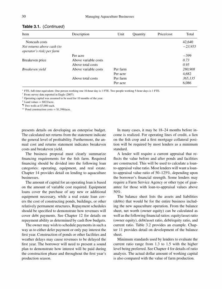
P1: SFK/UKS P2: SFK



Table 3.1. (Continued)


Noncash costs 42,640Net returns above cash (tooperator’s risk) per farm

−23,955

Per acre −399Breakeven price Above variable costs 0.73

Above total costs 0.95Breakeven yield Above variable costs Per farm 280,908

Per acre 4,682Above total costs Per farm 365,135

Per acre 6,086

∗ FTE, full-time equivalent. One person working one 10-hour day is 1 FTE. Two people working 5-hour days is 1 FTE.† From survey data reported in Engle (2007).‡ Operating capital was assumed to be used for 10 months of the year.§ Land values = $822/acre.¶ Two wells at $7,000 each.∗∗ Pond construction costs = $1,398/acre.

presents details on developing an enterprise budget.The calculated net returns from the statement indicatethe general level of profitability. Furthermore, the an-nual cost and returns statement indicates breakevencosts and breakeven yield.

The business proposal must clearly summarizefinancing requirements for the fish farm. Requiredfinancing should be divided into the following loancategories: operating, equipment, and real estate.Chapter 14 provides detail on lending to aquaculturebusinesses.

The amount of capital for an operating loan is basedon the amount of variable cost required. Equipmentloans cover the purchase of any new or additionalequipment necessary, while a real estate loan cov-ers the cost of constructing ponds, buildings, or otherrelatively permanent structures. Repayment schedulesshould be specified to demonstrate how revenues willcover debt payments. See Chapter 12 for details onrepayment ability as determined by cash flow budgets.

The owner may wish to schedule payments in such away as to either defer payment or only pay interest thefirst year. Construction of ponds or other facilities andweather delays may cause revenues to be delayed thefirst year. The borrower will need to present a soundplan to demonstrate how interest will be paid duringthe construction phase and throughout the first year’sproduction season.

In many cases, it may be 18–24 months before in-come is realized. For operating lines of credit, a lienon the fish crop and a first mortgage collateral posi-tion will be required by most lenders as a minimumstandard.

A lender will require a current appraisal that re-flects the value before and after ponds and facilitiesare constructed. This will be used to calculate a loan-to-appraisal value ratio. Most lenders will want a loan-to-appraisal value ratio of 50–125%, depending uponthe borrower’s financial strength. Some lenders mayrequire a Farm Service Agency or other type of guar-antee for those with loan-to-appraisal values above50%.

The balance sheet lists the assets and liabilities(debts) that would be for the entire business includ-ing the new aquaculture operation. From the balancesheet, net worth (owner equity) can be calculated aswell as the following financial ratios: equity/asset ratio(owner equity), debt/asset ratio, debt/equity ratio, andcurrent ratio. Table 3.2 provides an example. Chap-ter 11 provides detail on development of the balancesheet.

Minimum standards used by lenders to evaluate thecurrent ratio range from 1.3 to 1.5 with the higherlevel being preferred. See Chapter 4 for details of ratioanalysis. The actual dollar amount of working capitalis also compared with the value of farm production.

P1: SFK/UKS P2: SFK



Table 3.2. Balance Sheet for a 60-acreCatfish Farm, December 31.

Item Total value

Assets1. Current assets

Cash on deposit $3,715Fish inventory∗ $62,370

Total current assets $66,085

2. Noncurrent assetsEquipment $138,100Ponds $83,880Wells $14,000Land $49,320

Total noncurrent assets $285,300

3. Total assets $351,385Liabilities

4. Current liabilitiesPayments on debt due and payable

over next yearOperating loan interest $768Operating loan principal $41,046

Total current liabilities $41,814

5. Noncurrent liabilitiesEquipment loan $0Real estate loan $0

Total noncurrent liabilities $0

6. Total liabilities $41,8147. Net worth (3–6) $309,571

∗ 4,500 submarketable fish/acre at 0.33 lb each @ 0.70/lb.

The income statement itemizes anticipated farm in-come and expenses after the second full year of op-eration. The income statement is also called the profitand loss statement. Net farm income, return to capital,return to labor and management, and return to equityare calculated from the income statement. Table 3.3provides an example. See Chapter 11 for details ofdeveloping income statements.

A cash flow budget shows cash receipts and cash ex-penses by month, quarter, or year. It includes only cashexpenses and provides an indication of when cash willbe available for loan repayment. Table 3.4 provides anexample. See Chapter 12 for details on developmentof cash flow budgets.

The cash borrowing requirements projected by thecash flow budget must be examined carefully. Giventhe borrowing capacity of the farmer, can these bor-rowing requirements be met feasibly? Are there ways

Table 3.3. Income Statement for a 60-acreCatfish Farm, December 31.

Item Total value

Catfish farm revenueCash catfish sales $189,000

Total catfish farm revenue $189,000Catfish farm expenses

Cash operating expensesFeed $110,418Fingerlings $17,070Labor $6,643Plankton control $864Gas, fuel, and oil $7,800Electricity $17,340Repairs and maintenance $5,820Bird depredation supplies $375Seining and hauling $13,500Telephone $1,020Office supplies $660Legal/accounting $1,128Insurance $2,616

Total cash farm expenses $185,254Depreciation $14,110

Total operating expenses $199,364Cash interest paid

Interest on operating line of credit $10,744Interest paid on long-term loans

Land $4,932Wells $1,400Pond construction $8,388Equipment $13,810Total interest paid $39,274

Total expenses $238,638Net farm income from operations −$49,638Family labor $12,575Net returns to operator’s risk −$62,213

to restructure purchases or production to alleviate cashflow problems? An applicant needs to provide 3 yearsof tax records as well as 3 years (including a currentstatement) of financial statements.

Operating capacity and management skills will becritical to the success of a fish farming business. Ifthe owner does not have these skills, the business pro-posal must include funds to hire a manager or demon-strate that the owner has either taken or will be takingcourses in fish production. The resume should notethese courses along with experience raising fish thatincludes acreage managed, yields, stocking, and feed-ing rates, and hatchery experience.

P1: SFK/UKS P2: SFK


Tab

le3.

4.M

onth

lyC

ash

Flo

wB

udge

tfor

a60

-acr

eC

atfis

hFa

rmw

ithou

tFin

anci

ng.

Item

Janu

ary

Febr

uary

Mar

chA

pril

May

June

July

Aug

ust

Sept

embe

rO

ctob

erN

ovem

ber

Dec

embe

rTo

tal

Beg

inni

ngca

sh0

3,88

9−9

76−6

,136

16,1

1024

,826

19,5

885,

727

−5,6

03−1

6,45

31,

824

8,61

2Po

unds

ofca

tfish

sold

,lb

10,8

0010

,800

10,8

0048

,600

27,0

0027

,000

16,2

0027

,000

27,0

0045

,900

18,9

000

270,

000

Rec

eipt

sfr

omca

tfish

sold

,$7,

560

7,56

07,

560

34,0

2018

,900

18,9

0011

,340

18,9

0018

,900

32,1

3013

,230

018

9,00

0

Tota

lcas

hin

flow

7,56

011

,449

6,58

427

,884

35,0

1043

,726

30,9

2824

,627

13,2

9715

,677

15,0

548,

612

459,

000

Ope

rati

ngca

shex

pens

esFe

ed1,

105

2,20

92,

209

7,73

15,

522

17,6

6917

,669

22,0

8622

,086

6,62

63,

297

2,20

911

,041

8Fi

nger

lings

08,

535

8,53

50

00

00

00

00

17,0

70L

abor

,sea

sona

l,pa

rt-t

ime

00

00

996

1,66

11,

661

1,66

166

40

00

6,64

3

Plan

kton

cont

rol

00

00

216

021

60

432

00

086

4

Gas

,die

self

uel,

and

oil

468

234

234

234

390

624

1,01

41,

014

1,24

81,

248

546

546

7,80

0

Ele

ctri

city

347

347

520

694

867

1,73

42,

601

2,94

82,

948

2,94

886

752

017

,341

Rep

airs

and

mai

nten

ance

698

116

233

233

291

587

757

757

582

291

291

989

5,82

0

Bir

dde

pred

atio

n56

5656

3819

00

00

3856

5637

5Se

inin

gan

dha

ulin

g54

054

054

02,

430

1,35

01,

350

810

1,35

01,

350

2,29

594

50

13,5

00

Tele

phon

e82

8261

102

102

8282

8282

8282

102

1,02

0O

ffice

supp

lies

537

3313

132

132

6633

3326

3399

660

Farm

insu

ranc

e20

920

920

920

920

920

923

520

923

520

923

523

52,

616

Leg

al/

acco

untin

g11

390

9090

9090

9090

9090

9011

31,

128

Tota

lope

ratin

gex

pens

es3,

671

12,4

2512

,720

11,7

7410

,184

24,1

3825

,201

30,2

3029

,750

13,8

536,

442

4,86

918

5,25

5

P1: SFK/UKS P2: SFK


Deb

tser

vici

ngR

eale

stat

eIn

tere

st0

00

00

00

00

00

00

Prin

cipa

l0

00

00

00

00

00

00

Subt

otal

00

00

00

00

00

00

0E

quip

men

tIn

tere

st0

00

00

00

00

00

00

Prin

cipa

l0

00

00

00

00

00

00

Subt

otal

00

00

00

00

00

00

0O

pera

ting

Inte

rest

00

00

00

00

00

00

0Pr

inci

pal

00

00

00

00

00

00

0Su

btot

al0

00

00

00

00

00

00

Tota

ldeb

tse

rvic

ing

00

00

00

00

00

00

0

Tota

lcas

hou

tflow

3,67

112

,425

12,7

2011

,774

1,01

8424

,138

25,2

0130

,230

29,7

5013

,853

6,44

24,

869

18,5

255

Cas

h avai

labl

e3,

889

−976

−6,1

3616

,110

24,8

2619

,588

5,72

7−5

,603

−16,

453

1,82

48,

612

3,74

327

3,74

5

New bo

rrow

ing

00

00

00

00

00

00

0

End

ing

cash

bala

nce

3,88

9−9

76−6

,136

16,1

1024

,826

19,5

885,

727

−5,6

03−1

6,45

31,

824

8,61

23,

743

273,

745

Sum

mar

yof

debt

outs

tand

ing

Rea

lest

ate

Equ

ipm

ent

Ope

ratin

g

P1: SFK/UKS P2: SFK



REVISIONS TO THE BUSINESS PLAN

The plan must also include a detailed methodologyfor monitoring and evaluating the company’s perfor-mance once the plan is put into place. The business plantypically will need to be revised following the evalua-tion of the marketing and production plans developed.Problems detected in cash flow, in financial strength,borrowing capacity, or overall feasibility require thatthe proposed business be modified to overcome theseproblems. Once modifications are proposed, then themarketing and production plans and financial state-ments must also be revised and reanalyzed to see if themodifications made have resolved the problems.

Ideally, the best would be to analyze all alterna-tive strategies with potential to achieve the goals andobjectives of the business. In reality, few aquaculturebusinesses have the capability to do this. Thus, the it-erative process suggested above may be more practicalfor many farmers.

EVALUATION OF A LOAN PROPOSAL

In evaluating a business proposal and loan application,lenders will take into consideration several factors.The overall character and honesty of the individual isconsidered on the basis of his or her history of pay-ing other bills and character references. Owner equity,the current ratio (from the balance sheet), the loan-to-appraisal value, and the value of farm production arekey indicators for many lenders. Earnings will be ex-amined in great detail along with repayment capacity.These will be viewed in terms of sustaining produc-tion over a 3-year price cycle. Collateral and capital ofthe individual operator will also affect the level of thelender’s decision. The lender will look at the financialcondition of the processor to make certain that the pro-ducer will receive payment within 2–3 weeks of fishdelivery. A comprehensive and thorough proposal willgreatly facilitate the loan application process.

RECORD-KEEPING

A business plan requires detailed records on everyphase of the business, from production and marketingdata to complete financial information. The most use-ful data are longer-term series of price and cost data.These provide for trend analyses and indicate whereprices and costs are headed for better planning.

Detailed market information is also valuable. Main-taining files of market reports and changing conditions

is a good basis for developing the marketing plan por-tion of the business plan.


Tables 3.1–3.4 present the financial analyses for a60-acre catfish farm in the United States. This farmplans to sell food-sized fish to a processing plant. Thefarm’s production technology is the same as that of the256-acre farm for which financial statements are pre-sented in Chapters 10–12. For comparison betweenthe two farm sizes, Table 3.5 summarizes key finan-cial indicators for a 256-acre farm, demonstrating itsfinancial feasibility.

The 60-acre farm is facing a different set of cir-cumstances from those of the 256-acre farm. Feed andenergy prices have escalated rapidly but fish priceshave not. Thus, Tables 3.1 and 3.3 shows that this farmis not profitable. Its balance sheet (Table 3.2) showsa high net worth. This is primarily because the farmused its own capital, borrowing the operating capitalnecessary for cash flow. However, the cash flow budget(Table 3.4) shows that there are cash shortfalls in themonths of February, March, August, and September.Thus, new borrowing will be needed in these months.The new borrowing results in adequate cash flow (Ta-ble 3.6), but incurs an operating loan of $48,068 andan outstanding operating loan of $7,022 at the end ofthe year. Thus, with the operating loan, this farm canmake its payments in the short term.

However, few farms can provide all the investmentcapital needed. If the farm has to borrow just 30%of the capital needed to purchase the equipment, buythe land, and build the ponds, the cash flow changessubstantially. Table 3.7 shows that less of the operat-ing loan was paid off throughout the year, leaving anoperating loan balance of $22,030 that will need tobe carried over until the next year. Thus, this farm hasproblems of profitability as well as cash flow problemsif even just 30% of the long-term capital is borrowed.

This farm will need to make some adjustments.Breakeven price of catfish sold above total costs fromthe enterprise budget is $0.95. The farm will need toexplore some alternative markets to see if developinga live market can result in achieving a higher price.Careful analysis will be needed to determine the vol-ume of fish likely to be sold as a live product. In someareas, live catfish are sold for as much as $1.00/lb,but volumes tend to be only a few thousand poundsa week. Alternatively, the farm may need to look atthe feasibility of either expanding its size to capture

P1: SFK/UKS P2: SFK



Table 3.5. Summary of Results of Financial Analyses of 256-acre Catfish Farm Example.

Analysis Unit Farm value Per-acre valueSource (table inthis volume)

Enterprise budgetNet returns to operator’s risk $ −$18,502 −$72 Table 10.2Net returns to operator’s labor, management,and risk

$ $2,792 $11 Table 10.2

Breakeven price above variable costs $/lb $0.57 $0.57 Table 10.2Breakeven price above total costs $/lb $0.72 $0.72 Table 10.2Breakeven yield above variable costs lb/acre 932,104 3,641 Table 10.2Breakeven yield above total costs lb/acre 1,178,431 4,603 Table 10.2

Balance sheetTotal current assets $ $281,961 1,101 Table 11.1Total noncurrent assets $ $1,003,890 3,921 Table 11.1Total assets $ $1,285,851 5,023 Table 11.1Total current liabilities $ $110,584 432 Table 11.1Total noncurrent liabilities $ $423,630 1,655 Table 11.1Total liabilities $ $534,214 2,087 Table 11.1Net worth $ $751,637 2,936 Table 11.1

Income statementNet farm income from operations $ $2,792 10.91 Table 11.2

Cash flow budgetCash available $ Increasing

acrossmonths

n.a.∗ Table 12.1

New borrowing $ 0 n.a.∗ Table 12.1Debt outstanding $ 0 n.a.∗ Table 12.1

∗ Not applicable to a cash flow budget.

economies of scale or to decrease its size to focus onproducing the volumes that local live markets can bear.Complete financial analyses are needed for each newscenario to judge its feasibility.


Engle and Neira (2005) developed a series of pro formafinancial statements for tilapia businesses in Kenya.Data were collected from tilapia farms in Kenya fromwhich sample enterprise budgets were developed. Thebase enterprise budget for a 1-ha tilapia farm in Kenyawas based on a stocking rate of 3.0 tilapia/m2. Fishwere assumed to be fed a pelleted diet. The enter-prise was profitable, with positive net returns. The in-come statement also demonstrated profitability withpositive net farm income. The balance sheet showedpositive owner equity, indicating a strong financial po-sition. The cash flow budget showed a positive cashflow balance, with an ending cash balance greater than

the beginning cash balance. Overall, the business planshowed that the overall plan is feasible.

SUMMARY

This chapter presents an outline of the content of athorough business plan. Aquaculture businesses aresophisticated and capital-intensive businesses. Prepa-ration of a comprehensive plan can help the ownerto avoid major problems or redirect the business in amanner that is likelier to succeed.

REVIEW QUESTIONS

1. Why is a business plan important?

2. What is the difference between a business planand a business loan proposal?

3. What are the major components of a businessplan?

P1: SFK/UKS P2: SFK


Tab

le3.

6.M

onth

lyC

ash

Flo

wB

udge

tfor

a60

-acr

eC

atfis

hFa

rmw

ithN

ewB

orro

win

gfr

oman

Ope

ratin

gLo

an.

Item

Janu

ary

Febr

uary

Mar

chA

pril

May

June

July

Aug

ust

Sept

embe

rO

ctob

erN

ovem

ber

Dec

embe

rTo

tal

Beg

inni

ngca

sh0

10,0

0010

,000

10,0

0015

,832

24,5

4819

,310

10,0

0010

,000

10,0

0010

,000

10,0

00Po

unds

ofca

tfish

sold

,lb

10,8

0010

,800

10,8

0048

,600

27,0

0027

,000

16,2

0027

,000

27,0

0045

,900

18,9

000

270,

000

Rec

eipt

sfr

omca

tfish

sold

,$7,

560

7,56

07,

560

34,0

2018

,900

18,9

0011

,340

18,9

0018

,900

32,1

3013

,230

018

9,00

0

Tota

lcas

hin

flow

7,56

017

,560

17,5

6044

,020

34,7

3243

,448

30,6

5028

,900

28,9

0042

,130

23,2

3010

,000

459,

000

Ope

rati

ngca

shex

pens

esFe

ed1,

105

2,20

92,

209

7,73

15,

522

17,6

6917

,669

22,0

8622

,086

6,62

63,

297

2,20

911

0,41

8Fi

nger

lings

08,

535

8,53

50

00

00

00

00

17,0

70L

abor

,sea

sona

l,pa

rt-t

ime

00

00

996

1,66

11,

661

1,66

166

40

00

6,64

3

Plan

kton

cont

rol

00

00

216

021

60

432

00

086

4G

as,d

iese

lfue

l,an

doi

l46

823

423

423

439

062

41,

014

1,01

41,

248

1,24

854

654

67,

800

Ele

ctri

city

347

347

520

694

867

1734

2,60

12,

948

2,94

82,

948

867

520

17,3

41R

epai

rsan

dm

aint

enan

ce69

811

623

323

329

158

775

775

758

229

129

198

95,

820

Bir

dde

pred

atio

n56

5656

3819

00

00

3856

5637

5Se

inin

gan

dha

ulin

g54

054

054

02,

430

1,35

01,

350

810

1,35

01,

350

2,29

594

50

13,5

00

Tele

phon

e82

8261

102

102

8282

8282

8282

102

1,02

0O

ffice

supp

lies

537

3313

132

132

6633

3326

3399

660

Farm

insu

ranc

e20

920

920

920

920

920

923

520

923

520

923

523

52,

616

Leg

al/

acco

untin

g11

390

9090

9090

9090

9090

9011

31,

128

Tota

lope

ratin

gex

pens

es3,

671

12,4

2512

,720

11,7

7410

,184

24,1

3825

,201

30,2

3029

,750

13,8

536,

442

4,86

918

5,25

5

P1: SFK/UKS P2: SFK


Deb

tser

vici

ngR

eale

stat

eIn

tere

st0

00

00

00

00

00

00

Prin

cipa

l0

00

00

00

00

00

00

Subt

otal

00

00

00

00

00

00

0E

quip

men

tIn

tere

st0

00

00

00

00

00

00

Prin

cipa

l0

00

00

00

00

00

00

Subt

otal

00

00

00

00

00

00

0O

pera

ting Inte

rest

051

9213

60

00

3813

322

474

1876

5Pr

inci

pal

00

016

,279

00

00

018

,053

6,71

40

41,0

46Su

btot

al0

5192

16,4

150

00

3813

318

,277

6,78

818

41,8

11To

tald

ebt

serv

icin

g0

5192

16,4

150

00

3813

318

,277

6,78

818

41,8

11

Tota

lcas

hou

tflow

3,67

112

,476

12,8

1228

,189

10,1

8424

,138

25,2

0130

,268

29,8

8332

,130

13,2

304,

887

227,

065.

8C

ash

avai

labl

e3,

889

5,08

44,

748

15,8

3224

,548

19,3

105,

449

−1,3

68−9

8310

,000

10,0

005,

113

231,

934

New

borr

owin

g6,

111

4,91

65,

252

00

04,

551

11,3

6810

,983

00

4,88

748

,068

End

ing

cash

bala

nce

10,0

0010

,000

10,0

0015

,832

24,5

4819

,310

10,0

0010

,000

10,0

0010

,000

10,0

0010

,000

280,

002

Sum

mar

yof

debt

outs

tand

ing

Rea

lest

ate

Equ

ipm

ent

Ope

ratin

g6,

111

11,0

2716

,279

00

04,

551

15,9

1926

,902

8,84

92,

135

7,02

2

P1: SFK/UKS P2: SFK


Tab

le3.

7.M

onth

lyC

ash

Flo

wB

udge

tfor

a60

-acr

eC

atfis

hFa

rmw

ithN

ewB

orro

win

gfr

oman

Ope

ratin

gLo

anan

d30

%B

orro

win

gfo

rE

quip

men

tand

Rea

lEst

ate

Cap

ital.

Item

Janu

ary

Febr

uary

Mar

chA

pril

May

June

July

Aug

ust

Sept

embe

rO

ctob

erN

ovem

ber

Dec

embe

rTo

tal

Beg

inni

ngca

sh0

10,0

0010

,000

10,0

0015

,832

24,5

4819

,310

10,0

0010

,000

10,0

0010

,000

10,0

00Po

unds

ofca

tfish

sold

,lb

10,8

0010

,800

10,8

0048

,600

27,0

0027

,000

16,2

0027

,000

27,0

0045

,900

18,9

000

270,

000

Rec

eipt

sfr

omca

tfish

sold

,$7,

560

7,56

07,

560

34,0

2018

,900

18,9

0011

,340

18,9

0018

,900

32,1

3013

,230

018

9,00

0

Tota

lcas

hin

flow

7,56

017

,560

17,5

6044

,020

34,7

3243

,448

30,6

5028

,900

28,9

0042

,130

23,2

3010

,000

459,

000

Ope

rati

ngca

shex

pens

esFe

ed1,

105

2,20

92,

209

7,73

15,

522

17,6

6917

,669

22,0

8622

,086

6,62

63,

297

2,20

911

0,41

8Fi

nger

lings

08,

535

8,53

50

00

00

00

00

17,0

70L

abor

,sea

sona

l,pa

rt-t

ime

00

00

996

1,66

11,

661

1,66

166

40

00

6,64

3

Plan

kton

cont

rol

00

00

216

021

60

432

00

086

4G

as,d

iese

lfue

l,an

doi

l46

823

423

423

439

062

41,

014

1,01

41,

248

1,24

854

654

67,

800

Ele

ctri

city

347

347

520

694

867

1,73

42,

601

2,94

82,

948

2,94

886

752

017

,340

Rep

airs

and

mai

nten

ance

698

116

233

233

291

587

757

757

582

291

291

989

5,82

0

Bir

dde

pred

atio

n56

5656

3819

00

00

3856

5637

5Se

inin

gan

dha

ulin

g54

054

054

02,

430

1,35

01,

350

810

1,35

01,

350

2,29

594

50

13,5

00

Tele

phon

e82

8261

102

102

8282

8282

8282

102

1,02

0O

ffice

supp

lies

537

3313

132

132

6633

3326

3399

660

Farm

insu

ranc

e20

920

920

920

920

920

923

520

923

520

923

523

52,

616

Leg

al/

acco

untin

g11

390

9090

9090

9090

9090

9011

31,

128

Tota

lope

ratin

gex

pens

es3,

671

12,4

2512

,720

11,7

7410

,184

24,1

3825

,201

30,2

3029

,750

13,8

536,

442

4,86

918

5,25

4

P1: SFK/UKS P2: SFK


Deb

tser

vici

ngR

eale

stat

eIn

tere

st0

00

00

00

00

092

20

0Pr

inci

pal

00

00

00

00

00

3,94

30

0Su

btot

al0

00

00

00

00

04,

865

00

Equ

ipm

ent

Inte

rest

00

00

00

00

01,

650

00

0Pr

inci

pal

00

00

00

00

08,

286

00

0Su

btot

al0

00

00

00

00

9,93

60

00

Ope

ratin

gIn

tere

st0

5192

136

00

038

133

224

157

142

972

Prin

cipa

l0

00

16,2

790

00

00

8,11

71,

766

3526

,197

Subt

otal

051

9216

,415

00

038

133

8,34

11,

923

177

27,1

69To

tald

ebt

serv

icin

g0

5192

16,4

150

00

3813

318

,277

6,78

817

741

,970

Tota

lcas

hou

tflow

3,67

112

,476

12,8

1228

,189

10,1

8424

,138

25,2

0130

,268

29,8

8332

,130

13,2

305,

046

227,

223.

6C

ash

avai

labl

e3,

889

5,08

44,

748

15,8

3224

,548

19,3

105,

449

−1,3

68−9

8310

,000

10,0

004,

954

231,

776

New

borr

owin

g6,

111

4,91

65,

252

00

04,

551

11,3

6810

,983

00

5,04

648

,227

End

ing

cash

bala

nce

10,0

0010

,000

10,0

0015

,832

24,5

4819

,310

10,0

0010

,000

10,0

0010

,000

10,0

0010

,000

280,

003

Sum

mar

yof

debt

outs

tand

ing

Rea

lest

ate

48,5

7648

,576

48,5

7648

,576

48,5

7648

,576

48,5

7648

,576

48,5

7648

,576

44,6

3344

,633

Equ

ipm

ent

41,4

3041

,430

41,4

3041

,430

41,4

3041

,430

41,4

3041

,430

41,4

3033

,144

33,1

4433

,144

Ope

ratin

g6,

111

11,0

2716

,279

00

04,

551

15,9

1926

,902

18,7

8517

,019

22,0

30

P1: SFK/UKS P2: SFK



4. What is the difference between a commodity anda niche market?

5. Why does business planning take so much time?

6. Describe several examples of the types of exter-nal and internal opportunities that can affect anaquaculture business.

7. Describe several examples of the types of externaland internal threats that can affect an aquaculturebusiness.

8. What are the major components of the marketingplan for the business?

9. Outline the content of the production plan thatmust be included in a complete business plan.

10. What types of resources are available for devel-oping aquaculture business plans?

REFERENCES

Engle, Carole R. 2007. Arkansas Catfish Produc-tion Budgets. Arkansas Cooperative ExtensionProgram MP466. Pine Bluff, AR: University ofArkansas.

Engle, Carole R. and Ivano Neira. 2005. Tilapia FarmBusiness Management and Economics. Corvallis,OR: Oregon State University.

Engle, Carole R. and Kwamena Quagrainie. 2006.The Aquaculture Marketing Handbook. Ames, IA:Blackwell Publishing.

Morris, J.E. 1994. Niche Marketing Your AquacultureProducts. Publication #TB-107. Ames, IA: IowaState University Press.

Palfreman, Andrew. 1999. Fish Business Management.Oxford: Blackwell Science.

SUGGESTED REFERENCES

Barry, Peter J., John A. Hopkin, and C.B. Baker. Fi-nancial Management in Agriculture. Danville, IL:The Interstate Printers & Publishers.

Furlong, Carla B. 1993. Marketing for Keeps: BuildingYour Business by Retaining Your Customers. NewYork: John Wiley & Sons.

Kay, Ronald D., William M. Edwards, and Patricia A.Duffy. 2008. Farm Management, 6th ed. New York:McGraw-Hill.

Lee, Warren F., Michael D. Boehlje, Aaron G. Nelson,William G. Murray. 1988. Agricultural Finance, 8thed. Ames, IA: Iowa State University Press.

Libbin, James D., Lowell B. Catlett, and Michael L.Jones. 1994. Cash Flow Planning in Agriculture.Ames, IA: Iowa State University Press.

O’Hara, Patrick D. 1989. SBA Loans. New York: JohnWiley & Sons.

Olson, Kent D. 2004. Farm Management Principlesand Strategies. Ames, IA: Iowa State UniversityPress.

Rachlin, Robert and Allen H.W. Sweeny. 1993. Hand-book of Budgeting, 3rd ed. New York: John Wiley& Sons.

Warren, Martyn. 1998. Financial Management forFarmers and Rural Managers, 4th ed. Ames, IA:Blackwell Science.

P1: SFK/UKS P2: SFK


4Monitoring Economic andFinancial Performance ofAquaculture Businesses

Efficient management of a farm can make the differ-ence between profits and losses especially in years withunfavorable prices and costs. However, farm manage-ment involves more than just taking care of the bi-ological processes involved; it includes paying closeattention to economic and financial measures of thefarm business. Few farmers enjoy spending time onfinancial analysis, but doing so is essential to the suc-cess of the business. Even if the business retains an ac-counting firm to generate the analyses, spending timeto use the results to plan to make improvements isnecessary.

Chapter 3 described the process of developinga comprehensive plan for the aquaculture business.Having the plan developed is a first step, but theowner/manager must follow up on the plan each yearwith equally careful analysis and assessment of theperformance of the business over the past year. Thisanalysis should go through the entire plan to assesswhether the short-term goals for that year were metor not. There are a series of biological, economic, andfinancial ratios and indicators that can be used to iden-tify why goals were not met and (or if they were)to further evaluate the business’s performance over theyear. From this evaluation, new goals for the upcomingyear must be developed and the overall plan modifiedas appropriate, to keep the business on track to meetits longer-term goals.

Solvency and liquidity are important financial mea-sures of the overall well being of a business. Solvencyrefers to the value of the assets owned by the business

as compared to the amount of liabilities. Assets refer tothe value of anything owned by the business whereasliabilities refer to any debt obligations that the businesshas outstanding. Liquidity refers to the ability of a busi-ness to meet cash flow obligations. Liquidity is criticalfor the financial transactions of the business to runsmoothly. The balance sheet and income statementsare used as the bases for measuring and monitoringsolvency and liquidity in the farm business. For detailson developing balance sheets and income statements,see Chapter 11 of this book. This chapter reviews anddiscusses various types of economic and financial in-dicators that can be used to measure performance ofthe aquaculture business.

PRODUCTION AND INPUT USEEFFICIENCY

Production Efficiency

Production efficiency refers to the biological perfor-mance of the farm. Monitoring the efficiency of theaquaculture business begins with evaluating these bio-logical factors. The first such measure to monitor is thetotal production from the farm, or gross yield. Grossyield is measured in weight of the production per unitarea (lb/acre or kg/ha for pond production and lb/cubicfoot or kg/cubic meters for cages). Net yield is the grossyield minus the weight of the fingerlings or postlarvaestocked. In Table 4.1, the gross yield of catfish was4,500 lb/acre while net yield, after subtracting out theweight of fingerlings stocked was 4,318 lb/acre. Overtime, increases in gross and net yield will result inreduced production costs and greater productivity.


41

P1: SFK/UKS P2: SFK



Table 4.1. Production Efficiency Measures, 256-acre Catfish Farm.

Measure Calculation Unit Farm value

Gross yield Weight of fish sold ÷ number of acres lb/acre 4,500Net yield (Weight of fish sold − weight (lb) of fish stocked) ÷

number of acreslb/acre 4,318

Survival (Number of fish sold ÷ number of fish stocked) × 100 % 79%Average size of fish harvested Weight of fish harvested ÷ number of fish harvested lb 1.5Growth rate (Average size of fish harvested − average size of fish

stocked) ÷ number of days of productiong/day 2.2

Net yield measures the gain in production over timeand is the more accurate measure of biological effi-ciency. Gross yield is the weight sold and is used tocalculate the total revenue for the business. Monitor-ing yields following management changes on the farmwill provide a basis for understanding the effects ofthe change.

Measuring and monitoring survival from year toyear provides an indication of the effectiveness of themeasures undertaken to control and minimize mortal-ities. These may include disease control and predatorcontrol measures. Table 4.1 shows a survival of 74%for the 256-acre catfish farm. Improving survival willincrease profits and will improve other financial indi-cators as discussed below.

Records maintained on the farm must also look atthe average size of fish harvested. Changes in the av-erage size of fish harvested each year can provide anindication of effects of other management changes onthe farm, such as changes in the stocking density. Sizethresholds may have implications for prices paid forvarious size groups of fish. Table 4.1 shows an averagesize of fish harvested of 1.5 lb. Decreases in the averageweight of fish sold might indicate inefficient gradingand sales of larger numbers of submarket sized fishwhile increases in the average weight might indicateinefficient harvesting (growing numbers of larger fishthat had previously escaped the seine).

Growth rates are an important indicator also, but canbe difficult or impossible to calculate for farms that arein continuous production. Increasing growth rates willincrease turnover rates, can improve cash flow, and arelikely to increase profitability.

Input Use Efficiency

Measures of the efficiency of input use should also beused to evaluate and monitor farm efficiency. The feed

conversion ratio (FCR) is the most important measureof input use efficiency, but similar measures can becalculated for labor, utility use, and other inputs. FCRis the most important for many aquaculture businessesbecause feed is the largest single cost on many aqua-culture farms. Efficient use of feed inputs will assistthe farmer to keep costs per unit of fish produced aslow as possible. Table 4.2 shows a FCR of 2.12 forthe 256-acre catfish farm. If this farm could reduce itsFCR across the farm to 2.0, its total costs would bereduced by 2.2%, but net farm income would increasesevenfold, to $20,450 from $2,792.

It can be instructive to also calculate similar mea-sures for other inputs, particularly for businesses inwhich an input other than feed is the most important.These can include fish production per worker (effi-ciency of labor), fish production per dollar of work-ing capital (efficiency of operating capital), and fishproduction per 1,000 fingerlings stocked (efficiencyof fingerlings stocked). For the example farm, the in-put use efficiency measures were: 791 (fingerling effi-ciency), 6.72 (operating capital efficiency), and 1,800(labor efficiency) (Table 4.2). Year-to-year monitoringof these efficiency measures will demonstrate whetherthese measures show improvement or decline. For ex-ample, purchasing an improved strain of fish wouldbe expected to result in improved fingerling efficiency,while hiring new workers may result in improved laborefficiency. Conversely, if fingerling efficiency declinesafter purchase of a more expensive, improved strain,it would be advantageous to discontinue expenditureson it.

The farm manager should review the measures ofinput use efficiency at least once a year and comparethem with previous years. The remainder of this chap-ter concentrates on economic and financial measuresthat are less commonly used by aquaculture farm man-agers.

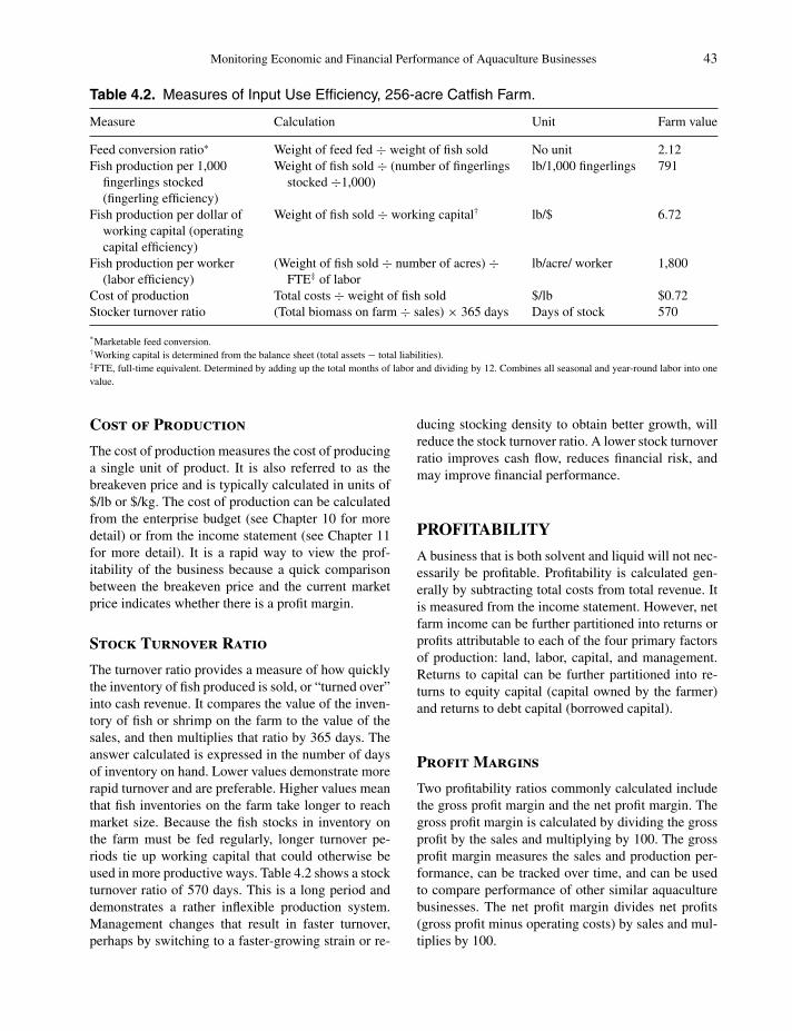
P1: SFK/UKS P2: SFK


Monitoring Economic and Financial Performance of Aquaculture Businesses 43

Table 4.2. Measures of Input Use Efficiency, 256-acre Catfish Farm.


Feed conversion ratio∗ Weight of feed fed ÷ weight of fish sold No unit 2.12Fish production per 1,000

fingerlings stocked(fingerling efficiency)

Weight of fish sold ÷ (number of fingerlingsstocked ÷1,000)

lb/1,000 fingerlings 791

Fish production per dollar ofworking capital (operatingcapital efficiency)

Weight of fish sold ÷ working capital† lb/$ 6.72

Fish production per worker(labor efficiency)

(Weight of fish sold ÷ number of acres) ÷FTE‡ of labor

lb/acre/ worker 1,800

Cost of production Total costs ÷ weight of fish sold $/lb $0.72Stocker turnover ratio (Total biomass on farm ÷ sales) × 365 days Days of stock 570

*Marketable feed conversion.†Working capital is determined from the balance sheet (total assets − total liabilities).‡FTE, full-time equivalent. Determined by adding up the total months of labor and dividing by 12. Combines all seasonal and year-round labor into onevalue.

Cost of Production

The cost of production measures the cost of producinga single unit of product. It is also referred to as thebreakeven price and is typically calculated in units of$/lb or $/kg. The cost of production can be calculatedfrom the enterprise budget (see Chapter 10 for moredetail) or from the income statement (see Chapter 11for more detail). It is a rapid way to view the prof-itability of the business because a quick comparisonbetween the breakeven price and the current marketprice indicates whether there is a profit margin.

Stock Turnover Ratio

The turnover ratio provides a measure of how quicklythe inventory of fish produced is sold, or “turned over”into cash revenue. It compares the value of the inven-tory of fish or shrimp on the farm to the value of thesales, and then multiplies that ratio by 365 days. Theanswer calculated is expressed in the number of daysof inventory on hand. Lower values demonstrate morerapid turnover and are preferable. Higher values meanthat fish inventories on the farm take longer to reachmarket size. Because the fish stocks in inventory onthe farm must be fed regularly, longer turnover pe-riods tie up working capital that could otherwise beused in more productive ways. Table 4.2 shows a stockturnover ratio of 570 days. This is a long period anddemonstrates a rather inflexible production system.Management changes that result in faster turnover,perhaps by switching to a faster-growing strain or re-

ducing stocking density to obtain better growth, willreduce the stock turnover ratio. A lower stock turnoverratio improves cash flow, reduces financial risk, andmay improve financial performance.

PROFITABILITY

A business that is both solvent and liquid will not nec-essarily be profitable. Profitability is calculated gen-erally by subtracting total costs from total revenue. Itis measured from the income statement. However, netfarm income can be further partitioned into returns orprofits attributable to each of the four primary factorsof production: land, labor, capital, and management.Returns to capital can be further partitioned into re-turns to equity capital (capital owned by the farmer)and returns to debt capital (borrowed capital).

Profit Margins

Two profitability ratios commonly calculated includethe gross profit margin and the net profit margin. Thegross profit margin is calculated by dividing the grossprofit by the sales and multiplying by 100. The grossprofit margin measures the sales and production per-formance, can be tracked over time, and can be usedto compare performance of other similar aquaculturebusinesses. The net profit margin divides net profits(gross profit minus operating costs) by sales and mul-tiplies by 100.

P1: SFK/UKS P2: SFK



Net Farm Income

The primary measure of farm profitability is net farmincome. Net farm income measures the return to oper-ator’s equity, capital, unpaid labor, and management.It is measured from the income statement. Net farmincome is measured as follows:

Total revenue − total expenses= net farm income from operations± the gain/loss on the sale of capital assets= net farm income

For the example farm, net farm income from the in-come statement for the 256-acre catfish farm is $2,792(Table 4.3; Chapter 11). This farm will need to improveits low net farm income over time to provide adequatecompensation for the owners.

Rate of Return on Farm Assets

The rate of return on farm assets (ROA) measures theprofits obtained from the use of all capital (debt andequity capital) invested in the business and can be com-pared to rates of return on other long-term investments.It has several names including rate of return on assets(ROA), return on assets (ROA), return to capital, andreturn on investment (ROI). It can be viewed as aninterest rate earned on the total investment of capitalin the farm. It is a measure of profitability because itcompares the profits (returns minus expenses) to thevalue of the assets of the business. If the farm main-tains a beginning and ending balance sheet for eachyear, the value of the total assets is averaged betweenthe beginning and end-of-year balance sheet. The ROAis not related to the way that assets are financed.

The ROA is independent of the type and amount offinancing. It can be compared to other similar farms,returns from other investments, opportunity costs ofthe farm’s capital, and past ROA values for the farm tomeasure profitability.

ROA is calculated as follows:

ROA = return to assets

average asset value× 100 (4.1)

Return to assets is calculated as follows:

Adjusted net farm income(= net farm income from operations plus interest

expenses)− opportunity cost of unpaid labor− opportunity cost of management= return to assets

Interest is added back to net farm income (in the cal-culation of adjusted net farm income) because interestexpenses were subtracted out in the income statement.This is because the ROA measures the return to allcapital used; if interest has been charged out for theuse of the capital, then the returns are to the equityalone, not the total amount of capital used. In otherwords, the use of the capital would have been chargedout twice and would give a false measure of the profitsgenerated by the capital used in the business.

In calculating the ROA, adjustments are also madefor unpaid labor and management that is provided bythe farm owner and family. If not subtracted out, thenthe calculation of net farm income would include theearnings produced by the farm labor and management.Because wages were not paid directly to the familylabor and management, opportunity costs are used toassign a value to these resources. The ROA is an aver-age return and should not be used to make investmentdecisions. Chapter 13 provides details on the appro-priate tools for assessing investment decisions.

In Table 4.3, the ROA for the example farm is 10%.Rates of return in agriculture are frequently lower thanfor other types of businesses. An ROA of 10% is com-petitive for many agriculture enterprises, particularlyduring times when interest rates are low.

Operating Profit Margin Ratio

The operating profit margin ratio (OPMR) measuresthe proportion of gross revenues left after paying ex-penses by calculating operating profit as a percent oftotal revenue. The indicator measures the operatingefficiency of the business. It is calculated as:

OPMR = return to farm assets

gross revenue of farm(4.2)

The higher the value, the more profit the businesshas generated per dollar of revenue. Farms with largeinvestments in fixed assets such as land and few operat-ing expenses will show a higher OPMR. A high OPMRresults from a business that maintains expenses in pro-portion to the value of the farm’s production. Farmswith more rented assets will have a higher ROA buta lower OPMR. Problems of profitability arise whenboth the ROA and OPMR are below average. A lowOPMR indicates that more attention must be paid toimproving this ratio before looking at expanding pro-duction levels. Low OPMRs can result from inefficientproduction, low prices, or high operating expenses.

P1: SFK/UKS P2: SFK



Table 4.3. Profitability Measures, 256-acre Catfish Farm.


Net farm income Total revenue − total expenses= net farm income from operations± gain or loss on sale of capital assets

$ 2,792

Rate of return on assets (%) Net farm income+ interest expense= adjusted net farm income− operating cost of unpaid labor− operating cost of management= return to assetsROA = return to assets ÷ average farm asset

value∗ × 100

$$$$$$%

2,792150,579153,37110,14011,154132,07710%

Rate of return on equity (%) Net farm income− operating cost of unpaid labor− operating cost of management= return on equityROE = return on equity ÷ average equity† ×

100%

$$$$

2,79210,14011,154−18,502−2%

Operating profit margin ratio Net farm income+ interest− operating cost of unpaid labor− operating cost of management= operating profitOperating profit margin ratio= operating profit ÷ total revenue × 100%

$$$$$$%

2,792150,57910,14011,154132,077132,07716%

Financial leverage ratio ROE ÷ ROA % −0.2%Return to labor and

managementNet farm income from operations+ interest expenses= adjusted net farm income− operating cost of all capital (10%)

$

$$$$

24,786 =

2,792150,579153,371128,585

Return to laborReturn to labor and management

− operating cost of management

$$

$13,632 =$24,786−$11,154

Return to managementReturn to labor and management

− operating cost of labor

$$

$14,646 =$24,786−$10,140

*Average farm asset value is the average of the beginning and ending value of total asset values from the farm’s balance sheet. In this exampleof the 256-acre catfish farm, the total asset value is $1,285,851 found on Table 11.1 on the balance sheet of the farm. For this example, in theabsence of beginning (January 1) and ending (December 31) balance sheets, the simplifying assumption is that this value did not change over theyear.†Average farm equity is the average of the beginning and ending value of net worth, from the farm’s balance sheet. In this example of the 256-acrecatfish farm, the net worth (owner’s equity) is $751,637 found on Table 11.1 on the balance sheet of the farm. For this example, in the absence ofseparate beginning (January 1) and ending (December 31) balance sheets, the simplifying assumption used is that this value did not change over theyear.

P1: SFK/UKS P2: SFK



The OPMR for the example 256-acre catfish farm is16%. This indicates that, for every dollar of revenue,$0.16 remains as profit after paying the operating ex-penses needed to generate that dollar.

Rate of Return on Farm Equity

The rate of return on farm equity (ROE) measures thereturns on the owner’s share of capital (equity) usedin the business. It can be viewed as an interest rateearned on the business’ average equity or net worth. Itis indicative of the farm’s financial progress because,if the business should fail, the equity capital will bewhat the farmer has left after paying off all liabilities.It measures the percent return to owner’s net worth orequity. If the farm has no debt, the ROE is equal to theROA. It is calculated as:

ROE = return on equity

average equity× 100 (4.3)

The ROE is calculated as follows:

Net farm income from operations− opportunity cost of unpaid labor− opportunity cost of management= return on equity

In contrast to the calculation of the ROA, interestcharges are not added back in to net farm income fromoperations to calculate the return on equity. This is be-cause interest is a charge on borrowed capital. BecauseROE measures only the return to equity capital, it iscorrect to have charged out the interest cost on bor-rowed capital prior to calculating ROE. The opportu-nity costs of unpaid family labor and management muststill be charged out to appropriately account for theircontribution to the returns generated from the farm.

The rate of return on equity in Table 4.3 is −2%.This low rate reflects the negative returns on equityfor the farm. The low returns on equity for the 256-acre catfish farm result from the low net farm incomegenerated from the farmer’s equity in the business. Themajority of capital in the business is equity capital thatis earning a low return. The negative value results aftercharging out the opportunity costs of unpaid labor andmanagement.

Financial Leverage Ratio

The financial leverage ratio compares debt with equitycapital by dividing the ROE by the ROA as follows:

Financial leverage ratio = ROE

ROA(4.4)

If the financial leverage ratio is greater than 1 (be-cause ROE is greater than ROA), then debt capital isbeing used effectively in the business. If the financialleverage ratio is less than 1 (ROE is less than ROA),the cost of debt capital is higher than the return toit. Thus, the financial leverage ratio indicates whetherdebt capital is being used effectively. Table 4.3 showsa financial leverage ratio of −0.2%. This value reflectsthe negative value for ROE and indicates that debtcapital is not used effectively.

Return to Labor and Management

Net farm income can be distributed among the fourprincipal factors of production: land, labor, capital,and management. This is accomplished by chargingout the costs associated with the other three factors ofproduction. What remains is the income that can beattributed to that one factor of production.

The return to labor and management is what remainsfrom net farm income after charging out returns for theuse of all capital. Some businesses have more assets orborrow more money than others and will have differingcosts of capital. Subtracting out the cost of capitalfor the particular business being analyzed allows themanager to see what part of income has been producedby the labor and management.

Return to labor and management is calculated asfollows:

Net farm income from operations+ interest expenses= adjusted net farm income− opportunity cost of capital

Return to labor and management for the 256-acrecatfish farm was $24,786 (Table 4.3).

Return to Labor

The returns to labor and management can be furtherpartitioned into returns to either labor or returns tomanagement by subtracting out the cost of the otherproduction factor. These measures indicate whethernet farm income was sufficient to provide a returnat least equal to the opportunity costs of labor andmanagement. Return to labor is calculated as:

Return to labor and management− opportunity cost of management= Return to labor.

Returns to labor for the 256-acre catfish farm inTable 4.3 are $13,632, a positive return to the laborresources used.

P1: SFK/UKS P2: SFK



Return to Management

Return to management is that portion of adjusted netfarm income remaining after opportunity costs of bothlabor and capital have been subtracted. It representsa residual return to the owner for the managementinput, or the decisions made by the manager. Negativereturns to management are not unusual, but positivenet returns should be the goal. Returns to managementcan be highly variable from year to year. Returns tomanagement are calculated as:

Return to labor and management− opportunity cost of labor= return to management.

Returns to management for the 256-acre catfish farmare $14,646 (Table 4.3). These are positive returns tothe management resource used.

SOLVENCY

Solvency refers to the value of assets owned by thebusiness (equity) compared to the amount of liabili-ties owed. Measures of solvency show how the assets,liabilities, and equity of the business are related. Apositive measure of solvency indicates that if the busi-ness were to be sold, there would be enough capital topay off all debts. In other words, it measures whetherthe value of assets is greater than the value of the lia-bilities of the business. If the value of the liabilities isgreater than the value of the assets, then the businessis deemed to be insolvent.

Insolvent businesses are at risk of being forced todeclare bankruptcy. Thus, financial risk is associatedmore with its financial structure and solvency thanwith liquidity. A low net worth provides little margin ofreserves with which to react to emergencies or financialdownturns.

Change in Net Worth, Changein Equity

A change in net worth indicates business growth, ad-ditional capital investment, and a greater borrowingcapacity. This is because net worth measures the dif-ference between total assets and total liabilities; thus,net worth gives a measure of the cushion above fi-nancial obligations. Equity increases primarily fromincreases in the value of assets or from decreases inthe liabilities. These changes frequently reflect earn-ings from net farm income that have been retained inthe business to pay down debt or to acquire additionalassets.

Net worth = total assets − total liabilities

The owner would want to see this number increasebecause the objective of a business is to increasenet worth over time, to accumulate capital. The 256-acre catfish farm showed a decrease in net worth of−$245,994 over the previous year (Table 4.4). Thedecrease in net worth is due to decreasing prices ofcatfish (decreased current assets), falling land prices(decreased noncurrent assets), and increased borrow-ing of operating capital (increased current liabilities)to cover cash flow shortfalls.

Net Capital Ratio

The net capital ratio also measures solvency of thebusiness. It is calculated with the following equation:

Net capital ratio = total assets

total liabilities(4.5)

If total assets are equal to total liabilities, then thenet capital ratio will be 1.0. The net capital ratio is theinverse of the debt/asset ratio. For the same reason, avalue of 1.0 indicates that there is no equity in the busi-ness. Higher values are preferred. For the catfish farm

Table 4.4. Solvency Measures, 256-acre Catfish Farm.

Measure Calculation Calculations Farm value

Change in net worth Net worth (Year 2) − net worth (Year 1) $505,643 − $751,637 −$245,994Net capital ratio Total assets ÷ total liabilities $1,285,851 ÷ $534,214 2.41Debt/asset ratio Total liabilities ÷ total assets $534,214 ÷ $1,285,851 0.42Equity/asset ratio Net worth ÷ total assets $751,214 ÷ $1,285,851 0.58Debt/equity ratio Total liabilities ÷ net worth $534,214 ÷ $751,214 0.71Debt structure ratio Current liabilities ÷ total liabilities $110,584 ÷ $534,214 0.21Interest coverage ratio Returns on assets ÷ interest payments $21,294 ÷ $150,579 0.14

P1: SFK/UKS P2: SFK



example, the net capital ratio was 2.41, demonstratinga solvent business.

Debt/Asset Ratio

The debt/asset ratio is a common measure of businesssolvency. It measures the amount of debt as comparedwith the total value of assets of the business. It showsthe extent to which assets were acquired with debtversus equity capital. It is calculated by dividing to-tal farm liabilities by total farm assets using currentmarket values for each.

Debt/asset ratio = total farm liabilities

total farm assets(4.6)

Thus, the debt/asset ratio measures how much ofthe total farm assets are obligated to a banker or otherlender.

Smaller values are preferred to larger ones. Smallervalues indicate a better chance of maintaining the sol-vency of the business should it be faced with a periodof adverse economic conditions. Low debt/asset ra-tios may also indicate that a manager is reluctant touse debt capital to take advantage of profitable in-vestment opportunities. Higher values indicate that agreater amount of the farm’s assets are obligated to thefirm’s creditors.

A business that has borrowed all the capital neededfor the business would have a debt/asset ratio of 1.0.This is because the total amount of liabilities will ex-actly equal the total amount of assets; in such a case,there is no equity because all the capital used has beenborrowed. A debt/asset ratio greater than 1 indicates aninsolvent business because the value of the liabilitiesis greater than the value of the assets; if the businesswould be sold, the amount of cash obtained from saleof the assets would not be enough to pay off the debts.

In Table 4.4, the debt/asset ratio for the examplecatfish farm is 0.42. This value is less than 1, an ac-ceptable value, and indicates a solvent business. If thisvalue is decreasing, however slightly, this means thatassets are growing faster than debt, which would bea positive sign of improving solvency. This indicatorshould decrease as equity in the business grows.

Equity/Asset Ratio

The equity/asset ratio is calculated in a similar man-ner, but compares only the equity that the ownershave in the business to the value of the assets. It in-dicates the proportion of total assets that have beenprovided through the owner’s equity capital. The fol-

lowing equation is used to calculate the equity/assetratio:

Equity/asset ratio = total equity

total assets(4.7)

The value of the equity/asset ratio cannot exceed1.0 because the farmer cannot own more than the totalvalue of the assets in the business. A value of 1.0 alsoindicates that there are no liabilities; all capital for thebusiness has been provided by the owner. In general,higher values are preferred because the overall goalof most businesses is to accumulate capital and valueover time in the form of growing equity. As equity inthe business increases, assuming that the total valueof the assets remains the same, the equity/asset ratiowill grow in proportion to the growth in equity. Highervalues indicate that the farmer owns a larger share ofthe farm’s assets relative to the debt capital. A negativeequity/asset ratio can occur if equity is negative and isan indicator of insolvency.

The equity/asset ratio for the example catfish farm inTable 4.4 is 0.58. This is an acceptable value because itis positive; a negative value would indicate an insolventbusiness. If the equity/asset ratio increases from yearto year, this indicates that equity is growing in relationto asset levels. In this example, the equity/asset ratioof 0.58 indicates high equity in the business with littledebt load. Over time, as the loans are paid off, equityincreases in relation to the level of assets.

Debt/Equity Ratio

The debt/equity ratio (also called the leverage ratio)compares the level of borrowing with the level of cap-ital provided by the owner. It is calculated with thefollowing equation:

Debt/equity ratio = total liabilities

total equity(4.8)

Businesses must pay down their debt over time andseek to increase equity in the business. Thus, valuesfor the debt/equity ratio that are lower and decreasingover time are preferable because this shows that thebusiness is successfully paying down the principalson loans, and equity is increasing as a result. If halfof the business’ capital is provided by the owner asequity and half is borrowed, then the value of the totalliabilities and the total equity are the same. In such acase, the debt/equity ratio will be 1.0. The debt/equityratio will approach zero as liabilities approach zero.Very large values result from very low equity, whichmeans an increasing chance of insolvency. A rule of

P1: SFK/UKS P2: SFK



thumb for the debt/equity ratio is a value of 1.0. Thismeans that the owner is providing as much capital asit borrows. This standard equates to a net capital ratioof 2.0 and a debt/asset ratio of 0.50.

The debt/equity ratio for the example catfish farmin Table 4.4 is 0.71. In this example farm, there isvery high equity because the majority of the capital isowned, indicating high solvency. Thus, this low valueindicates a relatively low level of financial risk in thebusiness. New businesses tend to have lower levels ofequity which results in high debt/equity levels. Thedebt/equity ratio would be expected to be higher fornewer farms that are highly leveraged. Newer farmswith high initial debt/equity ratios would be expectedto show decreasing debt/equity levels over time as debtis paid off and equity in the business increases.

Debt Structure Ratio

The debt structure ratio demonstrates how much of thedebt is due and payable in the next year. It calculatesthe percent that current liabilities compose of total lia-bilities and is calculated from the following equation:

Debt structure ratio = current liabilities

total liabilities(4.9)

A business that has a high debt structure ratio is onethat has most of its debt as an operating loan or othertypes of payments due the coming year. As long asthe liquidity measures indicate that there are sufficientsources of cash to meet the financial obligations of thecoming year, this is not a problem. However, if thereare liquidity problems, then corrective actions must betaken as quickly as possible. Restructuring loans mightbe necessary to move current to noncurrent liabilities,for example. The debt structure ratio cannot exceed 1because it is not possible for the current liabilities toexceed total liabilities. For the example catfish farm,the debt structure ratio is 0.21. This indicates that 21%of the debt consists of current liabilities.

Interest Coverage Ratio

The interest coverage ratio is considered a measure ofsolvency and of financial risk. It relates a firm’s finan-cial charges (interest) to the firm’s ability to servicedebt. It also indicates how much of the firm’s returnsto assets are available for every dollar in interest com-mitment. It covers a period of time, rather than a pointin time.

The interest coverage ratio is calculated as the netincome after taxes plus interest paid and accrued, di-

vided by the interest. This is calculated from the in-come statement. The higher the interest coverage ratio,the less the burden that interest payments have on in-come.

It is calculated as follows:

Interest coverage ratio = R

I(4.10)

where R is the business’ returns to their assets and I isthe amount of interest charges. However, the interestcoverage ratio does not account for the principal pay-ments that are equally important to the firm’s abilityto service its debt.

The interest coverage ratio calculates the operatingprofit as a ratio of interest charges (and is multipliedby 100). This ratio indicates the extent to which profitbefore interest will cover the interest charges to beaccrued. For the example farm, the interest coverageratio is 0.14 (Table 4.4).

LIQUIDITY

Liquidity is the ability of a business to meet cash flowobligations. Liquidity is important to keep financialtransactions of the business running smoothly. Ade-quate liquidity indicates that the business will be ableto pay its bills and meet all its financial obligationswhile the business proceeds in a normal fashion. Inother words, no extraordinary measures (such as sell-ing off needed equipment to quickly generate cash)are needed to make the payments necessary. Giventhat no one can forecast or project the future perfectly,it is critical to plan to have liquid reserves availableto have the capacity to adjust to unforeseen adversecircumstances.

Liquidity is concerned with the short-run ability tomeet financial obligations, typically, over the upcom-ing accounting period. Thus, the analysis of liquidityinvolves use of the current assets and current liabilitiesfrom the balance sheet as well as other measures fromthe cash flow budget. Current liabilities measure theneed for cash over the next year while current assetsmeasure the amount of cash that will become availableover the next year.

Current Ratio

The current ratio is a quick indicator of a firm’s liq-uidity. Current assets are those that will be sold orturned into saleable products in the near future and will

P1: SFK/UKS P2: SFK



generate cash to pay debt obligations that come due.The current ratio is calculated as follows:

Current ratio = current farm assets

current farm liabilities(4.11)

From this equation, it is clear that the current ra-tio compares the value of current farm assets with thevalue of current farm liabilities. A business that expectsto have just enough cash available in the coming yearto meet its financial obligations for that year will havea current ratio of 1, because current assets will exactlyequal current liabilities. A current ratio of 1 indicatesthat the business is liquid for the upcoming year, butthere is no margin for adverse circumstances that are alltoo common in aquaculture. Thus, the higher the valueof the current ratio, the better, because the business ismore liquid and better able to meet its financial obli-gations over the next year even if faced with adverseconditions. A current ratio of 2 is generally consideredindicative of a favorable liquidity position.

The current ratio of 2.55 for the example catfishfarm in Table 4.5 is an acceptable level. There areadequate current assets to cover current liabilities, withsome safety margin. In future years, this value shouldincrease because payments on debt will lower liabilitylevels.

Working Capital

Working capital is calculated as the difference betweencurrent assets and current liabilities. Thus, it is not aratio but a dollar value. It represents excess dollarsavailable from current assets after current liabilitieshave been paid. It is the money that the farm has avail-able for use in the near future. Working capital provides

a measure of the safety margin that would be availableover the next year to meet financial obligations in theevent of adverse circumstances. Working capital alsomeasures whether funds would be available to makeadditional purchases for the business or family, aftermeeting the required financial obligations for the nextyear.

Working capital for the example farm in Table 4.5 is$171,377. This value represents the margin of safetyfor liquidity. Its positive value and its magnitude indi-cate a high degree of liquidity for the catfish farm. Thisvalue will increase as growth of the fish crop increasesasset values.

Cash Flow Coverage Ratio

The cash flow coverage ratio indicates the extent towhich the excess cash generated by the business pro-vides a cushion for or flexibility in covering debt-servicing requirements. It excludes payments on theoperating loan balance because they are so flexible.

The cash flow coverage ratio is calculated by di-viding the excess available cash by the cash requiredfor interest and principal payments. It is calculatedfrom the cash flow budget. Higher ratios indicate morefavorable liquidity. For the example catfish farm, thecash flow coverage ratio is 5.63. This indicates a sub-stantial amount of cash available for each dollar ofinterest and principal payments.

Debt-Servicing Ratio

The debt-servicing ratio is calculated by dividing thecash required for interest and principal payments bythe total cash available. It is measured from the cash

Table 4.5. Liquidity Measures, 256-acre Catfish Farm.


Current ratio∗ Current assets÷ current liabilities

$281,961÷ $110,584

2.55

Working capital† Current assets− current liabilities

$281,961− $110,584

$171,377

Cash flow coverage ratio† Excess available cash÷ cash required for interest and principal

payments

2,019,448÷ 358,639

5.63

Debt-servicing ratio Cash required for interest and principalpayments

÷ total cash available

$358,639

÷ $2,019,448

0.18

*From balance sheet.†From cash flow budget.

P1: SFK/UKS P2: SFK



flow statement. Higher ratios indicate that there is agreater burden of debt on cash flow and lower liquidity.The debt-servicing ratio for the example catfish farmis 0.18 (Table 4.5), indicating that the interest andprincipal payments represent only 18% of the totalcash available.

FINANCIAL EFFICIENCY

Operating Expense Ratio

The operating expense ratio provides a ratio of ex-penses to gross farm revenue. It is calculated as:

Operating expense ratio= total farm operating expenses− depreciation/amortization÷ gross revenues

The operating expense ratio for the example catfishfarm is 0.70 (Table 4.6).

Depreciation Expense Ratio

The depreciation expense ratio compares the depre-ciation expenses as a percent of gross revenues. It iscalculated as:

Depreciation expense ratio= depreciation/amortization÷ gross revenues

The depreciation expense ratio for the example farmis 0.05.

Interest Expense Ratio

The interest expense ratio compares the interest ex-penses as a percent of gross revenues.

Interest expense ratio = total farm interest expense÷ gross revenues

The interest expense ratio provides a measure ofthe portion of expenses that are attributed to interestpayments on borrowed capital. The more leveraged(greater the debt load) the business and the higherthe interest rates, the more important is the interestexpense ratio.

Turnover Ratio

The turnover ratio (also called the asset turnover ratio)is calculated by dividing the gross farm revenue by theaverage total farm assets. It is a measure of efficiencyand measures how quickly the business’ assets areturned into revenue.


Asset turnover ratio = gross revenues

average total farm assets

Higher values indicate greater efficiency of the farmbusiness because higher values indicate that assets areturning over more rapidly. This means that there aregreater opportunities for profits (assuming that profitmargins are positive). Asset turnover ratios are com-monly in the range of 40–50%. The asset turnover ratiofor the example farm is 0.63 (Table 4.6).

Debtor Turnover Period

The debtor turnover ratio calculates a ratio that com-pares the funds owed to the business from its sales andis multiplied by 365 days (as in the stock turnover ra-tio). A low debtor turnover ratio reflects a low amountof accounts receivable as compared to sales. A highratio indicates that payments must be received morefrequently. This value typically is preferred to be lessthan 1 month. The debtor turnover period is 42 daysfor the example catfish farm (Table 4.6).

Table 4.6. Financial Efficiency Measures, 256-acre Catfish Farm.


Operating expense ratio Operating expenses − depreciation÷ gross revenues

$610,322 − $42,707 ÷ $806,400 0.70

Depreciation expense ratio Depreciation ÷ gross revenues $42,707 ÷ $806,400 0.05Turnover ratio Gross farm revenue ÷ average total

farm assets$806,400 ÷ $1,285,851 0.63

Debtor turnover period (Cash owed to business ÷ sales) ×365 days

$100,000 ÷ 806,400 × 365 45.26

Percent owed Debt capital ÷ total assets × 100 $534,214 ÷ $1,285,851 × 100 42Acid test ratio (Liquid assets ÷ current liabilities) $15,849 ÷$110,584 0.14

P1: SFK/UKS P2: SFK



Percentage Owned

A simple measure of the overall stability of a businessis to calculate the percentage owned. This is a quickmeasure of the proportion of the business owned bythe owner. It is calculated by dividing the net capitalby the total assets and multiplying by 100.

Acid Test Ratio

The acid test ratio is calculated from the balance sheetand indicates the extent of a safety margin for the shortterm. It is similar to the current ratio but includes onlycash assets. It is calculated by dividing the liquid assetsby the current liabilities and multiplying by 100. Theacid test ratio indicates the extent to which the businesscan survive if all debts are called in by the lenders.An acid-test ratio of 100% indicates that the businesswill be able to meet its short-term debt obligations.Businesses that carry large inventories of product mayuse the acid test ratio usefully because it considersonly the cash assets. The acid test ratio for the examplecatfish farm is 0.14.

Flow of Funds Analysis

In a flow of funds analysis, the flow of cash is tracedthrough the business over the course of the year andmonitors changes in the values of assets and liabilities.It divides cash flow into categories of the sources anduses of cash. This analysis shows the effects of deci-sions on long-term uses of cash. It ensures that thereis sufficient cash available when needed.

REPAYMENT CAPACITY

The ability of the farm to repay its loans is criticalto the long-term success and viability of the business.Repayment capacity must include the ability to repayboth the interest and principal. The best way to analyzeand assess repayment capacity is from the cash flowbudget. This can be viewed by monitoring the line onthe cash flow budget that presents the outstanding bal-ance on the operating loan. High repayment capacity isindicated by rapid declines of the outstanding balanceon the line of credit and if the operating loan is repaidthat same year.

Term Debt and Capital LeaseCoverage Ratio

The term debt and capital lease coverage ratio is alsoknown as the term debt coverage ratio. It measures

whether the business will generate enough cash to meetits term debt payments. Term debt payments are thescheduled principal and interest payments on noncur-rent liabilities such as equipment and real estate loans.It is calculated as follows:

Term debt coverage ratio= net farm income from operations+ total miscellaneous revenue/expense÷ total nonfarm income+ depreciation/amortization expense+ interest on term debt+ interest on capital leases− total income tax expense− owner withdrawals÷ (annual scheduled principal and interest

payments on term debt+ annual scheduled principal payments

on capital leases)

Capital Replacement and Term DebtRepayment Margin

The capital replacement and term debt repayment mar-gin is the dollar value that remains after subtracting outall expenses, taxes, family living expenses, and debtpayments. It also represents the cash that is available topurchase additional equipment or other capital items.It is calculated as follows:

Capital replacement and term debt repaymentmargin

= net farm income from operations+ total miscellaneous revenue/expense+ total nonfarm income+ depreciation/amortization expense− total income tax expense− total owner withdrawals− payment on unpaid operating debt from a

prior period− principal payments on current portions of

term debt− principal payments on current portions

of capital leases− total annual payments on

personal liabilities (if not included inwithdrawals)

P1: SFK/UKS P2: SFK



GROWTH RATIOS

Ratios can also be calculated for growth in values suchas net capital, assets, and liabilities. These are calcu-lated by subtracting the value for the previous yearfrom that of the current year and multiplying by 100.These growth ratios give an overall indication of thetrends in each parameter and, over time, can be usefulto determine the direction of the business.

CASH FLOW RISK MEASURES

Table 4.7 lists several measures of cash flow risk, basedon the practical application of the 256-acre catfish farmpresented in Table 4.3. Operating cash flow as a pro-portion of current liabilities is 45%, slightly less thanhalf of the liabilities for the current period. Thus, thereis room for a similar increase in liabilities that can becovered by available operating cash flow. Operatingcash flow as a percent of the largest short-term creditbalance is 26%. Thus, there is a cushion that representsjust 26% of the greatest amount of the outstanding op-erating loan. The ending cash balance is positive, andmuch (but not all) of the operating loan has been paidoff over the course of the year.

RECONCILING FINANCIALSTATEMENTS

The financial statements developed each year must bereconciled with each other. This type of balance andcheck system will uncover errors in calculations andwill allow the business owner or manager to examinethe business in greater detail.

RECORD-KEEPING

The financial indicators discussed in this chapterare all calculated from information available onfarm inventory records (discussed in Chapter 2), thebalance sheet and income statements (records forthese are discussed in Chapter 11), and the cash flowbudget (records for these are discussed in Chapter 12).A spreadsheet that lists the indicators as calculated foreach year should be maintained. Such a spreadsheetprovides an easy method of tracking performance ofthe business over time from the various perspectivesmeasured by each set of indicators. These can beused to develop graphs and trend lines that facilitateviewing changes over time.


Table 4.8 illustrates a practical application of the useof financial indicators over time to make decisions.Year 1 is the year demonstrated for the example farmof 256 acres. Values are taken from the balance sheetin Chapter 11 (Table 11.1) and from Table 4.4 of thischapter.

These tables were based on an average price of$0.70/lb, listed in the column labeled as Year 1. Year2 represents a condition of economic downturn duringwhich price falls to $0.60/lb, and land prices begin todecline also. The fall in catfish prices results in a de-cline in current assets on the balance sheet while thefall in land prices results in a decline in noncurrentassets. Thus, the value of total assets also falls. If thefarmer’s bank agrees to forego principal payments onthe loan, in response to the economic downturn andfalling prices, then noncurrent liabilities will remainthe same. However, a farm business in this condition

Table 4.7. Cash Flow Risk Measures (Calculated From Tables 11.1, 11.2, and 12.3).


Cash flow risk Operating cash flow∗ ÷ current liabilities($49,499 ÷ $110,584)

$ 0.45

Operating cash flow ÷ total liabilities($49,499 ÷ $534,214)

$ 0.009

Operating cash flow ÷ largest short-termcredit balance ($49,499 ÷ $188,036)

$ 0.26

Ending cash balance $ 1,000Ending operating loan balance $ 25,830

*Operating cash flow = net income + depreciation − withdrawals − increase in accounts receivable − increase in inventories + increase in accountspayable + increase in accrued liabilities.

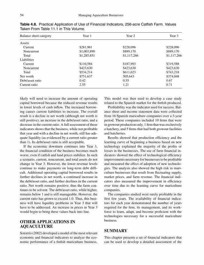
P1: SFK/UKS P2: SFK



Table 4.8. Practical Application of Use of Financial Indicators, 256-acre Catfish Farm. ValuesTaken From Table 11.1 in This Volume.

Balance sheet category Year 1 Year 2 Year 3

AssetsCurrent $281,961 $228,096 $228,096Noncurrent $1,003,890 $889,170 $889,170Total $1,285,851 $1,117,266 $1,117,266

LiabilitiesCurrent $110,584 $187,993 $319,588Noncurrent $423,630 $423,630 $423,630Total $534,214 $611,623 $743,218

Net worth $751,637 505,643 $374,048Debt/asset ratio 0.42 0.55 0.67Current ratio 2.55 1.21 0.71

likely will need to increase the amount of operatingcapital borrowed because the reduced revenue resultsin lower levels of cash inflow. The increased borrow-ing causes current liabilities to increase. The overallresult is a decline in net worth (although net worth isstill positive), an increase in the debt/asset ratio, and adecrease in the current ratio. A full assessment of theseindicators shows that the business, while not profitablethat year and with a decline in net worth, still has ade-quate liquidity (as evidenced by a current ratio greaterthan 1). Its debt/asset ratio is still acceptable.

If the economic downturn continues into Year 3,the financial condition of the business becomes muchworse, even if catfish and land prices stabilize. In sucha scenario, current, noncurrent, and total assets do notchange in Year 3. However, the lower revenue levelscontinue to make payments on long-term debt diffi-cult. Additional operating capital borrowed results infurther declines in net worth, a continued increase inthe debt/asset ratio, and further declines in the currentratio. Net worth remains positive; thus the farm con-tinues to be solvent. The debt/asset ratio, while higher,remains below 1 and is still manageable. However, thecurrent ratio has grown to exceed 1.0. Thus, this busi-ness will have liquidity problems in Year 3 that willhave to be addressed. An increase in prices in Year 3would begin to bring these values back into line.


Sotorrıo (2002) developed a model of the most relevanteconomic and financial indicators to analyze the eco-nomic performance of a finfish mariculture business.

This model was then used to develop a case studyrelated to the Spanish market for the finfish produced.

Profitability was the indicator used for success. Bal-ance sheet and income statement data were collectedfrom 16 Spanish mariculture companies over a 3-yearperiod. These companies included 10 firms that werein growout production only, 1 firm that was exclusivelya hatchery, and 5 firms that had both growout facilitiesand hatcheries.

Results showed that production efficiency and thelearning curve of beginning a business based on newtechnology explained the majority of the profits orlosses in the businesses. The use of farm financial in-dicators showed the effect of technological efficiencyimprovements necessary for businesses to be profitableand measured the effect of adoption of new technolo-gies. The analysis also showed the high risk in mari-culture businesses that result from fluctuating supply,market prices, and farm revenue. The financial indi-cators also measured the improvement in efficiencyover time due to the learning curve for mariculturecompanies.

The companies studied were rarely profitable in thefirst few years. The availability of financial indica-tors for each year demonstrated the number of yearsrequired for the firm, its management, and its work-force to learn, adapt, and become proficient with thetechnologies necessary for a successful mariculturebusiness.

SUMMARY

This chapter presents a set of financial indicators thatcan be used to develop a detailed assessment of the

P1: SFK/UKS P2: SFK



performance of an aquaculture business. These indi-cators can be tedious to calculate and can also be con-fusing due to the number of different possible indica-tors. Yet, the size of many aquaculture businesses andthe amount of capital invested requires the managerto pay this level of attention to detailed analysis to besuccessful.

REVIEW QUESTIONS

1. Describe some of the most critical indicators ofproduction efficiency on an aquaculture farm.

2. Give three examples of indicators of input use effi-ciency and explain what each indicator measures.

3. Explain the difference between the ROA and theROE.

4. Describe how to apportion net farm income amongcapital, labor, and management and what valuethese have for management decisions.

5. Define solvency and explain its importance in fi-nancial analysis of aquaculture businesses.

6. Explain how changes in net worth should be usedto assess the financial condition of the business.

7. Contrast the debt/asset, equity/asset, and debt/ eq-uity ratios in terms of how they are calculated,how they are related, and what they indicate aboutthe aquaculture business.

8. Explain the importance of liquidity, describe threecommon methods to calculate liquidity, and ex-plain how each is interpreted.

9. What two financial statements can be used to eval-uate liquidity?

10. Describe two measures of repayment capacity.

REFERENCE

Sotorrıo, LL. 2002. Economic analysis of finfish mari-culture operations in Spain. Aquaculture Economicsand Management 6(1/2):65–79.

P1: SFK/UKS P2: SFK


P1: SFK/UKS P2: SFK


5Financing an Aquaculture Business

INTRODUCTION

Financing has been difficult for many aquaculture busi-nesses. This is primarily because aquaculture has beenconsidered a risky enterprise by many lenders. As aconsequence, interest rates on aquaculture loans havetended to be higher and terms of lending more strin-gent than for other types of loans. Conventional loansmay not be available at all for aquaculture businessesin some areas because lenders are too uncomfortablewith the business. A lender who does not understandthe production system, expected patterns of cash flowand price fluctuations will tend to be unwilling to ex-tend credit without a substantial level of financial se-curity to back up the loan.

This chapter discusses lending to aquaculture busi-nesses from the lender’s perspective, financial char-acteristics of borrowers and their behavior, credit re-serves, and credit capacity. Credit problems faced bysmall-scale aquaculture growers in developing coun-tries are also discussed. Chapter 14 presents informa-tion related to the mechanics of structuring loan pay-ments and discusses various types of loans and termsof lending.

Lending From the Bankers’Perspective

A bank is a private, commercial business with the goalof making a profit, just as an aquaculture business isdeveloped to make a profit. Banks approve loans toearn money from the interest charged. Interest is the“cost” of money to the borrower, but to the banker, theinterest rate is the “price” charged for the resource andservice provided by making capital available to otherbusinesses.

A bank obtains its profit over time as loans are paidback. The risk that the capital loaned out will not bereturned in its entirety constitutes a substantial riskfor the bank. A loan made to a risky business ven-ture will put the bank’s capital at risk also. Successfulbanks must put safeguards in place to minimize therisk of losing their capital. As a bank’s capital is re-duced by defaulted loans, the bank must draw upon itsreserves to maintain adequate liquidity. Without ade-quate capital reserves, the bank will fail and go out ofbusiness.

While the borrower benefits directly from any profitsobtained as a result of a loan, the lender does not. Thelender’s “profit” or returns are restricted to the interestpayments that are specified in the loan agreement. Thelender may benefit indirectly if the borrower’s businessgrows over time and its financing needs increase.

A Bank’s Business

Banks, like aquaculture farms, are businesses. Theyoperate for the purpose of generating profits to dis-tribute to their stockholders. Just as aquaculture farmbusinesses must account for risk, a bank business mustalso manage its business with respect to risk and liq-uidity.

Banks manage their capital resources (financial as-sets) in a number of different ways. First, banks mustmaintain a certain amount of capital in the form ofreserves. Secondly, capital is used to extend loans andto make investments. Additional capital is used to pro-vide services to its customers. Capital is also usedto pay dividends to stockholders and to pay incometaxes.

A bank’s loan portfolio can include a variety of typesof loans that may include commercial and industrial,agricultural, consumer, and real estate loans. Extend-ing loans results in greater profits, but lending alsoentails the greatest risk and reduces bank liquidity.


57

P1: SFK/UKS P2: SFK



Commercial banks must maintain a high degree ofliquidity in their asset structure. The loan portfolio istypically a major part of the asset structure of a bank.

EQUITY VERSUS DEBT

Not all capital for aquaculture businesses is obtainedfrom traditional lenders. Some agricultural operationsalso obtain capital in the form of outside equity. Equitycapital in agriculture has been obtained mostly fromretained earnings from the business, inheritances, andgifts. However, equity capital can be obtained in otherways. Partnerships, joint ventures, and family corpora-tions can be used to pool capital and provide a sourceof equity capital. Some equity capital can be availablefrom outside investors seeking to shelter high nonfarmincome from taxes.

Limited partnerships have been used as a way to pro-vide equity capital in some types of agricultural oper-ations, particularly cattle feedlot operations. However,such a source of capital can be withdrawn as easily as itis made available. In such an arrangement, the investorincurs risk associated with limited opportunities to sellout their financial interest in the farm business.

Because new equity must come from either the cur-rent owners or new investors, it is important to under-stand the costs involved. Current owners can provideequity capital through investing the earnings or profitsfrom the business back into the business or by in-vesting capital earned through other sources. Outsideequity capital can be obtained by adding partners tothe business.

Investing the profits from the business back intothe business also represents a cost to the business,despite the fact that there is no definite repaymentschedule. The cost of reinvesting retained earnings isa type of opportunity cost that has been referred toas the required rate of return to compensate for theinvestment options that are forfeited. In addition, ifthe risk associated with the aquaculture business isgreater than that of other investment opportunities, theopportunity cost is greater.

The cost of obtaining outside capital for the farm isrelated to the rate of return that would be necessary toattract it. In other words, the rate of return from theaquaculture business will need to exceed that of othertypes of investment opportunities to attract investors.

Equity capital frequently ends up being more expen-sive (after taxes) than debt capital. This is particularlyso when the cost of retained earnings is considered, asit should be in a complete analysis.

The costs of debt capital include the interest paidalong with any loan settlement costs. Loan settlementcosts can include points charged at the initiation of theloan, any transactions fees, fees for credit reports, andany insurance premiums that are required. This cost isthe difference between the funds that are received bythe borrower and the total funds used to close out theloan.

LENDER PREFERENCES

Different types of lenders will have different prefer-ences for various types of lending terms. High-riskloans are often less preferred and will deplete creditrapidly. High-risk loans frequently have low loan limitsto restrict the overall extent of losses. High manage-ment ability is also preferred by lenders. Highly skilledand experienced management increases the likelihoodof repaying loans in a timely manner.

Lenders tend to prefer loans that are self-liquidatingand that generate assets. Self-liquidating loans arethose for which the loan is paid off with the incomegenerated by the equipment or other uses of the capitalbefore the new piece of equipment wears out. Theseare considered to be loans with lower levels of risk. Ifthe loan matures earlier than can be paid from the in-come generated by the asset acquired by the capital,income from other sources may need to be used tomake the payments. Crop inputs such as fingerlingsand fertilizer typically mature when the foodfish aresold, but machinery and equipment may have loans thatmature sooner than the number of years over which thepiece of equipment will be used.

An asset-generating loan is one used to acquire cap-ital goods such as equipment, ponds, or land that resultin an increased value of assets in the aquaculture busi-ness. As the value of assets in the business increases,these assets can be used as collateral in the future.

Lenders consider loans that are both asset-generating and self-liquidating as most preferable.Those that are asset-generating but not self-liquidatingand those that are self-liquidating but do not generateassets are of medium preference by lenders. Thosethat are neither self-liquidating nor asset-generatingare not preferred by lenders and are much less likelyto be approved.

The lender may prefer a loan length that is shorterthan the economic life expectancy of the asset beingfinanced. On the other hand, the borrower might prefera longer length of the loan. Open discussion may benecessary to work out an acceptable loan agreement.

P1: SFK/UKS P2: SFK


Financing an Aquaculture Business 59

EXPECTATIONS OF BANKREGULATORS ON LENDINGPRACTICES

Banks are regulated in different manners and by differ-ent agencies depending upon the type of charter underwhich they operate. State-chartered banks are regu-lated by individual state banking commissions whereasfederally chartered banks are regulated by the FederalDeposit Insurance Corporation. Regulatory agenciesand the laws that govern them were created to ensure asafe and stable financial sector. Bank regulations spec-ify the extent of capital reserves, lending limits, anddeposit insurance that each bank must maintain. Therelevant regulatory agencies have authority to auditand conduct examinations of banks to ensure compli-ance with all relevant regulations. Those who conductthe audits are termed as examiners. Bank examinershave guidelines for the adequacy of capital, liquidity,and asset quality that are used each time the examinerinspects the bank.

Each bank is required to maintain certain levels ofreserves to ensure that the bank is operating with ade-quate liquidity. While the level of reserves varies due totheir charter and the relevant regulations, required re-serves frequently are approximately 3% of transactionbalances. The Federal Deposit Insurance CorporationImprovement Act of 1991 set standards for the ade-quacy of a bank’s capital. This guideline differentiatesbetween banks with different types of asset risk anddivides a bank’s capital into different categories. Re-quired capital for each bank is based on percentagesfor each type of capital as well as total capital.

When a loan is not viable and the lender is forced todeclare bankruptcy, the bank risks losing some portionof the principal that had been loaned out. Banks mustcover this portion by transferring reserves to cover theloss. When reserves are transferred, the dollar amountthat the bank can lend is also reduced. Thus, absorbingloan losses reduces the volume of business that can beconducted by the bank because it loses reserves as aconsequence.

The amount that a bank can lend to any one individ-ual varies with the amount of equity capital owned bythe bank. Banks with national charters have loan lim-its that must be less than 15% of the bank’s net worthunless the loan is secured by collateral that can be mar-keted readily. Loan limits of state-chartered banks arevariable based on state regulations.

Many agricultural banks are small, rural banks.Their small size is reflected in lower amounts of re-serves. Thus, agricultural banks frequently find it more

difficult to grant large agricultural loans. Some smallagricultural banks develop relationships with otherlenders to meet the lending requirements of larger cus-tomers.

FINANCIAL CHARACTERISTICS OFBORROWERS AND SAVERS

The need to borrow capital is related to the level andrate of savings of the farm owner and manager. Dif-ferent reasons exist for savings. Seasons of the year inwhich farm sales are prevalent result in positive cashflows that can be a source of savings. Savings can beused for investments that produce an adequate finan-cial yield at an acceptable level of risk. The decisionto save earnings from the farm can be used to developcash reserves that will be available to the farm businessduring times of adverse conditions.

Some individuals who save do so to accumulatewealth. Accumulated wealth can be used to generatehigher earnings in later years.

Borrowing by farmers has increased over time asthe total investment per farm has increased. In partic-ular, investment in farm cooperatives, real estate, andequipment has increased substantially. Farmers haveincreasingly turned to debt to finance business growth.Overall, the size of the loans and the size of the repay-ments required for farmers have increased over time.

For farmers to borrow funds, individuals who savefunds must be willing to allow them to be used forfarm loans. Financial intermediaries, such as tradi-tional lenders and federal agencies have developedprograms to provide some guarantees that reduce therisk exposure of savers’ investment funds to the risksinherent in farm lending. These guarantees includethose from the Federal Deposit Insurance Corpora-tion, the Federal Housing Administration, Small Busi-ness Administration, Veterans Administration loans,and the Farm Credit System. Financial intermediariescan spread the risk of loans over broader areas andnumbers of borrowers. The federal Farm Credit Sys-tem, for example, can sell securities in national finan-cial markets.

SOURCES OF LOAN FUNDS

There are a number of different sources of loan fundsthat can be used by aquaculture businesses. The majorsource of loan funds for agriculture is from commer-cial banks. Many of those are rural agricultural banks.Commercial banks are a major source of operating cap-ital as well as some real estate loans. Smaller banks,

P1: SFK/UKS P2: SFK



without the reserves that enable them to grant loans tolarger farms, can develop an arrangement for a corre-spondent bank to supply loans to larger customers.

The Farm Credit System has been a major source ofcapital for aquaculture in the United States. It obtainsfunds through the sale of bonds and notes. Four re-gional Farm Credit Banks and one Agricultural CreditBank provide loan funds to local associations. Theseloans can be used for noncurrent loans for livestock,machinery, buildings, and land. Some operating capitalloans are also made by the Farm Credit System.

The Farm Service Agency of the U.S. Departmentof Agriculture has been an important player in creditfor U.S. aquaculture by providing guarantees to com-mercial banks for agricultural loans. These guaranteeshave encouraged private banks to grant loans to fishfarmers. With a guaranteed loan, the FSA guaranteesup to 95% repayment if the borrower defaults on theloan.

Farm supply companies have also been a source ofoperating capital for fish farms in the United States.Some of these types of operating loans are tied topurchases of feed or to contracts to supply fish to aprocessing plant.

ESTABLISHING AND DEVELOPINGCREDIT

Why should a lender approve a loan application? Abank is not a charitable organization, but a for-profitbusiness. The burden to prove that the borrower willrepay the loan with interest in a timely manner is on theprospective borrower. Individuals that have a demon-strated history of timely repayment of loans will likelyfind it easier to obtain credit, borrow greater amountsof capital, and perhaps obtain more favorable terms oflending.

Key factors involved in establishing and developingcredit include the character of the individual, demon-strated management ability, financial position as evi-denced by the balance sheet, repayment capacity, thepurpose of the loan, and the amount of collateral avail-able to secure the loan. Banks weight these various fac-tors differently, but most banks consider all the abovefactors to one degree or another.

The personal integrity of the prospective borrower isan important characteristic. A reputation as an honestbusinessperson will help to convince the lender thatthe estimated values in the business loan proposal areaccurate.

Aquaculture businesses are management-intensiveand require skilled management. Clear evidence ofmanagement experience of either the owner or thehired manager is key to a successful loan application.Established farmers will have records to demonstratetheir management expertise.

The balance sheet indicates the financial strengthor weakness of the borrower. Some lenders view thebalance sheet as the most important financial state-ment because it shows the degree of leveraging ofthe business and the availability of collateral to use tosecure new loans. The financial position of the businessalso indicates whether the net worth of the business hasgrown over time. Steady growth of the business reflectspositively on the management and financial position ofthe business.

The lender is concerned primarily with repaymentof the loan. Thus, the borrower must demonstrate ad-equate liquidity and a favorable cash position. A de-tailed cash flow budget will demonstrate clearly theability of the business to repay new loans that are pro-posed.

Self-liquidating loans frequently are financed moreeasily than other types of loans. This is because the loancan be repaid from the sale of the crop or livestockfinanced by the loan. Loans used to acquire capitalassets may require additional collateral because theseassets are not typically sold themselves to generaterevenue.

Land is one of the more frequently used types ofcollateral for aquaculture businesses. Buildings, equip-ment, and, occasionally inventory of livestock can alsobe used as collateral. Award of the loan should bebased on clear evidence that the loan payments can bemade from revenue from the farm rather than collat-eral. However, lenders ask for collateral to cover therisk of unexpected adverse conditions that may resultin default of the loan. In aquaculture, personal assetssuch as a home have been used as collateral.

Borrowing Behavior

The capacity to borrow funds can be turned into bor-rowing behavior or it can be held as a reserve for futureborrowing as needed. The decision as to whether toborrow the maximum that a lender’s criteria will allowor to borrow some lower amount and reserve the ca-pacity to borrow for some other purpose in the futureshould be based on the relative profitability of the al-ternatives. The level that constitutes the maximum an

P1: SFK/UKS P2: SFK



individual can borrow is based on the credit worthinessof the borrower.

The value to an individual of holding credit in re-serve rather than borrowing the maximum will varywith the level of risk aversion of the individual and thestrategies undertaken on the farm to manage risk (seeChapter 16 for a more complete discussion of risk andChapter 8 for more discussion on managing risk onaquaculture farms).

Credit Capacity and Credit Reserves

Credit reserves refer to additional borrowing that afarmer likely would be able to obtain if desired. Atany point in time, one or more lenders may be willingto loan additional funds to a firm or individual bor-rower to finance transactions. Credit reserves exist onfarms that have not borrowed the maximum amountcalculated by the lender when determining the creditworthiness of the individual. The credit worthiness willvary with the profitability of the business, the individ-ual’s balance sheet, net worth, and assets available foruse as collateral, as well as the individual’s demon-strated management skill. The maximum amount thatcan be borrowed will also fluctuate with overall trendsof national and international economies.

The availability of credit reserves is particularly im-portant when the farm faces adverse conditions. Eco-nomic downturns may result in lower prices and rev-enue for the farm or conditions may occur that resultin increases in prices of key inputs such as feed. Dur-ing these times of economic adversity, the cash flowof the farm business may suffer and credit reservesmay be accessed to increase borrowing of operatingcapital. Alternatively, credit reserves may be used torefinance loans, defer loan payments, or carry over orextend loan maturity dates. Credit reserves can play animportant role in managing the debt on the farm, par-ticularly during times of adverse financial conditions.

Holding credit reserves means that the farm is notusing all its potential for borrowing. Credit is an excel-lent source of liquidity and, if holding credit reservesresults in levels of liquidity that are lower than opti-mal, the wise decision may be to increase liquidity bytaking advantage of the credit reserves and borrowingadditional funds. However, maintaining only low lev-els of credit reserves increases financial risk becausethere is little to draw upon during difficult economictimes. Moreover, greater control of the business is ex-ercised by lenders when the business has a high degreeof debt.

Determinants of Credit

The availability of credit is a complex phenomenonthat is influenced by characteristics of the particularlender as well as trends in financial markets. Lendersseek profit and prefer higher rates of return earned overa shorter period because risks typically are less andmore clear over shorter time periods. Lenders must alsomaintain a high degree of liquidity in their business.This may result in banks preferring shorter loans thatmay be less than the economic life of the asset.

Current trends in the macroeconomy will influencethe availability of credit. Current national fiscal andmonetary policies and international trade conditionswill affect credit conditions. The financial condition ofthe marketplace will affect the availability and the costof credit. Monetary and fiscal policies, inflation rates,the overall national money supply, and the aggregatenational economic performance will have an effect onthe availability of credit.

Financial conditions of the individual bank will af-fect how readily it will make loan funds available. Theprofitability of the bank, its loan loss rate, the rate ofloan delinquency, and its size will all affect the amountof capital to be loaned. Each bank will also be affectedby its size, costs, and the particular legal and regula-tory environment within which it operates. The bank’spersonnel and board of directors will have an impacton the policies established by each bank.

Finally, financial conditions of the borrower’s busi-ness will affect the extent to which loan funds will bedirected toward it. Overall profitability of the indus-try, effects of international trade conditions, key inputprice trends, and other factors will affect the repaymentcapacity of the industry. The aggregate profit prospectsfor farm commodities as a whole, changes in the valueof farmland and resources, international trade condi-tions that specifically affect the borrower’s business,and how government farm programs are expected toaffect the business will impact the availability of credit.

Credit Evaluation

Lenders evaluate the credit level of prospective bor-rowers in various ways. Some are mostly subjectiveand informal while others have more formal creditscoring methods. The purpose of a credit evaluationis to identify the borrower’s credit worthiness and bydoing so to measure the credit risk. Credit evaluationis used to compare good and poor credit risks to de-cide which loans to approve and which to reject. In

P1: SFK/UKS P2: SFK



some cases, interest rates charged may depend uponthe credit evaluation or if any specific monitoring sys-tem needs to be put in place.

The credit worthiness of the individual borrower isthe lender’s evaluation of the profitability and the risksassociated with lending to an individual borrower. Theevaluation of a borrower’s credit worthiness is basedon the evidence presented by the borrower to assurethe lender that lending risks will be minimal and thatdebt servicing will meet the terms of the loan contract.

Credit scoring has been used commonly in consumerlending. To develop a credit score, key characteristicsare identified and then assigned a weighting factor.The weighted averages of these characteristics are thensummed to generate a credit score. The credit charac-teristics frequently include the estimated profitabilityof the business, the projected liquidity of the business(current ratio), solvency of the business (debt/equityratio), the collateral position (ratio of the maximumloan balance to assets pledged as security), and loanrepayment capacity (debt-servicing ratio). The creditscore will change over time as the values of each char-acteristic change for the business. The assets (bothquantity and quality) available for security for the loan,repayment and income expectations, and other finan-cial management practices of the borrower will affectone’s credit profile and score.

SOLVENCY

Solvency of a business is a key measure of the finan-cial strength or weakness of the business. A solventbusiness is one that, if the business were to be sold, thevalue of the assets sold would exceed the value of theliabilities, and all debts would be paid in full.

The overall financial structure of the business affectsthe level of financial risk involved. There are variousmeasures available to monitor the use of capital andcredit in the farm business. Chapter 4 presents detailsof how to calculate a variety of different financial ratiosthat provide measures of the solvency of the business.One of the more important measures is the debt toequity ratio that is calculated from the balance sheet.Coverage ratios, such as the interest coverage ratio,are calculated from the income statement that relatesthe returns to assets from the business to the debtobligations.

FINANCING CURRENT ASSETS

The majority of current assets in aquaculture are op-erating inputs. These inputs of feed, fuel, labor, etc.,

typically are not carried over into the next year. Operat-ing inputs typically do not constitute collateral becausethey are not easily sold. Thus, the borrower frequentlymust use other sources of collateral for operating in-puts. The one exception in many forms of agricul-ture is that of livestock. Inventories of feeder livestockcan be used as collateral for operating loans; however,swimming inventory of fish is rarely considered an ac-ceptable source of collateral for aquaculture operatingloans.

Financing current assets is a high-priority type offinancing for a fish farmer. It is essential to have ad-equate capital to feed fish, and the capital must beapproved and in hand when the feeding season is athand. The most critical terms of lending for an op-erating loan are the loan maturity and the repaymentschedule. Collateral and interest rates must also beplanned carefully.

To be a self-liquidating loan, the operating loan willneed to be repaid from sales of the products that werefinanced from the operating loan. Payments on oper-ating loans typically are made with each shipment offish delivered to the processing plant.

FINANCING DEPRECIABLE ASSETS

Depreciable assets primarily include equipment suchas aerators, vehicles, feed wagons, and other types ofequipment used on fish farms. Pieces of equipment areused over a number of years and are replaced either asthey wear out or as new technology becomes available.Typically, replacement of equipment can be plannedover a period of time to set up the financing in a waythat the payments are scheduled when cash is readilyavailable.

For a loan to acquire a depreciable asset to be self-liquidating, the terms of lending (loan maturity andrepayment schedule) should match the revenue thatis produced by the asset. Some industries scheduleequipment loans to match the depreciation of the as-sets. Most equipment loans have a loan maturity of5–7 years.

FINANCING FIXED ASSETS

Fixed assets in aquaculture include land, ponds, wells,office buildings, hatcheries, and grading sheds. Ofthese, land is the only nondepreciable asset. Thus,land is not used up in the production process. Realestate loans can have maturities that range from 15 to30 years. Payments of farm mortgages and other realestate loans are fixed payments. Fish farms that are

P1: SFK/UKS P2: SFK



highly leveraged will have high levels of fixed loanpayments that must be met. The need to make thesepayments reduces management flexibility, particularlyduring times when fish prices are low, or feed pricesare high. During these times, it may be more profitableto reduce feeding and stocking rates; however, farmsthat are highly leveraged will need to continue to stockand feed at high rates to produce yields that will enablethem to continue to meet the fixed loan repayments.

SOURCES FOR LOAN REPAYMENT

Real estate loans typically are repaid from retainedearnings of the aquaculture business. A variety ofsources can be drawn upon as sources of capital forloan repayment. Ideally, sources of funds for an operat-ing loan would come from cash that has been set asideto pay operating expenses. Equipment loans would bepaid from cash set aside to account for depreciationwhile retained earnings (profits less income taxes andfamily withdrawals) frequently are used as the majorsource of funds to repay real estate loans.

CREDIT PROBLEMS FACED BYSMALL-SCALE AQUACULTUREGROWERS IN DEVELOPINGCOUNTRIES

Small-scale aquaculture growers in developing coun-tries face special problems related to acquiring suf-ficient credit to finance their businesses. Investmentcapital generally is a major obstacle to developmentof aquaculture businesses in developing countries(Hishamunda and Manning 2002). There are numer-ous factors that exacerbate the credit problems faced bysmall-scale aquaculture growers in developing coun-tries.

Lack of collateral typically is one of the first obsta-cles to gaining access to credit. Small-scale growersfrequently lack the level and types of assets consid-ered as acceptable collateral by banks. Land, homes,and other types of assets are preferred sources of collat-eral that often are not available for use by small-scalegrowers.

Many developing countries contend with exces-sively high interest rates on loans. Interest rates of40–60% are not uncommon. Businesses that can suc-cessfully pay off loans at such high rates are very rare.The high interest rates can stem from unstable nationaleconomies that result in a risky financial market or re-strictive monetary policies and supply of money that

result in very high costs of capital. High rates of defaulton loans also put upward pressure on interest rates.

Many small-scale growers also lack the knowledgeand skill required to prepare a proper business planand loan proposal. Required information may not bereadily available and the expertise to prepare financialstatements properly may not be available.

Group lending to small-scale growers has proven tobe an innovative approach to overcome some of theirobstacles. The Grameen Bank pioneered these effortsin the mid-1970s in Bangladesh (Grameen 2001). Itloans to the poorest of the poor, to borrowers withoutcollateral. By 2001, the Grameen Bank had grown to2.38 million borrowers lending $31 million a weekin very small loans, with a repayment rate of 90%.The approach is based on peer pressure, small weeklyrepayments, and personal contact with borrowers. Theconcept has spread to 58 countries.

In addition to group lending, village banks and sol-idarity groups have been used to counter the problemsof collateral. The village bank receives one loan thatis shared with all members. It must be repaid in fullbefore it receives another.

RECORD-KEEPING

The aquaculture farm business should keep recordsof each proposal for a loan and the financial state-ments used to acquire the loan. Once the loan is ob-tained, records should include the history of debt ser-vicing that includes each payment made, the amountof the payment made on the principal, and the amountpaid for interest. These records will assist the farmerwhen preparing other financial statements such as thebalance sheet, income statement, and the cash flowbudget.


This practical application is based on a 431-acre catfishfarm that is a startup farm that borrowed 65% of itsreal estate and equipment capital to enter the catfishbusiness. In doing so, the pro forma income statementshowed that the farm was profitable, but profit levelswere relatively low. There was substantial financialrisk generated by the low profit levels because anyadverse economic conditions such as unexpectedly lowprices or disease problems would result in losses. Thelosses would also create cash flow problems that wouldmake it difficult to meet debt-servicing requirements.

In consultation with extension personnel and re-viewing the latest research results, it became apparentthat this farm had entered business with too few

P1: SFK/UKS P2: SFK



aerators. Research had shown that by doubling theaeration capacity of the farm from 1 to 2 hp/acre totalyield of catfish would increase. This would result inincreased revenues and profits. The increased revenueswould further improve cash flow of the business andreduce the risk associated with meeting debt-servicingobligations.

Acquiring an additional 10-hp aerator for each of thefarm’s 43 ponds would require an additional equipmentloan of $150,500. To apply for the loan would requirean analysis of the financial structure and position ofthe business.

The 431-acre farm’s balance sheet showed adequate,although low, liquidity with a current ratio of 1.13(Table 5.1). Working capital was $21,275, low for this

Table 5.1. Catfish Farm Balance Sheet,431-acre Farm, End-of-Year.

Category Value


Cash on deposit $31,000Fish inventory $150,000Total current assets $181,000

2. Noncurrent assetsEquipment $606,035Ponds $602,538Wells $81,000Land 354,282Total noncurrent assets $1,643,855

3. Total assets $1,824,855

Liabilities4. Current liabilities

Payments on debt due and payableover next yearEquipment $80,914Real estate $78,811

Total current liabilities $159,7255. Noncurrent liabilities

Equipment loan $393,923Real estate loan $674,583Total noncurrent liabilities $1,068,506

6. Total liabilities $1,228,2317. Net worth $596,624

Current ratio (1/4) 1.13Working capital (1–4) $21,275Equity/asset ratio (7/3) 0.33Debt/asset ratio (6/3) 0.67Debt/equity ratio (6/7) 2.06Debt structure (4/6) 0.13

size of farm. However, the debt/asset ratio was 0.67and the debt/equity ratio was 2.06. The equity/assetratio was 0.33. The debt structure was 0.13, indicatingthat the majority of the debt was in the long-term debtassociated with the real estate and equipment loans. Inconclusion, the farm’s balance sheet does not show ad-equate equity to support additional borrowing. Long-term borrowing already shows levels that would bedeemed unacceptable to the lender. Increasing debt-servicing requirements would decrease working capi-tal and increase financial risk to unacceptable levels.

The owner of the farm has a relative who has beenin the catfish business for many years. This relativeconstructed his own ponds over the previous 20 yearsand has no outstanding debt related to its real estate.The relative’s farm also owns all the equipment on hisfarm. The equipment was financed with retained earn-ings from the farm business. Thus, the debt obligationsof the relative’s business are low. In conversations overthe difficulties of developing a fish farming businesswith high levels of debt financing, the two farmers de-cide to merge their farming businesses into one busi-ness. They believe that they will achieve economiesof scale and improve overall production efficiencies.However, both farms, once merged, will need to in-crease aeration levels to 2 hp/acre. This will require$301,000 in capital that the owners believe will needto come from debt capital.

Table 5.2 presents the revised balance sheet for thenow-merged farm business. The new equipment loanof $301,000 has been added to the noncurrent liabilitiesand the annual payment for the new loan has beenadded to current liabilities. Noncurrent assets have alsobeen increased by $301,000 to account for the newaerators that have been acquired.

The overall financial position of the merged busi-ness, even with the new equipment loan for the aera-tors, has improved considerably. The current ratio hasimproved to 1.63 and working capital has increasedto $140,448. These liquidity measures show a reduc-tion in financial risk associated with the business’ cashflow position. The equity/asset ratio has increased to0.60, the debt/asset ratio has decreased to 0.40, andthe debt/equity ratio has decreased to 0.67. The debtstructure shows little change; much of the debt still re-mains in longer-term debt. However, the liquidity hasimproved substantially and the longer-term financialindicators are within acceptable ranges. These rangeswill likely be viewed as acceptable levels of risk tothe lender. Thus, the merger has created a financialposition for the business that is likelier to result in

P1: SFK/UKS P2: SFK



Table 5.2. Catfish Farm Balance Sheet,862-acre Merged Farm, Including NewEquipment Loan to Expand Aeration Rates to2 hp/acre, End-of-Year.

Category Value


Cash on deposit $62,000Fish inventory $300,000Total current assets $362,000

2. Noncurrent assetsEquipment $1,513,070Ponds $1,205,076Wells $162,000Land 708,564Total noncurrent assets $3,588,710

3. Total assets $3,950,710

Liabilities4. Current liabilities

Payments on debt due and payableover next yearEquipment $142,741Real estate $78,811


Equipment loan $694,923Real estate loan $674,583Total noncurrent liabilities $1,369,506

6. Total liabilities $1,591,0587. Net worth $2,359,652

Current ratio (1/4) 1.63Working capital (1–4) $140,448Equity/asset ratio (7/3) 0.60Debt/asset ratio (6/3) 0.40Debt/equity ratio (6/7) 0.67Debt structure (4/6) 0.14

favorable consideration by a lender. The addition ofthe aerators should result in greater profits and rev-enue for the business.


Analysis of the financing requirements and repaymentfeasibility is vital to adequate planning for success-ful aquaculture businesses of all types. Pomeroy et al.(2004) analyzed the financial feasibility of aquacul-ture cage businesses for two species of grouper. Theanalysis showed that, overall, cage culture of grouper

is financially feasible. However, financing of the busi-nesses is likely to be difficult, particularly on a smallscale. This is because the capital required for the vari-ous stages of production (broodstock, hatchery, or ver-tically integrated systems) exceeds the borrowing ca-pacity of small-scale producers. Loans would likelybe necessary for growout production, particularly forsmall-scale farmers. However, the analysis of cash flowdemonstrated that the loans could be repaid within oneyear of production.

SUMMARY

This chapter has described lending primarily from theperspective of the lender. Commercial banks are for-profit companies that seek to provide capital to othersfor a fee (interest rate). Success in obtaining loans ishigher when the prospective borrower understands theperspective of the lender and requirements of the bank.Each bank is limited in the amount of loans that can bemade and in the size of individual loans. These limitsare related to the reserves maintained by the bank.Loan defaults require the banks to spend reserves tocover the losses, thus reducing the overall amount ofreserves and the amount of loans that can be madeagainst those reserves.

Banks use various methods to evaluate the creditworthiness and credit capacity of prospective borrow-ers. However, whether an individual bank uses a for-mal or more subjective process of evaluating credit,the potential profitability, the repayment capacity, theamount of assets available for use as collateral, themanagement expertise of the owner, and the owner’sprevious history in business will typically influencethe decision of whether to grant the loan.

Ideal loans are self-liquidating and asset-generating.Current, depreciable, and fixed assets have differentcharacteristics that require various adaptations to beself-liquidating. Moreover, limits imposed by bank ex-aminers on lenders may result in a lender encouragingborrowers to agree to lending terms that result in aloan that is not self-liquidating. Careful analysis is re-quired of the various alternatives associated not onlywith terms of lending, but with the type of lender, withdefinitions of credit capacity, and with the types ofassets to be financed.

REVIEW QUESTIONS

1. Contrast the difference in perspective of the lenderfrom that of the borrower.

P1: SFK/UKS P2: SFK



2. What is a self-liquidating loan? Provide an aqua-culture example.

3. What is an asset-generating loan? Provide an ex-ample from aquaculture.

4. Describe differences in characteristics of borrow-ers and savers.

5. What are credit capacity and credit reserves? De-scribe why these are important and under whatconditions they may vary.

6. List several determinants of credit.

7. Contrast several different types of major lenders toaquaculture in terms of their charters, limitationson lending, and how different types of lenders areregulated.

8. Contrast the differences in financing current, de-preciable, and fixed assets.

9. Describe several sources of loan repaymentfunds.

10. Describe how a new, young farmer can establishand develop credit for the business.

REFERENCES

Grameen. 2001. Grameen Fund. Found at http://www.grameen-info.org.

Hishamunda, Nathanael and Manning, Peter. 2002.Promotion of Sustainable Commercial Aquaculturein Sub-Saharan Africa. Volume 2. Investment andEconomic Feasibility. FAO Fisheries Technical Pa-per 408/2. FAO, Rome, Italy.

Pomeroy, Robert S., Agbayani, Romeo, DurayMaretta N., Toledo, Joebert D., and Quinitio,Gerald F. 2004. The financial feasibility of small-scale grouper aquaculture in the Philippines.Aquaculture Economics and Management 8(1/2):61–83.

P1: SFK/UKS P2: SFK


6Managing Cash Flow

INTRODUCTION

Cash flow problems result in more aquaculture busi-nesses’ failure than any other problems. Managingcash flow adequately and properly can make a dif-ference between the success and failure of a business.Liquidity is a financial concept that is linked closelywith cash flow. It refers to whether the business willhave the cash when needed to make its payments. Cashflow is a strong measure of liquidity.

A balance sheet can provide some limited indicationof liquidity in the farm business through calculating thecurrent ratio and level of working capital. However, thebalance sheet summarizes the values of all current as-sets and liabilities over the course of the year. If loanpayments are due in the early part of the year but fishare not sold until later in the year, there will be a liquid-ity problem that will not be evident from the balancesheet. An analysis that accounts explicitly for the tim-ing of receipt of cash and the expected payments isneeded. This chapter compares profitability with liq-uidity, identifies common types of cash flow problemsin aquaculture, discusses the use of cash flow state-ments and budgets to manage cash flow, and outlinesthe need for record-keeping.

LIQUIDITY

Farms that are profitable and viable businesses canalso have occasional cash flow problems. Adequateliquidity is essential to an aquaculture business becauseit is used as a source of cash to meet demands forcash payment, as a safety margin for adverse financialconditions, and as a source of capital for investmentin other alternatives. It measures the capacity of the

business to produce enough cash to make financialpayments when they are due. Positive cash flow isnecessary to meet operating expenses and to meet thecash needs of the farmer and his or her family.

PROFITABILITY VERSUS LIQUIDITY

Many business owners believe that the success of thebusiness is determined solely by its profitability. Suc-cessful businesses must be profitable, but inadequatecash flow can result in business failure. In fact, cashflow problems likely cause more severe financial prob-lems than overall issues of profitability.

Cash flow problems are problems of liquidity, notprofitability. Because cash flow measures the timingof receipt of revenue and of expenses, it is a primedeterminant of liquidity. However, cash flow budgetsinclude only cash items; noncash items such as de-preciation are not included. Cash flow budgets do notmeasure profitability.

COMMON SOURCES OF CASH FLOWPROBLEMS IN AQUACULTUREBUSINESSES

There are a number of different types of cash flow prob-lems that cause difficulty for aquaculture businesses.A common cause of liquidity problems involves thetiming of product sales. Aquaculture businesses withseasonal production, that is harvests occur in only oneperiod of the year, can face liquidity problems becauserevenue is not available throughout the year to coverexpenses when due. In a similar manner, the timing ofexpenditures can result in liquidity problems. Borrow-ing and loan payments, leverage and use of credit, andbusiness expansion also contribute to liquidity prob-lems. Moreover, farm planning can be hampered if theprojections of sales, expenditures, and payment sched-ules are forecasted incorrectly.


67

P1: SFK/UKS P2: SFK



Timing of Product Sales

Product sales that occur several months later than whenproduction expenses are incurred are a common sourceof cash flow problems. For example, a salmon crop isstocked at one point in time, typically, with one size offish. The fish are fed, kept free of disease, and moni-tored until they reach market size, often 9–15 monthsafter stocking (Bjorndal 1990; Grisdale-Holland et al.2004). The salmon farm must pay all bills associatedwith feeding, disease control and treatment, and costof the smolts, labor, and other expenses, but does notreceive revenue until the salmon are sold. This createsa clear cash flow problem that must be accounted forwhen planning the farm business. Production expensesmust be covered for the time period until sales generaterevenue.

Timing of Expenditures

The timing of expenditures can also create cash flowproblems. If a shrimp farm is planning to purchasenew aerators across the farm and prepares to make thepurchase at the beginning of a production cycle, theinvestment will result in a substantial outlay of cash atthe beginning of the production cycle, before shrimphave been produced and sold. Thus, there is no cashrevenue to match the cash outlay at that time of the year.If shrimp prices fall or feed prices increase, the farmmay no longer have a surplus from the previous yearto cover these adverse conditions because the surplusfunds were spent on the new aerators. Cash flow wouldbe improved by waiting to purchase the new aeratorsuntil the end of the production cycle, using revenuefrom shrimp sales.

Borrowing and Loan Payments

The characteristics and terms of loans on the farmcan have a strong effect on liquidity. The interestrates charged and the terms of payment (such as thelength of the loan) will affect the amount of the pe-riodic payment. Longer-term loans will have lowerpayments while shorter-term loans will have higherpayments. Restructuring debt can be used to improveliquidity by reducing the annual payment by extend-ing the length of the loan. However, restructured loanswill result in greater total interest paid over the lifeof the loan. Serious liquidity problems may requirerestructuring of loans, but this must be approachedcarefully.

The structure of the debt in the business refers tohow the debt is apportioned among short- and long-term loans. A high percentage of debt in short-termcurrent liabilities can be another cause of liquidityproblems. Refinancing can be a way to move the debtto longer term by amortizing the repayment over alonger period. The general rule for structuring loans isthat the repayment terms should match the useful lifeof the assets. For example, if a piece of equipment isexpected to last for 7 years, then the loan should bestructured to be repaid within 7 years.

Scheduled debt repayments can result in cash flowproblems. If payments on major loans, such as the realestate or equipment loans on the farm, are scheduledto be paid in the early part of the production season,cash flow problems may result. Cash flow is improvedby scheduling payments on loans to coincide with thetime of the year that is likeliest to have product salesthat generate revenue at the time the payments aredue. A repayment schedule that matches the timing ofrevenue and cash flow in the business can also reduceinterest expenses.

Leverage and Use of Credit

The financial risk of increased borrowing can result inliquidity and cash flow problems. Financial analystsoften talk about the trade-off between leverage andliquidity. The term leverage refers to the proportionof borrowed to equity capital. The higher the degreeof borrowed capital relative to the amount of capitalowned by the farm, the more highly leveraged thebusiness. Thus, leverage increases with the debt/assetratio.

Greater amounts of borrowing can deplete creditreserves. Credit reserves are one of the managementalternatives that can be used to prepare and plan foradverse cash deficits. Reductions in the amount ofcredit reserves reduce the business’ ability to withstanddownside risks. Increased borrowing also increases therepayment obligations in the future.

Business Expansion

Liquidity is important as a source of funds to takeadvantage of new investment opportunities. This mayinclude having capital to purchase additional land asit is put on the market, purchasing equipment at goodprices at auctions and farm sales, or funds to use as ahedge against adverse commodity prices in the mar-ketplace.

P1: SFK/UKS P2: SFK


Managing Cash Flow 69

Business expansion can result in cash flow and liq-uidity problems. For example, the farm may decideto add a hatchery to the farm because careful analy-sis has shown that vertically integrating the food fishgrowout operation with a hatchery and fingerling en-terprise will result in greater profits. The hatchery willrequire a new building, new ponds, and development ofbroodstock for spawning. Selecting broodstock fromcurrent stocks of fish may decrease the weight of fishavailable to be sold. Putting ponds into fingerling pro-duction reduces the acreage of water available for foodfish growout. Construction of the hatchery buildingand the ponds also requires cash outlays. The combi-nation of the reduced revenue from diverting fish tobroodstock and reduced acreage and the cash outlaysto construct the hatchery building may result in a tem-porary cash deficit. Over time, as the new ponds arebuilt and stocks of fish are built back up to former lev-els, the cash deficit will disappear and the increasedprofits will be realized.

Incorrect Anticipation and OverlyOptimistic Estimation of Costs,Yields, and Revenues

The accuracy of cash flow projections and budgetswill depend on the accuracy of the yields, prices, andcosts used to make the projections. The farm may baseyields on historical farm records. However, in anygiven year, disease problems, adverse weather con-ditions, or other unanticipated events may result inlower-than-anticipated yields. If yields achieved on thefarm are less than those anticipated and projected, therevenues projected will also be less than anticipatedand cash flow problems will likely result.

Fish prices are determined in the market and are out-side the control of the majority of aquaculture produc-ers. While close attention on price trends and cycleswill generally result in more accurate estimation ofprices, there are many forces that can result in unantic-ipated price changes. Lower prices received, as com-pared to those projected, will result in lower revenuethan projected with cash flow deficits and problemslikely resulting.

It can be difficult for many farmers to be disciplinedwhile forecasting prices and expenditures. The temp-tation is strong to be overly optimistic about prices,yields, and costs. One method to guard against mis-leading estimates is to have a frank and objectiveassessment of cash flow projections developed by athird-party individual. An outside analyst can often be

relied upon to inject some realism into the projections.Long-term datasets of prices and yields can also behelpful to maintain price and cost projections withinrealistic ranges.

Nonfarm Factors

Many farms are managed as a family operation withfamily expenses and obligations mixed in with thefarm’s expenses and obligations. If the farm familyhas a sudden increase in medical expenses or tuitionexpenses for college, these expenses can create a cashdeficit that spills over into the farm business.

STATEMENT OF CASH FLOWS

The statement of cash flows summarizes the actualcash inflow and outflow of the farm business overthe course of the production year. It presents an as-sessment of the cash position for each month of thebusiness. Thus, the statement of cash flows calculatesthe liquidity for each month. This statement should beprepared over the same fiscal year as the balance sheetand the income statement.

Table 6.1 illustrates the format of a statement ofcash flows. Cash farm income and expenses are sum-marized in the first section (Cash flows from operatingactivities). The second section (Cash flows from in-vestment activities) includes any investment revenueand expenses. The third section summarizes cash ob-tained from loans and the cash outflows from debt-servicing and repayment expenses. The fourth section(Cash flows from nonfarm activities) is for cash inflowand outflow from nonfarm items, while the final sec-tion balances the cash on hand. The cash flow statementdoes not include any noncash items. Noncash items areimportant in the determination of profitability and networth, but are not included in a statement of cash flowsbecause they are not cash items.

The example of a statement of cash flows in Table6.1 is for a farm that has no nonfarm revenues orexpenses. This farm received $604,800 in revenuefrom sale of fish and paid $564,433 for farm operatingexpenses. Net cash from operating activities was$40,367. The farm did not purchase or sell anybroodstock, equipment, or land. Cash obtained fromfinancing activities provided $173,650 from anoperating loan. Principal payments on longer-termdebt were $98,058. When the principal payments ofthe operating loan were included, the net change incash was negative, at −$57,692. Thus, this farm does

P1: SFK/UKS P2: SFK



Table 6.1. End-of-Year Statement of Cash Flows with 25%Market-Sized Fish Off-Flavor.

Item Total

Cash flows from operating activitiesCash received from farm operations $604,800Cash paid for farm operating expenses $564,433

Net cash provided by operating activities $40,367Cash flows from investment activities

Cash received from sales of:Broodstock 0Equipment 0Real estate 0

Cash paid to purchase:Broodstock 0Equipment 0Real estate 0

Net cash provided by investing activities 0Cash flows from financing activities

Operating loan received $173,650Term principal payments $98,058Operating debt principal payments $173,651

Net cash from financing activities −$98,059Cash flows from nonfarm activities

Cash received from nonfarm income 0Cash paid for nonfarm expenses 0Cash withdrawals for family living 0

Net change in cash −$57,692

not have adequate liquidity to pay off its operatingloan in full over this time period.

The operating line of credit can be determined andmonitored from the statement of cash flows. Its pur-pose is to be certain that the business has adequate liq-uidity in the months expected to result in cash deficits.An operating line of credit is designed to provide cashin months of cash deficits, and to repay deficits inmonths of cash surpluses.

The statement of cash flows indicates the amount ofthe operating line of credit required for each month.The statement of cash flows also shows the amount ofoutstanding operating capital debt for each month ofthe year. Increasing amounts of operating capital debtindicate increasing problems of liquidity. A preferableposition is for the amount of operating capital out-standing to decrease throughout the year, ideally, tozero. A feasible business is one in which adequatecash surpluses exist during enough months to pay offthe operating capital debt accumulated during monthsof cash deficits. If the outstanding operating capital

does not decrease throughout the year, there is a liq-uidity problem and there is likely a shortage of workingcapital.

MANAGEMENT ALTERNATIVESAND PLANNING STRATEGIES TOOVERCOME CASH FLOWPROBLEMS

The first step to managing and planning to avoid orovercome cash flow problems is to monitor and controlcash flow from the beginning. This requires planning,organizing, directing, and controlling the cash flow ofthe business. The last step, control, is to implement theactions that are necessary to be certain that goals andobjectives of the overall business plan are met.

This process involves establishing some initial per-formance standards. The business performance mustthen be compared against the standards and correctionsmade as necessary.

P1: SFK/UKS P2: SFK



Monitoring Cash Flows

Table 6.2 presents a sample of a form that could be usedto monitor cash flow for the aquaculture business. Thetotal amount of cash flow projected is entered into thefirst column. The amount budgeted up to the date thereport is prepared is entered in the next column, whilethe actual cash flow to date is entered in the third col-umn. Ideally, this report is prepared on a monthly basisfor frequent monitoring of the cash flow situation. Ifthe owner cannot schedule adequate time for monthlymonitoring, quarterly monitoring would still providesome degree of control throughout the year. Excessiveoutflows of cash will become readily apparent withfrequent monitoring, and a course of corrective actioncan be identified to avoid the development of more se-rious deficits. Monitoring cash flow only once every 6months, or once a year, is not adequate. The earlier thediagnosis of a potential problem, the sooner the cor-rective action and steps can be taken. Not monitoringcash flow can result in business failure.

Year-end estimates can be revised as necessary. Atthe end of the year, the past year’s cash flow perfor-mance can be used to develop a more realistic projec-tion for the upcoming year. Deviations in borrowings

and loan payments should be evaluated primarily basedon their effects on the ending cash balance.

Measures of Repayment Capacity

There are two measures of repayment capacity that arerecommended by the Farm Financial Standards Coun-cil (FFSC): (1) term debt and capital lease coverageratio, and (2) capital replacement and term debt repay-ment margin. The term debt and capital lease coverageratio is calculated with the following equation:

Term debt and capital lease coverage ratio

= cash available for term debt payments for

the past year/total of the term debt payments

due in the next year.

Term debt covers scheduled, amortized payments.The cash available for term debt payments is calculatedby adding the total nonfarm income, depreciation ex-pense, and interest paid on term debt and capital leasesto net farm income from operations and subtractingout withdrawals for family living and personal incometaxes. A value greater than 1.0 indicates adequate cashflow to meet the scheduled term debt payments. It is

Table 6.2. A Sample Form for Monitoring Cash Flows on Aquaculture Businesses in March.

Item Projected annual total Projected total to date Actual cash flow to date

Beginning cashPounds of catfish sold, lb 1,152,000 138,240 103,680

Receipts from catfish sold, $ 806,400 96,768 72,576Operating cash expenses

Feed 278,264 13,913 13,913Fingerlings 72,832 72,832 72,832Labor

Year-round, full-time 40,560 9,735 9,735Seasonal, full-time 10,140 0 0

Plankton control 3,687 0 0Gas, diesel fuel, and oil 18,944 2,273 2,273Electricity 56,832 3,979 3,979Repairs and maintenance 24,832 4,470 4,470Bird depredation 1,600 720 720Seining and hauling 57,600 6,912 5,184Telephone 2,688 591 591Office supplies 2,816 394 394Farm insurance 6,476 1,554 1,554Legal/accounting 1,562 406 406Total operating expenses 578,833 117,779 116,051

P1: SFK/UKS P2: SFK



similar to the current ratio calculated from the balancesheet. However, the current ratio does not include allpositive and negative cash flows.

The capital replacement and term debt repaymentmargin is the difference between the cash availableand the total term debt payments due. It is similar tothe working capital measured from the balance sheet,but differs in that all cash inflows and outflows areconsidered.

Management Alternatives

Some farm management strategies result in morepositive cash flows than do other types of managementstrategies. In catfish production, for example, manyfarmers use a multiple-batch system of production inwhich submarketable fish from one year are carriedover to the second year of production with a secondcrop of smaller fingerlings “understocked” in the samepond. This system results in the presence of severalyear classes and sizes of fish, from small fingerlingsto market-sized fish, in each pond at most times. Thus,whichever pond is “on-flavor” can be harvested andsold to the processing plant during any month of theyear.

Very large farms can also stock different sizes offish in different ponds and stagger production sched-ules to have a number of ponds with market-sized fishavailable at all times. However, it is difficult to managefarms to maintain only single batches at all times. Aproblem in any one pond, whether a power failure, adisease problem, or some other adverse condition, canhave an adverse effect on the schedule across the entirefarm.

Cash flow deficits can be overcome with several al-ternative financial management techniques. Firstly, thefarm’s expenses can be subsidized with off-farm in-come. Many farmers operate their farms as a lifestylechoice, not necessarily because of the farm’s busi-ness or investment properties. Some fish farms havebeen in the family for generations and there are inher-itance and family traditions involved in maintainingthe farm business. When these reasons are strong, afish farm family may choose to work off farm to gen-erate the cash needed to meet the farm’s cash flowproblems.

A second means to meet cash deficits is to sell cap-ital assets. This can be particularly successful if thefarm is overcapitalized or if a careful analysis has in-dicated that downsizing may improve efficiencies andprofitability. Surplus equipment sales will bring cash

into the business. Timing the sales so as to generate thecash needed to overcome deficits can assist with over-all cash flows. However, selling off equipment neededto operate the farm at an efficient and profitable levelwill have serious adverse effects on the future of thebusiness.

Cash deficits can be overcome by borrowing addi-tional operating capital or by restructuring the debtof the business. The decision to incur additional debtshould be made after careful analysis of the balancesheet, the overall financial and debt structure of thebusiness, and the farm’s ability to absorb additionaldebt. Analysis of the effects on cash flow of additionalinterest payments on the higher operating capital debtis essential before approaching a lender to request newloans.

Crop and livestock inventories can also be sold tocover cash deficits. During times of low fish pricesor high feed prices, selling off part of the fish inven-tory will reduce stocking densities on the farm. Lowerstocking densities allow the remaining fish to growfaster. The faster growth may result in greater turnoverof the fish crop. In such a case, then, the combinationof revenue from selling off a portion of the crop aswell as the higher turnover of the fish crop may resultin improved cash flow and lower cash deficits. Olderbroodstock can also be sold to generate revenue andcan be replaced with smaller, less expensive brood-stock.

Savings accounts can be drawn upon to cover cashdeficits. This is a temporary measure that can relievethe pressure of cash deficits. Clearly, if the fundamentalproblems that generate the cash flow problems are notcorrected, the savings account will become depletedover time if used continuously.

Other sources of outside cash such as gifts or in-heritances can be used to cover cash flow problems.However, use of these sources of cash is not a sustain-able solution. Over time, the business must generateadequate cash flow to be feasible and viable.

Financial Contingency Measures

Every business should have plans in place to handleunexpected adverse conditions that may result insevere cash flow difficulties. Contingency plans cantake many forms. Every family or business shouldhave some degree of savings that can be used to meetshort-term cash shortfalls. Maintaining some type ofliquid reserves is one of the most important financial

P1: SFK/UKS P2: SFK



contingency measures because these types of reservesdo not affect the overall scale or scope of the business.

The business should also maintain a reserve of creditthat would allow for additional borrowing in the eventof a difficult cash flow crisis. Maintaining a creditreserve requires the farm not to borrow up to its max-imum borrowing limit.

Part of a contingency plan is to use cash surplusobtained in years of favorable earnings and cash inflowto prepare for future downturns. This can be done bypaying off some of the debt at a faster rate when thebusiness has a cash surplus. Paying off debt increasesthe credit reserve as well as reduces interest rates andpayment amounts.

In times of liquidity problems, nonfarm expendi-tures may need to be decreased or, alternatively, off-farm income may need to be increased. Maintainingadequate insurance for crop losses, medical problems,and casualties can help to prevent the cash flow prob-lems that can result from these types of nonfarm ac-tivities.

During times of cash shortfall, additional cash rev-enue can be obtained by selling assets that are less pro-ductive and less profitable than others. In some cases,assets that are sold can be leased back to maintain thesize of the operation.

Relatives or other personal friends can be sourcesof future financing. One other option is to declarebankruptcy and to then work out a plan to repay cred-itors over time.

Projected and Actual Cash Flows

Pro forma (projected) cash flow statements provide anidea of the expected cash flow position of the busi-ness expected over the course of the year. The mosteffective use of the pro forma cash flow budget is touse it to assess potential alternative management op-tions to select those options that will work best forthe business. Specific decisions that should be exam-ined with a pro forma cash flow budget are decisionsrelated to purchasing or replacing equipment, renovat-ing ponds, and to evaluate repayment capacity of thebusiness.

For example, projecting a cash flow budget pro-vides a means for the farmer to change the timing ofreceipts from product sales or of business expenses orloan payments and scheduling. Making these changesbefore production starts can help avoid potential prob-lems. However, comparing the projected and actualcash flows during the production year provides a means

to alter plans in the middle of the production cycle tohead off cash flow problems.

The format for a pro forma cash flow budget is pre-sented in Chapter 12. Development of the pro formacash flow budget requires that a full whole-farm planbe in place. Chapter 17 presents details on develop-ing whole-farm plans. The whole-farm plan includes acrop production plan. The crop production levels andfeed requirements must be estimated. Cash receiptsfrom the aquaculture crops must be estimated alongwith other income anticipated, such as interest, gov-ernment payments, or insurance payments. The cashoperating expenses are then estimated. Personal andnonfarm cash expenses required for family living mustbe estimated. Plans for any purchase or sale of capi-tal assets such as ponds or equipment should be es-timated. The amortization schedule that specifies theprincipal and interest payments on each loan needs tobe available. Finally, the pro forma cash flow budgetrequires an estimate of the beginning balances of allcash accounts, including checking, savings, and otheraccounts. All this information is then entered into thecash flow budget template.

Table 6.2 illustrates the statement of cash flows thatis used to record and monitor the actual cash flowsthroughout the production season. The values assignedto the projected annual total come directly from thetotal column for each line item on the pro forma cashflow budget. The projected total to date column addsup the projected amounts by month up to the date ofthe statement being prepared. Problems that exist willbegin to be visible as the projected total to date columnis compared side by side with the actual expendituresto date column.

The example illustrated in Table 6.2 shows that mostcash expenditures matched with those projected forthis particular business. However, fewer fish were soldthan what had been projected. Thus, revenue and cashinflow were lower than what had been projected. Sein-ing and hauling costs were also lower because seiningand hauling costs are charged per pound of fish sold.

The timing of receipt of revenues and expenditureswill frequently vary from that projected. Maintaininga record of how actual cash flow is different fromwhat was planned for the year will make it easier toidentify emerging problems. Problems will be detectedmore quickly and actions needed to correct the problemcan be implemented more quickly. It is often easier tomake more frequent, smaller corrections than to waituntil the cash flow problem has developed into a majorfinancial concern.

P1: SFK/UKS P2: SFK



Cash Flow Deviation Report

A cash flow deviation report can be prepared by com-paring the actual cash flow monitored in the businesswith the projected cash flow budget. The report showsthe amount of the deviation as well as the source (spe-cific change in receipts or expenses that differ fromwhat was originally projected). It also shows the mag-nitude of the difference. The cash flow deviation reportcan serve to alert the manager to substantial changesin cash flow and trigger a more complete analysis ofits effects on the business.

Table 6.3 presents a cash flow deviation report pre-pared from the statement of cash flows in Table 6.2.The report is developed for the first quarter of the year;hence, the first quarter and year-to-date values are thesame. Fish sales in the first quarter were 25% lowerthan that projected. Thus, cash inflow was down by25%, −$24,192. Seining and hauling costs were alsodown by 25% (because these are charged on a per-pound basis). Thus, total cash outflow for this quarterwas $1,728 less, providing a cash flow benefit. Over-all, the net change in cash flow for the first quarter wasnegative, −$22,464.

The first challenge is to identify the cause of thedeviation in cash flow. The second is to determinewhether the problem is likely to occur again. In theexample illustrated in Table 6.3, the deviation reportshowed that the problem was lower-than-expected fishsales during that quarter. It is then important to care-fully assess whether this situation is an unusual, one-time occurrence or if it is an early warning of a largerproblem. If the latter is suspected, immediate correc-tive action is required.

RECORD-KEEPING

Records necessary for managing cash flow in theaquaculture business include a cash flow budget that

projects cash flows into the production year as well asa statement of cash flows that records the actual cashflows as they occur.

PRACTICAL APPLICATION(DIFFERENT TIMING OFEQUIPMENT PAYMENTS)

Table 6.4 demonstrates a cash flow budget for a 256-acre catfish farm. This farm has borrowed 30% of thetotal amount of capital needed for the business (op-erating, real estate, and equipment). Payments for thereal estate and equipment loans are made in March(real estate loans) and April (equipment loans). Thecash receipts for the business have been affected byoff-flavor on the farm that has restricted sales to 75%of the total amount produced.

Table 6.4 illustrates several cash flow problems cre-ated by the reduced sales due to off-flavor of fish on thefarm. Cash deficits occur in April, June, July, August,September, November, and December. These deficitsrequire new borrowing to meet all cash expenses. Thenew borrowing increases the outstanding amount ofoperating capital across the year. The outstanding op-erating capital loan increased from $166,705 in Jan-uary to $322,241 at the end of December.

Catfish sales from farms typically increase throughthe production season and more fish are available tobe sold at the end of the year. However, this farm hasloan payments scheduled for the earlier part of theyear (March and April). Table 6.5 examines the effectof moving these loan payments to the end of the year(November for the equipment loan and December forthe real estate loan). With this change, the number ofmonths with cash deficits decreases from seven monthsof the year to two (November and December), themonths in which the loan payments are due for the realestate and equipment loans. Moreover, across the year,

Table 6.3. Cash Flow Deviation Report.

First quarter Year-to-date

Deviation Deviation

Budget Actual $ % Budget Actual $ %

Fish sales $96,768 $72,576 −$24,192 −25% $96,768 $72,576 −$24,192 −25%Seining and hauling $6,912 $5,184 +$1,728 +25% $6,912 $5,184 +$1,728 +25%

Net change in cash flow = −$22,464.

P1: SFK/UKS P2: SFK


Tab

le6.

4.C

ash

Flo

wB

udge

twith

25%

ofM

arke

t-S

ized

Cat

fish

Off-

Fla

vor

and

Loan

Pay

men

tsin

Mar

chan

dA

pril.

Item

Janu

ary

Febr

uary

Mar

chA

pril

May

June

July

Aug

ust

Sept

embe

rO

ctob

erN

ovem

ber

Dec

embe

rTo

tal

Beg

inni

ngca

sh17

3,65

017

5,83

714

2,10

641

,873

10,0

0020

,871

10,0

0010

,000

10,0

0010

,000

37,9

9310

,000

Poun

dsof

catfi

shso

ld,l

b34

,560

34,5

6034

,560

155,

520

86,4

0086

,400

51,8

4086

,400

86,4

0014

6,88

060

,480

086

4,00

0R

ecei

pts

from

catfi

shso

ld,$

24,1

9224

,192

24,1

9210

8,86

460

,480

60,4

8036

,288

60,4

8060

,480

102,

816

42,3

360

604,

800

Tota

lcas

hin

flow

197,

842

200,

029

166,

298

150,

737

70,4

8081

,351

46,2

8870

,480

70,4

8011

2,81

680

,329

10,0

001,

257,

130

Ope

rati

ngca

shex

pens

es

Feed

2,78

35,

565

5,56

519

,479

13,9

1344

,522

44,5

2255

,653

55,6

5316

,696

8,34

85,

565

278,

264

Fing

erlin

gs0

36,4

1636

,416

00

00

00

00

072

,832

Lab

or0

Yea

r-ro

und,

full-

time

3,24

53,

245

3,24

53,

245

3,24

53,

245

3,65

03,

245

3,65

03,

245

3,65

03,

650

40,5

60Se

ason

al,f

ull-

time

00

00

1,52

12,

535

2,53

52,

535

1,01

40

00

10,1

40Pl

ankt

onco

ntro

l0

00

092

20

922

01,

843

00

03,

687

Gas

,die

self

uel,

and

oil

1,13

756

856

856

894

71,

516

2,46

32,

463

3,03

13,

031

1,32

61,

326

18,9

44E

lect

rici

ty1,

137

1,13

71,

705

2,27

32,

842

5,68

38,

525

9,66

19,

661

9,66

12,

842

1,70

556

,832

Rep

airs

and

mai

nten

ance

2,98

049

799

399

31,

242

2,48

33,

228

3,22

82,

483

1,24

21,

242

4,22

124

,832

Bir

dde

pred

atio

n24

024

024

016

080

00

00

160

240

240

1,60

0Se

inin

gan

dha

ulin

g1,

728

1,72

81,

728

7,77

64,

320

4,32

02,

592

4,32

04,

320

7,34

43,

024

043

,200

Tele

phon

e21

521

516

126

926

921

521

521

521

521

521

526

92,

688

Offi

cesu

pplie

s22

528

141

5656

356

328

214

114

111

314

142

22,

816

Farm

insu

ranc

e51

851

851

851

851

851

858

351

858

351

858

358

36,

476

Leg

al/a

ccou

ntin

g15

612

512

512

512

512

512

512

512

512

512

515

61,

562

Tota

lope

ratin

gex

pens

es14

,364

50,2

8251

,405

35,4

6230

,507

65,7

2569

,642

82,1

0482

,719

42,3

5021

,736

18,1

3756

4,43

3

(Con

tinu

ed)

P1: SFK/UKS P2: SFK


Tab

le6.

4.(C

ontin

ued

)

Item

Janu

ary

Febr

uary

Mar

chA

pril

May

June

July

Aug

ust

Sept

embe

rO

ctob

erN

ovem

ber

Dec

embe

rTo

tal

Deb

tser

vici

ngR

eale

stat

eIn

tere

st0

044

,835

00

00

00

00

044

,835

Prin

cipa

l0

020

,544

00

00

00

00

020

,544

Subt

otal

00

65,3

790

00

00

00

00

65,3

79E

quip

men

tIn

tere

st0

00

24,7

260

00

00

00

024

,726

Prin

cipa

l0

00

77,5

140

00

00

00

077

,514

Subt

otal

00

010

2,24

00

00

00

00

010

2,24

0O

pera

ting

Inte

rest

695

695

695

3,12

61,

737

1,73

71,

042

1,73

71,

737

2,95

21,

216

017

,369

Prin

cipa

l6,

946

6,94

66,

946

31,2

5717

,365

17,3

6510

,419

17,3

6517

,365

29,5

2112

,156

017

3,65

1Su

btot

al7,

641

7,64

17,

641

34,3

8319

,102

19,1

0211

,461

19,1

0219

,102

32,4

7313

,372

019

1,02

0To

tald

ebts

ervi

cing

7,64

17,

641

73,0

2013

6,62

319

,102

19,1

0211

,461

19,1

0219

,102

32,4

7311

5,61

265

,379

526,

258

Tota

lcas

hou

tflow

22,0

0557

,923

124,

425

172,

085

49,6

0984

,827

81,1

0310

1,20

610

1,82

174

,823

137,

348

83,5

16C

ash

avai

labl

e17

5,83

714

2,10

641

,873

−21,

348

20,8

71−3

,476

−34,

815

−30,

726

−31,

341

37,9

93−5

7,01

9−7

3,51

6N

ewbo

rrow

ing

00

031

,348

013

,476

44,8

1540

,726

41,3

410

67,0

1983

,516

End

ing

cash

bala

nce

175,

837

142,

106

41,8

7310

,000

20,8

7110

,000

10,0

0010

,000

10,0

0037

,993

10,0

0010

,000

Sum

mar

yof

debt

outs

tand

ing

Rea

lest

ate

Equ

ipm

ent

Ope

ratin

g16

6,70

515

9,75

915

2,81

315

2,90

413

5,53

913

1,65

016

6,04

618

9,40

721

3,38

318

3,86

223

8,72

532

2,24

1

P1: SFK/UKS P2: SFK


Tab

le6.

5.C

ash

Flo

wB

udge

twith

25%

ofM

arke

t-S

ized

Cat

fish

Off-

Fla

vor

and

Loan

Pay

men

tsM

oved

toN

ovem

ber

and

Dec

embe

r.

Item

Janu

ary

Febr

uary

Mar

chA

pril

May

June

July

Aug

ust

Sept

embe

rO

ctob

erN

ovem

ber

Dec

embe

rTo

tal

Beg

inni

ngca

sh17

3,65

017

5,83

714

2,10

610

7,25

214

6,27

115

7,14

213

2,79

587

,980

47,2

545,

913

33,9

0610

,000

Poun

dsof

catfi

shso

ld,l

b34

,560

34,5

6034

,560

155,

520

86,4

0086

,400

51,8

4086

,400

86,4

0014

6,88

060

,480

086

4,00

0R

ecei

pts

from

catfi

shso

ld,$

24,1

9224

,192

24,1

9210

8,86

460

,480

60,4

8036

,288

60,4

8060

,480

102,

816

42,3

360

604,

800

Tota

lcas

hin

flow

197,

842

200,

029

166,

298

216,

116

206,

751

217,

622

169,

083

148,

460

107,

734

108,

729

76,2

4210

,000

1,82

4,90

6O

pera

ting

cash

expe

nses

Feed

2,78

35,

565

5,56

519

,479

13,9

1344

,522

44,5

2255

,653

55,6

5316

,696

8,34

85,

565

278,

264

Fing

erlin

gs0

36,4

1636

,416

00

00

00

00

072

,832

Lab

or0

Yea

r-ro

und,

full-

time

3,24

53,

245

3,24

53,

245

3,24

53,

245

3,65

03,

245

3,65

03,

245

3,65

03,

650

40,5

60Se

ason

al,f

ull-

time

00

00

1,52

12,

535

2,53

52,

535

1,01

40

00

10,1

40Pl

ankt

onco

ntro

l0

00

092

20

922

01,

843

00

03,

687

Gas

,die

self

uel,

and

oil

1,13

756

856

856

894

71,

516

2,46

32,

463

3,03

13,

031

1,32

61,

326

18,9

44E

lect

rici

ty1,

137

1,13

71,

705

2,27

32,

842

5,68

38,

525

9,66

19,

661

9,66

12,

842

1,70

556

,832

Rep

airs

and

mai

nten

ance

2,98

049

799

399

31,

242

2,48

33,

228

3,22

82,

483

1,24

21,

242

4,22

124

,832

Bir

dde

pred

atio

n24

024

024

016

080

00

00

160

240

240

1,60

0Se

inin

gan

dha

ulin

g1,

728

1,72

81,

728

7,77

64,

320

4,32

02,

592

4,32

04,

320

7,34

43,

024

043

,200

Tele

phon

e21

521

516

126

926

921

521

521

521

521

521

526

92,

688

Offi

cesu

pplie

s22

528

141

5656

356

328

214

114

111

314

142

22,

816

Farm

insu

ranc

e51

851

851

851

851

851

858

351

858

351

858

358

36,

476

Leg

al/a

ccou

ntin

g15

612

512

512

512

512

512

512

512

512

512

515

61,

562

Tota

lope

ratin

gex

pens

es14

,364

50,2

8251

,405

35,4

6230

,507

65,7

2569

,642

82,1

0482

,719

42,3

5021

,736

18,1

3756

4,43

3

(Con

tinu

ed)

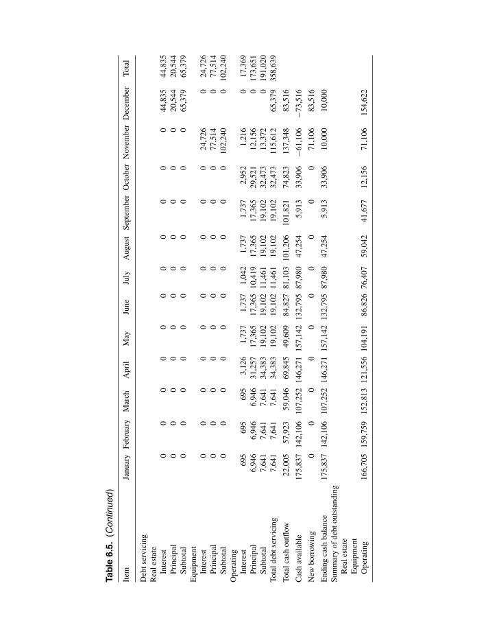
P1: SFK/UKS P2: SFK


Tab

le6.

5.(C

ontin

ued

)

Item

Janu

ary

Febr

uary

Mar

chA

pril

May

June

July

Aug

ust

Sept

embe

rO

ctob

erN

ovem

ber

Dec

embe

rTo

tal

Deb

tser

vici

ngR

eale

stat

eIn

tere

st0

00

00

00

00

00

44,8

3544

,835

Prin

cipa

l0

00

00

00

00

00

20,5

4420

,544

Subt

otal

00

00

00

00

00

065

,379

65,3

79E

quip

men

tIn

tere

st0

00

00

00

00

024

,726

024

,726

Prin

cipa

l0

00

00

00

00

077

,514

077

,514

Subt

otal

00

00

00

00

00

102,

240

010

2,24

0O

pera

ting

Inte

rest

695

695

695

3,12

61,

737

1,73

71,

042

1,73

71,

737

2,95

21,

216

017

,369

Prin

cipa

l6,

946

6,94

66,

946

31,2

5717

,365

17,3

6510

,419

17,3

6517

,365

29,5

2112

,156

017

3,65

1Su

btot

al7,

641

7,64

17,

641

34,3

8319

,102

19,1

0211

,461

19,1

0219

,102

32,4

7313

,372

019

1,02

0To

tald

ebts

ervi

cing

7,64

17,

641

7,64

134

,383

19,1

0219

,102

11,4

6119

,102

19,1

0232

,473

115,

612

65,3

7935

8,63

9

Tota

lcas

hou

tflow

22,0

0557

,923

59,0

4669

,845

49,6

0984

,827

81,1

0310

1,20

610

1,82

174

,823

137,

348

83,5

16

Cas

hav

aila

ble

175,

837

142,

106

107,

252

146,

271

157,

142

132,

795

87,9

8047

,254

5,91

333

,906

−61,

106

−73,

516

New

borr

owin

g0

00

00

00

00

071

,106

83,5

16

End

ing

cash

bala

nce

175,

837

142,

106

107,

252

146,

271

157,

142

132,

795

87,9

8047

,254

5,91

333

,906

10,0

0010

,000

Sum

mar

yof

debt

outs

tand

ing

Rea

lest

ate

Equ

ipm

ent

Ope

ratin

g16

6,70

515

9,75

915

2,81

312

1,55

610

4,19

186

,826

76,4

0759

,042

41,6

7712

,156

71,1

0615

4,62

2

P1: SFK/UKS P2: SFK



the outstanding balance on the operating capital loangoes down from $166,705 to $154,622. Thus, movingthe payments on the real estate and equipment loanseliminates five months of cash deficits and allows thefarm business to pay down a portion of its outstandingoperating capital debt.


Adams et al. (2001) used an annual cash flow budget asthe basis for an investment analysis to assess the eco-nomic feasibility of small-scale, commercial cultureof the southern bay scallop (Argopecten irradians con-centricus). A capital replacement schedule was used tocompare annual capital replacement costs of racks forcages and for longline systems to culture bay scallops.Growout cages were identified as the largest capital re-placement cash cost that occurs in Year 6. Sensitivityanalyses showed that the economic life of the growoutcages had a substantial effect on overall net returns.Extending the economic life through proper care andmaintenance increased returns while decreased eco-nomic life of growout cages due to poor maintenancesubstantially decreased net returns.

SUMMARY

This chapter discussed how to use cash flow budget-ing techniques to manage cash flow and avoid seriouscash flow problems. Cash flow problems can resultfrom a number of sources. These can include prob-lems associated with the timing of receipt of revenues,payment of farm expenses, and debt payments. Theprice, yield, and income risk in farming result in priceand cost fluctuations that can cause cash flow prob-lems. Prompt actions can often head off more seriouscash flow problems.

Pro forma cash flow budgets are used to project outmonthly cash flow for the upcoming year while thestatement of cash flows records the actual cash inflowsand expenditures. Comparing the projected and actualcash flow to date by month allows the farm manager tospot deviations early and devise actions to effectivelycorrect and avoid further cash flow problems.

Corrective actions for cash flow problems can takemany forms. Changing pond management strategiescan help when fish can be sold that can change thetiming of receipt of revenue. Effective planning canidentify ways to change the timing of payment of ex-penses. Debt payments can be rescheduled.

One of the key steps is to maintain proper recordsthat include projected and actual cash flow as well asdeviations from planned and anticipated cash flow.

REVIEW QUESTIONS

1. What is the difference between a cash flow budgetand a statement of cash flow?

2. Define and explain liquidity and its importance tothe farm business.

3. Describe the relationship between leverage, use ofcredit, and cash flow, using aquaculture examples.

4. Explain how rescheduling loan payments can beused to improve cash flow for an aquaculture farmbusiness.

5. Describe two aquaculture production manage-ment options that can result in improved cash flow.

6. Describe two measures of repayment.

7. Describe how to develop a cash flow deviationreport.

8. Describe the types of records needed to compareprojected and actual cash flows.

9. Compare profitability and liquidity.

10. Describe some of the problems involved in accu-rately forecasting prices and costs of aquacultureproducts and inputs.

REFERENCES

Adams, Charles M., Leslie Sturmer, Don Sweat, Nor-man Blake, and Robert Degner. 2001. The economicfeasibility of small-scale, commercial culture of thesouthern bay scallop (Argopecten irradians con-centricus). Aquaculture Economics & Management5 (1/2): 81–97.

Bjorndal, Trond. 1990. The Economics of SalmonAquaculture. Oxford: Blackwell Scientific Publica-tions.

Grisdale-Helland, Barbara, Stale J. Helland, and KurtKolstad. 2004. Salmon. In W.G. Pond and A.W. Bell(eds). Encyclopedia of Animal Science. Philadel-phia: Taylor & Francis, pp. 777–780.

P1: SFK/UKS P2: SFK


P1: SFK/UKS P2: SFK


7Managing Capital Assets in

Aquaculture Businesses

INTRODUCTION

Aquaculture operations tend to have large amountsof capital assets. The magnitude of the capital assetsin aquaculture businesses require that these assets bemanaged carefully. Key questions that need to be askedwith regard to the management of capital assets are:(1) how much total capital should be used; (2) how todecide when to replace capital assets; (3) whether topurchase or lease capital assets like ponds and equip-ment; and (4) how to monitor the use of capital assets.This chapter discusses issues related to decisions onthe capital requirements for various scales of aquacul-ture production. A format for making decisions relatedto replacing capital equipment and costs of capital ispresented. Trade-offs among purchasing, leasing, orcustom hiring are compared. The chapter concludeswith a discussion of monitoring the use of capital andrecord-keeping requirements.

HOW MUCH TOTAL CAPITALSHOULD BE USED?

Determining the amount of total capital to be used isprimarily a process of long-run planning. In the longrun, many different changes can be made. For example,the farm can be sold, it can double in size, or it can bedivided into half. It is because of this flexibility thateconomists say that all resources become variable inthe long run.

Economies of Scale

The question of the total amount of capital to be used ina business is also a question of how large the business

should be. This is because larger businesses requiregreater amounts of capital. A primary determinant ofthe economically optimal (best) size of a business isthe extent of economies or diseconomies of scale.

Economies of scale are represented by a decrease inthe per-unit cost of production as output (total produc-tion) increases (Figure 7.1). Economies of scale areused to identify the optimal or best size of farm, thefarm size that results in the lowest cost per pound ofproduction across the farm. The first step in an analysisof economies of scale is to develop an enterprise budgetfor each possible farm size. The farm size that resultsin the lowest cost per pound is the most economicalsize. If the costs of production per pound decrease asthe farm size increases, then economies of scale ex-ist. If, however, the cost of production increases as thefarm size increases, then diseconomies of scale exist.When economies of scale exist, the output increasesby a greater percentage than the increase in each ofthe inputs as farm size increases. Economies of scaleexist when there are increasing returns to scale suchthat production is more efficient (lower cost) due tolarger farm sizes.

Economies of scale are found in industries with highcapital costs. The high capital costs result in higherannual fixed costs; greater levels of production spreadthese fixed costs over the increased units of production.

Economies of scale in aquaculture businesses canresult from the adoption of larger pieces of equipmentor more advanced technologies. For example, a largerfeed wagon may allow the manager to feed more pondsbefore returning to the feed bin and may result in lowercosts per pound of fish produced than feeding with asmaller feed wagon. Similarly, a larger farm may beable to hire enough workers to seine their own pondsas needed rather than waiting to schedule a customAquaculture Economics and Financing: Management and


81

P1: SFK/UKS P2: SFK



Figure 7.1. Economies of scale in catfish foodfish production.

harvester who may not be available as often as wouldbe best.

Economies of scale can also result from division andspecialization of labor. Larger sizes of businesses canallow the labor to become specialized in certain tasksand thus become more efficient at that task. For exam-ple, a large farm with a dedicated seining crew can de-vote time to properly train that crew to seine efficientlywhereas a smaller farm with a generalized work forcemay not develop the same level of efficiency or mayhave to contract with a custom harvesting companythat may increase costs.

Other factors can contribute to economies of scale.These can include purchasing supplies in bulk at adiscounted price, or spreading a manager’s salaryover greater acreage and greater total pounds sold.For example, Figure 7.2 demonstrates that building

1 levee

4 levees

3 levees

2 levees

Figure 7.2. Levees for a single pond.

fish ponds in a “windowpane” fashion can reduce thecost/acre of pond construction. The major investmentcost in a pond-based aquaculture farm is building thelevees; the more levees, the higher the fixed costs ofconstructing the pond.

Constructing a 1-acre pond requires four levees, orfour levees per acre. However, if two 1-acre ponds areconstructed side by side, as in Figure 7.3, with a sharedlevee, the total number of levees required is seven, or3.5 levees per acre. Thus, the cost of levee constructionwill be less per acre by constructing ponds in a way thatminimizes the total number of levees to be constructed.

Diseconomies of scale can also occur when busi-nesses become too large to manage efficiently. Theevidence of diseconomies of scale is an increase inper-unit costs of production as the business gets larger

1 levee

5 levees

4 levees

2 levees 3 levees

6 levees

7 levees

Figure 7.3. Levees for two ponds with a shared levee.

P1: SFK/UKS P2: SFK


Managing Capital Assets in Aquaculture Businesses 83

and generates greater output. Coordinating and con-trolling the business becomes more difficult as the sizeof the overall business gets larger. The top managerbecomes more separated from the direct operations,and efficient coordination becomes more difficult withlarger scales of business.

Firm Growth

In businesses with economies of scale, larger firmshave a cost advantage in that the per-unit costs arelower for larger than for smaller farms. The realities oflower costs that result from economies of scale mustbe considered carefully in long-run planning for thegrowth of the farm.

The decision whether to increase the size of the busi-ness depends on what the optimal scale of productionis for that particular farm business and its market. Oncethe optimal size of the business has been determined,the extent of expansion that would be ideal will be thedifference between the optimal size of the business andthe current size of the business. This section describeshow to identify the optimal size of a business; how-ever, credit capacity and other factors may limit boththe amount and rate of growth that is possible for thebusiness.

Farms in industries with economies of scale haveincentives to grow to a larger size if the business hasresources available, its resources are allocated in asuboptimal manner, or it has savings from disposableincome. One major incentive for business growth isto operate more efficiently by achieving economies ofsize to enhance income-generating capacity.

The optimal scale or size of the business is deter-mined by developing a long-run average cost curve(LRAC). Figure 7.4 illustrates the development of anLRAC for a shrimp hatchery. The LRAC consists of a

0.001.00

2.003.004.00

5.006.00

7.008.00

1701501301109070503010

Million PLs per month

$/1,

000

PLs

Figure 7.4. Developing a long-run average cost curve for a marine shrimp hatchery.

series of short-run situations that can each be analyzedand combined into a comprehensive analysis of theeffects of a variety of long-run options. Each short-runaverage cost curve (SRAC) corresponds to a particularsize of the business. The LRAC line is drawn by con-necting the lowest points of each SRAC. The lowestpoint of the LRAC indicates which scale of businessis optimal.

In Figure 7.4, the two SRACs correspond to two dif-ferent sizes of shrimp hatcheries. In this example, thelarger hatchery results in lower costs of production andthe firm’s overall business plan should include plansto expand to achieve that size if the current business issmaller or plans to contract to that size if the currentbusiness is larger.

Increased financial leverage can result in increasedfirm growth, but the additional borrowing used to fi-nance new investment also increases financial risk.Risk comes from increased potential losses of equitycapital and increased variation in expected returns.High financial risk can affect the rate of growth inequity.

HOW TO DECIDE WHEN TOREPLACE CAPITAL ASSETS?

The decision to replace or trade a piece of equip-ment should involve consideration of a number of fac-tors. Should equipment be replaced only when fullyworn out or should it be replaced earlier? Consider-ations should include ownership and operating costs,reliability of the equipment, and the effects on cashflow and taxes. As equipment wears out, its repaircosts increase and can reach a level where it is moreeconomical to replace that piece of equipment. New,more efficient, equipment may be more economical aslong as acquiring the capital necessary to upgrade the

P1: SFK/UKS P2: SFK



technology does not result in adverse financial effectson the farm. If the farm has expanded in size, newequipment may be needed to operate the larger farmsize efficiently.

Capital budgeting techniques can be used to makedecisions as to when to replace equipment. Using cap-ital budgeting, the net present value (NPV) for eachnumber of years in the replacement period can be cal-culated. The period that yields the greatest NPV shouldbe selected. Another approach is to conduct a marginalanalysis that compares the gains from keeping the assetfor another time period with the gains from replacingit.

Equipment on aquaculture farms is a major por-tion that requires capital investment. In the enterprisebudgets described in Chapter 10, the total equipmentinvestment ranged from $138,100 to $1,471,121 andfrom $1,461/acre to $2,302/acre on the 60-acre to the1,007-acre catfish farms. Capital spent on equipmentcannot be used for other investments or expenses. Thevalue of what would be earned from using the capitalfor some other use is referred to by economists as anopportunity cost. The opportunity cost of investmentcapital used to purchase equipment is part of its totalcost.

The costs associated with owning equipment includethe initial purchase cost and interest rates if funds areborrowed to acquire the equipment while operatingcosts include fuel and lubricants, repairs, and mainte-nance of the equipment. Many of the fixed ownershipcosts consist of a one-time large outlay of cash forthe initial purchase that may be quite large. Anotherlarge part of the cost of owning equipment is its de-preciation, a noncash cost that is easily overlooked orignored in financial analysis and planning. Depreci-ation is a charge that reflects the loss in value of acapital good due to wear and tear, obsolescence, andage. Accounting for the costs of depreciation is a wayto spread the purchase price of a piece of equipmentacross its useful life to recover the original investmentamount.

The annual ownership costs of equipment can beabout 10–15% of its original purchase price. However,the annual ownership costs will vary with the type ofequipment, how it is maintained, its age, and currentinterest rates.

Calculating the ownership costs of a particularpiece of equipment can be complicated. The Amer-ican Society of Agricultural and Biological Engineers(ASABE) provides guidance to estimate these costs(www.asabe.org). The calculation involves the annual

capital recovery cost which is a measure of the annualownership costs of equipment.

ACRS = (purchase price − salvage value) × capital

recovery factor + (salvage value × interest rate)

The salvage value (the value of the equipment afterits useful life) is calculated by multiplying the orig-inal purchase price by the remaining value percent-age found on the ASABE’s web site. For example, a10-year-old tractor may have a remaining value of37%. If the tractor originally cost $60,000, its salvagevalue after 10 years of use would be $60,000 times0.37, or $22,200. The capital recovery factor (CRF)is an annuity factor that can be found in Table 14.6.Thus, the annual capital recovery factor (ACRF) forthe $60,000 tractor at an interest rate of 8% is:

ACRF = ($60,000 − $22,200) × 0.14903

+ ($22,200 × 0.08) = $7,409

It is important to note that the interest expense onthe value of the equipment is calculated to account forthe use of investment capital in that particular piece ofequipment.

Taxes (property and sales), insurance, and equip-ment storage costs are additional ownership costs ofequipment and pond assets. Some states do not chargepersonal property taxes on equipment, and sales taxesare variable across states. Insurance on equipment typ-ically costs about 0.8% of its average value with arange of 0.5–1.0%. Facilities to store equipment typ-ically cost about 2% (ranging from 0.5 to 3%) of theaverage value of the equipment.

The annual ownership costs for each piece of equip-ment can be compared by dividing the annual cost bythe estimated annual use (in hours used for each pieceof equipment). The result is a measure of the totalownership cost per hour of use. Fuel efficiency useof different pieces of equipment can be compared bydividing the gallons of fuel consumed by each pieceof equipment by the hours of consumption to obtaina measure of fuel cost per hour. These can be com-pared with the performance guidelines published bythe ASABE for different types of equipment and en-gine sizes.

The repair and maintenance costs of equipment canbe based on the accumulated repair costs over the lifeof the piece of equipment. The engineering cost iscalculated by multiplying the list price by the repairand maintenance cost percentage, which is calculated

P1: SFK/UKS P2: SFK



by dividing the accumulated repair and maintenancecost by the total hours of use over its useful life.

Operating costs of equipment include fuel and lubri-cation, repairs, and maintenance costs. Farm recordsprovide the best information on fuel and lubricationcosts. Tractor tests show that fuel consumption canbe estimated from the maximum power takeoff horse-power (hp) of a tractor. For gasoline tractors, the gal-lons of gasoline used per hour are 0.06 times the hp ofthe power takeoff unit, while for diesel units, it is 0.044times the hp of the power takeoff unit. Lubricants andfilters add an additional 10–15% of fuel costs.

Repair costs vary for various types of equipment andfor various levels of usage. However, agricultural en-gineers estimate that repair costs can range from 0.5 to9% of the original purchase price of the equipment foreach 100 hours of use. Repair costs typically increaseover time as equipment ages and increasing amountsof repairs are required.

Repairs and Maintenance versusDepreciation

One of the difficult decisions for a farm business ishow much capital to spend on repairs and mainte-nance. Over time, adequate maintenance and repair ofequipment can allow that equipment to be used for agreater number of years than if it is not maintainedand wears out more quickly. Some farmers attemptto survive by minimizing as many costs as possible,and repairs and maintenance can be some of the firstexpenses to be foregone in difficult economic times.

Monitoring the efficiency of equipment can providesome indication of when it may need to be replaced.One indicator of machinery efficiency is machineryinvestment cost per crop acre. This is calculated bydividing the current value of all crop machinery by thenumber of crop acres on the farm. Another measure,total machinery cost per crop acre, compares the oper-ating cost of the equipment. It is calculated by dividingthe total annual machinery costs, both ownership andoperating, by the number of crop acres.

The costs of repairs and maintenance will begin toincrease as equipment and ponds wear out. The wearand tear on equipment and ponds must be replacedand accounted for at some time or the farm will notbe able to continue to survive. Eventually, the depre-ciated value of the asset is very low and the costs tomaintain and repair the tractor or truck become exces-sive. A careful comparison of the annual costs of re-placing the capital item with the average annual costs

to maintain and repair that piece of equipment willprovide guidance on the best time to replace it. Thetiming of the replacement of equipment should takeinto consideration the pattern of cash flow and timethe purchase to coincide with a time period in whichthere is greater cash inflow. Debt payments should bescheduled for ease of payment. If fish prices are ex-pected to be low, deferring equipment replacement foran additional year may be preferable.

The Cost of Acquiring Capital

The costs a business pays for its financial capital are re-ferred to as the costs of capital. The liabilities listed onthe business’s balance sheet comprise the business’s fi-nancial capital. Debt and equity together constitute thedegree of a business’s financial leverage and the rela-tionship of debt and equity levels in the business reflectthe business’s capital structure. The cost of debt capitalshould be lower than the cost of the equity capital.

For family-owned farms, equity capital is providedby retained earnings (reinvesting farm profits) and un-realized capital gains from the farm. However, in con-trast to national financial markets that provide capitalfor large corporate businesses, retained earnings arehighly uncertain with a rate of growth not fast enoughfor large investments. Agricultural farm businesseshave thus relied heavily on borrowing and leasing.

Use of retained earnings also incurs an opportunitycost in that the funds are invested back into the businessinstead of spent by the family for some other activity.Costs of retained earnings can be thought of as therates of return needed to compensate for the familyconsumption that is foregone.

Acquiring capital results in interest charges typicallypaid to the lender from whom the loans are obtained.Various credit plans can be compared by calculatingthe cost of the various plans.

To compare the cost of different loans designed toacquire capital assets, the actual percentage rate (APR)of each can be calculated. The APR is calculated bymanipulating the following equation:

Periodic loan payment = net amount borrowed

× amortization factor.

This equation is solved for the amortization factor.The net amount borrowed is calculated by subtractingany non-interest charges and loan points or signingfees from the original loan amount. The periodic loanpayment is then divided by the net amount borrowedto identify the amortization factor. The value of the

P1: SFK/UKS P2: SFK



amortization factor calculated is then used to identifythe interest rate relative to the number of periods forthe loan by using Table 14.6. If there is more than onepayment a year, the interest rate is multiplied by thenumber of payments per year to obtain the annual rate.

The net present value (NPV) and the internal rateof return (IRR) can be used to compare the returns tothe possible alternatives to purchasing capital assets.The true cost of borrowing can be compared with theuse of these indicators. Chapter 13 presents details ofthe calculation and interpretation of NPV and IRR.

How Much Debt is Too Much?

New loans are frequently required to finance new cap-ital assets needed to expand the business by buildingor acquiring new ponds or purchasing new equipment.Each farmer or farm business has a certain level ofcredit capacity. It will be difficult for farmers to bor-row capital beyond their credit capacity because theincreased leverage would increase financial risk to anunacceptable level.

The business owner can use the financial statementsdescribed in this book to calculate important financialratios that shed light on this type of decision. Addi-tional debt results in two different types of concern:(1) short-term cash flow requirements and short-termdebt; and (2) solvency of the business and longer-termeffects of increased debt.

The short-term cash flow requirements and debt areevaluated with a cash flow budget (see Chapter 12for details on preparation and evaluation of cash flowbudgets). The debt-servicing ratio and the cash flowcoverage ratio, calculated from the cash flow budget,provide quick indicators of the effects on cash flow.The debt-servicing ratio divides the interest and prin-cipal payments by the cash inflow. Thus, smaller valuesare preferred and increasing values indicate increasingrisk of inadequate cash flow to meet financial pay-ments when due. The cash flow coverage ratio dividesthe cash inflow by the sum of the interest and principalpayments. Higher values are clearly preferred and de-creasing values over time indicate increasing financialrisk to the business.

In addition to these formal indicators, a quick lookat several lines on the cash flow budget can be use-ful. In particular, the line items that indicate the cashavailable, new borrowing, and outstanding operatingcapital debt on the cash flow budget provide insightinto the effects of additional borrowing. Decliningcash available, increased new borrowing, and increas-ing amounts of outstanding operating capital debt all

indicate that cash flow risk is increasing. These are acause for concern unless there is some realistic expec-tation of a major change in the next year.

The effects of additional debt to acquire new cap-ital assets on long-term debt, financial structure, andsolvency of the business must be evaluated from thebalance sheet (see Chapter 11 for details on prepara-tion of and interpretation of balance sheets). The networth on the balance sheet should generally increaseover time. Acquisition of new capital assets that re-quire new borrowing will increase both the liabilitiesand the assets on the balance sheet. The result of-ten is a short-term decrease in net worth. However,wise investments in new capital assets are those thatincrease profits over time. Increasing profits will re-sult in increased net worth. However, if a new capitalacquisition results in a large negative net worth, thefinancial risk may be unacceptable.

The debt/asset ratio provides a quick view of thesolvency of the business following additional capi-tal acquisitions. Lower debt/asset ratios are preferableand debt/asset ratios greater than one indicate that thebusiness is no longer solvent. Thus, if a new capitalacquisition increases the debt/asset ratio, but the valueremains below one, the additional debt level is not ex-cessive. A debt/asset ratio that exceeds one indicatespotential solvency problems. In such a case, a fullevaluation is needed to assess whether the increaseddebt/asset ratio is a temporary condition or whether itwould likely be lasting longer. Long-term exposure todebt/asset ratios above one is an unacceptable level offinancial risk that few businesses can sustain.

PURCHASING, LEASING, ORCUSTOM HIRING CAPITAL ASSETSSUCH AS PONDS AND EQUIPMENT

There are alternatives to purchasing equipment. If thefarm’s financial structure cannot withstand additionaldebt, machinery tasks can be either hired out to customoperators or the equipment can be leased.

There is no one rule of thumb for deciding whetherleasing equipment and ponds is better than purchaseof capital goods. The alternatives must be analyzedcarefully before making the decision. The decision asto whether to purchase or lease a piece of equipmentsuch as a tractor should be based on the estimated totaloverall costs associated with the possible alternatives.A tractor needed for the fish farm will provide the samebenefits in terms of production and revenue regardlessof whether it is purchased or leased. However, the costswill be different. Careful analysis should compare the

P1: SFK/UKS P2: SFK



cash outlay for purchase and leasing, adjusted for anytax savings that would be obtained from being ableto deduct expenses or depreciation. The lowest costoption would be the preferred option.

Leasing or renting equipment or ponds can be analternative to purchasing capital items. It provides anopportunity for a farmer to increase the size of thebusiness or to adopt more efficient technology with-out having the capital to acquire it outright. Leasingcan be a feasible way for young farmers to start out inthe business. One principal benefit of leasing or rent-ing is that lower initial payments may provide a bettercash flow pattern to cover other expenses in the year.Some lease rates may result in lower costs. Moreover,leasing may result in greater liquidity for the farm busi-ness, particularly in the earlier years. Leasing can alsoconserve working capital because the only liabilitiesincurred are those of the rental rates.

On the other hand, a high percentage of its capitalassets will have less collateral to use as a basis forincreasing its credit capacity. Ownership of ponds andequipment also increases equity for the farm business.Increasing equity enhances the balance sheet and con-tributes to owner’s wealth.

The costs of leasing are handled differently fromcosts associated with capital acquisitions in the anal-ysis of the farm’s finances. Rent and other expensesfrom leases are variable or operating costs rather thanfixed or ownership costs and are cash, not noncashexpenses. A lease will result in higher variable or op-erating costs. If fish prices are expected to decreasein the near term, revenue would decrease, and a leasemay not be the best choice. Moreover, high lease ratesmay not be profitable. Engle (2007) showed that catfishfarming was not profitable at certain pond lease ratesbut was profitable at other lower levels. The farmermust analyze his/her options carefully.

The annual amount of the rent and other lease ex-penses is entered into the enterprise budget and theincome statements as a variable cost. Leased assets,however, are not included on the balance sheet eitheras assets or liabilities. Thus, leasing does not affect thefinancial ratios of the business that are calculated fromthe balance sheet.

Leasing may increase a farmer’s credit over timeif working capital is conserved. However, if the cashflow demands of a lease are excessive, the lease may bedetrimental to the farm’s cash position. Such a situationcould negatively affect a farmer’s credit.

A farm that is highly leveraged (operating with ahigh debt load) and with low equity may not have thefinancial strength to assume additional debt. Leasing

ponds, tractors, or aerators may be the best option fora few years. During this time, some of the debt loadcan be paid down to a level that would allow for newloans to pay for purchasing new equipment.

Pond leases should include a legal description ofthe ponds and land to be leased, the length of timeover which the lease is valid, the amount of rent to bepaid, how and when payments are due, the names ofthe owner (known as the lessor) and the tenant (knownas the lessee), and the signatures of both. Pond leasesshould specify whose responsibility it is to maintainthe levees, mow the grass, and who pays for addinggravel to maintain the roads on top of the levees. Mostfarm leases are written for 1 year but contain a clausethat provides for automatic renewal from year to year.Pond lease rates in the southern portion of the UnitedStates can vary from about $100 to $350 per acre.

The lease agreement should stipulate when rent isto be paid. Lease payments should be entered into thecash flow budget to be certain that the lease paymentscan be made in a timely fashion. Cash flow problemscan occur if lease payments are required before thecrop will be marketed. If cash is not available, then thelease payments may need to be financed through short-term operating loans that increase total costs from theadditional interest charges. The timing of rent pay-ments should be negotiated along with the rental rate. Ifthe rent is due earlier in the production season, the riskis shifted to the grower from the owner and there shouldbe an accompanying decrease in the amount of the rent.Some leases require a prepayment and/or a security de-posit that must be accounted for in financial planning.

MONITORING CAPITAL USE

Part of managing capital efficiently involves continu-ous analysis of its use. The first general approach tosuch an analysis is to compare the performance of thefarm’s capital assets from one year to the next. Chap-ter 4 presents details of methods of doing this. Thistype of analysis shows the business’ progress fromone year to the next and how economic changes affectthe business. However, it can be difficult to sort outwhether the business’s performance is due to its man-agement or due to external economic effects. Anotherdisadvantage of this approach is that it relies entirelyon the past.

Another approach to monitoring capital use is tocompare the business’s performance to that of otherfarms. This method allows the farm to compare theirperformance indicators to those of other, similar farms.There are private firms and some university extension

P1: SFK/UKS P2: SFK



services that operate programs for a fee to do this.Farms then receive periodic statements that allow themto compare their farm’s performance on a number ofdifferent indicators with other farms that raise the samecrops.

RECORD-KEEPING SUGGESTIONS

Record-keeping is essential for managing capital as-sets. The fundamental records necessary to evaluatethe use of capital in the business are balance sheets(Chapter 11) and cash flow budgets (Chapter 12). Fromthese, the relevant ratios and indicators, described inChapter 4, should be calculated.

Managing capital assets also requires planning forthe use of capital on the farm. Hours used for eachpiece of equipment allow the manager to calculate thetotal ownership cost per hour of use and compare thisacross different types of equipment. Records of hoursof machinery use can be used to calculate machineryhours per acre or per pound of fish or shrimp produced.These records can form the basis for comparing thepotential value of newer or larger pieces of equipment.

Machinery cost records that include both ownershipand operating costs should be maintained. A depre-ciation schedule should be set up for each piece ofequipment and adjusted annually to show the loss invalue over the year as well as the current value. Withno repairs and maintenance, equipment and ponds willwear out more quickly and will then need to be re-placed in their entirety. It can be more expensive torenovate or repair ponds and equipment than it is topurchase them.

Tax and insurance costs, lease payments for anyequipment rental, and the cost of capital should berecorded, preferably by piece of equipment. Operatingcosts that should be monitored for equipment on thefarm include fuel and oil expenses, costs of spare partsin inventory, repairs, and any custom hires. Maintain-ing records of fuel use by piece of equipment providesa means to calculate and compare fuel efficiency acrossmachinery on the farm. Increasing values over time in-dicate when it would become profitable to replace thatpiece of equipment.

Complete records for a farm include repair andmaintenance costs for each type of capital asset inthe business. This list should match the depreciationschedule on capital assets that is used for income taxpurposes.

The profitability of capital is typically measuredby the return on capital. Chapter 13 presents a moredetailed discussion on its calculation. The return on

capital and the internal rate of return on capital usecan be calculated and maintained in the farm’s recordseach year.


The frequency of rebuilding or renovating ponds is aquestion relevant to pond-based farms and their strat-egy for managing capital assets. When pond leveesbecome too narrow for a feed wagon, hauling truck, orharvesting equipment to pass, production and outputof fish will suffer. Moreover, ponds silt in over timethrough erosion of the main levees. This results in theponds becoming too shallow. Shallow, silted-in pondsresult in weed problems and reduced capacity to storeoxygen. The result can be a reduction in fish yields andpossibly an increase in the feed conversion ratio.

An analysis of when it is appropriate to incur theinvestment required to renovate ponds would beginwith a tabulation of the costs and benefits that would beincurred through the renovation. Costs would includethe costs of contracting the equipment and labor forthe actual renovation, any lost production from havingthe ponds out of production for a time, and pumpingcosts required to fill the ponds again. Benefits wouldconsist of improved feeding rates, increased yields,and possibly lower feed conversion ratios.

Equipment used to renovate ponds can include abulldozer, bulldozer and box blade, bulldozer and dirtbuggy, or a trackhoe to pull up the levees. Renovat-ing a pond can cost on average $575/acre, but costscan range from $350 to $1,000/acre. Taking the pondout of production will result in lost production for thatperiod of time. For example, it may take 5 months todry out the pond, but this time can range from 3 to12 months. The actual renovation may take only2 weeks with a range of from 0.5 to 3 weeks.

To estimate the costs associated with the time thatthe pond is out of production requires several assump-tions. In the best case scenario, the pond could startdrying out in February and could be dried by April.Thus, 1 month of production would be lost for dry-ing, an additional 2 weeks for renovation, and another2 weeks for pumping up the pond again. In the worstcase, the entire growing season could be lost. Thiswould entail a 6-month period that extends from mid-April through mid-October. Net daily yield in pondscan be 19 lb/acre/day for a 7,000 fish/acre stockingdensity, but can be as much as 24 lb/acre/day acrossall densities. In the worst case scenario, net daily yieldfrom single-batch production with 0.6 lb stockers was31–40 lb/acre/day.

P1: SFK/UKS P2: SFK



Table 7.1. Renovation Costs for a Variety of Scenarios.

Large fish scenarios

Category Best case scenario costs Worst case scenario costs (31 lb/acre/day) (40 lb/acre/day)

Renovation $7,475 $7,475 $7,475 $7,475Lost production $815 $3,011 $3,906 $5,040Pumping cost $1,040 $1,040 $1,040 $1,040Total $9,330 $11,526 $12,421 $13,555lb catfish to cover costs 13,328 16,466 17,744 19,364lb/acre 1,025 1,267 1,365 1,490

Putting these together for a 13-acre pond with2 months of lost production (best case scenario) wouldhave renovation costs of $7,475, lost production of$815, and pumping costs of $1,040, for total costsof $9,330 (Table 7.1). It would take an additionalweight of 13,328 lb of catfish to cover these costs,or 1,025 lb/acre (calculated at a price of $0.70/lb). Inthe worst case scenario, the pond is out of productionfor a longer time and the lost production costs increaseto $3,011 for a larger total cost of $11,526. Thus, forthe worst case scenario, 16,466 lb of catfish are re-quired to cover costs, or 1,267 lb/acre. With yields of31 lb/acre/day, the cost of the production lost increasesfurther to $3,906 and would require a total of 17,744 lbof catfish, or 1,365 lb/acre. If net daily yield was40 lb/acre/day, the lost production cost would increaseto $5,040 and would require 19,364 lb of catfish tocover costs, or 1,490 lb/acre/day.

In summary, the longer the pond is out of production,the greater the renovation cost. The more productivethe pond, the greater the overall renovation cost.

In terms of the benefits, there was no significantdifference in the feed conversion ratio between 1 and

6 years following renovation (Figure 7.5). Figure 7.5shows the additional feed cost if the feed conversionratio increases, but the yield stays the same.

The decision as to when to renovate ponds requiresan investment analysis because renovation is a long-term capital decision. For the investment analysis, re-turns and costs, including renovation costs, must beestimated for each year for 10–20 years. The NPV iscalculated to measure the profitability of the proposedinvestment.

Figure 7.6 shows the net returns by year if the pondis not renovated, with hypothetical feed conversionratios. Figure 7.7 shows the net returns for 7 yearsfollowing renovation. In contrast, Figure 7.8 showsthe pattern of net returns if ponds are renovated every10 years.

How do we determine which scenario is the mostprofitable? Table 7.2 compares the NPV without reno-vation, renovating every 7 years, 10 years, or 13 years.Figures 7.7 and 7.8 demonstrate negative net returnsin those years that ponds are renovated, due to thecost of the renovation. The highest NPV (most prof-itable) occurs when ponds are renovated once every

0

2,000

4,000

6,000

8,000

10,000

0.60.50.40.30.20.1Increase in FCR

Add

ition

al fe

ed c

ost f

orsa

me

leve

l of y

ield

$/13-acre

Cumulative

Figure 7.5. Additional feed cost if feed conversion ratio increases but yield remains the same as pond ages.

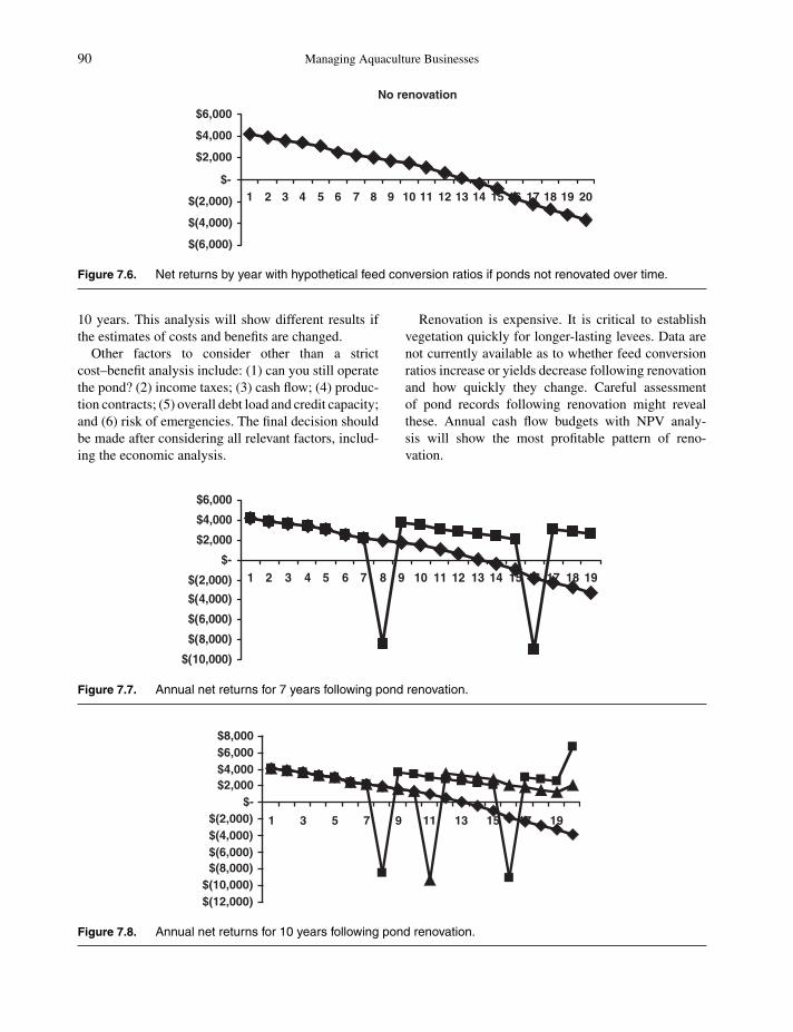
P1: SFK/UKS P2: SFK



No renovation

$(6,000)

$(4,000)

$(2,000)

$-

$2,000

$4,000

$6,000

2019181716151413121110987654321

Figure 7.6. Net returns by year with hypothetical feed conversion ratios if ponds not renovated over time.

10 years. This analysis will show different results ifthe estimates of costs and benefits are changed.

Other factors to consider other than a strictcost–benefit analysis include: (1) can you still operatethe pond? (2) income taxes; (3) cash flow; (4) produc-tion contracts; (5) overall debt load and credit capacity;and (6) risk of emergencies. The final decision shouldbe made after considering all relevant factors, includ-ing the economic analysis.

Renovation is expensive. It is critical to establishvegetation quickly for longer-lasting levees. Data arenot currently available as to whether feed conversionratios increase or yields decrease following renovationand how quickly they change. Careful assessmentof pond records following renovation might revealthese. Annual cash flow budgets with NPV analy-sis will show the most profitable pattern of reno-vation.

$(10,000)

$(8,000)

$(6,000)

$(4,000)

$(2,000)

$-

$2,000

$4,000

$6,000

19181716151413121110987654321

Figure 7.7. Annual net returns for 7 years following pond renovation.

$(12,000)$(10,000)

$(8,000)$(6,000)$(4,000)$(2,000)

$-$2,000$4,000$6,000$8,000

1 3 5 7 9 11 13 15 17 19

Figure 7.8. Annual net returns for 10 years following pond renovation.

P1: SFK/UKS P2: SFK



Table 7.2. Net Present Value with DifferentFrequencies of Pond Renovation.

Option Net present value

No renovation $16,754After 7 years $20,150After 10 years $20,931After 13 years $20,531


Cyrus and Pelot (1998) developed a database planningsoftware system for management of scallop farms.Simulations demonstrated the required allocation ofcapital resources among various types of nets. It tracedthe use of optimal capital through different stages inthe production process until the operation reached asteady state.

SUMMARY

This chapter reviewed decisions related to managingthe capital assets in the farm business. These assets arethose that are used by the farm business for more thana year. The fundamental concept of economies of scaleis reviewed because many aquaculture businesses ex-hibit strong economies of scale due to the relativelyhigh proportion of capital costs in aquaculture busi-nesses. Economies of scale exist due to spreading pondconstruction costs across greater levels of output, shar-ing equipment and management across greater levelsof output, and the opportunity to purchase inputs suchas feed at a lower cost. The long-run average cost curve(LRAC) is used to identify the optimal size of a busi-ness by finding the size of business associated with theshort-run average cost curve that has the lowest cost.

Managing capital assets efficiently includes makingdecisions to be able to use the proper size of equip-ment, maintain it in good operating condition, and tomake appropriate decisions related to its timely re-placement. The decision when to replace equipment iscomplicated and the timing of replacement can affectthe financial structure of the business as well as itscash flow position.

Capital acquisition can occur through custom hirearrangements or through leasing ponds and other fa-cilities as well as equipment. The decision to purchaseor lease should be made after careful analysis of theeffect on the business’s financial position and its cash

flow. Assessment of how much debt is too much isneeded to avoid incurring debt loads that entail exces-sive financial risk.

REVIEW QUESTIONS

1. What are economies of scale? Give several ex-amples of aquaculture industries that exhibiteconomies of scale.

2. What creates economies and diseconomies ofscale? Give aquaculture examples of each.

3. How do economists identify the optimal size of abusiness? Draw the appropriate curve and describehow it is derived.

4. What are the trade-offs between purchasing andleasing ponds and equipment? How are equipmentcosts treated differently in financial analyses ifequipment are purchased as compared to leasing?

5. How does a farm owner assess whether incurringadditional debt will incur excessive financial risk?

6. Describe two indicators of machinery efficiencyand explain how each is calculated.

7. Compare the types of costs associated with own-ership of equipment and those associated with op-erating the equipment.

8. What types of records should be maintained oncapital assets of the business, both long-term fa-cilities and equipment?

9. What are the costs associated with borrowing cap-ital?

10. Which financial indicators provide the best indica-tion of whether additional debt is feasible or not?

REFERENCES

American Society of Agricultural Engineers.www.asabe.org. Accessed March, 2009.

Cyrus, Pemberton and Ronald Pelot. 1998. A site man-agement system for shellfish aquaculture. Aquacul-ture Economics and Management 2(3):101–118.

Engle, Carole R. 2007. Arkansas Catfish ProductionBudgets. Arkansas Cooperative Extension ProgramMP466. Pine Bluff, AR: University of Arkansas.

P1: SFK/UKS P2: SFK


P1: SFK/UKS P2: SFK


8Managing Risk in Aquaculture

Businesses

INTRODUCTION

The level of risk in an aquaculture business requiresthat managers plan to make adjustments when negativeoutcomes occur so that the business will be successful.The goal of managing the risk in a business is to im-prove the probability of success. However, even withthe very best management, profits are not guaranteed.Well-thought-out and carefully planned decisions canstill result in poor outcomes. Moreover, higher prof-its are frequently associated with greater risk of losses.The key is to evaluate decisions based on the objectivesof the business, not in reaction to previous decisions.Good decisions and strategies over time will result inpositive outcomes in spite of the occasional negativeoutcomes.

This chapter focuses specifically on strategies tomanage risk. Chapter 16 presents details of what con-stitutes risk, various sources of risk, and how to mea-sure risk. For those unfamiliar with how economistsdefine and measure risk, reading Chapter 16 prior tothis chapter would be worthwhile.

PRIORITIZING RISK

A manager of an aquaculture business must accountfor risk in each phase of the business. Planning be-gins with careful identification of the types of risk thatthe business is likely to face in the upcoming plan-ning term. The second step is to identify the possibleoutcomes from each type of risk.

The process of prioritizing risk requires assessmentof the potential impact on the business as a result of thevarious sources of risk and an estimate of the probabil-

ity of that type of effect occurring. Careful evaluationof the combined effects of both these criteria allows themanager to identify those likeliest to cause the greatestproblems.

Consider Figure 8.1 related to assessment of therisk associated with the discovery of viral hemorrhagicsepticemia (VHS) in one’s state. This disease broke outin the United States in the Great Lakes area and hasresulted in development of regulations that prohibitthe transport of live fish from VHS-positive states. Afish farm whose market requires interstate shipment oflive fish in the United States should carefully weighmanagement options related to the risk of their statebecoming VHS-positive. According to Figure 8.1, afarm located in a state adjacent to a VHS-positive statewould have a higher probability of VHS spreading. Thepotential impact would be very high because the resultlikely would be a loss of all sales to other states becauseregulations would prohibit interstate shipment. Thus,steps to develop biosecurity protocols or to engage inan inspection and certification program would likely berecommended to minimize these risks. However, foodfish growers who sell to a processing plant in the samestate may still have a high probability of experiencingsome effect, but the potential negative impact on thebusiness would be lower. Thus, the need for actionwould be less.

METHODS TO ORGANIZE RISKSAND STRATEGIES

A decision tree is a useful way to organize the varioustypes of risks and the alternative strategies for man-aging them. Figure 8.2 illustrates a decision tree foran example of alternative strategies for coping withrisk on a shrimp farm. The decision tree consists of


93

P1: SFK/UKS P2: SFK



Very highVery low

Unlikely

Certain

concern

Little Bearswatching

Highest

concern

Bearswatching

Potential impact

Pro

bab

ility

of

occ

urr

ence

of

a ri

sk f

acto

r

Figure 8.1. Prioritizing risk.

branches and nodes that denote decisions and is drawnfrom left to right. In Figure 8.2, there are three possibleoutcomes (good, average, poor) for each alternativeoption.

The options considered in Figure 8.2 consist of threestocking options for the shrimp ponds: (1) 1 postlar-vae/m2; (2) 1.5 postlarvae/m2; or (3) 2 postlarvae/m2.

The probability of disease incidence varies from yearto year and with stocking density. The price receivedfor shrimp is based on the size of the shrimp producedand the size of shrimp produced varies with the stock-ing density. Figure 8.2 shows the probabilities of good,average, or poor outcomes from each stocking densityand the net returns associated with each outcome for

Good

Good

Good

Poor

Poor

Average

Average

Average

Poor

0.1

0.5

0.4

0.2

0.5

0.3

0.3

0.5

0.2

X

X

X

X

X

X

X

X

X

$1,000

$800

–$100

$900

$700

–$50

$800

$500

$100

Net returns($/ha)Probability

Diseaseoutcomes

Stockingstrategy

Expectedvalue ($)

$100

$400

–$40

$180

$350

–$15

$240

$250

$20

1/m 2

2/m2

1.5/m2

Figure 8.2. Decision tree for shrimp stocked at different densities.

P1: SFK/UKS P2: SFK


Managing Risk in Aquaculture Businesses 95

Table 8.1. Payoff Matrix for Shrimp Stocking Rate.

Stocking density

Regrets 1/m2 1.5/m2 2/m2

DiseaseOutcomes 1/m2 1.5/m2 2/m2 P $ P $ P $

Good $200 $100 $0 0.3 800 0.2 900 0.1 1,000Average $300 $100 $0 0.5 500 0.5 700 0.5 800Poor $0 $150 $200 0.2 100 0.3 −50 0.4 −100Expected value n.a. n.a. n.a. n.a. 460 n.a. 515 n.a. 510Minimum return $0 $100 $0 n.a. 100 n.a. −50 n.a. −100Maximum return n.a. n.a. n.a. n.a. 800 n.a. 900 n.a. 1,000Range n.a. n.a. n.a. n.a. 700 n.a. 950 n.a. 1,100Maximum regret $300 $150 $200 n.a. n.a. n.a. n.a. n.a. n.a.Expected regret $210 $115 $80 n.a. n.a. n.a. n.a. n.a. n.a.

each strategy. The expected net returns are determinedby multiplying the probability of occurrence of eachby its expected net returns and adding up the results.Thus, the expected net returns for a stocking rate of 1postlarvae/m2 are $510/ha (sum of $240/ha, $250/ha,and $20/ha), $515/ha for 1.5 postlarvae/m2 (sum of$180/ha, $350/ha, and −$15/ha, and $460/ha (sumof $100/ha, $400/ha, and −$40/ha) for the 2 postlar-vae/m2 stocking density.

Another way to organize information on the relativevalues of alternative strategies is to develop a payoffmatrix. A payoff matrix is developed in the form of atable instead of a decision tree (Table 8.1). The payoffmatrix indicates the returns possible from a particu-lar action. The resulting values are identical to thosein Figure 8.2. Typically, a payoff matrix includes justone decision and one set of events. However, Table8.1 shows a payoff matrix for the three shrimp stock-ing densities from Figure 8.2. The possible events arelisted on the left side and the choices are indicatedacross the top. The returns expected from each choiceare calculated for each combination.

A regret matrix indicates the potential returns lostby not choosing the best option. For example, Table8.1 also shows the regrets the manager would have bynot choosing the other shrimp stocking densities. Forexample, if outcomes in that year are good, and themanager chose to stock at a low density, he/she wouldhave earned $200/ha less than if he/she had chosenthe highest density. However, if outcomes would bepoor that year, the manager would have no regrets (0)if he/she had stocked at the low rate. If he/she hadstocked at the high rate, the regrets would be $200/ha

because of the differences in net returns between the1/m2 and 2/m2 stocking densities when outcomes arepoor. The regret matrix also includes a summary ofthe maximum regrets for each stocking density and theexpected regrets. The expected regrets are calculatedby multiplying the regret value for each outcome by itsprobability and then summing them. Decision makersseek decisions with higher payoffs and lower regrets.A regret matrix can be combined with a payoff matrixin the same table with net returns demonstrated forboth payoffs and regrets, as in Table 8.1.

Decision Criteria for DecisionMaking

Economists have developed several types of decisionrules as a framework for making decisions related torisk. It is important to recognize that there are differ-ences in the results obtained from use of the differenttypes of decision rules. Factors that must be consid-ered in order to select the appropriate decision ruleinclude: (1) the decision maker’s attitude to risk; (2)the financial condition of the business; and (3) the cashflow requirements, among others.

The various decision rules include: (1) maximin(maximization of the minimum possible returns);(2) minimax (minimization of maximum possible re-grets); (3) most likely outcome; (4) maximum ex-pected value; (5) risk and returns comparison; (6)safety first; and (7) break-even probability. With themaximin rule for returns or payoffs, the option cho-sen is the one with the largest minimum returns.Thus, this decision rule focuses on downside risks and

P1: SFK/UKS P2: SFK



selects those options that will generate higher returnsduring the worst-case outcomes. The minimax crite-rion also focuses on downside risk but is based onregrets rather than payoffs. It is used to select the op-tion with the smallest value of maximum regrets. Themost likely outcome is based on the outcome with thehighest probability of occurrence and then selects thestrategy with the highest net returns for that partic-ular strategy. This is one of the easiest strategies toapply.

The maximum expected value decision rule will se-lect the alternative that has the greatest expected value(weighted average of the net returns multiplied timesits expected net returns). This decision rule does notaccount for the variability that may occur with the dif-ferent outcomes. Thus, the maximum expected valuedecision rule would be used primarily by risk-lovingmanagers.

The risk and returns comparison takes into consid-eration both the level of risk and the level of returnsexpected from each alternative strategy. It results inrejecting strategies with lower expected returns andhigher risks than other strategies. This decision rule ispreferred by managers who are more risk averse.

The safety-first decision rule results in selection ofthe best possible results of the worst-case scenario.In this rule, the emphasis is on managing the mostnegative outcomes because outcomes that are morepositive than expected do not result in financial prob-lems for the business. Financial problems arise fromthe negative, not the most positive outcomes. This ruleis particularly useful for businesses in difficult finan-cial positions, those that may not survive another badyear.

The break even probability decision rule weighs therisk of losses against the expected average return. Cu-mulative density functions are calculated for each al-ternative that allows for comparison of the variousalternatives.

TECHNIQUES TO HANDLE RISK

Techniques to reduce risk attempt to reduce the vari-ability of outcomes. This can be achieved by: (1) set-ting a minimum income or price level; (2) maintainingas much flexibility for decision making as possible; or(3) improving the ability of the business to bear risk.There are a variety of alternative strategies that havepotential to mitigate each type of risk. Each businessshould identify those that are feasible and practical forits situation.

The risk associated with each needs to be estimatedand the expected returns and trade-offs evaluated foreach alternative. The alternative strategies for cop-ing with the risks identified are known as decisionstrategies.

Tools for Managing Production Risk

Skilled Management

The riskiness of aquaculture requires skilled manage-ment. Skilled managers can reduce risk by maintainingfacilities and equipment in good repair. For example,aerators that function properly will minimize the riskof losses due to oxygen depletion. Skilled managerswho subscribe to trade journals, market news services,and those who attend educational meetings will be ina better position to minimize risk by making better-informed decisions than managers who do not stayabreast of current conditions and the latest research.Contracting experts to monitor specific aspects of thebusiness can help to be prepared to manage adverseconditions. Lawyers, accountants, and fish health ex-perts may be valuable resources.

Flexibility

Flexibility, in and of itself, does not affect risk, buta firm that is more flexible has the ability to makechanges that can help it to find ways to adjust andcope with risk. Aquaculture businesses tend to haverelatively high fixed costs. The high fixed costs reflectthe level of long-term assets that are more difficultto adapt and change as conditions change. Short-termassets can be sold more quickly and frequently in re-sponse to adverse conditions. However, there can be atrade-off between economies of scale (lower per-unitcosts of production) that are typically achieved withgreater capital investment and higher fixed costs. Thegreater efficiencies obtained from larger-sized opera-tions are often achieved at the expense of flexibility.On the other hand, greater flexibility may reduce riskbut will likely result in a less-efficient business.

Farm investments that can be used for multiple pur-poses can increase flexibility of the farm. Buildingsand equipment that can be used for multiple enter-prises will provide greater flexibility than buildingsand equipment that are highly specialized.

Crops with shorter production cycles reduce risk byproviding greater flexibility and opportunities to recap-ture costs sooner. This is because revenues are createdmore quickly and more frequently. Greater cash inflow

P1: SFK/UKS P2: SFK



to the business provides greater liquidity and providescash reserves to adjust to changing conditions. Raisingfingerlings, for example, can result in a faster cashturnaround time than raising food fish.

Share Leases

Crop and livestock share leases apportion risks be-tween the tenant and the landowner. This is becauseboth expenses and revenue from the sale of crops aretypically split between the tenant and the landowner.Share leases are not as common in aquaculture as inother forms of agriculture, but can offer a way to spreadproduction cost risks.

Long-term Contracts with Suppliersand Buyers

Long-term contracts for input supplies will reduce riskby stabilizing prices of inputs or products. For ex-ample, farmers who book feed in advance enter intoa long-term contract. The farmer then is protectedagainst rising prices of feed for the quantity of feedbooked.

Diversification

Identifying stable enterprises is another technique thatcan be used to reduce production risk. Some types ofcrops are more stable in terms of generating incomethan others are. Diversifying production on the farmcan reduce risk by producing more than one crop if theprice of that crop varies in an opposite direction fromthe other. If the second crop produces high revenues inyears when revenues from the first crop are likely tobe lower, producing both will minimize overall pricerisk across the business. The key is for the prices andyields of the different crops produced to have highsand lows at different times.

Diversification can reduce the total variability in netreturns by pooling several types of income-generatingactivities. Investments that entail greater risk usuallyalso have greater potential for higher net returns. Thus,strategies designed to reduce risk are usually accom-panied by lower returns.

Correlations can be calculated to measure howprices and yields are related. If prices and yields ofthe two crops are positively correlated, it means thatthey will both be high at the same time or that theywill both be low at the same time. With positivelycorrelated prices and yields, diversification will havelittle effect on reducing risk. Risk reductions will oc-

cur when the prices and/or yields of the two crops arenegatively correlated. Crops with strong yield correla-tions frequently will also have positive correlations forprice because the quantity sold of a commodity willaffect its price.

However, diversification across the farm may in-crease costs by complicating management. A farm thatspecializes in only one type of product may have higherreturns resulting from improved efficiencies obtainedthrough specialization.

Larger aquaculture companies may be able to di-versify across geographic areas. Geographic diversifi-cation can result in greater reductions in risk becauseproduction is spread over a wide area with differentseasons and different price variations.

Diversification strategies may also involve nonfarmsources of revenue to counteract the effects of priceand production risk. These activities can include in-vesting in stocks and bonds, working off the farm togenerate off-farm revenue, or hedging in futures con-tracts. Renting versus owning capital assets requiredfor aquaculture production may have different effectson risk, particularly if the farm business has consider-able financial risk due to being highly leveraged.

Tools for Market Risk

Market risk results primarily from fluctuations in mar-ket prices. Techniques that can be used to managemarket risk include: (1) inventory management; (2)contract sales and hedging; (3) forward contracting;and (4) marketing cooperatives.

Inventory Management

Holding fish to wait for higher prices can be a strategyto manage market risk because prices of many com-modities are seasonal. This can be particularly advan-tageous for farmers raising new aquaculture speciesthat are competing with wild-caught product. If thesupply of the wild species is seasonal, prices likelywill be seasonal. If the aquaculture grower can man-age to sell inventories during the times of high prices,there could be an advantage, at least until aquacul-ture production increases to high levels. For example,Chen et al. (2008) demonstrated that monthly pricesof summer flounder range from a low of $0.88/lb inJanuary to $1.26/lb in April. Some entrepreneurs havetaken advantage of this price seasonality by transfer-ring flounder caught in the wild to tanks on shorein Virginia, on the east coast of the United States(Kauffman 2004). The flounder were held and fed for

P1: SFK/UKS P2: SFK



several months and then sold in the live fish market inthe northeast of the United States. Gross margins of$4/lb were obtained as compared to $0.25/lb or lowerin the iced fish market.

Managing inventory can provide opportunities tospread sales over time. Such a strategy sometimes canspread the risk of varying market prices by selling bothduring times of low and high prices. Continuous pro-duction systems, as practiced in aquaculture segmentssuch as channel catfish in the United States, have thepotential to sell throughout the year. Spreading salesis more effective with crops that are not seasonal.

This strategy provides no protection from downsiderisk because prices could fall as inventories are held.Moreover, holding inventories of live product incursadditional risk of losses due to disease. Diseases couldreduce the quantity of marketable yields. Holding cropinventories also subjects the farmer to the risk thatprices will fall further in the future.

Forward Contracting

Contract sales can stabilize prices, especially if con-tracts signed are long-term. Contracts may also specifymanagement practices to be associated with the pro-duction of that commodity.

Forward price contracts exist for many grain andlivestock buyers. Forward contracting protects againstdeclines in prices. The disadvantage is that forwardcontracting also prevents the individual from gainingduring times of rising prices.

Contracting with a buyer to sell product at a certainprice in the future has the benefit of stabilizing marketprices for the farm; more stable prices reduce mar-ket risk. Moreover, a forward sales contract may beviewed favorably by lenders who are concerned withdownward price risk.

However, forward contracts restrict the farm to spe-cific production performance standards, harvest condi-tions, and terms of sale. If the contract calls for deliveryof a specified amount and yields fall short, the farmermay need to purchase additional product to meet theterms of the contract.

Futures Contracts and Hedging

Futures contracts are common for grain commodities.For example, the Minneapolis Grain Exchange hastraded wheat for over 110 years. Futures markets tendto enhance cash markets, but no one is required tophysically deliver or receive the product.

The prices of futures contracts tend to move in thesame manner as cash prices. The difference betweenthe futures contract price and the cash market price isreferred to as the basis.

A futures contract is an agreement to either deliveror receive a certain quantity and grade of a specificcommodity during a designated delivery period (thecontract month). The contract includes information onwhere the commodity would be delivered and any ad-justments in price from substituting a different speciesor size.

Selling a commodity futures contract instead of thecommodity itself allows a buyer or seller to set a mar-ket price for that quantity of product. The process ofbuying and selling futures contracts is known as hedg-ing. Hedgers enter the market to protect themselvesfrom market risks. Hedgers participate to reduce mar-ket risk associated with either rising or falling shrimpprices.

To protect against price declines, a farmer would buythe right to sell a futures contract (known as a “put”option) at an established price. A shrimp grower canbuy a “put” option to insure against decreases in cashprices. The “strike” price is the level of price protectionselected. A put option with a strike price of $4.50 anda premium of $0.20 enables the farmer to protect anet sales price of $4.30/lb (strike price—premium).For example, a shrimp producer who intends to sellshrimp during the next month could enter the futuresmarket to sell futures contracts. This is known as a“short” position. A shrimp grower, in a short position,is locking in a price for future sales.

Call options (the right to buy a futures contract at anestablished price) can be used to establish a maximumpurchase price for a commodity. Buying a call optionprovides insurance against price increases. A call op-tion with a strike price of $4.50 and a premium of$0.20 enables the individual to protect a net purchaseprice of $4.70/lb. These can be useful for inputs, suchas soybean meal for fish feeds.

For example, a buyer for a major restaurant chainwho will need to buy shrimp to serve in the restaurantsa month from now could enter the futures market to buyfutures contracts. This is known as a “long” position.A shrimp buyer in a long position (the buyer of futurescontracts) is locking in a price for future purchases ofshrimp. A buyer has the right, but not the obligation, tobuy or sell futures contracts at a predetermined priceat any time until the option’s expiration date.

Speculators provide the capital, risk capital, and liq-uidity needed for those who wish to use the futures

P1: SFK/UKS P2: SFK



market as a way to hedge prices. Speculators are bet-ting that the market will rise or fall.

Hedging for aquaculture growers is difficult be-cause there are no futures markets for the majorityof aquaculture products. Brokers require margins thatdecrease the benefits to farmers. Moreover, sometimesthe product specifications may not match well with thecapabilities of the farm and preclude participation infutures markets.

There have been some experiments with futuresmarkets for aquaculture commodities such as shrimp,with varying amounts of success. The MinneapolisGrain Exchange began to trade futures contracts forfarm-raised and wild white shrimp in 1993 and thenadded a contract for farm-raised giant tiger shrimp in1994.

There were two main contracts for shrimp: (1) 5,000lb of raw, frozen, headless, shell-on 41–50 count whiteshrimp (Penaeus vannamei, P. occidentalis, P. schmitti,P. merguiensis, and P. setiferus); (2) 5,000 lb of raw,frozen, shell-on 21/25 count farm-raised giant tigershrimp (P. monodon). The contracts were standard-ized so that they could be exchanged. However, theshrimp futures market was ultimately closed. A majorproblem of the shrimp futures market was the lack ofhomogeneity of the product (Martinez-Gamendia andAnderson 2001). Shrimp come in many different sizesand the fixed premium/discounts used to account forthe price differentials turned out to be inadequate.

Marketing Cooperatives

Marketing cooperatives have had some success in sta-bilizing farmers’ returns. Forming a cooperative pro-vides an opportunity to pool product from across dif-ferent farms. Cooperative members can develop mar-kets jointly. By doing so, storage, sales, and pric-ing functions can be transferred to a larger company.The larger company can supply larger buyers, de-velop longer-term contracts, and take advantage ofeconomies of scale with regard to marketing func-tions. Marketing cooperatives require knowledgeablemanagement. With skilled management, the market-ing cooperative can increase profit through its size andspecialization.

Tools for Managing Financial Risk

Management plans that result in adequate liquidity andsolvency can help to reduce financial risk. Maintainingadequate levels of liquid reserves will reduce financialrisk. Cash accounts that are maintained to provide cashduring emergency situations are a way of providinginsurance for the farm from the farm’s own resources.

Using fixed interest rates stabilizes the amount ofinterest payments. Fixed interest rates may be higherthan variable rates, but they protect against rising in-terest rates. Knowing what the interest payments willbe over time allows the manager to plan for timelypayments.

With careful planning, capital expenditures can bepostponed if financial conditions are not favorableand then made when cash is available. Flexibility inscheduling the purchase of assets will help to reducerisk in the business.

Use of self-liquidating loans (those repaid from saleof the loan collateral) will reduce financial risk. Es-tablishing operating loans based on the inventory offish raised would be an example of a self-liquidatingloan. However, many banks are hesitant to allow use ofswimming inventory as loan collateral, primarily dueto difficulties in accurately estimating the quantity offish inventory on the farm.

Credit Reserves

Maintaining a credit reserve will reduce risk becauseit provides for a ready source of additional borrowingcapacity. Maintaining a sound relationship with one’sbanker will help to maintain a reserve of credit (ad-ditional borrowing capacity that can be drawn uponduring adverse financial times). A sound relationshipwith the lender may help to obtain approvals to carryover loans, defer payments during adverse conditions,or to refinance high debt loads. Thus, working withone’s lender is an important risk management strategyfor many farmers.

Sensitivity analyses of liquidity and financial riskcan be done to assess the effects of variations in farmrevenue, farm expenses, and interest rates on the finan-cial risk in the business. The percent that farm revenuecan decline and still meet cash flow requirements iscalculated by dividing the excess cash available by thetotal cash available. These values are obtained fromthe cash flow budget. Greater detail on the mechanicsof cash flow budgets can be found in Chapter 12. Thepercent that farm expenses can increase and still meetcash flows is calculated by dividing the excess cashavailable by the cash operating expenses. The percentthat interest rates can increase and still meet cash flowsis measured by dividing the excess cash available bythe total liabilities.

Long-Term Debt to Equity

Increasing equity in the business also reduces riskbecause it provides the solvency and much of the

P1: SFK/UKS P2: SFK



liquidity of the business. Dividing the long-term debtby the equity (and multiplying by 100) provides a mea-sure of the relative importance of long-term as opposedto short-term debt. These values are obtained from thebalance sheet (Chapter 11). Long-term debt can im-pose a constant drain on the finances of the businessin terms of interest costs and debt servicing, therebyincreasing financial risk.

AQUACULTURE INSURANCE

Crop insurance can provide some assistance to reducerisk on aquaculture farms because it constitutes a formof liquidity. Purchase of insurance can provide a sourceof funding to protect against an adverse event such asa loss of property due to disaster events. Insurancereduces downside risk or the risk of a negative occur-rence.

Most insurance programs function by establishinga minimum income or price level and charging a fee(premium) to do so. Thus, purchasing insurance is astrategy that shifts the risk to the insurance companyin exchange for the price of the premium. Premiumstypically increase with the amount of risk.

There are several types of insurance that can beused for farming businesses. For example, propertyinsurance can be purchased to protect the businessfrom losses from fires or storms. Liability insurancecan protect the farm against lawsuits and liabilityclaims.

Multiple peril crop insurance is available for a num-ber of agricultural crops in the United States andis backed by the U.S. Department of Agriculture(USDA). The USDA program provides guarantees topurchase up to 85% of the proven yield for the farm.Losses that are covered include those from disasterevents such as floods, hail, and others. Various privatecompanies provide this type of insurance.

Secretan (2003) identified 24 countries where insur-ance for aquaculture businesses either exists currentlyor once existed.1

However, overall, the opportunities to insure aqua-culture crops are limited. One of the difficulties withaquaculture insurance is that many aquaculture farmsare small-scale businesses that do not maintain thetypes of stock control and production records nec-essary for insurance. Providing proof of loss thatclearly documents the numbers, sizes, and value offish, shrimp, or clams lost is difficult. Even in largeaquaculture sectors such as the shrimp industry, insur-ers view stock control methods as insufficient (Secre-tan 2003). Thus, insurance for aquaculture is a small

class of insurance for which few standards have beendeveloped.

The salmon industry is one of the few sectorsof aquaculture with insurance coverage programs(Secretan 2003). Norwegian banks, for example, re-quire insurance protection of salmon stocks. English,Norwegian, French, Dutch, Spanish, Greek, and Italiancompanies offer insurance coverage to salmon farms.While a few companies exist in Chile, Australasia,Japan, and India, most of the insurance coverage isdependent on European reinsurance.

In the United States, international salmon producersand some small salmon growers have purchased insur-ance through the European providers. Attempts havebeen made by U.S. insurance agents to offer insurancethrough Lloyd’s of London to other types of aquacul-ture businesses in the United States, but most of theseattempts have failed.

The first federal crop insurance program for aqua-culture in the United States was the Cultivated ClamPilot Insurance Program that began in 2000. The pro-gram covers the growout phase of clam production andcovers specific perils such as: oxygen depletion, dis-ease, freeze, hurricane, and decrease in salinity, tidalwave, storm surge, and ice floe (Beach and Viatar2008). Claims are based on inventory records. How-ever, the program suffered high loss ratios in its initialyears that prompted program changes. The result washigher premium rates that in turn reduced participationlevels.

Some insurance programs for agriculture have beendeveloped to protect against decreases in revenue. Insuch programs, the amount of payment from the insur-ance company is based on the yield multiplied by themarket price.

The decision to purchase insurance should involvean analysis of the potential losses on the farm andthe probability of those losses. This must be comparedwith the cost of the insurance, the ability of the businessto recover from that loss, and its overall impact. Insur-ance can be provided from an independent insurancecompany or by the business itself, through investmentof retained earnings in liquid financial reserves.

TOOLS FOR MANAGING CASHFLOW RISK

Cash flow budgets can be used to evaluate scenariosthat represent varying levels of risk from a cash flowperspective. The expected net returns estimated forvarious outcome categories of different scenarios areentered into cash flow budgets. Details on preparing a

P1: SFK/UKS P2: SFK



complete cash flow budget are presented in Chapter 12.The expected net returns form the base scenario of thepro forma budget for the farm business. The net returnvalues for the worst-case and other scenarios can besubstituted sequentially into the cash flow budgets. Theeffects on various cash flow and financial indicators arethen recorded, compared, and evaluated.

Financial ratios that can be calculated to help eval-uate the effects of risk-rated outcomes include: (1)operating cash flow divided by current liabilities;(2) operating cash flow divided by total liabilities; (3)operating cash flow divided by the largest short-termcredit balance; (4) current ratio; (5) rate of return onassets; (6) rate of return on equity; (7) ending cashbalance; (8) ending operating loan balance; and (9)ending net worth. Details on calculating these ratioscan be found in Chapter 4.

A system referred to as the risk-rated managementstrategies system was developed to evaluate the effectsof risks that result from price and production risk inagriculture (Ikerd and Anderson 1983). The system in-volves identifying the possible types of outcomes, thatis, best, optimistic, expected, pessimistic, and worst.The outcome that is the likeliest to occur is the ex-pected outcome. For the other categories, the managerestimates the probability of its occurrence. This cantake the form of, for example, a percent chance of oc-currence of the worst possible outcome. For example,the worst possible outcome for a fish farm could be theloss of 50% of the fish on the farm. Such a loss wouldbe represented by the level of negative net returns thatwould result from the 50% loss of fish. That level ofnegative net returns is multiplied times a 1% chanceof its occurrence to obtain the expected net returnsfrom that outcome. Developing these same expectedreturns for each of the categories of outcomes and thensumming them develops an estimate of the expectednet returns that accounts for the riskiness of the totalenterprise.

MANAGING RISK THROUGH LEGALTOOLS

The form of business organization can provide dif-fering levels of protection from damages due to risk.Corporations and limited liability companies and co-operatives can provide greater protection than can asole proprietorship. Splitting the farm business intoseparate legal entities can result in increased eligibil-ity for various programs of assistance. Careful estateplanning will reduce losses at the time of transfer of afarm business.

RISK ANALYSIS THROUGH THE USEOF RISK SOFTWARE

The concept of risk in agriculture enterprises refers tothe level of uncertainty under which the different farmoperations are carried out. In aquaculture farms, riskcan be introduced by many factors. For instance, a fail-ure in the aeration systems may lead to lethal dissolvedoxygen (DO) concentrations during the evening hours,resulting in a massive fish kill. Incidents of this typebring about a reduction in the expected production lev-els. Risk is then introduced as the farm manager seesgross receipts drop to a level that may not be suffi-cient to cover operating expenses. Repeated episodesof low DO concentrations could cause substantial fi-nancial losses, eventually leading to the closure of theoperation.

Uncertainty regarding the technical aspects of aqua-culture production is not the exclusive source of risk.Fluctuations in input and output prices can make thedifference between profit and losses. Of course, ahigher degree of variability in prices will translate intoa higher degree of risk in the operation. Unfortunately,risk cannot be measured from the enterprise budgetsbecause these budgets are based on average values andreflect the expected level of net income generated bythe farm. Sensitivity analyses represent an approach tomeasure risk. These analyses evaluate at what degreeenterprise profitability is affected by changes in spe-cific budget items. However, this type of analysis de-mands considerable time and effort, particularly if onewants to evaluate the effect of two or more changes.

Fortunately, there are a number of commerciallyavailable software products that allow the user to in-corporate a variability component into spreadsheet-based enterprise budgets, and to measure the resultingrisk level. Programs such as Crystal BallTM (an add-in program to Microsoft Excel) or @RISK (an add-inprogram to Lotus) are risk analysis tools that can beused with standard spreadsheet software programs.

These programs expand the capabilities of spread-sheets by allowing the user to define probability distri-butions in the spreadsheet cells instead of just singlevalues. Fish prices may fluctuate widely within rel-atively short periods of time, for example, and thisvariability is difficult to capture in a single enterprisebudget analysis. If the long-run mean and standard de-viation of prices, yields, or other parameters can becalculated, means and standard deviations can be en-tered into the spreadsheet. If the only data availableare a likeliest, minimum, and maximum value, thesecan be used as a triangular distribution. The various

P1: SFK/UKS P2: SFK



Good

Good

Good

Poor

Poor

Average

Average

Average

Poor

0.3

0.5

0.2

0.2

0.5

0.3

0.1

0.5

0.4

X

X

X

X

X

X

X

X

X

$1,000

$800

–$100

$900

$700

–$50

$800

$500

$100

Net returns($/ha)Probability

Yieldoutcomes

Aerationstrategy

Expectedvalue ($)

$100

$400

–$40

$180

$350

–$15

$240

$250

$20

2 hp/acre

3 hp/acre

1 hp/acre

Figure 8.3. Decision tree for 256-acre catfish farm, of increasing aeration.

risk analysis programs allow for a wide variety of dis-tributions to be used.

The programs then run the enterprise budgets fora specified number of iterations. Each iteration usesdifferent values for the parameters for which distribu-tions have been entered. The result is a distribution ofpossible outcomes of profitability. The probability thatnet returns are positive can then be calculated.

RECORD-KEEPING

The record-keeping section of Chapter 16 presents in-formation related to records to measure risk. To man-age risk, additional records will need to be maintainedfor the various alternative production and managementoptions that have potential to reduce risk in the busi-ness. Detailed information on the seasonality of pricesof products with potential to diversify the operationalong with details on the variation in yields of al-ternative crops will provide the basis for identifyingrisk-reducing alternatives. Files on insurance optionsand nonfarm alternatives to reduce risk will assist inmaking good decisions over time to manage risk.


Figure 8.3 illustrates a decision tree for the exampleof 256-acre catfish farm facing a decision to increase

aeration capacity. Increased aeration would allow themanager to maintain higher levels of DO in the pond.Especially during hot summers, yields would likely behigher with greater aeration. Thus, in Figure 8.3, yieldsincrease by 500 lb/acre as aeration increases from 1 to2 hp/acre. Increasing aeration rates to 3 hp/acre doesnot necessarily increase yields, but would likely in-crease the probability of achieving good yields. How-ever, increasing the rates of aeration increases financialrisk by increasing both fixed (capital costs associatedwith additional aerators) and variable costs (increaseduse of electricity). Overall, the expected value in thisexample of catfish production with 1 hp/acre of aer-ation is −$95/acre (summing the expected values ofgood, average, and poor yield outcomes) and $60/acrefor both the 2 and 3 hp/acre options. The values forthe probabilities and the net returns will vary with theoverall management strategies used on the farm as wellas the electricity rates faced by individual farmers.


The onset of Taura syndrome virus (TSV) and whitespot syndrome virus (WSSV) in the Honduran shrimpindustry resulted in decreased net farm income by morethan 80%. Valderrama and Engle (2004) developed alinear programming model to evaluate the effects of

P1: SFK/UKS P2: SFK



strategies to manage viral diseases in shrimp farms.The management strategies evaluated included reduc-ing water-exchange rates, reducing stocking rates, andchemical treatment of ponds before stocking (Jory1999). The model simulations of the alternative man-agement strategies indicated that implementing theprevention programs increased net farm income by47% above the levels of those of disease-affected sce-narios.

SUMMARY

Aquaculture businesses must successfully manage avariety of risks. This chapter discussed a variety oftechniques that can be used to manage these risks.Skilled managers, who use flexible production andmarketing strategies, are better positioned to adjustand cope with risk. Share leases, strategic inventorymanagement, contract sales, hedging, and marketingcooperation can be used to manage market risk.

Diversifying the business can help to offset produc-tion risks. The key is to produce different crops withprices and yields that vary in opposite ways. Estab-lishing farms in different geographic areas and takingadvantage of nonfarm revenues and investments canalso result in reduced production risk.

Management can reduce financial risk by using fixedas compared to variable interest rates, self-liquidatingloans, and maintaining liquid and credit reserves.While insurance can reduce risk for many crops, itis not readily available for aquaculture. This is dueprimarily to problems associated with stock control.

Decision trees, payoff matrices, and regret matricescan be used to help make decisions that incorporate theriskiness of alternatives. Cash flow budgets can also beused to provide insights into the effects of risk.

REVIEW QUESTIONS

1. Describe how flexible management can help toreduce risk in aquaculture.

2. Describe how contract sales and hedging can helpto reduce risk.

3. Describe efforts to develop futures marketsfor aquaculture products, including salmon andshrimp, and indicate the outcomes of these efforts.

4. Explain how diversification can reduce risk on anaquaculture farm. Use several aquaculture exam-ples.

5. Describe several types of financial responses torisk, with aquaculture examples.

6. Describe a decision tree. Draw one for an aqua-culture decision to be made.

7. Develop a payoff and regret matrix for an aqua-culture business decision.

8. List five decision criteria used to make decisionsunder risk.

9. Describe several insurance programs for aquacul-ture businesses.

10. Describe how to use cash flow budgets to plan toreduce cash flow.

ENDNOTE1. Australia, Canada, Chile, Denmark, Finland,

France, Germany, Greece, Holland, Honduras, Ice-land, Ireland, Italy, Japan, South Korea, Mexico,New Zealand, Norway, Portugal, Spain, Sweden,Turkey, UK, and USA.

REFERENCES

Beach, Robert H. and C.L. Viatar. 2008. The eco-nomics of aquaculture insurance: an overview ofthe U.S. pilot insurance program for cultivatedclams. Aquaculture Economics and Management12:25–38.

Chen, Wei, Dan Kauffman, Daniel B. Taylor, and Ev-erett B. Peterson. 2008. Managing Flounder Open-ings for Maximum Revenue. Paper presented at theannual meeting of the American Agricultural Eco-nomics Association, Orlando, FL.

Ikerd, John E. and Kim B. Anderson. 1983. Risk-ratedManagement Strategies for Farmers and Ranchers.OSU Extension Facts No. 159. Stillwater, OK: Co-operative Extension Service, Oklahoma State Uni-versity.

Jory, Daryl E. 1999. Proper pond management for pre-vention of whitespot, Part 1. Aquaculture Magazine25(5):92–95.

Kauffman, Dan. 2004. Finding a Good Niche Market:What Producers Have Done to Create an AmericanMarket for Live Fish. Roanoke, VA: 5th InternationalConference on Recirculating Aquaculture.

P1: SFK/UKS P2: SFK



Martinez-Gamendia, Josue and James L. Anderson.2001. Premiums/discounts and predictive ability ofthe shrimp futures market. Agricultural and Re-source Economics Review 30(2):160–167.

Secretan, Paddy. 2003. The Availability of Aquacul-ture Crop (Stock Mortality) Insurance. Report to

USDA-Risk Management Agency. Starkville, MS:Mississippi State University.

Valderrama, Diego and Carole R. Engle. 2004. Farm-level economic effects of viral diseases on Hon-duran shrimp farms. Journal of Applied Aquaculture16(1/2):1–26.

P1: SFK/UKS P2: SFK


9Managing Labor

INTRODUCTION

Labor in aquaculture, while not the single greatestcost, does constitute one of the larger costs of aqua-culture production. For example, it is the fifth largestcost in catfish production (Engle 2007), second largestcost in trout production in the United States (Engleet al. 2005), fourth largest cost in baitfish production(Stone et al. 2008), third largest cost in shrimp farming(Valderrama and Engle 2001), and fourth largest costin salmon production (Bjorndal 1990). Perhaps evenmore important is that mistakes and errors commit-ted by farm workers can have substantial effects onthe overall farm business. Careful attention to man-agement of labor can result in a more efficient andprofitable business.

What is it that employees need to be motivated tobe efficient and productive employees? According toOlson (2004), attention should be paid to: (1) respon-sibility; (2) authority; (3) accountability; and (4) com-pensation when managing labor on the farm. To havea sense of belonging, each employee needs to be re-sponsible for specified tasks. At the same time, eachneeds to have the authority to do the jobs assigned tothem. With responsibility also comes accountability.Setting clear standards for employees and measuringthe employee’s performance against those standards isthe key to effective employee management. The levelof compensation should match the levels of responsi-bility, authority, and accountability assigned to eachemployee.

This chapter discusses some of the changing require-ments of labor for aquaculture businesses, estimatingthe quantity of labor needed, planning for the season-ality of labor demand and supply, risks associated withmanaging labor, accounting for the costs and efficiency

of labor, and substituting capital for labor. It concludeswith a discussion of issues related to hiring, supervis-ing, and evaluating labor as well as applicable stateand federal laws.

CHARACTERISTICS OF FISHFARMING LABOR

Aquaculture production varies worldwide in its coststructure. In some countries, aquaculture continues toprovide food for household consumption and somesales to generate cash for the family. In these situations,the labor force for fish production tends to be primarilythe family itself with little or no hired labor. At theother end of the extreme are corporate farms in whichall management and labor are hired. However, properplanning is required for adequate quantities of labor forall aquaculture production, whether the farm is a largecommercial farm or a subsistence farming operation.Even if fish farming is primarily for subsistence orhousehold consumption, labor shortages can result ina failed aquaculture enterprise.

Labor, unlike capital and some other types of re-sources used in businesses, cannot be stored. It is aflow input that must be used when available or it willbe lost. Thus, it is important to schedule labor carefullyto have adequate labor on hand when needed and tofully use labor when it is available.

While there are some exceptions, many fish farmscontinue to be family owned and operated. The ex-ceptions are found in some concentrated segments ofaquaculture, such as the salmon industry. However, inmany sectors of aquaculture, the owner is actively in-volved in the farm. Spouses and children often providekey management and labor services as well. What isdifferent about this type of resource is that family laboris frequently not compensated directly with wages andbenefits. The benefits accrue from use of farm revenue


105

P1: SFK/UKS P2: SFK



to cover living expenses. Thus, the level of compensa-tion varies as net farm income varies from year to year.

Full-time employees and especially managers arenot divisible types of resources. Economists refer tothese types of resources as “lumpy” because they canbe acquired only in whole units. Adding or losing afull-time manager can constitute a major change in theorganization of the farm business. This is particularlytrue of smaller farms that have previously been runwith just the owner-operator.

QUANTITY OF LABOR

Experienced managers have a good idea about howmany workers of various skill levels are needed torun their business at its particular size and scope.

Those starting a new aquaculture enterprise will needto rely on other sources of information to identify theamount of labor that will be required. Enterprise bud-gets, extension personnel, other managers, owners ex-perienced in the business, and consultants can providevaluable advice. Information on both the quantity oflabor needed as well as the level of skill and trainingnecessary for each position will be important.

The information obtained must then be developedinto an objective estimate of the amount of labor re-quired for the particular business under consideration.Each task required in the business must be itemized.The number of hours or days required to complete eachtask should be estimated.

Table 9.1 provides an example of a form that canbe used to organize a schedule or plan for the use

Table 9.1. Form that could be Used to Develop a Labor Schedule and Assess WhetherAdequate Labor is Available.

Labor category/task

Total hoursavailable peryear Catfish

Hybridstripedbass

Total hours oflaboravailable peryear

Surplus ordeficit oflabor hours

Owner

Family

Manager

Full-time employee

Part-time employee

Management

Planning

Marketing/flavor checks

Feeding

Analysis of farm performance

Full-time labor

Dissolved oxygen monitoring

Mowing

Equipment repair and maintenance

Seining/harvesting

Total

P1: SFK/UKS P2: SFK


Managing Labor 107

of the labor on the farm. Specific tasks required arelisted along with the estimated numbers of days andweeks required. The current workforce is itemized andthe difference compared to identify whether there is asurplus or deficit of labor in the business.

The listing of the tasks required in the aquaculturebusiness should be subdivided into tasks that are bestperformed by the owner, manager, full-time employ-ees, and part-time help. In the U.S. catfish industry,for example, much of the feeding is done by the ownerof the farm. This is because feeding is the only timethat the owner can view the fish and assess their con-dition. Moreover, feed efficiency is one of the mostimportant farm-level efficiencies. Insufficient feedingwill result in suboptimal growth and yield while ex-cessive feeding will result in wasted feed, deterio-ration of water quality, increased demand for aera-tion, and increased feed costs per pound of catfishproduced.

The work tasks should also be subdivided by thetypes of enterprises in the overall farm business. Forexample, if a fish farm raises two species of fish aswell as two types of row crops, then the labor requiredfor each fish crop and each type of row crop should bedivided out separately.

Once the tasks required on the farm and the amountof time required for each is completed, the total quan-tity of hours of labor required are summed and dividedby the average workweek or the average number ofwork hours a year to determine the number of workersrequired. This is done for each type of labor category(i.e., management, full-time employees, and part-timeemployees). Estimates for the typical number of stan-dard man-days or full-time equivalents (FTEs) per acreof land have been published for many types of rowcrops. However, this type of information is not typi-cally available for aquaculture enterprises.

The FTE is a useful measure because it allows forsumming the total labor used across both full-timeand part-time employees. For example, one full-timeworker employed year-round represents one FTE oflabor. One seasonal worker who works full time for6 months of the year represents 0.5 FTE. Similarly, apart-time worker employed year-round but who worksonly 25% of the time represents 0.25 FTE. The totalnumber of FTEs of labor across the farm business canbe summed.

The estimated number of employees for each cat-egory of employment should be compared with thenumber of employees available in each category.Deficits in a category will indicate the need to hire

additional workers and should provide an indica-tion of the types of skills needed for additionalemployees.

LABOR SCHEDULE

There often is some degree of seasonality in both thelabor available for the farm and the need for labor onthe farm. Greater quantities of labor are frequently re-quired during spawning season than during other timesof the year. Similarly, harvesting activities typically aremore labor-intensive than some other types of activi-ties. These seasonal demands for labor may be difficultto meet for farms that are located in areas without areadily available skilled labor force. In some areas, thetemporary workforce is composed primarily of highschool students. Students often are not available untilschool is over. If the school year extends beyond thebeginning spawning season, for example, it may not bepossible to meet spawning season labor requirementswith temporary student workers.

In some cases, seasonal labor demands can be metby hiring custom seiners and harvesters, or increasingthe length of the workday. If hiring temporary workersis not an option, it may become necessary to purchaseadditional equipment to reduce the demand for laborduring those periods.

The labor schedule that lists the jobs and tasks re-quired on the farm should also schedule these tasksout by month or season of the year. A farm that alsooperates a hatchery will need to apportion its workersbetween the pond operation and the hatchery duringspawning season. Insufficient labor during spawningseason may result in a hatchery operation that is lessefficient than it could be. Thus, for a farm with laborneeds, as illustrated in Table 9.1, the table should beextended to divide the tasks and the amount of timerequired into estimates by month.

Thus, the goal of the labor schedule is to calculatethe amount of labor required for each enterprise foreach month of the year. The unit used typically isa man-hour that provides a common denominator toallow the manager to add up the labor requirementsfor each enterprise for each month.

Developing the labor schedule by month alsodemonstrates the months in which there may be a laborshortfall. A monthly labor schedule can be thought ofas a cash flow budget in that periods of labor avail-ability and shortages can be identified. A carefullythought out monthly labor schedule provides a soundbasis from which to make plans in advance to hire

P1: SFK/UKS P2: SFK



additional workers to avoid labor shortages and costlydowntime.

The labor schedule also indicates which types ofcrops and enterprises are the most labor-intensive andwhich contribute the most to labor deficits. Alternativeactions that can be taken to manage labor deficits mayinclude hiring additional seasonal or part-time helpduring those periods, changing from labor-intensiveto less labor-intensive crops and enterprises, improv-ing output and productivity per worker, or substitutingequipment for labor.

QUALITY REQUIRED OF LABOR

Aquaculture technologies tend to be more complexand sophisticated than those in some other types offarming businesses. As fish farms have intensified,the complexity of the business and the skill level re-quired of workers has also increased. Increasing regu-lations for aquaculture businesses have also increasedthe requirement for businesses to select employeeswith the capability of complying with the sampling,monitoring, and record-keeping practices mandated byregulatory authorities. Other requirements may in-clude training for pesticide applications, Hazard Anal-ysis of Critical Control Points (HACCP) plans, andother employee certifications.

Fish farms require a variety of types of skills. Man-agers must be familiar with fish culture practices, wa-ter quality, repairs and maintenance, purchasing, mar-keting, accounting, and labor management. Individualemployees with each of these types of skills will beneeded. Many farms require a dedicated mechanic toservice and maintain the various types of equipmenton the farm. Accountant and legal support will be nec-essary either on a full-time or contract basis.

Associated Risks

Hiring labor is a management decision that entails acertain degree of risk, as do other decisions. The im-mediate risk associated with labor involves not havingsufficient labor available on the farm when neededto complete essential tasks in a timely manner. How-ever, poor quality labor is another source of risk. Poorquality labor results in lower levels of efficiency andpossibly expensive mistakes with equipment, fish mor-talities due to poor handling, or poor morale due toconflicts among employees.

If the farm experiences high rates of labor turnover,the retraining costs and periods of insufficient labor canbe costly to the business. Employee conflicts amongeach other can also result in reduced efficiencies and

higher costs. Risks associated with hiring labor canbe reduced by planning carefully, maintaining openlines of communication, and maintaining the businesscurrent with the laws associated with labor.

LABOR COSTS

Labor costs can be treated as either fixed or variablecosts, depending on the particular situation of the farm,the type of labor required, and the type of compensa-tion structure and plan used on the farm. For example,the cost associated with a manager whose salary issupported by a long-term contract is a fixed cost. Thisis so because if the contract provides for that salary tobe paid regardless of whether there is a good or poorcrop that year, then the cost of the salary is a fixedcost. If part-time or seasonal workers are hired onlyif a good crop is expected and are laid off if there areproblems with the crop, then those costs are variablecosts because they vary with the amount of productproduced.

LABOR-CAPITAL SUBSTITUTION

Purchasing additional equipment may reduce the needfor labor in the business. Partial budgets can be usedto compare the net change in the farm business fromhiring labor or substituting some of the labor with new,labor-saving equipment.

Capital to purchase equipment has been used to re-place labor over time in many developed countries.Wage rates have increased over time and the relativecosts of labor have increased as a consequence. Thus,in some cases, equipment can be less expensive thanlabor to accomplish the same tasks. In other cases,equipment is substituted for labor to increase the scaleand total volume of production. Use of equipment canease the more burdensome tasks associated with aqua-culture production and make work on a fish farm eas-ier and more attractive. Appropriately sized equipmentcan increase the efficiency of labor, resulting in shortertimes required to complete tasks.

LABOR EFFICIENCY

The efficiency of labor on the fish farm is affectedby the type of business and the required skill level,the number and types of enterprises on the farm, theamount of equipment on the farm, and the level oftraining and skill of the workforce. The efficiency oflabor can be measured in a number of different ways.FTEs can be calculated as a metric of the use of labor.Other indicators that can be used include: (1) value

P1: SFK/UKS P2: SFK


Managing Labor 109

of farm production per person; (2) labor cost per cropacre; and (3) crop acres per person.

The value of farm production per person dividesthe total value of all the production on the farm by theFTEs on the farm. This indicator will be affected by thesize of the business, the level of equipment available,and the specific types of fish crops raised on the farm.

The labor cost per crop acre divides the total laborcost on the farm by the number of crop acres on thefarm. Reducing this value over time indicates that theefficiency of use of labor is increasing. It is importantto include the opportunity cost of all family labor usedon the farm.

The number of crop acres per person is calculatedby dividing the total number of acres in production bythe FTEs of labor. Increasing efficiency of labor willresult in higher numbers of crop acres managed foreach FTE.

In some cases, increasing the use of equipment onthe farm can increase the efficiency of labor. However,this will only be the case if the substitution increasesrevenues or if total costs are reduced.

At times, labor efficiency can be increased by mak-ing policies and procedures simple. Well-maintainedequipment, having all necessary tools and equipmentavailable on the farm, and clearly defined instructionscan all improve the efficiency of labor. Efficient com-munications are facilitated with adequate cell phonesor other communication mechanisms for all relevantworkers. Safe and comfortable working conditions canalso enhance labor efficiency by improving employeemorale and maintaining conditions more favorable topreventing injuries and illness.

MANAGING LABOR

Satisfied employees will generally be more productiveemployees who stay with the business longer. Main-taining low employee turnover will reduce the costsassociated with training new employees. Job satisfac-tion stems from factors that include the ability to doa task well and be recognized for it. It also requiresthat the individuals find the job interesting and useful.Most individuals also need to feel that they have somecontrol over some part of their tasks. Lastly, the oppor-tunity for advancement is important to many aspectsof job security.

On the other hand, job dissatisfaction can result fromdisagreement with rules and procedures, high stress,and dislike of and disagreement with one’s boss. Lowcompensation frequently is a source of dissatisfactionas well as poor or unsafe working conditions.

Duties and responsibilities1. Supervise other employees on farm2. Stock, sample, and harvest fish3. Feed fish daily4. Have fish flavor checked5. Monitor water quality6. Purchase feed and other inputs7. Maintain records and annual analyses of farm per-formance8. Keep owner informed of progress and status of crop

Authorities1. Purchase feed, fingerlings, and other inputs2. Decide on stocking densities, feeding rates, aera-tion rates3. Ensure that equipment is maintained properly

Authority1. Manager will report to owner2. Expenditures made must be appropriate and withinbudget3. Machinery has to be maintained4. Ponds and fish must be cultured and maintainedproperly

Evaluation standards1. Equipment and tractors must be maintained prop-erly2. Fish must be fed properly3. Ponds must be mowed properly4. Purchases remain within budget5. Tasks must be completed on time

Minimum qualifications1. Experience in fish culture2. Able to order and buy parts and supplies3. Experience in supervising other employees

Figure 9.1. Job description for a fish farm manager fora 500-acre fish farm.

Figure 9.1 provides an example of a job descriptionfor a fish farm manager. The job description lays out theexpectations and responsibilities of the position. Thiswill help in recruitment, interviewing, and ultimatelyin selecting the individual for the position.

Moreover, the description of the various types oftasks required for the position provide an outline for thetypes of training that will be needed. Even if the workerhas been employed in a similar position previously,training will assist the employee to adjust to the spe-cific farm and its individual conditions and equipment.Maintaining an attitude of continuous improvement

P1: SFK/UKS P2: SFK



through training is an important characteristic of suc-cessful businesses. Training on safety procedures, forpesticide applicator certification, and attending exten-sion programs and workshops are all important parts ofmanaging labor in a way that will keep farm practicescurrent and up-to-date.

All workers must also be evaluated at least annuallyand often more frequently. More frequent correctionsand affirmation of proper actions are important foroverall, long-run performance. More frequent evalua-tion sessions are needed early on to ensure that em-ployees are trained properly and often will reduce theneed for supervision over the longer term.

The basis for evaluation should be the specific tasksand performance standards specified in the original jobdescription. Standards that are very specific and lackvague terms are more effective so that the employeeunderstands exactly what is expected. Evaluationsshould reflect both the quantity and the quality of thework performed.

The evaluation conference is the time to discusswhether the employee met the standards or not. Con-structive suggestions for how to improve performanceare often more effective than strictly negative com-ments. If the overall evaluation score is negative, ac-tion must be taken to retrain the employee, reassignhim/her, reevaluate the employee as to whether he orshe may have just had a bad day, or to terminate his orher employment.

COMPENSATING EMPLOYEES

While most employees view compensation primarilyin terms of the dollar amount of the wage, the totalcompensation may include other incentives such as

housing, a vehicle, and other benefits. Wage rates areaffected by the cost of living in the area, prevailingwage rates, minimum wage rates, and other regulationsthat affect labor. If wage rates in the area are morethan the farm can afford, alternatives to labor such asacquiring additional equipment should be considered.

Compensation should be based on the work that isneeded from the employee. Many fish farms pay abonus for production above a certain base level. Thisprovides an incentive for the manager or worker toattempt to maximize yields. In industries with sub-stantial economies of scale, this may be important toachieve a low-cost scale of production. However, ifbonuses for increasing production lead the farm toproduce at a level above the profit-maximizing level,a profit-sharing plan may be more appropriate. Farmunits that operate under a corporate type of structuremay have production quotas that may perform betterwith a bonus incentive structure based on the cost perpound of production.

Partial budgets can be used to evaluate various typesof incentives. For example, Table 9.2 illustrates a par-tial budget to compare a profit-sharing bonus incentiveprogram for the farm manager to a production bonusincentive program. The example is for a 500-acre cat-fish farm that currently averages 6,000 lb/acre/year,with the 6,000 lb/acre/year yield corresponding to theprofit-maximizing stocking and feeding rates. How-ever, the farm is capable of producing a maximum yieldof 7,000 lb/acre/year. If an additional $0.10/lb/year ispaid to the manager who then achieves the maximumpossible yield of 7,000 lb/acre/year, the additional pro-duction would be 1,000 additional pounds per acre or500,000 additional pounds across the farm. At an av-erage price of $0.70/lb, additional revenue would be

Table 9.2. Partial Budget to Compare a Bonus Incentive Program Based on Sharing Profitas Compared to One Based on Yields above a Base Level, 500-acre Catfish Farm.

Additional costs Additional revenue

Increase in costs of production of $0.09/lb for7,000 lb/acre = $315,000

1,000 additional lb/acre/year @ $0.70/lb =$350,000

Salary increase of manager by $0.10/lb =$50,000

Total additional costs = $365,000 Total additional revenue = $350,000Reduced revenue = $0 Reduced costs = $0Total additional costs = $365,000 Total benefits = $350,000Net change = −$15,000

Yields increase from 6,000 to 7,000 lb/acre/year.

P1: SFK/UKS P2: SFK


Managing Labor 111

$350,000. The manager would then receive the addi-tional $0.10/lb, for a total salary increase of $50,000.However, because the 7,000 lb/acre/year yield is higherthan the profit-maximizing level of yield, costs haverisen faster than revenue. Additional aeration equip-ment are required and feed conversion ratios decreasewith the result that the costs of production increase by$0.09/lb. Total additional costs are $365,000. There isno reduced revenue; thus, the total cost of switchingto a production bonus system is $365,000, $15,000greater than the additional revenue. The proposedchange is not warranted, based strictly on the rel-ative costs and benefits that would result from thischange.

LABOR RELATIONS

There are a number of federal laws that regulate la-bor and wage rates. In the United States, minimumwage laws apply to employers who use more than 500person-days of labor a quarter. Agricultural workersare not entitled to overtime pay, but state laws can enactmore stringent levels. Social security (FICA, FederalInsurance Contributions Act) must be withheld fromthe wages, and the employer must match the amountcharged to each employee. Farm owners are also obli-gated to withhold federal income taxes.

Some states require that employers maintain work-ers’ compensation insurance for workers. Workers’compensation pays a fixed compensation for illnessesor injuries. Employers also typically pay both state andfederal unemployment tax. These taxes are used to paypart of an employee’s income if the employee becomesunemployed.

Other federal regulations (Fair Labor Standards Actin the United States) require that employees be at least16 years old to be employed to do farm work afterschool hours. Moreover, additional restrictions applyto operating farm equipment or working with haz-ardous substances such as pesticides and other chemi-cals. The Occupational Safety and Health Act (OSHA)in the United States requires that workplaces be safeand healthy for employees.

In the United States, there has been an increasingproportion of fish farm workers hired from Mexicoand other Latin American countries. This change inthe labor force requires that farm owners become fa-miliar with and understand the Immigration Reformand Control Act. While some Hispanic families havesettled permanently in the United States, others pre-fer to return home for several months over the winter.

There are attorneys who specialize in providing immi-gration assistance to farm owners who hire Hispanicworkers.

RECORD-KEEPING

Records to be kept on labor include information oneach employee that includes the basic types of person-nel information on contact and personal identificationinformation. Hours worked by week and month shouldbe recorded along with periodic performance evalua-tions.


A partial budget was developed to examine whetherit was more or less profitable for a catfish farm tohire a crew for on-farm seining than to use customharvesters for the various farm sizes. To do their ownseining, farmers would need to purchase the equip-ment needed (seine, seine reel, boat, trailer, motor,and fish loader) and have an adequate amount of la-bor available. The seining equipment would cost about$13,100, with an annual depreciation of about $1,588.The smaller farm sizes would need only one set ofequipment. On the 431-acre farm, one full-time sein-ing crew could handle seining each pond twice a year.However, to seine three times a year would require asecond seining crew. A 1,007-acre farm would needthree sets of seining equipment and crew under theseassumptions.

Table 9.3 itemizes the additional labor that would berequired to do all the seining on farm. Ponds were as-sumed to be 10 acres each. Seining was assumed to re-quire six people all together. The number of additionalworkers required was obtained by subtracting the num-ber of individuals available (including unpaid familylabor) from the six required. Ponds were assumed tobe seined either two or three times a year. It was alsoassumed that a working day was 10 hours/day, and thatthe additional labor was valued at $6.50/hour.

Hiring enough full-time, permanent employees toprovide for on-farm seining appears to be possibleonly on the two largest farm sizes, 431 and 1,007 acres(Table 9.3). The 60-acre farm, for example, wouldneed to hire 4.5 additional workers, but only needs720 hours of labor for seining. Hiring 4.5 full-timeindividuals will provide 2,600 hours of labor a yearfrom each worker, or 11,700 hours a year, but only720 hours are needed for seining, if ponds are seinedtwice a year (1,080 hours if seined three times a year).There would be enough seining work to justify hiring

P1: SFK/UKS P2: SFK



Table 9.3. Labor Requirements and Value to add a Seining Crew to Varying Sizes of CatfishFarms.

Farm size(acres)

Workersavailableon farm

Numberof ponds∗

Additionalworkers

required forseining and

availablehours† Labor required for seining and value

Two times/year‡ Three times/year§

Number Number Hours Hours¶ $ Hours $

60 1.5 6 4.5 11,700 720 4,680 1,080 7,020131 2 13 4 10,400 1,560 10,140 2,340 15,210256 3 25 3 7,800 3,000 19,500 4,500 29,250431 6 43 0 0 5,160 33,540 7,740 50,310

6 100 6 15,600 5,160 33,540 7,740 50,3101,007 14 100 4 10,400 12,000 78,000 18,000 117,000

*Assuming most ponds are 10 acres each in size.†Seining crews are assumed to require 6 men each; 1 crew for 60-, 131-, 256-, and 431-acre farms. A second crew would be needed to seine each pondthree times per year on the 431-acre farm and three crews would be needed for the 1,007-acre farm.‡10 hours/day (2,080/8 hours/day = 260 work days in a year); = 2,600 hours/year per worker. 6 men × 10 hours to seine, stake, and load a pond once =60 hours × 2 times/year = 120 hours/pond = 180 for 3 times/year.§Seining three times a year would require a second seining crew.¶Labor is valued at $6.50/hour. Management is assumed to be present on farm.

the additional people needed for seining only on the431- and 1,007-acre farms. Smaller farm sizes maybe able to hire hourly labor as needed if there is anadequate local pool of labor. Similarly, for the 131-acre farm, four additional workers would be needed,but only 1,560 hours of labor are needed. In areas oflabor shortages, the smaller-scale farms may need todepend on custom harvesters.

Table 9.4 presents the partial budgets developed toestimate the total net benefit of switching to on-farmseining from custom harvesting. There was no ad-ditional revenue. There would be a reduced cost of$0.02/lb of fish harvested that would no longer be paidto the custom harvester. The hauling cost of $0.03/lbwould continue to be charged. The additional costsconsist of the annual depreciation of the seining equip-ment (seine, seine reel, boat, trailer, motor, and fishloader), interest on the investment in the additionalequipment (to account for either an additional equip-ment loan or the value of using that capital for some-thing else), and the additional labor. There was no re-duced revenue. An on-farm seining crew was assumedto be as proficient at seining as a custom harvester. The

total additional costs increased from $7,578 to $86,694as farm size increased.

Total net benefits (total additional revenue − totaladditional costs) were negative for the two smallestfarm sizes (60 and 131 acres). It was more profitablefor the larger farm sizes to hire seining crews. Thus,based strictly on costs, it was more profitable for thesmaller farms to use custom harvesters. However, theremay be other reasons for on-farm seining, dependingon markets and management strategies.

These results will vary with yields on the farm. Themore fish seined on the farm, the lower the cost/lb ofhiring a seining crew. Table 9.4 also indicates howhigh yields would have to be on the various farmsizes to justify the additional costs associated withon-farm seining. These ranged from 6,322 lb/acre forthe 60-acre farm to 4,375 lb/acre for the 256-acre farm.Farms with yields higher than these breakeven yieldsmay find it more profitable to switch to on-farm sein-ing, if they can find appropriate amounts of labor. Onthe 60-acre farm, for example, this would mean be-ing able to hire hourly labor as needed for seiningevents.

P1: SFK/UKS P2: SFK


Managing Labor 113

Table 9.4. Partial Budgets of Switching from Custom Seining to On-farm Seining.

Farm size (acres)

Partial budget category 60 131 256 431 1,007

Additional revenue 0 0 0 0 0Reduced costs $5,400 $11,790 $23,040 $38,790 $90,630Total additional revenue $5,400 $11,790 $23,040 $38,790 $90,630Additional costs

Annual equip. depreciation† 1,588 1,588 1,588 1,588 4,764Interest, additional capital 1,310 1,310 1,310 1,310 3,930Labor 4,680 10,140 19,500 33,540 78,000

Reduced revenue‡ 0 0 0 0 0Total additional costs $7,578 $13,038 $22,398 $36,438 $86,694TOTAL NET BENEFITS −$2,178 −$1,248 $642 $2,352 $3,936Breakeven production (lb)§ 379,350 651,900 1,119,900 1,966,800 4,479,600Breakeven yield (lb/acre) 6,322 4,976 4,375 4,563 4,448

*$0.02/lb harvested charged by custom harvesters.†Total cost of one set of equipment needed for seining is $13,100. This includes a seine, seine reel, boat, trailer, and motor, and a fish loader. The 431-acrefarm will need one set if seining twice a year and two if seining three times a year. The 1,007-acre farm will need three sets of seining equipment.‡An on-farm seining crew is assumed to be equally proficient as a custom harvester.§Divided additional costs by the $0.02/lb saved by on-farm seining. Assuming hiring the hours required to do all the seining and seining two times/year.


Agriculture and aquaculture in Rwanda are primarilysubsistence farming activities (Jones and Egli 1984).Engle et al. (1993) examined the trade-offs betweenthe benefits and labor resources required for fish pro-duction in Rwanda.

A survey was conducted of 55 fish farmers inRwanda. The most striking result from the surveywas that the principal resource used to produce fishin Rwanda was labor. Ponds were constructed by handby family members and thus represent an investmentof labor, not capital as in cash economies. The pri-mary variable resource used to produce fish was com-post made from vegetative matter that was cut or ob-tained from weeding other crops. Thus, its availabilitywas related to the labor used to acquire it. The great-est quantities used of labor were to build the pondsand to cut grass and pull weeds to make compost.Measures of labor efficiency were estimated to com-pare the attractiveness of fish production to that ofproducing other types of crops and to produce fishacross different climatic zones. Such an indicator pro-vides a means for evaluating management changes re-lated to the allocation of labor to improve farm-levelefficiencies.

SUMMARY

This chapter reviewed some basic principles related tomanaging labor resources in an aquaculture business.In some types of aquaculture businesses, labor costscan be substantial. Much of the work in aquaculturerequires high degrees of skill and a certain degree ofspecialized skill. It is critical to plan carefully to becertain to have the quantity and quality of labor re-quired for the farm business to be efficient. Carefullyprepared lists of job tasks and a detailed labor sched-ule by month will provide a basis for the manager toassess the likelihood of labor shortages at certain timesof the year. Options to manage labor shortages can in-clude hiring custom operators, temporary workers, oreven purchasing additional equipment to substitute forlabor. Various indicators of labor efficiency are pre-sented and discussed. The chapter concludes with adiscussion of regulations that affect labor.

REVIEW QUESTIONS

1. What are some of the unique characteristics ofagricultural labor?

2. Describe the best ways to plan out the quantity andquality of labor needed for the farming business.

P1: SFK/UKS P2: SFK



3. What is an FTE and how is it used?

4. Describe the effects of the seasonality of labor onthe overall efficiency and operation of the farmbusiness.

5. Are labor costs fixed or variable costs? Use exam-ples from aquaculture to justify your answer.

6. Can capital be used to substitute for labor? Giveexamples from aquaculture farms.

7. List five different indicators of the efficiency ofuse of labor and what each describes.

8. List the major federal regulations that affect farmlabor.

9. Describe various types of risk associated withmanaging labor.

10. Describe the management process involved in re-cruiting, selecting, and retaining farm workers.

REFERENCES

Bjorndal, Trond. 1990. The Economics of SalmonAquaculture. Oxford: Blackwell Scientific Publica-tions.

Engle, Carole R., Marcie Brewster, and Felix Hi-tayezu. 1993. An economic analysis of fish produc-tion in a subsistence agricultural economy: the caseof Rwanda. Journal of Aquaculture in the Tropics8:151–165.

Engle, Carole R. 2007. Arkansas Catfish ProductionBudgets. Cooperative Extension Program MP466.Pine Bluff, AR: University of Arkansas.

Engle, Carole R., Steeve Pomerleau, Gary Forn-shell, Jeffrey M. Hinshaw, Debra Sloan, and SkipThompson. 2005. The economic impact of pro-posed effluent treatment options for productionof trout Oncorhynchus mykiss in flow-throughsystems. Aquacultural Engineering 32(2):303–323.

Jones, William I. and Roberto Egli. 1984. FarmingSystems in Africa; the Great Lakes Highlands ofZaire, Rwanda and Burundi. Technical Paper No.27. Washington, DC: The World Bank.

Olson, Kent D. 2004. Farm Management: Principlesand Strategies. Ames, IA: Iowa State UniversityPress.

Stone, Nathan, Carole R. Engle, and Eric Park. 2008.Production Enterprise Budget for Golden Shiners.Southern Regional Aquaculture Center PublicationNo. 122. Stoneville, MS: Southern Regional Aqua-culture Center.

Valderrama, Diego and Carole R. Engle. 2001. Riskanalysis of shrimp farming in Honduras. Aquacul-ture Economics and Management 5(1/2):49–68.

P1: SFK/UKS P2: SFK


Section IIEconomic and Financial Analysis of

Aquaculture Businesses

INTRODUCTION TO SECTION II:ECONOMIC AND FINANCIALANALYSIS OF AQUACULTUREBUSINESSES

The chapters in the following section will present de-tailed information on how to develop the key financialstatements needed in the economic and financial anal-ysis of an aquaculture business. This section is writtenfor students and those who wish to learn how to de-velop and complete each type of analysis, not justinterpret it.

The specific analyses included in the followingchapters include: enterprise budgets (Chapter 10), par-

tial budgets (Chapter 10), balance sheets (Chapter 11),income statements (Chapter 11), cash flow budgets(Chapter 12), investment analyses (Chapter 13), andloan amortization schedules (Chapter 14). Each chap-ter begins with an introduction to the analytical meth-ods presented. The bottom line of each analysis is de-scribed along with its interpretation. The unit of anal-ysis and structure of each analysis are outlined in eachchapter. Valuation approaches for each are discussedand the mechanics of each developed in detail. Chal-lenges, limitations, and pitfalls associated with eachare discussed.

P1: SFK/UKS P2: SFK


P1: SFK/UKS P2: SFK


10The Enterprise Budget and Partial

Budgeting in Aquaculture

INTRODUCTION

The enterprise budget has been the cornerstone of mostproduction economic analysis. Indeed, some aquacul-turists consider the enterprise budget to be the onlytype of economic analysis in aquaculture. This is be-cause aquaculture, at least in the Western hemisphere,is still a relatively new type of production activity orenterprise. For new activities, the first economic ques-tion that arises is: is it profitable?

For example, in the U.S. catfish industry, early cat-fish budgets were developed to answer a simple ques-tion of whether or not catfish farming was profitable.There are numerous examples of these estimates in theliterature in the late 1960s and early 1970s. The ma-jority of these showed that it was possible, even withthe technologies available at that time, to make prof-its from catfish production. Later efforts developedmore comprehensive enterprise budgets that enabledresearchers to explore fundamental economic relation-ships.

Enterprise budget analysis continues to be an im-portant first step in analysis of the economics of pro-duction, particularly as new technologies continue tobe developed.

To a farmer, any published enterprise budget analy-sis should be viewed strictly as a guide to finding theanswer for a particular farm. The budget itself will nothave the answer for any particular farm. This is becauseall enterprise budgets are based on a host of assump-tions for each individual budget. Budget analysis is anecessary step in most production economics research,but it is a static analysis that cannot take into accountfactors such as: (1) fluctuations in prices, yields, and

costs; (2) farming systems interactions among labor,marketing, and resource constraints; (3) issues relatedto the production or financial risk of a particular tech-nology; (4) social, economic, or welfare effects of thetechnology; or (5) market factors.

Enterprise budgets include all the relevant costs andreturns from a particular enterprise. However, to ana-lyze the effect of making a small change in the pro-duction process, a partial budget is often more ap-propriate. The partial budget is used to calculate theexpected change in profit for a proposed change in thefarm business. A partial budget analysis includes onlythose income and expense items that will change if themodification to the farm plan is made.

This chapter describes the structure of an enterpriseand partial budgets and illustrates how to calculatethe various costs and revenues required. It will alsoprovide examples of how to interpret and use the in-formation provided by enterprise and partial budgets.

THE ENTERPRISE BUDGET

Enterprise budgets provide a fairly simple and readilyunderstandable measure of profitability of a specificproduction activity (enterprise). The enterprise budgetindicates whether the activity proposed is profitableor not. It also indicates how profitable the enterpriseis likely to be. Enterprise budgets typically also in-clude an analysis of breakeven prices and yields. Theseprovide valuable information related to the price thatmust be obtained for the enterprise to be profitable(breakeven price) and the yield that must be producedfor the enterprise to be profitable (breakeven yield).

An enterprise budget is an estimate of all income andexpenses associated with a specific enterprise and anestimate of its profitability (Kay et al. 2008). A budgetis a snapshot that freezes all assumptions and values at


117

P1: SFK/UKS P2: SFK


118 Economic and Financial Analysis of Aquaculture Businesses

one point in time; thus, it is a static analysis. It providesan estimate of the potential revenue and expenses fora single enterprise on the farm, and also an estimateof profitability for the set of assumptions and valuesselected for the budget. Different levels of productionand different technologies each require a separate en-terprise budget. Thus, a shrimp enterprise may have aseries of budgets, each for a different stocking rate.

The bottom line of the enterprise is what indicatesboth whether the enterprise is profitable and the degreeof its likely profitability. This measure is referred toas net returns. If the estimated value of the net returnsis positive, then the enterprise is profitable. If the netreturns value is a negative number, then the enterpriseis not profitable.

The magnitude of the value of the net returns in-dicates how profitable the enterprise is. For example,if a tilapia farm shows net returns of $1.00, it is aprofitable enterprise. However, at $1.00 of profit forthe entire enterprise, it clearly is not a very profitableenterprise. These net returns are not likely to be highenough for an individual to be attracted to this enter-prise. Nevertheless, it must still be judged as profitableas long as the value is positive.

An enterprise budget must be developed for a spe-cific type and size of production unit. Writing out aclear description of the specific production unit to beevaluated will aid in identifying the types of costs tobe incurred and in developing estimates of the quan-tities of inputs and resources to be used. A budgetcan be developed for a variety of sizes and types ofenterprises. Thus, a budget can be developed for anindividual pond, or a whole-farm budget can be devel-oped for the entire farm. The decision as to the bestunit to use for the budget depends on the specific useof the analysis. If the intent is to compare pond-basedproduction methods, a budget for an individual pondmay be best, but if the question to be answered is afarm-wide technology, then a whole-farm budget maybe most appropriate.

Different production technologies will require sep-arate enterprise budgets. Ponds, raceways, cages, netpens, and tanks will each require separate budgets. Therelative importance of different types of costs will varyacross different production technologies and systems.Different types of inputs may be used for different pro-duction systems. Thus, the first step in constructing anenterprise budget is to identify the specific produc-tion system, species to be raised, and critical produc-tion and input levels. These include the size of fishto be stocked, the stocking density, yield (lb/acre) ofmarketable-sized product, and feed conversion ratio.

Most enterprise budgets are developed for a time pe-riod of 1 year, but in cases of a multiyear crop, it maybe more useful to develop a 2-year budget.

Structure of an Enterprise Budget

A budget is generally defined as a structured systemfor estimating values of the revenue generated and thecosts incurred. Thus, the enterprise budget itemizes thetypes, quantities, and prices of products to be sold bythe enterprise. All costs associated with that particularproduction activity are also itemized by types, quanti-ties, and prices. The revenues are then compared to thecosts to determine whether there is adequate revenueto cover all costs. If so, the enterprise is profitable.

The most useful enterprise budgets are those thatinclude sufficient detail to fully understand each spe-cific line item. Column headings typically include thename of the item, its description, the unit of measureused, its cost for the unit specified, the quantity to beused of that unit for the time period specified, andthe total cost or value for that particular item for thespecified time period, production system, productiontechnology selected, and level of production selected.The first column lists the various items to be included.The second column lists a description of each item. Itis important that each item be thoroughly described.The next column indicates the unit used. This must bespecified carefully and is usually selected based on themost common unit of purchase or sale.

Estimates of revenue typically are the first categoryin the budget. A separate line is used for each typeof product to be sold. For example, if an enterprisebudget is developed for a pond that is in production ofboth shrimp and tilapia, there would be two separaterevenue lines, one for shrimp and one for tilapia. Ifprices differ by size for shrimp and tilapia, then addi-tional revenue lines are required. If, for example, theprice per pound of large tilapia (greater than a pound)is higher than the price of smaller tilapia, then separaterevenue lines are needed for each size of tilapia. Thename of the item might be tilapia for each row, but thedescription would specify the size range within whichprice remains the same. The description might simplybe “average weight greater than a pound” or “averageweight less than a pound.” The unit of sale is specifiedfor each type of product sold. For most types of fish,the unit of sale is often a weight measure, such as apound or a kilogram. However, other units are some-times used. Fingerlings may be sold as a price per1,000 fingerlings or shrimp postlarvae may be sold asa price per million postlarvae. The unit should reflect

P1: SFK/UKS P2: SFK


The Enterprise Budget and Partial Budgeting in Aquaculture 119

the most commonly used unit of sale for ease of un-derstanding. Prices used should be based on historicalprice levels, trends, and price outlooks.

The next column indicates the price of the unit forsale. If salmon is purchased by the pound, then theprice should be the price per pound. If the productto be sold is a unit of 1,000 fingerlings, then the priceshould be the price per 1,000 fingerlings. Similarly, forshrimp postlarvae sold in units of a million postlarvae,the price should be the price per million postlarvae.The next column indicates the quantity to be sold.This quantity should represent the quantity of productprojected to be sold. It must be expressed in appropriateunits. If the unit of analysis of the enterprise budget isone 10-acre pond, then the pounds of fish to be soldshould be the total weight of pounds to be sold fromthat one 10-acre pond. It is incorrect to specify thequantity as a yield in lb/acre, or to include the totalweight from the entire pond if the budgetary unit ofanalysis is one 10-acre pond. The quantity should bebased on historical yields and trends and the type andamount of inputs to be used. The price expected to bereceived for the products is multiplied by the quantityprojected to be sold to obtain the total revenue for thefinal column.

Once the revenues are estimated, the next broad cat-egory for the budget is to estimate the costs. Thereare two broad categories of costs, fixed and variablecosts. These are also referred to at times as ownership(fixed) and operating (variable) costs. The differencebetween the two types of costs is in their respective re-lationship to the volume of production. Variable costsincrease as production levels increase. For example, ifa farmer stocks ponds at a higher rate and producesmore pounds of fish, feed costs would go up becausethe farmer would feed more feed at the higher stock-ing and production levels. Because the quantity of feedfed increased with the higher production levels, feedwould be a variable cost then. Similarly, the farmerwould likely have to aerate more at higher stockingand feeding rates. Thus, the total quantity of electric-ity and fuel used on the farm would increase as theproduction levels increased. Thus, electricity and fuelcosts would also be variable costs.

In the enterprise budget, the variable costs fre-quently are listed first. Typical types of variable costsinclude fingerlings, feed, electricity, fuel, repairs andmaintenance, any chemical use, and labor, particularlyhired labor. These are all examples of the types of costsfor which the total amount of the cost will increase withexpanded production levels and will decrease if pro-duction levels are decreased. Expanding production

quantities by building more ponds will require morefingerlings, more feed, more energy, and more labor.Conversely, selling off a portion of the farm will re-sult in a decrease in the total quantity of fingerlings,feed, and energy used. Thus, these types of inputs arevariable inputs and their costs are variable costs.

The total cost of each variable cost item is calcu-lated in a manner similar to that described earlier forrevenue. For instance, for feed, each type of feed thathas a different price and quantity is listed on a sepa-rate row. For example, a farm may purchase one typeof feed for its growout ponds and a different type offeed for fingerlings. If the budget is for the entire farm,then both types of feed must be listed in the enterprisebudget. The unit of sale is included. Typically, the unitof sale for feed is ton. In countries where metric unitsof measure are used, this would be a metric ton. Theprice, then, is the price per ton for the growout feedused. The price per ton of fingerling would be specifiedin the proper row. The price of each feed is multipliedby its respective quantity to obtain the total cost foreach type of feed. Input prices can be determined bycontacting input suppliers. Fuel use and machineryrepairs are frequently calculated by dividing the to-tal expenses for the farm by the number of acres andmultiplying by the number of acres per pond. Intereston the operating capital is included in variable costs.It is charged for the period of time it has been bor-rowed. For example, if operating capital is borrowedfor only 10 months at an interest rate of 6%, annualpercentage rate, the proportion of the year (10/12) ismultiplied times the annual percentage rate (6%). Thesame process is repeated throughout the budget. Whenall the variable cost items have been estimated, theseare summed to obtain total variable costs.

In the next section of the enterprise budget, fixedcosts are specified. Fixed costs include depreciation,interest on investment, taxes and insurance, and anyother costs that are not related to the level of produc-tion of the business. Inset 10.1 describes the calcu-lations to determine annual depreciation. Fixed costs,on the other hand, are costs that are incurred irregard-less of the level of production. Fixed costs are in-curred whether there is a bumper crop produced or nocrops are produced. Examples of fixed costs are taxes,contractual salaries, and insurance. Land and propertytaxes would have to be paid even if the entire crop offish was lost due to disease. The same amount of landand property taxes would be paid if there were no fishproduced that year or if there was a bumper crop offish produced. If the manager or foreman of a farm iscontracted in such a way that he/she would need to

P1: SFK/UKS P2: SFK



Calculating Depreciation

Depreciation must be calculated for all capital goods (goods with a useful life greater than a year). Capital goodssuch as buildings and equipment are necessary for aquaculture production. However, their use in aquacultureproduction results in their aging, obsolescence, and become worn out, losing value as a consequence. Thisloss in value is a business expense because it is related directly to the asset’s use to produce revenue and profit.To be considered a depreciable asset, the capital good must have a useful life of more than 1 year and a usefullife that can be quantified. From an accounting perspective, the cost of the asset must be matched with theperiods when it produces revenue. Calculating depreciation can be thought of as putting aside money withinthe business to replace equipment and buildings at some point in the future. It is also a way to spread thepurchase cost across the years that it will be used; it would not be correct to charge it out all in 1 year. Forexample, if a piece of equipment will be used for 5 years, it would not be correct to charge the entire cost topurchase that piece of equipment in just 1 year. Thus, calculating annual depreciation is a way to determinean annual replacement cost for each piece of equipment and for each capital item. Annual depreciation costsrepresent the loss in value of a capital good due to use, wear and tear, age, and obsolescence. Land, on theother hand, is not depreciable because it has an unlimited useful life.

There are different ways to calculate annual depreciation, depending upon the use. For income tax purposes,the double declining balance method (also known as diminishing-balance or reducing-balance method) isfrequently used because it allows for greater deductions in the early years. Its calculation is based on rapiddecline in value during the early years.

An enterprise budget is developed for only one period of time, however, and represents a “typical” or“average” year. Depreciation methods that calculate different amounts of depreciation for different yearspose problems for enterprise budgets. Thus, for purposes of an enterprise budget, the straightline methodto calculate annual depreciation is the best. Straightline depreciation results in the same amount of annualdepreciation for each year. To calculate depreciation, the initial cost of the asset is needed. Its useful life inthe business must be estimated. Finally, its resale value at the end of its useful life must be known. The initialcost is the purchase price. The useful life of equipment can be found by consulting with other fish farmersusing that same type of equipment or from the farm’s own records.


Annual depreciation

= initial purchase cost − salvage value

years of useful life(10.1)

This calculation represents the difference between the initial purchase price and its resale value, divided bythe number of years it is likely to be used in the business. In reality, there is little salvage value for most typesof equipment on a fish farm. For practical purposes, therefore, the following equation can be used to calculateannual depreciation:

Annual depreciation = initial purchase costs

years of useful life(10.2)

The value calculated is also referred to as “book value.” The term “book value” is used to refer to the value ofeach asset as recorded in the depreciation schedule. Book value is calculated by subtracting the accumulateddepreciation from the asset’s cost. However, the actual value of a particularly asset is the market value at thetime of sale, regardless of the book value. With the straightline method, the amount calculated for annualdepreciation is constant across the years that the piece of equipment will be used. This makes it a preferredmethod when compiling an enterprise budget. This is because the enterprise budget is based on an average ortypical year.

P1: SFK/UKS P2: SFK



be paid regardless of the level of production, then thatsalary is also a fixed cost. Thus, the costs are “fixed”with respect to the quantity of product produced.

The individual fixed costs are summed to obtain to-tal fixed costs. These are added to total variable costs toobtain total costs. Net returns are obtained by subtract-ing total costs from gross returns. This is the measureof profit for this business.

Breakeven prices and yields offer additional insightsinto the overall feasibility of the operation. Breakevenprice above variable cost is calculated by dividing totalvariable costs by the quantity produced. Breakevenprice measures the cost of production of a single unitof the product. If the product can be sold for a pricethat is more than its cost of production, then a profit isgenerated.

Breakeven yield is calculated in a similar manner.Breakeven yield above variable cost is calculated bydividing total variable costs by the price. It measuresthe yield necessary to cover all costs.

Value Estimation of Parameters Usedin the Budget

The relevancy and accuracy of budget estimatesdepend on the choice of values assigned to each itemincluded in the budgets. It is critical to spend adequatetime to identify values that are both appropriate andrealistic. In general, the price and quantity variablesselected should be conservative values. Any errorsmade should be on the side of caution by selectingprices of input costs that tend toward the high sideand prices of products to be sold that tend to be onthe lower side. The best approach is to use long-termdatasets to estimate 10-year average prices of productsto be sold and inputs to be used. Price information formajor aquaculture species can be found in the reportsonline from the National Agricultural StatisticsService, U.S. Department of Agriculture (http://usda.mannlib.cornell.edu/MannUsda/viewDocumentInfo.do?documentID=1375). Long-term price datasets forelectricity, gasoline, and diesel can be found on theDepartment of Energy’s web site (www.eia.doe.gov)and wage rates on the Department of Labor’s web site(www.bls.gov).

There are two main approaches to estimating thequantities of product sold and quantities of inputsused: economic engineering approaches and cost ofproduction surveys. The majority of aquaculture bud-gets have been developed using economic engineeringapproaches. In this approach, a hypothetical farm sit-

uation is defined. Types of input items are itemizedbased on experience with the production system andspecies selected and from the aquaculture research lit-erature. Quantities used of various input items typi-cally are based on recommended management prac-tices from Extension specialists and from the aquacul-ture research literature.

In many cases, the economic engineering approachis the only feasible approach. This is particularly truefor newer production systems and species becausethere are no long-term datasets of prices. Cost of pro-duction surveys are not typically done for new sys-tems and often there are no commercial producers tovisit.

Budgets developed using economic engineeringtechniques should be used with caution. Values se-lected for use in economic engineering budgets fre-quently are “best case” scenarios in which optimisticparameter values are used. Sometimes, this is done in-tentionally to demonstrate the profitability under well-managed and optimum conditions. In this manner, eco-nomically engineered budgets can serve as a target forothers to aspire to achieve. Problems occur, however,when a lender, investor, or farmer believes a budget tobe based on average, not “best case” values. Misguidedexpectations for profit can lead to serious financiallosses. These lead to negative perceptions on the partof lenders that may be reflected in an unwillingness togrant additional loans for aquaculture. Chapter 15 onuse and misuse of budgets discusses these problems ingreater detail.

A preferable approach for the development of enter-prise budgets for aquaculture is to use values obtainedfrom cost of production surveys. Surveys of commer-cial growers reflect the costs, production levels, andfarm prices that farmers face in reality. These valuesreflect the risks, problems, and setbacks that occur inthe course of operating a farm and tend to be the mostrealistic values available.

Unfortunately, while cost of production surveys aredone routinely for a number of agricultural and live-stock crops in the United States, there has never beena publicly available national cost of production surveydone of aquaculture.

Cost of production surveys allow for sorting costdata by farm size, production intensity, labor struc-ture, and other factors. This allows for developmentof cost estimates that are more accurate and rele-vant to the appropriate farm situations and circum-stances. It should be noted that as with any data col-lection methodologies, improperly designed questions

P1: SFK/UKS P2: SFK



and questionnaires, poor sampling design, and lack ofcare in implementation of surveys can result in inaccu-rate and unreliable data. However, properly designedand implemented surveys often result in reliable data.

There are different accounting practices that can beused to assign values to assets. These include: (1) mar-ket value; (2) cost; (3) lower of cost or market value;(4) farm production cost; and (5) cost less accumulateddepreciation. Market values are assigned according tocurrent market prices of the product to be sold. Marketvalues work best for assets that will likely be sold ina relatively short time and for which current marketprices are available.

The cost method is used for assets that have beenpurchased recently, particularly if cost records areavailable. Supplies such as feed and fertilizer are com-monly valued with the cost method. Noncurrent as-sets like buildings and equipment lose value over timeand should not be valued with the cost method. Thelower of cost or market valuation method comparesvalues from the market and cost methods, and se-lects whichever method compensates for short-termincreases or decreases that may distort values.

The farm production cost method can be used tovalue assets grown or produced on the farm. Submar-ketable stocker fish, for example, can be valued thisway. Profit and opportunity costs are not included asvaluation methods, but rather actual production ex-penses incurred are used as the basis for the calcula-tion. Depreciable assets can be valued using cost lessaccumulated depreciation. Book values are used as thecurrent value for this method.

Profitability Measures that can be Obtainedfrom the Enterprise Budget

The most important measure of profitability fromthe enterprise budget is net returns. Net returns arecalculated by subtracting total costs from total rev-enue. An intermediate measure is to calculate incomeabove variable costs by subtracting total variable costsfrom gross revenue. Also referred to as gross mar-gins, income above variable costs provide a measureof whether the business can continue to operate in theshort run. For long-term profitability, net returns thataccount for fixed costs must be calculated.

Net returns, if not calculated properly, may not becomparable across enterprise budgets. Net returns rep-resent the earnings of the resources used in the produc-tion process. However, there are many different typesof farm businesses and business structures, and net re-

turns can be used to indicate which costs have and havenot been subtracted out.

The reporting convention used is to report “net re-turns to” whatever resources have not been subtractedout. For example, if the owner’s labor and managementcosts have not been subtracted out, net returns shouldthen be reported as “net returns to owner’s labor andmanagement.” The value of the owner’s management(opportunity cost of management) is difficult to esti-mate and is often omitted from the enterprise budget.If the budget has no cost for land, then net returnsshould be identified as “net returns to land.” Few bud-gets account for risk and, thus, net returns should beexpressed as “net returns to risk.”

To calculate economic profit, the costs of all re-sources used in the production process must be ac-counted for. To do so, opportunity costs, or the valueof what that resource would earn if used for somethingelse, should be charged for all resources used. Thismeasure of economic profit is different from account-ing profit, as determined by the income statement. Op-portunity costs of land can be charged at the value ofcash rent or the value of an acre times the opportunitycost of the owner’s capital.

Some individuals wish to include a measure of thereturn on long-term investment in enterprise budgets.Chapter 13 provides details on developing investmentanalyses and various comprehensive measures of thereturns on investment. An enterprise budget is not thebest means to estimate a return on investment, as Chap-ter 15 points out. However, a simple indicator is the rateof return on the average investment. To calculate therate of return on the average investment, the estimatednet returns are divided by the sum of the nondepre-ciable investment items and half of the depreciableinvestment items, and multiplied by 100. The valueof the depreciable items is cut in half because it losesvalue (depreciates) over time through use, age, andobsolescence. Because the enterprise budget reflects asingle point in time, it is not possible to calculate thelong-term return on investment and, hence, an “aver-age” return on investment is used, if necessary, to pro-vide a generalized view of the return. It is preferableto use the methods described in Chapter 13 wheneverpossible.

Mechanics of the Budget

In addition to the basic calculations in the budget, thereare other relationships that can be checked to ensureinternal consistency of the budget. The feed conversion

P1: SFK/UKS P2: SFK



ratio (FCR), for example, is a commonly used measureof the efficiency of feed use. It is calculated by dividingthe weight of the feed fed by the weight gain of the fish.Thus, for every pound of weight gain of fish, the FCRindicates how many pounds of feed were required toproduce that weight of fish. Calculating the FCR fromthe budget values of quantity of feed fed and quantityof fish sold provides a check on the validity of thesevalues.

Another check for validity is to compare thebreakeven prices and quantities with the correspondingbudgeted values as a check on the overall conclusionrelative to profitability. For example, if net returns arepositive, the enterprise is deemed to be profitable. Thisalso means that the breakeven price calculated in thebudget must be less than the market price used in thebudget. Because the breakeven price is that price thatjust covers costs, profits are incurred only when themarket price is higher than the breakeven price. In asimilar fashion, for an enterprise to be profitable, thebreakeven yield must be lower than the yield used asthe projected sales volume for the enterprise.

Practical Application of anEnterprise Budget

As an example of the application of enterprise budget-ing to aquaculture, an example is provided of a compre-hensive enterprise budget for a 256-acre catfish farm.This budget was developed from a cost of productionsurvey conducted in Arkansas (Engle 2007), and re-flects cost structures on commercial operations at thetime. To develop a comprehensive enterprise budget,the first step is to estimate the capital investment itemsneeded. Capital investment items are those that willbe used for a time period greater than a year; thus,it is incorrect to charge out the total amount of theinvestment in a 1-year enterprise budget. Table 10.1

Table 10.1. Capital Investment in Landand Buildings Required for a 256-acreCatfish Farm.

Unit cost Number of units Total costItem $ $ $

Land 822 256 210,432Wells 8,000 6 48,000Ponds 1,398 256 357,888Total 616,320

includes the capital investment items for the 256-acrecatfish farm. Major investment items on this type offarm include the land, construction of ponds with watersupply, drainage, electrical service, and construction ofthe farm headquarters. The unit of measure is specified(e.g., “acre” for land, m3 for cages) along with the costper unit and the number of units. Multiplying the costper unit times the number of units provides the totalinvestment cost for each item.

For depreciable items (those that lose value overtime), annual depreciation must be calculated. Inset10.1 provides additional detail on annual depreciation.Because the purpose of an enterprise budget is to es-timate an average annual amount of profitability fora “typical” year, straightline depreciation is the bestmethod for an enterprise budget. Some other meth-ods result in different amounts of annual depreciationfor different years; thus, it is difficult to select whichamount is appropriate. To calculate annual deprecia-tion, the number of years of useful life must first beestimated. This value will vary from farm to farm de-pending on the care and maintenance provided by thefarmer. If available, farm records can be used as a basisfor determining the number of years of useful life foreach item. If not, examination of enterprise budgetsfor other similar types of crops and conversations withexperienced farmers can provide a good basis for thisvalue.

Table 10.2 presents the equipment investment re-quired for the 256-acre catfish farm. When developingan equipment list, it is important to include all typesof equipment needed for the entire business. Annualdepreciation values are developed for each item andsummed for the entire farm, as described earlier forthe other investment items.

Table 10.3 presents the annual costs and returnsand constitutes the enterprise budget itself. For thisfarm, average annual yield is 4,500 lb/acre/year. Fishare grown in multiple batches with an average annualstocking rate of 5,690 fingerlings/acre/year. The av-erage feed fed is 4.78 tons/acre/year. This amount offeed equates to a feed conversion ratio of 2.12.

Total pounds of catfish sold per year from the farmare 1,152,000 lb. In the long-run, average cost of pro-duction, $0.70/lb, total revenue is $806,400/year. Vari-able cost includes feed, fingerlings, labor, electricity,fuel, repairs and maintenance, and harvesting costs. Ofthese, feed represents 45% of the total variable costs ofproduction and 36% of the total costs of production.Interest on operating capital is another variable costof production. This line of item represents the interest

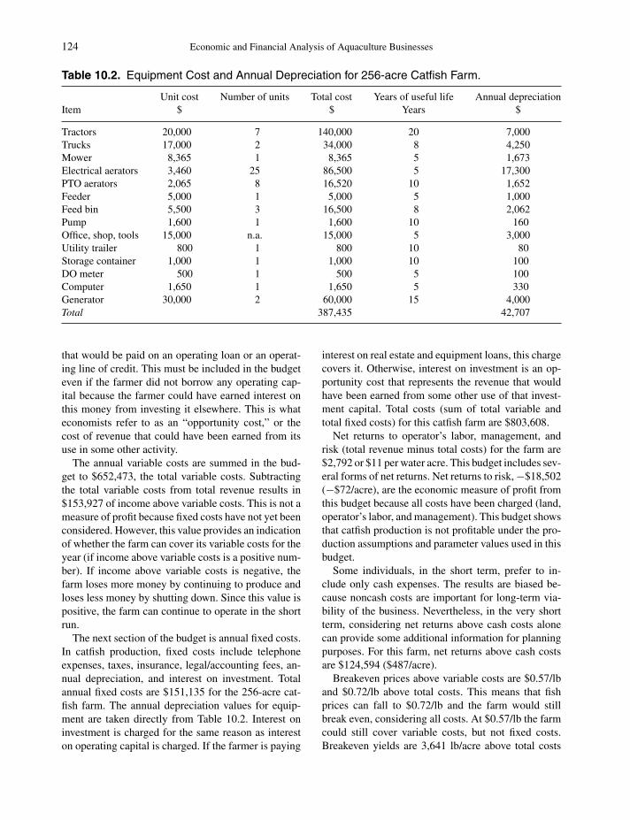
P1: SFK/UKS P2: SFK



Table 10.2. Equipment Cost and Annual Depreciation for 256-acre Catfish Farm.

Unit cost Number of units Total cost Years of useful life Annual depreciationItem $ $ Years $

Tractors 20,000 7 140,000 20 7,000Trucks 17,000 2 34,000 8 4,250Mower 8,365 1 8,365 5 1,673Electrical aerators 3,460 25 86,500 5 17,300PTO aerators 2,065 8 16,520 10 1,652Feeder 5,000 1 5,000 5 1,000Feed bin 5,500 3 16,500 8 2,062Pump 1,600 1 1,600 10 160Office, shop, tools 15,000 n.a. 15,000 5 3,000Utility trailer 800 1 800 10 80Storage container 1,000 1 1,000 10 100DO meter 500 1 500 5 100Computer 1,650 1 1,650 5 330Generator 30,000 2 60,000 15 4,000Total 387,435 42,707

that would be paid on an operating loan or an operat-ing line of credit. This must be included in the budgeteven if the farmer did not borrow any operating cap-ital because the farmer could have earned interest onthis money from investing it elsewhere. This is whateconomists refer to as an “opportunity cost,” or thecost of revenue that could have been earned from itsuse in some other activity.

The annual variable costs are summed in the bud-get to $652,473, the total variable costs. Subtractingthe total variable costs from total revenue results in$153,927 of income above variable costs. This is not ameasure of profit because fixed costs have not yet beenconsidered. However, this value provides an indicationof whether the farm can cover its variable costs for theyear (if income above variable costs is a positive num-ber). If income above variable costs is negative, thefarm loses more money by continuing to produce andloses less money by shutting down. Since this value ispositive, the farm can continue to operate in the shortrun.

The next section of the budget is annual fixed costs.In catfish production, fixed costs include telephoneexpenses, taxes, insurance, legal/accounting fees, an-nual depreciation, and interest on investment. Totalannual fixed costs are $151,135 for the 256-acre cat-fish farm. The annual depreciation values for equip-ment are taken directly from Table 10.2. Interest oninvestment is charged for the same reason as intereston operating capital is charged. If the farmer is paying

interest on real estate and equipment loans, this chargecovers it. Otherwise, interest on investment is an op-portunity cost that represents the revenue that wouldhave been earned from some other use of that invest-ment capital. Total costs (sum of total variable andtotal fixed costs) for this catfish farm are $803,608.

Net returns to operator’s labor, management, andrisk (total revenue minus total costs) for the farm are$2,792 or $11 per water acre. This budget includes sev-eral forms of net returns. Net returns to risk, −$18,502(−$72/acre), are the economic measure of profit fromthis budget because all costs have been charged (land,operator’s labor, and management). This budget showsthat catfish production is not profitable under the pro-duction assumptions and parameter values used in thisbudget.

Some individuals, in the short term, prefer to in-clude only cash expenses. The results are biased be-cause noncash costs are important for long-term via-bility of the business. Nevertheless, in the very shortterm, considering net returns above cash costs alonecan provide some additional information for planningpurposes. For this farm, net returns above cash costsare $124,594 ($487/acre).

Breakeven prices above variable costs are $0.57/lband $0.72/lb above total costs. This means that fishprices can fall to $0.72/lb and the farm would stillbreak even, considering all costs. At $0.57/lb the farmcould still cover variable costs, but not fixed costs.Breakeven yields are 3,641 lb/acre above total costs

P1: SFK/UKS P2: SFK



Table 10.3. Annual Costs and Returns for a 256-acre Catfish Farm (Stocking 5,690 5-inchFingerlings/acre; Feed Fed at 4.78 tons/acre/year; Yield of 4,500 lb/acre; Fingerlings PurchasedOff Farm; Pond Owned by Farmers).


Gross receipts Catfish foodfish lb 1,152,000 0.70 806,400Variable costs

Feed 32% protein floating Ton 1,223.68 227.4 278,265Fingerlings 5-inch Inch 7,283,200 0.010 72,832Labor Year-round, full-time FTE∗ 2 20,280 40,560

Seasonal or part-time FTE 0.5 20,280 10,140Plankton control Empirical average Acre 256 14.40 3,686Gas and diesel Empirical average Acre 256 130 33,280Electricity Empirical average Acre 256 289 73,984Repairs and maint. Empirical average Acre 256 97 24,832Bird depredation supplies Acre 256 6.25 1,600Seining and hauling Catfish foodfish lb 1,152,000 0.05 57,600Telephone Empirical average Acre 256 10.50 2,688Office supplies Empirical average Acre 256 11.00 2,816Interest on operating capital $ 501,902† 0.10 50,190

Total variable costs Per farm 652,473Per acre 2,549

Income above variable costsper farm

153,927

Fixed costsFarm insurance Empirical average Acre 256 25.3 6,477Legal/accounting Empirical average Acre 256 6.1 1,562Investment

Land Empirical average $ 210,432‡ 0.1 21,043Wells Empirical average $ 48,000§ 0.1 4,800Pond construction Empirical average $ 357,888¶ 0.1 35,789Equipment Empirical average $ 387,570 0.1 38,757

Annual depreciationEquipment Empirical average Acre 1 42,707 42,707

Total fixed costs Per farm 151,135Per acre 590

Total costs Per farm 803,608Per acre 3,139

Net returns to operator’slabor, management, and riskper farm

2,792

Per acre 11Opportunity costs

Operator’s labor Family Each 1 10,140Operator’s management Family Each 1 11,154Total opportunity costs of

family labor and management21,294

Total costs 824,902

(Continued)

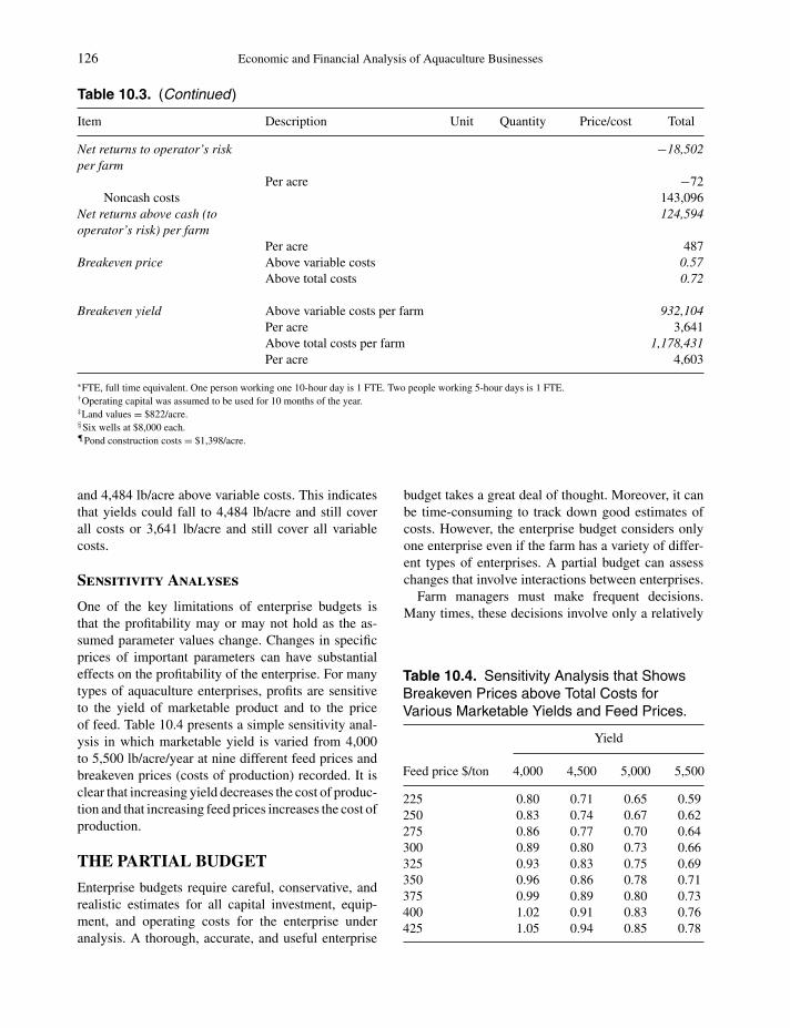
P1: SFK/UKS P2: SFK



Table 10.3. (Continued)


Net returns to operator’s riskper farm

−18,502

Per acre −72Noncash costs 143,096

Net returns above cash (tooperator’s risk) per farm

124,594

Per acre 487Breakeven price Above variable costs 0.57

Above total costs 0.72

Breakeven yield Above variable costs per farm 932,104Per acre 3,641Above total costs per farm 1,178,431Per acre 4,603

∗FTE, full time equivalent. One person working one 10-hour day is 1 FTE. Two people working 5-hour days is 1 FTE.†Operating capital was assumed to be used for 10 months of the year.‡Land values = $822/acre.§Six wells at $8,000 each.¶Pond construction costs = $1,398/acre.

and 4,484 lb/acre above variable costs. This indicatesthat yields could fall to 4,484 lb/acre and still coverall costs or 3,641 lb/acre and still cover all variablecosts.

Sensitivity Analyses

One of the key limitations of enterprise budgets isthat the profitability may or may not hold as the as-sumed parameter values change. Changes in specificprices of important parameters can have substantialeffects on the profitability of the enterprise. For manytypes of aquaculture enterprises, profits are sensitiveto the yield of marketable product and to the priceof feed. Table 10.4 presents a simple sensitivity anal-ysis in which marketable yield is varied from 4,000to 5,500 lb/acre/year at nine different feed prices andbreakeven prices (costs of production) recorded. It isclear that increasing yield decreases the cost of produc-tion and that increasing feed prices increases the cost ofproduction.

THE PARTIAL BUDGET

Enterprise budgets require careful, conservative, andrealistic estimates for all capital investment, equip-ment, and operating costs for the enterprise underanalysis. A thorough, accurate, and useful enterprise

budget takes a great deal of thought. Moreover, it canbe time-consuming to track down good estimates ofcosts. However, the enterprise budget considers onlyone enterprise even if the farm has a variety of differ-ent types of enterprises. A partial budget can assesschanges that involve interactions between enterprises.

Farm managers must make frequent decisions.Many times, these decisions involve only a relatively

Table 10.4. Sensitivity Analysis that ShowsBreakeven Prices above Total Costs forVarious Marketable Yields and Feed Prices.

Yield

Feed price $/ton 4,000 4,500 5,000 5,500

225 0.80 0.71 0.65 0.59250 0.83 0.74 0.67 0.62275 0.86 0.77 0.70 0.64300 0.89 0.80 0.73 0.66325 0.93 0.83 0.75 0.69350 0.96 0.86 0.78 0.71375 0.99 0.89 0.80 0.73400 1.02 0.91 0.83 0.76425 1.05 0.94 0.85 0.78

P1: SFK/UKS P2: SFK



small change in its operation (e.g., changing the stock-ing rate, adding a pond with a different species, addinga fingerling pond). If the change is a relatively smallone, the majority of costs across the enterprise willremain the same with and without the change. Thesechanges could be evaluated by comparing two whole-farm budgets, but this can consume time that is notwarranted by the small size of the change.

A partial budget is an analytical technique designedto evaluate the effect of the changes in benefits, costs,and net returns from making such a small change inthe farm operation. A partial budget is a standardizedand formal method to calculate the change in profitfrom a possible change. It is important to note thata partial budget does not mean arbitrarily choosingsome but not other costs. In a partial budget analysis,all changes in costs and benefits must be considered,but the analysis considers only the changes that willoccur.

A partial budget answers the following question:what will be the net economic effect on the farm frommaking a relatively small change to the operation?A partial budget analysis is limited in that it can beused to analyze only two alternatives at a time. Thesetypically include the current situation as the base andone proposed alternative. Different partial budgets areneeded to analyze a series of changes. Partial budgetsare useful for existing enterprises that are consideringa management change. This might consist of changingstocking densities and stocking sizes, increasing theaeration level, changing to a different type of feed, orbeginning to buy fry to produce fingerlings on farm.However, partial budgets can also be used to consideradding investment items such as whether to purchasean in-pond fish grader, add a hatchery building to thefish enterprise, or purchase new aerators. A partialbudget is not appropriate for a new enterprise for whichcomprehensive estimates of the costs and benefits donot exist.

The bottom line of the partial budget is called thechange in net benefit. This is the measure of whethernet returns would increase or decrease by making theproposed change and by how much. If the change innet benefit is positive, then making this change on thefarm will increase net returns. However, if negative,then the change considered would reduce net returns.The magnitude of the values indicates the extent of thechange.

The unit of analysis for a partial budget should bethe same as for the enterprise budget that serves as thebasis for the analysis. If the unit of the base enterprise

budget is one 10-acre pond, then the partial budgetshould be for a 10-acre pond. However, if the baseenterprise budget is for an entire farm, then the partialbudget should be for the entire farm.

The two broad categories that form the frameworkof the partial budget are the benefits and costs thatresult from the proposed change. All items that areexpected to change are allocated to the appropriatecategory.

The benefits include additional revenue and reducedcosts, while costs include reduced revenue and addi-tional costs. Additional revenue can result if the pro-posed change results in higher levels of marketableyield or if the change would add a new species thatwould generate new revenue. The additional revenuecategory includes the revenue to be earned if thechange is adopted on the farm. However, the analy-sis includes new revenue that is not being earned inthe current situation. Additional revenue often resultsfrom increased yields, sales from a new enterprise,gaining a higher price, or increasing the size of theenterprise.

Benefits from the change also result from reductionof costs on the farm. Switching to a cheaper feed, re-ducing the size of the farm, or eliminating a fingerlingoperation would reduce costs. For example, if perhapsa new feed resulted in an improved feed conversion,the quantity of feed fed for a given level of marketableyield would be reduced and total feed costs wouldbe lower. The cost category includes any reduction inrevenue from the farm. Reduced revenue representsrevenue currently earned that would not be availableafter the change is made. A lower price, reduced salesfrom lower yields or fewer production acres, or elimi-nation of an enterprise would reduce revenue. Anotherexample would be the revenue lost of one species byswitching to a different species.

The cost category also includes the new, additionalcosts associated with the alternative being consideredthat are not part of the current costs. Higher stockingand feeding rates, purchasing new fingerlings, buyingadditional ponds for expansion or for raising a newspecies will all be new costs. Examples of additionalcosts would be if the new feed or fingerlings consideredcost more.

Once all the changes have been itemized and quan-tified, the additional revenues are added to the reducedcosts to obtain the benefits. Reduced revenue is addedto additional costs to obtain the costs. Costs are sub-tracted from benefits to obtain the change in net bene-fits.

P1: SFK/UKS P2: SFK



Other Considerations in DevelopingPartial Budgets

Opportunity costs must also be considered in partialbudgets. Additional variable costs require capital thatcould be invested elsewhere and that value is includedas an additional cost. On the other hand, reduced vari-able costs also represent an opportunity cost that nolonger exists.

Sensitivity analyses should be done on key param-eters to evaluate how dependent the results are onchanging values for important parameters. Sensitiv-ity analyses are conducted by varying the price of theparameter in consistent increments and measuring thechange in the net benefits.

Partial budgets are a simple and easy way to evaluatemanagement changes. The data required are usuallyminimal. However, it can only compare one change ata time. A partial budget is not well suited to analyze achange where the revenues are not constant from yearto year. Typical partial budgets also do not account forrisk; yet, changes in risks as a result of the change canbe important and should be evaluated.

RECORD-KEEPING FORENTERPRISE AND PARTIALBUDGETS

Records are fundamental to the development of en-terprise and partial budgets. For an enterprise bud-get, records must be maintained on yields, typicallyin lb/acre or kg/ha for ponds, lb or kg/m3 for cagesor tank systems, and lb or kg/gallon of water flow forraceways. Sales records must be maintained. Recordsof purchase of supplies, including fingerlings, feed,fuel, and repairs and maintenance are necessary.

Labor records must be maintained, divided intosalaried personnel and hourly workers. Benefits pro-vided to salaried personnel must be itemized. This mayinclude use of pickup truck for personal use, housingprovided on the farm, or other benefits. Hourly workersneed to be itemized by full-time seasonal or part-timeworkers.

It is best, if possible, to maintain records of the hoursof use of machinery. This is particularly useful fortractors and aerators. Purchase and sale of equipmentas well as service records need to be maintained.

Practical Application of a PartialBudget

Table 10.5 illustrates the application of a partial bud-get to the 256-acre catfish farm situation. The change

Table 10.5. Partial Budget of Adding a HybridStriped Bass Enterprise (40 acre) on a256-acre Catfish Farm.

Category Value or cost

BenefitsAdditional revenue

40 acres in hybrid striped bassproduction, producing 4,500lb/acre/year, at $1.50/lb

$270,000

Reduced costs$3,139/acre for catfish costs, for40 acre

$125,560

Total Benefits $359,560Costs

Additional costsFeed: 191.2 tons for 40 acre,$50/ton more for feed

$9,560

Fingerlings: $0.20/fingerling $45,520Interest on operating capital $4,590Marketing $75,000

Reduced revenue40 acres at 4,500 lb/acre catfish ×$0.70/lb

$126,000

Total Additional Costs $260,670Net Benefit $98,890

being considered is to take 40 acres of water currentlyin catfish production and stock those acres with hybridstriped bass for foodfish growout.

Additional revenue would consist of the sales ofhybrid striped bass foodfish. Sales were estimated tobe based on 40 acres in production, with a yield of4,500 lb/acre/day, at a price of $1.50/lb, for additionalrevenue of $270,000 (Table 10.5). Costs would bereduced for the catfish no longer raised in those 40acres of water. Because Table 10.3 shows total costsof $3,139/acre for catfish production on this size offarm, the reduced costs would be $125,560 for the40 acres taken out of production. Total net benefits(sum of additional revenue and reduced costs) are$395,560.

Hybrid striped bass fingerlings are more expensivethan channel catfish fingerlings, and the feed for hy-brid striped bass is also more expensive. Moreover,because hybrid striped bass are sold either live or onice, there would be additional marketing costs esti-mated at $75,000. The catfish not sold from these 40acres constitute reduced revenue of $126,000. The totaladditional costs (sum of additional costs and reducedrevenue) are $386,228. The net benefit from switching

P1: SFK/UKS P2: SFK



40 acres from catfish to hybrid striped bass is $98,890.Because this number is positive, the analysis demon-strates that the change is feasible. However, it shouldbe noted that this analysis has not considered addi-tional risks associated with producing and marketinghybrid striped bass.


Dey et al. (2005) used field survey data collected bythe WorldFish Center and partners to develop esti-mates of net returns for a variety of production systems,species, and production technologies. Net returns wereestimated for seven different countries (Bangladesh,China, India, Indonesia, Philippines, Thailand, andVietnam). Species analyzed included carps, tilapia,prawns, snakehead, and walking and striped catfish.Production systems included cages and ponds stockedin both mono- and polyculture.

The analysis indicated that fish farming of freshwa-ter species in the selected Asian countries was gener-ally profitable. Profits tended to be higher with mono-culture of higher-valued carnivorous species such asprawns, snakehead, and walking catfish. However,resource-poor fish farmers could also raise omnivo-rous and herbivorous species profitably in both mono-and polyculture. Semi-intensive levels of productionwere shown to produce higher rates of return thanvery extensive or intensive production levels. The ex-tensive production technologies were inefficient in thatresources were underutilized while the very intensiveproduction systems had much higher costs of variableinputs.

SUMMARY

This chapter provided a detailed description of enter-prise and partial budgets. These budgeting tools pro-vide a mechanism to assess whether or not a proposedenterprise is profitable, how profitable it is expected tobe (enterprise budget), and whether a proposed changeon the farm is expected to be profitable (partial bud-get). Care must be taken to include all relevant costsand to use conservative estimates of all cost and rev-enue items. Prices expected to be received must bebased on long-run averages as should be the costs ofvarious input items.

Sensitivity analyses should be run on all parametersfor which values are either unknown or those that arehighly variable. Breakeven analysis further shows the

prices and quantities that will need to be obtained tocover all costs.

REVIEW QUESTIONS

1. Explain how breakeven prices and yields can beused to determine the profitability of the enter-prise.

2. How do sensitivity analyses evaluate the risk ofthe enterprise?

3. What would be an appropriate unit of analysis foran enterprise budget for a trout raceway farm?

4. What would be the greatest single cost for each ofthe following aquaculture enterprises:a. Salmon netpen farmb. Trout raceway farmc. Subsistence tilapia pond farmd. Shrimp pond production farm

5. Describe alternative ways to assign a value tosubmarketable-sized fish in a pond.

6. List the major limitations to an enterprise bud-get analysis and how its interpretation should beproperly qualified.

7. Explain why there is a charge for interest on op-erating capital in an enterprise budget.

8. Explain the difference between net returns to oper-ator’s labor, management, and risk and net returnsto risk.

9. What advice would you give someone when theenterprise budget shows positive income abovevariable costs but negative net returns?

10. Explain what types of employee charges would beproperly charged as fixed costs and which wouldbe categorized as variable costs.

REFERENCES

Dey, Madan M., Mohammad A. Rab, FerdinandJ. Paraguas, Ramachandra Bhatta, Mohammad F.Alam, Sonny Koeshendrajana, and MahfuzuddinAhmed. 2005. Status and economics of freshwater

P1: SFK/UKS P2: SFK



aquaculture in selected countries of Asia. Aquacul-ture Economics and Management 9:11–37.

Engle, Carole R. 2007. Arkansas Catfish ProductionBudgets. Cooperative Extension Program MP 466.Pine Bluff, AR: University of Arkansas.

Kay, Ronald D., William M. Edwards, and Patricia A.Duffy. 2008. Farm Management. Sixth Ed. Boston:McGraw-Hill.

National Agricultural Statistics Service, U.S. Depart-ment of Agriculture. www.usda.mannlib.cornell.edu/MannUSDA/viewDocumentInfo.do?documentID=1375. Accessed November 13, 2009.

United States Bureau of Labor Statistics. www.bls.gov. Accessed November 13, 2009.

United States Department of Energy. www.eia.doe.gov. Accessed November 13, 2009.

P1: SFK/UKS P2: SFK


11Financial Statements: Balance Sheet

and Income Statement in Aquaculture

Financial management and control of a business forefficient operation requires regular and periodic doc-umentation and review of financial performance andprogress. The purpose of financial analysis is to iden-tify problems and opportunities, potential solutions,and then develop plans to take advantage of the op-portunities. It summarizes the financial position andcondition of the business at a specific point in time.The two main instruments used for periodic financialmanagement and control are the balance sheet and theincome statement. This chapter explains what each ofthese instruments is, how each is structured, and whateach tells the financial analyst or farm owner.

The balance sheet is a financial statement that item-izes assets and liabilities for the business and calculatesnet worth as its bottom line. Net worth measures thelevel of wealth of the business while the relationship ofthe assets to the liabilities provides a clear view of thefinancial position of the business. Financial positionrefers to the total amount of resources that a businesscontrols as well as the financial claims against thoseresources. Many lenders consider the balance sheet tobe the most important financial statement of all be-cause it can be used to determine whether the businessor individual can tolerate additional debt.

The income statement measures the revenue andexpenses of the business for the specified time period.An income statement resembles an enterprise budgetand is sometimes confused with it. The difference be-tween the two is that the enterprise budget is devel-oped for a typical, average, generalized farm businesswhile the income statement is developed for a specificbusiness for a specified time period, typically, a year.

Thus, the income statement documents the financialperformance of the business for that particular year,but not for the average conditions facing an industry.The income statement measures the profit or loss forthe business for that particular year and is also knownas a profit and loss statement.

Many financial transactions affect both the balancesheet and the income statement, and some values nec-essary from the income statement are obtained from thebalance sheet. Thus, it is essential that balance sheetsand income statements be prepared for the same timeperiod and at the same time. They must be interpretedtogether for a thorough understanding of business per-formance. Any time that revenue and expenses change,the balance sheet and income statements may change.Accurate interpretation of these financial statementsrequires that the time period of analysis be specifiedbecause revenue and expenses are different for differ-ent time periods.

The greatest value of the balance sheet and incomestatement is derived from using them over time tointerpret the overall financial performance and positionof the business. From year to year, a viable businesswill show a generally increasing net worth from thebalance sheet and increasing net farm income from theincome statement.

THE BALANCE SHEET

The balance sheet is a key financial statement usedby businesses to monitor financial performance andprogress. It is also called the statement of financialcondition. The balance sheet measures the financialposition of the business for that specific time period.It organizes all that is owned by the business (assets)and the debts that are owed (liabilities) in a systematic


131

P1: SFK/UKS P2: SFK



manner and is prepared for a given point in time. Ifalways prepared at the same time each year, the balancesheet can be used to compare the financial progress ofthe business from year to year and the growth of thebusiness can be charted over time.

The bottom line of the balance sheet is net worth.Net worth is also referred to as owner’s equity and mea-sures the level of capital that the owners have investedin the firm. Assets, liabilities, and owner equity are in-terrelated and “balanced” in the balance sheet. Ownerequity is the difference between assets and liabilities.This relationship can be expressed mathematically as:

Net worth (owner equity) = assets − liabilities

This same relationship can be expressed as:

Assets = owner equity + liabilities

Over time, a successful business is one in which thenet worth increases over time. Increases in net worthmean that the owner is accumulating wealth from thebusiness.

The balance sheet is developed for the entire farmbusiness for the fiscal year used by the business. Itcan be developed to show the capital position at anytime, but the most useful balance sheets are developedannually, corresponding to the beginning and ending ofthe financial year. The ending balance sheet of any oneyear is identical to the beginning balance sheet for thenext year. Balance sheets commonly are prepared forthe end of the calendar year, as of December 31. Thisstatement then serves as both the end-of-year statementfor that year and the beginning statement for the nextyear (January 1).

Careful thought should be given to the choice offinancial accounting periods. The fiscal year can bethe calendar year or it can be some other period oftime. The calendar year is convenient from a financialperspective because many people prepare their incometaxes for the calendar year. This is also a time whenmany farms located in temperate areas have time to an-alyze their finances carefully. However, other financialaccounting periods can be used. There is some advan-tage to matching the production year with the financialreporting year. For a catfish farm, for example, finger-lings typically are stocked in February or March. Aprilis one of the first good feeding months. Thus, usinga financial reporting year of April through March ofthe following year tracks the production cycle moreclosely. Fish produced that year typically are soldover the winter months and revenue can be matchedmore closely to expenses when the financial account-

ing period is aligned closely with the production cycle.Alternatively, some farmers maintain financial recordsdeveloped for both reporting periods.

Regardless of the financial accounting period se-lected, the balance sheet should be developed at leastonce a year to be able to monitor financial progressover time. The same time period should be used overthe years to maintain consistent accounting practices.Any changes observed, then, will be due to changingfinancial position of the business and not an artifactof the accounting system. Managers may want to ex-amine quarterly balance sheets to more closely mon-itor the financial position of the business. This maybe especially important during difficult financial andeconomic times.

The structure of the balance sheet includes majorcategories of “assets” and “liabilities.” All assets andliabilities for the firm are listed on the balance sheet.Assets include anything that is owned by the businesswhile liabilities are the value of debts owed by the busi-ness. Any item of value that is owned by the businessis considered an asset. Items are considered as assetsif they have a value either because they can be sold togenerate cash revenue or because they can be used toproduce something else that will be sold at a later time.All debts and financial obligations owed to someoneelse constitute liabilities. Liabilities represent a claimby someone else, an outside entity, on the assets of thebusiness.

Assets and liabilities are further divided into sub-categories referred to as “current” and “noncurrent”assets and liabilities and refer to the period of timewithin which the specific asset or liability will be used.These classifications are based on what is termed “liq-uidity.” Liquidity is the extent to which an asset cangenerate cash quickly and efficiently to meet the busi-ness’s financial commitments. Highly liquid assets arethose that can be converted to cash with little or no de-lay or loss in the net value of the firm. Current assetsare those that are highly liquid and include assets thatare expected to be converted into cash (sold) withina period of 1 year. In other words, current assets areshort-term liquid assets.

For example, inventories of catfish that are expectedto be sold within a year would be categorized as acurrent asset while equipment such as tractors and aer-ators would be classified as noncurrent assets. Currentassets include the value of raw materials and supplieson the farm at the time the balance sheet is developed.Stocks of herbicides, copper sulfate, feed, or other in-puts should be included. These types of current assets

P1: SFK/UKS P2: SFK


Financial Statements: Balance Sheet and Income Statement in Aquaculture 133

typically are valued at their original purchase cost.Assets commonly included as current assets are cashon hand and balances in checking and savings ac-counts. These clearly are very liquid types of assets.Accounts receivable (payments not yet received fromprocessing plants for fish already delivered) can alsobe important current assets.

Any asset that is expected to be used in the busi-ness for more than a year is classified as a noncurrentasset. Noncurrent assets typically have a useful lifegreater than 1 year, are usually not purchased for re-sale, and are used to produce products or services thatwill be sold. Noncurrent assets typically are those thatthe business owns because they are used to produce theproducts sold to generate revenue. Thus, equipment,broodstock, ponds, and land are classified as noncur-rent assets. If aerators or tractors would be sold, thefish farm would likely not be able to produce and sellas much product in the future. These noncurrent assetsare less liquid (illiquid). They are more difficult to sellquickly and easily at full market value. Broodstock areanother example of a noncurrent asset because brood-stock are generally considered to be fixed assets. Be-cause broodstock frequently are produced on farm ormay have been purchased some time ago, assigninga value can be more difficult. Broodstock can be val-ued at: (1) cost of production; (2) 75% of reasonablemarket cost; or (3) anticipated market value after de-ducting storage, transportation, and marketing costs.The most common way to assign a value to brood-stock is the anticipated market value. Costs associatedwith storage and transportation need to be subtractedout.

Estimating the inventory of aquatic crops can be dif-ficult, depending on the production system. Net pens,cages, tanks, and raceways are more amenable to fre-quent inventory estimations than open-pond systems.Estimating the quantity of fish available in a 10-acrepond that has been in continuous production for manyyears is difficult. For many species, there is no veryaccurate and precise manner to obtain such an inven-tory estimate. Errors in the estimate of the inventorycan create errors in the balance sheet and income state-ments. Experienced farmers with excellent records willhave better estimates of the quantity and sizes of fishin the pond.

Current liabilities are short-term debt obligations.Current liabilities include debt-servicing payments duewithin the year and accounts payable to feed mills orsupply companies. Short-term loans require completepayment of principal and interest within 1 year. Those

payments due within the coming year are classified ascurrent liabilities.

Noncurrent liabilities consist of the remaining bal-ances on loans (other than the current year’s payments)and other financial obligations that will be incurred ata point in time later than the current year. These in-clude operating loans and lines of credit. Loans takenout for the purchase of noncurrent assets, such as land,pond construction, and equipment, will typically haveterms of lending of more than 5 years (see Chapter14 for more details on commonly used types of loansfor aquaculture). Thus, payments on principal and in-terest due are made over a period of years. The re-maining balance of principal on the loans is classifiedas a noncurrent liability. When calculating noncurrentliabilities, it is important to be certain to deduct thepayments due in the coming year. The payments duein the coming year are listed as current liabilities, andneed to be subtracted from the noncurrent liabilities.

On the balance sheet, the values of the current as-sets are summed; the values of the noncurrent assetsare also summed. The total value of the current assetsis then summed with the total value of the noncurrentassets to obtain total assets. Similarly, all the valuesof the current liabilities are summed to obtain “totalcurrent liabilities” and the values of the noncurrentliabilities are summed to obtain “total noncurrent lia-bilities.” Total current liabilities are added to the totalnoncurrent liabilities to obtain “total liabilities.”

Net worth is calculated on the balance sheet by sub-tracting the total value of all liabilities from the totalvalue of all assets of the business (total assets − totalliabilities). Net worth is also referred to as owner eq-uity. It is the amount of money left for the owner of thebusiness if the business were to be sold and all liabili-ties paid in full. Net worth (owner equity) is consideredto be a claim on the assets by the owner(s) of the busi-ness. Owner equity changes over time. The goal of thebusiness is for net worth to increase over time.

Profits generated by the business are used to paydown liabilities and increase net worth as liabilitiesdecrease. Alternatively, if profits are used to acquireadditional assets, net worth will increase if the totalamount of liabilities remains constant. However, networth will also change if the value of an asset changes.Thus, if land values decline, the total value of assetswill decline. For fish farm balance sheets, the valueof the swimming inventory can be a substantial por-tion of current assets. If fish prices decline, currentassets will go down in proportion to the decline infish prices. It should be noted that if assets increase

P1: SFK/UKS P2: SFK



but are financed through a loan, the liabilities will in-crease by the same amount as the increase in assets.In such a case, net worth will remain the same. Networth changes when the owner puts additional per-sonal capital into the business, withdraws capital fromthe business, or the business shows as a profit or loss.

Notes on Valuing Assets

There are two principal methods for assigning a valueto assets: cost-basis or market-basis. The cost basisvalue is also referred to as the “book value.” Basicaccounting principles specify use of a cost basis. Witha cost basis, assets are valued using the cost, cost lessdepreciation, or farm production cost methods. Theadvantage of a cost-based balance sheet is that it isdirectly comparable to other balance sheets preparedwith standard accounting principles and is a conserva-tive estimation method. Moreover, the net worth willnot vary because of market fluctuations. The advan-tage of a market-based valuation approach is that itmore accurately indicates the value of collateral andthe current financial position of the business.

Typically, depreciable assets are valued as cost lessdepreciation. Submarketable fish and broodstock typ-ically are valued at farm production cost. Inventoriesof market-sized fish, however, are valued at marketprice even on a cost-based balance sheet. The differ-ence between the cost basis and market basis valuesis typically larger for assets purchased several yearsbefore the preparation of the financial statement. Forexample, the current market value of ponds may bevery different from the original construction cost 20years ago. The balance sheet should indicate the basisof accounting (cash- or market-based), the nature ofthe operation (number of ponds, acres), and the depre-ciation method used.

Record-Keeping for theBalance Sheet

Records required to prepare a balance sheet includecomplete inventories of both current and noncurrentassets. A spreadsheet can be used to itemize all check-ing and savings accounts for the business. The year-endbalance in each serves as the beginning value for thenext year’s pro forma balance sheet.

To be able to prepare a balance sheet, the farm busi-ness must maintain records of all assets and liabilities.The farm should maintain a table or spreadsheet thatincludes line items for land and each building on thefarm. For land, the current value per acre for similarland in that area should be recorded, along with the

number of acres and the total value. Each buildingshould be listed separately, with the original purchaseprice or construction cost, the estimated years of use-ful life, the annual depreciation, and the current value.Similarly, there should be a separate table or spread-sheet that includes each equipment item for the farm,its initial purchase price, the estimated years of usefullife, the annual depreciation, and the current value.

Farm records should include a depreciation schedulefor all the equipment on the farm. This table shouldinclude the original purchase price, the date of theoriginal purchase, the depreciation method used (i.e.,straight-line, double-declining balance), the estimatedyears of useful life, and the current value.

A similar schedule should be maintained for theponds, tanks, grading sheds, office, and other buildingson the farm. This table should also include columnsto record the original purchase price, the date of theoriginal purchase, the depreciation method used (i.e.,straight-line, double-declining balance, etc.), the esti-mated years of useful life, and the current value.

Additional tables are needed to maintain records ofthe inventory of the aquatic crops and of materials andsupplies in hand at the beginning of the year and atthe end of the year. The inventory sheet for aquaticcrops should list these by species and by size groupper pond. The estimated inventory of fish should in-clude an estimate of the quantity of fish in each pondby size group of fish. This can be estimated from aFishy file (Fishy is a record-keeping software programused in the U.S. catfish industry.) (Killcreas 2009), bysampling, or by careful examination of the stocking,feeding, and harvesting records for the farm. The esti-mated number and individual weight of each should berecorded along with the total value. Market-sized fishor shrimp should be valued at the market price whilesubmarketable fish or shrimp should be valued at theestimated production cost.

Supplies on hand and their total value (purchasecost) at the beginning and end of the year should alsobe itemized with total quantities recorded. The changein value for each (crops and supplies) is calculated forlater use in the income statement.

Each farm business should maintain careful recordsof loans. A table or spreadsheet should be main-tained that includes the following information for eachyear:

1. Initial and ending dates of loan2. Dates when payments due3. Amount of payment, separated into interest and

principal portions

P1: SFK/UKS P2: SFK



4. Balance remaining on the principal at the end offinancial period

These should be updated annually.

Practical Application: 256-acreCatfish Farm

Table 11.1 presents an example of a balance sheetfor the 256-acre catfish farm described in Chapter 10.Assets are listed first and then liabilities. Assets and li-abilities are shown in order of liquidity. In other words,the more liquid assets (current assets) are listed first.The current assets include the cash available in thefarm business ($15,849). The cash available consistsof cash on deposit in a bank account. In addition tothe cash available, there is an inventory of catfish inthe ponds that is expected to reach market size andbe sold during the current year. There are 4,500 sub-marketable fish/acre (based on 75% survival of the

Table 11.1. Balance Sheet for a 256-acreCatfish Farm, December 31.

Item Total value


Cash on deposit $15,849Checking account balance 0Accounts receivable 0Fish inventory∗ $266,112

Total current assets $281,9612. Noncurrent assets

Equipment $387,570Ponds $357,888Wells $48,000Land $210,432

Total noncurrent assets $1,003,8903. Total assets $1,285,851Liabilities4. Current liabilities

Payments on debt due andpayable over next yearEquipment $72,368Real estate $38,216


Equipment loan $168,858Real estate loan $254,772

Total noncurrent liabilities $423,6306. Total liabilities $534,2147. Net worth (3–6) $751,637

*4,500 submarketable fish/acre at 0.33 lb each @ $0.70/lb.

6,000/acre fingerlings stocked). At 0.33 lb each and aprice of $0.70/lb, the total value of fish in inventoryis $266,112. Total current assets for the 256-acre farmare $281,961.

Noncurrent assets for the 256-acre catfish farm in-clude equipment and farm real estate, including theland and ponds constructed on the land as well asthe necessary wells. The total value of the equipmentis $387,570, the ponds are valued at $357,888, thewells at $48,000, and the total land value is $210,432.The total value of noncurrent assets is $1,003,890. To-tal assets (sum of current and noncurrent assets) are$1,285,851.

On the liabilities side of the balance sheet, currentliabilities are listed first. Current liabilities include thepayments due over the next year for the catfish farm.The catfish farm has loans for equipment and real estateand, thus, has payments due over the course of theyear. The equipment loan payment for the current yearis $72,368 and the real estate loan payment for thecurrent year is $38,216. Total current liabilities are$110,584.

Noncurrent liabilities include the value of the prin-cipal that remains to be paid on the equipment andpond construction loans. The remaining principal onthe equipment loan is $168,858 and the remainingprincipal on the pond construction loan is $254,772.Total noncurrent liabilities are $423,630. Total liabil-ities (sum of current and noncurrent liabilities) are$534,214.

Total owner equity (net worth) (total assets − totalliabilities) for the 256-acre catfish farm is $751,637.Over time, the net worth should increase as the liabili-ties decrease and assets increase through equity gainedwith payments of principal.

INCOME STATEMENT

The income statement is a companion financial state-ment to the balance sheet and is also key to moni-tor financial performance and progress. The incomestatement measures the profit or loss generated by thebusiness for the specific time period used for finan-cial analyses. It summarizes the financial transactionsthat affect revenue and expenses for the period of timespecified in the income statement and measures thedifference between revenue and expenses. Thus, itsprimary value is to determine whether the businesswas profitable for that time period, but it can alsobe used to monitor profits from one year to the next.Moreover, it can also be used to identify what portionof profits is generated from different resources used in

P1: SFK/UKS P2: SFK



the production process. (For more detail, see Chapter4 on monitoring economic and financial performanceof aquaculture businesses.)

The bottom line of the income statement is net farmincome from operations. This indicator shows whetherthe farm business resulted in a profit or loss for thatparticular year. If net farm income is positive, then thefarm was profitable that year, and if net farm incomeis negative, then it suffered losses.

The income statement is calculated for the sametime period as the balance sheet. Complete financialanalysis requires that both these statements be calcu-lated at the same time and for the same time period.The income statement and balance sheets should beprepared at least annually. However, some managersmay wish to examine quarterly statements to keep acloser eye on the business, especially during difficultfinancial times.

The structure of the income statement is somewhatsimilar to that of an enterprise budget. The primarydifference is that the income statement includes rev-enue and expenses actually incurred over the time pe-riod specified whereas the enterprise budget includeslong-run average revenue and expenses. Other differ-ences are that the income statement sorts out interestexpenses from the other expenses.

The first category in the income statement is rev-enue. All revenue received by the farm business overthe past financial period is included in the income state-ment and is itemized by the source of revenue. Thus,the value of sales of foodfish for the past year wouldbe included in the revenue category of the annual in-come statement. If the farm also sold fingerlings, thesewould be indicated on a separate line. Any governmentpayments received (such as disaster payments) wouldalso be included in this area. Revenue that results fromthe sale of a capital asset such as land or another pieceof equipment is also included as revenue. However,for a capital asset, the value entered into the incomestatement is the difference between the price the assetis sold for and the initial cost of purchase. Revenueresulting from the sale of a depreciable asset, such asa tractor, is valued as the difference between the pricethe tractor is sold for and the initial cost of purchaseafter subtracting out the accumulated depreciation. Foraccrual-based income statements (see section on Cashversus Accrual-Based Income Statements), the changein value of the inventory of fish and inputs shouldalso be included in the revenue portion of the incomestatement. Any change in the accounts receivable (ac-counts receivable represent payments for product de-livered that have not yet been received) must also be

included. For example, if a fish or shrimp farmer de-livers a load of product to a processing plant, but hasnot yet received payment at the time of developingthe financial analysis, the value of that payment is an“account receivable.” These values are obtained fromthe differences in the beginning and ending balancesheets.

The next major category in the income statement isthat of cash farm expenses. Those operating expensesthat were paid during the accounting period, with theexception of interest payments, are itemized in thissection. Typically, the value of fingerlings, feed, andlabor are included in this category. Repair and util-ity bills paid and seining and hauling costs are alsoincluded. Payments on insurance and taxes are fixedcosts in an enterprise budget, but are cash operatingexpenses and listed as such in the income statement.The value of all the cash operating costs is summed toobtain total cash farm expenses.

Depreciation is a noncash cost and is included as aseparate line item in the income statement. The valueof depreciation is the sum of the loss in value forall depreciable assets for the financial accounting pe-riod being analyzed. Depreciation on all capital itemsshould be included, particularly equipment, ponds, andany buildings. Broodstock are frequently considered tobe fixed or capital assets. As fixed assets, the value ofbroodstock enters the income statement only as depre-ciation or net replacement cost.

Interest expenses are separated from other cash ex-penses. The Farm Financial Standards Council consid-ers interest expense a result of financing, not produc-tion activities. Thus, interest expenses are not includedwith the direct cash operating expenses of producingfish and other aquatic crops. Loan principal paymentsare not considered expenses because the capital bor-rowed is simply being returned to the original owner.The “payment” or cost is the interest paid. Thus, prin-cipal payments are not included in the income state-ment. (Note that the payment of the principal amountsof loans is an important financial consideration that istreated in Chapter 12 that discusses cash flow.) Theprincipal was an amount borrowed that does have tobe returned, but is not an expense.

However, the income statement includes depreci-ation costs to account for the replacement costs ofcapital goods. Including a principal payment on loansfor capital goods, in a sense, would “double count” thecost of acquiring/replacing capital goods.

Net farm income is the measure of profit or lossof the farm business. If net farm income is positive,then the farm business was profitable for that period of

P1: SFK/UKS P2: SFK



time; if negative, it lost money for that period of time.The Farm Financial Standards Council recommendsincluding income taxes in the income statement. Ifthis is done, net farm income becomes an after-tax netfarm income.

Cash versus Accrual-BasedIncome Statements

There are two fundamental accounting approachesused in agriculture: cash-based and accrual-basedaccounting. In cash-based accounting, revenue isrecorded when cash is received regardless of when theproduct was produced or the service provided. Thus,with cash accounting, revenue can be recorded in anaccounting period other than the one in which the prod-uct was produced. For example, if a crop of catfish isproduced in 2010, but fish were off-flavor and not solduntil 2011, then the revenue is recorded in the 2011 in-come statement if cash-based accounting proceduresare used.

Expenses similarly are recorded in the accountingperiod when they are paid, or when the cash is spentwith cash-based accounting. Items that are paid forlate in one year and not used until the next are chargedto the first year’s income statement. Alternatively, iffertilizer is charged to an account payable in 2010, butthe account payable is not paid until 2011, then theexpense is included in the 2011 income statement.

The advantage of the cash accounting method is thatit is simple and easily understood. It is also the mostcommonly used method in fish farming. The disad-vantage is that neither revenue nor expense is directlyrelated to the production obtained in the particularfinancial reporting year. Thus, the profit or loss esti-mated in the income statement does not truly representthe profit or loss from that particular year’s production.

The Farm Financial Standards Council recommendsthe use of accrual-based, not cash-based accounting. Inaccrual accounting, the value of products produced andservices provided are recorded for the year in whichproduced, regardless of when the cash revenue was ac-tually received or the expenses actually paid. There isno difference between cash-based and accrual-basedaccounting when all revenues are received and ex-penses incurred in the same year as that of the pro-duction that resulted. However, when revenues are re-ceived in the year following the one in which productsare produced, or expenses paid in a different year fromthe actual production, results of income statements de-veloped based on accrual accounting will differ fromthose obtained with cash-based accounting.

The major difference in the two methods lies in theway inventories are handled. In accrual accounting,the value of changes in inventories is expressed asrevenue in the income statement. For example, on acatfish farm, expenses for feed, fingerlings, utilities,and labor are incurred throughout the production year.However, if the fish are off-flavor at the end of the year,there will be no revenue that year. Cash revenue willbe received the next year when the catfish come backon-flavor, are sold, and revenue received. In accrual ac-counting, the value of the catfish produced is includedas revenue in the year during which the productionoccurred. The way this is handled in the accrual-basedincome statement is to add a line in the revenue sectionfor the change in inventory of fish. The fish producedthat year but not sold are measured by the increase intotal weight of fish in the ponds over the course of theyear. This increase in the weight of fish on the farm isrecorded as a positive change in the inventory. Becausethese are market-sized fish, the value used would bethe market price.

Expenses in accrual-based accounting are handledin a similar fashion. Those expenses incurred in pro-ducing the revenue in that year are recorded in thatsame year. If supplies are purchased and paid for in thesame year, the expense section of the income statementwill be the same for cash-based and accrual-based ac-counting statements. However, if items are purchaseda year before that when revenue is produced or are notpaid for until the year after they are used, then the re-sults will be different for cash-based and accrual-basedaccounting. If not yet paid for, these enter the accrual-based income statement as a change in inventory. Ifinterest is accrued in one year but the cash payment isnot due for several more months, differences will beincurred.

The main advantage of accrual-based accountingis that it provides a more accurate estimate of profit.The information provided for financial analysis andmanagement is more accurate. The disadvantage isthat accrual accounting procedures are more difficultand require more time. Also, accrual accounting maynot be the most beneficial for income tax reporting.The Farm Financial Standards Council recommendsthat anyone using cash-based accounting should alsocalculate an accrual-adjusted net farm income.

Record-Keeping for theIncome Statement

Farms must maintain adequate records from whichthe income statement is calculated. Basic records for

P1: SFK/UKS P2: SFK



revenue required for the income statement begin withthe delivery tickets from the processing plant. Thetickets from the plant will itemize whether dockageswere incurred due to: (1) out-of-size fish; (2) diseasedand deformed finfish; (3) dead-on-arrival fish; (4) trashfish; or (5) some other reason. This ticket will providenumbers for the weight and number of fish delivered,as well as the losses suffered due to dockages. The netprice received can also be recorded after adjusting forthe dockages charged.

Purchases of supplies typically involve: (1) obtain-ing a price quotation; (2) placement of an order; (3)delivery bill; (4) receipt of invoice or bill; (5) receipt ofstatement of account at end of month; and (6) receiptsfor payments made. Thus, the records available arethe delivery ticket, invoice, monthly statement, andcanceled check for payment. These records can bechecked for accuracy or errors by comparing: (1) theorder against the invoice; (2) the invoice against the de-livery ticket; and (3) the delivery ticket against goodssupplied.

Practical Application: 256-acreCatfish Farm

Table 11.2 illustrates an income statement for the 256-acre catfish farm. The farm sold 1,152,000 lb of food-sized catfish. At $0.70/lb, the total revenue for the yearis $806,400.

Cash operating expenses include those costs listedas variable costs on the enterprise budget as wellas cash expenses of legal/accounting fees and in-surance costs that are listed as “fixed costs” onthe enterprise budget. These operating expenses in-clude feed ($278,265), fingerlings ($72,832), labor($40,560 for a full-time year-round employee and$10,140 for seasonal, part-time labor), plankton con-trol ($3,686), gas, diesel fuel, and oil ($33,280), elec-tricity ($73,984), repairs and maintenance ($24,832),bird depredation supplies ($1,600), seining and haul-ing costs ($57,600), telephone ($2,688), office supplies($2,816), legal/accounting fees ($1,562), and insur-ance expenses ($6,477). Total cash farm expenses sumto $610,322.

Depreciation costs for losses in value of equipmentand buildings for this farm for the year totaled $42,707.This value is added to total cash farm expenses toobtain total catfish farm expenses of $653,029.

Interest paid is placed under a separate category inthe income statement. This facilitates calculation offinancial ratios that are described in Chapter 4. On the

Table 11.2. Income Statement for a 256-acreCatfish Farm, December 31.

Item Total value

Catfish farm revenueCash catfish sales $806,400Accounts receivable 0Change in market livestock inventory 0

Total catfish farm revenue $806,400Catfish farm expenses

Cash operating expensesFeed $278,265Fingerlings $72,832Labor $40,560

$10,140Plankton control $3,686Gas, fuel, and oil $33,280Electricity $73,984Repairs and maintenance $24,832Bird depredation supplies $1,600Seining and hauling $57,600Telephone $2,688Office supplies $2,816Legal/accounting $1,562Insurance $6,477

Total cash farm expenses $610,322Accounts payable 0Prepaid expenses 0Depreciation $42,707

Total operating expenses $653,029Cash interest paidInterest on operating line of credit $50,190Interest paid on long-term loans

Land $21,043Wells $4,800Pond construction $35,789Equipment $38,757

Total interest paid $150,579Total expenses $803,608Net farm income from operations $2,792

256-acre catfish farm, there are loans for the operat-ing capital as well as long-term loans for the land,wells, pond construction, and equipment. Annual in-terest payment on the operating line of credit for thisfarm is $50,190 and annual interest payments on thelong-term loans are $21,043 for the loan used to pur-chase the land, $4,800 for the loan used to dig thewells, $35,789 for the loan used to pay for construc-tion of the ponds, and $38,757 on the equipment loan.All interest expenses are summed to obtain a total ofthe cash interest paid ($150,579). This is added to the

P1: SFK/UKS P2: SFK



total catfish farm expenses to obtain total expenses forthe year of $803,608.

Net farm income from operations is calculated bysubtracting total expenses from total farm revenue, or$2,792 for the 256-acre catfish farm. Thus, the farmgenerated a profit for the year, even though the totalamount of profit was not great.

Practical Application: Cash versusAccrual Accounting

Tables 11.3 and 11.4 compare cost-based and accrual-based income statements for the farm situation pre-sented in Table 11.2, but with one difference. In Table11.2, all the catfish produced in 2010 were sold in2010, and all expenses for the 2010 crop were paidfor in 2010. Thus, there is no difference in the incomestatement regardless of whether the farm used cash-based or accrual-based accounting.

Farms rarely are able to sell all their fish by Decem-ber. Off-flavor or market conditions typically resultin only part of the fish produced being sold in thatsame year. Tables 11.3 and 11.4 present income state-ments showing the profit or loss for the farm if only50% of the catfish produced are sold in 2010. Table11.3 uses cash-based accounting and Table 11.4 usesaccrual-based accounting. Both tables show results forthe years 2010 and 2011.

With cash-based accounting, when the farm sellsonly 50% of its 2010 crop in 2010, the revenue is half($403,200) (Table 11.3) of what it was when all fishwere sold in 2010 ($806,400) (Table 11.2). This re-sults in a negative net farm income from operations in2010 of −$400,408. In 2011, assuming that all the off-flavor fish of 2010 were sold as they came on-flavorfrom January to March, and the 2011 crop was all soldin 2011, the revenue in 2011 would be $1,209,600.This is much higher than that shown in Table 11.2 andresults in a higher net farm income from operationsof $405,992. Imagine a banker looking at the 2010 in-come statement; he or she would see a substantial losson the farm and might begin to question the financialviability of the business.

In the accrual-based income statement in Table 11.4,the increase in the weight of catfish on the farm overthe 2010 production season is recorded as a changein inventory. The market-sized inventory that was pro-duced but not sold is valued at its market price. Actualsales in 2010 were 50% of the sales shown in Table11.2 because only 50% of the fish were sold. Thus,

the total farm revenue for 2010 was $806,400. This isequal to the revenue shown in Table 11.2.

The accrual-based income statement for 2011 shownin Table 11.4 shows increased cash sales of catfish,because the market-sized catfish from 2010 were soldin addition to the 2011 crop. However, at the end of2011, because the 2011 crop was all sold, there wouldbe a decrease in the total weight of fish on the farm(as compared to the beginning of the year). Thus, thechange in inventory line item under revenue shows adecreased value of inventory on the farm. Total revenuefor 2011, then, is the same as in 2010, and net farmincome from operations is the same as in 2010. Thebanker reviewing this farm’s financial statements seesa consistently profitable business. The profits may below, but it is a business that is making all its paymentsand is a viable operation.

The examples shown in Tables 11.3 and 11.4 weresimplified to illustrate the differences in cash-basedand accrual-based accounting. For a real business, cat-fish prices would not likely be constant from year toyear nor would expenses. The proportion of market-sized fish not sold in December is likewise not con-stant and varies with a number of factors. Never-theless, these examples show the benefit of usingaccrual-based accounting. If the farm uses cash-basedaccounting for income tax purposes, then an accrual-adjusted statement should also be developed. The dif-ficulties of estimating inventories in open-pond sys-tems were noted earlier in the chapter. Nevertheless,well-managed farms must strive to maintain adequaterecords and estimates of fish inventories.

RELATIONSHIP BETWEEN THEBALANCE SHEET AND THE INCOMESTATEMENT

The balance sheet and the income statement are re-lated. For example, for the balance sheet to show in-creasing net worth over time, the business must gen-erate profits. Thus, the profit or loss measured by theincome statement will affect the financial position ofthe business, as measured by the balance sheet. Con-sistent losses from year to year will make it difficultto make loan payments, will affect crop inventories onthe farm, or may require the sale of capital assets thatreduce the total value of assets to the business.

Changes in values from the beginning and endingbalance sheets for livestock, broodstock, and accountsreceivable are entered directly into the revenue sectionof the income statement. Changes in supplies, prepaid

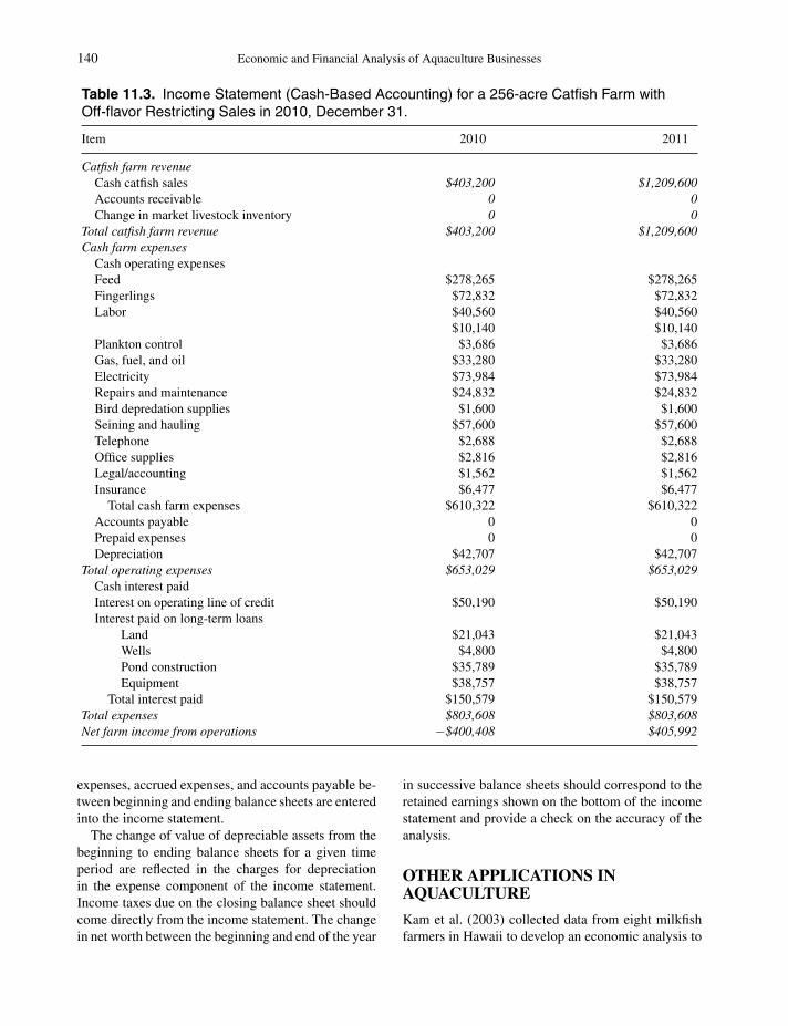
P1: SFK/UKS P2: SFK



Table 11.3. Income Statement (Cash-Based Accounting) for a 256-acre Catfish Farm withOff-flavor Restricting Sales in 2010, December 31.

Item 2010 2011

Catfish farm revenueCash catfish sales $403,200 $1,209,600Accounts receivable 0 0Change in market livestock inventory 0 0

Total catfish farm revenue $403,200 $1,209,600Cash farm expenses

Cash operating expensesFeed $278,265 $278,265Fingerlings $72,832 $72,832Labor $40,560 $40,560

$10,140 $10,140Plankton control $3,686 $3,686Gas, fuel, and oil $33,280 $33,280Electricity $73,984 $73,984Repairs and maintenance $24,832 $24,832Bird depredation supplies $1,600 $1,600Seining and hauling $57,600 $57,600Telephone $2,688 $2,688Office supplies $2,816 $2,816Legal/accounting $1,562 $1,562Insurance $6,477 $6,477

Total cash farm expenses $610,322 $610,322Accounts payable 0 0Prepaid expenses 0 0Depreciation $42,707 $42,707

Total operating expenses $653,029 $653,029Cash interest paidInterest on operating line of credit $50,190 $50,190Interest paid on long-term loans

Land $21,043 $21,043Wells $4,800 $4,800Pond construction $35,789 $35,789Equipment $38,757 $38,757

Total interest paid $150,579 $150,579Total expenses $803,608 $803,608Net farm income from operations −$400,408 $405,992

expenses, accrued expenses, and accounts payable be-tween beginning and ending balance sheets are enteredinto the income statement.

The change of value of depreciable assets from thebeginning to ending balance sheets for a given timeperiod are reflected in the charges for depreciationin the expense component of the income statement.Income taxes due on the closing balance sheet shouldcome directly from the income statement. The changein net worth between the beginning and end of the year

in successive balance sheets should correspond to theretained earnings shown on the bottom of the incomestatement and provide a check on the accuracy of theanalysis.


Kam et al. (2003) collected data from eight milkfishfarmers in Hawaii to develop an economic analysis to

P1: SFK/UKS P2: SFK



Table 11.4. Income Statement (Accrual-Based Accounting) for a 256-acre Catfish Farm withOff-flavor Restrictions on Sales in 2010.

Item 2010 2011

Catfish farm revenue 2010 2011Cash catfish sales 403200 1209600Accounts receivable 0 0Change in market livestock inventory $403,200 −$403,200

Total catfish farm revenue $806,400 $806,400Cash farm expenses

Cash operating expensesFeed $278,265 $278,265Fingerlings $72,832 $72,832Labor $40,560 $40,560

$10,140 $10,140Plankton control $3,686 $3,686Gas, fuel, and oil $33,280 $33,280Electricity $73,984 $73,984Repairs and maintenance $24,832 $24,832Bird depredation supplies $1,600 $1,600Seining and hauling $57,600 $57,600Telephone $2,688 $2,688Office supplies $2,816 $2,816Legal/accounting $1,562 $1,562Insurance $6,477 $6,477

Total cash farm expenses $610,322 $610,322Accounts payable 0 0Prepaid expenses 0 0Depreciation $42,707 $42,707

Total operating expenses $653,029 $653,029Cash interest paidInterest on operating line of credit $50,190 $50,190Interest paid on long-term loans

Land $21,043 $21,043Wells $4,800 $4,800Pond construction $35,789 $35,789Equipment $38,757 $38,757

Total cash interest paid $150,579 $150,579Total expenses $803,608 $803,608Net farm income from operations $2,792 $2,792

assess the feasibility of growing milkfish to a smallermarket size and of extensive culture of milkfish inHawaii. Income statements were developed for eachscenario evaluated to measure and compare profitabil-ity. Sensitivity analyses were conducted to evaluate theeffects on profits of varying levels of the price of milk-fish, yield (kg/ha), labor cost, feed prices, and stockingcosts.

The income statements indicated that the optionsconsidered were not economically feasible for milkfish

as a startup business. Further analyses indicated thatreducing the share of costs allocated to the milkfishenterprise on the farm will result in positive returns.

SUMMARY

This chapter described balance sheet and income state-ment, two of the most important financial statementsused to analyze the financial performance of a busi-ness. The chapter explained how the net worth that is

P1: SFK/UKS P2: SFK



calculated from the balance sheet measures the wealththat is being accumulated in the business. The chap-ter also explained how the income statement measuresthe profit or loss for that particular year. The struc-ture and mechanics of each of these statements is ex-plained and practical applications summarized. Issuesrelated to valuation of assets, cash-based and accrual-based accounting, and the relationship between the twostatements are discussed. Finally, the records requiredto develop balance sheets and income statements aredescribed.

REVIEW QUESTIONS

1. Explain what information is obtained from thebalance sheet.

2. Explain what information is obtained from theincome statement.

3. What is the difference between an enterprise bud-get and an income statement?

4. What is the difference between cash-based andaccrual-based accounting?

5. How are the balance sheet and income statementsrelated?

6. What are the difficulties posed by many aquacul-ture systems in the use of accrual-based account-ing?

7. What is net worth and how can it be used to ana-lyze an aquaculture business?

8. What is the difference between current liabilitiesand noncurrent liabilities?

9. For real estate loans, how are the payments appor-tioned between current and noncurrent liabilitieson the balance sheet?

10. What is the primary indicator calculated on the in-come statement and how can it be used to evaluatethe farm business?

REFERENCES

Kam, Lotus E., Francisco J. Martınez-Cordero, Ping-Sun Leung, and Anthony C. Ostrowski. 2003. Eco-nomics of milkfish (Chanos chanos) production inHawaii. Aquaculture Economics and Management7(1/2):95–123.

Killcreas, Wallace E. 2009. Fishy 2009, Version 10.0.Stoneville, MS: Mississippi State University.

P1: SFK/UKS P2: SFK


12Cash Flow Analyses in Aquaculture

INTRODUCTION

Most aquaculture businesses are capital-intensive fromthe perspective of both short-term and long-term capi-tal. Few aquatic farmers have sufficient capital of theirown to meet the financial needs of the business. Thus,most farmers borrow capital for short- and long-termcapital needs. Short-term capital needs refer to the op-erating capital needed to purchase feed, fingerlings,fuel, and other operating inputs while long-term cap-ital is required to purchase land, build ponds, andbuy equipment. Careful management of these loansrequires that close attention be paid to the flow of cashand how the cash flow pattern in the business affectsthe ability to make loan payments required to servicethe debt in an adequate manner.

A key consideration in the cash flow budget is thetiming of receipt of cash and the timing of expendituresof cash. A critical component of a cash flow analysisis to identify when cash is expected to be receivedand when it is expected to be spent. Thus, the cashflow budget is a unique type of financial instrument;no other financial statement accounts for the timing ofthe amounts of cash coming in and going out of thebusiness.

Cash flow analysis results in a picture of the move-ment of cash into and out of the business. It representson paper how much cash is available at the beginning ofthe planning period, when cash will flow into the busi-ness from what sources and at what level, and whencash will leave the business for which purposes andin what quantity. Finally, the analysis will show howmuch cash will be left at the end of the planning period.

The bottom line of the cash flow budget is the cashavailable for each unit of time included in the analy-sis. The cash available shows whether there is enough

cash inflow to the business to cover all expenses tobe incurred in the business for that particular time pe-riod. For example, for a monthly cash flow budget,the cash available for each month shows whether thereis enough to meet the expenses anticipated in eachmonth. If the value for that month is negative, thenadditional operating funds must be either taken fromsavings or borrowed from a lender to obtain sufficientcash needed for that month to make the payments. Thischapter explains the importance of cash flow analysisand the difference between cash flow statements andbudgets, describes the structure and mechanics of each,and explains its interpretation.

CASH FLOW STATEMENTS VERSUSCASH FLOW BUDGETS

The terminology related to cash flow analysis differsdepending on whether the analysis is done with recordsfrom the past year or if it is used to project cash flowinto the future. If the analysis is done with records fromthe past year, it is referred to as a cash flow statement,or a statement of cash flow. If the analysis projectscash revenue and expenses into the future, it is a cashflow budget, sometimes also referred to as a pro formacash flow budget.

IMPORTANCE OF CASH FLOWANALYSIS

Cash flow analysis is one of the most useful financialanalyses. The balance sheet, income statement, andcash flow analysis combine to provide the fundamentalset of financial analyses necessary for understandingthe basic financial condition of a business.

One of the most serious financial problems facedby farmers is the control of cash flow. Cash needs areoften greater than the amount of cash available dur-ing the production season. Sales often tend to occur ingroups and do not flow into the farm business evenly


143

P1: SFK/UKS P2: SFK



throughout the year. Many of the receipts from salesoccur after production has taken place, following com-plete harvest of the crop. Such a seasonal pattern ofcash inflow creates cash deficits that cause farmers todraw down savings accounts or to borrow additionalfunds to cover the deficits.

The availability of cash to make necessary paymentsis as important as profitability to the economic feasibil-ity of a business. Adequate cash flow is a key compo-nent of the financial feasibility of a business. Positivecash flow can often make the difference between suc-cess and failure of an aquaculture business, especiallyin the early years of a business startup.

The cash flow budget is a critical component of anynew business plan (see Chapter 3 for more detail ondeveloping business plans). It serves as a useful toolfor determining the most appropriate time to replacecapital assets like aerators or tractors, or to renovateand rebuild ponds. Cash flow budgets can be used toidentify the best schedule to make larger, more discre-tionary purchases of new capital, insurance premiums,or others that can be planned out over time. Exten-sive cash flow planning may identify opportunities topurchase inputs at discounts, or through more detailedincome tax planning.

The cash flow budget is used to evaluate the needfor new borrowing. It provides critical insights intowhether the business will have adequate cash avail-able when needed to meet its financial obligations.The time periods that exhibit a shortfall in cash arethose in which additional new borrowing is needed.The amount of the cash shortfall is the amount that isneeded.

A cash flow budget can be used to develop a borrow-ing and debt repayment plan. Such a plan can preventexcessive borrowing and provide guidance as to thebest way to pay down debt quickly. Cash flow budgetsare used to develop accurate lines of credit that ensurecash will be available when needed to meet financialobligations.

The cash flow analysis shows whether new loans arefeasible and whether there will be cash when needed tomake payments on any new loans. Businesses need ad-equate amounts of capital, but careful attention needsto be paid to the ability of the business to make thenecessary payments. If the terms of lending requirepayments in excess of what the business will havecash for, the business may fail.

Lenders use cash flow budgets to assess thechances of receiving scheduled payments on time fromprospective new borrowers. It is a key component in aproper business loan proposal because it shows directly

how and when borrowed capital (especially short-termoperating loans) will be repaid.

WHAT A CASH FLOW BUDGETIS NOT

Cash flow statements and budgets measure cash flowand cash position, not profits in the business. Cash flowand position are extremely important components ofan overall financial analysis of a business, but do notmeasure profit. Profit for a particular time period ismeasured by the income statement; enterprise budgetsindicate profit in a generalized way for a typical year.The difference is that income statements and enter-prise budgets include noncash costs such as depreci-ation, while cash flow analysis considers movementsof cash only. Noncash costs must be included in thecalculation of profit because if a business cannot gen-erate enough revenue to replace its equipment when itwears out (cover its noncash depreciation costs), it isnot profitable over the longer term and it will not sur-vive. Noncash revenue and expenses are not includedin the cash flow budget; so, it does not measure profit,only cash position.

This does not mean that cash flow and position arenot important; these areas are as important as the in-formation provided by the other financial statements.For example, a business that shows losses on the in-come statement for a period of time can survive andrecover. However, a business that has inadequate cashresources and cannot pay its bills will not last long. Onthe other hand, having a positive cash flow by itself isnot enough to ensure that a business will be profitableand successful. To fully evaluate the business requiresbalance sheets and income statements in addition tocash flow statements and budgets.

STRUCTURE AND MECHANICS OFTHE CASH FLOW BUDGET

The cash flow budget should be developed for the sameenterprise unit as the balance sheet and income state-ment. If the entire business is for one enterprise, forexample, catfish, then the cash flow budget should bedeveloped for the entire farm, as is the case for thebalance sheet and income statement.

One of the basic premises of adequate cash flowin a business is that the bills must be paid on time; inother words, there must be cash available when neededto make the payments. If cash revenue in a particularmonth is less than the cash expenses, then money mustbe borrowed to pay the bills. However, if there is a cash

P1: SFK/UKS P2: SFK


Cash Flow Analyses in Aquaculture 145

surplus in one time period, that surplus can roll overto the next time period to be used to make paymentsthat are due later in the year. Or, if not needed for otherpayments that will become due, it can be used to makeadditional payments on the principal of a loan to payit off more quickly and reduce the interest charges.Alternatively, the surplus could be deposited into asavings account or used to purchase other capital assetsthat might improve productivity of the farm business.Thus, the fundamental premise of cash flow budgetingis that the total cash received, regardless of whether it isreceived from the sale of product or made available byborrowing capital from a bank, must be at least equalto the total amount of expenses during that time period.

Cash flow budgets can be structured differently de-pending on the purpose for which the analysis is beingdeveloped. For detailed financial planning, monthlycash flow budgets are useful. Monthly cash flow bud-gets are primarily used to estimate the amount andtiming of additional borrowing needed to cover short-falls of cash in specific time periods, and to assess theability of the business to make the associated paymentson time. Monthly budgets for farm businesses are themost useful in agriculture because of the seasonal na-ture of most farming businesses. Monthly cash flowbudgets allow for development of a detailed analysisof the relationship of the timing and amounts of cashflowing into and out of the business. Quarterly budgetscan be used to develop estimates of cash flow needsover a several-year period. Annual cash flow budgetsare used in investment analyses to determine cash flowover the life of the investment. (see Chapter 13 onInvestment Analysis.)

For maximum benefit to the farm manager, it is bestto prepare an end-of-year statement of cash flows aspart of the financial analysis for the business. The state-ment of cash flows is a financial record that recordswhat happened in terms of cash flow over the pastyear. The statement of cash flows will show the pat-tern of cash flow over the past year and provides insightinto when payments will be needed for the upcomingyear. It will also show the time periods in which cashflow is likeliest to be a problem. The cash flow budgetis then developed for the upcoming year to project thefuture needs of the business, plan for new borrowing,and schedule payments to meet debt-servicing require-ments.

A cash flow budget summarizes and itemizes cashinflows (cash received into the business) and the cashoutflows for the business for the specific time periodanalyzed. There are certain key principles to keep inmind when constructing a cash flow budget. As trite

as it may seem, it is important to keep in mind thatonly cash inflows and outflows are considered. Nononcash revenue or noncash expenses are considered.For example, depreciation is not included in the cashflow budget, but the proceeds from sales of any capitalassets are included. Inventory values are not includedbut receipts from sales of product from inventory are.

Principal payments are not included in the incomestatement, but represent a cash outflow. Thus, pay-ments of both principal and interest are included inthe cash flow budget. A primary concern in the cashflow budget is the timing of receipt of revenue andexpenses. The cash flow budget is prepared by identi-fying the timing and magnitude of the expected cashflows into and out of the business. Each type of rev-enue or expense is charged during the specific periodwhen it is received or incurred. Thus, if a major capitalasset is purchased during a given period, its entire costis charged out in that time period in the cash flow bud-get. All cash received and expended must be identifiedand included in the appropriate time period in whichit is received and expended.

The cash flow budget is set up with columns thatrepresent specific time periods and rows that includespecific line items of cash inflow or outflow. A cashflow budget developed to make management decisionson the farm (typically, a monthly cash flow budget)would include each month in a column in the cashflow budget. The rows would include the specific rev-enue items, operating expenses, capital expenditures,and scheduled debt payments. The cash available iscalculated for each month. If the cash flow budgetis developed for an investment analysis, the columnswould be years instead of months.

The cash flow budget begins with the sources ofcash receipts that are expected to flow into the busi-ness. Cash receipts frequently include the cash balanceavailable at the beginning of the time period, cash rev-enue from sales of farm products sold, cash receivedfrom the sale of capital assets (land, equipment, brood-stock), and nonbusiness cash receipts from nonfarmcash income, cash gifts, and other sources of cash.

The beginning cash balance or the amount of cashon hand at the beginning of the period is listed first.The beginning cash amount is taken directly from thecurrent portion of the balance sheet for January 1.This is followed by each source of farm cash revenuegenerated by sales of the crop or of other capital assets.The cash revenue items are summed to generate totalcash inflow for the time period.

The easiest way to begin to complete the cash flowbudget is to create a total column on the far right of the

P1: SFK/UKS P2: SFK



budget. Annual totals for each line item are recordedin the total column. For example, the total amountof cash inflow from the sale of fish, shrimp, or crabsexpected for the coming year is recorded in the totalcolumn for the row of product sales for the business.This amount will be the same total value of revenue inthe enterprise budget and the total amount of revenuefrom product sales on the income statement. The nextstep is to apportion the amount of this revenue to bereceived for each month. The monthly amounts shouldadd up to the total listed in the total column for eachline item.

After cash receipts are itemized by time period,the same is done with cash outflows. Cash outflowstypically include farm operating expenses, cash out-flows from the purchase of any new capital assets(land, equipment, and broodstock), any nonbusinessexpenses such as living expenses, and payments ofprincipal and interest on outstanding loans.

Operating expenses are itemized first. Each typeof operating expense is listed. Thus, there is a rowfor feed expenses, fingerling costs, labor costs, utili-ties, etc. The total amount for the year is recorded inthe total column on the far right of the budget. Then,each month’s expense is recorded for the appropriatemonth. For example, catfish fingerlings typically arepurchased in February or March; fingerling expenseswould then be listed in either February or March as ap-propriate. The values of each type of cash outflow foreach time period should add to the amount listed in thetotal column. The amount in the total column shouldequal that in the enterprise budget and the income state-ment for each type of operating expense. Comparingthe sum of individual months with the amount listedin the total column is a good way to check for errorsin the accuracy of the budget.

The next section of cash outflow is to itemize theexpenses that result from the purchase of capital as-sets such as equipment or broodstock. Family livingexpenses frequently are included in the cash flow bud-get, particularly when it will be used for applying forloans from banks.

Payments of principal and interest for each loan areitemized in the subsequent section. All loan paymentsare included, for both current and noncurrent liabili-ties. It is best to itemize the payments by individualloan. This makes it easier to check the payments and tomake adjustments from year to year as the individualloans are paid off.

All expenses are summed to calculate total cashoutflow for each month. The difference between totalcash inflow and total cash outflow is the cash available,

sometimes called ending cash balance, for that partic-ular time period. If the cash available is negative, thismeans that there is insufficient cash generated duringthe period to meet all cash obligations and additionalborrowing is needed for that time period. After addingin the new borrowing, the cash balance is obtained. Ifthe cash available is a positive number for a particularmonth, then there is cash available that can be usedfor other purposes. An economical use of extra cash isto pay off the principal of existing loans, particularlythe operating capital loan. Paying off the principal asquickly as possible will minimize the total interest ex-penses paid. If not used to pay off loans, this cashamount can be carried over to subsequent time periodsfor upcoming cash needs in the coming months.

Cash balance becomes the beginning cash availableat the start of the next time period. The basic rule forcash balances is that the ending cash balance be at leastzero. That means that there is sufficient cash inflow tomeet the cash needs for that time period. However, azero ending cash balance also means that there is nocushion of cash for any unexpected problems or unan-ticipated expenses. It is prudent for the farm managerto plan for a certain amount of surplus cash to roll overfrom one time period to the next.

At the bottom of the cash flow budget, it is usefulto maintain an accounting of the debt outstanding foreach loan. Principal payments made in a time periodare subtracted out of the balance owed in the out-standing debt section. Maintaining an accounting ofoutstanding principal amounts on loans is not neces-sary for the cash flow budget, but it is a useful practice.It should be adjusted from month to month to reflectadditional payments on the principal as well as anynew borrowing. These lines of outstanding amountsof principal reflect the overall pattern of debt andhow it changes across the annual production cycleand patterns of cash flow. The lines of outstandingdebt on operating loans will also indicate whether thefarm is approaching any maximum limits on borrowedcapital.

COMPARISON OF CASH FLOWBUDGET WITH OTHER FINANCIALINSTRUMENTS

The cash flow budget represents a flow of cash overa period of time, unlike the balance sheet that repre-sents the financial position at one specific point in time.The income statement also represents a flow of incomeand expenses, but includes all revenue and expenses,not just cash revenue and expenses. The cash flow

P1: SFK/UKS P2: SFK



statement summarizes the year’s transactions and canhelp to reconcile net income calculated on an accrualbasis (see Chapter 11 for a discussion of accrual-based and cash-based accounting for income state-ments) with the change in cash position.

The cash flow budget contains all cash flows anddoes not contain any noncash revenue or noncash ex-penditures. Thus, what is included in a cash flow bud-get is distinct from the tabulation of revenue and ex-penses on the enterprise budget and income statement.The income statement includes noncash revenue likepositive changes in inventory whereas the cash flowbudget does not. Similarly, depreciation is included inan income statement as a noncash expense but becausedepreciation is not a cash expense, it is not includedin the cash flow budget. The total value of a new trac-tor (capital asset) purchased would not be included inthe income statement but is a negative cash flow in thecash flow budget because it is a cash outflow. Cash flowbudgets for farms frequently include cash outflow forpersonal expenses, because these may affect the cashavailable for the farm business; personal expenses arenot included in the income statement.

The cash flow budget does not indicate profit. Theincome statement is the measure of profit in the busi-ness. Because the cash flow budget does not includenoncash expenses, it does not measure profit. It onlymeasures the flow of cash. It is possible to have a largepositive cash flow and low profits from a business.This can occur when capital assets such as equipmentor land are sold. The cash proceeds are included as cashinflow, but may decrease profits because fewer cropscan be sold from less land. Similarly, it is possible tohave negative cash flow and a high profit. If new assets,such as new ponds, are built, or ponds are renovated,these cash expenses will decrease the cash available tothe business, but may result in greater profits from thesale of additional crops in the future.

Depreciation and changes in inventory values formany items are included in the income statement butdo not enter the cash flow budget. The cash flow bud-get contains several items that do not enter the incomestatement, such as the principal payments on debtsand capital expenditures. The income statement in-cludes all project expenses (whether paid or not) andthe value of items produced (whether sold for cash ornot). On the other hand, the cash flow budget identi-fies the amount and timing of all projected inflows andoutflows of cash.

Purchases of assets and loan activity are includedin cash flow statements and budgets but are not re-flected on the income statement, particularly if it is

accrual-based. This is because exchanging an asset fora different asset (selling a tractor to buy aerators) orexchanging an asset for a liability (selling an asset topay off a debt) do not constitute net income, but thesetypes of transactions do affect the cash position. Theincome statement is not adequate to show the effectsof these transactions on cash position, but the cashanalysis does reflect these effects.

The beginning cash of the cash flow budget is thevalue shown in the beginning balance sheet. Similarly,the ending cash position of the last period in the cashflow budget is the cash on hand for the projected year-end balance sheet. Projected capital sales and capitalpurchases from the cash flow budget supply the nec-essary information for determining the ending balancesheet values of capital assets. Information on loansoutstanding at the end of the year for the operatingline, intermediate-term loans, and long-term loans onthe pro forma balance sheet come directly from thecash flow budget.

RECORD-KEEPING FOR CASHFLOW BUDGETS

Inflows and outflows for the cash flow statement canbe taken directly from records of receipts and expen-ditures for each time period. A record-keeping systemfor cash analysis that has been used effectively is acash analysis book. In such a book, there is a col-umn to record a description of each transaction. Thisis followed by two additional columns, one to recordthe date of each transaction and the other to recordthe number of the check or receipt. Maintaining therecords in a looseleaf notebook provides flexibilityand individual sheets can be sent to the accountant.

It is best to have separate columns for receipts andpayments, as well as to separate capital receipts andcapital payments. The cash analysis book should beupdated at least once a month, to keep the receipts andexpenses current. The total for each category shouldbe added up each month.

Most cash in a business moves through the checkingaccount of the business. Thus, the checking accountstatements are a prime source of data for maintainingrecords for the cash flow budget.

The statement of cash flows is one of the finan-cial records that should be maintained by the business.Careful records of actual cash flows by month, byrecording and summarizing cash receipts and cash ex-penses each month provide a basis for comparison withthose budgeted for that month. This monthly compar-ison provides a basis for early identification of cash

P1: SFK/UKS P2: SFK



flow problems. This allows more time to search forsolutions and to make necessary changes.

Inventory records are necessary to develop the cashflow budget (see section on Record-Keeping for theBalance Sheet in Chapter 11). The estimates of inven-tory should include estimates of the quantity and valueof existing crops available for sale during that budgetperiod.

Records of outstanding loans, dates of scheduledpayments on each loan, and the amount to be chargedto principal and interest will be required.

PRACTICAL APPLICATION: CASHFLOW BUDGET FOR A 256-ACRECATFISH FARM

Table 12.1 presents a monthly cash flow budget forthe 256-acre catfish farm example used in previouschapters. Each month’s cash flow is listed as a sepa-rate column. Each line item (revenue or expense) isdescribed in the column to the far left. The column onthe far right has the total amount. The total amount foreach line item should correspond to the amount fromthe enterprise budget. This serves as a useful check onthe accuracy of the budget.

The first line category is revenue. The first itemlisted under revenue is the “beginning cash.” Begin-ning cash is the amount of cash that is available to thebusiness at the beginning of the time period. For theJanuary column, the beginning cash is what the farmerhas available to contribute to the farm business, oftenfrom a farm savings or checking account. In this ex-ample, the amount of beginning cash for the farm atthe beginning of January is $578,834.

The next line includes the sales of food-sized cat-fish, the only product sold by this farm business. Mostcash flow budgets include only the dollar value of theproducts sold by month, but for spreadsheets, it is of-ten easier to track if the actual weight is included asa separate line, as is done in Table 12.1. In this ex-ample, the farm sold 46,080 lb of catfish in January.The sales price was $0.70/lb and, thus, the revenue re-ceived in January from sales of food-sized catfish was$32,256. The revenue from sales of catfish foodfishis then added to the amount of beginning cash to ob-tain the total cash inflow for that month, in this case,$611,090 for January.

The next major heading in the cash flow budget isoperating cash expenses. Each type of expense is item-ized in a separate row. These rows should correspond tothe line items in the enterprise budget and in the income

statement. Thus, there are separate rows for feed, fin-gerlings, labor, plankton control, gas, diesel fuel, andoil, electricity, repairs and maintenance expenses, birddepredation costs, seining and hauling charges, tele-phone expenses, office supplies, farm insurance, andlegal/accounting fees. The expected cost of each ofthese that is anticipated to occur in that month is listedin the appropriate row. There are few feeding days inJanuary for channel catfish, and so only $2,783 is ex-pected to be spent on feed that month. Fingerlings arenot planned to be stocked until February and March;thus, there is no charge in January for the purchase offingerlings. The farm hires two people year-round whofeed and check night-time levels of dissolved oxygenduring the summer and spend most of their time scaringbirds and repairing equipment over the winter. Becausethey work fairly constant hours across the year, theirsalary cost is constant. The farm also hires some sea-sonal or part-time labor over the summer months, sothose charges do not appear in the cash flow budget un-til May and run through September. Plankton controlexpenses are not incurred until the summer months,either, with no charge in January. Gas, diesel fuel, oilcharges, electricity costs, and repairs and maintenanceexpenses are incurred to some degree over the wintermonths, but all increase during the primary productionperiod of May through October. On the other hand, birddepredation costs are incurred over the winter monthswhen the migratory birds are resting and feeding oncatfish ponds. Seining and hauling costs are incurredin the months when catfish are sold. Because they arecharged by the pound of fish sold, this cost can belinked to the pounds of fish sold in each month. Costsof the telephone, office supplies, farm insurance, andlegal/accounting fees occur in each month throughoutthe year.

When the operating expenses are completelyrecorded by line item for the month of January, theseare summed to obtain total monthly cash expenses. Forthe month of January, these total to $14,940. This is thetotal amount of cash that is needed to pay the expensesthat will be incurred in January.

The next category of items is the debt servicinglines. It is easier to manage and interpret the cash flowbudget if each loan is listed separately on the cash flowbudget, under the categories of real estate, equipment,and operating capital. It is also useful to separate theprincipal payments for each loan on a separate linefrom the interest payments. In Table 12.1, this farmdoes not have any loans (see Table 12.2 for a cashflow budget with debt-servicing payments) and, thus,

P1: SFK/UKS P2: SFK


Tab

le12

.1.

Mon

thly

Cas

hF

low

Bud

getf

ora

256-

acre

Cat

fish

Farm

with

outF

inan

cing

.

Item

Janu

ary

Febr

uary

Mar

chA

pril

May

June

July

Aug

ust

Sept

embe

rO

ctob

erN

ovem

ber

Dec

embe

rTo

tal

Beg

inni

ngca

sh57

8,83

459

6,15

057

7,54

855

7,82

366

4,92

171

3,61

472

7,08

970

4,96

770

2,06

369

8,54

479

0,83

482

4,53

8Po

unds

ofca

tfish

sold

,lb

46,0

8046

,080

46,0

8020

7,36

011

5,20

011

5,20

069

,120

115,

200

115,

200

195,

840

80,6

400

1,15

2,00

0

Rec

eipt

sfr

omca

tfish

sold

,$32

,256

32,2

5632

,256

145,

152

80,6

4080

,640

48,3

8480

,640

80,6

4013

7,08

856

,448

080

6,40

0

Tota

lcas

hin

flow

611,

090

628,

406

609,

804

702,

975

745,

561

794,

254

775,

473

785,

607

782,

703

835,

632

847,

282

824,

538

8,94

3,32

5

Ope

rati

ngca

shex

pens

esFe

ed2,

783

5,56

55,

565

19,4

7913

,913

44,5

2244

,522

55,6

5355

,653

16,6

968,

348

5,56

527

8,26

4Fi

nger

lings

036

,416

36,4

160

00

00

00

00

72,8

32L

abor

0Y

ear-

roun

d,fu

ll-tim

e3,

245

3,24

53,

245

3,24

53,

245

3,24

53,

650

3,24

53,

650

3,24

53,

650

3,65

040

,560

Seas

onal

,fu

ll-tim

e0

00

01,

521

2,53

52,

535

2,53

51,

014

00

010

,140

Plan

kton

cont

rol

00

00

922

092

20

1,84

30

00

3,68

7G

as,d

iese

lfue

l,an

doi

l1,

137

568

568

568

947

1,51

62,

463

2,46

33,

031

3,03

11,

326

1,32

618

,944

Ele

ctri

city

1,13

71,

137

1,70

52,

273

2,84

25,

683

8,52

59,

661

9,66

19,

661

2,84

21,

705

56,8

32R

epai

rsan

dm

aint

enan

ce2,

980

497

993

993

1,24

22,

483

3,22

83,

228

2,48

31,

242

1,24

24,

221

24,8

32

Bir

dde

pred

atio

n24

024

024

016

080

00

00

160

240

240

1,60

0Se

inin

gan

dha

ulin

g2,

304

2,30

42,

304

10,3

685,

760

5,76

03,

456

5,76

05,

760

9,79

24,

032

057

,600

Tele

phon

e21

521

516

126

926

921

521

521

521

521

521

526

92,

688

Offi

cesu

pplie

s22

528

141

5656

356

328

214

114

111

314

142

22,

816

Farm

insu

ranc

e51

851

851

851

851

851

858

351

858

351

858

358

36,

476

Leg

al/

acco

untin

g15

612

512

512

512

512

512

512

512

512

512

515

61,

562

Tota

lope

ratin

gex

pens

es14

,940

50,8

5851

,981

38,0

5431

,947

67,1

6570

,506

83,5

4484

,159

44,7

9822

,744

18,1

3757

8.83

3

Deb

tser

vici

ng

(Con

tinu

ed)

P1: SFK/UKS P2: SFK


Tab

le12

.1.

(Con

tinue

d)

Item

Janu

ary

Febr

uary

Mar

chA

pril

May

June

July

Aug

ust

Sept

embe

rO

ctob

erN

ovem

ber

Dec

embe

rTo

tal

Rea

lest

ate

Inte

rest

00

00

00

00

00

00

0Pr

inci

pal

00

00

00

00

00

00

0Su

btot

al0

00

00

00

00

00

00

Equ

ipm

ent

Inte

rest

00

00

00

00

00

00

0Pr

inci

pal

00

00

00

00

00

00

0Su

btot

al0

00

00

00

00

00

00

Ope

ratin

gIn

tere

st0

00

00

00

00

00

00

Prin

cipa

l0

00

00

00

00

00

00

Subt

otal

00

00

00

00

00

00

0To

tald

ebt

serv

icin

g0

00

00

00

00

00

00

Tota

lcas

hou

tflow

14,9

4050

,858

51,9

8138

,054

31,9

4767

,165

70,5

0683

,544

84,1

5944

,798

22,7

4418

,137

Cas

hav

aila

ble

596,

150

577,

548

557,

823

664,

921

713,

614

727,

089

704,

967

702,

063

698,

544

790,

834

824,

538

806,

401

New

borr

owin

g0

00

00

00

00

00

0

End

ing

cash

bala

nce

596,

150

577,

548

557,

823

664,

921

713,

614

727,

089

704,

967

702,

063

698,

544

790,

834

824,

538

806,

401

Sum

mar

yof

debt

outs

tand

ing

Rea

lest

ate

Equ

ipm

ent

Ope

ratin

g

P1: SFK/UKS P2: SFK


Tab

le12

.2.

Mon

thly

Cas

hF

low

Bud

getf

ora

256-

acre

Cat

fish

Farm

with

Fin

anci

ngof

30%

ofA

llC

apita

l.

Item

Janu

ary

Febr

uary

Mar

chA

pril

May

June

July

Aug

ust

Sept

embe

rO

ctob

erN

ovem

ber

Dec

embe

rTo

tal

Beg

inni

ngca

sh17

3,65

018

3,32

515

7,08

212

9,71

620

2,43

123

2,02

222

6,39

519

2,81

217

0,80

614

8,18

520

8,00

212

6,09

4Po

unds

ofca

tfish

sold

,lb

46,0

8046

,080

46,0

8020

7,36

011

5,20

011

5,20

069

,120

115,

200

115,

200

195,

840

80,6

400

1,15

2,00

0

Rec

eipt

sfr

omca

tfish

sold

,$32

,256

32,2

5632

,256

145,

152

80,6

4080

,640

48,3

8480

,640

80,6

4013

7,08

856

,448

080

6,40

0

Tota

lcas

hin

flow

205,

906

215,

581

189,

338

274,

868

283,

071

312,

662

274,

779

273,

452

251,

446

285,

273

264,

450

126,

094

806,

400

Ope

rati

ngca

shex

pens

esFe

ed2,

783

5,56

55,

565

19,4

7913

,913

44,5

2244

,522

55,6

5355

,653

16,6

968,

348

5,56

527

8,26

4Fi

nger

lings

036

,416

36,4

160

00

00

00

00

72,8

32L

abor

0Y

ear-

roun

d,fu

ll-tim

e3,

245

3,24

53,

245

3,24

53,

245

3,24

53,

650

3,24

53,

650

3,24

53,

650

3,65

040

,560

Seas

onal

,fu

ll-tim

e0

00

01,

521

2,53

52,

535

2,53

51,

014

00

010

,140

Plan

kton

cont

rol

00

00

922

092

20

1,84

30

00

3,68

7G

as,d

iese

lfue

l,an

doi

l1,

137

568

568

568

947

1,51

62,

463

2,46

33,

031

3,03

11,

326

1,32

618

,944

Ele

ctri

city

1,13

71,

137

1,70

52,

273

2,84

25,

683

8,52

59,

661

9,66

19,

661

2,84

21,

705

56,8

32R

epai

rsan

dm

aint

enan

ce2,

980

497

993

993

1,24

22,

483

3,22

83,

228

2,48

31,

242

1,24

24,

221

24,8

32

Bir

dde

pred

atio

n24

024

024

016

080

00

00

160

240

240

1,60

0Se

inin

g&

haul

ing

2,30

42,

304

2,30

410

,368

5,76

05,

760

3,45

65,

760

5,76

09,

792

4,03

20

57,6

00

Tele

phon

e21

521

516

126

926

921

521

521

521

521

521

526

92,

688

Offi

cesu

pplie

s22

528

141

5656

356

328

214

114

111

314

142

22,

816

Farm

insu

ranc

e51

851

851

851

851

851

858

351

858

351

858

358

36,

476

Leg

al/

acco

untin

g15

612

512

512

512

512

512

512

512

512

512

515

61,

562

Tota

lope

ratin

gex

pens

es14

,940

50,8

5851

,981

38,0

5431

,947

67,1

6570

,506

83,5

4484

,159

44,7

9822

,744

18,1

3757

8,83

3

Deb

tser

vici

ng

(Con

tinu

ed)

P1: SFK/UKS P2: SFK


Tab

le12

.2.

(Con

tinue

d)

Item

Janu

ary

Febr

uary

Mar

chA

pril

May

June

July

Aug

ust

Sept

embe

rO

ctob

erN

ovem

ber

Dec

embe

rTo

tal

Rea

lest

ate

Inte

rest

00

00

00

00

00

044

,835

44,8

35Pr

inci

pal

00

00

00

00

00

020

,544

20,5

44Su

btot

al0

00

00

00

00

00

65,3

7965

,379

Equ

ipm

ent

Inte

rest

00

00

00

00

00

24,7

260

24,7

26Pr

inci

pal

00

00

00

00

00

77,5

140

77,5

14Su

btot

al0

00

00

00

00

010

2,24

00

102,

240

Ope

ratin

gIn

tere

st69

569

569

53,

126

1,73

71,

737

1,04

21,

737

1,73

72,

952

1,21

60

17,3

69Pr

inci

pal

6,94

66,

946

6,94

631

,257

17,3

6517

,365

10,4

1917

,365

17,3

6529

,521

12,1

560

173,

651

Subt

otal

7,64

17,

641

7,64

134

,383

19,1

0219

,102

11,4

6119

,102

19,1

0232

,473

13,3

720

191,

020

Tota

ldeb

tse

rvic

ing

7,64

17,

641

7,64

134

,383

19,1

0219

,102

11,4

6119

,102

19,1

0232

,473

115,

612

65,3

7935

8,63

9

Tota

lcas

hou

tflow

22,5

8158

,499

59,6

2272

,437

51,0

4986

,267

81,9

6710

2,64

610

3,26

177

,271

138,

356

83,5

16

Cas

hav

aila

ble

183,

325

157,

082

129,

716

202,

431

232,

022

226,

395

192,

812

170,

806

148,

185

208,

002

126,

094

42,5

78

New

borr

owin

g0

00

00

00

00

00

0

End

ing

cash

bala

nce

183,

325

157,

082

129,

716

202,

431

232,

022

226,

395

192,

812

170,

806

148,

185

208,

002

126,

094

42,5

78

Sum

mar

yof

debt

outs

tand

ing

Rea

lest

ate

Equ

ipm

ent

Ope

ratin

g

P1: SFK/UKS P2: SFK



there are no payments on interest or principal. Thetotal debt-servicing payments are summed and addedto the total monthly cash expenses to obtain the totalcash outflow, $14,940, for the month of January.

The total cash outflow is subtracted from the totalcash inflow to obtain the cash available for the monthof January. In this example, $596,150 is available af-ter paying the expenses incurred during the month.Thus, there is adequate cash flow for this time period.If the cash available were negative, that would indi-cate that there is not sufficient cash flow in Januaryand that additional operating capital would need to beborrowed. Any new borrowing to cover the shortfallin cash for January is listed in the next line, “newborrowing.” Then, the negative cash flow amount issubtracted from the new borrowing amount to obtainthe amount for the cash balance row. This cash balanceis the amount of cash then that is available to begin thenext period. The cash balance amount is copied to thebeginning cash amount for February. The process con-tinues with filling in the appropriate revenue, expense,and debt-servicing amounts in each line item for eachsubsequent month.

With no financing charges in Table 12.1, the cashavailable increases over the year. Thus, without financ-ing, this farm shows a positive cash position.

The final lines on the cash flow budget do not reflectthe flow of cash in the business, but rather keep arunning tab on the outstanding balances on each loan.These rows are not essential for the cash flow budget,but are useful to have a continuous view of the amountof principal remaining to be paid for each loan. Thisis particularly useful for the operating loan. Over thecourse of the production period, the business mustgenerate enough cash to pay back the operating loan.If the principal owed continues to increase and doesnot get paid down, this is an indication of financialproblems. If the operating loan increases for a periodof time and then begins to decrease, then the budgetwill show when it will be paid in full.

Table 12.2 illustrates a cash flow budget for the same256-acre catfish farm. However, this particular farmhas financed 30% of all its capital. It still has an out-standing loan that was originally used to construct theponds, took out equipment loans to purchase severaltractors, and has an operating loan. In Table 12.2, allthe revenue and expense items are identical to thosein Table 12.1. However, this farm had to borrow itsoperating capital, not having access to the $578,834assumed to be available in Table 12.2. This farm, bor-rowing 30% of its capital, then has the amount of its

operating loan, $173,650, received from the bank asbeginning cash at the beginning of January.

The difference between the budget in Table 12.2 andthat in Table 12.1 is in the debt-servicing payments.The payments on the real estate loan are scheduled tobe paid in December and the equipment loan paymentsin November. These are convenient payment periodsfor a catfish farm because the majority of the fish aremarket-size during this time period and cash frequentlyis more readily available at the end of the year than atthe beginning.

In Table 12.2, with 30% financing, the cash availabledecreases throughout the year. While the cash positionis still positive, the loss of cash throughout the yearindicates that there may be problems of cash flow thenext year.

Table 12.3 shows the effect of 50% of the market-sized fish being off-flavor. Revenue from catfish salesdecreases. This results in negative cash available inJuly, which necessitates additional borrowing to main-tain a cash balance of at least $10,000. Additional bor-rowing is needed in November and December to meetequipment and real estate payments, respectively. Atthe end of the year, the operating loan outstanding ishigher than at the beginning of the year. Given theamount of cash available in January through June, theoperating loan could be restricted to borrow less earlyon.

Table 12.4 shows that, with careful management, thecash flow deficit is less, although it is not favorable,and still decreases across the year.


Kam et al. (2002) included a cash flow analysis aspart of an analysis of size economies of the Pacificthreadfin Polydactylus sexfilis. The 5-year annual cashflows included cash outflows from operating, invest-ment, and financing activities. From these, an internalrate of return was calculated to compare various sizesof production units. The financial analysis indicatedthat transferring the nursery stage to growout farmersinstead of the hatchery reduces the cost per fry.

SUMMARY

Cash flow analysis is the third component of a com-plete financial analysis. While the balance sheet indi-cates financial position, strength, and wealth, and theincome statement shows profits, the cash flow analy-sis indicates the cash position of the business. While

P1: SFK/UKS P2: SFK


Tab

le12

.3.

Mon

thly

Cas

hF

low

Bud

getf

ora

256-

acre

Cat

fish

Farm

with

Fin

anci

ngof

30%

ofA

llC

apita

land

Res

tric

ted

Sal

esD

ueto

Off-

Fla

vor.

Item

Janu

ary

Febr

uary

Mar

chA

pril

May

June

July

Aug

ust

Sept

embe

rO

ctob

erN

ovem

ber

Dec

embe

rTo

tal

Beg

inni

ngca

sh17

3,65

016

8,34

912

7,13

084

,788

90,1

1182

,262

39,1

9510

,000

10,0

0010

,000

6,16

910

,000

Poun

dsof

catfi

shso

ld,l

b

23,0

4023

,040

23,0

4010

3,68

057

,600

57,6

0034

,560

57,6

0057

,600

97,9

2040

,320

057

6,00

0

Rec

eipt

sfr

omca

tfish

sold

,$16

,128

16,1

2816

,128

72,5

7640

,320

40,3

2024

,192

40,3

2040

,320

68,5

4428

,224

040

3,20

0

Tota

lcas

hin

flow

189,

778

184,

477

143,

258

157,

364

130,

431

122,

582

63,3

8750

,320

50,3

2078

,544

34,3

9310

,000

1,21

4,85

4

Ope

rati

ngca

shex

pens

esFe

ed2,

783

5,56

55,

565

19,4

7913

,913

44,5

2244

,522

55,6

5355

,653

16,6

968,

348

5,56

527

8,26

4Fi

nger

lings

036

,416

36,4

160

00

00

00

00

72,8

32L

abor

0Y

ear-

roun

d,fu

ll-tim

e3,

245

3,24

53,

245

3,24

53,

245

3,24

53,

650

3,24

53,

650

3,24

53,

650

3,65

040

,560

Seas

onal

,fu

ll-tim

e0

00

01,

521

2,53

52,

535

2,53

51,

014

00

010

,140

Plan

kton

cont

rol

00

00

922

092

20

1,84

30

00

3,68

7G

as,d

iese

lfue

l,an

doi

l1,

137

568

568

568

947

1,51

62,

463

2,46

33,

031

3,03

11,

326

1,32

618

,944

Ele

ctri

city

1,13

71,

137

1,70

52,

273

2,84

25,

683

8,52

59,

661

9,66

19,

661

2,84

21,

705

56,8

32R

epai

rsan

dm

aint

enan

ce2,

980

497

993

993

1,24

22,

483

3,22

83,

228

2,48

31,

242

1,24

24,

221

24,8

32

Bir

dde

pred

atio

n24

024

024

016

080

00

00

160

240

240

1,60

0Se

inin

gan

dha

ulin

g1,

152

1,15

21,

152

5,18

42,

880

2,88

01,

728

2,88

02,

880

4,89

62,

016

028

,800

Tele

phon

e21

521

516

126

926

921

521

521

521

521

521

526

92,

688

Offi

cesu

pplie

s22

528

141

5656

356

328

214

114

111

314

142

22,

816

Farm

insu

ranc

e51

851

851

851

851

851

858

351

858

351

858

358

36,

476

Leg

al/

acco

untin

g15

612

512

512

512

512

512

512

512

512

512

515

61,

562

Tota

lope

ratin

gex

pens

es13

,788

49,7

0650

,829

32,8

7029

,067

64,2

8568

,778

80,6

6481

,279

39,9

0220

,728

18,1

3755

0,03

3

Deb

tser

vici

ng

P1: SFK/UKS P2: SFK


Rea

lest

ate

Inte

rest

00

00

00

00

00

044

,835

44,8

35Pr

inci

pal

00

00

00

00

00

020

,544

20,5

44Su

btot

al0

00

00

00

00

00

65,3

7965

,379

Equ

ipm

ent

Inte

rest

00

00

00

00

00

24,7

260

24,7

26Pr

inci

pal

00

00

00

00

00

77,5

140

77,5

14Su

btot

al0

00

00

00

00

010

2,24

00

102,

240

Ope

ratin

gIn

tere

st69

569

569

53,

126

1,73

71,

737

1,04

21,

737

1,73

72,

952

1,21

60

17,3

69Pr

inci

pal

6,94

66,

946

6,94

631

,257

17,3

6517

,365

10,4

1917

,365

17,3

6529

,521

12,1

560

173,

651

Subt

otal

7,64

17,

641

7,64

134

,383

19,1

0219

,102

11,4

6119

,102

19,1

0232

,473

13,3

720

191,

020

Tota

ldeb

tse

rvic

ing

7,64

17,

641

7,64

134

,383

19,1

0219

,102

11,4

6119

,102

19,1

0232

,473

115,

612

65,3

7935

8,63

9

Tota

lcas

hou

tflow

21,4

2957

,347

58,4

7067

,253

48,1

6983

,387

80,2

3999

,766

100,

381

72,3

7513

6,34

083

,516

Cas

hav

aila

ble

168,

349

127,

130

84,7

8890

,111

82,2

6239

,195

−16,

852

−49,

446

−50,

061

6,16

9−1

01,9

47−7

3,51

6

New

borr

owin

g0

00

00

026

,852

59,4

4660

,061

011

1,94

783

,516

End

ing

cash

bala

nce

168,

349

127,

130

84,7

8890

,111

82,2

6239

,195

10,0

0010

,000

10,0

006,

169

10,0

0010

,000

Sum

mar

yof

debt

outs

tand

ing

Rea

lest

ate

Equ

ipm

ent

Ope

ratin

g16

6,70

515

9,75

915

2,81

312

1,55

610

4,19

186

,826

103,

259

145,

340

188,

036

158,

515

258,

306

341,

822

P1: SFK/UKS P2: SFK


Tab

le12

.4.

Mon

thly

Cas

hF

low

Bud

getf

ora

256-

acre

Cat

fish

Farm

with

Fin

anci

ngof

30%

ofA

llC

apita

l,af

ter

Res

truc

turin

g.

Item

Janu

ary

Febr

uary

Mar

chA

pril

May

June

July

Aug

ust

Sept

embe

rO

ctob

erN

ovem

ber

Dec

embe

rTo

tal

Beg

inni

ngca

sh15

,429

10,6

9410

,000

10,0

0010

,812

10,3

8110

,000

10,0

0010

,000

10,0

0010

,630

10,0

00Po

unds

ofca

tfish

sold

,lb

23,0

4023

,040

23,0

4010

3,68

057

,600

57,6

0034

,560

57,6

0057

,600

97,9

2040

,320

057

6,00

0

Rec

eipt

sfr

omca

tfish

sold

,$16

,128

16,1

2816

,128

72,5

7640

,320

40,3

2024

,192

40,3

2040

,320

68,5

4428

,224

040

3,20

0

Tota

lcas

hin

flow

31,5

5726

,822

26,1

2882

,576

51,1

3250

,701

34,1

9250

,320

50,3

2078

,544

38,8

5410

,000

531,

147

Ope

rati

ngca

shex

pens

esFe

ed2,

783

5,56

55,

565

19,4

7913

,913

44,5

2244

,522

55,6

5355

,653

16,6

968,

348

5,56

527

8,26

4Fi

nger

lings

036

,416

36,4

160

00

00

00

00

72,8

32L

abor

0Y

ear-

roun

d,fu

ll-tim

e3,

245

3,24

53,

245

3,24

53,

245

3,24

53,

650

3,24

53,

650

3,24

53,

650

3,65

040

,560

Seas

onal

,fu

ll-tim

e0

00

01,

521

2,53

52,

535

2,53

51,

014

00

010

,140

Plan

kton

cont

rol

00

00

922

092

20

1,84

30

00

3,68

7G

as,d

iese

lfue

l,an

doi

l1,

137

568

568

568

947

1,51

62,

463

2,46

33,

031

3,03

11,

326

1,32

618

,944

Ele

ctri

city

1,13

71,

137

1,70

52,

273

2,84

25,

683

8,52

59,

661

9,66

19,

661

2,84

21,

705

56,8

32R

epai

rsan

dm

aint

enan

ce2,

980

497

993

993

1,24

22,

483

3,22

83,

228

2,48

31,

242

1,24

24,

221

24,8

32

Bir

dde

pred

atio

n24

024

024

016

080

00

00

160

240

240

1,60

0Se

inin

gan

dha

ulin

g1,

152

1,15

21,

152

5,18

42,

880

2,88

01,

728

2,88

02,

880

4,89

62,

016

028

,800

Tele

phon

e21

521

516

126

926

921

521

521

521

521

521

526

92,

688

Offi

cesu

pplie

s22

528

141

5656

356

328

214

114

111

314

142

22,

816

Farm

insu

ranc

e51

851

851

851

851

851

858

351

858

351

858

358

36,

476

Leg

al/

acco

untin

g15

612

512

512

512

512

512

512

512

512

512

515

61,

562

Tota

lope

ratin

gex

pens

es13

,788

49,7

0650

,829

32,8

7029

,067

64,2

8568

,778

80,6

6481

,279

39,9

0220

,728

18,1

3755

0,03

3

Deb

tser

vici

ng

P1: SFK/UKS P2: SFK


Rea

lest

ate

Inte

rest

00

00

00

00

00

044

,835

44,8

35Pr

inci

pal

00

00

00

00

00

020

,544

20,5

44Su

btot

al0

00

00

00

00

00

65,3

7965

,379

Equ

ipm

ent

Inte

rest

00

00

00

00

00

24,7

260

24,7

26Pr

inci

pal

00

00

00

00

00

77,5

140

77,5

14Su

btot

al0

00

00

00

00

010

2,24

00

102,

240

Ope

ratin

gIn

tere

st12

971

345

637

319

224

422

797

1,14

01,

491

1,27

02,

065

8,91

0Pr

inci

pal

6,94

66,

946

6,94

638

,257

17,3

6517

,365

10,4

1917

,365

17,3

6529

,521

12,1

560

180,

651

Subt

otal

7,07

57,

017

7,29

138

,894

17,6

8417

,589

10,8

4118

,162

18,5

0531

,012

13,4

262,

065

189,

561

Tota

ldeb

tse

rvic

ing

7,07

57,

017

7,29

138

,894

17,6

8417

,589

10,8

4118

,162

18,5

0531

,012

115,

666

67,4

4435

7,18

0

Tota

lcas

hou

tflow

20,8

6356

,723

58,1

2071

,764

46,7

5181

,874

79,6

1998

,826

99,7

8470

,914

136,

394

85,5

81

Cas

hav

aila

ble

10,6

94−2

9,90

0−3

1,99

310

,812

4,38

1−3

1,17

2−4

5,42

8−4

8,50

6−4

9,46

47,

630

−97,

540

−75,

581

New

borr

owin

g0

39,9

0041

,993

06,

000

41,1

7255

,428

58,5

0659

,464

3,00

010

7,54

085

,581

End

ing

cash

bala

nce

10,6

9410

,000

10,0

0010

,812

10,3

8210

,000

10,0

0010

,000

10,0

0010

,630

10,0

0010

,000

Sum

mar

yof

debt

outs

tand

ing

Rea

lest

ate

Equ

ipm

ent

Ope

ratin

g8,

483

41,4

3776

,484

38,2

2726

,862

50,6

6995

,678

136,

819

178,

918

152,

397

247,

781

333,

362

P1: SFK/UKS P2: SFK



the business must generate profit over time to continuein business, it will not survive in the short run with-out adequate cash flow. Cash flow budgets are criticalfor planning to meet the cash needs of the business butare also required for credit applications to demonstrateadequate repayment capacity. Monthly cash flow bud-gets are the most useful for planning purposes. Thecash flow budget tracks only cash inflow and outflows.

REVIEW QUESTIONS

1. List five uses of a cash flow budget.

2. What is the difference between a cash flow state-ment and a cash flow budget?

3. Outline the basic structure of a cash flow budget.

4. How does one determine the beginning cash tostart a cash flow budget? How is the beginningcash of subsequent time periods determined?

5. Explain the difference between handling capitalassets in the cash flow budget and in the incomestatement.

6. Explain why cash flow budgets cannot be used asa measure of profit.

7. Explain how to set up a cash flow budget to beable to identify an appropriate borrowing patternfor an operating line of credit.

8. Explain how depreciation is handled in a cash flowbudget.

9. What are the most important indicators of cashflow in the cash flow budget? What portion ofthe budget gives the most rapid view of the cashposition of the business?

10. Give an example of how a cash flow budget canbe used to improve overall farm management.

REFERENCE

Kam, Lotus E., PingSun Leung, Anthony C.Ostrowski, and Augustin Molnar. 2002. Sizeeconomies of a Pacific threadfin Polydactylus sexfilishatchery in Hawaii. Journal of the World Aquacul-ture Society 33(4):410–424.

P1: SFK/UKS P2: SFK


13Investment Analysis

(Capital Budgeting) in Aquaculture

INTRODUCTION

Previous analyses presented in this book have dis-cussed techniques to analyze the profitability of anaquaculture enterprise for a particular point in time.Financial analyses such as the enterprise budget, in-come statements, and monthly cash flow budgets tendto focus more on operating capital required for produc-tion inputs like feed, fingerlings, and labor. However,the land, ponds, tanks, raceways, aerators, hatcheries,and other buildings are just as important to the aqua-culture business. Moreover, the farm manager has a va-riety of options related to these types of capital goods.For example, equipment can be bought or sold but itcan also be rented from someone else or leased to an-other farmer to generate revenue. Thus, managementof long-term capital goods is more complex in someregards than the management of operating inputs andcapital.

This chapter provides an overview of various typesof investment analyses. It presents a summary of thetime value of money and how this relates to investmentdecisions. Results from various investment analysesare compared and contrasted.

OVERVIEW OF INVESTMENTANALYSIS

Capital is often the most limiting of resources used inagriculture over the long term, and the efficiency of itsuse in the business is an important consideration. Overtime, any resource can be acquired with capital, if suf-ficient capital resources are available. Theoretically, afarm could be tripled in size by buying more land and

purchasing other farms, or it could be cut in half byselling off half its ponds. However, the scale of op-eration can be altered similarly by adding equipmentto intensify and produce more per acre as opposed toexpanding acreage. It is critical for the manager to eval-uate the best uses of the capital available to the farm.

There are two broad categories of capital in anybusiness: operating and investment capital. Operatingcapital is the capital used to cover the annual operat-ing expenses while investment capital is the long-termcapital used to acquire “capital goods.” Capital goodsare those that will be used over time, typically for aperiod of more than a year. Capital assets such as land,equipment, and ponds typically involve a large initialexpense with resulting returns spread over a numberof future periods. Time is not a major issue for exam-ining annual operating inputs, but it is of importancewhen analyzing the profitability of capital assets. Cap-ital assets often involve large amounts of money andthe returns are received over many years and at dif-ferent time periods, sometimes at irregular intervals.Thus, careful consideration of the size and timing ofthe annual cash flows over the years of useful life ofthe investment is important.

Aquaculture businesses tend to require higher levelsof capital investment than do other forms of agricul-ture. This is because the structures to hold the water forthe aquatic crops being raised, whether outdoor pondsor indoor tanks, are relatively expensive. Moreover,aquaculture farms require some unique structures andequipment, such as systems to maintain oxygen con-centrations in water, that are not required for other live-stock businesses. These structures frequently requiresubstantial amounts of investment capital to constructalong with backup systems to ensure continual oper-ation. Given this high degree of capital intensity inAquaculture Economics and Financing: Management and


159

P1: SFK/UKS P2: SFK



many aquaculture businesses, understanding the prof-itability and management of an aquaculture investmentover the course of its business life is critical.

Analyses that estimate the profitability of the usesof capital invested in an aquaculture business over itsbusiness life are referred to as “investment analyses,”or sometimes as “capital budgeting.” An investmentis an addition of a durable or capital good to a busi-ness. Thus, investments add noncurrent assets to thebusiness. These types of assets have long-lasting con-sequences. Investment analyses determine the prof-itability of spending funds on capital assets (those thatwill be used for more than 1 year).

Investment capital has characteristics and propertiesthat differ substantially from operating capital. Thus,the analytical methods used to evaluate investmentcapital decisions differ from those used to evaluateoperating capital.

The differences in investment capital as comparedto operating capital arise primarily from the extendedtime period between when the initial expense or in-vestment was made and when returns are received.Investment capital is expended at one point in timeto build ponds or purchase equipment, but the returnsfrom use of the investment capital are received over aperiod of years. Investment capital assets often requirea large initial outlay of capital that is then followedby additional operating expenses and returns that arespread over a number of years into the future. Oper-ating capital typically is used to purchase productioninputs that are used within a period of 1 year or less.Capital investments are assets that last a long time anddecisions related to their acquisition cannot be changedquickly or within one production cycle.

The bottom line measure obtained from an invest-ment analysis is the profitability of the investment overits useful life. However, there are a number of differ-ent types of methodologies for investment analysis andeach results in the calculation of a different indicatoras its bottom line measure. The most common types ofinvestment analyses are: (1) payback period; (2) sim-ple rate of return; (3) net present value (NPV); and (4)internal rate of return (IRR). Each of these is namedfor the indicator that is calculated as the bottom lineof the analysis. The payback period results in a calcu-lation of the number of years required to “pay back”the investment or to recover an amount of revenue thatequals the amount of the initial investment. The simplerate of return calculation results in a percentage thatindicates what percent of the investment is receivedfrom the average annual net returns. The NPV anal-

ysis calculates an indicator called NPV as its bottomline. Similarly, the IRR is the bottom line of the IRRanalysis.

The unit of analysis for an investment analysis isthe investment under consideration. Thus, if a farm isconsidering investing in additional ponds, the unit ofanalysis is the investment cost of the additional pondsbeing proposed and not the investment in the entire ex-isting farm. If the investment analysis is considering anew piece of equipment, then the unit of analysis is theinvestment cost of that particular piece of equipment.However, if the investment decision were the purchaseof an entire farm, then the appropriate unit of analysiswould be the entire farm.

In aquaculture, there are many decisions for which aformal investment analysis should be made. Purchaseof an aquaculture business is a major investment ex-pense and its profitability over time should be analyzedthoroughly. However, building additional ponds or ren-ovating ponds also represent investment capital deci-sions that would appropriately be analyzed with in-vestment analysis methods. However, even equipmentpurchases and technology upgrades in the businessshould be evaluated with investment analyses prior toincurring the expense.

UNDERLYING CONCEPT OFINVESTMENT ANALYSIS: TIMEVALUE OF MONEY

The primary concept that underlies investment analy-sis is that a dollar received today is worth more thana dollar to be received at some point in the future.This concept is best understood by considering com-pound interest of a sum of money invested. Interestaccrues on the investment with the accrued interestadded back into the amount of the value of the in-vestment. The value of the funds invested increases asthe compounded interest continues to be added intothe original amount. Thus, in 5 years, the future value(FV) will be greater than the original value of what wasinvested (present value). The extent of the differenceis determined by the interest rate.

Figure 13.1 illustrates this concept. Present value(PV) represents the amount invested initially when theponds were built or the equipment purchased. How-ever, PV also is the value today of amounts of moneyto be received in the future. FV, on the other hand,represents the amount of money to be received in thefuture or the amount of money that the PV will becomein the future when invested at a certain interest rate.

P1: SFK/UKS P2: SFK


Investment Analysis (Capital Budgeting) in Aquaculture 161

–$45,000

+$12,000 +$12,000+$12,000 +$12,000+$12,000

Year 5Year 3Year 2Year 1Year 0 Year 4

Annual net cash flows (payments)

Present value

Figure 13.1. Stream of net cash flows from an initial investment.

The payment (PMT) is the amount of money that willbe paid at the end of each time period. The interest rate(i) is also called the discount rate and is the rate that isused to calculate the PVs and FVs. The term “interestrate” is used when compounding PVs into FVs and theterm “discount rate” is used for the rate used to cal-culate the PV from future receipts. Both interest anddiscount rates represent the opportunity cost of capitaland serve as pricing mechanisms for the time value ofmoney. Interest rates equate present and future claimson financial assets that will yield revenue at differentpoints in time.

The interest rate (i) is typically expressed as a per-centage. Thus, a 10% interest rate is expressed as 0.10.The number of time periods is expressed as n. Thesetime periods are the number of periods during whicheither a PMT is made, interest is calculated, or revenuesare received. For example, if funds invested earn in-terest that is compounded monthly, there would be 24time periods over a 2-year period (12/year). However,if PMTs are made only once a year, there would onlybe two periods in a 2-year period. If the time periodsare less than a year, the interest rate must be adjustedaccordingly by calculating first a monthly rate and thenthe rate for the appropriate amount of time.

The calculations of PV and FV can go backwards intime or forward in time, depending upon the questionthat is being asked. If the question is to identify whatan investment will be worth at some point in the future,then one starts with a PV, compounded into the futureto reach an FV with compound interest. The interest

earned by the investment is added (compounded) intothe principal. The compounded amount then earns in-terest through the next time period. Thus, the principalamount increases through time due to compoundingand so do the interest PMTs. The information neededto do the calculation is the PV, the interest rate, andthe number of time periods during which PMTs willbe made.

Table 13.1 illustrates how this happens. It showsan investment of $5,000 that is invested at a simpleannual interest rate of 4%. The value at the end ofthe first year would be $5,200. In Year 2, this $5,200would earn annual interest of 4% ($208), for a totalvalue at the end of Year 2 of $5,408. Similarly, in Year3, this $5,408 would earn $216 and be valued at $5,624at the end of Year 3. Thus, money that someone hastoday could be invested to earn interest that will result

Table 13.1. Increase in Value of anInvestment Initially Made of $5,000 at anAnnual Simple Interest Rate of 4% for 3 Years.

Year

Value atbeginning

of year

Annualsimpleinterest

rate

Annualinterestearned

Value ofinvestmentat end of

year

1 $5,000 4% $200 $5,2002 $5,200 4% $208 $5,4083 $5,408 4% $216 $5,624

P1: SFK/UKS P2: SFK



in an increase in its value to that amount plus interestby some future date. The formula used is:

FV = PV(1 + i)n (13.1)

Table 13.1 is a simple example that can be calcu-lated easily for several years. However, when there area large number of time periods, the calculation canbecome quite time consuming. Fortunately, spread-sheet software programs now include functions thatmake these calculations quite simple. For example,Microsoft R© Excel can be used to calculate the FVof an amount saved that will earn an annual simplerate of interest that is compounded annually with theFVSCHEDULE function For the example illustratedin Table 13.1, a spreadsheet is set up that indicates thePV of $5,000 and the annual interest of 4% (enteredas 0.04) for each of the 3 years. In the cell where theFV is to appear, the “=” sign is clicked and a dialoguebox will appear. Clicking next to “Principal” either thenumber $5,000 can be entered, or the cell where thatamount is can be clicked. Then, the column of valuesfor the interest rates for each year (0.04) must be high-lighted. After clicking “enter,” the answer will thenappear in the cell.

In areas where computers may not be available, ta-bles of values for (1 + i)n can be used to facilitatethis calculation (Table 13.6). The tables show the FVof $1 for various combinations of interest rates andtime periods. Thus, for the example in Table 13.1, thevalue from the table for an interest rate of 4% for 3time periods (3 years with a single PMT each year) is1.1249. Multiplying the $5,000 by this value of 1.1249results in $5,624, the same value as that at the end ofthe 3-year time period.

When an FV is known, its corresponding PV can becalculated through a similar, but reverse process, usingdiscounting. The FV of an investment is “discounted”back to the PV with calculations that are inverse tothose used in compounding. Discounting is used tocompare an investment that is made today with the fu-ture income that will be earned from that investment.PVs are compounded to find FVs and FVs are dis-counted to identify PVs. The formula for calculatingPV is:

PV = FV

(1 + i)n(13.2)

Spreadsheet software programs can also be used tofacilitate these calculations. In this case, the PV func-tion can be used. It is applied in the same manner asthat described above for the FVSCHEDULE function

that calculates FV. Tables can also be used to calculatethis value for a PV from FVs (Table 13.7). The valuefor the example in Table 13.1 is 0.889. Thus, 0.889times $5,624 is the PV of $5,000.

Investment analysis, then, uses the discounting cal-culations to estimate the profit to be earned from aninvestment. The revenues to be earned over time as aresult of the investment in a new piece of equipment, oradditional land and ponds are “discounted” back to thepresent for each time period and then added together.

The discounting process accounts for the fact thatmoney available today could have been invested insuch a way that a rate of interest would have beenearned over time. The interest that the investment cap-ital would have earned if it had been invested in someother way is an “opportunity cost,” or the value of whatwould have been earned from some other use of theinvestment capital. Investment analysis accounts forthe opportunity cost of the capital invested.

Table 13.2 illustrates the cash flow for three differ-ent investment alternatives. Each investment option re-quires an initial investment of $45,000, which is shownas a negative value in Year 0. Investment AlternativeA shows the greatest overall revenue, $70,000. How-ever, is Investment Alternative A really the best invest-ment? Investment Alternatives A, B, and C have verydifferent cash flows. Investment Alternative A gener-ates little revenue in the early years of the investment,while Investment Alternative C provides a great dealof positive revenue in the early years, but that revenuetapers off in Year 4. Investment Alternative B providesconstant net revenue across all 5 years. In this chapter,the payback period, simple rate of return, NPV, andIRR will be calculated for this example and the ad-vantages and disadvantages of each discussed beforeanswering the question of which investment option is

Table 13.2. Net Cash Flows that would LikelyResult from Three Different Types ofInvestments that could be Made on a Farm.

Year Investment A Investment B Investment C

0 −$45,000 −$45,000 −$45,0001 $8,000 $12,000 $18,0002 $11,000 $12,000 $17,0003 $14,000 $12,000 $14,0004 $17,000 $12,000 $9,0005 $20,000 $12,000 $3,000Total $70,000 $60,000 $64,000

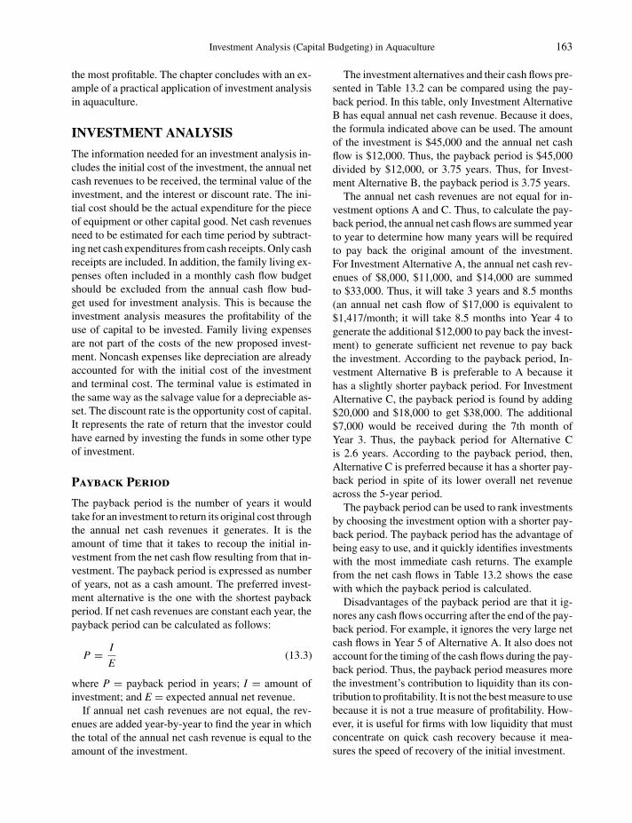
P1: SFK/UKS P2: SFK



the most profitable. The chapter concludes with an ex-ample of a practical application of investment analysisin aquaculture.

INVESTMENT ANALYSIS

The information needed for an investment analysis in-cludes the initial cost of the investment, the annual netcash revenues to be received, the terminal value of theinvestment, and the interest or discount rate. The ini-tial cost should be the actual expenditure for the pieceof equipment or other capital good. Net cash revenuesneed to be estimated for each time period by subtract-ing net cash expenditures from cash receipts. Only cashreceipts are included. In addition, the family living ex-penses often included in a monthly cash flow budgetshould be excluded from the annual cash flow bud-get used for investment analysis. This is because theinvestment analysis measures the profitability of theuse of capital to be invested. Family living expensesare not part of the costs of the new proposed invest-ment. Noncash expenses like depreciation are alreadyaccounted for with the initial cost of the investmentand terminal cost. The terminal value is estimated inthe same way as the salvage value for a depreciable as-set. The discount rate is the opportunity cost of capital.It represents the rate of return that the investor couldhave earned by investing the funds in some other typeof investment.

Payback Period

The payback period is the number of years it wouldtake for an investment to return its original cost throughthe annual net cash revenues it generates. It is theamount of time that it takes to recoup the initial in-vestment from the net cash flow resulting from that in-vestment. The payback period is expressed as numberof years, not as a cash amount. The preferred invest-ment alternative is the one with the shortest paybackperiod. If net cash revenues are constant each year, thepayback period can be calculated as follows:

P = I

E(13.3)

where P = payback period in years; I = amount ofinvestment; and E = expected annual net revenue.

If annual net cash revenues are not equal, the rev-enues are added year-by-year to find the year in whichthe total of the annual net cash revenue is equal to theamount of the investment.

The investment alternatives and their cash flows pre-sented in Table 13.2 can be compared using the pay-back period. In this table, only Investment AlternativeB has equal annual net cash revenue. Because it does,the formula indicated above can be used. The amountof the investment is $45,000 and the annual net cashflow is $12,000. Thus, the payback period is $45,000divided by $12,000, or 3.75 years. Thus, for Invest-ment Alternative B, the payback period is 3.75 years.

The annual net cash revenues are not equal for in-vestment options A and C. Thus, to calculate the pay-back period, the annual net cash flows are summed yearto year to determine how many years will be requiredto pay back the original amount of the investment.For Investment Alternative A, the annual net cash rev-enues of $8,000, $11,000, and $14,000 are summedto $33,000. Thus, it will take 3 years and 8.5 months(an annual net cash flow of $17,000 is equivalent to$1,417/month; it will take 8.5 months into Year 4 togenerate the additional $12,000 to pay back the invest-ment) to generate sufficient net revenue to pay backthe investment. According to the payback period, In-vestment Alternative B is preferable to A because ithas a slightly shorter payback period. For InvestmentAlternative C, the payback period is found by adding$20,000 and $18,000 to get $38,000. The additional$7,000 would be received during the 7th month ofYear 3. Thus, the payback period for Alternative Cis 2.6 years. According to the payback period, then,Alternative C is preferred because it has a shorter pay-back period in spite of its lower overall net revenueacross the 5-year period.

The payback period can be used to rank investmentsby choosing the investment option with a shorter pay-back period. The payback period has the advantage ofbeing easy to use, and it quickly identifies investmentswith the most immediate cash returns. The examplefrom the net cash flows in Table 13.2 shows the easewith which the payback period is calculated.

Disadvantages of the payback period are that it ig-nores any cash flows occurring after the end of the pay-back period. For example, it ignores the very large netcash flows in Year 5 of Alternative A. It also does notaccount for the timing of the cash flows during the pay-back period. Thus, the payback period measures morethe investment’s contribution to liquidity than its con-tribution to profitability. It is not the best measure to usebecause it is not a true measure of profitability. How-ever, it is useful for firms with low liquidity that mustconcentrate on quick cash recovery because it mea-sures the speed of recovery of the initial investment.

P1: SFK/UKS P2: SFK



Simple Rate of Return

The simple rate of return expresses average annual netrevenue as a percentage of the investment. Net revenueis found by subtracting the average annual depreciationfrom the average annual net cash revenue.

The formula used is:

Average annual net revenue

Cost of the investment× 100 (13.4)

For the three investment options in Table 13.2, then,the simple rate of return is:

Investment A $14,000 divided by $45,000, or 31%Investment B $12,000 divided by $45,000, or 27%Investment C $12,600 divided by $45,000, or 28%.

Thus, according to the simple rate of return, the prefer-able option is A, with the highest rate of return, fol-lowed by C and then B. Alternatives B and C earn asimilar rate of return because the average annual netcash flow is similar. This method does not account forthe substantial difference in the pattern of cash flow.

The simple rate of return is an improvement overthe payback period in terms of measuring profitabilitybecause it considers the earnings of an investment overthe entire life of the investment. However, there is amajor disadvantage in that it fails to consider the sizeand timing of the annual earnings and can thereforecause errors in selecting investments. This is especiallytrue when net revenues are increasing or decreasing.

Net Present Value

NPV is also known as the discounted cash flowmethod. NPV is equal to the sum of the PVs for eachyear’s net cash flow less the initial cost of the invest-ment. PV is equal to the current value of a sum ofmoney to be received or paid in the future. It is foundwith discounting and is equal to the sum of PVs foreach year’s net cash flow less the initial cost of the in-vestment. It can also be viewed as that sum of moneywhich would have to be invested now at the given inter-est rate to equal the FV on the same date. Figure 13.1illustrates the stream of net cash flow for InvestmentAlternative B.

Mathematically, NPV is calculated as follows:

NPV = P1

(1 + I )1+ P2

(1 + I )2

+ · · · Pn

(1 + I )n− C (13.5)

where NPV = net present value; Pn = net cash flowin year, n; I = discount rate; and c = initial cost ofinvestment.

Investments with a positive NPV would be accepted;those with a negative NPV rejected, and a zero valuemakes the investor indifferent. With a positive NPV,the rate of return of the investment is higher than thediscount rate used, and it is greater than the opportunitycost of capital used as the discount rate. Projects witha greater NPV are the most favored. The limitations ofthe NPV analysis are that it depends on the discountrate and that it does not determine the actual rate ofreturn.

NPV can be calculated with a hand calculator orspreadsheet based software, such as Microsoft R© Ex-cel. The NPV for the three investment alternatives pre-sented in Table 13.2 were calculated using an Excelspreadsheet with the NPV function. When the NPVfunction is selected, a dialogue box opens that asksfor the discount rate. If the prevailing cost of capital(interest rate) is 10%, for example, then the discountrate is expressed as 0.10. Once the discount rate isentered, the NPV function dialogue box then asks forthe values. The first value in the row should be thetotal investment amount, expressed as a negative num-ber (Figure 13.1). The second value is the net cashflow for Year 1, followed by the net cash flow forYear 2.

The NPV that is calculated is expressed as a dollarvalue. If it is positive, then the investment is profitablebecause the flow of returns, after accounting for thetime value of money at the discount rate (interest rate)selected, is above 0. If the NPV is negative, then the in-vestment earns less than its opportunity cost (discountrate or interest rate that would have been earned by theinvestment) and is not profitable.

For the three investment options listed in Table 13.2,Alternative C has the highest NPV ($5,987), followedby Alternative A ($5,374), and then Alternative B($445) (Table 13.3). Strictly speaking, NPV values,technically, should not be compared to rank invest-ments. Each of these options has a positive NPV and,thus, all are profitable investments.

The limitation of the NPV is that the value calculateddepends upon the discount rate selected. Varying dis-count rates will change the NPV. Moreover, the NPVdoes not calculate the rate of return actually earnedby the investment. The other drawback of the NPV isthat the size of the NPV is affected by the size of theinvestment. To overcome this limitation, a profitabilityindex can be calculated by dividing the total PV of the

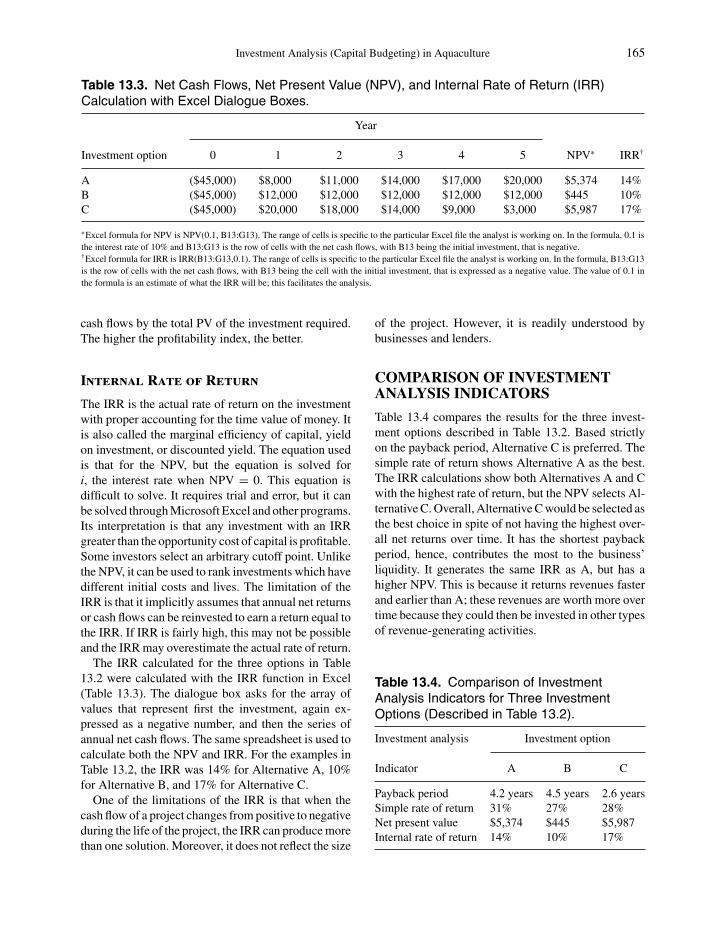
P1: SFK/UKS P2: SFK



Table 13.3. Net Cash Flows, Net Present Value (NPV), and Internal Rate of Return (IRR)Calculation with Excel Dialogue Boxes.

Year

Investment option 0 1 2 3 4 5 NPV∗ IRR†

A ($45,000) $8,000 $11,000 $14,000 $17,000 $20,000 $5,374 14%B ($45,000) $12,000 $12,000 $12,000 $12,000 $12,000 $445 10%C ($45,000) $20,000 $18,000 $14,000 $9,000 $3,000 $5,987 17%

∗Excel formula for NPV is NPV(0.1, B13:G13). The range of cells is specific to the particular Excel file the analyst is working on. In the formula, 0.1 isthe interest rate of 10% and B13:G13 is the row of cells with the net cash flows, with B13 being the initial investment, that is negative.†Excel formula for IRR is IRR(B13:G13,0.1). The range of cells is specific to the particular Excel file the analyst is working on. In the formula, B13:G13is the row of cells with the net cash flows, with B13 being the cell with the initial investment, that is expressed as a negative value. The value of 0.1 inthe formula is an estimate of what the IRR will be; this facilitates the analysis.

cash flows by the total PV of the investment required.The higher the profitability index, the better.

Internal Rate of Return

The IRR is the actual rate of return on the investmentwith proper accounting for the time value of money. Itis also called the marginal efficiency of capital, yieldon investment, or discounted yield. The equation usedis that for the NPV, but the equation is solved fori, the interest rate when NPV = 0. This equation isdifficult to solve. It requires trial and error, but it canbe solved through Microsoft Excel and other programs.Its interpretation is that any investment with an IRRgreater than the opportunity cost of capital is profitable.Some investors select an arbitrary cutoff point. Unlikethe NPV, it can be used to rank investments which havedifferent initial costs and lives. The limitation of theIRR is that it implicitly assumes that annual net returnsor cash flows can be reinvested to earn a return equal tothe IRR. If IRR is fairly high, this may not be possibleand the IRR may overestimate the actual rate of return.

The IRR calculated for the three options in Table13.2 were calculated with the IRR function in Excel(Table 13.3). The dialogue box asks for the array ofvalues that represent first the investment, again ex-pressed as a negative number, and then the series ofannual net cash flows. The same spreadsheet is used tocalculate both the NPV and IRR. For the examples inTable 13.2, the IRR was 14% for Alternative A, 10%for Alternative B, and 17% for Alternative C.

One of the limitations of the IRR is that when thecash flow of a project changes from positive to negativeduring the life of the project, the IRR can produce morethan one solution. Moreover, it does not reflect the size

of the project. However, it is readily understood bybusinesses and lenders.

COMPARISON OF INVESTMENTANALYSIS INDICATORS

Table 13.4 compares the results for the three invest-ment options described in Table 13.2. Based strictlyon the payback period, Alternative C is preferred. Thesimple rate of return shows Alternative A as the best.The IRR calculations show both Alternatives A and Cwith the highest rate of return, but the NPV selects Al-ternative C. Overall, Alternative C would be selected asthe best choice in spite of not having the highest over-all net returns over time. It has the shortest paybackperiod, hence, contributes the most to the business’liquidity. It generates the same IRR as A, but has ahigher NPV. This is because it returns revenues fasterand earlier than A; these revenues are worth more overtime because they could then be invested in other typesof revenue-generating activities.

Table 13.4. Comparison of InvestmentAnalysis Indicators for Three InvestmentOptions (Described in Table 13.2).

Investment analysis Investment option

Indicator A B C

Payback period 4.2 years 4.5 years 2.6 yearsSimple rate of return 31% 27% 28%Net present value $5,374 $445 $5,987Internal rate of return 14% 10% 17%

P1: SFK/UKS P2: SFK



RELATIONSHIP BETWEEN NPVAND IRR

NPV and IRR are closely related. This is because theyboth are based on net cash flows that use the same dis-counting method. The difference is that the calculationof NPV requires that a discount (interest) rate be spec-ified at the outset. IRR, on the other hand, computesthe interest rate that yields a zero NPV. The IRR andNPV typically result in the same rankings of projects,although there are some exceptions.

DATA REQUIREMENTS FORINVESTMENT ANALYSIS(CAPITAL BUDGETING)

The amount of the initial investment must first be deter-mined. This is the amount of funds that the investor orowner is willing to commit to the project or investment.The total amount of investment must include all costsassociated with the investment. These include anytaxes, transportation charges, installation costs associ-ated with roads, or electrical supply in addition to thepurchase cost of the asset. If there is a trade-in value,it should be subtracted from the purchase amount.

Net cash flows measure the expected future returnsfor the investment alternatives. Net cash flows are ob-tained by subtracting out cash outflows from cash re-ceipts for each time period. Net cash flows are notprofits because noncash items are not included. At theend of the planning horizon (10 years for a 10-year cashflow budget), whatever remaining value exists in cap-ital goods is included as a terminal or residual value.

The planning horizon for the analysis must be spec-ified. One factor that is important in deciding on thelength of the planning horizon is the useful life of theasset. If the analysis were for an investment in a newpiece of equipment, an appropriate planning horizonwould be the useful life of the capital good.

RECORD-KEEPING

Investment analysis combines records maintained forother purposes on the farm. Essentially, enterprisebudget-style cost analyses must be developed. Thetypes of information and records required for a properenterprise budget can be found in Chapter 10.

Once an investment analysis has been developed,the Excel files associated with it should be maintained.These can be used as templates for future analyses orto develop sensitivity analyses related to variations inparameter values to evaluate other conditions.

PRACTICAL APPLICATION:DOUBLING THE NUMBER OFAERATORS ON A 256-ACRECATFISH FARM

An example of an investment decision on a fish farmwould be the decision to expand aeration capacity from1 hp/acre to 2 hp/acre. For a 10-acre pond, then, thiswould require adding 1 additional 10-hp aerator toeach pond to supplement the existing 10-hp aerator.For the 256-acre farm that has 25 10-acre ponds, anadditional 25 aerators would need to be purchased. Ata cost of $4,500, the additional investment would be$112,500 for the farm.

The benefit of expanding aeration capacity wouldbe the ability to maintain higher levels of dissolvedoxygen in the pond. Higher levels of oxygen would beexpected to result in higher yields (lb/acre) of catfish.Thus, if yield increased by 500 lb/acre and catfish pricewas $0.70/lb, the additional revenue would be $89,600.The additional weight of fish sold would require ad-ditional harvesting and seining costs. Electricity costswould also increase. The total increase in use of elec-tricity was assumed to be 90%, instead of a doublingof use, because aerators would be turned on sequen-tially as oxygen begins to fall. This example analysisassumed that a 5-year loan was taken out at a 10%interest rate, to finance the purchase of the aerators.

Table 13.5 shows the results of the investment anal-ysis. The payback period would be 3.3 years with aNPV of $16,038 (10% discount rate) and an IRR of16%. Thus, under the assumptions used in this analy-sis, the expansion of aeration capacity is a profitableinvestment. Additional yields above 500 lb/acre, cat-fish prices above $0.70/lb, electricity usage less thanthat assumed, or lower electric rates would result ingreater profit levels. Conversely, if yield remained thesame, this investment would not be profitable. If ad-ditional yields were less than 500 lb/acre, or if catfishprices were lower or more electricity would be used,the profitability of this investment would be reduced.


Trimpey and Engle (2005) used an investment analysisto evaluate the profitability of purchasing an in-pondmechanical grader for food-sized channel catfish. Thecost of a commercial-scale version of the grader wasestimated. Benefits were estimated on the basis of tri-als of the efficiency of the grader in both experimental

P1: SFK/UKS P2: SFK



Table 13.5. Annual Cash Flow Budget for Investment Analysis of Adding 1 hp/acre of AdditionalAeration to a 256-acre Farm.

Item Year 0 Year 1 Year 2 Year 3 Year 4 Year 5

Cash receipts 89,600 89,600 89,600 89,600 89,600Cash inflow 89,600 89,600 89,600 89,600 89,600Operating expenses

Fingerlings — — — — —Feed — — — — —Fertilizer — — — — —Chemicals — — — — —Labor — — — — —Electricity 44,390 44,390 44,390 44,390 44,390Diesel — — — — —Gasoline — — — — —Repairs and maintenance — — — — —Levee repairs — — — — —Postharvest handling 6,400 6,400 6,400 6,400 6,400Marketing — — — — —Insurance — — — — —

Total 50,790 50,790 50,790 50,790 50,790Capital expenditures — — — — —Other expenses — — — — —Scheduled debt payments

Principal—real estate — — — — —Interest — — — — —Principal—equipment 22,500 22,500 22,500 22,500 22,500Interest 4,479 4,479 4,479 4,479 4,479Principal—operating — — — — —Interest — — — — —

Total cash outflow 55,269 55,269 55,269 55,269 55,269Cash available 34,331 34,331 34,331 34,331 34,331New borrowing — — — — —Cash balance 34,331 34,331 34,331 34,331 34,331Debt outstanding

Real estate — — — — —Equipment 90,000 67,500 45,000 22,500 —Operating — — — — —

Net cash flow (112,500) 34,331 34,331 34,331 34,331 34,331Net present value (NPV) Discount rate 0.10

NPV 16,038Internal rate of return (IRR) IRR 16%

and commercial catfish ponds. The trials provided dataon the size distributions of fish harvested from the tra-ditional live car passive grading system and the activemechanical grader. Various scenarios of deductionsfrom processing plants for out-of-size fish were usedto compare the relative benefits for the size distribu-tions of fish from the traditional, passive technologyto the active mechanical technology.

The results showed payback periods from 0.1 to 2.0years. The mechanical grader was shown to be prof-itable with positive NPVs and internal rates of returnthat were greater than the current opportunity cost ofcapital. Both NPV and internal rates of return increasedwith farm size. The analysis showed that it was eco-nomically feasible to adopt the in-pond mechanicalgrader.

P1: SFK/UKS P2: SFK


Tab

le13

.6.

Fut

ure

Val

ueof

a$1

Inve

stm

ent.

Yea

rs4%

4.5%

5%5.

5%6%

6.5%

7%7.

5%8%

8.5%

9%9.

5%10

%

11.

0400

1.04

501.

0500

1.05

501.

0600

1.06

501.

0700

1.07

501.

0800

1.08

501.

0900

1.09

501.

1000

21.

0816

1.09

201.

1025

1.11

301.

1236

1.13

421.

1449

1.15

561.

1664

1.17

721.

1881

1.19

901.

2100

31.

1249

1.14

121.

1576

1.17

421.

1910

1.20

791.

2250

1.24

231.

2597

1.27

731.

2950

1.31

291.

3310

41.

1699

1.19

251.

2155

1.23

881.

2625

1.28

651.

3108

1.33

551.

3605

1.38

591.

4116

1.43

771.

4641

51.

2167

1.24

621.

2763

1.30

701.

3382

1.37

011.

4026

1.43

561.

4693

1.50

371.

5386

1.57

421.

6105

61.

2653

1.30

231.

3401

1.37

881.

4185

1.45

911.

5007

1.54

331.

5869

1.63

151.

6771

1.72

381.

7716

71.

3159

1.36

091.

4071

1.45

471.

5036

1.55

401.

6058

1.65

901.

7138

1.77

011.

8280

1.88

761.

9487

81.

3686

1.42

211.

4775

1.53

471.

5938

1.65

501.

7182

1.78

351.

8509

1.92

061.

9926

2.06

692.

1436

91.

4233

1.48

611.

5513

1.61

911.

6895

1.76

261.

8385

1.91

721.

9990

2.08

392.

1719

2.26

322.

3579

101.

4802

1.55

301.

6289

1.70

811.

7908

1.87

711.

9672

2.06

102.

1589

2.26

102.

3674

2.47

822.

5937

111.

5395

1.62

291.

7103

1.80

211.

8983

1.99

922.

1049

2.21

562.

3316

2.45

322.

5804

2.71

372.

8531

121.

6010

1.69

591.

7959

1.90

122.

0122

2.12

912.

2522

2.38

182.

5182

2.66

172.

8127

2.97

153.

1384

131.

6651

1.77

221.

8856

2.00

582.

1329

2.26

752.

4098

2.56

042.

7196

2.88

793.

0658

3.25

373.

4523

141.

7317

1.85

191.

9799

2.11

612.

2609

2.41

492.

5785

2.75

242.

9372

3.13

343.

3417

3.56

293.

7975

151.

8009

1.93

532.

0789

2.23

252.

3966

2.57

182.

7590

2.95

893.

1722

3.39

973.

6425

3.90

134.

1772

161.

8730

2.02

242.

1829

2.35

532.

5404

2.73

902.

9522

3.18

083.

4259

3.68

873.

9703

4.27

194.

5950

171.

9479

2.11

342.

2920

2.48

482.

6928

2.91

703.

1588

3.41

943.

7000

4.00

234.

3276

4.67

785.

0545

182.

0258

2.20

852.

4066

2.62

152.

8543

3.10

673.

3799

3.67

583.

9960

4.34

254.

7171

5.12

225.

5599

192.

1068

2.30

792.

5270

2.76

563.

0256

3.30

863.

6165

3.95

154.

3157

4.71

165.

1417

5.60

886.

1159

202.

1911

2.41

172.

6533

2.91

783.

2071

3.52

363.

8697

4.24

794.

6610

5.11

205.

6044

6.14

166.

7275

212.

2788

2.52

022.

7860

3.07

823.

3996

3.75

274.

1406

4.56

645.

0338

5.54

666.

1088

6.72

517.

4002

222.

3699

2.63

372.

9253

3.24

753.

6035

3.99

664.

4304

4.90

895.

4365

6.01

806.

6586

7.36

398.

1403

232.

4647

2.75

223.

0715

3.42

623.

8197

4.25

644.

7405

5.27

715.

8715

6.52

967.

2579

8.06

358.

9543

242.

5633

2.87

603.

2251

3.61

464.

0489

4.53

315.

0724

5.67

296.

3412

7084

67.

9111

8.82

969.

8497

252.

6658

3.00

543.

3864

3.81

344.

2919

4.82

775.

4274

6.09

836.

8485

7.68

688.

6231

9.66

8410

.834

730

3.24

343.

7453

4.32

194.

9840

5.74

356.

6144

7.61

238.

7550

10.0

627

11.5

583

13.2

677

15.2

203

17.4

494

353.

9461

4.66

735.

5160

6.51

387.

6861

9.06

2310

.676

612

.568

8914

.785

317

.379

620

.414

023

.960

428

.102

440

4.80

105.

8164

7.04

008.

5133

10.2

857

12.4

161

14.9

475

18.0

442

21.7

245

26.1

330

31.4

094

37.7

194

45.2

593

P1: SFK/UKS P2: SFK


Yea

rs10

.5%

11%

11.5

%12

%12

.5%

13%

13.5

%14

%14

.5%

15%

15.5

%16

%16

.5%

11.

1050

1.11

001.

1150

1.12

001.

1250

1.13

001.

1350

1.14

001.

1450

1.15

001.

1550

1.16

001.

1650

21.

2210

1.23

211.

2432

1.25

441.

2656

1.27

691.

2882

1.29

961.

3110

1.32

251.

3340

1.34

561.

3572

31.

3492

1.36

761.

3862

1.40

491.

4238

1.44

291.

4621

1.48

151.

5011

1.52

091.

5408

1.56

091.

5812

41.

4909

1.51

811.

5456

1.57

351.

6018

1.63

051.

6595

1.68

901.

7188

1.74

901.

7796

1.81

061.

8421

51.

6474

1.68

511.

7234

1.76

231.

8020

1.84

241.

8836

1.92

541.

9680

2.01

142.

0555

2.10

032.

1460

61.

8204

1.87

041.

9215

1.97

382.

0273

2.08

202.

1378

2.19

502.

2534

2.31

312.

3741

2.43

642.

5001

72.

0116

2.07

622.

1425

2.21

072.

2807

2.35

262.

4264

2.50

232.

5801

2.66

002.

7420

2.82

622.

9126

82.

2228

2.30

452.

3889

2.47

602.

5658

2.65

842.

7540

2.85

262.

9542

3.05

903.

1671

3.27

843.

3932

92.

4562

2.55

802.

6636

2.77

312.

8865

3.00

403.

1258

3.25

193.

3826

3.51

793.

6580

3.80

303.

9531

102.

7141

2.83

942.

9699

3.10

583.

2473

3.39

463.

5478

3.70

723.

8731

4.04

564.

2249

4.41

144.

6053

112.

9991

3.15

183.

3115

3.47

853.

6532

3.83

594.

0267

4.22

624.

4347

4.65

244.

8798

5.11

735.

3652

123.

3140

3.49

853.

6923

3.89

604.

1099

4.33

454.

5704

4.81

795.

0777

5.35

035.

6362

5.93

606.

2504

133.

6619

3.88

334.

1169

4.36

354.

6236

4.89

805.

1874

5.49

245.

8140

6.15

286.

5098

6.88

587.

2818

144.

0464

4310

44.

5904

4.88

715.

2016

5.53

485.

8877

6.26

136.

6570

7.07

577.

5188

7.98

758.

4833

154.

4713

4.78

465.

1183

5.47

365.

8518

6.25

436.

6825

7.13

797.

6222

8.13

718.

6842

9.26

559.

8830

164.

9408

5.31

095.

7069

6.13

046.

5833

7.06

737.

5846

8.13

728.

7275

9.35

7610

.030

210

.748

011

.513

717

5.45

965.

8951

6.36

326.

8660

7.40

627.

9861

8.60

859.

2765

9.99

2910

.761

311

.584

912

.467

713

.413

518

6.03

286.

5436

7.09

497.

6900

8.33

199.

0243

9.77

0710

.575

211

.441

912

.375

513

.380

614

.462

515

.626

719

6.66

637.

2633

7.91

088.

6128

9.37

3410

.197

411

.089

712

.055

713

.101

014

.231

815

.454

616

.776

518

.205

120

7.36

628.

0623

8.82

069.

6463

10.5

451

11.5

231

12.5

869

13.7

435

15.0

006

16.3

665

17.8

501

19.4

608

21.2

089

218.

1397

8.94

929.

8350

10.8

038

11.8

632

13.0

211

14.2

861

15.6

676

17.1

757

18.8

215

20.6

168

22.5

745

24.7

084

228.

9944

9.93

3610

.966

012

.100

313

.346

114

.713

816

.214

717

.861

019

.666

221

.644

723

.812

426

.186

428

.785

323

9.93

8811

.026

312

.227

113

.552

315

.014

416

.626

618

.403

720

.361

622

.517

824

.891

527

.503

430

.376

233

.534

824

10.9

823

12.2

392

13.6

332

15.1

786

16.8

912

18.7

881

20.8

882

23.2

122

25.7

829

28.6

252

31.7

664

35.2

364

39.0

681

2512

.135

513

.585

515

.201

017

.000

119

.002

621

.230

523

.708

126

.461

929

.521

432

.919

036

.690

240

.874

245

.514

330

19.9

926

22.8

923

26.1

967

29.9

599

34.2

433

39.1

159

44.6

556

50.9

502

58.0

985

66.2

118

75.4

153

85.8

499

97.6

737

3532

.936

738

.574

945

.146

152

.799

661

.707

572

.068

584

.111

598

.100

211

4.33

8413

3.17

5515

5.01

3518

0.31

4120

9.60

7840

54.2

614

65.0

009

77.8

027

93.0

510

111.

1990

132.

7816

158.

4289

188.

8835

225.

0191

267.

8635

318.

6246

378.

7212

449.

8182

P1: SFK/UKS P2: SFK


Tab

le13

.7.

Pre

sent

Val

ueof

a$1

Lum

pS

um.

Yea

rs4%

4.5%

5%5.

5%6%

6.5%

7%7.

5%8%

8.5%

9%9.

5%10

%

10.

9615

40.

9569

40.

9523

80.

9478

70.

9434

00.

9389

70.

9345

80.

9302

30.

9259

30.

9216

60.

9174

30.

9132

40.

9090

92

0.92

456

0.91

573

0.90

703

0.89

845

0.89

000

0.88

166

0.87

344

03.8

6533

0.85

734

0.84

946

0.84

168

0.83

401

0.82

645

30.

8890

00.

8763

00.

8638

40.

8516

10.

8396

20.

8278

50.

8163

00.

8049

60.

7938

30.

7829

10.

7721

80.

7616

50.

7513

14

0.85

480

0.83

856

0.82

270

0.80

722

0.79

209

0.77

732

0.76

290

0.74

880

0.73

503

0.72

157

0.70

843

0.69

557

0.68

301

50.

8219

30.

8024

50.

7835

30.

7651

30.

7472

60.

7298

80.

7129

90.

6965

60.

6805

80.

6650

50.

6499

30.

6352

30.

6209

26

0.79

031

0.76

790

0.74

622

0.72

525

0.70

496

0.68

533

0.66

634

0.64

796

0.63

017

0.61

295

0.59

627

0.58

012

0.56

447

70.

7599

20.

7348

30.

7106

80.

6874

40.

6650

60.

6435

10.

6227

50.

6027

50.

5834

90.

5649

30.

5470

30.

5297

90.

5131

68

0.73

069

0.70

319

0.67

684

0.65

160

0.62

741

0.60

423

0.58

201

0.56

070

0.54

027

0.52

067

0.50

187

0.48

382

0.46

651

90.

7025

90.

6729

00.

6446

10.

6176

30.

5919

00.

5673

50.

5439

30.

5215

80.

5002

50.

4798

80.

4604

30.

4418

50.

4241

010

0.67

556

0.64

393

0.61

391

0.58

543

0.55

839

0.53

273

0.50

835

0.48

519

0.46

319

0.44

229

0.42

214

0.40

351

0.38

554

110.

6495

80.

6162

005

8468

0.55

491

0.52

679

0.50

021

0.47

509

0.45

134

0.42

888

0.40

764

0.38

753

0.36

851

0.35

049

120.

6246

00.

5896

60.

5568

40.

5259

80.

4969

70.

4696

80.

4440

10.

4198

50.

3971

10.

3757

00.

3555

30.

3365

40.

3186

313

0.60

057

0.56

427

0.53

032

0.49

856

0.46

884

0.44

102

0.41

496

0.39

056

0.36

770

0.34

627

0.32

618

0.30

734

0.28

966

140.

5774

80.

5399

70.

5050

70.

4725

70.

4423

00.

4141

00.

3878

20.

3633

10.

3404

60.

3191

40.

2992

50.

2806

70.

2633

315

0.55

526

0.51

672

0.48

102

0.44

793

0.41

727

0.38

883

0.36

245

0.33

797

0.31

524

0.29

414

0.27

454

0.25

632

0.23

939

160.

5339

10.

4944

70.

4581

10.

4245

80.

3936

50.

3651

00.

3387

30.

3143

90.

2918

90.

2711

00.

2518

70.

2340

90.

2176

317

0.51

337

0.47

318

0.43

630

0.40

245

0.37

136

0.34

281

0.31

657

0.29

245

0.27

027

0.24

986

0.23

107

0.21

378

0.19

784

180.

4936

30.

4528

00.

4155

20.

3814

70.

3503

40.

3218

90.

2958

60.

2720

50.

2502

50.

2302

80.

2119

90.

1952

30.

1798

619

0.47

464

0.43

330

0.39

573

0.36

158

0.33

051

0.30

224

0.27

651

0.25

307

0.23

171

0.21

224

0.19

449

0.17

829

0.16

351

200.

4563

90.

4146

40.

3768

90.

3427

30.

3118

00.

2838

00.

2584

20.

2354

10.

2145

50.

1956

20.

1784

30.

1628

20.

1486

421

0.43

883

0.39

679

0.35

894

0.32

486

0.29

416

0.26

648

0.24

151

0.21

899

0.19

866

0.18

029

0.16

370

0.14

870

0.13

513

220.

4219

60.

3797

00.

3418

50.

3079

30.

2775

10.

2502

10.

2257

10.

2037

10.

1839

40.

1661

70.

1501

80.

1358

00.

1228

523

0.40

573

0.36

335

0.32

557

0.29

187

0.26

180

0.23

494

0.21

095

0.18

950

0.17

032

0.15

315

0.13

778

0.12

402

0.11

168

240.

3901

20.

3477

00.

3100

70.

2766

60.

2469

80.

2206

00.

1971

50.

1762

80.

1577

00.

1411

50.

1264

00.

1132

60.

1015

325

0.37

512

0.33

273

0.29

530

0.26

223

0.23

300

0.20

714

0.18

425

0.16

398

0.14

602

0.13

009

0.11

597

0.10

343

0.09

230

300.

3083

20.

2670

00.

2313

80.

2006

40.

1741

10.

1511

90.

1313

70.

1142

20.

0993

80.

0865

20.

0753

70.

0657

00.

0573

135

0.25

342

0.21

425

0.18

129

0.15

352

0.13

011

0.11

035

0.09

366

0.07

956

0.06

763

0.05

754

0.04

899

0.04

174

0.03

558

400.

2082

90.

1719

30.

1420

0.11

746

0.09

722

0.08

054

0.06

678

0.05

542

0.04

603

0.03

827

0.03

184

0.02

651

0.02

209

P1: SFK/UKS P2: SFK


Yea

rs10

.5%

11%

11.5

%12

%12

.5%

13%

13.5

%14

%14

.5%

15%

15.5

%16

%16

.5%

10.

9049

80.

9009

00.

8968

60.

8928

60.

8888

90.

8849

60.

8810

60.

8771

90.

8733

60.

8695

70.

8658

00.

8620

70.

8583

72

0.81

898

0.81

162

0.80

436

0.79

719

0.79

012

0.78

315

0.77

626

0.76

947

0.76

276

0.75

614

0.74

961

0.74

316

0.73

680

30.

7411

60.

7311

90.

7214

00.

7117

80.

7023

30.

6930

50.

6839

30.

6749

70.

6661

70.

6575

20.

6490

10.

6406

60.

6324

44

0.67

073

0.65

873

0.64

699

0.63

552

0.62

430

0.61

332

0.60

258

0.59

208

0.58

181

0.57

175

0.56

192

0.55

229

0.54

287

50.

6070

00.

5934

50.

5802

60.

5674

30.

5549

30.

5427

60.

5309

10.

5193

70.

5081

30.

4971

80.

4865

10.

4761

10.

4659

86

0.54

932

0.53

464

0.52

042

0.50

663

0.49

327

0.48

032

0.46

776

0.45

559

0.44

378

0.43

233

0.42

122

0.41

044

0.39

999

70.

4971

20.

4816

60.

4667

40.

4523

50.

4384

60.

4250

60.

4121

30.

3996

40.

3875

80.

3759

40.

3646

90.

3538

30.

3433

48

0.44

989

0.43

393

0.41

860

0.40

388

0.38

974

0.37

616

0.36

311

0.35

056

0.33

850

0.32

690

0.31

575

0.30

503

0.29

471

90.

4071

40.

3909

20.

3754

30.

3606

10.

3464

40.

3328

80.

3199

20.

3075

10.

2956

30.

2842

60.

2733

80.

2629

50.

2529

710

0.36

845

0.35

218

0.33

671

0.32

197

0.30

795

0.29

459

0.28

187

0.26

974

0.25

819

0.24

718

0.23

669

0.22

668

0.21

714

110.

3334

40.

3172

80.

3019

80.

2874

80.

2737

30.

2607

00.

2483

40.

2366

20.

2255

00.

2149

40.

2049

30.

1954

20.

1863

912

0.30

175

0.28

584

0.27

083

0.25

668

0.24

332

0.23

071

0.21

880

0.20

756

0.19

694

0.18

691

0.17

743

0.16

846

0.15

999

130.

2730

80.

2575

10.

2429

00.

2291

70.

2162

80.

2041

60.

1927

80.

1820

70.

1720

00.

1625

30.

1536

20.

1452

30.

1373

314

0.24

713

0.23

199

0.21

785

0.20

462

0.19

225

0.18

068

0.16

985

0.15

971

0.15

022

0.14

133

0.13

300

0.12

520

0.11

788

150.

2236

50.

2090

00.

1953

80.

1827

00.

1708

90.

1598

90.

1496

40.

1401

00.

1312

00.

1228

90.

1151

50.

1079

30.

1011

816

0.20

240

0.18

829

0.17

523

0.16

312

0.15

190

0.14

150

0.13

185

0.12

289

0.11

458

0.10

686

0.09

970

0.09

304

0.08

685

170.

1831

60.

1696

30.

1571

50.

1456

40.

1350

20.

1252

20.

1161

60.

1078

00.

1000

70.

0929

30.

0863

20.

0802

10.

0745

518

0.16

576

0.15

282

0.14

095

0.13

004

0.12

002

0.11

081

0.10

235

0.09

456

0.08

740

0.08

081

0.07

474

0.06

914

0.06

399

190.

1500

10.

1376

80.

1264

10.

1161

10.

1066

80.

0980

60.

0901

70.

0829

50.

0763

30.

0702

70.

0647

10.

0596

10.

0549

320

0.13

575

0.12

403

0.11

337

0.10

367

0.09

483

0.08

678

0.07

945

0.07

276

0.06

666

0.06

110

0.05

602

0.05

139

0.04

715

210.

1228

50.

1117

40.

1016

80.

0925

60.

0842

90.

0768

00.

0700

00.

0638

30.

0582

20.

0531

30.

0485

00.

0443

00.

0404

722

0.11

118

0.10

067

0.09

119

0.08

264

0.07

493

0.06

796

0.06

167

0.05

599

0.05

085

0.04

620

0.04

199

0.03

819

0.03

474

230.

1006

20.

0906

90.

0817

90.

0737

90.

0666

00.

0601

40.

0543

40.

0491

10.

0444

10.

0401

70.

0363

60.

0329

20.

0298

224

0.09

106

0.08

170

0.07

335

0.06

588

0.05

920

0.05

323

0.04

787

0.04

308

0.03

879

0.03

493

0.03

148

0.02

838

0.02

560

250.

0824

00.

0736

10.

0657

90.

0588

20.

0526

20.

0471

00.

0421

80.

0377

90.

0338

70.

0303

80.

0272

60.

0244

70.

0219

730

0.05

002

0.04

368

0.03

817

0.03

338

0.02

920

0.02

557

0.02

239

0.01

963

0.01

721

0.01

510

0.01

326

0.01

165

0.01

024

350.

0303

60.

0259

20.

0221

50.

0159

40.

0162

10.

0138

80.

0118

90.

0101

90.

0087

50.

0075

10.

0064

50.

0055

50.

0044

7740

0.01

843

0.01

538

0.01

285

0.01

075

0.00

899

0.00

753

0.00

631

0.00

529

0.00

444

0.00

373

0.00

314

0.00

264

0.00

222

P1: SFK/UKS P2: SFK



SUMMARY

Investments in assets that will be used over a period ofyears must be evaluated differently from operating in-puts because of the time periods involved. Many aqua-culture businesses are capital-intensive and require agreat deal of capital investment. Thus, understandinghow to evaluate and manage these investments from afinancial perspective is important.

The time value of money is central to understandinghow to analyze these investments. Investment capitalhas an initial PV that can be invested at a particularinterest rate to compound over time into a FV. Con-versely, the returns generated over a period of yearsin the future (FV) can be discounted back to calculatetheir PV.

The most commonly used types of investment anal-yses are the payback period, NPV, and the internal rateor return. The payback period is simple to calculateand provides a measure of the contribution to liquidityof an investment by indicating how many years it willtake to recover the amount of the investment. However,the payback period does not consider revenue gener-ated beyond that point in time and does not account forthe timing of cash flows. The NPV is the sum of thePVs of the revenue generated in each year. It accountsfor the timing of revenue and considers all revenueover the life of the investment. However, the NPV de-pends upon the discount rate selected. The IRR usesthe same annual cash flow and calculations, but resultsin a determination of the interest rate generated by theinvestment.

REVIEW QUESTIONS

1. What are the differences between operating andinvestment capital?

2. Explain how compounding and discounting aresimilar and how they are different.

3. Define the following investment indicators:a. Payback periodb. Simple rate of returnc. NPVd. IRR

4. Compare and contrast NPV and IRR.

5. Explain why revenue earned in the future doesnot have the same values as capital in hand at themoment.

6. Explain how PVs and FVs are related.

7. Contrast the data requirements for calculating thepayback period, the simple rate of return, the NPV,and the IRR.

8. Develop a table that indicates the limitations ofeach of the four major investment indicators.

9. What is the most important information to be ob-tained from each of the four major investmentindicators?

10. What specific information can be obtained fromeach of the four investment indicators that can beused to make good investment decisions?

REFERENCE

Trimpey, Jeremy and Carole Engle. 2005. The eco-nomic feasibility of adoption of a new in-pondmechanical grader for food-sized channel catfish(Ictalurus punctatus). Aquacultural Engineering32:411–423.

P1: SFK/UKS P2: SFK


14Lending in Aquaculture

INTRODUCTION

Aquaculture is a capital-intensive business. As shownin Chapter 10, aquaculture businesses frequently re-quire over $1,400/acre to construct pond facilities andover $3,000/acre to operate the business. Few individ-uals have sufficient capital to be able to provide all thecapital required from their own resources. Thus, mostaquaculture entrepreneurs must borrow capital to haveadequate amounts for a successful business.

Capital is classified into terms that reflect its source.Capital provided by the owners, including any part-ners, is referred to as equity capital. Equity capitalhas been an important source of capital for agriculturein general and aquaculture specifically. Historically,the primary source of equity capital in agriculture hasbeen from retained earnings. Capital that is borrowedon credit is referred to as debt capital. This chapterfocuses on considerations related to borrowing debtcapital from lenders.

Credit is used in a variety of ways in an aquaculturebusiness. For example, it can be used to create andmaintain an adequate size of business. This is espe-cially true for those aquaculture businesses for whicheconomies of scale exist (see Chapter 7 for more oneconomies of scale). It can also be used to increase theefficiency of operation in the business. For example,older ponds that have silted in may be very shallowwith reduced capacity to store oxygen. Thus, creditthat provides capital to renovate ponds may result indeeper ponds with improved oxygen profiles and betterfish yields.

Borrowing capital may also be necessary to adjust tochanging economic conditions. Increased commodityprices in 2007–2008 resulted in dramatic increasesin the price of feed. In such a situation, additional

borrowing may be needed to continue to purchase thefeed necessary to produce an adequate crop of fish.

Credit can also be used to meet seasonal fluctuationsin income and expenditures. These fluctuations mayresult in cash shortfalls at certain times of the year, andit may be necessary to borrow additional operatingcapital to cover these cash shortfalls. Good financialplanning includes taking steps necessary to protectthe business against adverse conditions. Maintaininga credit reserve will provide a ready source of capitalthat can be drawn upon when market prices and rev-enue fall or when input costs and expenses increase.Credit can also provide continuity in the business,particularly in times of inheritance, and transfers ofestates.

Borrowing debt capital creates financial risk for theaquaculture business. Loans and the resulting debt re-sult in fixed financial obligations. Moreover, the loanbecomes a claim against the assets of the business, theland, ponds, buildings, and equipment.

The financial plan for the business must carefullymatch up the expected cash flow, repayment of theloans taken out to provide necessary capital, andthe anticipated financial performance of the aquacul-ture business. These must be coordinated carefully.The structure of the loans affects the business’s cashflow. Ideally, each loan is structured to match the lengthof the payoff periods with the asset’s useful life, andthe earnings pattern generated by the assets acquiredwith the loan. These are referred to as self-liquidatingloans, loans that are used to acquire assets that gen-erate enough revenue over the life of the loan. Withself-liquidating loans, the asset being financed gener-ates more revenue than the size of the loan taken outand the payments are made from the cash producedfrom that asset. Thus, the loan does not decrease thebusiness’s liquidity. A maturity period of a loan that istoo short to generate the revenue required will resultin liquidity and cash flow problems.


173

P1: SFK/UKS P2: SFK



The first step in preparing to borrow capital is tocarefully evaluate the credit capacity of the borrower.It is essential to determine the ability of the businessto bear additional financial risk. The balance sheet(see Chapter 11 for more detail on preparing balancesheets) can be used to measure whether the farm canwithstand financial losses without being forced intoliquidation. The next step is to carefully assess whetherthe new loan will add to potential profits or not, tounderstand what are the effects on the business’s netreturns. Finally, the firm’s repayment capacity must beevaluated. The lender will want to be repaid in cash.The business’s ability to do so will be influenced by theliquidity of fish, cash flow, and the income-generatingcapacity of the business.

This chapter discusses various types of loans, typesof security and collateral, loan repayment, amortiza-tion calculations, and repayment schedules.

TYPES OF LOANS

While there are different ways to classify differenttypes of loans, the most common types of loans are:operating, equipment, and real estate loans. Operatingloans typically are short-term loans that are repaid inthe same year. Operating loans typically are used topurchase production inputs such as fingerlings, feed,fuel, and electricity that are used in production and arenot carried over to another year. These assets cannotbe recovered in their original form; they are recoveredwhen the crop is sold. Repayment frequently is tied tothe sale of the crop by placing a lien on the fish crop.

The need for operating capital is more urgent insome respects than it is for other types of capital. Thebusiness must have adequate quantities of capital avail-able to acquire the necessary types and quantities ofinputs to operate at a profitable level. It is also criticalto have sufficient credit reserves to withstand unex-pected losses or adverse conditions (mortalities due toa disease outbreak, for example). Operating loans arelisted as current liabilities on the balance sheet. Equip-ment loans are most often used to purchase tractors,aerators, generators, and hauling trucks. Equipmentloans are intermediate-term loans that typically are re-paid over a period of about 5–7 years. Equipment loansfrequently have 1–2 payments per year. Because theequipment purchased with an equipment loan will beused for a number of years in the aquaculture business,it would be financed over its useful life. Equipmentloans are listed as noncurrent liabilities on the balancesheet.

Real estate loans are long-term loans that are typi-cally repaid over a period of 15–30 years. Real estateloans typically are used to purchase land, build ponds,dig wells, and to construct building and grading sheds.Real estate loans are listed as noncurrent liabilities.

Operating loans can be set up in different ways. Withsingle-payment loans, principal is payable in one lumpsum when the loan is due, along with accrued interest.Simple interest is charged on single-payment loans.The disadvantage of a single-payment loan is that thefarmer may end up borrowing more money than whatis needed at that one point in time.

With a line of credit, loan funds are transferred intoa farm account as needed, up to an approved maximumamount. The aquaculture owner, then, can borrowfreely up to the approved maximum amount. Paymentsare made when income is received. Accumulated (ac-crued) interest is paid first, and then payments are madeon the principal. Approval of a line of credit by a banktypically requires a comprehensive cash flow budget.

Financing noncurrent assets (equipment, ponds,buildings) requires different types of loans becausethese types of assets are used for more than 1 year. Thecost of these types of assets is charged as depreciationto the farm business (see Inset 10.1 in Chapter 10 fordetails). Loans for depreciable assets should be struc-tured to use the capital set aside for depreciation lossesfor repayment of the loan. If the loan is structured inthis manner, the loan becomes a self-liquidating loanbecause it is paid off over the useful life of the asset,the period of time when it is generating revenue forthe farm business. Thus, for a piece of equipment thatis expected to be used for 7 years, the loan should bestructured to be repaid within 7 years. A loan that isrepaid over a shorter period of time will often result incash being diverted from other uses to pay down theloan.

Land is a noncurrent asset but is not depreciablebecause it does not have a definable useful life. Fundsused to pay off farm real-estate loans typically aretaken from retained earnings (profits minus incometaxes) for the business.

SECURITY AND COLLATERAL

Lenders require borrowers to commit assets to provideassurance that the loan will be repaid. Assets commit-ted to a loan are referred to as security or collateral. Inthe event that the borrower cannot make the paymentsnecessary on the loan, the lender can take possessionof the assets pledged to the loan. The lender typically

P1: SFK/UKS P2: SFK


Lending in Aquaculture 175

will sell these assets to recover the amount of the loanoutstanding.

Loans with collateral pledged are referred to as se-cured loans whereas a borrower with outstanding creditmay be granted an unsecured loan, one without specificcollateral committed to it. Unsecured loans are alsoreferred to as signature loans. There are few, if any,unsecured loans granted for aquaculture businesses.Lenders prefer secured loans because the collateralpledged reduces the risk that the lender will lose theprincipal amount loaned to the borrower. Collateralused for equipment and real estate loans may includeland or a home. Collateral for long-term loans typicallyis some sort of pledge of farm real estate, frequently,the land and the ponds.

LOAN REPAYMENT

Repayment schedules should be developed primarilyon the basis of the borrower’s cash flow budget. Thepurpose of the loan and the type of collateral used mayaffect the repayment plan. The repayment scheduleshould be developed jointly between the lender andthe borrower.

Total interest paid will be greater for loans withlonger terms and repayment periods. Shorter repay-ment periods will result in lower amounts of total in-terest paid but higher payments. Interest is calculatedwith the following equation:

I = P × I × T

Where I is the total amount of interest to be paid, P isthe amount that is borrowed (principal), i is the interestrate, and T is the number of payments to be made.

A single-payment loan is the most simple type ofloan. There is only one payment made that includesthe total amount of the principal and interest paid inone lump sum. For this type of loan, interest is chargedfor 1 year on the total amount of the principal. Becausethe entire amount plus interest is paid in one payment,

careful cash flow budgeting is critical to be certain thatadequate cash is available to make that payment.

As an example, if $30,000 is borrowed at 10% annu-ally for 1 year, the single payment would be $30,000 ×10% × 1 year. The interest would be $3,000 and the to-tal payment (principal plus interest) would be $33,000.This interest payment is referred to as simple interest.It should be noted that, if this loan were repaid in 6months instead of a year, then the total interest wouldonly be $1,500 because the “T ,” or time period wouldbe 0.5 (half a year) instead of 1 for 1 year.

A single-payment operating loan is the simplest typeof loan, but it is generally not adequate for fish farmingoperating capital. A single-payment loan must be rene-gotiated each year, with new paperwork, applications,and approvals. The paperwork takes time and oftenresults in operating capital not being available whenneeded. Single-payment loans also often result in bor-rowing more money than what is needed at one time.

The most common type of operating loan for aqua-culture is a line of credit. With a line of credit, loanfunds are transferred into the farm account as needed.The line of credit is established with an approvedmaximum amount or cap. Once the borrowing capis reached, the farmer cannot use any additional fundsfrom the operating line of credit. Payments on the op-erating line of credit typically are tied to receipt ofrevenue from crop sales. The accumulated interest onthe loan is paid first with the rest applied to the prin-cipal amount. While there is no absolute repaymentschedule, the timing of the distribution of funds typi-cally is determined by a cash flow budget (see Chapter12 for details on cash flow budgeting).

Table 14.1 demonstrates how an operating loanis structured and used. In this example, $15,000 isborrowed on February 1 and $15,000 more bor-rowed on April 1 with another $5,000 borrowed onSeptember 1. Total borrowing, then, on September1 is $35,000. On October 1, following sales of fish,a payment is made of $26,542. Of this, $1,542 was

Table 14.1. Line of Credit (Interest Rate = 10%).

Date Amount borrowed Amount repaid Interest paid Principal paid Outstanding balance

February 1 $15,000 0 0 0 $15,000April 1 $15,000 0 0 0 $30,000September 1 $5,000 0 0 0 $35,000October 1 $26,542 $1,542 $25,000 $10,000December 1 $10,167 $167 $10,000 $0Total $35,000 $36,709 $1,709 $35,000 —

P1: SFK/UKS P2: SFK



paid on the accumulated interest and $25,000 paid onthe principal. This leaves an outstanding balance of$10,000 on the loan. On December 1, a final paymentis made of $10,167 that includes an interest paymentof $167 and a payment on the principal of $10,000.

Lines of credit are preferable to single-payment op-erating loans because funds are borrowed only whenneeded. Thus, the total amount of interest paid is lessthan with a single-payment loan. However, a line ofcredit requires good financial management and carefulcash flow budgeting and monitoring to avoid borrow-ing more than can be repaid.

LOAN AMORTIZATION ANDSCHEDULES

Loans can also be “amortized” or spread across thelength of the loan. Amortization of a loan results in atable that shows the total payment due on each paymentdate, the amount of the payment that is applied tothe principal, and the amount that is applied to theinterest. This table is referred to as an “amortizationschedule.” There are different techniques and typesof amortization schedules. This chapter discusses themost common types of amortization schedules for themost common types of loans. With amortized loans,the original amount borrowed (principal), the annualinterest rate, the length of the loan, and the number ofpayments per year are negotiated between the borrowerand the lender. An amortized loan has periodic interestand principal payments. It is also referred to as an“installment loan.” As the principal is repaid and theloan balance declines, interest payments decline.

There are two main types of amortized loans: equalprincipal payments and equal total payment loans.With equal principal payments, each payment includesan equal amount of payment on the principal. For ex-ample, Table 14.2, shows that an equal principal pay-ment amortized loan for a $50,000 loan to be repaidover 5 years at an interest rate of 6%, will have anequal principal payment of $10,000 per year over the5 years. With an equal principal loan, the amount ofinterest paid declines each year. Moreover, the totalpayment made declines, as the amount of interest paiddeclines while the principal portion of the paymentremains the same. However, the payments in the earlyyears are quite high and may be difficult for borrow-ers to make. In Table 14.2, the payment in Year 1 is$1,800 higher than the payment in Year 4. This canpose a particularly difficult payment schedule for anew or startup business that does not generate muchrevenue in the early years.

Table 14.2. Equal Principal PaymentAmortized Loan for a $50,000 Loan to beRepaid over 5 Years at an Annual InterestRate of 6%.

Principal Interest Total PrincipalYear paid paid payment remaining

1 $10,000 $3,000 $13,000 $40,0002 $10,000 $2,400 $12,400 $30,0003 $10,000 $1,800 $11,800 $20,0004 $10,000 $1,200 $11,200 $10,0005 $10,000 $600 $10,600 $0

With equal total payment amortization schedules,the payment made each time remains the same, but theamount paid on principal and interest will vary over thelife of the loan. Thus, the payment in the first year or sois the same as the last payment on the loan. The debt-servicing requirements in the early years of the loanare lower than with an equal principal payment loan.

Table 14.3 illustrates an equal total paymentamortized loan. Tables of amortization factors (Tables14.7 and 14.8) can be used to facilitate developmentof the amortization schedule for an equal totalpayment amortized loan. The payment to make foreach scheduled payment period is calculated bymultiplying the original principal amount borrowedby the amortization factor.

In Table 14.7, an amortization factor of 0.23740(found in Table 14.7 by looking at the appropriatecolumn for an interest rate of 6% and the row that cor-responds to the 5-year term of the loan). The amortiza-tion factors are calculated with the following equation:

Amortization factor = i

[1 − (1 + i)−n)](14.1)

Table 14.3. Equal Total Payments for a$50,000 Loan over a Period of 5 Years at anInterest Rate of 6%.

Total Interest Principal PrincipalYear payment paid paid remaining

1 $11,870 $3,000 $8,870 $41,1302 $11,870 $2,468 $9,402 $31,7283 $11,870 $1,904 $9.966 $21,7624 $11,870 $1,306 $10,564 $11,1985 $11,870 $672 $11,198 $0

P1: SFK/UKS P2: SFK



Applying this amortization factor to the principalamount of $50,000 generates the payment amount of$11,870. Spreadsheet-based software programs, likeMicrosoft R© EXCEL include functions to make thesecalculations. In EXCEL, the function to use is “PMT.”It requires specification of the interest rate (as a deci-mal), the number of payments, and the total principalamount.

In Year 1, the interest owed is 6% of the total princi-pal owed ($50,000), or $3,000. The rest of the payment,then, is used as a principal payment of $8,870. At theend of Year 1, the remaining amount of principal is$41,130. In Year 2, the total payment is the same, at$11,870. Interest paid is 6% of $41,130, or $2,468,with the principal payment of $9,402. The paymentson the principal increase over the period of the loan.

BALLOON PAYMENTS

Balloon payments are amortization schedules in whichthe initial payments are particularly low. Balloon pay-ments result in the principal not being paid by the endof the term of the loan. In some balloon payment loans,the periodic payments include only interest paymentsand the principal amount is not being paid down. Be-cause there often is a substantial amount of the princi-pal remaining at the end of the loan period, refinancingwith another loan may be necessary.

Table 14.4 illustrates a balloon payment for a loanof $50,000 for 5 years at an interest rate of 6%. Thisexample shows an annual payment of $7,429 for eachof the first 4 years with a final payment in Year 5 of$32,509.

SOURCES OF CREDIT

Private lenders (commercial banks) have been the pri-mary source of debt capital in the aquaculture indus-try. Private lenders have provided loans for real estate,equipment, and operating loans. Banks generally holda large share of farm loans in general. This is due

Table 14.4. Balloon Payment for $50,000 for5 Years at an Annual Interest Rate of 6%.

Total Interest Principal PrincipalYear payment paid paid remaining

1 $7,419 $3,000 $4,419 $45,5812 $7,419 $2,735 $4,684 $40,8973 $7,419 $2,454 $4,965 $35,9324 $7,419 $2,156 $5,263 $30,6695 $32,509 $1,840 $30,669 $0

mostly to the numbers of banks in rural areas. Manybanks that supply a great deal of credit to agricultureare small, rural banks that rely heavily on the localeconomy for their funds.

The farm credit system has also been an importantsource of debt capital for aquaculture businesses. TheU.S. Congress established the farm credit system in1916 primarily as a source of capital for farmers. Thefarm credit system is a private cooperative that is au-dited and regulated by the farm credit administration.Loan funds are acquired by selling bonds and notesto supply funds to four regional farm credit banks andone agricultural credit bank that provide funds to localassociations.

The farmers home administration (FmHA), a part ofthe U.S. Department of Agriculture, guarantees loans,up to 95% repayment in the event that a borrower de-faults on the loan. One of the requirements for a guar-anteed loan is that the borrower was turned down by aconventional bank. Often, these are new farmers with-out the equity necessary to qualify for conventionalloans.

FmHA lending includes both direct loans and loanguarantees. The major role of FmHA in lending foraquaculture has been through loan guarantees. Withthe guaranteed loan program, the loans are made andfinanced through private banks but the FmHA guar-antees up to 90% of the loan to the private bank ifthe borrower defaults. This reduces the risk of losingcapital for the private lender.

Feed companies have been another source of capital,particularly operating capital used to purchase feed. Insome cases, these loans have been tied to commitmentsto supply fish to processing plants owned by the samecompany.

RECORD-KEEPING

The farm manager should maintain complete recordsof each loan for the farm. The data that need to be main-tained should include the initial date of the loan, thelength of the loan (5 years, 10 years, etc.), the numberof payments a year, and the dates that those paymentsare due, the interest rate, whether the interest rate is afixed or variable rate, and the ending date of the loan. Itis best to have a complete amortization schedule suchas that illustrated in Table 14.5 for each loan. A sum-mary of the status of each loan should be developed tohave available at the beginning of each year. Table 14.5provides a format that could be used for this table. Thepayments included in this table can then be enteredquickly into the cash flow budget for the year. The

P1: SFK/UKS P2: SFK


Tab

le14

.5.

For

mat

for

aTa

ble

that

Sum

mar

izes

the

Cur

rent

Sta

tus

ofE

ach

Loan

onth

eFa

rmto

beA

vaila

ble

atth

eB

egin

ning

ofE

ach

Year

.

Paym

ent

Rem

aini

ngE

ndin

gD

escr

iptio

nof

Initi

alda

teda

tes

for

bala

nce

date

ofN

ame

oflo

anL

ende

rite

mfin

ance

dIn

itial

amou

ntof

loan

Len

gth

oflo

anA

mou

ntof

paym

ent

new

year

onlo

anlo

an

Prin

cipa

lIn

tere

st

Rea

lest

ate

Pond

sSh

edO

ffice

Equ

ipm

ent

Tra

ctor

Aer

ator

s

Ope

ratin

g

P1: SFK/UKS P2: SFK



Table 14.6. Practical Application.

Year 15-year loan (amortization factor = 0.10979) 20-year loan (amortization factor = 0.09439)

Total payment Principal Interest Total payment Principal Interest

1 $20,300 $7,358 $12,942 $17,452 $4,511 $12,9412 $20,300 $7,873 $12,427 $17,452 $4,826 $12,6263 $20,300 $8,424 $11,876 $17,452 $5,164 $12,2824 $20,300 $9,014 $11,286 $17,452 $5,526 $11,9265 $20,300 $9,645 $10,655 $17,452 $5,913 $11,5396 $20,300 $10,320 $9,980 $17,452 $6,326 $11,1267 $20,300 $11,042 $9,258 $17,452 $6,769 $10,6838 $20,300 $11,815 $8,485 $17,452 $7,242 $10,2109 $20,300 $12,642 $7,658 $17,452 $7,749 $9,703

10 $20,300 $13,527 $6,773 $17,452 $8,291 $9,16111 $20,300 $14,474 $5,826 $17,452 $8,872 $8,58012 $20,300 $15,487 $4,813 $17,452 $9,493 $7,95913 $20,300 $16,571 $3,729 $17,452 $10,157 $7,29514 $20,300 $17,731 $2,569 $17,452 $10,868 $6,58415 $20,300 $18,973 $1,327 $17,452 $11,629 $5,82316 $17,452 $12,443 $5,00917 $17,452 $13,314 $4,13818 $17,452 $14,246 $3,20619 $17,452 $15,243 $2,20920 $17,452 $16,312 $1,140Total $304,496 $184,896 $119,606 $349,047 $184,896 $164,142

Amortization schedule for a real-estate loan for a 256-acre catfish farm. Total long-term capital required is $616,320 (from Chapter 10 enterprise budget).30% borrowed is $184,896. 7% interest rate.

principal and interest payments for the upcoming yearand the remaining balances on each loan are availablefor the balance sheet, and the total interest paymentsare available for the income statement.


Table 14.6 illustrates how the terms of lending can af-fect both cash flow as well as operating costs. It demon-strates the payments required for a long-term loan to berepaid over either 15 or 20 years. This example is forthe 256-acre catfish farm that has been used throughoutthis book for the financial analyses. The total amountof long-term investment capital needed for this farm toconstruct ponds and wells and to purchase the land is$616,320. If 30% of the required capital is borrowed,then the loan principal would be $184,896. If borrowedover a term of 15 years at an interest rate of 7%, theamortization factor would be 0.10979 (Table 14.7).Thus, multiplying the amortization factor of 0.10979by the principal amount borrowed ($184,896) indicates

the annual payment to be made of $20,300. Of this,the annual interest amount is $12,942 for the first year(7% of $184,896). The amount of the principal paidwith this payment is $7,358 ($20,300−$12,942). Asthe principal is paid down, the amount of the paymentthat goes to interest is reduced and greater amounts ofthe payment are used to pay down the principal. Thisis the equal total payment method discussed above.

If the loan is structured over a 20-year paymenthorizon, each annual payment is lower ($17,452, ascompared to $20,200). Thus, cash flow obligationscreated by this loan are smaller when it is repaid over alonger time period. However, the total interest paymentwill be greater ($164,142 with the 20-year term ascompared to $119,606 with the 15-year term).


Bacon et al. (1998) conducted a survey of lenders in theAppalachian region of the United States to compare

P1: SFK/UKS P2: SFK


Tab

le14

.7.

Am

ortiz

atio

nFa

ctor

sfo

rA

mor

tizat

ion

Sch

edul

es4–

10%

.

Yea

rs4%

4.5%

5%5.

5%6%

6.5%

7%7.

5%8%

8.5%

9%9.

5%10

%

11.

0400

01.

0450

01.

0500

01.

0550

01.

0600

01.

0650

01.

0700

01.

0750

01.

0800

01.

0850

01.

0900

01.

0950

01.

1000

02

0.53

002

0.53

400

0.53

780

0.54

162

0.54

544

0.54

926

0.55

309

0.55

693

0.56

077

0.56

462

0.56

847

0.57

233

0.57

619

30.

3603

50.

3637

70.

3672

10.

3706

50.

3741

10.

3775

80.

3810

50.

3845

40.

3880

30.

3915

40.

3950

50.

3985

80.

4021

14

0.27

549

0.27

874

0.28

201

0.28

529

0.28

859

0.29

190

0.29

523

0.29

857

0.30

192

0.30

529

0.30

867

0.31

206

0.31

547

50.

2246

30.

2277

90.

2309

70.

2341

80.

2374

00.

2406

30.

2438

90.

2471

60.

2504

60.

2537

70.

2570

90.

2604

40.

2638

06

0.19

076

0.19

388

0.19

702

0.20

018

0.20

336

0.20

657

0.20

980

0.21

304

0.21

632

0.21

961

0.22

2292

0.22

625

0.22

961

70.

1666

10.

1697

00.

1728

20.

1759

60.

1791

40.

1823

30.

1855

50.

1888

00.

1920

70.

1953

70.

1986

90.

2020

40.

2054

18

0.14

853

0.15

161

0.15

472

0.15

786

0.16

104

0.16

424

0.16

747

0.17

073

0.17

401

0.17

733

0.18

067

0.18

405

0.18

744

90.

1344

90.

1375

70.

1406

90.

1438

40.

1470

20.

1502

40.

1534

90.

1567

70.

1600

80.

1634

20.

1668

00.

1702

00.

1736

410

0.12

329

0.12

638

0.12

950

0.13

267

0.13

587

0.13

910

0.14

238

0.14

569

0.14

903

0.15

241

0.15

582

0.15

927

0.16

275

110.

1141

50.

1172

50.

1203

90.

1235

70.

1267

90.

1300

60.

1333

60.

1367

00.

1400

80.

1434

90.

1469

50.

1504

40.

1539

612

0.10

655

0.10

967

0.11

283

0.11

603

0.11

928

0.12

257

0.12

590

0.12

928

0.13

270

0.13

615

0.13

965

0.14

319

0.14

676

130.

1001

40.

1032

80.

1064

60.

1096

80.

1129

60.

1162

80.

1196

50.

1230

60.

1265

20.

1300

20.

1335

70.

1371

50.

1407

814

0.09

467

0.09

782

0.10

102

0.10

428

0.10

758

0.11

094

0.11

434

0.11

780

0.12

130

0.12

484

0.12

843

0.13

207

0.13

575

150.

0899

40.

0931

10.

0963

40.

0996

30.

1029

60.

1063

50.

1097

90.

1132

90.

1168

30.

1204

20.

1240

60.

1277

40.

1314

716

0.08

582

0.08

902

0.09

227

0.09

558

0.09

895

0.10

238

0.10

586

0.10

939

0.11

298

0.11

661

0.12

030

0.12

403

0.12

782

170.

0822

00.

0854

20.

0887

00.

0920

40.

0954

40.

0989

10.

1024

30.

1060

00.

1096

30.

1133

10.

1170

50.

1208

30.

1246

618

0.07

899

0.08

224

0.08

555

0.08

892

0.09

236

0.09

585

0.09

941

0.10

303

0.10

670

0.11

043

0.11

421

0.11

805

0.12

193

190.

0761

40.

0794

10.

0827

50.

0861

50.

0896

20.

0931

60.

0967

50.

1004

10.

1041

30.

1079

00.

1117

30.

1156

10.

1195

520

0.07

358

0.07

688

0.08

024

0.08

368

0.08

718

0.09

076

0.09

439

0.09

809

0.10

185

0.10

567

0.10

955

0.11

348

0.11

746

210.

0712

80.

0746

00.

0780

00.

0814

60.

0850

00.

0886

10.

0922

90.

0960

30.

0998

30.

1037

00.

1076

20.

1115

90.

1156

222

0.06

920

0.07

255

0.07

597

0.07

947

0.08

305

0.08

669

0.09

041

0.09

419

0.09

803

0.10

194

0.10

590

0.10

993

0.11

401

230.

0673

10.

0706

80.

0741

40.

0776

70.

0812

80.

0849

60.

0887

10.

0925

40.

0964

20.

1003

70.

1043

80.

1084

50.

1125

724

0.06

559

0.06

899

0.07

247

0.07

604

0.07

968

0.08

340

0.08

719

0.09

105

0.09

498

0.09

897

0.10

302

0.10

713

0.11

130

250.

0640

10.

0674

40.

0709

50.

0745

50.

0782

30.

0819

80.

0858

10.

0897

10.

0936

80.

0977

10.

1018

10.

1059

60.

1101

730

0.05

783

0.06

139

0.06

505

0.06

881

0.07

265

0.07

658

0.08

059

0.08

467

0.08

883

0.09

305

0.09

734

0.10

168

0.10

608

350.

0535

80.

0572

70.

0610

70.

0649

70.

0689

70.

0730

60.

0772

30.

0814

80.

0858

00.

0901

90.

0946

40.

0991

40.

1036

940

0.05

052

0.05

434

0.05

828

0.06

232

0.06

646

0.07

069

0.07

501

0.07

940

0.08

386

0.08

838

0.09

296

0.09

759

0.10

226

P1: SFK/UKS P2: SFK


Tab

le14

.8.

Am

ortiz

atio

nFa

ctor

sfo

rA

mor

tizat

ion

Sch

edul

es10

.5–1

6.5%

.

Yea

rs10

.5%

11%

11.5

%12

%12

.5%

13%

13.5

%14

%14

.5%

15%

15.5

%16

%16

.5%

11.

1050

01.

1100

01.

1150

01.

1200

01.

1250

01.

1300

01.

1350

01.

1400

01.

1450

01.

1500

01.

1550

01.

1600

01.

1650

02

0.58

006

0.58

393

0.58

781

0.59

170

0.59

559

0.59

948

0.60

338

0.60

729

0.61

120

0.61

512

0.61

904

0.62

296

0.62

689

30.

4056

60.

4092

10.

4127

80.

4163

50.

4199

30.

4235

20.

4271

20.

4307

30.

4343

50.

4379

80.

4416

10.

4452

60.

4489

14

0.31

889

0.32

233

0.32

577

0.32

923

0.33

271

0.33

619

0.33

969

0.34

320

0.34

673

0.35

027

0.35

381

0.35

738

0.36

095

50.

2671

80.

2705

70.

2739

80.

2774

10.

2808

50.

2843

10.

2877

90.

2912

80.

2947

90.

2983

20.

3018

50.

3054

10.

3089

86

0.23

298

0.23

638

0.23

979

0.24

323

0.24

668

0.25

015

0.25

365

0.25

716

0.26

069

0.26

424

0.26

780

0.27

139

0.27

499

70.

2088

00.

2122

20.

2156

60.

2191

20.

2226

00.

2261

10.

2296

40.

2331

90.

2367

70.

2403

60.

2439

80.

2476

10.

2512

78

0.19

087

0.19

432

0.19

780

0.20

130

0.20

483

0.20

839

0.21

197

0.21

557

0.21

920

0.22

285

0.22

653

0.23

022

0.23

395

90.

1771

10.

1806

00.

1841

30.

1876

80.

1912

60.

1948

70.

1985

10.

2021

70.

2058

60.

2095

70.

2133

20.

2170

80.

2208

710

0.16

626

0.16

980

0.17

338

0.17

698

0.18

062

0.18

429

0.18

799

0.19

171

0.19

547

0.19

925

0.20

306

0.20

690

0.21

077

110.

1575

20.

1611

20.

1647

50.

1684

20.

1721

10.

1758

40.

1796

00.

1833

90.

1872

20.

1910

70.

1949

50.

1988

60.

2028

012

0.15

038

0.15

403

0.15

771

0.16

144

0.16

519

0.16

899

0.17

281

0.17

667

0.18

056

0.18

448

0.18

843

0.19

241

0.19

643

130.

1444

50.

1481

50.

1519

00.

1556

80.

1595

00.

1633

50.

1672

40.

1711

60.

1751

20.

1791

10.

1831

30.

1871

80.

1912

714

0.13

947

0.14

323

0.14

703

0.15

087

0.15

475

0.15

867

0.16

262

0.16

661

0.17

063

0.17

469

0.17

878

0.18

290

0.18

705

150.

1352

50.

1390

70.

1429

20.

1468

20.

1507

60.

1547

40.

1587

60.

1628

10.

1669

00.

1710

20.

1751

70.

1793

60.

1835

716

0.13

164

0.13

552

0.13

943

0.14

339

0.14

739

0.15

143

0.15

550

0.15

962

0.16

376

0.16

795

0.17

216

0.17

641

0.18

069

170.

1285

40.

1324

70.

1364

40.

1404

60.

1445

10.

1486

10.

1527

40.

1569

20.

1611

20.

1653

70.

1696

40.

1739

50.

1782

918

0.12

586

0.12

984

0.13

387

0.13

794

0.14

205

0.14

620

0.15

039

0.15

462

0.15

889

0.16

319

0.16

752

0.17

188

0.17

628

190.

1235

30.

1275

60.

1316

40.

1357

60.

1399

30.

1441

30.

1483

80.

1526

60.

1569

80.

1613

40.

1657

20.

1701

40.

1745

920

0.12

149

0.12

558

0.12

970

0.13

388

0.13

810

0.14

235

0.14

665

0.15

099

0.15

536

0.15

976

0.16

420

0.16

867

0.17

316

210.

1197

10.

1238

40.

1280

20.

1322

40.

1365

10.

1408

10.

1451

60.

1495

40.

1539

60.

1584

20.

1629

00.

1674

20.

1719

622

0.11

813

0.12

231

0.12

654

0.13

081

0.13

512

0.13

948

0.14

387

0.14

830

0.15

277

0.15

727

0.16

179

0.16

635

0.17

094

230.

1167

50.

1209

70.

1252

40.

1229

560.

1339

20.

1383

20.

1427

60.

1472

30.

1517

40.

1562

80.

1608

50.

1654

50.

1700

724

0.11

552

0.11

979

0.12

410

0.12

846

0.13

287

0.13

731

0.14

179

0.14

630

0.15

085

0.15

543

0.16

004

0.16

467

0.16

933

250.

1144

30.

1187

40.

1231

00.

1275

00.

1319

40.

1334

10.

1409

50.

1455

00.

1500

80.

1547

00.

1593

40.

1640

10.

1687

130

0.11

053

0.11

502

0.11

956

0.12

414

0.12

876

0.13

183

0.13

809

0.14

280

0.14

754

0.15

230

0.15

708

0.16

189

0.16

671

350.

1082

90.

1129

30.

1176

00.

1223

20.

1270

60.

1318

30.

1366

20.

1414

40.

1462

80.

1511

30.

1560

10.

1608

90.

1657

940

0.10

697

0.11

172

0.11

650

0.12

130

0.12

613

0.13

099

0.13

586

0.14

075

0.14

565

0.15

056

0.15

549

0.16

042

0.16

537

P1: SFK/UKS P2: SFK



perspectives of lenders toward aquaculture as com-pared to agricultural loans. The study focused on at-titudes toward the risk of insolvency and the char-acteristics associated with approvals of aquacultureloans. Overall, aquaculture was not viewed as unusu-ally high risk when compared to other types of alterna-tive agricultural enterprises. However, selling througha roadside stand and fee fishing were considered to behigher risk marketing strategies than selling directlyto restaurants, supermarkets, or to farmers markets.Lowest marketing risk, as viewed by lenders, was as-sociated with sales to processors or through a growers’cooperative.

Smaller lenders (those with assets of $75 million to$100 million) were 10 times more likely to approveloans to aquaculture than were lenders with assetsabove $100 million. Lenders with positive attitudes toalternative agriculture were the most likely to approveaquaculture loans. In addition, lenders who required amarketing plan were three times more likely to approvean aquaculture loan than those who did not insist ona marketing plan. The majority of aquaculture loanswere provided by banks with at least 75% of theirportfolio in agricultural loans.

SUMMARY

This chapter discusses various uses for credit and de-scribes the types of loans commonly used by aquacul-ture businesses. It also demonstrates how to calculateloan payments, amortize loans, and contrasts the ef-fects on cash flow and expenses of various types ofloan structures. It ends with brief descriptions of vari-ous sources of loan funds.

REVIEW QUESTIONS

1. What are some of the major uses of credit in aqua-culture businesses?

2. What are the principal sources of capital that areavailable to aquaculture businesses?

3. Contrast the differences between single-paymentoperating loans and lines of credit.

4. What are typical terms of repayment for operating,equipment, and real estate loans? Why are theseso different?

5. Why must long-term loans be amortized?

6. Develop an amortization schedule for an equip-ment loan to purchase a tractor for $60,000 to berepaid over a 7-year period at an annual interestrate of 8%, with both an equal total payment andan equal principal payment schedule.

7. For the two amortization schedules developed inQuestion #6, explain the differences between thetwo in terms of effects on cash flow and the totalamount of interest paid.

8. Explain why finance experts do not consider loanswith balloon payments to be sound financial prac-tices.

9. List and describe the major sources of funds forloans for aquaculture businesses.

10. What types of securities and collateral are usedfor aquaculture businesses?

REFERENCE

Bacon, Richard, Conrado M. Gempesaw II, MartenR. Jenkins, and Joe A. Hankins. 1998. Aquaculturemarkets in the Appalachian region: a lender’s per-spective. Aquaculture Economics and Management2(2):81–87.

P1: SFK/UKS P2: SFK


Section IIIResearch Techniques to Analyze

Farm-Level Decision-Making

INTRODUCTION TO SECTION III:RESEARCH TECHNIQUES TOANALYZE FARM-LEVELDECISION-MAKING

The chapters in the following section presents infor-mation that should be of especial interest to those whoconduct research on aquaculture production systems,strategies, equipment, or management practices. Thechallenges and common errors are discussed, and de-tailed approaches to developing comprehensive eco-nomic analyses with production data are presented.

Cost analyses are commonly used to analyze theeconomics of treatments from production research.

Chapter 15 describes common errors made in theseanalyses and clarifies the appropriate methods. Chap-ter 16 illustrates one of the simplest ways to accountfor risk in production economics research analyses.Chapter 17 demonstrates methods to develop analysesat the farm level. Allocation of resources across thefarm may influence the choice of production alterna-tives. What is best for the farm as a whole may bedifferent from what is indicated by a simple budget orcost analysis. The final chapter talks about approachesto managing government policies.

P1: SFK/UKS P2: SFK


P1: SFK/UKS P2: SFK


15Use and Misuse of Enterprise and

Partial Budgets

INTRODUCTION

No published enterprise budget will answer specificquestions about the most profitable way to raise fishbecause there is so much variation from farm to farm.Reliable answers are developed by adapting publishedbudgets to the specific situation to be analyzed. This istrue for both farmers and research analysts. For farm-ers, winter is a good time to review farm records, cal-culate feed conversion and financial ratios, and ana-lyze the end-of-year financial position of the business.From there, plans to improve efficiencies related toyield, feed conversion, aeration, and financial perfor-mance can be assessed. Goals for the upcoming yearcan be evaluated by comparing the costs and returnsexpected from proposed improvements and changes.

Researchers can adapt published budgets by includ-ing results of experimental trials to determine the effecton production costs. Enterprise and partial budget tem-plates can, if used properly, provide an excellent basisfor end-of-year analysis and planning for farmers andfor researchers to develop an estimate of the effect onannual cost and returns that may be associated withfarm adoption of the research recommendations.

Enterprise and partial budgets are also used com-monly in the research literature on the economics ofaquaculture. However, their frequent use has also re-sulted in incomplete and inappropriate applicationsthat can result in erroneous conclusions. This chapterreviews some common omissions, errors, and misusesof enterprise and partial budgets for both farm-levelplanning and in research.

ENTERPRISE BUDGETS

Chapter 10 presents details on the proper way to pre-pare an enterprise budget and its most common uses.One of the most common problems with enterprisebudgets is that they have not been developed usingstandardized methodologies. A budget that omits costitems, or does not provide sufficient information ismisleading because its estimate of profitability iserroneous.

“Wishful Enterprise Budgets”

Enterprise budgets, when developed in a careful andcomprehensive manner, demonstrate whether the pro-duction system or technology is profitable, and themagnitude of the profitability. However, at times, ascientist who has devoted a great deal of effort todeveloping certain aquaculture production systems ortechnologies, may develop an enterprise budget as away to justify continuing the work and also to pro-mote the production system or technology. The “wish”to demonstrate that the technology will be feasibleat times leads to budgets that are not accurate, areoverly optimistic, and in the worst cases, mislead-ing. This type of misuse of enterprise budgets is, un-fortunately, fairly common, particularly when a bi-ologist without proper economics training attemptsto develop a budget. Economists who develop thor-ough, comprehensive, and realistic budgets are of-ten criticized as being too “dismal” and too “pes-simistic” when, in fact, conservative, realistic esti-mates of profitability or losses provide the type ofaccurate guidance that is very much needed by aqua-culturists.Aquaculture Economics and Financing: Management and


185

P1: SFK/UKS P2: SFK


186 Research Techniques to Analyze Farm-Level Decision-Making

Enterprise Budgets DevelopedWithout Using StandardizedStructure

Some publications list “budgets” that include only adollar amount for each line item and omit a clear de-scription, the quantity selected, and the unit cost orprice. With only a dollar value, it is not possible toevaluate the relevance of the scenario budgeted. Whenthese occur, budgets cannot be compared over timeor across states and locations, and little guidance isprovided.

Economic Engineering Techniques asOpposed to Survey Data forEnterprise Budgets

The majority of enterprise budgets for aquaculturehave been developed on the basis of economic en-gineering techniques. Economic engineering is con-sidered a subset of microeconomic applications to en-gineering projects. While originally developed as amethod of estimating costs of engineering projects, itsuse has become common in aquaculture. This is pri-marily because many aquaculture production systemsand technologies are new and experimental. If com-mercial farmers have not yet adopted a particular pro-duction system or technology and implemented it on acommercial scale, there will be no data available fromwhich to estimate commercial-scale costs of produc-tion. Yet, even on an experimental basis, it is importantto have an idea whether the production system or tech-nology is economically feasible, to have a measure ofits profitability, and to have an idea which costs arethe largest for that production system or technology.Thus, for such new production systems or technolo-gies, an enterprise budget developed with economicengineering techniques, may be the only type of eco-nomic analysis possible.

Enterprise budgets based on economic engineer-ing techniques are frequently based on “recommendedmanagement practices.” The values selected for theyield, prices, and quantities tend to be those that willoptimize the production system or technology understudy. This is because the goal of the engineers and sci-entists working on the systems is to develop a systemand refine it to perform at optimal levels.

Commercial production levels frequently fall shortof what engineers and researchers define as an optimallevel for the system. On commercial-scale operations,farm realities often result in lower levels of produc-

tion due to adjustments made by farm management tomarketing, weather, and practical realities that changethe quantities of inputs used, yields, and sometimesprices. Thus, enterprise budgets based on economicengineering techniques tend to be more optimistic anddemonstrate more positive returns than can be achievedon a regular basis on a commercial farm.

More realistic budgets are produced when the pa-rameter values selected for the budget are based onfarm-level production surveys. The key parameters fre-quently include the yields of fish sold, the quantitiesused of various inputs, the prices of product sold, andthe costs of inputs. In the United States, crop surveysare done on a national basis by the U.S. Departmentof Agriculture for many types of crops, but particu-larly those that have been established for a number ofyears. National survey data such as these can then beused to develop realistic budgets for the various crops,particularly if the surveys are repeated over time. Suchcost-of-production surveys are not done for what areconsidered to be minor crops, such as the aquaculturecrops in the United States.

Using Experimental Data inEnterprise Budgets

It is fairly common for researchers to take data froman experimental trial and extrapolate the results foruse in an enterprise budget. This can result in usefulinformation or it can be problematic, depending onwhich parameter values are extrapolated and whichare maintained intact from farm-level data.

For example, to extrapolate from an aquarium ortank study and imply that the results obtained wouldlikely be replicated across a commercial farm is nota realistic assumption. Experimental pond studies willproduce results that are closer to what might be ex-pected on a commercial farm, but how the size of thepond may affect the results is a continuing question.Moreover, data from one given pond does not representa farm-level average. Farm-wide data will encompasseffects of various factors that may include losses dueto bird depredation, marketing constraints that affecthow and when fish can be harvested and sold, the ef-ficiency of the work force, and others. Thus, while anindividual pond can produce fish with a certain yieldand feed conversion ratio, it may not be realistic toextrapolate that yield and feed conversion ratio acrossthe acreage of the entire farm. In such a case, the moreappropriate unit of analysis may be an individual pondrather than an entire farm.

P1: SFK/UKS P2: SFK


Use and Misuse of Enterprise and Partial Budgets 187

Part of the explanation for why this should not bedone is that not all ponds across a farm can be managedin precisely the same way. A farm may have brood-stock or fingerling ponds, for example. Some pondsmay be stocked at different densities with differentsizes of fish due to variations in the availability, mor-tality events, or varying growth rates from the previousyear. These factors can result in various densities, sizes,and ranges of sizes in different ponds. Moreover, someponds are more productive than other ponds, becausethey were renovated more recently, are deeper, or forsome unknown reason.

When using experimental data from several treat-ments in enterprise budgets, care must be taken not touse nominal treatment means if the treatment meanswere not significantly different from each other. Forexample, assume that the treatment of an experimentwas varying levels of animal protein in a fish diet. Fur-ther assume that there were no significant differencesin yield or total feed fed across the treatments. In sucha case, it would be incorrect to use the means of eachtreatment in separate enterprise budgets and comparethe results. The nominal values of the means wouldundoubtedly be different from one another and wouldresult in what would appear to be an “economic” differ-ence. This “difference” is false because, upon repeat-ing the experiment, the nominal values of treatmentmeans would likely show slightly different patterns(due to random fluctuations) and the “economic” anal-ysis would change with the random fluctuations. Inthis example, the appropriate analysis would be to doa simple partial budget because the only significantdifference appears to be the difference in cost of thefeeds.

Some enterprise budgets extrapolate from one pro-duction cycle to an entire year. This may not representthe reality of commercial production systems. For ex-ample, a shrimp hatchery may need to dry out tanksin between batches of postlarvae. While the produc-tion cycle may be 6 months, it may not be possibleto achieve two crops a year due to the time needed todry and disinfect the tanks. It may also be unrealisticto assume that postlarvae are available for stocking ingrowout ponds every month of the year. While theo-retically it might be possible to achieve two crops ayear of shrimp in ponds, if postlarvae are not availableyear-round, then it would be erroneous to extrapolateto two crops a year in an enterprise budget.

Some budgets have extrapolated yields for an en-tire year from an average daily rate of gain. However,such an average, if calculated from an experiment con-

ducted in one season of the year may not hold true inanother. For example, water temperatures often varyfrom rainy to dry season in the tropics. In temperateclimates, growth rates are reduced drastically in thewinter period.

Investment Costs

For pond-based aquaculture farms, land is a major re-source required for aquaculture production. Farmerswho have owned the land for many years, or thosewho have inherited land from their parents and grand-parents, may not wish to account for its cost in anenterprise budget. It may be viewed as a “sunk” costin that its cost was paid many years previously. Thisperspective on land frequently leads individuals to ig-nore its costs in budgets.

However, if a farmer can earn more by using theland for something other than the aquaculture crop,at some point the farmer will decide to use the landfor its more profitable use. As an example, rapidlyincreasing prices of land in the state of Florida in theUnited States have enticed fish farmers to sell theirland to developers and cease farming fish. This type ofcost (the value of what would have been earned fromthe land in some other use) is referred to by economistsas an opportunity cost. The opportunity cost of land isequal to the value from the most profitable alternativeuse of the land.

The cost of land, moreover, is not a depreciable cost.With proper care and attention to its nutrients, the landshould be usable for many years without loss in value.

Pond construction cost is another major investmentcost in pond-based aquaculture systems that is too fre-quently ignored. The existence of the pond is assumedin these cases to be another sunk cost for which nocharge is required. The relevant costs associated withthe pond are both the annual interest on the investmentand the annual depreciation of ponds. Annual depre-ciation is a charge to account for the loss in value asa capital item like a pond or tractor wears out or be-comes obsolete. Failure to account for the depreciationof ponds means that the business will not be preparedfinancially to rework the ponds when necessary. If thathappens, the ponds will not continue to be as produc-tive as previously; thus, the value of the ponds in gen-erating revenue for the business will be diminished.For example, the cost of rebuilding ponds has beenestimated to range from $500 to $1,500/acre, nearlyas high as that of constructing new ponds. Thus, ac-counting for depreciation as an expense in the financial

P1: SFK/UKS P2: SFK



planning of the business is essential for the long-termsurvival of the farm.

Early budgets frequently used an estimated earth-moving cost as the basis for the cost of building ponds.However, such an estimate does not include the sub-stantial costs that are incurred in expenses related toestablishing a good grass cover on the levees, or gravelto support a road for fish hauling trucks and equipmentto reach ponds that need to be harvested. The cost ofdrilling sufficient wells to have adequate capacity to fillall ponds in a reasonable amount of time similarly isfrequently underestimated in many enterprise budgets.

Equipment Costs

One of the most common mistakes in an enterprisebudget is the lack of an effort to compile a completeequipment list or to ignore the costs of equipmentalready owned by the farmer. Both types of mistakeresult in underestimating the substantial equipment in-vestment and the associated annual fixed costs requiredfor a successful aquaculture business.

A number of budgets developed for cage productionfrequently ignore the costs of essential structures andequipment. Boardwalks are as necessary to provideaccess to the cages for feeding and for disease treat-ment as gravel and levees are to a pond farm. How-ever, few budgets for cage production include the costsof boardwalks. Pumps and aerators for supplementaloxygenation are also frequently ignored in cage bud-gets. Net pen systems frequently require buffer floats,supply barges, and feeding systems. Annual depreci-ation must be charged for these items in addition todelineating the total capital investment cost to avoidunanticipated costs. The cost of the cages themselveshas been ignored in some budgets! Moreover, manybudgets for cage production assume the water to beavailable at no cost to the farmer. However, there arecosts even if the water source is a public water body.Expensive permits may be required. Delays in obtain-ing permits may delay opening the business, and thesedelays result in costs to the business.

Equipment already owned by the farmer is also fre-quently ignored. A farmer who owns a tractor, though,already has uses for that tractor. If the tractor is neededfor the fish crop but is in use for other businesses,then the fish crop likely will suffer. The successfulfarmer must be certain to have enough equipment tofully cover all needs on the farm. This means thatsufficient numbers of additional tractors, aerators, and

other pieces of equipment are purchased so that thefarmer can maintain the crops in healthy condition.

When cost-of-production surveys are used as thebasis for developing budgets, there is an opportunityto record all equipment used on each farm. Compilingcomplete lists of equipment on each farm surveyed istedious but will ensure that all required equipment isincluded in the budgets developed.

Aquaculture businesses also need sufficient backupequipment for the farm to operate successfully evenduring emergency situations. This will require pur-chases of backup generators, replacement aerators,spare parts, and adequate tools to make repairs. Forexample, on catfish farms in the United States, poweroutages or brownouts can result in substantial levelsof fish mortality across the farm. Few farms have ad-equate emergency aeration equipment to keep all fishalive across the entire farm during a power outagethat occurs at the peak of the production season. How-ever, many farms have purchased generators to provideadditional capacity to survive a power outage. Simi-larly, aquaculture businesses that operate marketingand grading sheds frequently purchase generators as abackup power source to survive disaster events suchas a tornado or ice storm that may damage power linesand interrupt the supply of electricity to the farm. Manybudgets developed on the basis of economic engineer-ing principles do not include backup redundancy ofequipment to minimize the risk of these types of yieldlosses. Such budgets do not adequately account for thecosts of mitigating the risks associated with theseevents.

Equipment costs enter into the enterprise budgetas annual fixed costs in the form of annual deprecia-tion and of annual interest charges on the investmentin equipment. Including annual depreciation in enter-prise budgets assures that the business will generateenough revenue to be able to replace the equipmentwhen it wears out. If the business cannot afford to re-place equipment when it wears out, it will not be ableto stay in business.

A common error in calculating annual depreciationis to use an unrealistic value for the years of useful lifefor each equipment item. This will result in erroneousestimates of annual depreciation, annual fixed costs,annual total costs, and net returns. Equipment usage onfarms differs from that of equipment used on researchstations. The environment on a farm and the level andquality of the workforce that maintains and cares forthe equipment will vary from that of research facilities.The level of care will affect the useful life of the types

P1: SFK/UKS P2: SFK



of equipment. This difference will result in varyingyears of useful life that are realistic for commercialfarm situations.

Annual Costs and Returns

Annual returns calculated in enterprise budgets oftenare based on the current price rather than the long-termaverage price that should be used (see Chapter 10 formore detail). The problem with using a current price isthat, if the budget is prepared in a year when prices arehigh, the annual net returns estimated will be unreal-istically high. Over time, prices will come down, andwhen that happens, the business will not have preparedto cope with the reduction in revenue. Individuals whoestimate returns frequently are reluctant to use longer-term average prices if these are lower than currentprices. The argument becomes that the current pricesare more realistic. On the other hand, if long-term aver-age prices are higher than current prices, lenders maybe reluctant to “believe” the higher, long-term priceseven though these are the best to use in the budget.

Yields

Yields selected for enterprise budgets similarly are of-ten overly optimistic. Researchers frequently drop datafrom studies if results from a particular pond are con-sidered to be an “outlier.” In other words, if one pondor tank in a trial has much greater mortality rates thanothers or if the growth is much lower, there is a ten-dency to eliminate the data from that pond, tank, orcage study, in the analysis and in the manuscript. Theproblem is that a farmer cannot “eliminate” that typeof substantial mortality or reduced growth from itseffect on the farm’s revenue. Budgets that are basedstrictly on research data that may have been purgedof outliers may use yield values that are upwardly bi-ased. Such values can result in misleading informationon the profitability of the enterprise when used in anenterprise budget.

In some cases, the best possible yield is selected asthe yield value for the enterprise budget. When this isthe case, the budget demonstrates the maximumamount of profit that can be obtained, under the bestpossible conditions. The results then apply only tothose situations in which the best possible yield is ob-tained. Unfortunately, budgets that are developed thisway frequently do not make it clear that it is a best case,not a typical, scenario. When this is not explained fully,those examining the budget are likely to believe thatthe values are average, or typical, values, rather than

values that they are unlikely to see or achieve veryoften on their farms.

In some cases, researchers choose to calculate theyields of fish for enterprise budgets based upon as-sumed survival and growth rates. Budgets that attemptto do so frequently result in estimations that are unre-alistic. This is particularly true for pond aquaculturesystems that are in continuous production. There isno known practical technology to accurately inventoryvalues in continuous pond production systems withmixed sizes of fish. Survival and growth will differamong sizes of fish because differing behaviors willaffect feed consumption.

Annual Variable Costs

Economically engineered budgets often use an as-sumed feed conversion ratio as the basis for calcu-lating the amount of feed to include in the enterprisebudget. In fishponds that are managed in a continuousproduction system, ponds can end up with mixed-sizepopulations of fish. In such a situation, a single feedconversion ratio is nearly meaningless. This is becausethe feed conversion ratio measures the rate at which theindividual fish converts feed to flesh. Feed conversionratios vary with the size and condition of the fish. Fishfarmers who manage ponds in continuous productioncannot measure feed consumption of individual fish.What the farmer can measure on a commercial farm isthe weight of feed fed on the farm divided by the weightof fish sold. This is not the same metric as the biologi-cal feed conversion ratio calculated by researchers (theamount of feed that it takes for an individual fish togain a pound in weight).

The conversion metric calculated by the farmer over-estimates the “feed conversion ratio” because feed fedto fish that died or that were eaten by birds is inherentin the calculation. Farmers have no way to separateout the amount of feed that was eaten by fish that didnot survive and grow to be sold. Similarly, feed fed tomaintain weight of fish that are off-flavor and are helduntil they can be purged and sold, is also included inthe calculation of “feed conversion ratio” calculated onfarms. Thus, when a farmer says that their “feed con-version ratio” is 2.5, that does not mean that the fishon the farm are converting individually at 2.5. Thatsimply means that, across the farm, the feed yield ratio(feed fed compared to the marketed yield of fish) was2.5. Thus, using a biological feed conversion ratio ofwhat an individual fish can do in an enterprise bud-get will not result in an accurate estimate of what the

P1: SFK/UKS P2: SFK



feed costs across the farm will be. The probability ofthat individual fish dying or growing poorly is omittedfrom the calculation. Across the farm, that omissioncan result in substantial differences. It is more accurateto use farm records to identify the quantity of feed fedacross the farm as the quantity of feed to use in thebudget. Similarly, it is best to use farm sales recordsfor the estimated yield.

Economically engineered budgets also frequentlyomit a number of annual cost items. Most budgets doinclude the obvious costs associated with feed, fin-gerlings, and labor. However, less frequently includedvariable costs include items such as: repairs and main-tenance, the costs of bird depredation, telephone andoffice expenses, legal and accounting fees, taxes andinsurance, and interest on operating capital. These canbe substantial costs on some farms. For example, afarm that spent less investment capital on equipmentby purchasing older equipment may have substantialrepair and maintenance costs. Similarly, a farm witholder ponds will need to spend more to maintain thelevees and rework levees to keep them wide enough toallow vehicles to pass.

Bird pressure on fishponds in the United States con-tinues to grow, and fish farmers must spend more andmore each year to scare birds. These costs includeboth the ammunition costs as well as the manpowerrequired to have an effective bird dispersal programon the farm. Telephone expenses have increased overtime with the need for farm managers and employ-ees to have cell phones. The need for office supplieshas grown as increasing amounts of regulations havetargeted aquaculture businesses and increased the re-quired amount of paperwork for the farm to remain incompliance.

Many enterprise budgets neglect to include inter-est charges on the operating capital used. If the farmdoes not borrow operating capital, then there is no cashcharge for its use. However, there remains an oppor-tunity cost for use of the owner’s capital to operatethe farm. This is because the owner could have usedthe capital in some other activity and the profits to beearned from its use in another activity constitute anopportunity cost to the fish farm.

Realistically, there are few aquaculture businessesthat rely exclusively on the owner’s capital to coverall the operating costs of the farm. The majority ofaquaculture businesses borrow operating capital in theform of an operating line of credit or revolving loan.Thus, interest charges must be paid and accounted forin the enterprise budget. It is unrealistic to assume

that the capital is available at no cost to the farmowner for the majority of aquaculture farm businessowners.

Many enterprise budgets for aquaculture farms arenot consistent in the treatment of expenses associatedwith family labor. Many budgets do not account for thecost of the farmer’s own labor. Yet, if the farmer doesnot make enough money to compensate him or her forthe time and effort, they will likely quit farming to dosomething else with their time. Unpaid family laboris an important opportunity cost and must be valuedat more than minimum wage. Moreover, older farmersmay not be able to continue doing the physical laborthat they could when younger. Farmers tire of workinglong hours with little or no compensation. Farmersneed and want medical insurance to save for retirementand to receive these types of benefits. Managementpositions in other industries frequently pay as much as25% or more of the salary to provide these benefits toemployees.

If some budgets include unpaid family labor costsas an opportunity cost, but others do not, then the netreturns estimated are not comparable. Yet, these typesof comparisons are made all too frequently.

Annual Fixed Costs

The annual fixed cost portion of the enterprise budgetis perhaps the portion of the budget that is most of-ten misused and underestimated. Annual fixed costs inaquaculture tend to be high and often compose a sub-stantial portion of the total annual costs of the aquacul-ture business. Costs associated with all fixed resourcesused in the business should be accounted for.

Many of the fixed costs in an aquaculture businessare composed of interest on the investment and the an-nual depreciation of the ponds, buildings, and equip-ment owned by the business. The value of the intereston the investment may or may not be a cash expense. Ifthe owner does not have loans for the investment items,then there is no cash interest charge on the amount in-vested. However, because this capital could have beenused in some other way, the value of what would havebeen earned in another use is a cost to the business.This cost must be accounted for by charging an intereston the investment items as an annual fixed cost in theenterprise budget.

However, many individuals omit such an interestcharge in the annual budget if the owner has not takenout loans for that capital. Doing so greatly underesti-mates the fixed costs and will result in an incorrect

P1: SFK/UKS P2: SFK



–300

–200

–100

0

100

200

300

400

500

600

700

60 131 256 413 1007

Farm size (acres)

$/ac

re

Net returns above riskNet returns above op. costs of family labor, management, and riskNet returns above cash costs

Figure 15.1. Three different measures of net returns.

estimate of the profitability of the business, thebreakeven prices and the breakeven yields. Such anomission will result in highly misleading results.

Reducing annual fixed costs by omitting chargesthat are necessary to reflect the total usage of cap-ital in the business will also obscure the economiesof scale of the farm (see Chapter 7 for more dis-cussion of economies of scale and their importanceto aquaculture businesses). If the owner of the busi-ness does not believe that there are economies ofscale, then no effort will be made to expand the busi-ness to achieve lower per-unit costs. The farm willcontinue to operate at a financially inefficient leveland will be less competitive as compared to otherfarms.

Annual depreciation charges also are frequent omis-sions from enterprise budgets. Without full accountingfor the loss in value of the capital goods used in theproduction of the aquaculture products, there is no ac-counting for the capital that will be needed to replacethese items. This will also result in net returns that areartificially high and artificially low breakeven pricesand yields. In all cases, the results of the enterprisebudget will be erroneous and misleading, pointing thefarm owner to erroneous conclusions and likely poormanagement decisions.

Annual Net Returns

Some enterprise budgets calculate net returns incor-rectly by omitting various combinations of the itemsdiscussed above, leaving out unpaid family labor andomitting noncash expenses. However, others calculatea labor charge in their calculation of net returns. Thus,different enterprise budgets may not always be com-parable.

Figure 15.1 shows net returns calculated properlyaccounting for all costs (noncash annual depreciationand opportunity costs of unpaid family labor). Theseare referred to as net returns above risk because theother costs have been charged out. The figure alsoshows net returns without the costs of unpaid familylabor and management. These are referred to as netreturns above opportunity costs of family labor, man-agement, and risk. The figure also shows net returnsabove cash costs only.

When properly accounting for the use of all re-sources, the 60-acre- and 131-acre farms were not prof-itable. The other three farm sizes showed modest profitlevels. However, without accounting for the costs of allequipment, labor, other noncash costs, and all farm sce-narios appear to be very profitable. Without accountingfor the cost of unpaid family labor and management,net returns were $49, $86, $144, $158, and $145 per

P1: SFK/UKS P2: SFK



acre for the 60-acre-, 131-acre-, 256-acre-, 431-acre-, and 1,007-acre farms, respectively. The decline innet returns per acre between the 431- and 1,007-acrefarms is due to hiring an overall manager in addition toforemen or managers of each farm unit on this largestfarm size. When values for the unpaid family labor andmanagement were included, net returns decreased andbecame negative on the 60-acre- and 131-acre farms.Across farm sizes, net returns above all costs increasedas farm size increased, from −$161/acre to $111/acreon the largest farm size. This set of net returns is thetrue economic returns because all resources used in theproduction of catfish are accounted for.

Some enterprise budgets include a return on invest-ment (ROI) calculation, in addition to net returns. Thisis not appropriate. A properly calculated ROI is notbased on the net returns as calculated in an enterprisebudget. ROI is calculated from the income statementbased on a specific formula that avoids double countingcharges related to capital resources. Chapter 4 presentsdetails on how to properly calculate the ROI.

Sensitivity Analyses

Values used in an enterprise budget are single valuesthat should represent long-term mean values of thatparticular parameter. However, these values frequentlyare not well known and there may not be an adequatedatabase to be confident of the value. In such cases,and particularly when the parameter is an importantone, sensitivity analyses must be run. If omitted, afalse image of the profitability of the enterprise mayemerge.

PARTIAL BUDGETS

Partial budgets are used to evaluate the effect of arelatively small change in the farm business. Chapter10 presents details on developing a partial budget andits interpretation. One of the misuses of partial budgetsis to include only some costs and not others, accountingonly “partially” for costs. This is a total misuse andmisconception related to a partial budget.

A common scenario is one in which a researcher hasconducted a study that shows an improvement in pro-duction. The researcher wishes others to acknowledgehis or her work and feels that he or she has been suc-cessful in identifying some new information and ad-vances in his or her particular branch of aquaculture.Because economics is a way of assigning monetaryvalues to parameters, he or she decides to conduct a

“partial” budget analysis of the results of their experi-ment. In developing the partial budget, the researchersdecide to consider costs associated only with the treat-ments that were assigned to the study. Let’s assume thatthe treatment was additional oxygen. In the tank study,the oxygen was supplied by an air blower located inthe laboratory where the study was conducted.

In their partial budget, the researchers assigned amarket value to the additional weight of fish producedat the greater amounts of oxygen. However, in theirsystem, there was no additional cost for the additionaloxygen because of the way it was supplied to the tanks.Because their analysis was only a “partial” one, theywere not concerned with working through all details ofwhat a commercial farmer would have to do to achievethe higher oxygen levels on their farm.

In reality, however, the farm would have to purchaseadditional aerators to supply an equivalent amount ofoxygen to that used by the researchers in their tanks.The additional aerators would entail a capital acqui-sition that would increase both annual depreciationand interest on the investment in the annual fixed costsection of the budget. Moreover, adding additional aer-ators to the farm would increase the demand for elec-tricity and would increase the electric bill that wouldbe listed under the annual variable costs on the budget.A proper partial budget would include the additionalannual depreciation, interest on investment, and elec-tric charges under the category of “Additional Costs.”

The partial budget includes only those costs andbenefits that change from adopting the new changeon the farm. However, it must include all the costs andbenefits that will change. To include only some of thosechanges and not others is a misuse of the analyticalmethod known as a partial budget. This practice willinevitably result in an erroneous conclusion for theanalysis.

RECORD-KEEPING

For the farm owner or manager to maintain properbudgets for each enterprise on the farm, he or she willneed to maintain complete and comprehensive records.Chapter 10 provides details on the records needed toprepare comprehensive enterprise budgets. However,the key factors are to be certain to account for theannual fixed costs associated with all the capital re-sources on the farm. These include the annual depre-ciation and interest on investment on the equipment,ponds, cages, tanks, and all buildings on the farm. Theannual depreciation should be maintained in the form

P1: SFK/UKS P2: SFK



Table 15.1. Comparison of “Net Returns” Using Common Errors of Omission, 256-acre CatfishFarm.

Breakeven price Breakeven yield

Category Net returnsAbove variable

cost (VC)Above totalcost (TC)

AboveVC

AboveTC

$/acre $/lb $/lb lb/acre lb/acreFully accounting for all costs −72 0.57 0.72 3,641 4,603Without opportunity costs of

unpaid family labor11 0.57 0.58 3,641 4,484

Without fixed costs 518 0.57 0.70 3,641 3,760Without fixed costs or

opportunity costs of unpaidfamily labor

601 0.57 0.57 3,641 3,641

of a depreciation schedule that lists the annual loss invalue of each piece of equipment, each building, andeach block of ponds, cages, or tanks. The interest onthe investment should be calculated from a schedulethat shows the initial cost of each capital item (equip-ment, ponds, cages, tanks, buildings) and the currentinterest rate.

To be sure that all variable costs are included, allexpense records should be checked each year to becertain that none are omitted in the enterprise budget.Special attention should be paid to accounting for re-pairs and maintenance. It is a good idea to maintaina separate record of the repairs and maintenance re-quired on each piece of equipment. This will providea good idea of when the repair costs begin to exceedthe cost of replacing that piece of equipment.

The final key piece of information is that of the la-bor and salaried individuals. Hourly labor costs areincluded as variable costs and contracted salaried em-ployees are fixed costs.

As long as all costs are accounted for properly andthe quantities of inputs purchased and fish sold arebased on averages calculated from thorough records,the enterprise budget will be a useful tool. Omissionof cost categories, overestimation of yields or under-estimation of costs will lead to misuse of enterprisebudgets.


Figure 15.1 contrasts three different measures of net re-turns (profit) for five catfish farm sizes. These include:(1) properly accounting for the use of all equipment,labor, and other inputs; (2) including only cash ex-

penses; and (3) omitting opportunity costs of unpaidfamily labor.

Table 15.1 shows that not accounting for all the re-sources used on the farm will obscure the fact that, inthe long-run, the farm as budgeted is not profitable.Net returns for the 256-acre catfish farm, as budgeted,are negative. Thus, in the long run, the business isnot profitable. It covers variable costs, but does notcover all its fixed costs. Breakeven prices were $0.57/lbabove variable costs and $0.72/lb above total costs. Notaccounting for unpaid family labor similarly demon-strates an artificially low breakeven price and yield andartificially high net returns. Net returns were positiveand breakeven prices were $0.70/lb above total costs,indicating apparent profitability. Without accountingfor annual fixed costs, the breakeven yields above to-tal costs are nearly identical ($0.58/lb) to those of thebreakeven prices above variable costs.


Engle (2007) discusses the use of enterprise budgets(and other approaches) to assist in thorough businessplanning. Such uses of well-designed budgets can helpto transfer new technologies to the private sector to be-come economically and financially viable businesses.

Enterprise budgets may be most valuable in theanalysis of new technologies and new start-up typesof aquaculture businesses. Engle (2007) summarizesstudies that analyze rapid advances in new off-shore mariculture technologies. Enterprise budgetshave been developed for grouper production in cages(Pomeroy et al. 2004), hard clam hatcheries (Adams

P1: SFK/UKS P2: SFK



and Pomeroy 1992), southern bay scallops (Adamset al. 2001), haddock hatcheries (Dalton et al. 2004),red-claw crawfish in ponds (Medley et al. 1994), tilapiain irrigation ditches (Sherif et al. 2002), and catfish andtilapia in the partitioned aquaculture system (Goodeet al. 2002).

However, enterprise budgets can be used appropri-ately in the analysis of existing technologies and busi-nesses. For example, Brummett et al. (2004) evaluatedpolyculture and monoculture of tilapia, clarias, andkanga production in ponds. Lutz (2000) compared thecosts of raising tilapia in raceways, ponds, and re-circulating systems with budget-based cost analyses.Valderrama and Engle (2001) used enterprise budgetsto evaluate the economics of shrimp production insemi-intensive ponds in Honduras.

SUMMARY

This chapter has discussed some common uses andmisuses of enterprise and partial budgets. Most of themisuses of these analytical tools result from a type ofwishful thinking on the part of either researchers orfarmers. People tend to be optimistic in their projec-tions and too often do not spend the time to carefullythink through the details. The result often is that ex-penses are omitted, prices and yields are set at an un-realistically high level, or unit costs of inputs are set atunrealistically low levels. The end result is erroneousand can lead the farm owner or manager to commitmistakes in management and exercise poor judgmentdue to faulty economic analyses.

REVIEW QUESTIONS

1. What are the most common types of errors associ-ated with product prices of aquaculture productsproduced on the farm? What is the correct mannerto assign such a price?

2. What is the most common type of mistake withregard to the yield used in the enterprise budget?What is the correct manner to assign a yield in theenterprise budget?

3. What are commonly omitted types of variablecosts?

4. What are the types of annual fixed costs mostfrequently omitted from an enterprise budget?

5. What problems result from omitting annual fixedcosts from the budget?

6. What is the most common type of misuse of apartial budget?

7. Why is it not correct to calculate an ROI from anenterprise budget?

8. Why should land be included in an enterprise bud-get if the farm owner owns the land?

9. What problems can arise when experimental dataare used to develop enterprise budgets?

10. What is the difference between economically en-gineered enterprise budgets and those based onsurvey data? Why does this difference matter?

REFERENCES

Adams, Charles M., Leslie Sturmer, Don Sweat, Nor-man Blake, and Robert Degner. 2001. The economicfeasibility of small-scale, commercial culture of thesouthern bay scallop (Argopecten irradians concen-tricus). Aquaculture Economics and Management5(1/2):81–97.

Adams, Charles M. and Robert Pomeroy. 1992.Economies of size and integration in commercialhard clam culture in the southeastern United States.Journal of Shellfish Research 11(1):169–176.

Brummett, Randall E., James Gockowski, JeshmaBakwowi, and Angoni Desire Etaba. 2004. Analysisof aquaculture investments in periurban Yaounde,Cameroon. Aquaculture Economics and Manage-ment 8(5/6):319–328.

Dalton, Timothy J., Kate M. Waning, and LindaKling. 2004. Risk efficient juvenile haddock pro-duction systems: an ex-ante recursive stochastic ap-proach. Aquaculture Economics and Management8(1/2):41–59.

Engle, Carole R. 2007. Investment and farm mod-eling for feasibility assessment and decision mak-ing in aquaculture. In: P-S Leung, C-S Lee and P.O’Bryen (eds). Species & System Selection for Sus-tainable Aquaculture. Oxford: Blackwell Publish-ing. pp. 67–84.

Goode, Timothy, Michael Hammig, and DavidBrune. 2002. Profitability comparison of the par-titioned aquaculture system with traditional catfishfarms. Aquaculture Economics and Management6(1/2):19–38.

P1: SFK/UKS P2: SFK



Lutz, Greg. 2000. Production economics and poten-tial competitive dynamics of commercial tilapia cul-ture in the Americas. In: B.A. Costa-Pierce and J.E.Rakocy (eds). Tilapia Aquaculture in the Americas.Baton Rouge, LA: The World Aquaculture Society.Volume 2, pp. 119–132.

Medley, Paul B., Robert G. Nelson, Upton Hatch,David B. Rouse, and Gerard F. Pinto. 1994.Economic feasibility and risk analysis of Aus-tralian red claw crayfish Cherax quadricarina-tus aquaculture in the southeastern United States.Journal of the World Aquaculture Society 25(1):135–146.

Pomeroy, Robert S., Romeo Abayani, Marietta Du-ray, Joebert Toledo, and Gerald Quinitio. 2004. Thefinancial feasibility of small-scale grouper aquacul-ture in the Philippines. Aquaculture Economics andManagement 8(1/2):61–83.

Sherif, S.M., R.W. Fox, and O.E. Maughan. 2002. Eco-nomic feasibility of introducing pulsed-flow aqua-culture into the irrigation system of cotton farms inArizona. Aquaculture Economics and Management6(5/6):349–361.


P1: SFK/UKS P2: SFK


P1: SFK/UKS P2: SFK


16Risk Analysis in Production

Aquaculture Research

WHAT IS RISK?

Aquaculture is often considered as a high-risk pro-duction activity. While there are many sources ofrisk, economists frequently characterize risk into thefollowing categories: production (yield or technical),marketing (or price), and financial risk. These can com-bine to produce income risk. To an economist, riskrefers to the measurable fluctuations in values for pa-rameters for each of these categories.

Production or yield risk can occur as a result oflosses due to bird depredation, losses due to disease,oxygen problems, equipment failure, power outages,or floods. Figure 16.1 demonstrates production/yieldrisk that results from fluctuating weather conditions.In Figure 16.1, each curve represents the output thatis likely to be produced at different input levels (feed,stocking densities, etc.) under one of three weatherconditions (good, normal, or poor) for the crop underconsideration. Clearly, yields and output are higher foreach input level with good weather. Yields are lower ateach input level for normal or poor weather. Weatherparameter values can be measured mathematically asprobabilities, and these probabilities constitute a mea-sure of risk.

Market or price risk is created by variability inprices. Supply varies with the weather and with pro-duction decisions made on the farm. Demand variesas consumer incomes, exchange rates, export policies,strength of the economy, supply of competing prod-ucts, seasonal or cyclical trends, and input prices vary.Because market price is dictated by the interaction ofsupply and demand, fluctuations in both result in mar-ket (price) risk.

Financial risk results from fluctuations in those fac-tors that affect loans and loan payments. These includeinterest rates, the lender’s willingness to continue lend-ing, market values of loan collateral, and the ability ofthe business to generate cash flows needed for debtpayments.

The ability to bear risk varies with different farms.Farms with high levels of net worth can withstandlarger losses. However, highly leveraged farms (thosewith high debt levels) can lose net worth quickly andare more vulnerable. Cash flow commitments relatedto loan payments or outstanding accounts payable af-fect the ability of the business to remain profitablewhen faced with negative risks. An individual’s will-ingness to bear risk also varies. Some individuals enjoythe risk often associated with the opportunity to gainhigh returns (risk lovers). Others, however, shy awayfrom risk and prefer lower returns that are more se-cure with less chance of losses (risk avoiders or riskaverters).

Higher risk is often accompanied by higher profits.Figure 16.2 illustrates the trade-off between risk andexpected profits. In many cases, profits increase as thelevel of risk increases. In such cases, higher profitsare possible, but the higher profits are accompanied byhigher probabilities of losses.

This chapter explains how risk is measured and de-scribes indicators that can be used to measure risk.It also reviews the literature of risk analyses in aqua-culture that include studies of stochastic dominanceand efficiency, spreadsheet-based risk simulations, andrisk-based programming model analyses.

RISK VERSUS UNCERTAINTY

Risk and uncertainty are distinct concepts in eco-nomics. The fundamental distinction between risk and


197

P1: SFK/UKS P2: SFK



02468

1012141618

1412108642Input

Out

put l

evel

s

Input levels

Good weather Normal weather Poor weather

Figure 16.1. Fish yield risk due to various weather conditions.

certainty is whether or not mathematical probabili-ties of the randomness that a farmer is facing canbe estimated (Knight 1921). Risk refers to measur-able variations for which decision makers can assignmathematical probabilities while uncertainty refers tofluctuations in variables that cannot be measured andexpressed in mathematical probabilities. While manypeople use the terms risk and uncertainty interchange-ably, this distinction is important in economics.

HOW RISK IS MEASURED

There are some simple measures that can be calcu-lated that reflect fluctuations in parameter values. Themeasures of central tendency (mean/expected value,median, and mode) can be used in combination withmeasures of spread or variability (standard deviation,variance, the coefficient of variation (CV), the confi-dence interval, and the probability of key events).

Profits

Ris

k

Higher risk oftenaccompanied byhigher profits

Figure 16.2. Trade-offs in risk and expected profits.

Mean is the average or expected outcome. It is theprobability-weighted average of the random variable.For discrete variables, if x is a random variable withN possible values, each with probability pn, then themean or expected value of x is:

N∑

i=1

pi x j (16.1)

For continuous values, if x is a random variable witha probability density function f (x), then the mean orexpected value of x is:

∫

xx f (x)dx (16.2)

For example, if a fish crop has three possible yields:low (3,500 lb/acre), medium (5,500 lb/acre), or high(7,500 lb/acre) with probabilities of 0.35 for the lowyields, 0.55 for the medium yield, and 0.10 for the highyield, then, given Equation 16.1,

Mean = (0.35 × 3,500) + (0.55 × 5,500)

+ (0.10 × 7,500) = 1,225 + 3,025

+ 750 = 5,000 lb/acre

The mean is not what will happen, but rather, if therandom event occurs several times, the mean is theaverage of the outcomes. For example, if the meanyield of shrimp is 1,250 lb/acre, this does not meanthat the yield next year will be 1,250 lb/acre, but ratherthat, over the next several years, the average shrimpyield will be approximately 1,250 lb/acre.

In addition to the mean, the median and the modealso measure a distribution’s central tendency. The me-dian is the middle or half-way point. Thus, half of the

P1: SFK/UKS P2: SFK


Risk Analysis in Production Aquaculture Research 199

0.000

0.005

0.010

0.015

0.020

0.025

0.030

0.035

0.040

0.045

30 50 70 90 110

Temperature

Pro

bab

ility

den

sity

Figure 16.3. Measures of central tendency for various types of distributions.

observations will be less than the median and half ofthe observations will be greater than the median. Themode is the most common or most likely value.

When the distribution is symmetric, the mean isequal to the median. When the distribution is normallydistributed, then the mean is equal to the median and isalso equal to the mode. Distributions that are skewedor asymmetric have means, medians, and modes thatare all different (Figure 16.3).

Measures of spread or variability can also be used tomeasure risk. Probability-weighted measures of vari-ability can be calculated. All begin with the deviationof the possible outcomes from the mean. If xi is anoutcome and E[x] = mean, then

Deviation Di = xi − E[x] = xi − m

Variance is the probability-weighted average of thesquared deviation of each outcome from the mean andcan be represented as:

Variance = s2 =N∑

i=1

pi D2i =

N∑

i=1

pi (xi − E[xi ])2

(16.3)

Why is the deviation squared? This is because itconverts all deviations to be positive. Negative andpositive deviations of the same size have the samevalue; in other words, −42 = 16.

The CV is calculated by dividing the standarddeviation by the mean and is expressed as a percent.Thus, if the standard deviation is 150 and the mean is600, then the CV is 0.25 or 25%. The CV normalizes

the standard deviation by the mean. A CV of 25%indicates that the standard deviation is 25% of themean.

Risk can also be calculated by developing probabil-ity density functions, statistical functions that describeall possible outcomes and associated probabilities.Table 16.1 illustrates the data for a probability densityfunction. The probability of occurrence is specified(0.2–0.4) for each range of fish yield (2,000–6,000lb/acre). The possible range of fish yields is listedalong with the midpoint of the range and the proba-bility of occurrence. The midpoint yield is multipliedby the probability of occurrence to form the expectedyield.

If the data are discrete, there are only two options,win or lose, or heads or tails from a coin toss. For con-tinuous data, such as catfish or shrimp prices at harvestor next year’s earnings, the functions developed are

Table 16.1. Using Probabilities to FormExpectations.

Possiblefish yields(lb/acre)

Midpoint(lb/acre) Probability

Expectedyield∗

2,000–3,000 2,500 0.2 5003,000–4,000 3,500 0.4 1,4004,000–5,000 4,500 0.3 1,3505,000–6,000 5,500 0.1 550Total 1.0 3,800

∗Probability X midpoint (lb/acre).

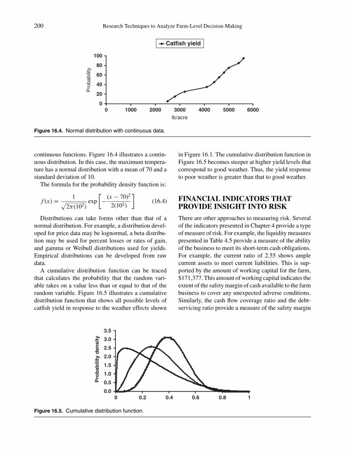
P1: SFK/UKS P2: SFK



0

20

40

60

80

100

6000500040003000200010000

Pro

babi

lity

lb/acre

Catfish yield

Figure 16.4. Normal distribution with continuous data.

continuous functions. Figure 16.4 illustrates a contin-uous distribution. In this case, the maximum tempera-ture has a normal distribution with a mean of 70 and astandard deviation of 10.

The formula for the probability density function is:

f (x) = 1√2π (102)

exp

[− (x − 70)2

2(102)

](16.4)

Distributions can take forms other than that of anormal distribution. For example, a distribution devel-oped for price data may be lognormal, a beta distribu-tion may be used for percent losses or rates of gain,and gamma or Weibull distributions used for yields.Empirical distributions can be developed from rawdata.

A cumulative distribution function can be tracedthat calculates the probability that the random vari-able takes on a value less than or equal to that of therandom variable. Figure 16.5 illustrates a cumulativedistribution function that shows all possible levels ofcatfish yield in response to the weather effects shown

0.0

0.5

1.0

1.5

2.0

2.5

3.0

3.5

0 0.2 0.4 0.6 0.8 1

Pro

bab

ility

den

sity

Figure 16.5. Cumulative distribution function.

in Figure 16.1. The cumulative distribution function inFigure 16.5 becomes steeper at higher yield levels thatcorrespond to good weather. Thus, the yield responseto poor weather is greater than that to good weather.

FINANCIAL INDICATORS THATPROVIDE INSIGHT INTO RISK

There are other approaches to measuring risk. Severalof the indicators presented in Chapter 4 provide a typeof measure of risk. For example, the liquidity measurespresented in Table 4.5 provide a measure of the abilityof the business to meet its short-term cash obligations.For example, the current ratio of 2.55 shows amplecurrent assets to meet current liabilities. This is sup-ported by the amount of working capital for the farm,$171,377. This amount of working capital indicates theextent of the safety margin of cash available to the farmbusiness to cover any unexpected adverse conditions.Similarly, the cash flow coverage ratio and the debt-servicing ratio provide a measure of the safety margin

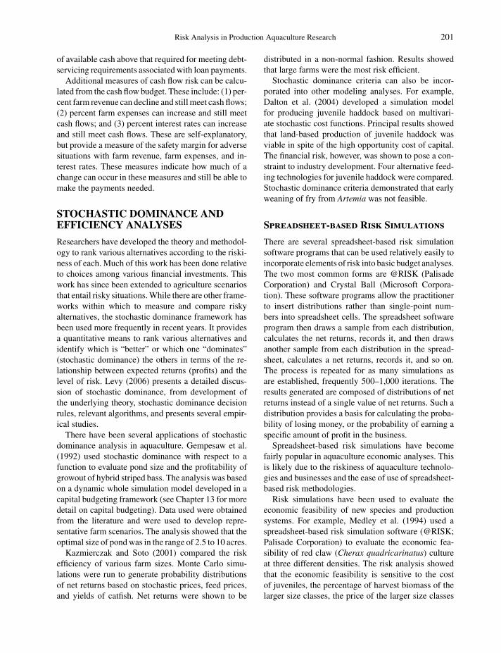
P1: SFK/UKS P2: SFK



of available cash above that required for meeting debt-servicing requirements associated with loan payments.

Additional measures of cash flow risk can be calcu-lated from the cash flow budget. These include: (1) per-cent farm revenue can decline and still meet cash flows;(2) percent farm expenses can increase and still meetcash flows; and (3) percent interest rates can increaseand still meet cash flows. These are self-explanatory,but provide a measure of the safety margin for adversesituations with farm revenue, farm expenses, and in-terest rates. These measures indicate how much of achange can occur in these measures and still be able tomake the payments needed.

STOCHASTIC DOMINANCE ANDEFFICIENCY ANALYSES

Researchers have developed the theory and methodol-ogy to rank various alternatives according to the riski-ness of each. Much of this work has been done relativeto choices among various financial investments. Thiswork has since been extended to agriculture scenariosthat entail risky situations. While there are other frame-works within which to measure and compare riskyalternatives, the stochastic dominance framework hasbeen used more frequently in recent years. It providesa quantitative means to rank various alternatives andidentify which is “better” or which one “dominates”(stochastic dominance) the others in terms of the re-lationship between expected returns (profits) and thelevel of risk. Levy (2006) presents a detailed discus-sion of stochastic dominance, from development ofthe underlying theory, stochastic dominance decisionrules, relevant algorithms, and presents several empir-ical studies.

There have been several applications of stochasticdominance analysis in aquaculture. Gempesaw et al.(1992) used stochastic dominance with respect to afunction to evaluate pond size and the profitability ofgrowout of hybrid striped bass. The analysis was basedon a dynamic whole simulation model developed in acapital budgeting framework (see Chapter 13 for moredetail on capital budgeting). Data used were obtainedfrom the literature and were used to develop repre-sentative farm scenarios. The analysis showed that theoptimal size of pond was in the range of 2.5 to 10 acres.

Kazmierczak and Soto (2001) compared the riskefficiency of various farm sizes. Monte Carlo simu-lations were run to generate probability distributionsof net returns based on stochastic prices, feed prices,and yields of catfish. Net returns were shown to be

distributed in a non-normal fashion. Results showedthat large farms were the most risk efficient.

Stochastic dominance criteria can also be incor-porated into other modeling analyses. For example,Dalton et al. (2004) developed a simulation modelfor producing juvenile haddock based on multivari-ate stochastic cost functions. Principal results showedthat land-based production of juvenile haddock wasviable in spite of the high opportunity cost of capital.The financial risk, however, was shown to pose a con-straint to industry development. Four alternative feed-ing technologies for juvenile haddock were compared.Stochastic dominance criteria demonstrated that earlyweaning of fry from Artemia was not feasible.

Spreadsheet-based Risk Simulations

There are several spreadsheet-based risk simulationsoftware programs that can be used relatively easily toincorporate elements of risk into basic budget analyses.The two most common forms are @RISK (PalisadeCorporation) and Crystal Ball (Microsoft Corpora-tion). These software programs allow the practitionerto insert distributions rather than single-point num-bers into spreadsheet cells. The spreadsheet softwareprogram then draws a sample from each distribution,calculates the net returns, records it, and then drawsanother sample from each distribution in the spread-sheet, calculates a net returns, records it, and so on.The process is repeated for as many simulations asare established, frequently 500–1,000 iterations. Theresults generated are composed of distributions of netreturns instead of a single value of net returns. Such adistribution provides a basis for calculating the proba-bility of losing money, or the probability of earning aspecific amount of profit in the business.

Spreadsheet-based risk simulations have becomefairly popular in aquaculture economic analyses. Thisis likely due to the riskiness of aquaculture technolo-gies and businesses and the ease of use of spreadsheet-based risk methodologies.

Risk simulations have been used to evaluate theeconomic feasibility of new species and productionsystems. For example, Medley et al. (1994) used aspreadsheet-based risk simulation software (@RISK;Palisade Corporation) to evaluate the economic fea-sibility of red claw (Cherax quadricarinatus) cultureat three different densities. The risk analysis showedthat the economic feasibility is sensitive to the costof juveniles, the percentage of harvest biomass of thelarger size classes, the price of the larger size classes

P1: SFK/UKS P2: SFK



of red claw crayfish, and the length of the productionseason.

Zucker and Anderson (1999) compared various al-ternative production and marketing scenarios with adynamic, stochastic model of a land-based summerflounder (Paralichthys dentatus) farming business. Themodel was developed using Microsoft Excel

R©(Mi-

crosoft Corporation, Washington, USA) software. Thesimulation model developed included submodels forthe production facility, for growth and biological pa-rameters, marketing, and a financial summary. Dataused were primarily from literature and expert opin-ion. Two selling strategies and six marketing strategieswere modeled along with various alternative scenariosthat included: (1) varying growth rates by 25%; (2)effects of a low interest rate of 2%; (3) advancementin system engineering that results in a 25% increasein density; and (4) change in policy that allows forpossession of fish smaller than 0.34 kg. Model resultsshowed that conditions for such a land-based flounderproduction system to be profitable included a locationnear a source of salt water, sales that targeted premiummarket outlets such as sushi markets, and developmentof adaptive market strategies.

Spreadsheet-based risk analyses have also been usedto identify key sources of risk for established aqua-culture species and technologies. Several studies useddata from shrimp farms in risk analyses. For exam-ple, Valderrama and Engle (2001) developed an anal-ysis of the financial risks of shrimp farming in Hon-duras with a stochastic simulation model using CrystalBallTM software (Decisioneering, Denver, Colorado).Data used were obtained from a survey of shrimp farmsin Honduras that included farms from 10 ha to over 400ha as well as an alternative semi-intensive technologyfor raising shrimp. Correlations identified in the sur-vey data for feed prices and farm sizes were used tolink six other variables (total seed costs, feed quantity,total full-time labor, total diesel costs, debt payment,and infrastructure depreciation). The primary sourceof risk in this situation was not price fluctuation butfluctuating yields. Certainty levels of achieving prof-its on various farm sizes and production technologieswere calculated.

Seijo (2004) used Crystal Ball© to develop a bioe-conomic model to estimate the risk of exceeding spec-ified limit reference points for shrimp aquaculture pro-duction. Particular emphasis was placed on assessingthe alternative timing of harvesting decisions. Resultsshowed that risk can be reduced by harvesting in 6–7 months. The model also showed which types of

financial indicators are affected the most by harvestingin other periods.

Martinez and Seijo (2001) further developed themodel to evaluate the economic effects of risk anduncertainty of various alternative water exchange andaeration rates in semi-intensive shrimp culture sys-tems. Particular sources of risk included: seed price,shrimp growth rate, survival rate, and shrimp prices.Results showed that the traditional production technol-ogy was more profitable than reducing water exchangeand increasing aeration levels. Nevertheless, the dif-ferences were small and, under the assumed risks, theprobability of achieving a positive net present valuewas high.

Martinez and Seijo (2001) developed an Excel-based bioeconomic model with a Bayesian decisionanalysis approach. The model was used to choose thecycling strategy for shrimp farms in Mexico, either a6–8 month production cycle or 2-, 3-, or 4-month pro-duction cycles with complete harvests. The two-cyclestrategy was a better option for the southern areas whilethe one-cycle strategy was better for the northern areas.

Pomerleau and Engle (2003) used a spreadsheet-based risk simulation analysis to evaluate the effectsof stochastic fluctuations of feed cost, feed conversionratio (FCR), yield, survival, and fish length on break-even costs of production data. Data used were froman experimental pond study. The lowest risk strategywas the medium stocking density. The risk analysisfurther showed that the probability of breakeven priceswas 0–9% of being above the stocker market price of$2.20/kg.

Hishamunda et al. (1998) developed a spreadsheet-based risk analysis of small-scale fish farming inRwanda. The add-in software program to Lotus 1-2-3, @Risk, was used to develop a simulation of fishfarming by cooperatives and by individual farmers.Labor was the major determinant of economic successon small-scale farms in Rwanda. Overall, the proba-bility of economic success was below 15% and netreturns to land and management were negative. More-over, fish production was riskier than production ofbeans and cabbages. Farms managed as cooperativeswere likelier to fail than were farms that were managedby individual farmers.

RISK PROGRAMMINGMODEL-BASED RESEARCH

Chapter 17 describes methods to develop whole-farmmodels with mathematical programming techniques,

P1: SFK/UKS P2: SFK



including methods of incorporating risk and stochasticelements into the analysis. This section will providea few examples of applications of risk programmingmodels in aquaculture.

Risk programming models have been used toevaluate new production technologies. For example,Hochmann et al. (1990) developed a stochastic dy-namic decision model to evaluate the potential of around pond technology for shrimp production. Themodel results provided an optimal stocking and har-vesting schedule for a shrimp pond that resulted indoubling net profits from shrimp production.

Other analyses have used risk programming tech-niques to evaluate management alternatives for es-tablished aquaculture industries such as shrimp andcatfish. For example, Valderrama and Engle (2002)developed a Target MOTAD risk programming modelof shrimp farming in Honduras based on survey datafrom commercial shrimp farms. Overall risk levelsmeasured were relatively low, primarily due to selec-tion of intermediate and low stocking densities duringthe rainy season. However, dry season production wasassociated with a relatively high degree of risk. Al-ternate farm plans were identified that further reducedrisk levels.

Engle and Hatch (1988) developed a Target MO-TAD risk programming model to compare alternativeaeration strategies for catfish production. Data usedincluded experimental data available from the litera-ture. Greater amounts of electric aeration on catfishfarms allowed farmers to increase stocking densitiesand feeding rates. However, these more intensive pro-duction levels entailed greater risk of losses frompower outages or other events that result in losses. Thestudy results identified the profit-maximizing choice ofaeration strategy for different levels of risk toleranceof farmers. Continuous nightly aeration was selectedmost often, but greater levels of concern of financialrisk resulted in selecting a less expensive type of elec-tric aerator.

OTHER SIMULATIONS AND RISKANALYSES

Arnason (1992) developed a dynamic optimizationmodel to develop optimal feeding and harvestingschedules for a variety of different growth response re-lationships. The analysis demonstrated that the profit-maximizing feeding paths may take a variety of dif-ferent shapes that depend on the shape of the growthfunction. The Arnason (1992) study was extended by

Heaps (1993) to demonstrate that, if fish growth isdensity-independent, then harvesting scheduling neednot account for culling fish before.

Jin et al. (2005) developed a simulation model toassess the risk of open-ocean aquaculture. The modelis based on an expected value-variance analysis of afirm-level investment–production model to simulateaquaculture growout, estimate the benefit–cost valuesof the project, and to calculate the risk premium for arisk-averse investor. The analysis included a case studyof open-ocean aquaculture of Atlantic cod (Gadusmorhua) in New England, USA. The analysis showedthat the risk level and the risk-aversion parameter wereinversely related to the investment level. Under condi-tions of uncertainty, the scale of aquaculture operationswould be smaller than with certainty of conditions.

Tveteras (1999) evaluated risky production tech-nologies on Norwegian salmon farms by examiningthe risk properties of inputs and patterns of technicalchange for both deterministic and risky parts of thetechnology. The analysis further examined how dif-ferent specifications of farm-specific effects, differentfunctional forms, and different estimators influencedthe empirical results. Results showed that increasingfeed and fish inputs increased risk while increasing la-bor inputs decreased risk. A risk preference functionwas developed for Norwegian salmon farming basedon panel data to estimate a Cobb-Douglas productionfunction. Absolute, relative, and downside risks foreach producer were calculated from the parametersestimated from the risk preference function. Salmonfarms were found to be risk averse and salmon farm-ers’ risk preferences exhibited decreasing absolute riskaversion.

RECORD-KEEPING

Risk analysis requires data on the variability of keyparameters. In aquaculture, these key parameters ofteninclude the price of the product, the price of feed, andthe yield (lb/acre of production). Thus, it is importantto maintain access to records of how the values of theseparameters fluctuate over time.

Records of prices of some types of aquaculture prod-ucts can be found in publicly available sources. Forexample, in the United States, prices paid to farm-ers of catfish and trout are available online from theU.S. Department of Agriculture. However, there areno long-term datasets of prices of other types of aqua-culture species. Even when there is a long-term indus-try dataset for prices, it is important for the farmer/

P1: SFK/UKS P2: SFK



0

10

20

30

40

50

60

70

–750

,000

–715

,000

–610

,000

–505

,000

–400

,000

–295

,000

–190

,000

–85,0

00

20,00

0

125,0

00

230,0

00

335,0

00

440,0

00

545,0

00

650,0

00

755,0

00

860,0

00

Fre

qu

ency

Figure 16.6. Frequency distribution of net returns for 256-acre catfish farm.

manager to maintain a record of the prices received foreach shipment of fish.

Net prices are even more important to track. De-ductions from the stated price will affect the overallprofitability of the business. Tracking the reasons forthe deductions may point to strategies to reduce theseover time or to decide to switch to another processingplant.

Tracking yields from ponds will provide a basis fromwhich to calculate the yield risk. If some ponds con-sistently produce lower yields than others over time,overall farm-wide yield risk can possibly be reducedby reworking those ponds or planting them in a differ-ent crop.

Similarly, recording total feed fed to each pond foreach year will allow the manager to track FCRs, over-all performance of various ponds, and how this perfor-mance varies from year to year.


The enterprise budget presented in Chapter 10(Table 10.2) was used as the basis for a risk simula-tion analysis using the Microsoft Excel add-in programCrystal Ball (Decisioneering, Denver, Colorado). Ta-ble 10.2 shows net returns to operator’s labor, manage-ment, and risk of $2,792 for the 256-acre catfish farm.

Stochastic distributions were entered into thespreadsheet for the following parameters: yield of cat-fish, price of catfish, feed prices, feeding rate, and

prices of fingerlings, labor, fuel (gas and diesel),electricity, repairs and maintenance, bird depredation,telephone expenses, office supplies, farm insurance,and legal/accounting expenses. Normal distributionswere used for the yield of catfish, fish prices, feed-ing rate, and feed prices. Triangular distributions wereused for prices of fingerlings, labor, and the othertypes of inputs. The simulations were run with 1,000iterations.

Figure 16.6 shows the frequency of net returns tooperator’s labor, management, and risk that resultedfrom the simulation analysis.

Mean net returns were −$4,577 ± $8,683 for the256-acre catfish farm. The profitability of making aprofit above total costs was 51% while the probabil-ity of covering all variable costs was 71%. Table 16.2shows the rank correlations of the contributions ofthe relative contributions of each stochastic parameteron overall risk. Yield clearly had the greatest effecton overall risk (0.89) and was followed by the priceof catfish (0.27). The analysis demonstrates the careand attention that must be paid to achieving consis-tent yields on the farm, from both a management andresearch perspective.


Zucker and Anderson (1999) used a dynamic stochas-tic model to develop recommendations for a newly

P1: SFK/UKS P2: SFK



Table 16.2. Rank Correlation Coefficients forthe Stochastic Parameters in the RiskSimulation Analysis of a 256-acre CatfishFarm.

ParameterRank correlation

coefficient

Yield 0.89Catfish price 0.27Feed price −0.21Feeding rate −0.19Farm insurance −0.07Repairs and maintenance 0.06Office supplies 0.04Electricity −0.03Fingerling price −0.03Fuel (gas and diesel) −0.03Telephone 0.02Salary 0.01Bird depredation 0.01Legal/accounting −0.01Second salary −0.01

emerging aquaculture technology, that of land-basedproduction of summer flounder. For a new startupaquaculture business, there are both production andmarketing risks that can determine the success or fail-ure of the new business. The model developed wasused to evaluate a series of scenarios. The scenariosevaluated included: (1) the effects of improvements inthe biological production that would result in 25% im-provements in the growth rates at the lower end of thedistribution and 5% improvement in the fastest growthrates expected; (2) effects of a low-interest loan rateof 2% on real estate and vehicle loans; (3) engineer-ing improvements that would increase the productioncapacity of the system by 25%; and (4) change in reg-ulations that would allow for fish smaller than 0.34 kgto be sold.

The least risky alternative, in terms of generatingprofits from the business, was to locate the businessnear a ready source of saltwater, sell to sushi chefswho prefer a medium-sized fish, and actively managethe business to adjust to market dynamics. The sce-nario that resulted in the greatest improvement wasthe policy option that would allow flounder farmersto sell a smaller fish, although all options consideredshowed some improvement.

SUMMARY

This chapter presents an overview of risk in aquacul-ture, discussing the various types of risk (production,marketing, and financial) and the difference betweenrisk and uncertainty. Risk measurements based oncalculating probabilities and probability densityfunctions are presented. Literature on the use ofspreadsheet-based risk simulations, stochastic dom-inance analysis, and risk programming model-basedstudies is summarized.

REVIEW QUESTIONS

1. What is risk and how is it different from uncer-tainty to economists?

2. List three major categories of risk and describeaquaculture examples of each.

3. What is commonly the relationship between riskand expected profits? Draw a graphical illustrationof this relationship.

4. How is risk measured? Describe several ways tomeasure risk.

5. What is a cumulative distribution function andhow is it interpreted?

6. Describe several financial indicators that can beused to interpret the level of risk for an aquaculturebusiness. Use examples from aquaculture.

7. What is a spreadsheet-based risk simulation andwhat output does it provide?

8. Name and describe two software programs thatcan be used to develop a risk simulation with aspreadsheet program.

9. Describe some uses of risk programming mathe-matical programming models.

10. Describe several situations for which a risk anal-ysis would be a more appropriate type of analysisthan a deterministic analysis.

REFERENCES

Arnason, Ragnar. 1992. Optimal feeding schedulesand harvesting time in aquaculture. Marine Re-source Economics 7(1):15–35.

P1: SFK/UKS P2: SFK



Dalton, Timothy J., Kate M. Waning, and Linda Kling.2004. Risk efficient juvenile haddock productionsystems: an ex-ante recursive stochastic approach.Aquaculture Economics and Management 8(1/2):41–59.

Engle, Carole R. and Upton Hatch. 1988. Economic as-sessment of alternative aquaculture aeration strate-gies. Journal of the World Aquaculture Society19(3):85–96.

Gempesaw, Conrado M., Richard Bacon, and Ferdi-nand F. Wirth. 1992. Economies of pond size forhybrid striped bass growout. Journal of the WorldAquaculture Society 23(1):38–48.

Heaps, Terry. 1993. The optimal feeding of farmedfish. Marine Resource Economics 8:89–99.

Hishamunda, Nathanael, Curtis M. Jolly, and UptonHatch. 1998. Evaluating and managing risk in small-scale fish farming in a developing economy: an ap-plication to Rwanda. Aquaculture Economics andManagement 2(1):31–38.

Hochman, P.S. Leung, L.R. Rowland, and J. Wyban.1990. Optimal scheduling in shrimp mariculture:a stochastic growing inventory problem. AmericanJournal of Agricultural Economics 72:382–393.

Jin, Di, Hauke Kite-Powell, and Porter Hoagland.2005. Risk assessment in open-ocean aquaculture:a firm-level investment-production model. Aquacul-ture Economics and Management 9:369–387.

Kazmierczak, Richard F., and Patricia Soto. 2001.Stochastic economic variables and their effect onnet returns to channel catfish production. Aquacul-ture Economics and Management 5(1/2):15–36.

Knight, Frank H. 1921. Risk, Uncertainty, and Profit.1964 Edition. New York: Augustus M. Keley.

Levy, Haim. 2006. Stochastic Dominance: InvestmentDecision Making Under Uncertainty. New York:Springer Science Business Media.

Martinez, Jose A. and Juan Carlos Seijo. 2001. Eco-nomics of risk and uncertainty of alternative waterexchange and aeration rates in semi-intensive shrimpculture systems. Aquaculture Economics and Man-agement 5(3/4):129–145.

Medley, Paul B., Robert G. Nelson, Upton Hatch,David B. Rouse, and Gerard F. Pinto. 1994. Eco-nomic feasibility and risk analysis of Australianred claw crayfish Cherax quadricarinatus aqua-culture in the southeastern United States. Jour-nal of the World Aquaculture Society 25(1):135–146.

Pomerleau, Steeve and Carole R. Engle. 2003. Produc-tion of stocker-size channel catfish: effect of stock-ing density on production characteristics, costs, andeconomic risk. North American Journal of Aquacul-ture 65:112–119.

Seijo, Juan Carlos. 2004. Risk of exceeding bioeco-nomic limit reference points in shrimp aquaculturesystems. Aquaculture Economics and Management8(3/4):201–212.

Tveteras, Ragnar. 1999. Production risk and pro-ductivity growth: some findings for Norwegiansalmon aquaculture. Journal of Productivity Anal-ysis 12(2):161


Valderrama, Diego and Carole R. Engle. 2002. Eco-nomic optimization of shrimp farming in Honduras.Journal of the World Aquaculture Society 33(4):398–409.

Zucker, David A. and James L. Anderson. 1999. A dy-namic, stochastic model of a land-based summerflounder Paralichthys dentatus aquaculture firm.Journal of the World Aquaculture Society 30(2):219–235.

P1: SFK/UKS P2: SFK


17Whole-Farm Modeling of Aquaculture

INTRODUCTION

Economic analysis of aquaculture frequently has fo-cused on examining the economic consequences ofspecific changes that might be made on the farm basedon a new experiment that has yielded what appear to bebeneficial results. Enterprise budgets, partial budgets,and cost analyses have been commonly used. However,these types of analyses are limited in scope in that theyexamine only one enterprise (enterprise budget), onesmall change on the farm (partial budget), or costs as-sociated with a specific production activity (cost anal-ysis). In many cases, the analysis is developed on thebasis of a single pond as the unit of analysis.

These types of analyses are useful as long as theyare interpreted correctly. Incorporating some cost andreturn elements into basic production research doesprovide insights into the results and can suggest impli-cations.

These types of analyses, however, are limited inthat many variables from across the farm may affectwhether or not the farmer can implement the new re-search results. The number of ponds, availability andskill level of the workforce, access to capital for oper-ating or for additional investment, availability of ad-equate types and suitability of equipment, credit ca-pacity of the farm business, and regulatory constraintsmay prevent new technologies or new research resultsfrom being adopted or from being feasible on farms.Enterprise budgets, partial budgets, and cost analysesdo not allow these types of constraints to be consideredin the analysis.

An enterprise is part of a greater farming systemthat involves sometimes complex interactions acrossthe entire farm. Ignoring these interactions may leadto farm plans that are not feasible or are not realistic.

Whole-farm models incorporate the availability ofresources, constraints, and their interactions acrossthe entire farm. Biological, economic, and financialfactors are integrated into one analysis. Whole-farmmodels can be used to compare the economics ofadopting new technologies on a farm, to identify theoptimal set of production practices for that partic-ular farm, or to identify which types of resourcesare the most constraining to that particular farmbusiness.

There are two basic broad categories of whole-farm modeling: whole-farm budgeting and mathe-matical programming models. Whole-farm budget-ing is similar in some ways to developing anenterprise budget, with the difference that the costsand revenues are developed for the entire farm. Math-ematical programming models are more flexible thana whole-farm budget and provide a comprehensivemodel that results in a more complex set of resultsthat demonstrate how to optimize the use of the farm’sresources.

Development of a whole-farm budget relies primar-ily on farm records of costs and returns. If a farmermaintains appropriate records and develops balancesheets and income statements each year, there is littledifficulty in converting these numbers into a whole-farm budget. If the farmer wishes to consider changesfor the next year, the effects of those changes canbe estimated for an “end-of-year” whole-farm bud-get that shows the effect on farm profits. The pri-mary disadvantage of whole-farm budgeting is thatbudgets are cumbersome mechanisms for examininga variety of levels associated with different technolo-gies and changes. For example, a farmer looking atchanging stocking densities on his/her farm wouldhave to choose exactly which densities to use in whichponds prior to developing the whole-farm budget. Ifhe/she then decides that additional densities need tobe analyzed, an entirely new farm budget will need


207

P1: SFK/UKS P2: SFK



to be developed. The degree of labor and financialconstraints to the farm business must be set prior todeveloping the budget and new budgets must be de-veloped for each different level of labor or financialconstraint.

Mathematical programming models, on the otherhand, allow for inclusion of a variety of levels of dif-ferent changes being considered for the farm. If stock-ing density is the major change being considered, themodel can include 5, 10, or more different densities.Moreover, the model can be developed to include dif-ferent stocking densities of different sizes, species, orstrains of fish. Different levels of availability of oper-ating and investment capital, terms of lending, vary-ing availability of degrees of skill of labor along withvarying prices of inputs can be modeled in mathe-matical programming models. However, developmentof mathematical models requires a great deal of data.Each option included in the model requires completedata. If few data are available on the various alterna-tives and levels desired for the analysis, a whole-farmbudget may be the only option available. It is betterto develop a simpler model from reliable records, thento develop a more sophisticated model with too fewdata. Training and skill are required to develop usefulmathematical programming models.

This chapter discusses both whole-farm budget pro-cedures and mathematical programming model analy-ses in aquaculture. The various types of analyses arecompared and contrasted.

WHOLE-FARM BUDGETING

A whole-farm plan outlines the production activitiesfor the farm and identifies the resources needed toproduce this set of activities. The whole-farm budgetcompiles the resource requirements and expected costsand returns for the combination of amounts of com-modities selected as the best combination for the farmbusiness.

The bottom line of the whole-farm budget is theprojected net farm income. If various scenarios areconsidered, the net farm income can be compared toselect the specific plan that results in the greatest netfarm income.

The structure of a whole-farm budget is similar tothat of an income statement. The various sources ofrevenue are itemized by type of crop to be produced.Variable and fixed costs for the entire farm are esti-mated. Total costs are subtracted from total revenue tocalculate net farm income.

Mechanics of Constructing aWhole-farm Budget

Development of a whole-farm budget begins with aninventory of resources. These include the land avail-able, buildings, wells, ponds, and other production fa-cilities, a marketing or grading shed, equipment avail-able, access to both investment and operating capital,labor, and management. It is important to specify de-tails on the type, quality, and quantity of each typeof resource. Pond sizes, number, volumes, and sizesof vats and tanks, all need to be specified. The abilityto borrow additional capital must be assessed realisti-cally. The lack of credit capacity can limit the adoptionof new technologies and limit the ability of the farmerto make needed upgrades to more efficient equipment.Liquidity problems can arise if input prices increaserapidly and unexpectedly and the farmer has no capac-ity to acquire additional operating capital.

Labor resources must be assessed as well. The levelof skill required for the types of enterprises selected forthe farm business must be specified. Management skillmust be assessed as well. Age, experience, manage-ment performance, special skills, and any weaknessescan be important factors.

When resources available to the farmer have beenidentified, the enterprises to be included on the farmmust be selected. Decisions should include the speciesto be raised and whether to raise foodfish crops or in-termediate crops of fingerlings or stockers. Enterprisebudgets must be developed for each enterprise to beincluded on the farm. The enterprise budget specifiesthe resources required, costs and revenue, and grossand net margins for each unit of production.

The next step is to determine how much of each en-terprise to raise on the farm. The key is to identify thebest use of the resources available and which combi-nation of enterprises will result in the highest profitsgiven the set of resources available to the farm.

The whole-farm budget then estimates the expectedrevenue and expenses. Cash inflow, outflow, and liq-uidity should be evaluated along with the effects ofvarious combinations of enterprises on profits and liq-uidity. Other options for changing the farm plan, suchas adopting a new technology or expansion or contrac-tion of the farm business should be considered. Finally,the exact amount of resources required for the optimalfarm plan should be detailed.

Whole-farm budgets can be used to projectoutcomes for proposed changes on the farm. Netreturns and liquidity can then be compared across

P1: SFK/UKS P2: SFK


Whole-Farm Modeling of Aquaculture 209

the various combinations considered. Net cash flowcan be projected for each combination considered byadding expected farm and off-farm revenue for eachplan under consideration. Cash farm income fromnonfarm work and investments are then added to totalcash inflows. Cash farm expenses and cash outlays toreplace capital assets and debt payments all constitutecash outflows. Total farm cash outflows are subtractedfrom cash inflows to obtain net cash flows for thebudget for each whole-farm plan developed.

MATHEMATICAL PROGRAMMING

Mathematical programming is a computationalmethod to allocate limited resources to maximize profitor minimize costs. It is a mathematical technique thatuses a systematic procedure to find the best possi-ble enterprise combination. It allocates resources totheir best possible uses to achieve a given objective,given the limitations and restrictions on the use of eachtype of resource. It can be used at the farm, industry,or regional level. The word “programming” refers toplanning and not developing computer code. However,computers are used to solve large mathematical pro-gramming models to find the “optimal” (best or mostprofitable) plan.

There are many uses of mathematical program-ming models. They can be used to (1) identify profit-maximizing combinations of scarce resources (labor,land, feed, fry) for production of a given species; (2)allocate land to particular crops; (3) identify the bestallocation of scarce resources for production of dif-ferent species; (4) develop plans for the most efficientuse of labor and machinery; (5) identify the least-costingredients of a diet to meet specified nutritional re-quirements and formulate least-cost rations for live-stock; (6) identify least-cost geographic sources fromwhich fry and raw materials should be purchased; or(7) identify the best allocation of output among geo-graphic markets.

Fundamental Concepts UnderlyingMathematical Programming Models

Linear programming (LP) models essentially trace aproduction possibilities curve (for more details on theeconomic concept of a production possibilities curve,see (Baumol and Blinder 1999)) with linear segments.A production possibilities curve shows a series ofpoints where combinations of production activities arefeasible, given the quantities of resources available andthe quantities required for each type of crop.

Hybrid striped bass

Catfish

Capital

LaborLand

A

B

C

D

Figure 17.1. Graphical illustration of the concept of lin-ear programming.

Figure 17.1 illustrates the fundamental concept thatunderlies LP with a simplified two-dimensional graph.Only two decision variables can be represented in suchtwo-dimensional graphs. Hybrid striped bass and cat-fish production quantities are graphed on the axes. Thelines represent the linear equations of requirements forthe resource constraints of land, labor, and capital. Thepoints A, B, C, and D define the area called the feasibleregion. Any combination of tilapia and catfish activi-ties on or within this area is feasible given the resourcerestrictions or constraints. The optimal solution isfound by identifying the line of equal gross margin thatjust touches one of the vertex points (A, B, C, or D).

The optimal plan that is generated from a LP modelconsists of the number of acres of ponds or the head offish stocked needed to maximize profits. This combi-nation of enterprises then needs to be used to developthe financial and economic statements that correspondto that optimal plan.

Structure of Basic LP Model

For whole-farm planning, a mathematical program-ming model typically maximizes an objective functionsubject to specified constraints. LP models (in whichthe equations in the model are linear) are most com-monly used because they do not require as much dataas some of the other types of models.

The LP tableau is a table that organizes theinformation for a LP model. Table 17.1 demonstrates

P1: SFK/UKS P2: SFK


Tab

le17

.1.

Sim

ple

Mod

elof

Fis

hFa

rmin

Tha

iland

(inT

haiB

aht)

.

Mor

eIn

tens

ive

Sell

tilap

iaE

xten

sive

inte

nsiv

etil

apia

Cat

fish

Sell

Con

stra

int

poly

cultu

repo

lycu

lture

mon

ocul

ture

cultu

reL

ocal

lyV

illag

eD

istr

ict

Cat

fish

type

RH

S

Obj

ectiv

efu

nctio

n−2

,395

−2,5

31−2

,179

,032

−52,

402

3040

3027

0M

AX

Pond

bala

nce

11

11

0L

E4

Tila

pia

fry

00

25,0

000

0L

E10

0,00

0C

atfis

hfin

gerl

ings

00

013

2,40

00

LE

150,

000

Ure

aba

lanc

e0

1,33

21,

719

859

0L

E10

0,00

0T

SPba

lanc

e0

872

1,12

556

20

LE

100,

000

Lim

e0

766

988

494

0L

E10

0,00

0A

nim

alm

anur

e96

01,

920

12,4

138,

288

0L

E10

0,00

0Fe

edfo

rfr

y0

297.

629

7.6

00

LE

100,

000

Feed

for

grow

out

25.4

25.4

1,47

6.5

211,

061

0L

E50

0,00

0L

abor

for

grow

out

1942

.75

5029

40

LE

100,

000

Lab

orfo

rha

rves

ting

44

1282

,794

0L

E10

0,00

0Po

ndm

aint

enan

ce55

02,

550

2,55

02,

550

0L

E10

0,00

0M

arke

ting

(Bt/k

g)lo

cal

046

90

00

LE

100,

000

Mar

ketin

gtil

apia

fart

her

00

6,02

20

0L

E10

0,00

0M

arke

ting

catfi

sh0

00

82,7

940

LE

100,

000

Ope

ratin

gca

pita

l0

LE

2,50

0,00

0A

nnua

linv

estm

ent

capi

tal

1,60

53,

210

6,42

06,

420

0L

E5,

000,

000

Tila

pia

prod

uctio

nfo

rlo

cals

ales

−437

.50

01

0L

E0

Tila

pia

prod

uctio

nfo

rvi

llage

sale

s0

−1,8

750

10

LE

0

Tila

pia

prod

uctio

nfo

rdi

stri

ctsa

les

00

−60,

222

−6,0

221

0L

E0

Cat

fish

prod

uctio

n0

00

01

0L

E0

LE

,les

sth

anor

equa

lto;

RH

S,ri

ght-

hand

side

valu

e.

P1: SFK/UKS P2: SFK



Right-handSide (RHS)

Maximize Z = c1x1 + c2x2 + … + cnxn

Subject to (s.t.) a11x1 + a12x2 + … + a1nxn < b1

a21x1 + a22x2 + … + a2nxn < b2

am1x1 + am2x2 +…+ amnxn < b3

Decision variables

Figure 17.2. Mathematical form of a linear program-ming model.

a tableau for an LP model for an aquaculture businessin Thailand.

LP models include a linear objective function thatdescribes mathematically the objective of the farm planto be developed and the decision variables or activitiesto be optimized (Figure 17.2). This equation consistsof the sum of revenue-generating opportunities withthe costs subtracted from the revenue generated. Theobjective function for farm plans usually maximizesnet returns on the farm.

Decision variables, the variables whose values willbe calculated by the model, are selected and defined.Each decision variable represents a particular farm en-terprise or a particular level of production of a farmenterprise. An example could be the number of pondsto allocate to hybrid striped bass production in eithermonoculture or a specific polyculture combination.Each different production level for each enterprise isspecified as a separate decision variable. These levelsmay represent various stocking densities, various lev-els of aeration usage, different sizes of ponds, or someother production or management system.

The resources that limit how much and what canbe produced are modeled as constraints in the model.Constraints represent the limitations or restrictions onthe number of units of an activity or variable that can beput into production, given the level of resources avail-able. For example, farms have only a certain numberof ponds available and the farm plan cannot allocateactivities to more ponds than are available (unless themodel allows for the possibility of an activity to buildadditional ponds). Typical constraints include land, la-bor, fingerlings, and capital. Credit capacity used inthe plan cannot exceed the farm’s credit or exceedthe maximum on the line of credit. The combination

of activities selected cannot require more labor thanthe size of the workforce unless additional activitiesare added to allow additional labor to be hired. Con-straints typically include the resources available, butcan also include market constraints. For example, ifthe market for hybrid striped bass for the farm is only100,000 lb/year, then it is important to specify in themodel that no more than 100,000 lb of hybrid stripedbass can be sold in a year.

For the model to be a LP model, the objective func-tion and the constraints must be expressed as linearequations. These must also be deterministic and notcontain random elements. The decision variables arecontinuous and non-negative (they must assume posi-tive values).

There are certain assumptions that underlie LP.These include separability, proportionality, divisibil-ity, and non-negativity. Separability implies that thereis no interaction among the decision variables andallows the objective function to be written as thesum of several functions. For example, a modelthat includes purchases of hatchery-raised and wildpostlarvae of shrimp is built upon the assumptionthat greater purchases of wild postlarvae do not re-duce purchases of hatchery-raised shrimp. There arespecial techniques that can be used to relax thisassumption.

The proportionality assumption implies that thereare no economies of scale. If proportionality exists,the value of each constraint function is directly pro-portional to the value of each decision variable. Forexample, as larger quantities of postlarvae are pro-duced, the unit price remains the same if proportion-ality exists. Thus, it would not be correct to assumethat unit prices fall if larger quantities of shrimp post-larvae are produced. Special techniques have beendeveloped to introduce economies of scale in LPmodels.

Divisibility allows for resources and decision vari-ables to be used in fractional quantities. Techniques(integer programming) have been developed for deci-sion variables that require integer values. For example,a farmer cannot stock 0.3 ponds; when he or she stocksfish into a pond, the entire pond is stocked.

Non-negativity assumptions require that all decisionvariables are either zero or positive. Decision variablesand resource constraints are finite in LP models. More-over, single-valued expectations are used because allparameters are known with certainty.

Data requirements for a mathematical program-ming model begin with an inventory of the resources

P1: SFK/UKS P2: SFK



available. Potential cropping alternatives must beidentified. Then, data will be required on the technicalcoefficients of production. These coefficients aredeveloped from the resource requirements for eachunit of enterprise included in the model. Net returnsare estimated for each cropping alternative or activity.Because the equations in a mathematical program-ming model are inequalities, the maximum quantity ofeach that is available to the farmer must be specifiedand recorded as the right-hand side value (RHS).

Objective Function

The objective of a mathematical programming modelis to either maximize or minimize something. In a farmplanning model, the objective typically is to maximizenet returns. The gross margin of each unit is multi-plied by the number of units selected to include in thefarm plan. These are summed to calculate the total netreturns. Each enterprise (shrimp, tilapia fingerlings,tilapia foodfish, etc.) must be included as a term in theequation for the objective function.

Table 17.1 presents the tableau for a LP model de-signed to develop an optimal farm plan for a fish farmin Thailand. The farmer wishes to maximize net re-turns, thus the objective function is to maximize netreturns. This objective function can be expressed asfollows:

Maximize Z = 0X1 + 0X2 + 0X3 + 0X4 + 30X5

+ 40X6 + 30X7 + 27X8 (17.1)

Activities and Decision Variables

In Table 17.1, the fish farmer is considering raisingeither tilapia or catfish. Tilapia enterprises consideredare either extensive or intensive polyculture or inten-sive monoculture. Moreover, tilapia can be sold locallyat lower prices, in villages at slightly higher prices, orat district markets at even higher prices. Thus, the deci-sion variables are to produce tilapia in either extensiveor somewhat more intensive polyculture, in intensivemonoculture, to raise catfish intensively, to sell cat-fish, or to sell tilapia in either local, village, or districtmarkets. Mathematically, the decision variables can beexpressed as:

X1 = tilapia production in extensive polyculture in a1-ha pond

X2 = tilapia production in more intensive polyculturein a 1-ha pond

X3 = high-intensity tilapia monoculture in a 1-ha pond

X4 = catfish production in monoculture in a 1-ha pondX5 = tilapia sales in local markets, in kgX6 = tilapia sales in village markets, in kgX7 = tilapia sales in district markets, in kgX8 = catfish sales, in kg

Constraints

There is always a limit to the quantity of resourcesavailable to the farmer. The value of this limit restrictswhat the farmer can and cannot do and different levelsof this value can alter the profit-maximizing solution.The resource constraints in a LP model are developedas technical coefficients that equate to the amount ofthe particular resource needed to produce one unit ofthat enterprise. The equation then consists of the tech-nical coefficients of the resources required for pro-duction of that enterprise multiplied by the number ofponds selected to be used for production of that en-terprise. The sum of the quantities of resources usedfor each enterprise must be less than or equal to thetotal amount of that resource available. The total num-ber available is specified as the RHS value for eachresource and constitutes the constraint or limit on itsuse. Small programs can be solved by hand, but pro-grams with large numbers of enterprises or with manyrestrictions require a computer to solve.

The first row of the tableau is the objective functionand includes the gross margin coefficients for each ac-tivity. The following rows represent the resource con-straints and balance rows. Each column represents adecision variable and the values in each row show howmuch of each resource is needed for each unit of theactivity. Other columns represent sales activities andthe RHS shows how much of that resource is available.

In the example provided in Table 17.1, the con-straints include the availability of ponds, tilapia fryand catfish fingerlings, fertilizers (urea, triple super-phosphate or TSP, lime, and animal manure), feed(for fry and for growout), labor (for growout and forharvesting), pond maintenance, marketing (tilapia lo-cally or farther and catfish), capital (operating and in-vestment, and fish production transfer rows). In thisexample, each production activity (extensive tilapiapolyculture, more intensive tilapia polyculture, high-intensity tilapia production, and high-density catfishproduction) would each require at least one pond andwould be added into the solution in units of a pond.For example, the first row in Table 17.1 is the pondconstraint.

P1: SFK/UKS P2: SFK



Each type of production system is modeled as aunit of one pond and all technical coefficient valuesare calculated on a per-pond basis. The numeral 1 foreach production activity in the pond constraint rowindicates that if selected in the optimal solution, thenthe corresponding amounts of other resources will beentered proportionally. The RHS value of 4 representsthe four ponds available on the farm. This constraintwould be expressed mathematically as:

1X1 + 1X2 + 1X3 + 1X4 + 0X5 + 0X6

+ 0X7 + 0X8 ≤ 4 (17.2)

The next row is the tilapia fry resource. The intensivetilapia monoculture activity stocks 25,000 fry per pondand up to 100,000 fry (RHS value) are available for theentire farm. Similarly, the catfish monoculture activityrequires 132,400 catfish fingerlings per pond. The nextrows are the fertilizer resources of urea, TSP, lime, andanimal manure. The number in each column representsthe amount of fertilizer or lime needed for each pondin each alternative. The next row is the amount of feedrequired and then labor, and maintenance costs. Asanother example of how the constraints are expressedmathematically, the constraint of labor required forgrowout would be expressed mathematically as:

19X1 + 42.75X2 + 294X3 + 50X4 + 0X5 + 0X6

+ 0X7 + 0X8 ≤ 100,000 (17.3)

Marketing constraints follow that indicate how manypounds of product can be sold in each type of mar-ket outlet. Operating capital requirements for each al-ternative and annual investment capital are next. Thefollowing rows (tilapia production for sale, tilapia pro-duction for village sales, and tilapia production for dis-trict sales) are transfer rows to move production of fishfrom production to sales.

The fish production transfer rows link the produc-tion activities to the sales activities. For example, thetilapia production for village sales constraint would beexpressed mathematically as:

0X1 − 1,875X2 + 0X3 + 0X4 + 0X5 + 1X6

+ 0X7 + 0X8 ≤ 0

Redundancy in constraints can increase the computingtime. Redundancy occurs when a decision variable cansatisfy more than one constraint. In computer models,redundancy does not have to be eliminated from theproblem.

Right-Hand Side

The constant terms that appear on the RHS of theconstraint equations are referred to as the right-handside values or RHS values. These values represent theamount of the resource available on the farm. RHSvalues must clearly be non-negative also.

Solving an LP Model

In order to solve the inequality constraints in the model,the equations must first be converted to equalities.Thus, the Equation 17.1 becomes

1X1 + 1X2 + 1X3 + 1X4 + 0X5 + 0X6

+ 0X7 + 0X8 + s1 = 4

The s1 variables are referred to as slack variables.For less-than-or-equal-to inequalities, the slackvariables appear with positive signs and are calledpositive slacks, or surplus variables. Negative slackvariables are associated with greater-than-or-equal-toinequalities.

Originally developed for the solving of multisectoraleconomy-wide models, the general algebraic model-ing system (GAMS) (Brooke et al. 1998) was adoptedas a standard tool by economists who work in ap-plied optimization. GAMS is a high-level languagethat uses concise algebraic statements easily read byboth modelers and computers, are easily modified,and easily moved from one computer environmentto another. It contains a series of solvers that usevarious algorithmic methods to approach a wide ar-ray of problems from linear and nonlinear, mixedinteger, mixed integer nonlinear, and other types ofproblems.

Small mathematical programming models can besolved with Microsoft Excel. The practical applicationin this chapter presents how to set up and run smallmodels in Excel.

An unbounded solution is one that has an infiniteboundary, or no upper limit. Without an upper limit,the problem cannot be solved; the computer will con-tinue to increase the number of units to be produced inan infinite manner. An unbounded solution indicatesthat the model was not developed properly. Modelsthat have severe resource restrictions such that posi-tive values cannot be found for the decision variablesare referred to as infeasible.

P1: SFK/UKS P2: SFK



Interpreting the Output

The printed output includes the value of the objectivefunction. Information provided on the rows includesstatus indicators of BS (row not a limiting factor), LL(solution lies on lower limit of constraint), or UL (so-lution lies on upper limit of the constraint). The valuesindicating the quantities selected for the solution andthe amount of each resource used as well as slack val-ues are indicated in the printed solution.

Dual values, including shadow prices and reducedcosts, are also reported in the output. Shadow pricesare the amount by which total gross margin wouldbe increased if one more unit of that resource wereavailable. For enterprises, the shadow price showshow much the gross margin would be reduced byforcing one unit of an enterprise into the plan. Ifresources are not used completely, the shadow price iszero. However, if the resource is used up completely,then the shadow price indicates whether additionalunits of that resource should be acquired. The decisionmaker should compare the cost of acquiring anotherunit of resource with the shadow price. If the shadowprice is higher, its value is greater than its cost and it isworthwhile to acquire more. However, if the shadowprice is less than its cost, then it is not profitable toacquire more.

The reduced costs indicate what the effect ongross margins would be by using another unit of anenterprise that was not included in the plan. Onlyenterprises that were not included in the optimal planwill have a reduced cost other than zero. The outputalso includes the input costs entered for each variablethat entered the objective. The reduced cost indicatesthe amount by which the input cost would need tochange for the optimal solution to be positive for thatvariable (reduced cost is zero for values selected forthe optimal solution).

Sensitivity Analysis, Thresholds,Basis Changes

The optimal solution, the combination of activities thatmaximizes profits, is known as the basis. The basisconsists of the set of variables that enter into the opti-mal solution. Changes in the RHS values or changesin the price, cost, or other technical coefficients canresult in changes in the basis. Sensitivity analyses thatsystematically vary key parameter values will demon-strate what price or cost levels will result in a changein the basis. Thus, the range of values over which thebasis remains stable is identified. These types of sen-

sitivity analyses are often referred to as parametricprogramming.

Other Types of MathematicalProgramming Models

LP models have been the most commonly used typesof mathematical programming models. However, thereare a number of other types of mathematical program-ming models. Examples include integer, quadratic,goal programming, multiperiod, transshipment, andrisk programming models (E-V, MOTAD, Target MO-TAD), among others.

Integer programming refers to restricting certain pa-rameter values to integer values as opposed to the con-tinuous values that are a requirement of LP models. Agoal programming model specifies an objective func-tion as a target or goal instead of either maximizingor minimizing one specific objective. Thus, in goalprogramming, the objective is to minimize deviationsfrom a target.

When parameters are not known with certainty, theassumption of single-valued expectations is relaxedand risk programming models are developed. Riskmodeling in economics is based on the assumption thatthe probability distributions of the risky parameters areknown with certainty. The risk model, then, representsthe decision-maker’s response to parameter risk (Mc-Carl and Spreen 1997). The optimal plan developedmay not necessarily be the best for each possible typeof event, but is intended to establish a position that isrobust across the entire set or distribution of parametervalues.

One of the first types of risk programming models,the mean-variance, or E-V model was first developedby Markowitz (1959) to identify an optimal invest-ment strategy for a portfolio. The variables indicatethe amount of funds invested in each alternative in-vestment option. Each is constrained by a total fundsconstraint, or the total amount of investment capitalavailable. One assumption behind this approach is thatinvestors do not place all their funds in the highestyield option; thus, a LP model would not be appropri-ate because linear models would put all the funds inthe option that generates the highest yields.

In an E-V model, a risk aversion coefficient ismultiplied by the variance of total income andsubtracted from the expected income. The E-V modelis based on the assumption that decision-makers tradeexpected income for lower levels of risk (reducedvariance). The model can be solved for varyinglevels of risk aversion parameters. Each new solution

P1: SFK/UKS P2: SFK



reduces the variance of total returns, lowering risk,but also reducing net returns.

The E-V model is a quadratic programming problemthat is more difficult to solve than a linear program.Software programs are available to solve it, but datarequirements can still be difficult.

The difficulties involved in developing quadraticprogramming models led to the development of linearapproximations to the E-V problem. The minimizationof total absolute deviations, or MOTAD, model definesvarious states of nature related to the deviation frommean income. The model then characterizes the trade-offs between the expected income and the absolutedeviation of income.

Roy (1952) introduced an approach referred to asa safety-first model. This approach assumes that de-cision markers will first select plans to assure a givensafety level for income, typically set as a level of in-come that will cover production costs. Low levels ofsafety (high risk) correspond to the profit-maximizingLP solution. However, as the safety level increases,risk decreases, but the expected returns also decrease.

Tauer (1983) extended the safety-first model by al-lowing negative deviations from the safety level. A tar-get income level is set and variables are included thatindicate negative deviations from income. The maxi-mum average income shortfall is set at the safety level.

In a Target MOTAD model, allowing for large devia-tions results in a profit-maximizing LP solution. How-ever, as the allowable deviation is reduced, solutionsare diversified. Thus, risk reductions are accompaniedby larger deviations.

Sequences of decisions can be modeled as optimiza-tion problems with dynamic programming. Dynamicprogramming methods were developed by Bellman(1957) and Bellman and Dreyfus (1962). Dynamicprogramming models trace an optimal path from aninitial state to another state. In dynamic programming,states are defined that indicate a particular point orconfiguration. Stages are the transitions from one stateto another. Policies are the sets of actions that equateto a particular objective.

To solve dynamic programming models, recurrencerelations are constructed that relate the various states.The recurrence relations are then used to calculate anoptimal policy.

RECORD-KEEPING

Many of the types of records needed to develop awhole-farm model are those required also for enter-prise budgets. A whole-farm model begins with a com-

plete inventory of resources available to the farm, fromland to types of ponds and facilities.

Information on the various alternative types of pro-duction options then must be collected. Keeping thisinformation on hand over time provides a basis forfuture consideration. Data over time of prices of theproducts under consideration is used to project pricetrends and to identify any correlations that can be takenadvantage of to reduce risk by diversifying production.


Table 17.2 illustrates the tableau for the 256-acre cat-fish farm whose owner is considering adding a hybridstriped bass enterprise to the farm. This example prob-lem will be solved using the Excel solver program andFigure 17.2 illustrates how to lay out the tableau to besolved with the Excel solver.

The objective function is to maximize profits forthe farm. The decision variables included productionof catfish for growout or fingerlings or growout ofhybrid striped bass for foodfish. Other decision vari-ables included the possibility to purchase fingerlings orto grow fingerlings on farm. The constraints includeda pond constraint and the necessary transfer rows totransfer fingerlings from either the fingerling purchaseactivity or the on-farm fingerling production activityto the growout activity, and to transfer hybrid stripedbass produced from the hybrid striped bass productionactivity to the hybrid striped bass sales activity.

The first line in the Excel solver version of thetableau contains 0s. The first line is the one that Excelwill change to find the solution that will indicate thenumber of ponds (production activities) or pounds offish to be sold (sales activities) assigned to each de-cision variable in the optimal solution. The next rowis the pond constraint. Each pond production variable(catfish foodfish growout, catfish fingerling produc-tion, or hybrid striped bass growout) is based on aunit of one 10-acre pond. Thus, a “1” is entered inthe pond constraint row for each of these activities.The fingerling transfer row shows the number of cat-fish fingerlings needed for one 10-acre catfish pond(56,900). In the column of the on-farm fingerling pro-duction activity, the number of fingerlings producedin one 10-acre pond is recorded (−93,665). The pos-sibility to purchase fingerlings is recorded as −1. Thefoodfish transfer row shows the number of poundsof catfish foodfish produced in one 10-acre pond(−45,000). The foodfish are transferred to the catfishsales activity with the one in the sell catfish column.The hybrid striped bass foodfish transfer row transfers

P1: SFK/UKS P2: SFK



Table 17.2. Tableau for 256-acre Catfish Farm.

Growcatfish

from 5”fingerlings

On-farmfingerlingproduction

Buyfingerlings

GrowHSB

Sellcatfish

SellHSB RHS

Number of pondsto use

0 0 0 0 0 0

Ponds 1 1 0 1 0 0 0 LE 25Fingerling transfer 56,900 −93,665 −1 0 0 0 0 LE 0Foodfish transfer −45,000 0 0 0 1 0 0 LE 0HSB foodfish

transfer0 0 0 −45,000 0 1 0 LE 0

Marketingconstraints

0 0 0 0 0 1 0 LE 100,000

Objective function −22,943 −16,192 −0.07 −46,307 0.7 1.50 0

RHS, right-hand side value; HSB, hybrid striped bass.

the −45,000 lb of hybrid striped bass foodfish from thehybrid striped bass production to sell hybrid stripedbass sales (1). Finally, the marketing constraint for hy-brid striped bass limits the amount of hybrid stripedbass foodfish to the size of the market for the product,with a “1” in that row.

The RHS values indicate the amount of each re-source available. For the pond constraint, there are 2510-acre ponds on the farm. The marketing constraintfor hybrid striped bass is 100,000 lb. The objectivefunction indicates both costs associated with each de-cision variable and the revenue to be obtained fromeach activity. The production costs for catfish food-fish production are approximately −$22,943 for each10-acre pond. One 10-acre pond in catfish fingerlingproduction costs −$16,192 per pond. Each fingerlingpurchased costs −$0.07 while one 10-acre pond ofhybrid striped bass foodfish costs −$46,307 per pond.Each pound of catfish sold generates $0.70 of revenuewhile hybrid striped bass bring $1.50 per pound sold.

For the solver to function, a separate column isneeded next to the RHS values. In this column, the“sumproduct” function is used to multiply the row ofcells that will be the values to change to identify theoptimal amount by each individual row of constraints.The sumproduct function must also be used to multi-ply the row of changing cell values by the values inthe objective function.

After setting up the tableau, the solver can be usedin Excel to find the profit-maximizing combination ofactivities. The solver is available as an add-in func-tion under the “Data” tab in Excel 2007 and under

“Tools” on the Excel menu on older versions of Excel.Clicking on the solver brings up a dialogue box withseveral smaller boxes to fill in. The first box to fill in isthe target cell. This is the cell that will record the netreturns value for the farm that results in the optimalsolution that shows the combination of activities thatresults from solving the LP model. This is the cell withthe sumproduct function associated with the objectivefunction. The next box asks for the cells that will havechanging values and that will identify the number ofeach activity to be included. The next step is to identifythe constraints. The cell with the sumproduct formulafor each constraint row is indicated as the constraint.The symbol for less-than-or-equal-to or greater-than-or-equal-to or equal to is selected as appropriate andthen the cell that contains the RHS value is indicated.Before running the model, the options button shouldbe selected. In the options dialogue box, the “linearmodel” and “non-negative” boxes should be checked.After clicking “OK” to return to the previous dialoguebox, it is time to click “solve.” Excel will then indi-cate whether a feasible solution was found. If found,various report options can be selected.

Table 17.3 shows the optimal solution for the catfish-hybrid striped bass model. In the base solution, 23ponds were put into catfish foodfish production andtwo ponds were put into hybrid striped bass growoutproduction. Fingerlings were purchased and the farmsold 1,025,000 lb of foodfish catfish and 100,000 lb ofhybrid striped bass, for a total net returns of $144,801.

The sensitivity report option shows a reduced costof −$13,457 for on-farm fingerling production. This

P1: SFK/UKS P2: SFK


Tab

le17

.3.

Bas

eS

olut

ion

for

256-

acre

Cat

fish

Farm

.

Cat

fish

prod

uctio

nfr

om5”

finge

rlin

gs

On-

farm

finge

rlin

gpr

oduc

tion

Buy

finge

rlin

gsG

row

HSB

Sell

catfi

shSe

llH

SBR

HS

Num

ber

ofpo

nds

tous

e23

01,

296,

056

21,

025,

000

100,

000

Pond

s1

10

10

025

LE

25Fi

nger

ling

tran

sfer

56,9

00−9

3,66

5−1

00

00

LE

0Fo

odfis

htr

ansf

er−4

5,00

00

00

10

0L

E0

HSB

food

fish

tran

sfer

00

0−4

5,00

00

10

LE

0H

SBm

arke

ting

cons

trai

nts

00

00

01

100,

000

LE

100,

000

Obj

ectiv

efu

nctio

n−2

2,94

3−1

6,19

2−0

.07

−46,

307

0.7

1.50

151,

281

151,

281

RH

S,ri

ght-

hand

side

valu

e;H

SB,h

ybri

dst

ripe

dba

ss.

P1: SFK/UKS P2: SFK



indicates that, if fingerlings had been produced on apond on the farm that gross margins would have beenreduced by $13,457. Shadow prices were $4,290 forponds and $1.12 for hybrid striped bass sales. Thismeans that gross margins would have increased by$4,290 if another pond had been available, $1.12 ifan additional pound of hybrid striped bass could havebeen sold.


Engle and Valderrama (2004) used an economic op-timization model to evaluate several different prac-tices that had been recommended as best managementpractices for shrimp farming in Central America. Themodel was used to identify several options that in-creased farm profits by improving production efficien-cies while also reducing net quantities of nutrientsdischarged as effluents. The most effective practiceswere to reduce water exchange rates and the use offeed trays. These are technologies that can be com-bined and practiced by a wide array of farm sizes.

SUMMARY

This chapter presents methods to develop whole-farmplanning models. Whole-farm modeling reveals po-tential conflicts in the use of resources on the farmand identifies a pattern of resource use that will max-imize farm profits. Both whole-farm budgeting andmathematical programming can be used. Whole-farmbudgeting is simpler to use, but each option to be con-sidered requires a separate whole-farm budget. Mathe-matical programming, on the other hand, is a very flex-ible planning tool, but requires a great deal of skill todevelop. Mathematical programming models includelinear, goal, risk, and dynamic programming options.

REVIEW QUESTIONS

1. Why are whole-farm models of value?

2. Explain the relative advantages and disadvantagesof whole-farm budgets and mathematical pro-gramming models.

3. Describe the process of developing a whole-farmbudget.

4. List the major types of uses of mathematical pro-gramming models.

5. What are the specific features that make a mathe-matical programming model be a LP model?

6. Give an aquaculture example of a LP model thatis unbounded.

7. Describe the major components of a LP model(objective function, decision variables, con-straints, and RHS values).

8. Explain what information is provided by shadowprices and reduced costs in the output of a LPmodel.

9. What are goal and risk programming? Give severalexamples of how LP models can be converted intogoal or risk programming models.

10. Describe what dynamic programming can be usedfor and how a dynamic programming model isdeveloped.

REFERENCES

Baumol, William J. and Alan S. Blinder. 1999. Mi-croeconomics: Principles and Policy. 7th ed. Mason,OH: Southwestern Publishing Company.

Bellman, Richard E. 1957. Dynamic Programming.Princeton: Princeton University Press.

Bellman, Richard E. and Stuart E. Dreyfus. 1962. Ap-plied Dynamic Programming. Princeton: PrincetonUniversity Press.

Brooke, Anthony, David Kendrick, Alexander Mier-aus, and Richard E. Rosenthal. 1998. GAMS UserGuide. Release 2.50. San Francisco: The ScientificPress.

Engle, Carole and Diego Valderrama. 2004. Economiceffects of implementing selected components of bestmanagement practices (BMPs) for semi-intensiveshrimp farms in Honduras. Aquaculture Economicsand Management 8:157–177.

Markowitz, Harry M. 1959. Portfolio Selection. NewYork: John Wiley and Sons.

McCarl, Bruce and Thomas Spreen. 1997. Appliedmathematical programming using algebraic sys-tems. Available at agrinet.tamu.edu.

Roy, A.D. 1952. Safety-first and the holding of assets.Econometrica 20:431–449.

Tauer, Loren W. 1983. Target MOTAD. Ameri-can Journal of Agricultural Economics 65(3):606–610.

P1: SFK/UKS P2: SFK


18Managing Government Policies and

Regulation in Aquaculture Businesses

INTRODUCTION

Aquaculture worldwide is developing at a rapid paceduring a time of increased regulatory pressure. The in-creased focus and attention on aquaculture comes froma number of sources, but much of it has stemmed fromthe pressure from environmentalist and public advo-cacy groups. Many of these groups have targeted aqua-culture. They see aquaculture emerging as an industryacross the world and hope to influence its developmentand evolution because they expect aquaculture to playan ever-increasing role in the world’s future food sup-ply. These groups have hired lawyers and other person-nel who mount well-orchestrated initiatives to pressureregulators to develop new policies.

Increasing numbers of countries have developedpolicies, plans, and regulations related to aquaculture.The fisheries and aquaculture sectors have been in-creasingly integrated into national policy documents.New regulations that result from these policies can leadto a variety of management changes that add new costsfor aquaculture businesses. Moreover, the costs of re-acting to the various types of allegations from publicadvocacy groups are not borne by the public agencies,but must be addressed by the businesses that are af-fected. These types of costs are not normally includedin typical financial statements. Yet, if the owners andmanagers of aquaculture businesses do not engage inthe public and regulatory discussions related to thedevelopment of new regulations, the end result maybe new laws, ordinances, and regulations that increasecosts or force farm-level changes that turn the businessinto an unprofitable or infeasible one.

The issues involved rarely are resolved permanently.While new issues may emerge as time goes on, manysurface into prominence for a period of time, then arepushed into the background for a while only to resur-face farther down the road. This chapter discusses theseissues and their effects on the economics of aquacul-ture businesses.

COMPLYING WITH EXISTINGREGULATIONS

All businesses must comply with existing regulations.These regulations include local ordinances, state andfederal policies, and, increasingly, international regu-lations. Compliance with such a variety of permits canbe costly in terms of the time required, hiring special-ized personnel, and paying fees. Maintaining the per-mits entails additional costs to keep up with changesin regulations and permitting.

Local regulations are highly variable and specific tothe particular area. Most aquaculture businesses wereconstructed originally on farmland. However, as ur-ban areas expand, more and more aquaculture busi-nesses find themselves within city limits. As zoningordinances change, and restrictions related to zoningemerge, there is potential for conflicts to emerge withexisting aquaculture farms. Zoning has also becomerelevant to mariculture businesses in coastal and off-shore waters. Some parts of the world (Spain, UnitedStates) have experimented with mariculture parks orzones that restrict aquaculture activities to that area.Canada, Malaysia, Sri Lanka, and Australia have alldeveloped zoning programs for aquaculture, primarilyin coastal and marine areas.

Table 18.1 lists examples of the variety and preva-lence of various types of state regulations in the UnitedStates related to aquaculture. Most states in the United


219

P1: SFK/UKS P2: SFK



Table 18.1. State Regulations and Permits Required for Aquaculture-Related Activities.

Category Description Number of states

Regulations Licensing and permitting for aquaculture 40 states and territoriesPossession of aquatic animals for aquaculture 30 statesWater supply 26 states and territoriesNon-native species 22 states and territoriesDischarge control and protection of fish and wildlife 16 states and territoriesProcessing 15 statesLeasing of submerged public lands 13 statesDischarges (other than federal NPDES permits) 11 statesUse of coastal areas 2 statesDepuration for shellfish 2 statesInspection Arizona

Permits 24 states and territoriesDischarges (NPDES) 44 states and 1 territoryTideland use, including dredging 5 statesFood quality sanitation and safety 3 statesOther permits 7∗

∗Include aquaculture, certification, land use and development, gear or equipment, and disposal of mortalities.

States (40 states and territories) require some sort ofpermit or license to run an aquaculture business. Ofthese, 30 states and territories have regulations relatedspecifically to the possession of aquatic species foraquaculture. For processing, 15 states have regulationsrelated to processing the products from aquacultureand 13 states have regulations related to leasing sub-merged public lands. A few states have regulations re-lated to inspection (1), shellfish depuration (2), conser-vation districts (1), and the use of coastal areas (2).

Twenty-four states and territories require varioustypes of permits for aquaculture businesses (Table18.1). Common permits required include food san-itation, quality, and safety, tideland use (includingdredging), and discharges. Other less frequently usedpermits are for gear or equipment (1 state), disposalof mortalities (2 states), land use and development(1 state and 1 territory), animal damage permits (2states), food quality sanitation and safety (3 states),shellfish certification guidelines (1 state), and anaquaculture permit (1 state).

There are a variety of federal regulations thataquaculture business owners must comply with (Ta-ble 18.2). The primary agencies involved with federalpermits for aquaculture include U.S. Army Corps ofEngineers, U.S. Department of Commerce, and theU.S. Fish and Wildlife Service. The U.S. Army Corps

of Engineers (USACE) regulates the construction ofdams and levees in dredged and filled sites throughSection 404 permits. The USACE is authorized to is-sue these permits under the Federal Water PollutionControl Act of 1972, as amended by the Clean Wa-ter Act of 1977, and Water Quality Act of 1987. TheFederal Coastal Management Zone Act of 1972 reg-ulates proposed federal activities that affect a state’scoastal zone. Section 10 of the Rivers and Harbor Actof 1989 regulates the creation of obstructions not au-thorized by Congress to navigable waterways of theUnited States. The Federal Sanitation Standards forFish Plants of the Department of Commerce providesfor inspection of processing plants and facilities andgrades aquaculture products for quality assurance. TheU.S. Fish and Wildlife Service regulates activities thatmight affect endangered or threatened species or theirhabitat through the Endangered Species Act of 1983.The Lacey Act amendments of 1981 are also enforcedby the U.S. Fish and Wildlife Service. Under the LaceyAct, it is unlawful to import, sell, acquire, or purchasefish, wildlife, or plants taken, possessed, transported orsold in violation of U.S. or Indian law or in interstate orforeign commerce. The Migratory Bird Act (enforcedby the U.S. Fish and Wildlife Service) regulates theuse of lethal control methods on migratory birds thatcause aquaculture crop losses.

P1: SFK/UKS P2: SFK


Managing Government Policies and Regulation in Aquaculture Businesses 221

Table 18.2. Federal Regulations Related to Aquaculture.

Category Specific title of regulatory authority Agency

Construction of dams and leveesfor dredged and filled sites

Section 404 of the Federal WaterPollution Control Act of 1972,amended by Clean Water Act of 1977,and Water Quality Act of 1987

U.S. Army Corps of Engineers

Use of coastal zones Federal Coastal Zone Management Actof 1972

Use of navigable waters Section 10 of the Rivers and Harbors Actof 1989

Processing plants and gradingstandards

Federal Standard Sanitation U.S. Department of Commerce

Standards for Fish PlantsActivity that might affect

endangered or threatenedspecies or their habitat

Endangered Species Act of 1973 U.S. Fish and Wildlife Service

Interstate transportation of fishand wildlife

Lacey Act Amendments of 1981 U.S. Fish and Wildlife Service

Bird depredation Migratory Bird Treaty Act U.S. Fish and Wildlife Service

INFLUENCING THE OUTCOMES OFREGULATORY PROCESSES

Aquaculture has grown to a size that has attractedthe attention of numerous nongovernmental organi-zations and regulatory bodies. Yet, many individualsin many countries including the United States have lit-tle knowledge or understanding of aquaculture. This isparticularly problematic when aquaculture is such a di-verse industry, producing nearly 500 different speciesof plants and animals in a wide array of different pro-duction systems (FAO 2000–2008). The likelihood ofthe individuals who develop new rules and regulationshaving some background or experience in aquacul-ture is very low. Regulators often are faced with highworkloads, stringent deadlines, and have little time toresearch and study the industries that they are chargedwith regulating. At the same time, most regulatory au-thorities are charged to base their rule making on thebest available science. How are regulators to find, un-derstand, and integrate the best available science forevery industry for which they are expected to developnew rules?

The only answer to this question is that it is in thebest interest of the aquaculture industry to positionitself to be the primary source of information for reg-ulators, the media, and the public. Individual farmersfrequently do not have the time to mount public re-lations campaigns on their own, much less to providethe level of detailed information that is needed by reg-

ulators. However, they can join and participate in thetrade association that is most closely associated withtheir products.

Producer associations have played an increasinglyimportant role in aquaculture development and regula-tion. These producer groups can be small, village-levelgroups, or international organizations. Participation ina trade association such as those listed in Table 18.3 isnecessary for several reasons. Trade associations canhave a major influence on regulatory decisions by in-sisting that there be an adequate scientific basis for therule, that the rules developed be reasonable, rational,and not overly burdensome financially. Informationpresented by trade associations can counterbalance thenegative media reports that pressure regulatory agen-cies to adopt new regulations for aquaculture.

The power and influence of a trade association is di-rectly related to the size of its membership. The morestakeholders that an association represents, the moreinfluence it has with which to negotiate. If an associa-tion has a sufficient dues-paying membership, it maybe able to afford to hire lobbyists, pay travel expensesto have representatives at crucial meetings in differentlocations, and participate in key workshops and events.

Active involvement in a trade association entailscosts associated with dues and attendance at associa-tion meetings. These constitute business costs in an eraof increasing regulation. As a member of an associa-tion, one is in the position of serving as representative

P1: SFK/UKS P2: SFK



Table 18.3. Examples of Aquaculture TradeAssociations.

Type of tradeassociation Name of trade association

International Global Aquaculture AllianceWorld Tilapia Association

Regional Federation of EuropeanAquaculture Producers

National Aquaculture Association ofCanada

Arkansas Bait and OrnamentalFish Growers Association

Association of Chilean SalmonFarmers

Catfish Farmers of America(U.S.)

Finnish Fish Farms AssociationIcelandic Fish Farmers and Sea

RanchersIrish Aquaculture AssociationNational Aquaculture Association

(U.S.)Norwegian Fish Farmers

AssociationStriped Bass Growers AssociationU.S. Trout Farmers of America

(U.S.)Provincial/State British Columbia Salmon

Farmers Association

on various task forces and working groups that provideinput to various rule-making efforts.

Every rule-making effort in the United States in-volves different periods of public comments. Both in-dividuals and associations have opportunities to submitcomments during these official periods. Coordinatingkey messages with trade associations is most effective.

In addition to participating in trade associations, in-dividual businessmen can engage in the rule-makingeffort through the political process. Politics is the sys-tem within which a democratic society “converses”about its priorities, choices, and makes decisions.Elected officials must be kept informed of the conse-quences to their constituents of various policies underconsideration. However, to have credibility, it is crit-ical that any input or information provided to electedofficials be well researched, credible, and defensible.

The first step is to get to know the appropriate electedofficials. Inviting members of the political delegation

to visit farms, contributing to campaigns, and attendingfund-raisers are all ways of developing a relationshipthat provides a path of communication to ensure thatone’s elected officials have the best possible and mostaccurate information on the aquaculture industry.

EXAMPLE OF BENEFITS OFENGAGING IN THE REGULATORYPROCESS: THE ENVIRONMENTALPROTECTION AGENCY EFFLUENTSRULE OF 2004

On June 30, 2004, the Administrator of the Environ-mental Protection Agency (EPA) of the United Statessigned the final rule for aquaculture. This signaturefollowed a 3-year rule-making period that was uniquein several respects. Firstly, it was the final rule devel-oped under a court-ordered consent decree, and it wasdeveloped with the engagement of a National TaskForce that not only included both EPA officials andstaff but also representatives of various sectors of theaquaculture industry as well as university and agencyscientists (Westers, 2000).

The backdrop to this rule included an initialevaluation of aquaculture by EPA in the early 1970s(Whitman et al. 2002). At that time, EPA did notpropose any regulations because the emphasis atthat time was directed toward sectors that dischargedeffluents that contained toxic metals and organics.In 1973, EPA proposed and implemented NationalPollutant Discharge Elimination System (NPDES)permit application rules for aquaculture. The NPDESpermits are required for farmers that discharge at least30 days/year (warmwater farms) or that produce lessthan 100,000 lb/year. For coldwater species, permitsare required for farms that discharge more than30 days/year and produce more than 20,000 lb/year.

The Clean Water Act provides for development ofeffluent limitation guidelines for point sources of pol-lution. In 1992, following a lawsuit by the NaturalResources Defense Council, a Consent Decree wassigned by the court. The Consent Decree required theEPA to set a timetable for the development of effluentlimitation guidelines for designated industries. In theoriginal list of industries, Rule #12 was the industrialcontainer cleaning industry. In late 1999, EPA askedthe court to substitute aquaculture for the industrialcontainer cleaning industry. The reasons given by EPAwere: (1) the only relevant guidance was more than20 years old; (2) the aquaculture industry had changedin terms of the species raised and the industrial

P1: SFK/UKS P2: SFK



processes employed; and (3) that states had identi-fied aquaculture as a common cause of water qualityimpairment on the 305b and 303b lists.

Scrutiny of the 305b and 303d lists by aquacul-ture scientists raised a number of questions. For exam-ple, substances such as mercury, arsenic, pesticides,and metals were listed as the cause of impairmentfrom aquaculture in Louisiana, California, and Ohio.Such substances are not used in aquaculture produc-tion. Moreover, a number of pesticides will kill fish,crustaceans, and other aquatic organisms and are notused on aquaculture farms. Moreover, a number ofthe major aquaculture-producing states were absentfrom the list all together. If aquaculture were a majorsource of impairment, the greatest impacts would beexpected to be visible in the major production states.A follow-up survey by the North Carolina Departmentof Agriculture showed that the 305b and 303d listsprovided by the states were compiled by listing alltypes of industries present in the watershed, withoutindication of which industry was responsible for thecontamination. Moreover, the survey documented thatstates considered existing regulations adequate to han-dle any effluent problems associated with aquaculture.

A National Aquaculture Effluents Task Force wasformed by the Joint Subcommittee on Aquaculture tosupport a nationally coordinated, systematic process toidentify and report the best available and appropriatescience and data related to discharges from aquacul-ture. The task force included representatives from var-ious aquaculture trade associations. The involvementof the more than 180 industry representatives and sci-entists provided a thorough sounding board for EPA ona wide variety of technological alternatives that werediscussed by EPA.

The EPA process for effluent limitation guidelines isbased on establishing mandatory production processesfor treating effluent discharges (Environmental Pro-tection Agency 2006). Essentially, EPA searches fortechnological alternatives that reduce the levels of dis-charge without causing an excessive number of busi-nesses to cease operations. EPA staff members have notraining in aquaculture. They typically work throughcontractors who carry out the analyses required, but thecontractors frequently do not have direct experience inthe businesses under consideration. Moreover, the spe-cific analyses prescribed for agency use may not coversome of the more relevant impacts and consequencesof the rule.

As an example of the work done by the Task Force,Engle et al. (2005) showed that the three effluent treat-

ment options under consideration (each option referredto a set of treatment options) would all cause small andmedium-sized trout farms to go out of business. Theanalysis also showed that, while large farms would stillhave positive net returns under the options proposed,their option would cause the probability of being prof-itable to fall from 84% without any additional treat-ments to 10–11%, depending on the options selected.Moreover, the mathematical programming model de-veloped demonstrated a high level of sensitivity toincreased requirements for operating and investmentcapital. No additional effluent treatments were fea-sible for the options proposed, due to the additionalinvestment capital required. The models showed thatimposing new effluent treatment options forced farmsto take raceways out of production to put them into ef-fluent treatment. This was due to the investment capitalrequired, limited access to capital by many trout farm-ers, and competing uses for land in trout farming areasthat have driven land prices in these areas upward.

Emerging Policy and RegulatoryIssues

There are a number of policy and regulatory issues thatare emerging but are not yet well developed enough tobe able to estimate the economic and financial costsinvolved. The following descriptions will present anoverview of economic and financial considerations re-lated to emerging policies related to trade, biosecurity,certification, aquatic nuisance species (ANS), and foodsafety issues.

TRADE ISSUES

Increasing globalization has had dramatic effects onaquaculture worldwide. The total volume of seafoodtraded worldwide was 108 million metric tons in2005. A high percentage of the most frequently tradedseafood products, such as salmon and shrimp, is fromaquaculture.

The increase in trade volume has been accompaniedby an increase in trade conflicts. The trade conflictshave resulted in a number of antidumping accusationsand lawsuits. The World Trade Organization providesfor antidumping suits to protect against sales of prod-ucts at unfairly low prices. All countries have somesorts of tariffs that have been imposed on some othercountry. Many include agricultural products and mostinclude some type of tariffs or regulations related toimported fish and fish products (World Trade Organi-zation 2008).

P1: SFK/UKS P2: SFK



Table 18.4. Examples of Trade Disputes in Aquaculture.

Species Country

Petition initiated Against Date

Salmon United States Norway 1988United States Chile 1997European Union Norway 1999

Swimming crab United States Venezuela, Thailand, Indonesia,Mexico

2000

Crawfish United States China 1994Basa/tra United States Vietnam 2002Mussels United States Canada 2001Shrimp United States (shrimp fishermen) Ecuador, Brazil, India, Thailand,

China, Vietnam2003

Many trade conflicts have involved salmon, partic-ularly as the farm-raised salmon industry has grownworldwide (Table 18.4). Some of the earliest conflictswere between the United States and Norway in the1980s. These were followed by conflicts between theUnited States and Chile in 1997, and the EuropeanUnion and Norway in the early 1990s. Blue crab im-ports into the United States from Venezuela, Thai-land, Indonesia, and Mexico were disputed in 2000.Increased imports of crawfish into the United Statesfrom China in 1994 prompted an antidumping petitionand subsequent countervailing tariffs.

The most recent trade conflicts in aquaculture haveinvolved the U.S. catfish industry and imports ofbasa/tra (Pangasius sp.) from Vietnam. The U.S. cat-fish industry filed an antidumping petition in 2002 andantidumping tariffs were imposed on Vietnam in 2003.After falling in 2002–2003, exports of basa/tra have in-creased again, although at a slower rate than their ex-ports to other countries. The import data reflect growthin the number of countries exporting basa/tra to theUnited States. Whether this reflects production fromthose countries or transshipment (sales through a thirdcountry to avoid countervailing tariffs) is unknown.

The United States and Canada have experiencedtrade conflicts over mussels imported into the UnitedStates from Prince Edward Island. In 2003, an an-tidumping petition was filed by shrimp fishermenand processors against shrimp growers from Ecuador,Brazil, India, Thailand, China, and Vietnam.

Trade conflicts, particularly antidumping petitions,involve substantial sums of capital. The legal fees in-volved in filing these petitions often amount to mil-

lions of U.S. dollars. Many aquaculture industries aretoo small to be able to afford such expensive litiga-tion. Some antidumping petitions have been filed byprocessors rather than growers and some of the costsinvolved have been paid by trade associations. Regard-less of the source of capital, the costs become substan-tial and eventually, in one form or another, add cost tothe farms and production units.

Biosecurity, as related to fish and other aquatic ani-mals has been an issue of growing concern and inter-est. Increased globalization and trade have increasedthe potential to spread aquatic pathogens across theglobe. Transmission of pathogens (such as whirlingdisease of trout and infectious salmon anemia virusof coldwater fish species) has been monitored and, insome cases, regulated, since the 1960s. However, lessattention has been paid to the transmission of warmwater fish pathogens, until recent years.

The Office International des Epizooties (OIE)(World Organization for Animal Health) regulates thespread of pathogens worldwide. The OIE AquaticCode was first developed in 1995. The OIE requiresthat fish health inspections be done for the interstatetransport of live fish and maintains a list of pathogensfor which aquatic animals must be inspected. Thehealth certificates issued must indicate the absence ofthese pathogens.

Recent outbreaks such as that of spring viremia ofcarp in the United States (2002) and, of viral hem-orrhagic septicemia (VHS) in the Great Lakes and inEurope in more recent years have heightened aware-ness of aquatic biosecurity issues in the United States.The United States Department of Agriculture-Animal

P1: SFK/UKS P2: SFK



Plant and Health Inspection Service (USDA-APHIS)is the regulatory authority responsible for control andsurveillance of aquatic pathogens. With the VHS out-break in the Great Lakes, USDA-APHIS is the regula-tory authority responsible for control and surveillanceof aquatic pathogens. With the VHS outbreak in theGreat Lakes, USDA-APHIS first issued an EmergencyOrder and then an Interim Rule related to transporta-tion of live fish. The rules prohibited the shipment ofVHS-susceptible species of live fish from states whereVHS had been detected, unless the fish had been in-spected and found to be free of VHS. This rule contin-ues to evolve over time.

To comply with this rule, farmers and live fish dis-tributors must have fish inspected. There are provisionsfor both farm-level (requires a two-year history) andlot inspections (every shipment must be tested). The to-tal annual expense to the farm business is much higherfor lot inspections due to the much higher total numberof inspections to be done. The cost of inspections in-cludes fees to veterinarians to collect the samples andthe costs for the diagnostic laboratories to conduct theanalyses. The costs and logistics of complying withinspections must be included in planning, monitoring,and financial analysis of the farm business.

In addition to the USDA-APHIS federal regulation,individual states in the United States have adoptedadditional regulations to prevent the introduction ofVHS into their states. These regulations vary consid-erably from state to state in terms of the species offish to be tested, the numbers to be tested, the fre-quency of inspections, and the pathogens to be testedfor. Aquaculture business owners who ship live fishin the United States must familiarize themselves withthese regulations and position themselves to have im-mediate access to changes in these regulations.

Some segments of aquaculture have developed cer-tification programs as a means to avoid delays that mayoccur due to changing regulations pertaining to biose-curity and the interstate shipment of live fish. Onesuch example is the Arkansas Baitfish CertificationProgram. To be certified under this program the farmmust have a two-year history of testing that shows thefarm is free of the diseases identified in the program(spring viremia of carp, infectious pancreatic necro-sis, and viral hemorrhagic septicemia, among others).Each farm is sampled twice a year by a licensed veteri-narian and samples tested for a variety of pathogens byan APHIS-approved laboratory. Certificates are issuedby the Arkansas State Department of Agriculture-StatePlant Board on paper that cannot be copied. Inspectors

of the State Plant Board inspect each farm in the certi-fication program twice a year to check for the presenceof Aquatic Nuisance Species (ANS) that are prohibitedin the program (zebra mussels, bighead carp, and silvercarp, among others). The program includes a fee paidto the Arkansas Department of Agriculture in additionto the veterinarian and laboratory testing fees.

Certification

There has been a dramatic increase in the number ofcertification programs for aquaculture in the last sev-eral years. The impetus for these programs stems pri-marily from concern on the part of major retailerslike Wal-Mart, Tesco, and Carrefour to maintain orimprove their reputation, competitiveness, and marketshare, in reaction to consumer concerns and to reducerisk of recalls, regulatory action, and poor quality. Re-calls result in significant losses in terms of sales andin damages to a company’s reputation. Lawsuits byenvironmentalist groups have resulted in an increasein use of certification programs by large retailers todemonstrate their commitment to environmental sus-tainability.

Growing reports of adulterations in seafood prod-ucts from China and Vietnam (antibiotics, fungicides,and melamine) have raised issues for congressionaland the Food and Drug Administration (FDA) actionin the United States. The end result is likely to beincreasing federal inspection and regulation.

Certification programs have been developed as aproactive response to these situations. Certificationprograms have focused on some of the key issuessuch as Hazard Analysis and Critical Control Point(HACCP), food and feed safety, food security, qual-ity, environmental impact and sustainability, traceabil-ity, inspection, auditing, third-party verification, andcertification by the Global Aquaculture Association(GAA), the World Wildlife Federation (WWF), Euro-Retailer Produce Working Group, the Irish QualityEco-Mussel Standard, and others. Each program isdesigned differently. For this reason, the Food andAgriculture Organization of the United Nations (FAO)has initiated a process to develop standards for certi-fication programs. Some, like the Irish Quality Eco-Mussel Standard is a single-species standard whilethe GAA/ACC is for multiple species. Most certifi-cation programs rely upon some type of third-partycertification. Companies such as the Aquaculture Cer-tification Council (used by GAA), SureFish, Inc. ofSeattle, Washington, and others have been developed

P1: SFK/UKS P2: SFK



to provide this service. EUREPGAP began in 1997by the Euro-Retailer Produce Working Group, drivenmostly by British retailers. EUREPGAP evolved intoGLOBALGAP in 2007 in response to the growinginterest from producers and retailers worldwide. TheGAA/ACC program includes a variety of componentsthat range from food safety, sanitation, good manu-facturing practices, environmental sustainability, ef-fluents, community involvement, and traceability.

All certification programs entail cost to the pro-ducer, although the amount of the cost varies. Whatis not clear is to what extent this cost can be passedthrough to the consumer. There is no clear researchthat indicates that consumers generally are willing topay higher prices for product that has been certified asenvironmentally sustainable. There are what appear tobe small segments of consumers who will pay morebut as of 2008, it does not appear to be a substantialconsumer segment.

It is difficult to judge the point at which it is worththe cost to enter a certification program. Depending onthe specific nature of the program, there is a risk to theproducer in addition to the cost. The risk consists of theprobability that a disease, ANS, or other problem maybe found during a routine inspection. This risk needs tobe weighed against potential advantages. If a primarysales customer begins to require participation in a cer-tification program, a farmer or processor may have nochoice. In other situations, it may be possible to turnthe certification program to a marketing advantage.These trade-offs, particularly whether there is a way touse certification to expand into new markets or to de-velop a competitive edge over competitors in existingmarkets must be weighed against the costs and risks.

Exotic and non-native species have become a ma-jor issue affecting aquaculture. The concern is thatnon-native species will out-compete native species thatwill result in a priceless loss of biodiversity throughhomogenization. Once a species is lost, that loss is for-ever. In the United States, there are an estimated 185non-native species of which 75 have become estab-lished. In addition, there are 316 species that are nowfound outside their native ranges. FAO lists 5,612 in-troduced species records worldwide in the database onIntroductions of Aquatic Species (FAO 2000–2008).

Asian carps (primarily bighead and silver carp, butblack carp and grass carp are included) have becomea poster child for ANS in 2004. The jumping abilityof silver carp has attracted much media and other at-tention. The populations of silver and bighead carp inthe Mississippi River have expanded dramatically over

the last decade. Silver and bighead carp were stockedin sewage treatment lagoons and waters in the 1970sfrom which escape was possible. EPA-funded researchin the 1970s on aquaculture systems for wastewatertreatment, in sewage treatment lagoons, some of whichwere directly connected to the wild. The Third Reportto the Fish Farmers published by the U.S. Fish andWildlife Service in 1984 stated, “The bighead carp isan excellent food animal and highly prized by Asiansin the United States. It is well suited for culture incombinations with other fishes such as the grass carp,silver carp, and common carp.” The first escape of agrass carp was from a U.S. Fish and Wildlife Serviceresearch facility.

Aquatic vegetation problems cost states in theUnited States from $1 to $10 billion each year. Ofthe various methods for controlling aquatic vegetation,the use of grass carp is the cheapest alternative, at $45to $125/acre as compared to $100 to $11,000/acre formechanical cutting, $500 to $2,400/acre for mechan-ical pulling, and $1,100 to $26,200/acre for dredgingand rotovations (Greenfield et al. 2004).

Bighead carp have been raised for sale to ethnic gro-cery stores since the 1970s. Bighead carp sales haveresulted in additional net revenue of $180–371/acre forcatfish farmers. This additional revenue has served todiversify production risk as a secondary crop duringtimes of low catfish prices and have helped primar-ily smaller growers, especially small-scale growers, tostay in business and recover from adverse market risk.

Flood control measures have reduced wetland areasfor migrating birds. Pelicans and double-crested cor-morants have targeted commercial fishponds for feed-ing. Flood control efforts have reduced habitat thatmigrating birds traditionally used for resting areas,and birds look for alternative areas. While pelicansand cormorants damage farms by eating fish, pelicanshave also spread an exotic trematode to catfish farms.Treatment costs of trematodes range from $8.30/acrewith black carp to $156/acre with copper sulfate, and$195/acre with hydrated lime. Without control, costsare $363–1,073/acre.

What do fish farmers do to prevent escapes fromfarms? The majority of levee ponds have been con-structed on land formerly in production of soybeans,and other row crops with no direct connection withopen waters. The water management systems on fishfarms also assist to prevent escapes. Fish farmersmaintain water levels to allow for storage capacityfor rainwater in ponds. Most farmers already practicewater conservation to minimize pumping costs due

P1: SFK/UKS P2: SFK



to concerns over groundwater supplies. Proper siteselection, pond construction, and management assistto minimize the chance of escape.

The regulatory authority over fisheries resources lieswith the state fish and game agencies. In Arkansas,a fish farming permit is required, following inspec-tion. Arkansas has an approved aquaculture specieslist. The approved list includes those species that canbe cultivated without additional permits. This “cleanlist” includes species such as catfish, golden shiners,largemouth bass, and goldfish. The restricted specieslist provides an additional level of prevention to pre-vent escapement. Restricted species require a permitthat details the location of the facility, measures takento eliminate the possibility of escape, and numbersand species to be held. Permitted farmers must alsoconstruct barriers that prevent escape.

Species not listed on either list are evaluated ona case-by-case basis. The burden of proof to showadequate prevention of escape lies with the applicant.Biologists review the life history of the species underconsideration.

Food Safety

Food safety concerns have continued to grow as newworldwide scares are communicated globally throughthe media. In 2008, concerns grew over the use ofmelamine to enhance measurable protein levels inproducts from China. The associated deaths of pets thatate feed made from melamine-enhanced ingredientsand children in China who drank powdered milk lacedwith melamine further enhanced the level of concern.

In the United States food safety responsibility restswith the FDA. In the event of food safety scares, theFDA has the authority to shut down sales and process-ing of aquaculture products to protect the safety offood in the supply system. It also has the authority torequire exporters to test food products shipped to theUnited States.

The European Food Safety Authority (EFSA) wasdeveloped in 2002 to provide independent scientificadvice on food safety. It develops and publishes opin-ions on the basis of risk assessments of issues per-taining to food safety and works closely with na-tional authorities (EFSA 2004). The risk assessmentsare prepared by scientific panels convened in areasthat include: food additives, substances used in animalfeeds, plant health and protection, genetically modi-fied organisms (GMOs), dietetic products, biologicalhazards, contaminants in the food chain, and animal

welfare. Food safety legislation in the European Unionaddresses animal feeds, animal welfare, contaminantsand residues, food additives, food supplements, or-ganic products, and packaging. The EU’s food andveterinary office in Dublin is charged with oversee-ing and monitoring food safety throughout the supplychain.

Relationship With Universities/Scientists/Extension Personnel

Universities have a wealth of scientific expertise thatcan be valuable when interacting with regulatory agen-cies during rule-making efforts and when involved inregulatory actions. While many university scientistsare disengaged from the practical problems of indus-tries, there are scientists who, with some encourage-ment, may be willing to provide summaries of therelevant knowledge base and interpret scientific dataas it relates to specific regulatory issues. Others maybe willing to conduct trials that may answer somespecific questions that provide useful guidance in arule-making effort.

Land-grant universities, in particular, are charged toidentify stakeholders and direct research and extensionresources toward solving their problems. Scientistswith aquaculture experience and extension aquaculturescientists who are skilled at explaining research resultsto industry representatives, trade associations, and reg-ulatory agency personnel are valuable resources. Manyindustry growers do not realize how much effort someuniversity scientists will make on their behalf withsome encouragement and recognition.

RECORD-KEEPING

Record-keeping requirements for managing the aqua-culture business to ensure compliance with state andfederal regulations will vary with each type of regula-tion. However, extension personnel and state and fed-eral agencies frequently issue guidance and fact sheetson the records required to be in compliance with eachtype of regulation. The guidance documents shouldbe kept on file and all reports submitted to regulatoryauthorities must be kept on file for future reference.


The U.S. EPA developed guidelines related to the dis-charge of effluents from aquaculture facilities. Theseare related only to flow-through, net pen, and recir-culating aquaculture systems that discharge more than

P1: SFK/UKS P2: SFK



30 days a year. Thus, there is no additional record-keeping required for the 256-acre catfish farm that hasbeen used for the practical application throughout thisbook.

However, if this farm would consider switching toa cage operation in a lake, for example, then the newguidelines would become relevant, if the farm expectedto produce more than 100,000 lb a year. The recordsrequired for flow-through, net pens, and recirculatingaquaculture systems begin with records of fish produc-tion, feed usage, maintenance and repair logs, inspec-tion logs, and records of employee training programs.Any spills of oil or chemicals require that the dates,places, and times be recorded, as well as the name ofany inspectors who arrive to view the site. Additionalinformation may be required to meet state guidelinesthat may be more stringent than federal guidelines.


Engle et al. (2005) evaluated the economic feasibil-ity of various options proposed by the U.S. EPA fortreating effluents from flow-through trout farms. Sur-veys were conducted of trout farms in North Carolinaand Idaho. Budget analyses showed that, without im-posing additional treatment options, trout farming inthese two states in the United States was generallyprofitable. The additional treatment options proposedcaused medium-sized trout farms to become unprof-itable. While the larger farm sizes analyzed were stillprofitable after imposing additional treatment options,the probability of achieving positive net returns de-creased from 83 to 10.5%.

The additional treatment options created substan-tial amounts of financial risk because of the additionalcapital investment that would be required to adopt thenew treatment options. Limited amounts of capital re-serves on many trout farms exacerbated the levels ofrisk incurred and prevented the expansion that wouldbe necessary to avoid substituting production units fortreatment units. The overall result was to force troutfarms to operate at smaller, less efficient scales ofproduction.

SUMMARY

This chapter discussed the increasing role of regu-lations in aquaculture. Aquaculture businesses mustcontend with a wide array of different regulations.Compliance with regulations entails costs associatedwith sampling, inspection, and verification. Certifica-

tion and inspection programs have been developed forpurposes of market security and to maintain confidencein the product. The inspection process subjects farmsto the risk of detection and the subsequent economicand financial consequences.

Aquaculture growers must engage in the rule-making process to ensure that accurate informationon the situation and of possible consequences is takeninto consideration. Participation can be through tradeassociations, submitting comments during commentperiods, and participation on task forces and panels.While there is cost involved, the alternative may be afar costlier set of rules.

Specific regulatory issues are discussed in the chap-ter beginning with the EPA’s 2004 rule on aquacul-ture effluents. Trade issues, ANS, biosecurity, and foodsafety are discussed.

REVIEW QUESTIONS

1. What types of costs are incurred from new reg-ulations developed for aquaculture? Give somespecific examples.

2. Why is it important for growers to engage in theregulatory process?

3. What types of permits are required for aquaculturebusinesses?

4. What is the basis and authority to file an antidump-ing petition?

5. What has been the impetus for the proliferation ofcertification programs for aquaculture and whatare their major characteristics?

6. Give several examples of the types of regulationsthat have affected aquaculture businesses.

7. What is the role of scientists in the policy debatesthat result in regulatory actions?

8. Describe several certification programs and dis-cuss their role in the regulatory environment.

9. Describe how aquaculture businesses can engagein the regulatory process.

10. Contrast regulatory issues related to environmen-tal sustainable with those related to food safety.

P1: SFK/UKS P2: SFK



REFERENCES

Engle, Carole R., Steeve Pomerleau, Gary Fornshell,Jeffrey M. Hinshaw, Debra Sloan, and Skip Thomp-son. 2005. The economic impact of proposed efflu-ent treatment options for production of trout On-corhynchus mykiss in flow-through systems. Aqua-cultural Engineering 32:303–323.

Environmental Protection Agency. 2006. ComplianceGuide for the Concentrated Aquatic Animal Produc-tion Point Source Category. Engineering and Anal-ysis Division, Office of Science and Technology.EPA 821-B-05–001. U.S. Environmental ProtectionAgency. http://www.epa.gov/waterscience/guide/aquaculture. Accessed November 23, 2009.

FAO. 2000–2008. Database on Introductions of Aqua-tic Species. www.fao.org. Accessed November 23,2009.

Greenfield, B.K., N. David, J. Hunt, M. Wittmann, andG. Siemering. 2004. Review of Alternative AquaticPest Control Methods for California Waters. Oak-land, CA: San Francisco Estuary Institute. p. 109.

Welcomme, Robin L. 1988. International Introduc-tions of Inland Aquatic Species. FAO Fish Tech-nical paper 294, Rome, Italy. Food and Agricul-ture Organization of the United Nations, Rome,Italy.

Westers, Harry. 2000. A White Paper or the Status andConcerns of Aquaculture Effluents in the North Cen-tral Region. East Lansing: North Central RegionalAquaculture Center, Michigan: Michigan State Uni-versity.

Whitman, Christine T., Tracy Mehan III, Geoffrey H.Grubbs, Sheila E. Frace, Marvin Rubin, Janet Good-win, and Marta Jordan. 2002. Development Docu-ment for Proposed Effluent Limitations Guidelinesand Standards for the Concentrated Aquatic Ani-mal Production Industry Point Source Categories.Washington, DC: U.S. Environmental ProtectionAgency.

World Trade Organization. 2008. World Tariff Profiles.Geneva: World Trade Organization.

P1: SFK/UKS P2: SFK


P1: SFK/UKS P2: SFK

bib BLBS059-Engle May 3, 2010 14:11 Trim: 246mm X 189mm Printer Name: Yet to Come

Bibliography

REFEREED JOURNALS

Aquaculture Economics and Management

This is the only journal that focuses strictly oneconomics issues related to aquaculture. Its scopeincludes: aquaculture production economics, farmmanagement, processing, distribution, marketing, con-sumer behavior, pricing, government policy, interna-tional trade, and modeling. Additional informationavailable at: www.iaaem.org.

Marine Resource Economics

This journal covers the broad area of marine resourceeconomics. It includes aquaculture economics as oneof a number of themes within its scope. Additionalinformation available at: www.mre.cels.uri.edu.

Journal of the World Aquaculture Society

This journal focuses primarily on the biology, science,and methods underlying aquaculture, but also pub-lishes results of economic and marketing analyses ofaquaculture industries. Additional information avail-able at: www3.interscience.wiley.com/journal/122217952/grouphome/home.html.

Aquaculture

This journal focuses primarily on the biology,science, and methods underlying aquaculture, butalso publishes results of economic and marketinganalyses of aquaculture industries. Additional in-formation available at: www.elsevier.com/wps/find/journaldescription.cws home/503302/description#description.

North American Journal of Aquaculture

This journal focuses primarily on the biology, science,and methods underlying aquaculture, but also pub-

lishes results of economic and marketing analyses ofaquaculture industries. Additional information avail-able at: www.afsjournals.org.

Journal of Applied Aquaculture

This journal focuses primarily on the biology, sci-ence, and methods underlying aquaculture, but alsopublishes results of economic and marketing anal-yses of aquaculture industries. Additional informa-tion available at: www.informaworld.com/smpp/title∼content=1792306881.

American Journal of Agricultural Economics

This journal focuses on the economics of agricul-ture, natural resources and the environment, and ru-ral and community development. Additional infor-mation available at www.wiley.com/bw/journal.asp?ref=0002-9092.

Journal of Agriculture and Applied Economics

This journal publishes creative and scholarly workin agricultural economics, including contributions onmethodology and applications in business, extension,research, and teaching. Additional information avail-able at: www.saea.org/jaae.

Journal of Food Distribution

Applied problem-oriented journal that emphasizes theflow of products and services through the food whole-sale and retail distribution system. Additional infor-mation available at: http://fdr.ag.utk.edu/journal.

Journal of Food Policy

Multidisciplinary journal that focuses on policiesfor the food sector in developing, transition, andadvanced economies including food production,trade, marketing, and consumption. Additionalinformation available at: www.elsevier.com/wps/find/journaldescription.cws home/30419/description#description.


231

P1: SFK/UKS P2: SFK


232 Bibliography

Journal of Agricultural Economics

International journal that provides a forum for agricul-tural economics research, including statistics, market-ing, business management, in agricultural, food andrelated industries, communities, and the environment.www.wiley.com/bw/journal.asp?ref=0021-857x.

BOOKSAllen, P.G., L.W. Botsford, A.M. Shuur, and W.E.Johnston. 1984. Bioeconomics of Aquaculture. Else-vier: Elsevier Science Publishers.

This book provides an historical look at the eco-nomics of early attempts at intensive aquaculture, withan emphasis on bioeconomic modeling. Students ofbioeconomic modeling would find the book of value.

Anderson, D.R., D.J. Sweeney, and T.A. Williams.2004. Quantitative Methods for Business. Mason, OH:South-Western, a division of Thomson Learning.

This book covers a wide variety of quantitative ana-lytical methods useful to the analysis of business situ-ations that range from decision analysis to simulationand Markov processes. It includes five chapters on lin-ear programming that present the method as well asapplications that include transportation, assignment,transshipment, and integer programming models.

Barry, P.J., J.A. Hopkin, and C.B. Baker. 1983.Financial Management in Agriculture, 4th edn.Danville, IL: The Interstate Printers & Publishers

A classic textbook that applies the concepts offinance to the management decisions necessary onfarms. This book works through sections on (1) finan-cial analysis, planning, and control; (2) capital struc-ture, liquidity, and risk management; (3) capital bud-geting and long-term decision making; and (4) finan-cial markets for agriculture.

Bjorndal, T. 1990. The Economics of Salmon Aqua-culture. Oxford, UK: Blackwell Scientific Publica-tions.

A useful book that covers salmon production andeconomics based on the technologies in use at thetime. While there have been important changes in thesalmon industry since this book was written, it paintsa useful historical picture of the emergence of thisimportant aquaculture industry worldwide.

Bjorndal, T., G.A. Knapp, and A. Lem. 2003.Salmon – a study of global supply and demand.FAO/GLOBEFISH Research Programme, Vol. 73,Rome, FAO. 151 pp.

This book provides a useful overview of globalproduction of salmon and country-by-country break-

downs of the markets for fresh and frozen salmon.It includes a discussion of markets for other salmonproducts such as roe, and smoked, canned, and organicsalmon products.

Brooke, A., D. Kendrick, A. Mieraus, and R.E.Rosenthal. 1998. GAMS User Guide. Release 2.50.San Francisco, CA: The Scientific Press.

This book provides detailed guidance and instruc-tions on GAMS software. It is an essential referencefor those using GAMS programs.

Chaston, I. 1988. Managerial Effectiveness in Fish-eries and Aquaculture. Oxford, UK: Fishing NewsBooks.

This book is out of print, but if a copy can be found,provides good background in effective managementfor those who aspire to be managers of a fisheries com-pany such as a processing plant, wholesale company,or a corporate-style fisheries company.

Chaston, I. 1984. Business Management in Fisheriesand Aquaculture. Oxford, UK: Fishing News Books.

This book is out of print, but if a copy can be found,there is some useful material on accounting practices,investment appraisal and financial analysis with anemphasis on corporate-level businesses.

Dantzig, G.B. 1963. Linear Programming and Ex-tensions. Princeton, NJ: Princeton University Press.

This book is a classic text in linear programmingmethodologies written by an individual who was amajor force in the development of the techniques.It covers topics that range from the general con-cept of linear programming and how to formulate amodel, to various forms of classic linear programmingmodels.

Engle, C.R. 2007. Arkansas Catfish Produc-tion Budgets. MP466, Cooperative Extension Pro-gram.Pine Bluff, AR: University of Arkansas.

This bulletin provides comprehensive enterprisebudgets that were developed for five sizes of U.S.catfish farms. Values were developed based on acost of production survey, not economic engineer-ing techniques. Excel-based spreadsheet templatesare available from www.uaex.edu/aqufi/extension/aquaculture/aquaculture economics.

Engle, C.R., and I. Neira. 2005. Tilapia Farm Busi-ness Management and Economics. Corvallis, OR: Ore-gon State University.

This bulletin is a training manual for business plan-ning and financial analysis with a particular empha-sis on tilapia businesses. The default values usedare form Kenya. Downloadable file available fromhttp:pdacrsp.oregonstate.edu.

P1: SFK/UKS P2: SFK


Bibliography 233

Engle, C.R., and D. Valderrama. 2001. Economicsand management of shrimp farms training man-ual. In: M.C. Haws and C.E. Boyd (eds). Meth-ods for Improving Shrimp Culture in Central Amer-ica. Managua, Nicaragua: Editorial-imprenta, Uni-versidad Centroamericana.(in English and Spanish).pp. 231–261.

This bulletin is a training manual for business plan-ning and financial analysis with a particular emphasison shrimp businesses. The examples used are based ondata from Honduras and Nicaragua.

Engle, C.R., and K. Quagrainie. 2006. The Aqua-culture Marketing Handbook. Ames, IA: BlackwellPublishing.

An introduction to aquaculture marketing for thoseinterested in aquaculture and those new to the pro-fessional field. This book discusses fundamental prin-ciples of marketing and economics presented from auser-friendly, how-to perspective.

Gittinger, J.P. 1984. Economic Analysis of Agricul-tural Projects. Washington, DC: Economic Develop-ment Institute, The World Bank.

A classic reference on investment analysis with par-ticular detail on the process of analyzing investmentsin major development initiatives. It covers the identi-fication of costs and benefits, assigning values to costsand benefits, farm investments, and potential effectson government income and expenditures from variousprojects.

Hardaker, J.B., R.B.M. Huirne, and J.R. Anderson.2002. Coping with Risk in Agriculture. New York:CAB International.

This book covers the risk and uncertainty faced byfarmers from the perspective of the theory of proba-bility and risk preference. Methods to analyze riskydecisions and develop plans to manage risk on farmsare presented with numerous practical examples.

Jolly, C.A., and H. Clonts. 1993. Economics ofAquaculture. New York: The Haworth Press.

This book is patterned after a general microeco-nomics textbook and is similar in format and contentto that of Chang (1990). Theoretical aquaculture ex-amples are used within the very broad scope of thebook.

Kay, R.D., W.M. Edwards, and P.A. Duffy. 2008.Farm Management, 6th edn. New York: McGraw-Hill.

A well-known standard farm management text usedin numerous undergraduate farm management coursesin the U.S. An excellent introduction to the conceptsand methods necessary to manage and monitor farmseffectively.

Lee, W.F., M.D. Boehlje, A.G. Nelson, and W.G.Murray. 1988. Agricultural Finance, 8th edn. Ames,IA: Iowa State University Press.

This book is a standard text on agricultural finance.It applies the concepts of finance to the managementdecisions necessary on farms.

Leung, P-S., and C.R. Engle. 2006. Shrimp CultureEconomics, Market, and Trade. Ames, IA: BlackwellScientific.

This book includes a variety of primary literature re-lated to the economics, markets, and trade of shrimp. Itincludes papers that provide an overview of the globalmarket and trade issues, specific management strate-gies related to the economics of sustainable shrimpdevelopment, and the economics of shrimp farming.

Levy, H. 2006. Stochastic Dominance: Invest-ment Decision Making under Uncertainty. New York:Springer Science Business Media.

This book provides a thorough treatment of topicsrelated to investment decision-making under uncer-tainty. It covers various measures of risk, stochasticdominance decision rules and algorithms, and presentsseveral empirical studies and applications.

Libbin, J.D., L.B. Catlett, and M.L. Jones. 1994.Cash Flow Planning in Agriculture. Ames, IA: IowaState University Press.

This book is written in the form of a manual to pro-vide easy-to-follow instructions on the use of cash flowbudgets to improve management of farm businesses.The book emphasizes development and monitoring ofcomplete farm plans.

Meredith, J., S. Shafer, and E. Turban. 2002. Quanti-tative Business Modeling. Mason, OH: South-WesternThomson Learning.

This book covers a variety of topics related to mod-eling business decisions that range from data collec-tion and basic statistical models to implementation ofmodel results in the business. It includes chapters onlinear programming and decision analysis under riskand uncertainty, regression analysis and forecasting,and simulation.

Olson, K.D. 2004. Farm Management Principlesand Strategies. Ames, IA: Iowa State University Press.

This is a fundamental text on farm managementwritten for farm managers. It covers planning and bud-geting, financial analysis, labor management, organi-zation, and management of risk.

Palfreman, A. 1999. Fish Business Management.London: Fishing News Books.

This book reviews issues and strategies relatedto managing businesses built from capture fisheries.

P1: SFK/UKS P2: SFK


234 Bibliography

Much of the book focuses on markets, exporting, andissues specific to fisheries in the European context.

Shang, Y.C. 1990. Aquaculture Economic Analysis:An Introduction. Baton Rouge, LA: The World Aqua-culture Society.

This book presents a generalized overview of mi-croeconomic concepts on production economics, fea-sibility analysis, and marketing, as these relate to aqua-culture. It includes several chapters on farm-level man-agement topics and finance, based on hypothetical casestudies.

Shaw, S.A., and J.F. Muir. 1987. Salmon: Economicsand Marketing. New South Wales, Australia: CroomHelm.

This book provides some historical economic valuesand analyses for the salmon industry. While out of datein terms of the current structure and economics, thehistorical perspective can be useful.

Smith, I.R., E.B. Torres, and E.O. Tan. 1985. Philip-pine Tilapia Economics. Manila, The Philippines: In-ternational center for Living Aquatic Resources Man-agement.

This book provides an overview of the eco-nomics of raising tilapia in a variety of culture sys-tems and levels in the Philippines in the 1980s.Hatcheries, cage culture, and land-based systems areanalyzed.

Thornley, J.H.M., and J. France. 2007. Math-ematical Models in Agriculture. Cambridge, MA:CABI.

This book covers a wide array of types of mathemat-ical models that can be used to analyze various aspectsof agriculture. It includes one chapter on mathematicalprogramming that introduces the development, formu-lation, and solutions of mathematical programming,with examples of parametric, separable, integer, goal,and dynamic programming.

Warren, M. 1998. Financial Management for Farm-ers and Rural Managers, 4th edn. Malden, MA: Black-well Science.

This is a practical book that describes basic manage-ment skills primarily targeted towards farm businessmanagers. It provides computer spreadsheets for cal-culation of financial ratios and indicators.

P1: SFK/UKS P2: SFK

weblio BLBS059-Engle June 11, 2010 14:38 Trim: 246mm X 189mm Printer Name: Yet to Come

Webliography

agecon2.tamu.edu/people/faculty/mccarl-bruce/books.htm

Downloadable book on linear programming. A com-prehensive textbook with ample examples and appli-cations (McCarl, B., and T. Spreen. 1997. Appliedmathematical programming using algebraic systems.On agrinet.tamu.edu.).

aquanic.org

Aquaculture web site that includes discussion groups,species, systems, contacts, sites, publications, newslet-ters, educators, and a page by the Joint Subcommitteeon Aquaculture that lists programs of the AgriculturalMarketing Service and the Foreign Agricultural Ser-vice and the National Aquaculture Act.

europa.eu.int/scadplus/leg/en/lub/166002.htm

Details provisions of the common fisheries policy ofthe European Union.

fis.com/salmonchile

Site of the Association of Chilean Salmon Farmers,providing information about the Chilean aquacultureindustry.

info.ag.uidaho.edu

Site of the University of Idaho that includes informa-tion on farm machinery costs.

ia.ita.doc.gov

Federal register notice that includes the regulations onantidumping and countervailing duty proceedings toconform to the Department of Commerce’s regulationsrelated to the Uruguay Round Agreements Act.

internationalecon.com/v1.0

Site contains an introductory course/text on inter-national trade theory and policy (Suranovic, S.M.1997–2004. International theory and policy analysis.The International Economics Study Center).

News.uns.purdue.edu

Site of Purdue University that includes information onfarm machinery costs.

oregonstate.edu/dept/IIFET

Site of the International Institute of Fisheries Eco-nomics and Trade (IIFET). This organization is aninternational group of economists, government man-agers, private industry members, and other interestedin the exchange of research and information on marineresource issues.

www.adcvd.com

A complete guide to U.S. antidumping and counter-vailing duty law.

www.ams.usda.gov/cool/

Agricultural Marketing Service of USDA web sitethat provides information about the country of originlabeling.

www.amstat.org/sections/srms/whatsurvey.html

Site of the American Statistical Association (ASA)that provides brochures on Survey Research, includes:“What is a Survey?” “How to Plan a Survey;” “Howto Collect Survey Data;” “Judging the Quality of aSurvey;” “How to Conduct Pretesting;” “What are Fo-cus Groups?” “More About Mail Surveys;” “What isa Margin of Error?” “Designing a Questionnaire;” and“More About Telephone Surveys”.


235

P1: SFK/UKS P2: SFK


236 Webliography

www.aquacultureassociation.ca

Site of the Aquaculture Association of Canada, withgoals to foster an aquaculture industry in Canada, topromote study of aquaculture, to gather and dissem-inate technical and scientific information, and to en-courage private industry and government agencies.

www.aquanic.org/publicat/usda rac/racpubs.htm

The Regional Aquaculture Center pages are locatedon the AQUANIC site and include a large number ofextension fact sheets on a wide variety of topics relatedto aquaculture, including marketing and economicsfact sheets.

www.aquariumcouncil.org

Site of the Marine Aquarium Council (MAC), an in-ternational, not-for-profit organization that brings ma-rine aquarium animal collectors, exporters, importersand retailers together with aquarium keepers, publicaquariums, conservation organizations, and govern-ment agencies.

www.asabe.org

Site of the American Society of Agricultural and Bi-ological Engineers, an educational and scientific or-ganization dedicated to advancement of engineeringapplicable to agricultural, food, and biological sys-tems.

www.atsea.org

Site for the At-sea Processors Association (APA), rep-resenting U.S.-flag catcher/processor vessels that par-ticipate in the groundfish fisheries of the Bering Sea.

wwww.bls.gov/blswage.htm

Site of the U.S. Bureau of Labor Statistics that pro-vides databases on wage rates and other labor-relatedissues.

www.census.gov/epcd/ec97/industry/E311712.htm

Provides detailed national statistics for the fresh andfrozen seafood processing industry from the Census,including number of firms, employees, payroll, andrevenue by employment-size of the enterprise.

www.census.gov/epcd/susb/1999/us/US311712.htm

Provides statistics of U.S. fresh and frozen seafoodprocessing including employment, size of enterprise,number of firms, number of plant establishments, num-ber of paid employees and annual payroll.

www.census.gov/cir/www/mqc1pag2.html

Provides results from the Survey of Plant Capacity Uti-lization conducted jointly by the U.S. Census Bureau,the Federal Reserve Board (FRB), and the DefenseLogistics Agency (DLA) and reports on the numberof days and hours worked, estimated value of produc-tion at full production capability, and estimated valueof production achievable under national emergencyconditions.

www.cfsan.fda.gov

Page on the U.S. FDA web site that deals with seafoodHACCP. It provides an overview of HACCP as it re-lates specifically to seafood and includes a summaryof the provisions in the rule and full text of the finalseafood HACCP rule.

www.cllie.plus.com/byrd.pdf

This site includes full text file of the manuscript:Collie, D.R., H. Vandenbussche. 2004. Anti-

dumping duties and the Byrd amendment.

www.commerce.gov

Official site of the U.S. Department of Commerce, pro-viding information on the state of the U.S. economy,and includes export-related assistance and market in-formation, export regulations, and summaries of tradestatistics.

www.cites.org

Site of the Convention on International Trade in En-dangered Species of Wild Fauna and Flora. Includesspecies and trade databases, registers, export quotas,reports, contacts, resolutions, and reports of the stand-ing, animals, plants, and nomenclature committees.

www.daff.gov/au/fisheries/aquaculture/starting

Information on starting an aquaculture business, mar-ket access and trade, legal issues, and an aquacultureaction agenda, from the Department of Agriculture,Fisheries and Forestry, Australia.

www.efr-central.com/

Site for the Efficient Foodservice Response (EFR)project, an industry-wide effort to improve efficienciesin the foodservice supply chain linking manufacturingplants to distribution warehouses to the retail end ofthe foodservice industry.

P1: SFK/UKS P2: SFK


Webliography 237

www.efsa.eu.int

Site of the European Food Safety Authority (EFSA),containing the latest opinions and reports of variousscientific panels.

www.efsnetwork.com/

Site of the EFS Network, Inc. that provides sup-ply chain solutions for the foodservice industry bycombining collaborative workflow technology, hostedapplication modules, and robust data managementservices.

www.eia.doe.gov

United States Department of Energy web site that pro-vides databases of energy prices, gas, diesel, and elec-tric rates.

www.entrepreneur.com

Site that contains a market planning checklist, toolsand services to enhance marketing success, marketingtips, business coaches, and business services.

www.epa.gov/waterscience/guide/aquaculture

Site of the U.S. Environmental Protection Agencyguidance related to aquaculture effluents.

www.ers.usda.gov/Data/

The Economic Research Service (ERS) site pro-vides online databases, spreadsheets, and web fileson farm income, trade, food prices, food markets, dietand health, natural resources, and food consumptiontrends.

www.eurep.org

Site of the Euro-Retailer Produce Working Group(GAP–EUREP). EUREP is made up of leading Euro-pean food retailers that publishes production standardsfor commodities entering the retail trade and requiresthird-party verification by an accredited certificationbody is required.

www.europa.eu.int

Provides an overview of European Community agen-cies including the European Food Safety Authority andcontains the standards, logo, and certification programfor organic products in the European Union.

www.europa.eu.int/eur-lex

Posts all legislative actions and full texts of regula-tions coded by number, information and notices of the

European Union, including anti-dumping orders andpublishes the Official Journal of the European Union.

www.eurunion.org/legislat/home.htm

Site of the European Commission’s Health and Con-sumer Protection Directorate General that contains thefull text of the White Paper on Food Safety describingmajor policy provisions for food safety in the EuropeanUnion.

www.extension.iastate.edu/Publications

Site of the Iowa State Extension that includes infor-mation on farm machinery costs.

www.extension.missouri.edu

Site of the University of Missouri that provides infor-mation on farm machinery costs.

www.extension.umn.edu/distribution/businessmanagement

Site of the University of Minnesota that includes in-formation on farm machinery costs.

www.fao.org

Site of the Food and Agriculture Organization of theUnited Nations that includes the most current globalstatistics available on aquaculture and fisheries as wellas articles that summarize trends and summary statis-tics, and databases such as FISHSTAT+ (A set offishery statistical databases downloadable to personalcomputers together with a data retrieval, graphical, andanalytical software) and Fishery Data Collection inFAOSTAT of WAICEN (World Agricultural Informa-tion Center). Site includes the FAO Code of Conductfor Responsible Fisheries that lays the foundation forresponsible management of aquaculture and fisheriesstocks.

www.fao.org/DOCREP

Site that presents the codex Alimentarius of FAO, aninternational regulatory framework for fish safety andquality, including World Trade Organization (WTO)agreements on the Application of Sanitary and Phy-tosanitary Measures (SPS) and the FAO Codex Ali-mentarius.

www.fao.org/docrep/003/x7353e/x7353e03.htm

Site that includes information on the Uruguay RoundAgreement on Agriculture.

P1: SFK/UKS P2: SFK


238 Webliography

www.fao.org/figis

Site that includes a fact sheet on HACCP.

www.fao.org/waicent/faoinfo/economic/ESC/esce/cmr/cmrnot

Site that includes commodity notes, tables of apparentconsumption, estimated value of fishery production bygroups of species, trade flow by region, internationalexports by species and year, and the relative impor-tance of trade in fishery products.

www.fda.gov

The U.S. Food and Drug Administration web site thatincludes the mission statement, summaries of whatFDA regulates, and its history.

www.feap.info

Site of the Federation of European Aquaculture Pro-ducers, an international organization composed ofthe national aquaculture associations of Europeancountries.

www.fedstats.gov

Provides statistical profiles of States, counties, cities,Congressional Districts, and Federal judicial districts;comparison of international, national, State, county,and local statistics; descriptions of the statistics onagriculture, demographics, economics, environment,health, natural resources and others.

www.foodconnex.com

Site of Foodconnex, an e-commerce platform and soft-ware hosted by Integrated Management Solutions, aleading provider of technology solutions to the FoodDistribution and Processing Industries.

www.gaalliance.org

Site of the Global Aquaculture Alliance (GAA), an in-ternational non-profit trade association dedicated toadvancing environmentally responsible aquaculture,including the GAA Individual Codes of Practice FoodSafety, including third-party verification.

www.globefish.org/presentations/presentations.htm

Site of Globefish, a publications unit within FAO thatpublishes a wide variety of reports and analyses relatedto fish and seafood markets around the world, includ-ing global overviews, world market reports by species,specific market situation analyses, international trade,fishmeal, and trade barriers.

www.ifdaonline.org/index.html

Site of the International Foodservice Distributors As-sociation (IFDA), a trade organization representingfoodservice distributors throughout the United States,Canada, and internationally.

www.infofish.org

Site of Infofish, that publishes articles on capture fish-eries and aquaculture, processing, packaging, storage,transport, and marketing; includes announcements ofupcoming meetings and seafood shows.

www.iso.org

Site that summarizes the ISO programs, members, andoffers copies of a variety of technical summaries andbrochures of the more than 14,000 International Stan-dards for business, government and society.

www.ifremer.fr/cofepeche/referencetexten/text/marche.htm

Web site of Ifremer (French Research Institute forExploitation of the Sea) that publishes market stud-ies on pilot projects, pricing, sector studies, socio-economic studies, and market appraisals in France,Europe, Africa, Asia, and Latin America.

www.macmap.org

Site of Market Access Map that covers customs tariffs(import duties) and other measures applied by import-ing countries.

www.members.tripod.com/Tanganyika

Site that includes contact information for ornamentalfish trade companies around Lake Tanganyika, onlinemagazines, books, and photos.

www.montereybayaquarium.org

Site of the Monterey Bay Aquarium, source of a pocketguide for fish consumers that judges how sustainableeach type of fish is.

www.money.howstuffworks.com

Site that discusses how marketing plans work.

www.morebusiness.com

Site that includes templates for developing marketingplans, sample market plans, and includes software forbusiness planning.

P1: SFK/UKS P2: SFK


Webliography 239

www.nal.usda/atmic/pubs/srb9303.htm

Site of the National Agricultural Library (ARS,USDA) that posts information under “Seafood Mar-keting Resources” on aquaculture, trade, databases,hearings, legislation, seafood shows, and lists of dis-tributors, exporters, and importers.

www.nmfs.noaa.gov/aquaculture.htm

The National Oceanic and Atmospheric Administra-tion (NOAA) site provides information on U.S. aqua-culture, bycatch, grants, international interests, leg-islation, permits, and recreational fisheries, the De-partment of Commerce’s aquaculture policy, NationalAquaculture Act of 1980, NOAA Aquaculture Policy,Policy Paper on the Rationale For a New Initiative inMarine Aquaculture, Department of Agriculture’s Na-tional Aquatic Animal Health Plan, the EnvironmentalProtection Agency’s final aquaculture effluents rule,and a draft Code of Conduct for Responsible Aqua-culture Development in the U.S.

www.nmfs.noaa.gov/trade/DOCAQpolicy.htm

Main front page of the U.S. Department of Commercethat outlines the mission and vision statements andobjectives, for U.S. aquaculture.

www.ornamentalfish.org

Site of the Ornamental Aquatic Trade AssociationWorldwide that includes marketing and trade statis-tics for the ornamental fish trade, including a Code ofConduct for businesses, water quality criteria, and acustomer charter.

www.ornamental-fish-int.org

Site of the Ornamental Fish International (OFI) thatincludes a Code of Ethics.

www.paloalto.com

Site that contains sample market plans and includestutorials on how to write a marketing plan.

www.rurdev.usda.gov/rbs/coops/csdir.htm

Site of the Rural Development Agency of the U.S.Department of Agriculture that provides informationon cooperative programs, data, charts, publications,and funding opportunities for research.

www.salmonfarmers.org

Site of the British Columbia Salmon Farmers Asso-ciation, the association that is the voice of BritishColumbia’s farmed salmon industry.

www.seafoodbusiness.com/archives/02feb/news trade

Site of Seafood Business that provides a summaryof the out-of-court settlement between Great EasternMussel Farms of Maine and mussel producers fromPrince Edward Island, Canada.

www.srac.org/publications

This web site provides downloadable publications ona wide variety of aquaculture topics, including en-terprise budgets for a variety of species and pro-duction systems, business planning and marketinginformation.

www.st.nmfs.gov/st1/market news/index.html

Site of Fishery Market News of the U.S. National Ma-rine Fisheries Service (NMFS) that reports data onshrimp and finfish landings, imports, exports, storage,and prices in various fish markets and auctions as wellas data on fishmeal and fish oil production.

www.thenaa.org

Site of the National Aquaculture Association, a U.S.producer-based association dedicated to establishmentof national programs that further the common interestof membership. Pages include: environmental steward-ship, policies and resolutions, current issues, industryevents.

www.tns-sofres.com

Site of SECODIP, a source of consumer panel surveydata for France.

www.trademap.org

Site that provides trade statistics for international busi-ness development.

www.usace.army.mil

Provides information on policies of the U.S. ArmyCorps of Engineers on policies and permits for workdone within their area of jurisdiction, including con-struction in floodplain areas.

www.uaex.edu/aqfi

Site of the University of Arkansas at Pine Bluff thatprovides extension information on technical assistanceto the aquaculture industry, including economic, bi-ological, and technical information. This is a com-prehensive web site on U.S. warmwater aquaculturefor the University of Arkansas at Pine Bluff Aqua-culture/Fisheries Center, and includes a variety of

P1: SFK/UKS P2: SFK


240 Webliography

Excel-based spreadsheets to develop cost estimates,project fish growth and sales, and to develop cash flow-based management plans.

www.uaex.edu/OtherAreas

Site of the University of Arkansas that includes infor-mation on farm machinery costs.

www.uccnet.org

Site for the Uniform Code Council’s (UCC) subsidiaryUCCnetTM, providing tools to synchronize item infor-mation and the transfer of information in a business-to-business environment.

www.unep-wcmc.org/marine/GMAD

Site of the United Nations Environment Programme-World Conservation Monitoring Centre along with theMarine Aquarium Council, including a database on2,399 species from 45 representative wholesale ex-porters and importers.

www.usda.gov/agency/oce/waob/index.htm

Site of the World Outlook Board of USDA and servesas the focal point for economic intelligence on theoutlook for U.S. and world agriculture with forecasts ofsupply and demand for major commodities at the worldlevel, and for livestock products and refined sugar atthe U.S. level.

www.usda.gov/nass/

The National Agricultural Statistics Service (NASS)site provides statistical information on aquaculture thatincludes, publications, charts and maps, historical data,statistical research, and Census of Agriculture.

www.usda.mannlib.cornell.edu/usda/

Contains nearly 300 reports and datasets from the eco-nomics agencies of the U.S. Department of Agricul-ture, covering U.S. and international agriculture andrelated topics. Aquaculture falls under Specialty Agri-culture and Aquaculture Outlook (by ERS), CatfishProcessing: Dataset (by NASS), Catfish Processing:Report (by NASS), Catfish Production (by NASS),and Trout Production (by NASS).

www.uscatfish.com

Site of the Catfish Farmers of America (CFA), that pro-vides information on farmers, processors, feed mills,researchers, and suppliers.

www.usitc.gov

Official site of the International Trade Commission.Includes information on antidumping and countervail-ing duty orders for product group, country, and data,daily and weekly reports, and tariff schedules.

www.ustfa.org

Site of the U.S. Trout Farmers Association that pro-vides the Trout Producer Quality Assurance Program.

www.was.org

Site of the World Aquaculture Society, an interna-tional non-profit society founded in 1970 with theobjective of improving communication and informa-tion exchange within the diverse global aquaculturecommunity.

www.wisc.edu/uwcc/

Site of the University of Wisconsin Center for Cooper-atives (UWCC) website that provides information onall aspects of cooperatives including business princi-ples, organizing cooperatives, cooperative financing,cooperative structure, cooperative management, lead-ership and governance, and related topics for both agri-cultural and consumer cooperatives.

www.worldwildlifefund.org

Site of the World Wildlife fund, the world’s leadingconservation organization.

www.wto.org

Site of the World Trade Organization, the only globalinternational organization dealing with the roles oftrade among nations, including a training package,videos, list of members, publications, calendar ofevents, news releases, committee reports, and inter-national trade statistics.

P1: SFK/UKS P2: SFK

gloss BLBS059-Engle June 11, 2010 12:41 Trim: 246mm X 189mm Printer Name: Yet to Come

Glossary

Accounts payable: An expense that has been incurredbut not yet paid.

Accounts receivable: Income that has been earned butfor which no cash payment has been received.

Acid test ratio: A measure of liquidity that is calcu-lated from the balance sheet. The targeted minimumvalue is one. It is calculated as the sum of cash, mar-ketable securities, and accounts receivable divided bycurrent liabilities.

Additional costs (partial budget): Subcategory of apartial budget that itemizes any increase in expendi-ture that would result from making the relatively smallchange on the farm. Included under the major categoryof Costs.

Additional revenue (partial budget): Subcategoryof a partial budget that itemizes any increase in rev-enue that would result from making the relatively smallchange on the farm. Included under the major categoryof Benefits.

Agricultural Credit Bank: One of the seven banks(the others are regional farm credit banks) that com-pose the Farm Credit System (FCS) of the Farm CreditAdministration. FCS is a federally chartered networkof cooperatives that lends to agricultural producers, ru-ral homeowners, farm-related businesses, and agricul-tural, aquatic, and public utility cooperatives. Createdby the Farm Credit Act of 1971.

American Society of Agricultural and BiologicalEngineers: An educational and scientific organiza-tion dedicated to the advancement of engineering ap-plicable to agricultural, food, and biological systems.Founded in 1907.

Amortization schedule: A table detailing each peri-odic payment on a loan that has been distributed intosmaller payments.

Annual capital recovery charge: Method to deter-mine the annual cost of a fixed input that also accountsfor the opportunity cost of the capital tied up in thefixed input.

Annual percentage rate (APR): True annual rate atwhich interest is charged on a loan.

Antidumping duties: Levies on products that aredeemed to be imported at less than fair marketvalue.

Antidumping petition: A legal procedure filed by do-mestic firms with the Department of Commerce (U.S.)and the International Trade Commission (in the UnitedStates) to seek redress against sales of imported prod-ucts at prices below their fair market value.

Antidumping tariffs: Duties imposed on goods im-ported from companies found to be selling at pricesbelow their fair market value at a percentage rate cal-culated to counteract the margin of difference betweenthe sales price and the fair market price.

Aquatic nuisance species: An organism that threat-ens the diversity or abundance of native species or theecological stability of infested waters, or the commer-cial, agricultural, aquaculture, or recreational activitiesdependent on such waters.

Assets: Physical or financial property that has valueand is owned by a business or individual.

Assets, current: Assets normally used up or soldwithin a year.

Assets, depreciable: Assets that have a definable use-ful life such that the value of the asset declines with itsuse.

Assets, noncurrent: An asset that will normally beowned or used up over a period longer than a year.Aquaculture Economics and Financing: Management and


241

P1: SFK/UKS P2: SFK


242 Glossary

Assets, total (balance sheet): The sum of the currentand noncurrent assets on the balance sheet.

Assets, total current: Assets that are in the form ofcash or that can be converted into cash in the next 12months. Inventory is included in current assets.

Assets, total noncurrent: The sum of the assets thatwill normally be owned or used up over a period longerthan a year.

Asset-generating loan: Loan that provides a sourceof collateral used by the lender to secure the loan inthe event of a default of loan repayment.

Asset turnover ratio: Measure of how efficiently farmassets are being used to generate revenue.

Balance sheet: A financial report summarizing theassets, liabilities, and equity of a business at a point intime.

Balloon payments: A loan that does not fully amortizepayback of all principal over the term of the note; abalance is left at maturity. The final payment is calleda balloon payment because of its large size.

Bank examiners: An individual who reviews the op-erations of banks, including the bank’s lending poli-cies, guidelines, and practices. Employed by state andfederal banking regulatory agencies.

Bayesian: Method in the fields of probability andstatistics that considers the probability of the modelconsidering all possible parameter values.

Beginning cash balance (cash flow budget): Theamount of cash available to the business at the be-ginning of the planning period.

Benefits (partial budget): Major category of a partialbudget. Sum of the additional revenue and reducedcosts.

Book value: The original cost of an asset minus thetotal accumulated depreciation expense taken to date.

Breakeven price: The selling price for which to-tal income will just equal total expenses for a givenlevel of production. Calculated from the enterprisebudget.

Breakeven price above variable costs: The sellingprice for which total income will just equal total vari-able costs for a given level of production. Calculatedfrom the enterprise budget.

Breakeven price above total costs: The selling pricefor which total income will just equal total costs for agiven level of production. Calculated from the enter-prise budget.

Breakeven yield: The yield level at which total incomewill just equal total expenses at a given selling price.Calculated from the enterprise budget.

Breakeven yield above variable costs: The sellingprice for which total income will just equal total vari-able costs for a given level of production. Calculatedfrom the enterprise budget.

Breakeven yield above total costs: The selling pricefor which total income will just equal total costs for agiven level of production. Calculated from the enter-prise budget.

Business plan: Formal statement of a set of businessgoals and the plan for reaching those goals.

Call options: Gives the holder the right to buy a partic-ular number of shares of a designated common stockat a specified price.

Capital: A collection of physical and financial assetsthat have a market value.

Capital assets: An asset expected to last through morethan one production cycle that can be used to produceother saleable assets or services.

Capital budget: Analysis that determines the prof-itability of a long-term investment.

Capital budgeting: Process of identifying, evaluat-ing, and implementing a firm’s investment opportuni-ties.

Capital intensive: Enterprise that uses proportion-ately greater amounts of capital as compared to otherfactors of production.

Capital recovery factor: Annualized equivalent valueof the initial investment cost of a capital asset.

Capital replacement and term debt repaymentmargin: Money remaining after all operating ex-penses, taxes, family living costs, and scheduled debtpayments have been made. Cash generated by the farmbusiness available for financing capital replacementsuch as machinery and equipment.

Capital reserves: Resource created by the accu-mulated capital surplus (not revenue surplus) of afirm.

Capper-Volstead Act: P.L. 67–146 is the Co-operative Marketing Association Act adopted by theU.S. Congress on February 18, 1922. It gave associ-ations of persons producing agricultural products cer-tain exemptions from antitrust laws.

Cash: Money or its equivalent (as a check) paid forgoods or services at the time of purchase or delivery.

P1: SFK/UKS P2: SFK


Glossary 243

Cash available (cash flow budget): Quantity ofmoney for given time period. Includes beginning cashand receipts of all types of other revenue.

Cash balance (cash flow budget): Line at bottom ofcash flow budget that indicates the amount of cashavailable after all expenses and debt-servicing pay-ments have been made. The ending cash balance be-comes the beginning cash balance of the next timeperiod.

Cash flow: Actual transfers of cash into or from thefirm. Cash generated by the firm and paid to creditorsand shareholders.

Cash flow budget: A projection of the expectedcash inflows and cash outflows for a business over aperiod.

Cash flow coverage ratio (cash flow budget): Mea-sure of the firm’s ability to service debt (both interestand principal payments). Calculated as excess avail-able cash divided by the sum of total interest paid pluspayments on intermediate and long-term debt.

Cash flow deviation report: Tabulation of the differ-ences between the projected cash flow and the actualcash flow.

Cash flow risk (cash flow budget): Fluctuations inthe flow of cash inflow and outflow.

Cash flow statement: Financial tabulation that showsthe annual flow and timing of cash coming into andout of a business.

Cash inflow (cash flow budget): Cash receipts by bud-geting period. Includes beginning cash (from endingcash balance at end of previous planning period) andreceipts from sale of any product during that planningperiod.

Cash outflow (cash flow budget): Cash expenses bybudgeting period. Includes all variable costs and debt-servicing payments that include both principal and in-terest payments.

Cash position: The amount of cash that a farm hasavailable to it at a given point in time.

Clean Water Act: The principal federal law re-lated to protection of the quality of surface watersin the U.S. Created by the 1972 amendment to theFederal Water Pollution Control Act (known as theClean Water Act or CWA). Section 402 of the CWAspecifically required the Environmental ProtectionAgency (EPA) to develop and implement the NationalPollution Discharge Elimination System (NPDES)program.

Cobb-Douglas function: A standard production func-tion which is applied to describe how much output twoinputs into a production process make. Exhibits con-stant returns to scale.

Coefficient of variation: Measures risk per unit ofreturn. It is calculated as the standard deviation dividedby the mean.

Compounding: Involves finding the future value ofmoney invested today. Determines how money willgrow over time.

Confidence interval: In statistics, a particular kind ofinterval estimate of a population parameter. Instead ofestimating the parameter by a single value, an intervalis given that is likely to include the parameter. Used toindicate the reliability of an estimate.

Constraints (mathematical programming): Restric-tions or limitations imposed on a mathematical pro-gramming problem.

Continuous data: Data which has a potentially infinitenumber and divisibility of attributes.

Correlations: A statistical concept that relates move-ments in one set of variables to movements in another.

Costs (partial budget): Major category of a partialbudget. Sum of the reduced revenue and additionalcosts.

Credit: Capacity or ability to borrow money.

Credit capacity: Maximum dollar amount that lenderswould approve in loan funds to a particular individualor farm. Total amount of capital that could be borrowedby an individual.

Credit reserves: Source of liquidity that arises fromthe liability side of the firm’s activities. Borrower’sexpectation of additional funds that lenders may bewilling to loan to a firm or to an individual borrowerto finance transactions and investment opportunities.

Credit scoring: Process of evaluating an individual’scredit worthiness and likelihood of repayment of fi-nancial obligations.

Credit evaluation: Use of a statistical model basedon applicant attributes to assess whether a loan auto-matically meets minimum credit standards. The modelassigns values to potential borrowers’ attributes, withthe sum of the values compared to a threshold.

Credit worthiness: Lender’s evaluation of the abilityof an individual to repay borrowed capital.

P1: SFK/UKS P2: SFK


244 Glossary

Crystal Ball R©: An add-in program to Microsoft R©Excel that allows the user to add distributions intospreadsheet cells to replace point values.

Cultivated Clam Pilot Insurance Program: Firstfederal U.S. crop insurance program for aquaculture.Began in 2000 in four Atlantic coast states.

Cumulative distribution function: Provides theprobability that a value drawn from a distribution willbe less than or equal to some specified value.

Current ratio: Total current assets divided by totalcurrent liabilities. The current ratio is used to measureshort-term solvency of a firm.

Debt capital: Funds that constitute a financial obli-gation on which interest and other fees have to bepaid.

Debt/asset ratio: Calculated as total debt (sum of cur-rent and long-term liabilities) divided by total assets.It measures the proportion of assets financed by bor-rowers.

Debt/equity ratio: Calculated as the total debt dividedby the stockholders’ equity.

Debt structure ratio: Measure of the capacity of thebusiness to service short-term, intermediate-term, andlong-term debt.

Debt servicing ratio: Measure of the sum of interestand principal payments as a proportion of the totalcash available. Indicator of liquidity with respect toloan repayments.

Debt-servicing: Payment of debts according to a spec-ified schedule.

Debtor turnover period: Efficiency ratio that exam-ines the bills owed to the business. A high debtor periodrequires follow up to ensure swifter payment.

Decision criteria: Set of rules that can be used toevaluate the information available and make a deci-sion even though the end results are not known withcertainty.

Decision tree: A graphical representation of alterna-tive sequential decisions and the possible outcomes ofthose decisions.

Decision variables (mathematical programming):A variable that represents an input that can be con-trolled, in mathematical programming models.

Depreciation: An annual, noncash expense to recog-nize the amount by which an asset loses value due touse, age, and obsolescence. It spreads the original costover the asset’s useful life.

Depreciation expense ratio: Measure of economicefficiency. Total depreciation expense divided by grossrevenue.

Differentiated product: Good similar to others thatdiffers in one or more ways, often in a minor attribute,such as a different color, shape, or size.

Discount rate: The interest rate used to find the presentvalue of an amount to be paid or received in the future.

Discounting: Process of determining the presentvalue, or the value as of today, of a future cash flow.

Discrete data: Numeric digits with no intermediateamounts possible.

Diseconomies of size: Production relation in whichthe average total cost per unit of output increases asmore output is produced.

Distributions, beta: Family of continuous probabilitydistributions on the interval between 0 and 1.

Distributions, gamma: Two-parameter probabilitydistributions with a scale parameter.

Distributions, Weibull: Continuous probability dis-tribution similar to gamma function. Can be used tomodel biological growth.

Diversification: Production of two or more commodi-ties for which production levels and/or prices are notclosely correlated.

Dual price (mathematical programming): Improve-ment in the value of the optimal solution per unit in-crease in the right hand side of a constraint.

Dumping: Selling products at prices below the cost ofproduction and below normal domestic prices.

Dynamic optimization (mathematical program-ming): Identification of the best set of managementsolutions over time for various possible states.

Dynamic programming (mathematical program-ming): Type of mathematical programming model thatallows for solutions to problems that have multiplestages using inductive principles. Defines optimal di-rections and payoffs for each stage depending upon thestatus at the beginning of the stage for various possiblestates.

Economic analysis: Analysis of how people, individ-ually and in groups, allocate scarce resources amongcompeting uses to maximize satisfaction over time.

Economic engineering: Process that uses data fromuniversity reports, manufacturers, and other secondarysources to prepare a budget instead of developing thebudget based on historical farm records.

P1: SFK/UKS P2: SFK


Glossary 245

Economies of scale: Condition in which average per-unit costs decrease as the size of business increases;decreasing average costs with increasing output levels.

Economy of size: Larger companies can operate atrelatively lower costs by having cost advantages.

Elasticity of demand: Degree of responsiveness ofquantity demanded to a given change in price.

Enterprise budget: A projection of all the costs andreturns for a single enterprise.

Equal principal payments: Loan amortization sched-ule in which the amount of principal paid in each peri-odic payment is constant but the total payment declinesover the life of the loan.

Equal total payment loans: Loan amortization sched-ule in which the periodic payments are constant.

Equipment loan: Funds borrowed to purchase equip-ment.

Equity: Amount by which the value of total assetsexceeds total liabilities. Amount of the owner’s capitalinvested in the business.

Equity capital: Funds obtained from the owner(s),partners, and investors of the business.

Equity/asset ratio: Ratio of owner’s equity to totalassets. Measure of solvency.

E-V model (mathematical programming): Typeof mathematical programming model in which thefarmer’s preferences for sets of management optionsare assumed to be based on the expected income andthe associated variance of the income. See also Mean-Variance Model.

External opportunities: Component of a SWOT(Strengths, Weaknesses, Opportunities, and Threats)analysis in which potential benefits may arise fromoutside the immediate business context of the com-pany.

External threats: Component of a SWOT (Strengths,Weaknesses, Opportunities, and Threats) analysis inwhich potentially adverse events may affect the busi-ness from outside the immediate business context.

Fair Labor Standards Act: U.S. federal law that es-tablishes a minimum wage, guaranteed time and a halffor overtime in certain jobs, and prohibits child labor.

Farm credit banks: Regional lending associationsthat provide funds and services to the Federal LandBank Associations, Federal Land Credit Associations,and Production Credit Associations. Members of theFarm Credit System.

Farm credit system: Borrower-owned cooperative es-tablished by the authority of the U.S. Congress thatmakes loans to farmers and ranchers.

Farm Financial Standards Council: A committeeof agricultural financial experts that developed a set ofguidelines for uniform financial reporting and analysisof farm businesses.

Farm Service Agency (FSA): USDA agency that nowincludes what previously was known as the FarmersHome Administration. Also includes former Agricul-tural Stabilization and Conservation Service.

Federal Deposit Insurance Corporation (FDIC):Federal agency that insures deposits in member banksfor up to $100,000.

Federal Insurance Contributions Act (FICA): Fed-eral law that created a retirement and disability pro-gram commonly called Social Security.

Fee fishing: Business designed to generate revenuefrom fees paid by anglers to fish in a private pond orlake. Fees can be charged by the day, the hour, or thenumber or weight of fish caught. Also referred to as“pay lakes.”

Feed conversion ratio: A measure of feed efficiency.Calculated as the pounds of feed fed divided by thepounds of weight gained by the fish during the sametime period.

Feed yield ratio: Farm-wide measure of feed effi-ciency. Measured as the total feed fed divided by theweight of fish sold from the farm.

Financial contingency plan: Organized set of actionsdesigned to be prepared to react quickly to adverseconditions that may negatively affect the farm busi-ness.

Financial leverage ratio: Measure of how well thebusiness uses debt versus equity capital. Calculated bydividing the Return on Equity by the Return on Assets.

Financial analysis: Evaluation of a farm’s financialhealth, its financial position and performance. Includesits profitability, solvency, liquidity, repayment capac-ity, and financial efficiency.

Financial performance: Evaluation of a farm’s prof-itability, solvency, liquidity, repayment capacity, andefficiencies.

Financial position: Financial resources controlled bya farm and the claims against those resources.

Financial risk: Includes the cost and availability ofdebt capital, the ability to meet cash flow needs in a

P1: SFK/UKS P2: SFK


246 Glossary

timely manner, ability to maintain and grow equity,and the increasing chance of losing equity by largerlevels of borrowing against the same net worth.

Financial statement: Often used as another term forbalance sheet but is a general term for other documentsrelating to the financial condition of a business such asan income statement, statement of cash flows.

Firm growth: Increase in the net worth and physicalplant of a company.

Fishermen’s Collective Marketing Act of 1934: Fed-eral law that allows fishermen to jointly harvest, mar-ket, and price their product without violating antitrustlaws.

Flow of funds analysis: Table that traces the flow ofcash through the business during the year and monitorschanges in assets and liabilities.

Food and Agriculture Organization: Agency of theUnited Nations that is responsible for issues related toworldwide food and agriculture production.

Fixed costs: Costs that will not change in the short runeven if no production takes place.

Forward contracting: Contract between a buyer andseller that fixes the price of a commodity before it isdelivered.

Forward price contracts: Contractual obligations fora buyer to pay a specified price for a specified volumeof production from a farmer.

Full-Time Equivalents (FTEs): Standardized unit forreporting quantities of labor used that allows for addingpart-time and full-time labor into one measure.

Future value (FV): Value that a payment or set ofpayments will have at some time in the future, wheninterest is compounded.

Futures contracts: Standardized, legally bindingagreements to either deliver or receive a certain quan-tity and grade of a specific commodity during a desig-nated delivery period.

General algebraic modeling system (GAMS): Soft-ware used commonly to run mathematical program-ming models.

General partnership: Form of unincorporated busi-ness with two or more co-owners who are known asgeneral partners and who take active roles in the man-agement and obligations of the business.

Hazard Analysis of Critical Control Points(HACCP): Food safety program that: (1) analyzeshazards; (2) identifies critical control points; (3) estab-

lishes preventive measures with critical limits for eachcontrol points; (4) establishes monitoring proceduresfor each critical control point; (5) establishes correc-tive actions; (6) develops record-keeping systems, and(7) establishes verification procedures.

Hedging: Strategy for reducing the risk of a declinein prices by selling a commodity futures contract inadvance of when the actual commodity is sold.

Horizontal integration: Combining firms at the samelevel of the marketing chain (with similar marketingfunctions) join together to pursue a new marketingopportunity.

Illiquid assets: Assets that are expected to be used inthe business for many years and are not easily con-verted to cash.

Income above variable costs (enterprise budget):Measure of receipts that remain after charging all vari-able costs in an enterprise budget.

Income statement: Table that itemizes revenues re-ceived by source and expenses for a specific period oftime. Also known as a profit and loss statement.

Income elasticity: Measure of the response of thequantity demanded to changes in income.

Installment loan: Amortized loan. Loan that has pe-riodic interest and principal payments.

Internal strengths: Component of a SWOT(Strengths, Weaknesses, Opportunities, and Threats)analysis in which opportunities arise from specificskills and talents available from within the company.

Internal weaknesses: Component of a SWOT(Strengths, Weaknesses, Opportunities, and Threats)analysis in which areas of deficiency withinthe company result in negative and problematicconditions.

Interest: Amount paid to a lender for the use of bor-rowed money.

Interest coverage ratio: Measure of solvency that ac-counts for the relative claims on the returns to farmassets. Calculated by dividing the firm’s return to as-sets by the amount of interest charges for a specifictime period.

Interest expense ratio: Measure of economic effi-ciency. Calculated by dividing farm interest expenseby gross revenue. Indicates degree of dependence onborrowed capital.

Interest on operating capital: Charge for use of fundsexpended to cover the variable costs of the business.

P1: SFK/UKS P2: SFK


Glossary 247

Interest on investment: Charge for use of funds ex-pended annually for assets and resources that are usedover a period of time greater than a year, i.e., land,equipment, buildings.

Interest rate: Percentage of amount due that ischarged for use of money borrowed.

Internal rate of return (IRR): Discount rate that setsthe net present value of the investment to zero.

Inventory management: Decision making related tothe number, type, and value of assets that are owned ata point in time.

Investment analysis: Analysis of the profitability of adollar invested in a specific business venture over thecourse of its business life.

Investment capital: Funds used in the process ofadding assets to a business.

Labor-capital substitution: Of the four factors of pro-duction (land, labor, capital, and management), laborand capital can substitute for each other in varyingproportions. For example, an earthen pond can be dugentirely by hand if enough people and time are avail-able, or it can be constructed in a much shorter periodof time with many fewer people by using a tractor andpan and scraper.

Labor efficiency: Measure of the output, cost, or in-come from an enterprise or farm per person-year. Ex-amples include the value of the farm production peremployee, the labor cost per crop acre, the crop acresper person, etc.

Labor schedule: Table that shows the quantity andtype of labor required for each activity on the farm bytime period (week or month).

Lacey Act: U.S. federal law administered by the De-partment of the Interior under which it is unlawful forany person to import, export, transport, sell, receive,acquire, or purchase any fish or wildlife or plant taken,possessed, transported, or sold in violation of any law,treaty, or regulation of the United States or in viola-tion of any Indian tribal law whether in interstate orforeign commerce. Used to restrict interstate transportof nuisance species listed under the Lacey Act.

Leasing: Act of entering into an agreement that allowsa person to use and/or possess someone else’s propertyin exchange for a rental payment.

Leverage: Practice of using credit to increase thetotal capital managed beyond the amount of ownerequity.

Liabilities: Financial obligations (debt) that must bepaid at some future time

Liabilities, current: Liabilities normally paid withina year. Obligations expected to require cash paymentwithin one year.

Liabilities, noncurrent: Financial obligations thatwill normally be paid over a period longer than a year.

Liabilities, total current: Total of all financial obli-gations to be paid within a year.

Liabilities, total: Sum of total current liabilities andtotal noncurrent liabilities.

Liabilities, total noncurrent: Sum of all financialobligations that would be paid over a period longerthan a year.

Liability insurance: A type of insurance designedto offer specific protection against third-party claims,someone who suffers a loss who is not a party to theinsurance contract.

Limited partnership: Form of business in which morethan one person has ownership, but some (the limitedpartners) do not participate in management and haveliability limited to the amount of their investment.

Line of credit: Arrangement by which a lender trans-fers loan funds to a borrower as they are needed, up toa maximum amount.

Linear programming: Mathematical model with alinear objective function, a set of linear constraints,and non-negative variables.

Liquid assets: Assets that can be converted readily tocash.

Liquid reserves: Assets held that are not obligatedand that can be readily converted to cash in the eventof unanticipated adverse circumstances.

Liquidity: The ability of a business to meet its cashfinancial obligations as they come due.

Livehaulers: Individuals who own a fish hauling truckand contract to transport fish.

Loan amortization: Table that spreads the repaymentof a loan out over the specified number of paymentsfor the length of the loan and indicates the amount ofeach payment that is applied to the principal and thatof the interest payment.

Loan limits: Maximum amounts that a lender willloan to an individual or a business.

Loans: Sum of money borrowed from a bank on a con-tractual basis that determines the length of the lending

P1: SFK/UKS P2: SFK


248 Glossary

period, the interest rate, and the number of paymentsto be made.

Long position: Situation in which the trader owns thesecurity in question and will profit if the price of thesecurity goes up.

Long-run average cost curve: Graphical representa-tion of the relationship between the cost per unit ofproduction and the total quantity of production. Tendsto fall with increasing quantity produced if economiesof scale are present and increases if diseconomies ofscale exist. Developed by combining a series of short-run average cost curves and then developing a curvethat envelops the short-run cost curves.

Long-term capital: Funds used to acquire fixed assetsthat will be used for a number of years in the business.

Long-term debt to equity: Ratio of long-term debtto the equity in the business to assess the effect of thelevel of long-term debt to the level of financial risk ofthe business.

Management: Making and implementing decisionsthat allocate limited resources in ways to achieve anorganization’s goals.

Management intensive: Enterprise that uses propor-tionately greater amounts of management expertiseand time as compared to other factors of productionand to other types of enterprises.

Market power: Ability of a firm to alter the marketprice of a good or service.

Market risk: Variability and fluctuations in marketprices, market requirements, and market access.

Marketing cooperatives: Special type of corporationin which the members who contribute capital enjoylimited liability. Remaining net income is distributedto members typically based on the amount of businessof each member. Members must perceive that work-ing together will provide more benefits than operatingindependently.

Marketing plan: Document that outlines and de-scribes the current situation of the industry and firm,the marketing goals and objectives of the business, anddescribes the series of actions necessary to accomplishthe goals and objectives of the plan.

Mathematical programming: Method of determin-ing the best use of resources to achieve either a profit-maximizing or a cost-minimization objective.

Maturity period: The amount that will be received atthe time a security is redeemed.

Maximin: Decision criterion that selects the actionthat, after identifying the minimum return of each pos-sible action, has the largest minimum return. Choosesthe maximum of the minimums.

Maximum expected returns: Decision criterion forrisk management that is based on selecting the optionwith the largest total weighted potential returns.

Mean-variance model (mathematical program-ming): Type of mathematical programming model inwhich the farmer’s preferences for sets of managementoptions are assumed to be based on the expected in-come and the associated variance of the income. Seealso E-V model.

Median: Middle value of an ordered group of obser-vations.

Migratory Bird Act: Federal statute that protects mi-gratory birds. The original 1918 statute implementeda 1916 Treaty between the U.S. and Great Britain (forCanada) for the protection of migratory birds. Pro-hibits hunting, capturing, killing, or possessing migra-tory birds.

Minimax: Decision criterion that selects the actionthat, after identifying the maximum regret of eachpossible action, has the smallest maximum regret.Chooses the minimum of the maximums.

Minneapolis Grain Exchange: Regional marketplace organized to promote fair trade and preventabuses in the market for wheat, corn, and soybeans.First organized as a cash market and then futures andoptions markets.

Mode: Most frequent value in a set of observations.

Monte Carlo simulations: Technique that involvesusing random numbers and probability to solve prob-lems.

MOTAD (mathematical programming): Minimiza-tion of the Total Absolute Deviations model. Incorpo-rates risk into the model and is most relevant when thevariance of the farm income is modeled with sampledata.

Multiperiod programming (mathematical pro-gramming): Type of mathematical programmingmodel that incorporates several planning periods, suchas multiple years or multiple quarters.

Multiple-peril insurance: Insurance program thatprovides comprehensive protection against weather-related causes of loss and other unavoidable perils tocrop yield.

P1: SFK/UKS P2: SFK


Glossary 249

Net benefit (partial budget): Bottom line of a partialbudget. Calculated by subtracting the value of Costsfrom that of Benefits. If positive, the change analyzedis considered to be economically worthwhile.

Net capital ratio: Measure of solvency. Calculated bydividing total assets by total liabilities.

Net farm income: The difference between total rev-enue and total expenses, including gain or loss on thesale of all capital assets. Also, the return to ownerequity, unpaid labor, and management.

Net farm income from operations: The differencebetween total revenue and total expenses, not in-cluding gain or loss on the sale of certain capitalassets.

Net present value: Sum of the present values of futureafter-tax net cash flows minus the initial investment.

Net returns (enterprise budget): Measure of the prof-itability of an enterprise. Bottom line on an enterprisebudget.

Net returns to operator’s labor and management(enterprise budget): Measure of the profits earned byan enterprise from use of all resources other than theoperator’s labor and management.

Net returns to risk (enterprise budget): Measureof the profits earned by an enterprise from use of allresources other than risk.

Net worth: The difference between the value of the as-sets owned by a business and the value of its liabilities.Also called owner equity.

Niche market: An area in which there is little compe-tition for a specific type of product.

Non-negativity (mathematical programming):Condition that requires that decision variables take ona zero or positive value.

Normal distributions: Continuous probability distri-bution that describes data that clusters around a meanor average. The graph of the associated probabilitydensity function is bell-shaped, with a peak at themean.

NPDES permit: National Pollution Discharge Elim-ination System. Federal law enforced by state envi-ronmental management agencies. Requires permits todischarge if the quantity of effluent or its concentrationexceeds certain specified levels.

Objective function (mathematical programming):The mathematical equation that defines the variablesto be maximized or minimized.

Office International de Epizooties: Now the WorldOrganization for Animal Health. International gov-ernmental organization founded to: (1) guarantee thetransparency of animal disease status worldwide; (2)collect, analyze, and disseminate veterinary scientificinformation; (3) provide expertise and promote inter-national solidarity for the control of animal diseases;and (4) guarantee the sanitary safety of world tradeby developing sanitary rules for international trade inanimals and animal products.

Operating capital: Funds used to cover the variablecosts of the business.

Operating expense ratio: Measure of economic effi-ciency. Calculated by dividing total operating expensesby gross revenue.

Operating line of credit: Type of loan in which theborrower negotiates to receive funds up to an approvedmaximum amount. Income received is used to pay firstthe accumulated interest on the loan, then is applied tothe outstanding principal. There is no fixed repaymentschedule.

Operating profit margin ratio (OPMR): Value rep-resented by net farm income from operations, plusinterest expense, minus opportunity cost of operatorlabor and management, expressed as a percentage ofgross revenue.

Opportunity costs: The income that could be receivedby employing a resource in its most profitable alterna-tive use.

Operating loans: Funds borrowed to cover variablecosts of operating the farm business.

Optimization: Name of a group of tools to solve man-agerial problems in which the decision maker mustallocate limited resources among various activities toidentify the best outcome.

Organizational structure: Type of business owner-ship such as sole proprietorship, partnership, limitedliability company, etc.

Outlier: One or more observations in a dataset that areso extreme in value that their inclusion is questionedfor sampling error.

Owner equity: The difference between the total valueof the assets of a business and the total value of itsliabilities; also called net worth.

Parameter: Quantity that describes or characterizesa population. Typically estimated by random sam-pling of the population. Estimates referred to asstatistics.

P1: SFK/UKS P2: SFK


250 Glossary

Partial budget: An estimate of the changes in incomeand expenses that would result from carrying out aproposed change in the current farm plan.

Partnership: Form of business organization in whichtwo or more partners have joined to operate a business.

Pay lakes: Business designed to generate revenuefrom fees paid by anglers to fish in a private pondor lake. Fees can be charged by the day, the hour, orthe number or weight of fish caught. Also known as“fee fishing.”

Payback period: Number of years required to recoverthe initial cost of the investment.

Payment (lending): Periodic expense of a loan inwhich a portion of the principal and the accrued in-terest are returned to the lender.

Payoff matrix: Table of potential returns or payoffsthat could be obtained if certain actions are taken andcertain events occur.

Present Value (PV): Current value of a set of pay-ments to be received or paid out over a period.

Price risk: Fluctuations in market prices that can cre-ate adverse economic consequences for a farm busi-ness.

Pricing: Strategy to select the value at which to offera product in the market place.

Principal: Amount borrowed, or the part of the origi-nal loan that has not yet been repaid.

Probability density function: Relationship that de-scribes the density of probability at each point in thesample space. Also known as a probability distributionfunction.

Product-space map: Diagram of dual continuums ofprice and quality across which products can be posi-tioned to assist in the identification of the most effec-tive pricing strategy.

Product positioning: Process of selecting the price-quality point in the market that matches consumer ex-pectations.

Product life cycle: Patterns of sales of a product fromthe point when it is first introduced into the marketuntil it reaches a point of decline in sales revenue.

Production efficiency: Quantity of production perunit of a factor of production, i.e., quantity producedper acre, quantity produced per dollar of investmentcapital.

Production risk: Fluctuations in the level of produc-tion that occur due to weather, pests, diseases, technol-

ogy, machinery efficiency and reliability, and qualityof inputs.

Promotion: Efforts made to communicate the desir-able attributes of a product to potential buyers. Includesadvertising and public relations initiatives by the busi-ness.

Products with existing demand: A good that is pro-duced that is currently available in the market.

Profit, accounting: Gross revenue minus total ex-penses where both values are computed using standardaccounting principles and practices.

Profit, economic: Accounting profit less opportunitycosts on all unpaid resources.

Profit and loss statement: Table that itemizes rev-enues received by source and the expenses for a spe-cific period of time. Also known as the income state-ment.

Profitability: The degree or extent to which the valueof the income derived from a set of resources exceedstheir cost.

Proportionality (mathematical programming):Linear property that requires that the value of eachvariable is directly proportional to its use.

Proprietorship: Ownership of a business.

Put option: Contract that gives the buyer the right tosell a futures contract for an agricultural commodityat a specified price.

Quadratic programming (mathematical program-ming): Type of mathematical programming model thatincludes quadratic equations to represent the variance,or risk of various parameters.

Rate of return on farm assets (ROA): Percentagevalue represented by net farm income from operations,plus interest expense, minus the opportunity cost ofoperator labor and management.

Rate of return on farm equity (ROE): Percentagevalue of net return generated by the business beforegains or losses on capital assets are realized, but afterthe value of unpaid labor and management is sub-tracted.

Real estate loan: Funds borrowed for the purpose ofacquiring assets such as land and buildings.

Recommended management practices: Set of strate-gies and decisions that follow guidelines of establishedauthorities in the particular subject matter.

Reduced costs (partial budget): Subcategory of apartial budget that itemizes any decreases in cost that

P1: SFK/UKS P2: SFK


Glossary 251

would result from making a relatively small changeon the farm. Included under the major category ofBenefits.

Reduced costs (linear programming): Amount bywhich an objective function coefficient would haveto improve (increase for a maximization problem, de-crease for a minimization problem) before it would bepossible for the corresponding variable to assume apositive value in the optimal solution.

Reduced revenue (partial budget): Subcategory of apartial budget that itemizes any decrease in revenuethat would result from making the relatively smallchange on the farm. Included under the major cate-gory of Costs.

Redundancy (mathematical programming): One ormore constraints in a linear programming model thatdo not affect the feasible region.

Regrets matrix: Table of potential regrets that re-sult from having chosen a certain action instead ofany other alternative action. Calculated from a payoffmatrix.

Repayment capacity: Ability to cover cash outflowfrom cash inflows over a period of time.

Retained earnings: Net income generated by a farmbusiness used to increase owner equity rather than be-ing withdrawn to pay for living expenses, taxes, ordividends.

Return to labor (income statement): That portionof net farm income (profit measured on the incomestatement) that can be attributed to the labor used inthe business.

Return to management: Net return generated by abusiness after all expenses have been paid and theopportunity costs for owner’s equity and unpaid laborhave been subtracted.

Return to labor and management (income state-ment): That portion of net farm income (profit mea-sured on the income statement) that can be attributedto the combined labor and management used in thebusiness.

Revenue: Economic gain resulting from the produc-tion of goods and services, including receipts from thesale of commodities, other cash payments, increasesin inventories, and accounts receivable.

Revenue, total: Income received from sale of the totalphysical product; same as total value product.

Right-hand side value (mathematical program-ming): Capacities or availability of the various re-sources, usually expressed as an upper or lower limit.Express minimum requirements for a greater-than-or-equal to constraint.

Risk: A situation in which more than one possibleoutcome exists, some of which may be unfavorable.

@RISK R©: An add-in program to Corel LOTUS-1-2-3that allows the user to add distributions into spread-sheet cells to replace point values.

Risk programming model (mathematical program-ming): Type of mathematical programming model thatincorporates risk-averse behavior.

Risk management: Systematic application of man-agement policies, procedures, and practices to the tasksof identifying, analyzing, assessing, treating, and mon-itoring risk.

Risk and returns comparison: Evaluation of the re-turns possible at various levels of risk; alternatively,the risk levels associated with various levels of returns(profits).

Safety-first rule: Decision criterion that first elimi-nates all possible actions that violate the safety-firstrule and then chooses from the remaining actions thatwhich has the largest expected return.

Security collateral: Asset pledged as support for aloan application. If the borrower defaults on the loan,the asset becomes property of the lender.

Self-liquidating loan: Loan that will be repaid fromthe sale of assets originally purchased with the loanfunds.

Sensitivity analyses: A procedure for assessing theriskiness of a decision by using several possible priceand/or production outcomes to budget the results, andthen comparing them.

Separability (mathematical programming): Prop-erty that specifies that various levels of a variable areindependent and not indivisible.

Shadow pricing: Value obtained from a linear pro-gramming solution that shows the amount by whichtotal gross margin would be increased if one more unitof a limiting input were available.

Share leases: Agreement in which a percentage of thephysical yield is returned to the landowner in returnfor allowing the tenant to use the land.

Short position (hedging): Promise to sell a certainquantity of a good for a particular price in the future.

P1: SFK/UKS P2: SFK


252 Glossary

Short-term capital: Funds used in a business over thenear term, typically a period of one year.

Simple rate of return (investment analysis): Mea-sure of profit from a business investment. Calculatedas the average net returns divided by the value of theinvestment and multiplied by 100.

Simulation model: Descriptive technique for con-ducting experiments with a system by checking theperformance of different configurations or scenariosof the system. Often based on a computerized mathe-matical model of a management system operating foran extended period of time. Shortcoming is that it doesnot identify the best alteration.

Single-payment loan: Loan that is structured in amanner that both the principal and the total interestcharged are repaid in one payment.

Small Business Administration: Agency of the U.S.federal government charged with advocacy for small-scale businesses.

Sole proprietorship: Business owned by one owner.All profits, losses, and liabilities accrue to the owner.

Solvency: Ability to pay off all debts at a certain pointin time.

Specialty markets: Market developed for a productthat is highly differentiated and occupies a higher-priced position of this segment in the market.

Statement of cash flow: Summary of the actual cashinflows and cash outflows experienced by a businessduring an accounting period.

Stochastic cost function: Relationship of determi-nants of costs which incorporates probabilities associ-ated with fluctuations in their values.

Stochastic dominance: Method developed that usespartial information on the investor’s preferences or ran-dom variables to order the available investment optionsfrom best to worst.

Stock turnover ratio: Calculates how many times thebusiness has sold the value of its stocks during theyear. Calculated by dividing the value of goods soldby the value of its stock.

Strategic goals: Targets established for strengtheningthe farm’s overall position and competitive vitality.

Subchapter C Corporation: Corporation in theUnited States that is taxed separately from its own-ers. The corporation is taxed as a separate businessentity.

Subchapter S Corporation: Corporation with be-tween 1 and 100 shareholders that passes through netincome or losses to shareholders.

Sunk cost: Cost that is not affected by the decisionmade. Cost that will be incurred regardless what valuesthe decision variables assume.

Supply chain management: Managing the flow ofresources, final products, and information among inputsuppliers, producers, resellers, and final consumers.

Tableau (mathematical programming): Array of co-efficients in which the columns represent alternativeproduction or marketing activities and the rows repre-sent the limitations on those activities.

Target MOTAD (mathematical programming):Type of MOTAD risk model in which a target income isset and the model solves for the farm plan that deviatesthe least from this target.

Tariffs: Tax placed by a government on internationallytraded goods, generally imports. Also called customsduties.

Technical risk: Fluctuations in the production or yieldof the crop that cause adverse economic and financialoutcomes.

Term debt and capital lease coverage ratio: Measureof the debt repayment capacity of the business. Ratio ofthe cash available for term debt payments for the pastyear, divided by the total of the term debt paymentsdue in the next year, including principal and intereston amortized loans plus capital lease payments.

Terms of lending: Constitute the length of time of theloan, the interest rate, the number of payments, and theamount of each payment.

Total costs (enterprise budget): The sum of totalfixed cost and total variable cost.

Total fixed costs (enterprise budget): The sum of allfixed costs.

Total variable costs (enterprise budget): The sum ofall variable costs.

Transshipment (mathematical programming):Type of mathematical programming problem thatallows for intermediate destinations in optimizingtransportation of products from the locations whereproduced to those where purchased and consumed.

Triangular distributions: Estimating probabilitiesusing only the most likely, lowest, and highestvalues.

P1: SFK/UKS P2: SFK


Glossary 253

Turnover ratio: Measure of the number of times acompany’s inventory is replaced during a given timeperiod.

Unbounded solution: Situation in which the valuesin the solution can take on infinitely large values (in aprofit-maximization model) and infinitely small values(in a cost-minimization model).

Uncertainty: Knowing some of the possible outcomesbut not the probabilities.

Undercapitalization: Level of funds that is inade-quate to meet all funding needs of the business.

Unpaid family labor: Quantity of uncompensated la-bor provided by family members.

Unsecured loan: Loan for which the borrower doesnot give the lender the right to possess certain assets ifthe repayment terms are not met. No collateral.

Valuation: Method to estimate the value of businessassets.

Valuation, cost basis: Method that values assets by theoriginal cost. Used for land, feed, and other suppliesand purchased feeder livestock.

Valuation, market basis: Method that values assetsby using its current market price. Used for stocks,

bonds, and feeder livestock, items that will be sold innear future.

Variable costs (enterprise budget): Charges that re-flect resources used that depend on and vary with thevolume of production.

Variance (risk analysis): Measure of the dispersionor variability in the random variable.

Vertical integration: When a firm operates at morethan one level of a series of levels leading from rawmaterials to the final consumer in the business chain.

Veterans Health Administration: Agency of the U.S.Department of Veterans Affairs. Provides health ben-efits to veterans of the U.S. Armed Forces.

Whole-farm modeling: Method to analyze the entirefarm in one economic and financial model. Can includebudgeting or mathematical programming methods.

Working capital: Difference in value between currentassets and current liabilities. Measure of liquidity.

Years of useful life: Number of years used to fullydepreciate a depreciable asset.

Yield risk: Variability in the yield of aquaculture cropsthat can result in adverse economic and financial out-comes.

P1: SFK/UKS P2: SFK



ind BLBS059-Engle June 18, 2010 17:23 Trim: 246mm X 189mm Printer Name: Yet to Come

Index

Acid test ratio 51, 52, 241Actual Percentage Rate (APR) 85Additional costs (partial budget) 127, 192, 241Additional revenue (partial budget) 127, 241American Society of Agricultural Engineers 84, 236, 241American Statistical Association 235Amortization factor 85Amortization schedule 176, 177, 179, 180, 181, 241Annual Capital Recovery Charge 84, 241Annual cost and returns 28, 125, 189Antidumping 223, 224

Petitions 224, 241Tariffs 223, 224, 241, 252

Aquaculture Association of Canada 222, 236Aquaculture Certification Council 225Aquaculture insurance 100Aquatic Nuisance Species (ANS) 223, 225, 241Arkansas Bait and Ornamental Fish Growers Association

222Arkansas Baitfish Certification Program 225Arkansas State Department of Agriculture 225Assets 54, 131, 241

Current assets 53, 132, 241Depreciable assets 134, 241Non current assets 53, 132, 241Total assets 54, 242Total current assets 135, 242Total non current assets 135, 242

Asset-generating loan 173, 242Association of Chilean Salmon Farmers 222Australia 103, 219Australasia 100Atlantic cod 203

Baitfish 225Balance sheet 30, 31, 34, 35, 64, 65, 67, 85, 131, 135, 242Banks 177, 182

Agricultural Credit Bank 177, 241Farm Credit Banks 177, 245Farm Credit System 59, 60, 177

Bank examiners 59, 65, 242Bayesian 202, 242Bighead carp 225, 226Black carp 226Brazil 224Break-even prices 121, 124, 242Break-even probability 95, 96British Columbia Salmon Farmers Association 222Budget 118Business plan 4, 23, 242Business startup 3

Call options 98, 242Canada 103, 219, 224Capital 170, 242

Asset 81, 159, 242Budget 159, 242Budgeting 84Costs 81Debt 170Equity 43, 44, 46, 48Good 159Investment capital 4, 123Long-term capital 179Operating capital 4Reserves 173, 242

Capital intensive 4, 242Capital Recovery Factor 84, 242Capital replacement and term debt repayment margin 52,

71, 242Capper-Volstead Act 19, 242Carp 129Carrefour 17, 225Cash 242

Beginning cash balance 147, 242Cash available 146, 243Cash balance 146, 243Cash inflow 143, 145, 243Cash outflow 143, 146, 243Cash position 147, 243Deviation report 74, 243


255



256 Index

Cash flow 31, 67, 143, 233, 243Budget 31, 32, 34, 36–37, 38–39, 75–76, 77–78,

86, 143, 149–150, 151–152, 154–155, 156–157,243

Coverage ratio 50, 86, 243Risk 53, 86, 243Statement 143, 145, 147, 243, 252

CatfishBasa 224Channel 24, 27, 98, 148, 166, 167, 193, 203, 204, 209,

215, 228, 232Clarias 194Striped 129Walking 129

Catfish Farmers of America 222Central America 218Certification 225Chile 100, 103, 224China 224, 225, 227Clean Water Act 220, 221, 222, 243Cobb-Douglas function 203, 243Coefficient of variation 198, 243Collateral 174Compounding 161, 243Confidence interval 198, 243Constraints 211, 212, 243Continuous data 199, 200, 243Corporation 6

Subchapter C 6, 252Subchapter S 6, 252

Correlations 97Costs 119

Capital 85Fixed 119, 190, 246, 252, 253Investment 187Production 43, 121, 188Variable 119, 189, 252, 253

Crawfish 194, 201, 224Credit 173, 243

Capacity 61, 86, 174, 208, 211, 243Determinants 61Evaluation 61, 243Reserves 61, 99, 243Scoring 61, 62, 243Sources 59, 177Worthiness 62, 243

Crystal BallTM 101, 201, 202, 244Cultivated Clam Pilot Insurance Program 100,

244Cumulative distribution function 199, 243Current ratio 49, 50, 54, 101, 244

Debt/asset ratio 47, 48, 54, 86, 244Debt/equity ratio 47, 48, 244Debt servicing ratio 50, 86, 244Debt structure ratio 47, 48, 49, 244Debtor turnover period 51, 244

DecisionCriteria 95, 244Rule 95Tree 93, 94, 244Variables 209, 211, 244

Demand 13Characteristics 13Elastic 13Inelastic 13

Denmark 103Depreciation 84, 120, 124, 147, 191, 244

Double declining balance method 120Expense ratio 51, 244Schedule 134Straight-line method 120

Differentiated product 14, 244Discount 162, 244

Discounting 162, 164, 166, 244Discount rate 161, 163, 164, 166, 167, 172, 244

Diseconomies of scale 82Distributions

Beta 200, 244Cumulative 200Gamma 200, 244Normal 200, 249Triangular 204, 252Weibull 200, 244

Diversification 97, 244Divisibility 211Dual values 214, 244Dynamic programming 215, 244

Economic analysis 115, 244Economic engineering 121, 186, 244Economic performance 41Economies of scale 81, 245Ecuador 224Elasticity 13, 245Endangered Species Act 220, 221England 100, 103Enterprise budget 28, 29, 35, 117, 185, 245Environmental Protection Agency 222, 237Equipment cost 124, 188Equity 58, 245Equity/asset ratio 47, 48, 245Equity capital 85, 245European Food Safety Authority 227, 237European Union 224, 235Euro-Retailer Produce Working Group (EUROPGAP)

225, 237E-V model 214, 215, 245External

Opportunities 25, 245Threats 25, 245

Fair Labor Standards Act 111, 245Farm Credit System 59, 60, 177, 245



Index 257

Farm Financial Standards Council 71, 136, 137, 245Farm Services Agency (FSA) 60, 245Farmers Home Administration 177Federal Coastal Management Zone Act of 1972 220, 221Federal Deposit Insurance Corporation 59, 245Federal Insurance Contributions Act (FICA) 111, 245Federal Water Pollution Control Act 220, 221Federation of European Aquaculture Producers 222Fee fishing 17, 245Feed conversion ratio 42, 189, 245Feed yield ratio 189, 245Financial analysis 28, 35, 115, 131, 245Financial contingency plan 72, 245Financial efficiency 51Financial leverage ratio 45, 46, 245Financial performance 41, 245Financial plan 24Financial position 131, 245Financial risk 4, 245Financing 7–8, 57Finland 103Finnish Fish Farms Association 222Firm growth 83, 246Fishermen’s Collective Marketing Act 19, 246Fishy 134Flow of funds analysis 52, 246Florida 187Food and Agriculture Organization of the United Nations

225, 237, 246Food safety 227Forward contracting 98, 246Forward price contracts 98, 246France 103Full-time Equivalents (F.T.E.’s) 30, 107, 246Future Value 160, 161, 246Futures contracts 98, 246

General Algebraic Modeling System (GAMS) 213, 232,246

Germany 103Global Aquaculture Alliance 222, 238GLOBALGAP 226Globefish 238Goal programming 214Grameen Bank 63Great Lakes 93, 224, 225Greece 103Grouper 65, 193Growth ratios 53

Haddock 194, 201Hawaii 140Hazard Analysis of Critical Control Points (HACCP)

108, 225, 236, 246Hedging 98, 246Herring 21Holland 103

Honduras 102, 103, 202, 203Horizontal integration 19, 246Hybrid striped bass 209, 215, 216

Iceland 103Icelandic Fish Farmers and Sea Ranchers 222Illiquid assets 133, 246Immigration Reform and Control Act 111Income statement 31, 35, 131, 135, 138, 140, 141, 246India 100, 224Indonesia 224Integer programming 214Interest 246

Interest rate 161, 247Compound interest 161Coverage ratio 47, 49, 246Expense ratio 51, 246

InternalInternal strengths 25, 246Internal weaknesses 25, 246

Internal rate of return 86, 160, 165International Institute of Fisheries Economics and Trade

235Inventory management 97, 247Inventory valuation 134Investment analysis 159, 247Iowa State University 237Ireland 10Irish Aquaculture Association 222Irish Quality Eco-Mussel Standard 221Italy 103

Japan 100, 103Job description 109

Kanga 194

Labor 105Costs 108Efficiency 108, 109, 247Management 108Quality 107Quantity 106, 107Relations 111Requirements 112Schedule 106, 247

Labor-capital substitution 108, 247Lacey Act 220, 221, 247Leasing 86, 247Lending 173Leverage 68, 247Liabilities 31, 41, 54, 131, 247

Current liabilities 31, 54, 133, 247Non current liabilities 31, 54, 133, 247Total current liabilities 31, 133, 247Total liabilities 31, 133, 247Total non current liabilities 31, 133, 247



258 Index

Liability insurance 99, 247Linear programming 209, 232, 235, 247Liquid assets 51, 52, 247Liquid reserves 49, 247Liquidity 41, 49, 67, 132, 247Lloyd’s of London 100Loans 247

Amortization 176, 247Balloon Payments 177Equal Principal Payments 176Equal Total Payments 176Equipment 174Installment 176Line of credit 174, 175Maturity period 173Maximum capacity 176Operating 174Proposal 34Real estate 174Repayment 175Self-liquidating 173Single-payment 175Terms of lending 179Unsecured loan 175

Long position 98, 248Long-run average cost curve 83, 248Long-term contracts 97Long-term debt to equity 99

Malaysia 219Management 5, 248Management-intensive 5, 248Marine Harvest 19Market

Power 17, 248Risk 248Values 122

Marketing 13–21, 233Challenges 5Cooperatives 19, 99, 248Strategy 16, 20

Marketing plan 6, 16, 24, 26, 248Mathematical programming 207, 209, 223, 248Maximin 95, 248Maximum expected value 95, 96Mean-expected value 214, 215Mean-variance Model 214, 215, 248Median 198, 248Mexico 103, 111, 202, 224Migratory Bird Act 220, 221, 248Minimax 95, 248Minneapolis Grain Exchange 98, 248Mode 198, 248Monte Carlo simulations 201, 248Monterrey Bay Aquarium 238Most likely outcome 95, 96

MOTAD 214, 215, 248Multiperiod programming 214, 215, 248Multiple-peril insurance 100, 248Mussels 224

National Aquaculture Association 222, 239National Aquaculture Effluents Task Force 223Natural Resources Defense Council 222Net capital ratio 47, 48, 249Net farm income 31, 44, 45, 136, 208, 249

Net farm income from operations 31, 249Net Present Value 84, 86, 160, 164, 165, 249Net returns 30, 122, 191, 193, 249

Above cash costs 124, 191Above opportunity costs of female labor, management,

risk 122, 124, 191, 249Above risk 122, 124, 191, 249

Net worth 31, 47, 48, 54, 86, 132, 133, 249New products 27New Zealand 103Niche market 27, 249Non-negativity 211, 249Norway 103, 203, 224Norwegian Fish Farmers Association 222NPDES permits 222, 249

Objective function 212, 249Occupational Safety and Health Act (OSHA) 111Office International des Epizooties 224, 249Open-ocean aquaculture 203Operating expense ratio 51, 249Operating line of credit 174, 249Operating Profit Margin (OPMR) 44, 45, 249Opportunity cost 84, 249Organizational structure 3, 6, 249Outlier 189, 249Owner equity 132, 133, 135, 249

Pacific threadfin 153Pangasius 21, 224Partial budget 110, 111, 112, 117, 126, 128, 185, 192,

250Partnership 6, 246, 250

General 6, 246Limited 6, 247

Payoff matrix 95, 250Payment 161, 250Payback period 160, 163, 250Penaeus

merguiensis 99monodon 99occidentalis 99schmitti 99setiferus 99vannamei 99

Percentage owed 51



Index 259

Percentage owned 52Permits 8Portugal 103Practical application

Balance sheet 135Business plan 34Cash flow budget 148Cash vs. accrual accounting 139Enterprise budget 123Financing 63Income statement 138Investment analysis 166Lending 179Managing capital assets 88Managing cash flow 74Managing labor 111Managing risk 103Misuse of enterprise budgets 193Monitoring performance 53Marketing 19Partial budget 128Regulations 228Risk analysis 204Starting an aquaculture business 10Whole-farm modeling 215

Prawns 129Present Value 160, 161, 170–171Pricing 16, 27Prince Edward Island 224Principal 174, 175, 176, 177, 179, 250Probability density function 199, 250Product life cycle 15, 250Product positioning 14, 27, 250Product-space map 14, 250Production efficiency 41Promotion 13, 15Profit and loss statement 131Profit margins 43Profitability 43, 67, 250Profitability measures 122Proportionality 211, 250Proprietorship 6, 250Purdue University 235Put options 98, 250

Quadratic programming 214, 250

Rate of return 44Internal 160, 165, 167, 247Simple 160, 162, 164, 165On Farm Assets (ROA) 44, 45, 101, 250On Farm Equity (ROE) 45, 46, 101, 250

RatiosAcid test 51, 52Cash flow coverage 50Current 48, 50

Debt/asset 47, 48Debt/equity 47, 48Debt servicing 50Debt structure 47, 49Debtor turnover 51Depreciation expense 51Equity/asset 47, 48Growth 53Interest coverage 47, 49Interest expense 51Net capital 47Operating expense 51Stock turnover 43Percentage owned 52Turnover 51, 242

Record-keeping 9, 19, 34, 63, 74, 88, 102, 111, 128, 134,137, 147, 166, 177, 192, 203, 215, 227

Red claw 201Reduced costs (partial budget) 127, 250Reduced costs (mathematical programming) 214, 251Reduced revenue (partial budget) 127Regrets matrix 95, 251Regulations 219Repayment capacity 52, 251Retained earnings 85, 251Return on investment (ROI) 192Return to labor and management 45, 46, 251Return to labor 45, 46, 251Return to management 45, 47, 251Right-hand side value 212, 213, 251Risk 93, 197, 233, 251

Analysis 197Financial 4, 197Income 197Management 101Marketing 197Price 197Production 197Programming 202, 214Software 101Yield 197, 198

@RISK 101, 201Risk and returns comparison 95, 96, 251Risk-programming model 202, 203, 205, 251Risk-rated management 101Rivers and Harbor Act of 1989 220, 221Rwanda 113, 202

Safety first 95, 96, 215, 251Salmon 100, 119, 203, 224, 232, 234, 235Salvage value 84Scallops 79, 91, 194Security 174, 251Self-liquidating loans 60, 62, 99, 251Sensitivity analyses 99, 101, 126, 192, 214, 251Separability 211, 251



260 Index

Shadow prices 214, 251Share leases 97, 251Short position 98, 251Short-run average cost curve 83Shrimp 7, 10, 68, 83, 88, 94, 95, 98, 99, 102, 103, 118,

194, 202, 203, 218, 224, 223Giant tiger 99

Silver carp 225, 226Simple rate or return 160, 164Simulation model 201, 252Small Business Administration 59Small-scale growers 17, 63Snakehead 129Social Security (See Federal Insurance Contributions

Act) 111Sole proprietorship 6, 252Solver 215, 216Solvency 41, 47, 62South Korea 103Southern Regional Aquaculture Center (SRAC) 239Spain 103, 219Specialty markets 13, 14, 15, 252Speculators 98Spring Viremia of Carp 224Sri Lanka 219Statement of cash flow 69, 70Strategic goals 24Stochastic cost function 201, 252Stochastic dominance 201, 233, 252Stock turnover ratio 43, 252Strike price 98Striped Bass Growers Association 222Summer flounder 97, 202, 205Sunk cost 187, 252Supply chain management 27, 252SureFish 225Sweden 103Swimming crab 224

Tableau 209, 214, 215, 252Target MOTAD 203, 214, 215, 252Taura Syndrome Virus 102Techniques to handle risk 96Term Debt and Capital Lease Coverage Ratio 52, 71, 252Tesco 17, 225Thailand 224Tilapia 21, 35, 113, 129, 194, 212, 232, 234Time value of money 160Tools for managing cash flow risk 100Tools for managing financial risk 99Tools for market risk 97Tra 224Transshipment 214, 252Trade issues 223

Trout 203, 223, 228Turkey 103Turnover ratio 51, 253

Unbounded solution 213, 253Uncertainty 197, 253United Kingdom 103United States of America 103, 111, 186, 203, 219, 224University of Arkansas at Pine Bluff 239University of Idaho 235University of Minnesota 237University of Missouri 237Unpaid family labor 190, 191, 192, 193, 253U.S. Army Corps of Engineers 220, 221U.S. Bureau of Labor 236U.S. Department of Agriculture 100, 177, 186, 203

USDA-APHIS 235USDA-Regional Aquaculture Centers 236USDA-Agricultural Marketing Service 235USDA-National Agricultural Statistics Service 239

U.S. Department of Energy 121, 237U.S. Department of the Interior

Department of Commerce 220, 221, 236U.S. Department of Labor 121U.S. Economic Research Service 237U.S. Fish and Wildlife Service 220, 221, 226U.S. Food and Drug Administration 225, 227, 236, 238U.S. Trout Farmers of America 222

Valuation of assets 134, 253Book value 134Cost basis 134, 253Market basis 134, 253

Variance 198, 199, 253Venezuela 224Vertical integration 19, 253Veterans Administration 59, 253Vietnam 224, 225Viral Hemorrhagic Septicemia 93, 224

Wal-Mart 17, 225Water Quality Act of 1987 220, 221White Spot Syndrome Virus 102Whole-farm budgeting 207Whole-farm modeling 207, 253Working capital 50, 253World Aquaculture Society 240World Tilapia Association 222World Trade Organization 223, 240World Wildlife Federation 225

Years of useful life 253

Zebra mussels 225

fm blbs059-engle june 11, 2010 14:14 trim: 246mm x 189mm printer name ... economics and...

Documents