CONSTRUCTION WITH HOLLOW STEEL SECTIONS

DESIGN GUIDE FOR RECTANGULAR HOLLOW SECTION (RHS) JOINTS UNDER PREDOMINANTLY STATIC LOADING J.A. Packer, J. Wardenier, X.-L. Zhao, G.J. van der Vegte and Y. Kurobane Second Edition

LSS Verlag

3

CONSTRUCTION WITH HOLLOW STEEL SECTIONS

DESIGNDESIGNDESIGNDESIGN GUIDEGUIDEGUIDEGUIDE FOR RECTANGULAR HOLLOW SECTION (RHS) JOINTS UNDER PREDOMINANTLY STATIC LOADING J.A. Packer, J. Wardenier, X.-L. Zhao, G.J. van der Vegte and Y. Kurobane Second Edition

3

DESIGN GUIDE FOR RECTANGULAR HOLLOW SECTION (RHS) JOINTS UNDER

PREDOMINANTLY STATIC LOADING

CONSTRUCTION WITH HOLLOW STEEL SECTIONS

Edited by: Comité International pour Ie Développement et l’Étude

de la Construction Tubulaire Authors: Jeffrey A. Packer, University of Toronto, Canada

Jaap Wardenier, Delft University of Technology, The Netherlands and National University of Singapore, Singapore Xiao-Ling Zhao, Monash University, Australia Addie van der Vegte, Delft University of Technology, The Netherlands Yoshiaki Kurobane, Kumamoto University, Japan

DESIGN GUIDE FOR RECTANGULAR HOLLOW SECTION (RHS) JOINTS UNDER PREDOMINANTLY STATIC LOADING Jeffrey A. Packer, Jaap Wardenier, Xiao-Ling Zhao, Addie van der Vegte and Yoshiaki Kurobane

Design guide for rectangular hollow section (RHS) j oints under predominantly static loading / [ed. by: Comité International pour le Développement et l’Étude de la Construction Tubulaire] Jeffrey A. Packer, 2009 (Construction with hollow steel sections) ISBN 978-3-938817-04-9 NE: Packer, Jeffrey A.; Comité International pour le Développement et l’Étude de la Construction Tubulaire; Design guide for rectangular hollow section (RHS) joints under predominantly static loading ISBN 978-3-938817-04-9 © by CIDECT, 2009

5

Preface The objective of this 2nd edition of the Design Guide No. 3 for rectangular hollow section (RHS) joints under predominantly static loading is to present the most up-to-date information to designers, teachers and researchers. Since the first publication of this Design Guide in 1992 additional research results became available and, based on these and additional analyses, the design strength formulae in the recommendations of the International Institute of Welding (IIW) have recently been modified. These recommendations are the basis for the new ISO standard in this field and also for this Design Guide. However, these new IIW recommendations (2009) have not yet been implemented in the various national and international codes, which are still based on the previous 1989 edition of the IIW rules. Therefore, the recommendations in the previous version of (this Design Guide and) the IIW 1989 rules, which are moreover incorporated in Eurocode 3, are also given. Further, the new IIW formulae and the previous IIW (1989) recommended formulae are compared with each other. Under the general series heading “Construction with Hollow Steel Sections”, CIDECT has published the following nine Design Guides, all of which are available in English, French, German and Spanish: 1. Design guide for circular hollow section (CHS) joints under predominantly static loading (1st

edition 1991, 2nd edition 2008) 2. Structural stability of hollow sections (1992, reprinted 1996) 3. Design guide for rectangular hollow section (RHS) joints under predominantly static loading (1st

edition 1992, 2nd edition 2009) 4. Design guide for structural hollow section columns exposed to fire (1995, reprinted 1996) 5. Design guide for concrete filled hollow section columns under static and seismic loading (1995) 6. Design guide for structural hollow sections in mechanical applications (1995) 7. Design guide for fabrication, assembly and erection of hollow section structures (1998) 8. Design guide for circular and rectangular hollow section welded joints under fatigue loading

(2000) 9. Design guide for structural hollow section column connections (2004) Further, the following books have been published: “Tubular Structures in Architecture” by Prof. Mick Eekhout (1996) and “Hollow Sections in Structural Applications” by Prof. Jaap Wardenier (2002). CIDECT wishes to express its sincere thanks to the internationally well-known authors of this Design Guide, Prof. Jeffrey Packer of University of Toronto, Canada, Prof. Jaap Wardenier of Delft University of Technology, The Netherlands and National University of Singapore, Singapore, Prof. Xiao-Ling Zhao of Monash University, Australia, Dr. Addie van der Vegte of Delft University of Technology, The Netherlands and the late Prof. Yoshiaki Kurobane of Kumamoto University, Japan for their willingness to write the 2nd edition of this Design Guide. CIDECT, 2009

6

Rogers Centre (formerly SkyDome) under construction, Toronto, Canada

7

CONTENTS 1 Introduction …………………………………………………………………………………... 9 1.1 Design philosophy and limit states ………………………………………………………….. 9 1.2 Scope and range of applicability ……………………………………………………………. 10 1.2.1 Limitations on materials ……………………………………………………………………… 10 1.2.2 Limitations on geometric parameters ………………………………………………...…….. 12 1.2.3 Section class limitations …………………………………………………………………...… 13 1.3 Terminology and notation ……………………………………………………………………. 13 1.4 Effect of geometric and mechanical tolerances on joint design strength ……………….. 14 1.4.1 Determination of the design strength ……………………………………………………….. 14 1.4.2 Delivery standards ……………………………………………………………………………. 14 2 Advantages and applications of rectangular hollow sections, and RHS relative to CHS …….………………………………………………………………………… 16 3 Design of tubular trusses …………….……………………………………………………. 21 3.1 Truss configurations ………………………………………………………………………….. 21 3.2 Truss analysis …………………………………………………………………………………. 21 3.3 Effective lengths for compression members ………………………………………………. 23 3.3.1 Simplified rules ………………………………………………………………………………... 23 3.3.2 Long, laterally unsupported compression chords …………………………………………. 23 3.4 Truss deflections ……………………………………………………………………………… 24 3.5 General joint considerations ………………………………………………….…………..…. 24 3.6 Truss design procedure ……………………………………………………………………… 25 3.7 Arched trusses ………………………………………………………………………………… 26 3.8 Guidelines for earthquake design …………………………………………………………… 26 3.9 Design of welds ……………………………………………………..………………………… 26 4 Welded uniplanar truss joints between RHS chords and RHS or CHS brace (web) members …………………………….………………………………………………… 29 4.1 Joint classification ..........…………………………………………….……………………….. 29 4.2 Failure modes ………………………………..……………………………………………….. 31 4.3 Joint resistance equations for T, Y, X and K gap joints ..…………………….…………… 33 4.3.1 K and N gap joints ………... …………………………………………………………………. 35 4.3.2 T, Y and X joints ……………………...........…………………………………………………. 35 4.4 K and N overlap joints ………... ………………………………….…………………………. 41 4.5 Special types of joints…………...........……………………………………………………… 46 4.6 Graphical design charts with examples…………………………………………………… 47 5 Welded RHS-to-RHS joints under moment loading ……………............………..…… 59 5.1 Vierendeel trusses and joints ………………………..........…………………………...…… 59 5.1.1 Introduction to Vierendeel trusses .…………………………………………………………. 59 5.1.2 Joint behaviour and strength ……………...........……………………………………..……. 60 5.2 T and X joints with brace(s) subjected to in-plane bending moment ........…...…………. 61 5.3 T and X joints with brace(s) subjected to out-of-plane bending moment …….……….... 65 5.4 T and X joints with brace(s) subjected to combinations of axial load, in-plane bending and out-of-plane bending moment ……….…...........……………………………. 67 5.5 Joint flexibility ……………………………………………………………….………………… 67 5.6 Knee joints …………………………...........……………………………………..…………… 67 6 Multiplanar welded joints …………………………………………...............……...…….. 70 6.1 KK joints ……………………………………………………………………………………….. 70 6.2 TT and XX joints ……………………………………………….……………………………… 72

8

7 Welded plate-to-RHS joints …………………………...........…………………………….. 74 7.1 Longitudinal plate joints under axial loading ………………..................………………….. 74 7.2 Stiffened longitudinal plate joints under axial loading ………………………..........……... 74 7.3 Longitudinal plate joints under shear loading …………………………………...........…… 75 7.4 Transverse plate joints under axial loading ……………………………………...........…... 75 7.4.1 Failure mechanisms ………………………………………………………………………….. 75 7.4.2 Design of welds ……………………………………………………………………………….. 76 7.5 Gusset plate-to-slotted RHS joints ……………...........…………………………………….. 79 7.6 Tee joints to the ends of RHS members …………………………...........……………….... 81 8 Bolted joints ………………………………...........……………………………………...….. 83 8.1 Flange-plate joints ……………………………………...........………………………...…….. 84 8.1.1 Bolted on two sides of the RHS – tension loading …………………………...…………… 84 8.1.2 Bolted on four sides of the RHS – tension loading …………………..………….………… 87 8.1.3 Flange-plate joints under axial load and moment loading ………………………...……… 88 8.2 Gusset plate-to-RHS joints …………………………..........………………...........………… 89 8.2.1 Design considerations …………………………………………………………..........……… 89 8.2.2 Net area and effective net area ……………………………………………………...……… 89 8.3 Hidden bolted joints …………………………………………………………………..………. 92 9 Other uniplanar welded joints ………………………………...........………………...….. 94 9.1 Reinforced joints …………………...........…………………………………………………… 94 9.1.1 With stiffening plates …………………………………………………………………………. 94 9.1.1.1 T, Y and X joints ……………………………………………………………….……………… 94 9.1.1.2 K and N joints ………………………………………………………………….……………… 95 9.1.2 With concrete filling …………………………………………………………………………… 97 9.1.2.1 X joints with braces in compression ………………………………………………………… 98 9.1.2.2 T and Y joints with brace in compression ………………………………………..………… 98 9.1.2.3 T, Y and X joints with brace(s) in tension …………………………………………..……… 99 9.1.2.4 Gap K joints …………………………………………………………………………………… 99 9.2 Cranked-chord joints …………………………...………………………………….…………. 99 9.3 Trusses with RHS brace (web) members framing into the corners of the RHS chord (bird-beak joints) ………………………………………………….........................…. 100 9.4 Trusses with flattened and cropped-end CHS brace members to RHS chords …..…... 102 9.5 Double chord trusses ………………………………………………………………...………. 103 10 Design examples ……………………………..…………………….……………………….. 106 10.1 Uniplanar truss ……………………………………………………………..…………………. 106 10.2 Vierendeel truss …………………………………………………………………….….…….. 114 10.3 Reinforced joints …………………………………………………………………….….……. 117 10.3.1 Reinforcement by side plates ………………………….……………………….….….……. 118 10.3.2 Reinforcement by concrete filling of the chord ……….…………………………....……… 119 10.4 Cranked chord joint (and overlapped joint) …………………………………….….…….… 119 10.5 Bolted flange-plate joint …………………………………………………………..……..…... 120 11 List of symbols and abbreviations ………………………………….……...……….…… 123 11.1 Abbreviations of organisations ....................................................................................... 123 11.2 Other abbreviations ........................................................................................................ 123 11.3 General symbols ............................................................................................................ 123 11.4 Subscripts ...................................................................................................................... 125 11.5 Superscripts ................................................................................................................... 126 12 References .................................................... ............................................................... 127 Appendix A Comparison between the new IIW (2009) design equations and the previous

recommendations of IIW (1989) and/or CIDECT Design Guide No. 3 (1992) …… 136 CIDECT ……………………………………………………………………………………………...…… 147

9

1 Introduction Over the last forty years CIDECT has initiated many research programmes in the field of tubular structures: e.g. in the fields of stability, fire protection, wind loading, composite construction, and the static and fatigue behaviour of joints. The results of these investigations are available in extensive reports and have been incorporated into many national and international design recommendations with background information in CIDECT Monographs. Initially, many of these research programmes were a combination of experimental and analytical research. Nowadays, many problems can be solved in a numerical way and the use of the computer opens up new possibilities for developing the understanding of structural behaviour. It is important that the designer understands this behaviour and is aware of the influence of various parameters on structural performance. This practical Design Guide shows how rectangular hollow section structures under predominantly static loading should be designed, in an optimum manner, taking account of the various influencing factors. This Design Guide concentrates on the ultimate limit states design of lattice girders or trusses. Joint resistance formulae are given and also presented in a graphical format, to give the designer a quick insight during conceptual design. The graphical format also allows a quick check of computer calculations afterwards. The design rules for the uniplanar joints satisfy the safety procedures used in the European Community, North America, Australia, Japan and China. This Design Guide is a 2nd edition and supercedes the 1st edition, with the same title, published by CIDECT in 1992 (Packer et al., 1992). Where there is overlap in scope, the design recommendations presented herein are in accord with the most recent procedures recommended by the International Institute of Welding (IIW) Sub-commission XV-E (IIW, 2009), which are now a draft international standard for the International Organization for Standardization. Several background papers and an overall summary publication by Zhao et al. (2008) serve as a Commentary to these IIW (2009) recommendations. Since the first publication of this Design Guide in 1992 (Packer et al., 1992), additional research results became available and, based on these and additional analyses, the design strength formulae in the IIW recommendations (2009) have been modified. These modifications have not yet been included in the various national and international codes (e.g. Eurocode 3 (CEN, 2005b); AISC, 2005) or guides (e.g. Packer and Henderson, 1997; Wardenier, 2002; Packer et al., 2009). The design strength formulae in these national and international codes/guides are still based on the previous edition of the IIW rules (IIW, 1989). The differences with the previous formulae as used in the 1st edition of this Design Guide and adopted in Eurocode 3, are described in Appendix A. 1.1 Design philosophy and limit states In designing tubular structures, it is important that the designer considers the joint behaviour right from the beginning. Designing members, e.g. of a girder, based on member loads only may result in undesirable stiffening of joints afterwards. This does not imply that the joints have to be designed in detail at the conceptual design phase. It only means that chord and brace members have to be chosen in such a way that the main governing joint parameters provide an adequate joint strength and an economical fabrication. Since the design is always a compromise between various requirements, such as static strength, stability, economy in material use, fabrication and maintenance, which are sometimes in conflict with each other, the designer should be aware of the implications of a particular choice. In common lattice structures (e.g. trusses), about 50% of the material weight is used for the chords in compression, roughly 30% for the chord in tension and about 20% for the web members or braces. This means that with respect to material weight, the chords in compression should likely be

10

optimised to result in thin-walled sections. However, for corrosion protection (painting), the outer surface area should be minimized. Furthermore, joint strength increases with decreasing chord width-to-thickness ratio b0/t0 and increasing chord thickness to brace thickness ratio t0/ti. As a result, the final width-to-thickness ratio b0/t0 for the chord in compression will be a compromise between joint strength and buckling strength of the member and relatively stocky sections will usually be chosen. For the chord in tension, the width-to-thickness ratio b0/t0 should be chosen to be as small as possible. In designing tubular structures, the designer should keep in mind that the costs of the structure are significantly influenced by the fabrication costs. This means that cutting, end preparation and welding costs should be minimized. This Design Guide is written in a limit states design format (also known as LRFD or Load and Resistance Factor Design in the USA). This means that the effect of the factored loads (the specified or unfactored loads multiplied by the appropriate load factors) should not exceed the factored resistance of the joint, which is termed N* or M* in this Design Guide. The joint factored resistance expressions, in general, already include appropriate material and joint partial safety factors (γM) or joint resistance (or capacity) factors (φ). This has been done to avoid interpretation errors, since some international structural steelwork specifications use γM values ≥ 1.0 as dividers (e.g. Eurocode 3 (CEN, 2005a, 2005b)), whereas others use φ values ≤ 1.0 as multipliers (e.g. in North America, Australasia and Southern Africa). In general, the value of 1/γM is nearly equal to φ. Some connection elements which arise in this Design Guide, which are not specific to hollow sections, such as plate material, bolts and welds, need to be designed in accordance with local or regional structural steel specifications. Thus, additional safety or resistance factors should only be used where indicated. If allowable stress design (ASD) or working stress design is used, the joint factored resistance expressions provided herein should, in addition, be divided by an appropriate load factor. A value of 1.5 is recommended by the American Institute of Steel Construction (AISC, 2005). Joint design in this Design Guide is based on the ultimate limit state (or states), corresponding to the “maximum load carrying capacity”. The latter is defined by criteria adopted by the IIW Sub-commission XV-E, namely the lower of: (a) the ultimate strength of the joint, and (b) the load corresponding to an ultimate deformation limit. An out-of-plane deformation of the connecting RHS face, equal to 3% of the RHS connecting face width (0.03b0), is generally used as the ultimate deformation limit (Lu et al., 1994) in (b) above. This serves to control joint deformations at both the factored and service load levels, which is often necessary because of the high flexibility of some RHS joints. In general, this ultimate deformation limit also restricts joint service load deformations to ≤ 0.01b0. Some design provisions for RHS joints in this Design Guide are based on experiments undertaken in the 1970s, prior to the introduction of this deformation limit and where ultimate deformations may have exceeded 0.03b0. However, such design formulae have proved to be satisfactory in practice. 1.2 Scope and range of applicability 1.2.1 Limitations on materials This Design Guide is applicable to both hot-finished and cold-formed steel hollow sections, as well as cold-formed stress-relieved hollow sections. Many provisions in this Design Guide are also valid for fabricated box sections. For application of the design procedures in this Design Guide, manufactured hollow sections should comply with the applicable national (or regional) manufacturing specification for structural hollow sections. The nominal specified yield strength of

11

hollow sections should not exceed 460 N/mm2 (MPa). This nominal yield strength refers to the finished tube product and should not be taken larger than 0.8fu. The joint resistances given in this Design Guide are for hollow sections with a nominal yield strength of up to 355 N/mm2 (MPa). For nominal yield strengths greater than this value, the joint resistances given in this Design Guide should be multiplied by 0.9. This provision considers the relatively larger deformations that take place in joints with nominal yield strengths of approximately 450 to 460 N/mm2 (MPa), when plastification of the connecting RHS face occurs. (Hence, if other failure modes govern, it may be conservative). Furthermore, for any formula, the “design yield stress” used for computations should not be taken higher than 0.8 of the nominal ultimate tensile strength. This provision allows for ample connection ductility in cases where punching shear failure or failure due to local yielding of the brace govern, since strength formulae for these failure modes are based on the yield stress. For S460 steel hollow sections in Europe, the reduction factor of 0.9, combined with the limitation on fy to 0.8fu, results in a total reduction in joint resistance of about 15%, relative to just directly using a yield stress of 460 N/mm2 (MPa) (Liu and Wardenier, 2004). Some codes, e.g. Eurocode 3 (CEN, 2005b) give additional rules for the use of steel S690. These rules prescribe an elastic global analysis for structures with partial-strength joints. Further, a reduction factor of 0.8 to the joint capacity equations has to be used instead of the 0.9 factor which is used for S460. The differences in notch toughness, for RHS manufactured internationally, can be extreme (Kosteski et al., 2005) but this property should not be of significance for statically loaded structures (which is the scope of this Design Guide). However, applications in arctic conditions or other applications under extreme conditions may be subject to special toughness requirements (Björk et al., 2003). In general, the selection of steel quality must take into account weldability, restraint, thickness, environmental conditions, rate of loading, extent of cold-forming and the consequences of failure (IIW, 2009). Hot-dip galvanising of tubes or welded parts of tubular structures provides partial but sudden stress relief of the member or fabricated part. Besides potentially causing deformation of the element, which must be considered and compensated for before galvanising, cracking in the corners of RHS members is possible if the hollow section has very high residual strains due to cold-forming and especially if the steel is Si-killed. Such corner cracking is averted by manufacturers by avoiding tight corner radii (low radius-to-thickness values) and ensuring that the steel is fully Al-killed. Caution should be exercised when welding in the corner regions of RHS if there are tight corner radii or the steel is not fully Al-killed. Where cold-formed RHS corner conditions are deemed to be a potential problem for galvanising or welding, significant prior heat-treatment is recommended. Table 1.1 gives recommended minimum outside radii for cold-formed RHS corners which produce ideal conditions for welding or hot-dip galvanizing. Table 1.1 – Recommended minimum outside corner radii for cold-formed RHS (from IIW (2009), which in turn is

compiled from CEN (2005b, 2006b))

RHS thickness (mm) Outside corner radius ro

for fully Al-killed steel (Al ≥ 0.02%)

Outside corner radius ro for fully Al-killed steel and

C ≤ 0.18%, P ≤ 0.020% and S ≤ 0.012%

2.5 ≤ t ≤ 6 ≥ 2.0t ≥ 1.6t

6 < t ≤ 10 ≥ 2.5t ≥ 2.0t

10 < t ≤ 12 ≥ 3.0t ≥ 2.4t (up to t = 12.5)

12 < t ≤ 24 ≥ 4.0t N/A

12

1.2.2 Limitations on geometric parameters Most of the joint resistance formulae in this Design Guide are subject to a particular “range of validity”. Often this represents the range of the parameters or variables over which the formulae have been validated, by either experimental or numerical research. In some cases it represents the bounds within which a particular failure mode will control, thereby making the design process simpler. These restricted ranges are given for each joint type where appropriate in this Design Guide, and several geometric constraints are discussed further in this section. Joints with parameters outside these specified ranges of validity are allowed, but they may result in lower joint efficiencies and generally require considerable engineering judgement and verification. Also added to IIW (2009) is the minimum nominal wall thickness of hollow sections of 2.5 mm. Designers should be aware that some tube manufacturing specifications allow such a liberal tolerance on wall thickness (e.g. ASTM A500 (ASTM, 2007b) and ASTM A53 (ASTM, 2007a)) that a special “design thickness” is advocated for use in structural design calculations. The RHS nominal wall thickness for a chord member should not be greater than 25 mm, unless special measures have been taken to ensure that the through-thickness properties of the material are adequate. Where CHS or RHS brace (web) members are welded to a RHS chord member, the included angle between a brace and chord (θ) should be ≥ 30°. This is to ensure that proper welds can be made. In some circumstances this requirement can be waived (for example at the heel of CHS braces), but only in consultation with the fabricator and the design resistance should not be taken larger than that for 30°. In gapped K joints, to ensure that there is adequate clearance to form satisfactory welds, the gap between adjacent brace members should be at least equal to the sum of the brace member thicknesses (i.e. g ≥ t1 + t2). In overlapped K joints, the in-plane overlap should be large enough to ensure that the interconnection of the brace members is sufficient for adequate shear transfer from one brace to the other. This can be achieved by ensuring that the overlap, which is defined in figure 1.1, is at least 25%. Where overlapping brace members are of different widths, the narrower member should overlap the wider one. Where overlapping brace members, which have the same width, have different thicknesses and/or different strength grades, the member with the lowest ti fyi value should overlap the other member.

Overlap = x 100%p

q

p

q

-e i = 1 or 2 (overlapping member)j = overlapped member

i j

Figure 1.1 – Definition of overlap In gapped and overlapped K joints, restrictions are placed on the noding eccentricity e, which is shown in figures 1.1 and 1.2, with a positive value of e representing an offset from the chord centerline towards the outside of the truss (away from the braces). This noding eccentricity restriction in the new IIW (2009) recommendations is e ≤ 0.25h0. The effect of the eccentricity on joint capacity is taken into account in the chord stress function Qf. If the eccentricity exceeds 0.25h0 the effect of bending moments on the joint capacity should also be considered for the brace

13

members. The bending moment produced by any noding eccentricity e, should always be considered in member design by designing the chords as beam-columns. With reference to figure 1.2, the gap g or overlap q, as well as the eccentricity e, may be calculated by equations 1.1 and 1.2 (Packer et al., 1992; Packer and Henderson, 1997):

( )2

2

1

1

2 1

210

θsin 2h

θsin 2h

θsinθsinθθsin

2h

eg −−+

+= 1.1

Note that a negative value of gap g in equation 1.1 corresponds to an overlap q.

( ) 2h

θθsinθsinθsin

gθsin 2

hθsin 2

he 0

21

2 1

2

2

1

1 −+

++= 1.2

Note that g above will be negative for an overlap.

These equations also apply to joints which have a stiffening plate on the chord surface. Then,2h0 is

replaced by

+ p0 t2

h, where tp is the stiffening plate thickness.

1.2.3 Section class limitations The section class gives the extent to which the resistance and rotation capacity of a cross section are limited by its local buckling resistance. For example, four classes are given in Eurocode 3 (CEN, 2005a) together with three limits on the diameter-to-thickness ratio for CHS or width-to-thickness ratio for RHS. For structures of hollow sections or combinations of hollow sections and open sections, the design rules for the joints are restricted to class 1 and 2 sections, therefore only these limits (according to Eurocode 3) are given in table 1.2. In other standards, slightly different values are used.

Table 1.2 – Section class limitations according to Eurocode 3 (CEN, 2005a)

y235/f =ε and fy in N/mm2 (MPa)

Limits CHS in compression: di/ti

RHS in compression (hot-finished and

cold-formed): (bi - 2ro)/ti (*)

I sections in compression

Flange: (bi - tw - 2r)/ti

Web: (hi - 2ti - 2r)/tw

Class 1 50ε2 33ε 18ε 33ε

Class 2 70ε2 38ε 20ε 38ε

Reduction factor ε for various steel grades

fy (N/mm2) 235 275 355 420 460

ε 1.00 0.92 0.81 0.75 0.71

(*) For all hot-finished and cold-formed RHS, it is conservative to assume (bi - 2ro)/ti = (bi /ti ) - 3 (as done by AISC (2005) and Sedlacek et al. (2006)).

1.3 Terminology and notation This Design Guide uses terminology adopted by CIDECT and IIW to define joint parameters, wherever possible. The term “joint” is used to represent the zone where two or more members are interconnected, whereas “connection” is used to represent the location at which two or more

14

elements meet. The “through member” of a joint is termed the “chord” and attached members are termed braces (although the latter are also often termed bracings, branch members or web members). Such terminology for joints, connections and braces follows Eurocode 3 (CEN, 2005b).

b0

h0

t0 θ2

b2 d2

h2 h1

b1 d1

θ1

t2 t1

g

+e

N1 N2

N0

1 2

0

Figure 1.2 – Common notation for hollow structural section joints Figure 1.2 shows some of the common joint notation for gapped and overlapped uniplanar K joints. Definitions of all symbols and abbreviations are given in chapter 11. The numerical subscripts (i = 0, 1, 2) to symbols shown in figure 1.2 are used to denote the member of a hollow section joint. The subscript i = 0 designates the chord (or “through member”); i = 1 refers in general to the brace for T, Y and X joints, or it refers to the compression brace member for K and N joints; i = 2 refers to the tension brace member for K and N joints. For K and N overlap joints, the subscript i is used to denote the overlapping brace member and j is used to denote the overlapped brace member (see figure 1.1). 1.4 Effect of geometric and mechanical tolerances o n joint design strength 1.4.1 Determination of the design strength In the analyses for the determination of the design strengths, the mean values and coefficients of variation as shown in table 1.3 have been assumed for the dimensional, geometric and mechanical properties (IIW, 2009).

Table 1.3 – Effect of geometric and mechanical tolerances on joint design strength

Parameter Mean value CoV Effect

CHS or RHS thickness ti 1.0 0.05 Important CHS diameter di or RHS width bi or depth hi 1.0 0.005 Negligible

Angle θi 1.0 1° Negligible

Relative chord stress parameter n 1.0 0.05 Important Yield stress fy 1.18 0.075 Important

In cases where hollow sections are used with mean values or tolerances significantly different from these values, it is important to note that the resulting design value may be affected. 1.4.2 Delivery standards The delivery standards in various countries deviate considerably with respect to the thickness and mass tolerances (Packer, 2007). In most countries besides the thickness tolerance, a mass tolerance is given, which limits extreme deviations. However, in some production standards the thickness tolerance is not compensated by a mass tolerance – see ASTM A500 (ASTM, 2007b).

15

This has resulted in associated design specifications which account for this by designating a “design wall thickness” of 0.93 times the nominal thickness t (AISC, 2005) and in Canada even a design wall thickness of 0.90t is used for ASTM A500 hollow sections. However, the ASTM A501 (ASTM, 2007c) for hot-formed hollow sections has tightened its mass tolerance up to -3.5% with no thickness tolerance, resulting in small minus deviations from the nominal thickness. The Canadian cold-formed product standard, CAN/CSA G40.20/G40.21 (CSA, 2004) has a -5% thickness tolerance throughout the thickness range and a -3.5% mass tolerance. In Australia, the AS 1163 (Standards Australia, 1991) gives a thickness tolerance of +/- 10% and a lower mass tolerance of -4%. In Europe, where nominal thicknesses are used in design, see EN 1993-1-1 (CEN, 2005a), the thickness tolerances are (partly) compensated by the mass tolerance. For example, table 1.4 shows the tolerances for hot-finished hollow sections according to EN 10210 (CEN, 2006a) and for cold-formed hollow sections according to EN 10219 (CEN, 2006b).

Table 1.4 – EN tolerances for hot-finished and cold-formed hollow sections

Thickness (mm)

Thickness tolerance

Cold-formed (EN 10219)

Thickness tolerance

Hot-finished (EN 10210)

Mass tolerance EN 10210 EN 10219

Governing (minimum) (assuming constant

thickness)

EN 10219 EN 10210

t ≤ 5 +/- 10%

-10% +/- 6% -6%

-6% 5 < t ≤ 8.33 +/- 0.5 mm

8.33 < t -0.5 mm These thickness tolerances have an effect not only on the capacity of the sections but also on the joint capacity. Considering that the joint capacity criteria are a function of tα with 1 ≤ α ≤ 2, a large tolerance (as for example according to ASTM A500) can have a considerable effect on the joint capacity. Thus, in these cases a lower design thickness or an additional γM factor may have to be taken into account, for example as used in the USA. In cases where the thickness tolerance is limited by a mass tolerance, the actual limits determine whether the nominal thickness can be used as the design thickness. Furthermore, if these tolerances are similar or smaller than those for other comparable steel sections, the same procedure can be used. In Australia and Canada (for CSA) the tolerances on thickness and mass are such that the nominal thickness can be assumed as the design thickness. The same applies to hot-formed hollow sections according to ASTM A501. The tolerances in Europe could, especially for the lower thicknesses, result in an effect on the joint capacity. On the other hand, joints with a smaller thickness generally have a larger mean value for the yield strength and relatively larger welds, resulting in larger capacities for small size specimens, which (partly) compensates for the effect of the minus thickness tolerance (see figure 1.4 of CIDECT Design Guide No. 1 (Wardenier et al., 2008)).

16

2 Advantages and applications of rectangular hollow sections, and RHS relative to CHS

The structural advantages of hollow sections have become apparent to most designers, particularly for structural members loaded in compression or torsion. Circular hollow sections (CHS) have a particularly pleasing shape and offer a very efficient distribution of steel about the centroidal axes, as well as the minimum possible resistance to fluid, but specialized profiling is needed when joining circular shapes together. As a consequence, rectangular hollow sections (RHS) have evolved as a practical alternative, allowing easy connections to the flat face, and they are very popular for columns and trusses. Fabrication costs of all structural steelwork are primarily a function of the labour hours required to produce the structural components. These need not be more with hollow section design (RHS or CHS) than with open sections, and can even be less depending on joint configurations. In this regard it is essential that the designer realizes that the selection of hollow structural section truss components, for example, determines the complexity of the joints at the panel points. It is not to be expected that members selected for minimum mass can be joined for minimum labour time. That will seldom be the case because the efficiency of hollow section joints is a subtle function of a number of parameters which are defined by relative dimensions of the connecting members. Handling and erecting costs can be less for hollow section trusses than for alternative trusses. Their greater stiffness and lateral strength mean they are easier to pick up and more stable to erect. Furthermore, trusses comprised of hollow sections are likely to be Iighter than their counterparts fabricated from non-tubular sections, as truss members are primarily axially loaded and hollow structural sections represent the most efficient use of a steel cross section in compression. Protection costs are appreciably lower for hollow section trusses than for other trusses. A square hollow section has about 2/3 the surface area of the same size I section shape, and hollow section trusses may have smaller members as a result of their higher structural efficiency. The absence of re-entrant corners makes the application of paint or fire protection easier and the durability is longer. Rectangular (which includes square) hollow sections, if closed at the ends, also have only four surfaces to be painted, whereas an I section has eight flat surfaces for painting. These combined features result in less material and less labour for hollow section structures. Regardless of the type of shape used to design a truss, it is generally false economy to attempt to minimize mass by selecting a multitude of sizes for brace members. The increased cost to source and to separately handle the various shapes more than offsets the apparent savings in materials. It is therefore better to use the same section size for a group of brace members. CHS joints are more expensive to fabricate than RHS joints. Joints of CHS require that the tube ends be profile cut when the tubes are to be fitted directly together, unless the braces are much smaller than the chords. More than that, the bevel of the end cut must generally be varied for welding access as one progresses around the tube. If automated equipment for this purpose is not available, semi automatic or manual profile cutting has to be used, which is much more expensive than straight bevel cuts on RHS. In structures where deck or panelling is laid directly on the top chord of trusses, RHS offer superior surfaces to CHS for attaching and supporting the deck. Other aspects to consider when choosing between circular and rectangular hollow sections are the relative ease of fitting weld backing bars to RHS, and of handling and stacking RHS. The latter is important because material handling is said to be the highest cost in the shop. Similar to CHS, the RHS combines excellent structural properties with an architecturally attractive shape. This has resulted in many applications in buildings, halls, bridges, towers, and special applications, such as sign gantries, parapets, cranes, jibs, sculptures, etc. (Eekhout, 1996; Wardenier, 2002). For indication, some examples are given in figures 2.1 to 2.7.

17

Figure 2.1 – Rectangular hollow sections used for the columns and trusses of a building

18

Figure 2.2 – Rectangular hollow sections used in the roof and for the columns of a petrol station

Figure 2.3 – Rectangular hollow sections used in a truss of a footbridge

19

Figure 2.4 – Rectangular hollow sections used in a crane

Figure 2.5 – Rectangular hollow sections used in sound barriers

20

Figure 2.6 – Rectangular hollow section columns and trusses used in a glass house

Figure 2.7 – Rectangular hollow sections used in art

21

3 Design of tubular trusses 3.1 Truss configurations Some of the common truss types are shown in figure 3.1. Warren trusses will generally provide the most economical solution since their long compression brace members can take advantage of the fact that RHS are very efficient in compression. They have about half the number of brace members and half the number of joints compared to Pratt trusses, resulting in considerable labour and cost savings. The panel points of a Warren truss can be located at the load application points on the chord, if necessary with an irregular truss geometry, or even away from the panel points (thereby loading the chord in bending). If support is required at all load points to a chord (for example, to reduce the unbraced length), a modified Warren truss could be used rather than a Pratt truss by adding vertical members as shown in figure 3.1(a). Warren trusses provide greater opportunities to use gap joints, the preferred arrangement at panel points. Also, when possible, a regular Warren truss achieves a more “open” truss suitable for practical placement of mechanical, electrical and other services. Truss depth is determined in relation to the span, loads, maximum deflection, etc., with increased truss depth reducing the loads in the chord members and increasing the lengths of the brace members. The ideal span to depth ratio is usually found to be between 10 and 15. If the total costs of the building are considered, a ratio nearer 15 will represent optimum value.

CL(a)

(b)

(c)

(d)

CL

CL

Figure 3.1 – Common RHS uniplanar trusses

(a) Warren trusses (modified Warren with verticals) (b) Pratt truss (shown with a sloped roof, but may have parallel chords) (c) Fink truss (d) U-framed truss

3.2 Truss analysis Elastic analysis of RHS trusses is frequently performed by assuming that all members are pin-connected. Nodal eccentricities between the centre lines of intersecting members at panel points should preferably be kept to e ≤ 0.25h0. These eccentricities produce primary bending moments which, for a pinned joint analysis, need to be taken into account in chord member design; e.g. by treating it as a beam-column. This is done by distributing the panel point moment (sum of the horizontal components of the brace member forces multiplied by the nodal eccentricity) to the chord on the basis of relative chord stiffness on either side of the joint (i.e. in proportion to the values of moment of inertia divided by chord length to the next panel point, on either side of the joint). Note: In the joint capacity formulae of the 1st edition of this Design Guide (Packer et al., 1992) – see Appendix A –, the eccentricity moments could be ignored for the design of the joints provided that the eccentricities were within the limits -0.55h0 ≤ e ≤ 0.25h0.

22

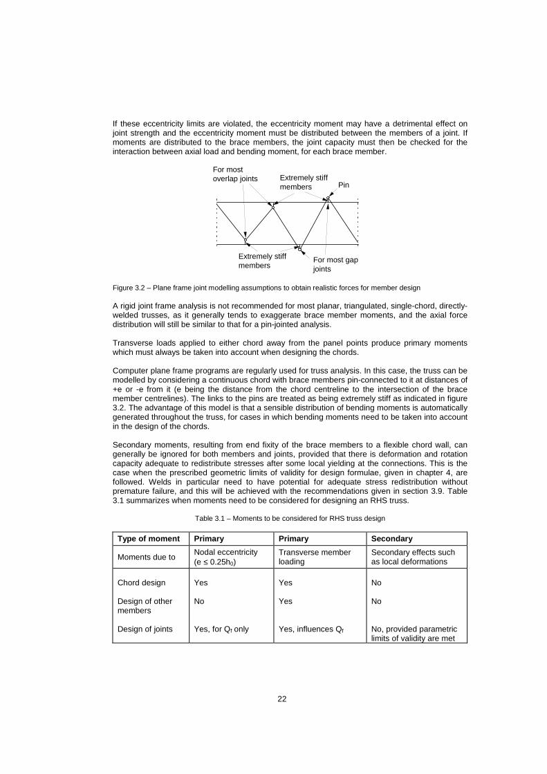
If these eccentricity limits are violated, the eccentricity moment may have a detrimental effect on joint strength and the eccentricity moment must be distributed between the members of a joint. If moments are distributed to the brace members, the joint capacity must then be checked for the interaction between axial load and bending moment, for each brace member.

For mostoverlap joints Extremely stiff

members Pin

Extremely stiffmembers

For most gapjoints

Figure 3.2 – Plane frame joint modelling assumptions to obtain realistic forces for member design A rigid joint frame analysis is not recommended for most planar, triangulated, single-chord, directly-welded trusses, as it generally tends to exaggerate brace member moments, and the axial force distribution will still be similar to that for a pin-jointed analysis. Transverse loads applied to either chord away from the panel points produce primary moments which must always be taken into account when designing the chords. Computer plane frame programs are regularly used for truss analysis. In this case, the truss can be modelled by considering a continuous chord with brace members pin-connected to it at distances of +e or -e from it (e being the distance from the chord centreline to the intersection of the brace member centrelines). The links to the pins are treated as being extremely stiff as indicated in figure 3.2. The advantage of this model is that a sensible distribution of bending moments is automatically generated throughout the truss, for cases in which bending moments need to be taken into account in the design of the chords. Secondary moments, resulting from end fixity of the brace members to a flexible chord wall, can generally be ignored for both members and joints, provided that there is deformation and rotation capacity adequate to redistribute stresses after some local yielding at the connections. This is the case when the prescribed geometric limits of validity for design formulae, given in chapter 4, are followed. Welds in particular need to have potential for adequate stress redistribution without premature failure, and this will be achieved with the recommendations given in section 3.9. Table 3.1 summarizes when moments need to be considered for designing an RHS truss.

Table 3.1 – Moments to be considered for RHS truss design

Type of moment Primary Primary Secondary

Moments due to Nodal eccentricity (e ≤ 0.25h0)

Transverse member loading

Secondary effects such as local deformations

Chord design Design of other members Design of joints

Yes No Yes, for Qf only

Yes Yes Yes, influences Qf

No No No, provided parametric limits of validity are met

23

Plastic design could be used to proportion the chords of a truss by considering them as continuous beams with pin supports from the brace members. In such a design, the plastically designed members must be plastic design sections and the welds must be sized to develop the capacity of the connected brace members. 3.3 Effective lengths for compression members To determine the effective length KL for a compression member in a truss, the effective length factor K can always be conservatively taken as 1.0. However, considerable end restraint is generally present for compression members in an RHS truss, and it has been shown that K is generally appreciably less than 1.0 (Mouty, 1981; Rondal et al., 1996). This restraint offered by members framing into a joint could disappear, or be greatly reduced, if all members were designed optimally for minimum mass, thereby achieving ultimate capacity simultaneously under static loading (Galambos, 1998). In practice, design for optimal or minimum mass will rarely coincide with minimum cost; the brace members are usually standardized to a few selected dimensions (perhaps even two) to minimize the number of section sizes for the truss. In the unlikely situation that all compression brace members are proportioned on the basis of a single load combination, and all reach their compressive resistances at approximately the same truss loading, an effective length factor of 1.0 is recommended. CIDECT has sponsored and coordinated extensive research work to specifically address the determination of effective lengths in hollow section trusses, resulting in reports from CIDECT Programmes 3E-3G and Monograph No. 4 (Mouty, 1981). A re-evaluation of all test results has been undertaken to produce recommendations for Eurocode 3. This has resulted in the following effective length recommendations. 3.3.1 Simplified rules For RHS chord members: In the plane of the truss: KL = 0.9 L where L is the distance between chord panel points 3.1 In the plane perpendicular to the truss: KL = 0.9 L where L is the distance between points of lateral support for the chord 3.2 For RHS or CHS brace members: In either plane: KL = 0.75 L where L is the panel point to panel point length of the member 3.3 These values of K are only valid for hollow section members which are connected around the full perimeter of the member, without cropping or flattening of the members. Compliance with the joint design requirements of chapter 4 will likely place even more restrictive control on the member dimensions. More detailed recommendations, resulting in lower K values are given in CIDECT Design Guide No. 2 (Rondal et al., 1996). 3.3.2 Long, laterally unsupported compression chor ds Long, laterally unsupported compression chords can exist in pedestrian bridges such as U-framed trusses and in roof trusses subjected to large wind uplift. The effective length of such laterally unsupported truss chords can be considerably less than the unsupported length. For example, the actual effective length of a bottom chord, loaded in compression by uplift, depends on the loading in the chord, the stiffness of the brace members, the torsional rigidity of the chords, the purlin to truss

24

joints and the bending stiffness of the purlins. The brace members act as local elastic supports at each panel point. When the stiffness of these elastic supports is known, the effective length of the compression chord can be calculated. A detailed method for effective length factor calculation has been given by CIDECT Monograph No. 4 (Mouty, 1981). 3.4 Truss deflections For the purpose of checking the serviceability condition of overall truss deflection under specified (unfactored) loads, an analysis with all members being pin-jointed will provide a conservative (over)estimate of truss deflections when all the joints are overlapped (Coutie et al., 1987; Philiastides, 1988). A better assumption for overlap conditions is to assume continuous chord members and pin-jointed brace members. However, for gap-connected trusses, a pin-jointed analysis still generally underestimates overall truss deflections, because of the flexibility of the joints. At the service load level, gap-connected RHS truss deflections may be underestimated by up to 12-15% (Czechowski et al., 1984; Coutie et al., 1987; Philiastides, 1988; Frater, 1991). Thus, a conservative approach for gap-connected RHS trusses is to estimate the maximum truss deflection by 1.15 times that calculated from a pin-jointed analysis. 3.5 General joint considerations It is essential that the designer has an appreciation of factors which make it possible for RHS members to be connected together at truss panel points without extensive (and expensive) reinforcement. Apparent economies from minimum-mass member selection will quickly vanish at the joints if a designer does not have knowledge of the critical considerations which influence joint efficiency. 1. Chords should generally have thick walls rather than thin walls. The stiffer walls resist loads from the brace members more effectively, and the joint resistance thereby increases as the width-to-thickness ratio decreases. For the compression chord, however, a large thin section is more efficient in providing buckling resistance, so for this member the final RHS wall slenderness will be a compromise between joint strength and buckling strength, and relatively stocky sections will usually be chosen. 2. Brace members should have thin walls rather than thick walls (except for the overlapped brace in overlap joints), as joint efficiency increases as the ratio of chord wall thickness to brace wall thickness increases. In addition, thin brace member walls will require smaller fillet welds for a pre-qualified connection (weld volume is proportional to t2). 3. Ideally, RHS brace members should have a smaller width than RHS chord members, as it is easier to weld to the flat surface of the chord section. 4. Gap joints (K and N) are preferred to overlap joints because the members are easier to prepare, fit and to weld. In good designs, a minimum gap g ≥ t1 + t2 should be provided such that the welds do not overlap each other. 5. When overlap joints are used, at least a quarter of the width (in the plane of the truss) of the overlapping member needs to be engaged in the overlap; i.e. q ≥ 0.25p in figure 1.1. However, q ≥ 0.5p is preferable. 6. An angle of less than 30° between a brace member and a chord creates serious welding difficulties at the heel location on the connecting face and is not covered by the scope of these recommendations (see section 3.9). However, angles less than 30° may be possible if the design is based on an angle of 30° and it is shown by the fabricator that a satisfactory weld can be made.

25

3.6 Truss design procedure In summary, the design of an RHS truss should be approached in the following way to obtain an efficient and economical structure. I. Determine the truss layout, span, depth, panel lengths, truss and lateral bracing by the usual methods, but keep the number of joints to a minimum. II. Determine loads at joints and on members; simplify these to equivalent loads at the panel points if performing manual analysis. Ill. Determine axial forces in all members by assuming that joints are either: (a) pinned and that all member centre lines are noding, or (b) that the chord is continuous with pin-connected braces. IV. Determine chord member sizes by considering axial loading, corrosion protection and RHS wall slenderness. (Usual width-to-thickness ratios b0/t0 are 15 to 25.) An effective length factor of K = 0.9 can be used for the design of the compression chord. Taking account of the standard mill lengths in design may reduce the end-to-end joints within chords. For large projects, it may be agreed that special lengths are delivered. Since the joint strength depends on the yield stress of the chord, the use of higher strength steel for chords (when available and practical) may offer economical possibilities. The delivery time of the required sections has to be checked. V. Determine brace member sizes based on axial loading, preferably with thicknesses smaller than the chord thickness. The effective length factor for the compression brace members can initially be assumed to be 0.75 (see section 3.3.1). VI. Standardize the brace members to a few selected dimensions (perhaps even two), to minimize the number of section sizes for the structure. Consider availability of all sections when making member selections. For aesthetic reasons, a constant outside member width may be preferred for all brace members, with wall thicknesses varying; but this will require special quality control procedures in the fabrication shop. VII. Layout the joints; from a fabrication point of view, try gap joints first. Check that the joint geometry and member dimensions satisfy the validity ranges for the dimensional parameters given in chapter 4, with particular attention to the eccentricity limit. Consider the fabrication procedure when deciding on a joint layout. VIII. If the joint resistances (efficiencies) are not adequate, modify the joint layout (for example, overlap rather than gap) or modify the brace or chord members as appropriate, and recheck the joint capacities. Generally, only a few joints will need checking. IX. Check the effect of primary moments on the design of the chords. For example, use the proper load positions (rather than equivalent panel point loading that may have been assumed if performing manual analysis); determine the bending moments in the chords by assuming either: (a) pinned joints everywhere or (b) continuous chords with pin-ended brace members. For the compression chord, also determine the bending moments produced by any noding eccentricities, by using either of the above analysis assumptions. Then check that the factored resistance of all chord members is still adequate, under the influence of both axial loads and total primary bending moments. X. Check truss deflections (see section 3.4) at the specified (unfactored) load level, using the proper load positions. XI. Design welds.

26

3.7 Arched trusses The joints of arched trusses can be designed in a similar way to those of straight chord trusses. If the arched chords are made by bending at the joint location only, as shown in figure 3.3(a), the chord members can also be treated in a similar way to those of straight chord trusses provided that the bending radius remains within the limits to avoid distortion of the cross section (Dutta et al., 1998; Dutta, 2002). If the arched chords are made by continuous bending, the chord members have a curved shape between the joint locations, as shown in figure 3.3(b). In this case, the curvature should be taken into account in the member design by treating the chord as a beam-column. (Moment = axial force x eccentricity.)

(a)

(b)

(c)

e

Figure 3.3 – Arched truss 3.8 Guidelines for earthquake design In seismic design, the joints should meet additional requirements with regard to overstrength, resulting in the members being critical. For sufficient rotation capacity, energy-dissipating members should meet at least the class 1 requirements of table 1.1. For detailed information, reference is given to CIDECT Design Guide No. 9 (Kurobane et al., 2004). 3.9 Design of welds Except for certain K and N joints with partially overlapped brace members (as noted below), a welded connection should be established around the entire perimeter of a brace member by means of a butt weld, a fillet weld, or a combination of the two. Fillet welds which are automatically prequalified for any brace member loads should be designed to give a resistance that is not less than the brace member capacity. According to Eurocode 3 (CEN, 2005b), this results in the following minimum throat thickness “a” for fillet welds around brace members, assuming matched electrodes and ISO steel grades (IIW, 2009): a ≥ 0.92 t, for S235 (fyi = 235 N/mm2) a ≥ 0.96 t, for S275 (fyi = 275 N/mm2) a ≥ 1.10 t, for S355 (fyi = 355 N/mm2) a ≥ 1.42 t, for S420 (fyi = 420 N/mm2) a ≥ 1.48 t, for S460 (fyi = 460 N/mm2) With overlapped K and N joints, welding of the toe of the overlapped member to the chord is particularly important for 100% overlap situations. For partial overlaps, the toe of the overlapped member need not be welded, providing the components, normal to the chord, of the brace member

27

forces do not differ by more than about 20%. The larger width brace member should be the “through member”. If both braces have the same width then the thicker brace should be the overlapped (through) brace and pass uninterrupted through to the chord. If both braces are of the same size (outside dimension and thickness), then the more heavily loaded brace member should be the “through member”. When the brace member force components normal to the chord member differ by more than 20%, the full circumference of the through brace should be welded to the chord. Generally, the weaker member (defined by wall thickness times yield strength) should be attached to the stronger member, regardless of the load type, and smaller members sit on larger members.

Figure 3.4 – Weld details It is more economical to use fillet welds than butt (groove) welds. However, the upper limit on throat or leg size for fillet welds will depend on the fabricator. Most welding specifications only allow fillet welding at the toe of a brace member if θi ≥ 60°. Because of the difficulty of welding at the heel of a brace member at low θ values, a lower limit for the applicability of the joint design rules given herein has been set at θi = 30°. Some recommended weld details (IIW, 2009) are illustrated in figure 3.4. If welds are proportioned on the basis of particular brace member loads, the designer must recognize that the entire length of the weld may not be effective, and the model for the weld resistance must be justified in terms of strength and deformation capacity. An effective length of RHS brace member welds in planar, gap K and N joints subjected to predominantly static axial load, is given by Frater and Packer (1990):

ii

i bθsin

h2length Effective += for θi ≥ 60° 3.4

ii

i b2θsin

h2length Effective += for θi ≤ 50° 3.5

For 50° < θi < 60°, a linear interpolation has been suggested ( AWS, 2008). For overlapped K and N joints, limited experimental research on joints with 50% overlap has shown that the entire overlapping brace member contact perimeter can be considered as effective (Frater and Packer, 1990). These recommendations for effective weld Iengths in RHS K and N joints satisfy the required safety levels for use in conjunction with both European and North American steelwork specifications (Frater and Packer, 1990). However it is recommended that the strength enhancement for transversely loaded fillet welds – allowed by some steel codes/specifications – not be used,

28

because the fillet weld is loaded by a force not in the plane of the weld group (AISC, 2005; Packer et al., 2009). Based on the weld effective Iengths for K and N joints, extrapolation has been postulated for RHS T, Y and X joints under predominantly static load (Packer and Wardenier, 1992):

i

i

θsinh2

length Effective = for θi ≥ 60° 3.6

ii

i bθsin

h2length Effective += for θi ≤ 50° 3.7

For 50° < θi < 60°, a linear interpolation is recommended.

Pavilion at Expo 92, Seville, Spain

29

4 Welded uniplanar truss joints between RHS chords and RHS or CHS brace (web) members

4.1 Joint classification

N1

t0 b0

h0

h1

b1 t1

θ1 = 90°

b1 h1

h0

b0

h2

t1 N1 g

-e

t0

N2 t2

b2

θ1 θ2

-e

θi t0 b0

h0

hi bi

ti

tj

hj

bj

Nj Ni θj = 90°

θ1 N1

N1

b0

h0

t0

t1

h1 b1

(a) T joint

(c) K gap joint (d) N overlap joint

(b) X joint

Figure 4.1 – Basic joint configurations i.e. T, X and K joints Figure 4.1 shows the basic types of joint configurations; i.e. T, X and K or N joints. The classification of hollow section truss-type joints as K (which includes N), Y (which includes T) or X joints is based on the method of force transfer in the joint, not on the physical appearance of the joint. Examples of such classification are shown in figure 4.2, and definitions follow. (a) When the normal component of a brace member force is equilibrated by beam shear (and bending) in the chord member, the joint is classified as a T joint when the brace is perpendicular to the chord, and a Y joint otherwise. (b) When the normal component of a brace member force is essentially equilibrated (within 20%) by the normal force component of another brace member (or members), on the same side of the joint, the joint is classified as a K joint. The relevant gap is between the primary brace members whose loads equilibrate. An N joint can be considered as a special type of K joint. (c) When the normal force component is transmitted through the chord member and is equilibrated by a brace member (or members) on the opposite side, the joint is classified as an X joint. (d) When a joint has brace members in more than one plane, the joint is classified as a multiplanar joint (see chapter 6).

30

gap

θ θ

N100%

KN

θ θ

1.2N100%

K

N

0.2N sinθ

within tolerancefor:

(a) (b)

θ

100%

K

N50% K50% X

+e0.5N sinθ

0.5N sinθ

θ

N100%

Y0

(c) (d)

θ θ

N100%

XN

2N sinθ

gap

θ θ

N 100%

K N100%

K

0

+e

(e) (f)

θ

N

100%

X

θ

N

(g) Figure 4.2 – Examples of hollow section joint classification

31

When brace members transmit part of their load as K joints and part of their load as T, Y, or X joints, the adequacy of each brace needs to be determined by linear interaction of the proportion of the brace load involved in each type of load transfer. One K joint, in figure 4.2(b), illustrates that the brace force components normal to the chord member may differ by as much as 20% and still be deemed to exhibit K joint behaviour. This is to accommodate slight variations in brace member forces along a typical truss, caused by a series of panel point loads. The N joint in figure 4.2(c), however, has a ratio of brace force components normal to the chord member of 2:1. In this case, that particular joint needs to be analysed as both a “pure” K joint (with balanced brace forces) and an X joint (because the remainder of the diagonal brace load is being transferred through the joint), as shown in figure 4.3. For the diagonal tension brace in that particular joint, one would need to check that:

1.0resistance joint X

0.5Nresistance jointK 0.5N ≤+

The three diagrams in figure 4.3 are each in equilibrium. If an additional chord “preload” force was applied to figure 4.3(a), on the left hand side, which would cause an equal and opposite additional chord force on the right hand side of the joint, then this “preload” would need to be added to either figure 4.3(b) or (c). It is recommended that this preload effect be added to the diagram which results in the more punitive outcome.

0.5N sinθ

0.5N sinθ

θ

N

N cosθ=

0.5N sinθ

θ

0.5N

0.5N cosθ0.5N sinθ

θ+

0.5N

0.5N cosθ

(a) (b) (c) Figure 4.3 – Checking of a K joint with imbalanced brace loads If the gap size in a gapped K (or N) joint (e.g. figure 4.2(a)) becomes large and exceeds the value permitted by the gap/eccentricity limit, then the “K joint” should also be checked as two independent Y joints. In X joints such as figure 4.2(e), where the braces are close together or overlapping, the combined “footprint” of the two braces can be taken as the loaded area on the chord member. In K joints such as figure 4.2(d), where a brace has very little or no loading, the joint can be treated as a Y joint, as shown. Some special uniplanar joints with braces on both sides of the chord where the brace forces act in various ways, are dealt with in table 4.4. 4.2 Failure modes The strength of RHS joints can, depending on the type of joint, geometric parameters and loading, be governed by various criteria. The majority of RHS truss joints have one compression brace member and one tension brace member welded to the chord as shown in figure 1.2. Experimental research on RHS welded truss

32

joints (for example Wardenier and Stark, 1978) has shown that different failure modes exist depending on the type of joint, loading conditions, and various geometric parameters. Failure modes for RHS joints have been described by Wardenier (1982) as illustrated in figure 4.4, and the design of welded RHS joints is thus based on these potential limit states. These failure modes are: Mode (a): Plastic failure of the chord face (one brace member pushes the face in, and the other

pulls it out) Mode (b): Punching shear failure of the chord face around a brace member (either compression or

tension) Mode (c): Rupture of the tension brace or its weld, due to an uneven load distribution (also termed

“local yielding of the brace”) Mode (d): Local buckling of the compression brace, due to an uneven load distribution (also

termed “local yielding of the brace”) Mode (e): Shear failure of the chord member in the gap region (for a gapped K joint) Mode (f): Chord side wall bearing or local buckling failure, under the compression brace Mode (g): Local buckling of the connecting chord face behind the heel of the tension brace. In addition to these failure modes, section 4.4 gives a detailed description of the typical failure modes found for K and N overlap joints. Failure in test specimens has also been observed to be a combination of more than one failure mode. It should be noted here that modes (c) and (d) are generally combined together under the term “local yielding of the brace” failures and are treated identically since the joint resistance in both cases is determined by the effective cross section of the critical brace member, with some brace member walls possibly being only partially effective. Plastic failure of the chord face (mode (a)) is the most common failure mode for gap joints with small to medium ratios of the brace member widths to the chord width β. For medium width ratios (β = 0.6 to 0.8), this mode generally occurs in combination with tearing in the chord (mode (b)) or the tension brace member (mode (c)) although the latter is only observed in joints with relatively thin-walled brace members. Mode (d), involving local buckling of the compression brace member, is the most common failure mode for overlap joints. Shear failure of the entire chord section (mode (e)) is observed in gap joints where the width (or diameter) of brace members is close to that of the chord (β ≈ 1.0), or where h0 < b0. Local buckling failure (modes (f) and (g)) occurs occasionally in RHS joints with high chord width (or depth) to thickness ratios (b0/t0 or h0/t0). Mode (g) is taken into account by considering the total normal stress in the chord connecting face, via the term n in the function Qf (see table 4.1). Wardenier (1982) concluded that in selected cases, just one or two governing modes can be used to predict joint resistance. Similar observations as above can be made for T, Y and X joints. Various formulae exist for joint failure modes analogous to those described above. Some have been derived theoretically, while others are primarily empirical. The general criterion for design is ultimate resistance, but the recommendations presented herein, and their limits of validity, have been set such that a limit state for deformation is not exceeded at specified (service) loads.

33

(a) Chord face plastification (b) Punching shear failure of the chord

(c) Uneven load distribution, in the tension brace (d) Uneven load distribution, in the compression

brace

(e) Shear yielding of the chord, in the gap (f) Chord side wall failure

(g) Local buckling of the chord face

Figure 4.4 – Failure modes for K and N type RHS truss joints 4.3 Joint resistance equations for T, Y, X and K ga p joints Recently, Sub-commission XV-E of the International Institute of Welding has reanalysed all joint resistance formulae. Based on rigorous examinations in combination with additional finite element (FE) studies, new design resistance functions have been established (IIW, 2009; Zhao et al., 2008).

34

For RHS joints, the additional analyses mainly concern the modification of the chord stress functions. The reanalyses also showed that for large tensile chord loads, a reduction of the joint resistance has to be taken into account (Wardenier et al., 2007a, 2007b). Further, as mentioned in section 1.1, the design equations for RHS K gap joints in the 1st edition of this Design Guide (Packer et al., 1992) are based on experiments undertaken in the 1970s (see e.g. Wardenier, 1982), prior to the introduction of a deformation limit of 0.03b0, and ultimate deformations may have exceeded this limit. Although these design formulae have proved to be satisfactory in practice, a modification is made to limit deformations and to extend the validity range. The new equation for K gap joints gives, compared to the previous equation, a modification in the γ effect and is a reasonable compromise between covering the N1(3%) data, extension of the validity range and backup by previous analyses (Packer and Haleem, 1981; Wardenier, 1982). The new limit states design recommendations for RHS T, Y, X and K gap joints are given in tables 4.1 and 4.2. For distinction from the formulae in the previous edition, which are incorporated in many national and international codes, a slightly different presentation is used. For example, for chord (face) plastification, the general resistance equation is presented as follows:

i

20 y0

f u*i

θsin

tf QQN = 4.1

The parameter Qu gives the influence function for the parameters β and γ, while the parameter Qf accounts for the influence of the chord stress on the joint capacity. In table 4.1 the total (normal) stress ratio, n, in the chord connecting face, due to axial load plus bending moment, is computed and its effect on joint resistance determined. It should be noted that the most punitive stress effect, Qf, in the chord on either side of the joint is to be used. The Qf functions are graphically presented in figures 4.5 to 4.7 for the individual effects of chord axial loading on T, Y, and X joints, chord moment loading on T, Y, and X joints, and chord axial loading on K gap joints. As shown in figures 4.5 and 4.6, the chord bending compression stress effect for T, Y and X joints is the same as that for chord axial compression loading. The range of validity of the formulae, given in table 4.1, is about the same as in the previous edition of this Design Guide, recorded in table A1a of Appendix A. However, as indicated in section 1.2.1, the validity range has been extended to steels with yield stresses up to fy = 460 N/mm2 (Liu and Wardenier, 2004). For yield stresses fy > 355 N/mm2, the joint resistance should be multiplied by a reduction factor of 0.9. Fleischer and Puthli (2008) investigated the potential expansion of the validity ranges for the K joint gap size and the chord cross section slenderness, and the potential consequences this might have. For the other criteria, the formulae are similar to those in the previous edition, although the presentation is slightly different. The effects of the differences on the joint resistance formulae given in the previous edition of this Design Guide, are presented in Appendix A. Table 4.2, restricted to square RHS or CHS braces and square RHS chords, is derived from the more general table 4.1 and uses more confined geometric parameters. As a result, T, Y, X and gap K and N joints with square RHS need only be examined for chord face failure, whereas those with rectangular RHS must be considered for nearly all failure modes. This approach has allowed the creation of useful graphical design charts which are later presented for joints between square RHS.

35

4.3.1 K and N gap joints From examination of the general limit states design recommendations, summarized in table 4.1 and those in table 4.2 for SHS, a number of observations can be made for K and N joints: - A common design criterion for all K and N gap joints is plastic failure of the chord face. The

constants in the resistance equations are derived from extensive experimental data, and the other terms reflect ultimate strength parameters such as plastic moment capacity of the chord face per

unit length ,4/tf 200y brace to chord width ratio β, chord wall slenderness 2γ, and the term Qf which

accounts for the influence of chord normal stress in the connecting face. - Tables 4.1 and 4.2 show that the resistance of a gap K or N joint with an RHS chord is largely

independent of the gap size (no gap size parameter). - In table 4.1, the check for chord shear in the gap of K and N joints involves dividing the chord

cross section into two portions. The first part is the shear area AV comprising the side walls plus part of the top flange, shown in figure 4.8, which can carry both shear and axial loads interactively. The contribution of the top flange increases with decreasing gap. The second part involves the remaining area A0-AV, which is effective in carrying axial forces only.

4.3.2 T, Y and X joints In the same way as an N joint is considered to be a particular case of the general K joint, the T joint is a particular case of the Y joint. The basic difference between the two types is that in T and Y joints, the component of load perpendicular to the chord is resisted by shear and bending in the chord, whereas for K or N joints, the normal component in one brace member is balanced primarily by the same component in the other brace. The limit states design recommendations for T, Y and X joints are summarized in table 4.1 (for rectangular chords) and table 4.2 (for square chords). Various observations can be made from the tables:

- Resistance equations in tables 4.1 and 4.2 for chord face plastification (with β ≤ 0.85), are based on a yield line mechanism in the RHS chord face. By limiting joint design capacity under factored loads to the joint yield load, one ensures that deformations will be acceptable at specified (service) load levels.

- For full width (β = 1.0) RHS T, Y and X joints, flexibility does not govern and resistance is based

on either the tension capacity or the compression instability of the chord side walls, for tension and compression brace members respectively.

- Compression loaded, full-width RHS X joints are differentiated from T or Y joints as their side

walls exhibit greater deformation than T joints. Accordingly, the value of fk in the resistance equation used for X joints is reduced by a factor 0.8sin θ1 compared to the value adopted for T or Y situations. In both instances, for 0.85 < β < 1.0, a linear interpolation between the resistance at β = 0.85 (where flexure of the chord face governs) and the resistance at β = 1.0 (where chord side wall failure governs) is recommended. Furthermore, if the angle θ1 becomes small (cos θ1 > h1/h0), shear failure of the chord can occur in X joints.

- All RHS T, Y and X joints with high brace width to chord width ratios (β ≥ 0.85) should also be

checked for local yielding of the brace and for punching shear of the chord face. For this range of width ratios, the brace member loads are largely carried by their side walls parallel to the chord while the walls transverse to the chords transfer relatively little load. The upper limit of β = 1 – 1/γ for checking punching shear is determined by the physical possibility of such a failure, when one considers that the shear has to take place between the outer limits of the brace width and the inner face of the chord wall.

36

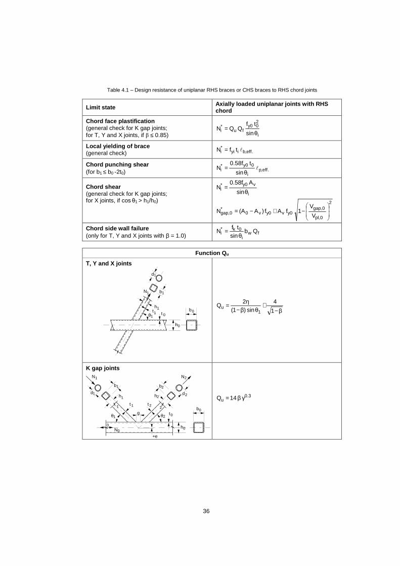
Table 4.1 – Design resistance of uniplanar RHS braces or CHS braces to RHS chord joints

Limit state Axially loaded uniplanar joints with RHS chord

Chord face plastification (general check for K gap joints; for T, Y and X joints, if β ≤ 0.85) i

20 y0

f u*i

θsin

tfQQN =

Local yielding of brace (general check) .eff,b i yi

*i tfN l=

Chord punching shear (for b1 ≤ b0 -2t0) .eff,p

i

0 y0*i

θsin

t0.58fN l=

Chord shear (general check for K gap joints; for X joints, if cos θ1 > h1/h0)

i

v y0*i

θsin

A0.58fN =

2

pl,0

gap,0 y0 vy0 v0

*gap,0 V

V1fAf)A(AN

−+−=

Chord side wall failure (only for T, Y and X joints with β = 1.0) fw

i

0 k*i Qb

θsintf

N =

Function Q u

T, Y and X joints

t 0 t 1

d 1

h 1

b 1

h 0

b 0

N 1

θ 1

β−+

β−η=

1

4θnsi )1(

2Q

1 u

K gap joints

g

d 1

θ 1 θ 2 t 0

t 2 2 1

+e

0

h 1

b 1

d 2h 2

b 2

h 0

b 0t 1

N 0

N 1 N 2

3.0u 14Q γβ=

37

Table 4.1 – Design resistance of uniplanar RHS braces or CHS braces to RHS chord joints (continued)

Function Q f

1Cf )n(1Q −= with

0,pl

0

0,pl

0

MM

NN

n += in connecting face

Chord compression stress (n < 0) Chord tension stress (n ≥≥≥≥ 0)

T, Y and X joints C1 = 0.6 - 0.5β C1 = 0.10

K gap joints C1 = 0.5 - 0.5β but ≥ 0.10

l b,eff. and l p,eff. l b,eff. l p,eff.

T, Y and X joints )4t2b(2h 1e1.eff,b −+=l

+= pe,

1

1.eff,p 2b

θsin2h

l

K gap joints )4tbb(2h ieii.eff,b −++=l

++= pe,i

i

i.eff,p bb

θsin2h

l

iiiyi

0 0y

00e b but b

tf

tf

/tb10

b ≤

= ii

00p,e b but b

/tb10

b ≤

=

Av and V pl,0 v y0pl,0 A0.58fV =

T, Y and X joints 00v t2hA =

K gap joints 0000v tb t2hA α+=

RHS braces CHS braces

)t3/()g4(1

120

2+=α 0=α

bw ββββ = 1.0 0.85 < ββββ < 1.0

T, Y and X joints

+= 0

1

1w 10t

θsin2h

b Use linear interpolation between the resistance for chord face plastification at β = 0.85 and the resistance for chord side wall failure at β = 1.0.

K gap joints N/A

fk Brace tension Brace compression

0yk ff =

T and Y joints X joints

0yk ff χ= 1 y0k θsinf8.0f χ=

where χ = reduction factor for column buckling according to e.g. Eurocode 3 (CEN, 2005a) using the relevant buckling curve and a slenderness

1 0

0

θsin1

2th

3.46

−=λ

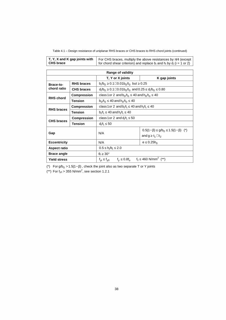
38

Table 4.1 – Design resistance of uniplanar RHS braces or CHS braces to RHS chord joints (continued)

T, Y, X and K gap joints with CHS brace

For CHS braces, multiply the above resistances by π/4 (except for chord shear criterion) and replace bi and hi by di (i = 1 or 2)

Range of validity

T, Y or X joints K gap joints

Brace-to-chord ratio

RHS braces 0.25but /t0.01b0.1/bb 000i ≥+≥

CHS braces 000i /t0.01b0.1/bd +≥ and 80.0/bd 0.25 0i ≤≤

RHS chord Compression 2 or 1 class 40/th and 40/tb and 0000 ≤≤

Tension 40/th and 40/tb 0000 ≤≤

RHS braces Compression 2 or 1 class 40/th and 40 /tb and iiii ≤≤

Tension 40/th and 40/tb iiii ≤≤

CHS braces Compression 2 or 1 class 50/td and ii ≤

Tension 50/td ii ≤

Gap N/A )1(5.1g/b)1(5.0 0 β−≤≤β− (*)

and 21 ttg +≥

Eccentricity N/A 0h25.0e ≤

Aspect ratio 0.2/bh5.0 ii ≤≤

Brace angle θi ≥ 30°

Yield stress y0yi ff ≤ uy f8.0f ≤ fy ≤ 460 N/mm2 (**)

(*) For )1(5.1g/b0 β−> , check the joint also as two separate T or Y joints

(**) For fy0 > 355 N/mm2, see section 1.2.1

39

Table 4.2 – Design resistance of uniplanar SHS or CHS braces to SHS chord joints

Limit state Axially loaded uniplanar joints with SHS chord

Chord face plastification i

20 y0

f u*i

θsin

tfQQN =

Function Q u

T, Y and X joints

t 0 t 1

d 1

h 1

b 1

h 0

b 0

N 1

θ 1

β−+

θβ−η=

1

4sin)1(

2Q

1u

K gap joints

g

d 1

θ 1 θ 2 t 0

t 2 2 1

+e

0

h 1

b 1

d 2h 2

b 2

h 0

b 0t 1

N 0

N 1 N 2

3.0u 14Q γβ=

Function Q f Same as in table 4.1

T, Y, X and K gap joints with CHS brace For CHS braces, multiply the above resistances by π/4 and replace bi by di (i = 1 or 2)

Range of validity

General Same as in table 4.1 with additional limits given below

SHS braces T, Y and X joints 85.0/bb 01 ≤

K gap joints 3.1))/(2bb(b6.0 i21 ≤+≤ 15/tb 00 ≥

CHS braces K gap joints 3.1))/(2dd(d6.0 i21 ≤+≤ 15/tb 00 ≥

40

X and T joints: chord axial stress functions T joints: chord bending stress func tion

0

0.1

0.2

0.3

0.4

0.50.6

0.7

0.8

0.9

1

-1 -0.8 -0.6 -0.4 -0.2 0 0.2 0.4 0.6 0.8 1n

Qf

β=0.4

β=0.6

β=0.8

β=1.0

Figure 4.5 – Chord axial stress functions Qf for T and X joints and chord bending stress function Qf for T joints

X joints: chord bending stress function

0

0.1

0.2

0.3

0.4

0.5

0.6

0.7

0.8

0.9

1

-1 -0.8 -0.6 -0.4 -0.2 0 0.2 0.4 0.6 0.8 1n

Qf

β=0.4

β=0.6

β=0.8

β=1.0

Figure 4.6 – Chord bending stress function Qf for X joints

K gap joints: chord axial stress functions

0.0

0.1

0.2

0.3

0.4

0.50.6

0.7

0.8

0.9

1.0

-1 -0.8 -0.6 -0.4 -0.2 0 0.2 0.4 0.6 0.8 1n

Qf

β=0.25

β=0.4

β=0.6

β=0.8−1.0

Figure 4.7 – Chord axial stress function Qf for K gap joints

41

Figure 4.8 – Shear area AV of the chord in the gap region of an RHS K or N joint 4.4 K and N overlap joints For overlap joints the same approach is adopted for all types of overlap joints, regardless of whether CHS or RHS braces are used in combination with a CHS, RHS or open section chord (Chen et al., 2005; Liu et al., 2005; Qian et al., 2007; Wardenier, 2007). Only the effective width factors depend on the type of section. The resistance of overlap joints between hollow sections with 25% ≤ Ov ≤ 100% overlap is based on the following criteria:

(1) Local yielding of the overlapping brace. (2) Local chord member yielding at the joint location, based on interaction between axial load and

bending moment. (3) Shear of the connection between the brace(s) and the chord. Figure 4.9 shows the overlap joint configuration with the cross sections to be examined for these criteria. For K and N overlap joints, the subscript i is used to denote the overlapping brace member, while the subscript j refers to the overlapped brace member.

Figure 4.9 – Overlap joint configuration with cross sections to be checked

t0

N0p

hj bj

tj

b0

h0

bi hi

ti

N0

θj θi

Ni Nj

(2) (2)

(3)

(1)

42

In the previous edition of this Design Guide (Packer et al., 1992), only the criterion for local yielding of the overlapping brace was given, whereas the chord member had to be checked for the combination of chord axial force and bending moment due to eccentricity. Since this last check was sometimes overlooked by the designers, it is now explicitly included in the design checks. Furthermore, in the case of large overlaps or for hi < bi and/or hj < bj, the shear force needs to be limited in order to avoid an excessively large concentrated shear at the brace-to-chord face connection. Although no fracture has been observed in previous tests, but only shear deformation, it was found that the criterion for this failure mode can be based on the ultimate shear capacity of the effective area of the connected braces. Table 4.3 presents the resistances for K overlap joints starting with 25% overlap, which is the minimum value to ensure overlap behaviour. The resistance increases linearly with overlap from 25% to 50%, is constant from 50% up to 100% and reaches a higher level at 100%. Figure 4.10 illustrates the physical interpretation of the expressions for the effective width given in table 4.1 for gap joints and in table 4.3 for overlap joints, whereas figure 4.11 shows this for the brace shear criterion. Local yielding of the overlapping brace (criterion 1) should always be verified, although shear between the braces and the chord (criterion 3) may become critical for larger overlaps, i.e. larger than 60% or 80%, depending on whether or not the hidden toe location of the overlapped brace is welded to the chord. The check for local chord member yielding (criterion 2) is, in principle, a member check and may become critical for larger overlaps and/or larger β ratios. For 100% overlap joints, similar criteria have to be verified. However, for such joints, shear of the overlapping brace or chord member yielding will generally be the governing criterion (Chen et al., 2005). Although an overlap can be assumed to be 100%, in general, the overlap will be slightly larger to allow proper welding of the overlapping brace to the overlapped brace. Joints with overlaps between 0% and 25% should be avoided because for such joints, the stiffness of the connection between the overlapping brace and the overlapped brace is much larger than that of the overlapping brace to chord connection, which may lead to premature cracking and lower capacities (Wardenier, 2007).

43

Figure 4.10 – Physical interpretation of the effective width terms for gap and overlap joints

hj bj

tj ti

hi bi

θj θi

0.5bej 0.5bei

hj/sinθj 0.5hi/sinθi

ti tj

hj bj

tj ti

hi bi

θj θi

0.5bej bj

hj/sinθj

tj

Figure 4.11 – Physical interpretation of the effective width terms for brace shear in overlap joints

0.5be,p

0.5be,p bi

0.5be,ov

0.5be,ov

bi

0.5be 0.5be

bi

0.5bei

0.5bei bi

(a) gap joints

(b) overlap joints

44

Table 4.3 – Design resistance of uniplanar overlap joints with RHS braces or CHS braces to RHS chord

Limit state Axially loaded overlap joints

Local yielding of overlapping brace .eff,b i yi*i tfN l=

Local chord member yielding 0.1MM

NN

0,pl

0

0,pl

0 ≤+

Brace shear (*) (for Ovlimit < Ov ≤ 100%)

*sj ji i NθcosNθcosN ≤+ (see table next page)

(*) Ovlimit = 60% if hidden seam of the overlapped brace is not welded Ovlimit = 80% if hidden seam of the overlapped brace is welded

.eff,bl

RHS braces CHS braces

25% ≤≤≤≤ Ov < 50% iove,eii.eff,b 4tbb)2h50Ov

( −++=l )t4ddd2(

4 iov,eeii.eff,b −++π=l

50% ≤≤≤≤ Ov < 100% iov,eeii.eff,b t4bbh2 −++=l

Ov = 100% iov,eii.eff,b t4bbh2 −++=l )t4d2d2(4 iov,ei.eff,b −+π=l

General note The efficiency (i.e. design resistance divided by the yield load) of the overlapped brace j shall not exceed that of the overlapping brace i

Range of validity

General

25.0/bb and /bb 0j0i ≥

25.0/bd and /bd 0j0i ≥

75.0/bb ji ≥

75.0/dd ji ≥

0ji tt and t ≤

ji tt ≤

θi and θj ≥ 30° Ov ≥ 25% y0yjyi ff and f ≤ uy f8.0f ≤

2y N/mm 460f ≤ (**)

RHS chord

Compression class 1 or 2 40/th and 40/tb and 0000 ≤≤ Tension 40/th and 40/tb 0000 ≤≤

Aspect ratio 0.2/bh5.0 00 ≤≤

RHS braces

Compression class 1 or 2 40/th and 40/tb and 1111 ≤≤

Tension 40/th and 40/tb 2222 ≤≤

Aspect ratio 0.2/bh5.0 and 0.2/bh5.0 jjii ≤≤≤≤

CHS braces Compression class 1 or 2 50/td and 11 ≤

Tension 50/td 22 ≤

(**) For fy0 > 355 N/mm2, see section 1.2.1

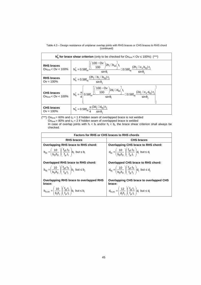
45

Table 4.3 – Design resistance of uniplanar overlap joints with RHS braces or CHS braces to RHS chord (continued)

*sN for brace shear criterion (only to be checked for Ovlimit < Ov ≤ 100%) (***)

RHS braces Ovlimit < Ov < 100%

j

jej sjuj

i

ieii

ui*s

θsin

t )bch2(f58.0

θsin

t bh2 100

Ov100

f58.0N+

+

+

−

=

RHS braces Ov = 100% j

jejjjuj

*s

θnsi

t )bbh2(f58.0N

++=

CHS braces Ovlimit < Ov < 100%

++

+

−π=

θsin

t )dcd2(f58.0

θsin

t dd2 100

Ov100

f58.04

Nj

jej sjuj

i

ieii

ui*s

CHS braces Ov = 100% j

jejjuj

*s

θsin

t )dd3(

4f58.0N

+π=

(***) Ovlimit = 60% and cs = 1 if hidden seam of overlapped brace is not welded Ovlimit = 80% and cs = 2 if hidden seam of overlapped brace is welded

In case of overlap joints with hi < bi and/or hj < bj, the brace shear criterion shall always be checked.

Factors for RHS or CHS braces to RHS chords

RHS braces CHS braces

Overlapping RHS brace to RHS chord:

iii yi

0 y0

00ei b but b

tf

tf

/tb10

b ≤

=

Overlapped RHS brace to RHS chord:

jjj yj

0 y0

00ej bbut b

tf

tf

/tb10

b ≤

=

Overlapping RHS brace to overlapped RHS brace:

iii yi

j yj

jjove, b but b

tf

tf

/tb10

b ≤

=

Overlapping CHS brace to RHS chord:

iii yi

0 y0

00ei d but d

tf

tf

/tb10

d ≤

=

Overlapped CHS brace to RHS chord:

jjj yj

0 y0

00ej dbut d

tf

tf

/tb10

d ≤

=

Overlapping CHS brace to overlapped CHS brace:

iii yi

j yj

jjove, dbut d

tf

tf

/td12

d ≤

=

46

4.5 Special types of joints In tubular structures, various joint configurations exist which have not been discussed in the previous chapters. However, the resistance of several types of joints can be directly related to the basic types presented in tables 4.1 and 4.2. Table 4.4 shows some special types of RHS uniplanar joints with braces directly welded to the chord.

Table 4.4 – Special types of uniplanar joints

Type of joint Relationship to the formulae of table s 4.1 and 4.2

*11 N N ≤

joint X from N with *1

i *i2 21 1 θsinN θsinNθsinN ≤+

joint X from 2) or 1(i N with *i =

2 *21 *

1i *i θsinN and θsinN of larger the is θsinN where

)2 or 1(i N N *ii =≤

force chord actual the withbut joint,K from )2 or 1(i N with *i =

)2 or 1(i N N *ii =≤

jointK from )2 or 1(i N with *i =

Note: Check cross section 1-1 for shear failure in the gap:

vy00,plgap,0 A0.58fVV =≤

2

0,pl

0,gap y0 vy0 v0

*0,gap0,gap V

V1fAf)A(ANN

−+−=≤

N1 N1 θ1 θ1

N2

N1

N1

N2

θ2 θ1

1

1

N2

N2

N1

N1

θ2 θ1

1

1

N2

N1

N1

N2

θ2 θ1

47

4.6 Graphical design charts with examples The joint design strength for joints with square hollow section members, as given in table 4.2, may be expressed in terms of the efficiency of the connected braces; i.e. the joint design resistance for

axially loaded joints *iN may be divided by the yield load Ai fyi of the connected brace. This results in

an efficiency formula of the following type:

i

f

i yi

0 y0e

yi i

*i

θsinQ

tf

tf C

fAN = 4.2

For each type of joint, the efficiency parameter Ce is given in the diagrams in tables 4.5 to 4.9. In general, Ce is a function of the width ratio β and the chord width-to-thickness ratio 2γ.

In the case of 21 bb ≠ for K joints, equation 4.2 has to be multiplied by i

21

2bbb +

, where bi is the

width of the brace considered. The value of the parameter Ce in equation 4.2 gives the joint efficiency for the brace of a joint with a chord stress effect Qf = 1.0, a brace angle θi = 90° and the same wall thickness and design yield stress for chord and brace. Except for overlapped K joints, the efficiencies given in the charts are termed CT, CX, or CK depending on the type of joint. Hence, these latter efficiencies need to be multiplied by the following three factors (see equation 4.2) to obtain the final joint efficiency in each case:

- The first factor, correcting for differing strengths between the chord and the brace member, is (fy0

t0)/(fyi ti). In general, this term is reduced to t0/ti, because the same grade of steel would normally be used throughout.

- The second factor, adjusting for the angle between the brace member and the chord, is 1/sin θi for square RHS T, Y, X and gap K joints. One should note that such an angle function is not considered for square RHS overlap joints because the efficiencies of these joints are based on the criterion for local yielding of the overlapping brace.

- The third factor, correcting for the influence of chord longitudinal stresses on the joint efficiency, is Qf. For RHS, Qf is defined in table 4.1 and plotted in figures 4.5 to 4.7. This function Qf is not included for overlap joints because for these joints, the strength function is based on the criterion for local yielding of the overlapping brace.

Simplifying assumptions and narrower validity parameters were sometimes necessary to simplify the presentation of the charts. Still, use of the design charts for T and X joints with θ1 = 90° and K joints in general, produces results close to the actual formulae. For Y and X joints with β ≤ 0.85, the results obtained with the design charts can be very conservative for θ1 < 90°. On the other hand, for Y and X joints with β > 0.85 subjected to brace compression, the design charts may give unconservative predictions for θ1 < 90°. Furthermore, it should be considered that the design charts have been based on a brace cross sectional area of 0.96(4b1t1). Hence, for sections with relatively large corner radii and/or stocky members, the graphs may give too optimistic results. In those cases it is recommended to reduce the calculated efficiency by about 10%. From the efficiency equation, it is evident that the yield stress and thickness ratio between the chord and brace is extremely important for an efficient material use of the brace. Furthermore, decreasing the angle θi increases the efficiency.

48

The efficiency formula shows directly that the following measures are favourable for the joint efficiency:

- brace wall thickness as small as possible (ti < t0), but such that the limits for local buckling are satisfied

- higher strength steel for chords than for braces (fy0 > fyi) - angle θi << 90°; hence, prefer K joints to N joints Three charts are presented for T, Y and X joints (tables 4.5 to 4.7). The first graph applies to each of the three joint types when the braces are loaded in tension; the second applies to T and Y joints when the braces are loaded in compression; the third to X joints with the braces loaded in compression. In addition to the failure mode listed in table 4.2 (chord face plastification for joints with β ≤ 0.85), the first three design charts also include chord side wall failure (for joints with β > 0.85). The three charts are identical for β values up to 0.85. However, when β exceeds 0.85, the behaviour of the chord side walls is different for the three situations, resulting in three separate charts. The graphs further show linear interpolations between the calculated resistances at β = 0.85 and β = 1.0. For gap K and N joints, the efficiency chart is given in table 4.8, which is slightly different from the graphs used for T, Y and X joints. For gap K joints, the efficiency CK is plotted as a function of 2γ

instead of β. Furthermore, for K gap joints, the correction with i

21

b2bb +

for 21 bb ≠ should be

included, where bi represents the width of the brace considered. Observation of the design resistances for joints with CHS braces shows that the efficiency for these joints can be directly obtained from the design graphs for square braces by using di instead of bi. The design resistance of joints with CHS braces is π/4 times that of RHS braces, which is about the ratio between the cross sectional areas of the braces for di = bi and the same ti. The range of overlap for SHS K and N joints, given in table 4.9, is from 50% to Ovlimit rather than for Ov ≥ 25% as presented in table 4.3. This avoids the more complex lower range where the resistance varies with the amount of overlap. However, above Ovlimit, which is 60 or 80%, the brace shear criterion has to be checked separately.

49

Table 4.5 – Efficiency design chart for SHS T, Y and X joints with brace(s) in tension

SHS T, Y and X joints with brace(s) in tension

Symbols Geometric range of validity

0

1

bb

β = 0

0

tb

2 =γ

t 0 t 1

d 1

h 1

b 1

h 0

b 0

N 1

θ 1

0.25 ≤ β ≤ 1.0 and β ≥ 0.1+0.02γ

compression chord: class 1 or 2 and 2γ ≤ 40 tension chord: 2γ ≤ 40

compression brace: class 1 or 2 and b1/t1 ≤ 40 tension brace: b1/t1 ≤ 40

θ1 ≥ 30° and cos θ1 ≤ h1/h0

Note: Use of the design chart results in conservative estimates for θ1 < 90°

Design chart

Efficiency T, Y and X joints in tension

0.0

0.1

0.2

0.3

0.4

0.5

0.6

0.7

0.8

0.9

1.0

0 0.1 0.2 0.3 0.4 0.5 0.6 0.7 0.8 0.9 1ββββ

CX o

r C

T

2γ=10

2γ=15

2γ=20

2γ=30

2γ=40

1

f

1 1y

0 0yT

1y1

*1

sinQ

tf

tfC

f AN

θ=

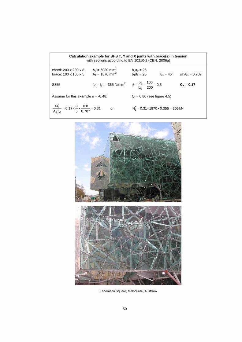
50

Calculation example for SHS T, Y and X joints with brace(s) in tension with sections according to EN 10210-2 (CEN, 2006a)

chord: 200 x 200 x 8 A0 = 6080 mm2 b0/t0 = 25 brace: 100 x 100 x 5 A1 = 1870 mm2 b1/t1 = 20 θ1 = 45° sin θ1 = 0.707

S355 fy0 = fy1 = 355 N/mm2 5.0200100

bb

0

1 ===β CX = 0.17

Assume for this example n = -0.48: Qf = 0.80 (see figure 4.5)

0.31 707.08.0

58

0.17fA

N

y1 1

*1 =××= or kN 206355.0187031.0N*

1 =××=

Federation Square, Melbourne, Australia

51

Table 4.6 – Efficiency design chart for SHS T and Y joints with brace in compression

SHS T and Y joints with brace in compression

Symbols Geometric range of validity

0

1

bb

β = 0

0

tb

2 =γ

t 0 t 1

d 1

h 1

b 1

h 0

b 0

N 1

θ 1

0.25 ≤ β ≤ 1.0 and β ≥ 0.1+0.02γ

compression chord: class 1 or 2 and 2γ ≤ 40 tension chord: 2γ ≤ 40

compression brace: class 1 or 2 and b1/t1 ≤ 40 tension brace: b1/t1 ≤ 40

θ1 ≥ 30°

Notes: - Use of the design chart results in unconser-

vative estimates for β > 0.85 with θ1 < 90° - For β > 0.85, diagram based on S355

Design chart

Efficiency T and Y joints in compression

0.0

0.1

0.2

0.3

0.4

0.5

0.6

0.7

0.8

0.9

1.0

0 0.1 0.2 0.3 0.4 0.5 0.6 0.7 0.8 0.9 1ββββ

CT

2γ=10

2γ=15

2γ=20

2γ=30

2γ=40

1

f

1 1y

0 0yT

1y1

*1

sinQ

tf

tfC

f AN

θ=

52

Calculation example for SHS T and Y joints with bra ce in compression with sections according to EN 10210-2 (CEN, 2006a)

chord: 100 x 100 x 8 A0 = 2880 mm2 b0/t0 = 12.5 brace: 100 x 100 x 5 A1 = 1870 mm2 b1/t1 = 20 θ1 = 90° sin θ1 = 1.0

S355 fy0 = fy1 = 355 N/mm 0.1100100

bb

β0

1 === CT = 0.68

Assume for this example n = -0.60 in bending: Qf = 0.91 (see figure 4.5)

0.99 91.058

0.68fA

N

y1 1

*1 =××= or kN 657355.0187099.0N*

1 =××=

RHS lattice girder

53

Table 4.7 – Efficiency design chart for SHS X joints with braces in compression

SHS X joints with braces in compression

Symbols Geometric range of validity

0

1

bb

β = 0

0

tb

2 =γ

t 0 t 1

d 1

h 1

b 1

h 0

b 0

N 1

θ 1

N 1

0.25 ≤ β ≤ 1.0 and β ≥ 0.1+0.02γ

compression chord: class 1 or 2 and 2γ ≤ 40 tension chord: 2γ ≤ 40

compression brace: class 1 or 2 and b1/t1 ≤ 40 tension brace: b1/t1 ≤ 40

θ1 ≥ 30° and cos θ1 ≤ h1/h0

Notes: - Use of the design chart results in unconser-

vative estimates for β > 0.85 with θ1 < 90° - For β > 0.85, diagram is based on S355

Design chart

Efficiency X joints in compression

only for θθθθ1 = 90o and f y = 355N/mm 2

0.0

0.1

0.2

0.3

0.4

0.5

0.6

0.7

0.8

0.9

1.0

0 0.1 0.2 0.3 0.4 0.5 0.6 0.7 0.8 0.9 1ββββ

CX

2γ=10

2γ=15

2γ=20

2γ=30

2γ=40

1

f

11y

0 0yX

1y 1

*1

sinQ

t f

tfC

fAN

θ=

54

Calculation example for SHS X joints with braces in compression with sections according to EN 10210-2 (CEN, 2006a)

chord: 150 x 150 x 10 A0 = 5490 mm2 b0/t0 = 15 brace: 120 x 120 x 5 A1 = 2270 mm2 b1/t1 = 24 θ1 = 90° sin θ1 = 1.0

S355 fy0 = fy1 = 355 N/mm2 8.0150120

bb

β0

1 === CX = 0.37

Assume for this example n = +0.60 in tension: Qf = 0.91 (see figure 4.5)

0.67 91.05

10 0.37

fAN

y1 1

*1 =××= or kN 540355.0227067.0N*

1 =××=

Pedestrian “Pony Truss” bridge

55

Table 4.8 – Efficiency design charts for SHS K and N gap joints

SHS K and N gap joints

Symbols Geometric range of validity

0

21

2bbb

β+=

0

0

tb

2 =γ

g

d 1

θ 1 θ 2 t 0

t 2 2 1

+e

0

h 1

b 1

d 2h 2

b 2

h 0

b 0t 1

N 0

N 1 N 2

0.25 ≤ β ≤ 1.0 and β ≥ 0.1+0.02γ compression chord: class 1 or 2 and 15 ≤ 2γ ≤ 40 tension chord: 15 ≤ 2γ ≤ 40

compression brace: class 1 or 2 and b1/t1 ≤ 40 tension brace: b2/t2 ≤ 40

3.1b2bb

6.0i

21 ≤+≤

0.5(1-β) ≤ g/b0 ≤ 1.5(1-β) and 21 ttg +≥

θi ≥ 30° 25.0he

0≤

Design chart

Efficiency K gap joints

0.0

0.1

0.2

0.3

0.4

0.5

0.6

0.7

0.8

0.9

1.0

15 20 25 30 35 402γ2γ2γ2γ

CK

i

21

1

f

1 1y

0 0yK

1y 1

*1

b2bb

sinQ

tf

tfC

fAN +

θ=

56

Calculation example for SHS K and N gap joints with sections according to EN 10210-2 (CEN, 2006a)

chord : 200 x 200 x 10 A0 = 7490 mm2 b0/t0 = 20 fy0 = fy1 = fy2 = 355 N/mm2 brace 1: 140 x 140 x 5 A1 = 2670 mm2 b1/t1 = 28 e = 0 mm brace 2: 120 x 120 x 5 A2 = 2270 mm2 b2/t2 = 24 g = 36 mm θ1 = θ2 = 40° sin θ1 = sin θ2 = 0.643

2010200

tb

20

0 ===γ 65.02002120140

b2bb

β0

21 =×

+=+=

Assume n = -0.8: Qf = 0.75 (see figure 4.7)

Thus: CK = 0.36 2 brace for 1.08 and 1, brace for 0.932b

bb with

i

21 =+

0.780.930.6430.75

510

0.36fA

N

y1 1

*1 =×××= 0.911.08

0.6430.75

510

0.36fA

N

y2 2

*2 =×××=

kN 739355.0267078.0N*1 =××= kN 733 355.0227091.0N*

2 =××=

Rack structure, for automated retrieval of pallets

57

Table 4.9 – Efficiency design chart for SHS K and N overlap joints (for 50% ≤ Ov ≤ Ovlimit = 60% or 80%)

SHS K and N overlap joints

Symbols Geometric range of validity

0

0

tb

2 =γ %100pq

Ov ×=

brace i = overlapping member brace j = overlapped member

0.25b

b and

b

b

0

j

0

i ≥ 0.75bb

j

i ≥ 1.0tt

j

i ≤

compression chord: class 1 or 2 and 2γ ≤ 40 tension chord: 2γ ≤ 40 compression brace: class 1 or 2 and b1/t1 ≤ 40 tension brace: b2/t2 ≤ 40 θi and θj ≥ 30° 50% ≤ Ov ≤ Ovlimit

Design chart

d i

d 0 θ i θ j t 0

t j j i

-e 0

h i

b i

d jh j

b j

h 0

b 0

t i

N i N j

N 0

p

q

eff= 0.5+0.25b ei/bi+0.25be,ov /bi

0.00

0.05

0.10

0.15

0.20

0.25

0.30

10 15 20 25 30 35 40

b0/t0 or b j /t j

0.25

bei/b

i or

0.25

be,

ov/b

i

fy.t ratio = 1.0

fy.t ratio = 1.5

fy.t ratio = 2.0

fy.t ratio = 2.5

fy.t ratio = 3.0

fy.t ratio = 1.0

fy.t ratio = 1.5

fy.t ratio = 2.0

fy.t ratio = 2.5

fy.t ratio = 3.0

58

Calculation example for SHS K and N overlap joints with sections according to EN 10210-2 (CEN, 2006a)

chord : 200 x 200 x 8 A0 = 6080 mm2 b0/t0= 25 fy0 = fyi = fyj = 355 N/mm2 brace i : 140 x 140 x 4 Ai = 2130 mm2 bi/ti = 35 (tension) Ov = 50% brace j : 150 x 150 x 5 Aj = 2870 mm2 bj/tj = 30 (compression) For Ov = 50%, besides member checks, only local yielding of the overlapping brace needs to be checked:

0.248

tf

tf

i yi

0 y0 == with b0/t0 = 25: 0.25bei/bi = 0.20

1.2545

tf

tf

i yi

j yj == with bj/tj = 30: 0.25be,ov/bi = 0.10

Hence, the brace efficiency for both braces is: Eff. = 0.50 + 0.25bei/bi + 0.25be,ov/bi = 0.50 + 0.20 + 0.10 = 0.80

kN 605355.021308.0N*i =××= kN 815355.028708.0N*

j =××=

Truss with 100% overlapped joint

59

5 Welded RHS-to-RHS joints under moment loading 5.1 Vierendeel trusses and joints 5.1.1 Introduction to Vierendeel trusses Arthur Vierendeel first proposed Vierendeel trusses in 1896. They are comprised of brace members connected to chord members usually at 90° angles (see figure 5.1).

Figure 5.1 – Application of RHS Vierendeel trusses in the foyer of a building The typical design premise with Vierendeel trusses has been to assume full joint rigidity, but this is rarely the case with RHS to RHS Vierendeel joints. Unlike triangulated Warren or Pratt trusses, in which the joints approximately behave as a pinned joint at their ultimate limit state and cause the brace members to be loaded by predominantly axial forces, Vierendeel joints have brace members subjected to substantial bending moments as well as axial and shear forces. Until recently, most of the testing performed on Vierendeel joints has been on isolated joint specimens as shown in figure 5.2, with a lateral load applied to the vertical brace member. Thus, the joint strength and moment-rotation behaviour have been assessed mainly by researchers under moment plus shear loading. Square and rectangular RHS single chord joints loaded by in-plane bending moments have been studied by Duff (1963), Redwood (1965), Cute et al. (1968), Mehrotra and Redwood (1970), Lazar and Fang (1971), Wardenier (1972), Mehrotra and Govil (1972), Staples and Harrison (undated), Brockenbough (1972), Korol et al. (1977), Korol and Mansour (1979), Kanatani et al. (1980), Korol et al. (1982), Korol and Mirza (1982), Mang et al. (1983), Davies and Panjeh Shahi (1984), Szlendak and Brodka (1985, 1986a, 1986b), Szlendak (1986,1991), Kanatani et al. (1986), and Yeomans and Giddings (1988). Researchers concur that both the strength and flexural rigidity of an unstiffened joint decrease as the chord slenderness ratio b0/t0 increases, and as the brace-to-chord width ratio b1/b0 (or β) decreases. Joints with β = 1.0 and a low b0/t0 value almost attain full rigidity, but all other unstiffened joints can be classed as semi-rigid. For such semi-rigid joints, figures 5.2(b) to (e) give a variety of means of stiffening which have been used to achieve full rigidity. From these alternatives, figures 5.2(c) and (d) are recommended since the resistance of figure 5.2(b) is limited by local yielding of the brace, while figure 5.2(e) is rather expensive to fabricate.

60

Figure 5.2 – RHS Vierendeel joint types (Korol et al., 1977) (a) Unreinforced (b) With brace plate stiffeners (c) With chord plate stiffener (d) With haunch stiffeners (e) With truncated pyramid stiffeners

5.1.2 Joint behaviour and strength Korol et al. (1977) developed an empirical formula for estimating the maximum joint moment, but this moment typically occurs at excessively large joint deformations. Thus, for all practical design purposes, the moment capacity of a joint can be determined in a manner similar to that used for axially loaded RHS T joints, whereby the strength is characterized by an ultimate bearing capacity or by a deformation- or rotation limit (Wardenier, 1982). This design approach is more apparent if one considers the possible failure modes for such joints, which are shown in figure 5.3. The failure modes represented in figure 5.3 for brace in-plane bending presume that neither the welds nor the members themselves are critical (e.g. local buckling of the brace is precluded). Cracking in the chord (chord punching shear) has not been observed in any test, and chord shear failure is strictly a member failure. Hence, analytical solutions for failure modes (b) and (e) are not considered herein.

61

Figure 5.3 – Possible failure modes for RHS joints loaded by brace in-plane bending moment (Wardenier, 1982) (a) Chord face plastification (b) Cracking in chord (punching shear) (c) Cracking in brace member (d) Crippling of the chord side walls (e) Chord shear failure

5.2 T and X joints with brace(s) subjected to in-pl ane bending moment For mode (a), the moment capacity of joints with low to moderate β values can be determined by the yield line model illustrated in figure 5.4. Neglecting the influence of membrane effects and strain hardening, the in-plane bending moment resistance is given by:

1

f

1

1 1

2 0 0y

*1,ip

θsinQ

θsin )1(1

22θsin

htfM

β−η+

β−+

η= 5.1

with η = h1/b0 and for β ≤ 0.85. The term Qf (referred to as f(n) in the 1st edition of this Design Guide, see table A6 in Appendix A) is a function to allow for the reduction in joint moment resistance due to the presence of chord stresses. This function is now based on the numerical and test results of Yu (1997) and the reanalysis by Wardenier et al. (2007a). Here the same influence function is taken as for axially loaded T and X joints, see table 4.1 and figures 4.5 and 4.6.

Figure 5.4 – Yield line mechanism for chord face plastification under brace in-plane bending (failure mode (a)) Nearly all Vierendeel joints have a brace to chord angle θ1 = 90°, which simplifies equation 5.1 to:

f 12 0 0y

*1,ip Q

)1(1

221

htfM

β−η+

β−+

η= 5.2

for β ≤ 0.85.

62

For mode (c), local yielding of the brace is used to relate the reduced capacity of the brace member (considered to be the same for the tension and compression flanges of the brace member) to the applied brace moment as follows (Wardenier, 1982):

−−−= 111 1

1

e1,pl 1y

*1,ip t )th(b )

bb

1(WfM 5.3

The term be in equation 5.3 is the effective width of the brace member flange, and is given by:

111 1y

0 0y

00e bbut b

tf

tf

/tb10

b ≤

= 5.4

For mode (d), a chord side wall bearing or buckling capacity can conservatively be given by equation 5.5 (Wardenier, 1982) which is illustrated in figure 5.5.

( ) f 2

01 0 k*

1,ip Q5tht0.5fM += 5.5

This moment is derived from stress blocks of twice (two walls) fk t0 (h1/2 + 2.5t0) acting as a couple at centres of (h1/2 + 2.5t0). Since the compression is very localized, tests by Mang et al. (1983) and de Koning and Wardenier (1984) have shown that buckling is less critical for moment loaded T joints than for axially loaded T joints. Hence, within the parameter range of validity given, the chord yield stress fy0 can be used instead of the buckling stress for T joints. For X joints, this is reduced by 20% and inclusion of the buckling coefficient χ in order to be consistent with table 4.1. For simplicity, the stress blocks are taken to be symmetrical, although a stress distribution with fy0 for the tension side would be more realistic.

Figure 5.5 – Chord side wall bearing or buckling failure model under brace in-plane bending (failure mode (d)) Hence, for design purposes an estimate of the joint moment resistance can be obtained from the

lower of the *1,ipM values obtained from equations 5.2, 5.3 and 5.5.

It can be seen that the moment resistance predicted by equation 5.2 tends towards infinity as β tends towards unity (similar to axially loaded joints, see table 4.1). Hence, this failure mode, which corresponds to a state of complete joint face plastification, is not critical in the high β range. This explains the β ≤ 0.85 limit attached to equation 5.2. For high β values, failure due to web crippling, expressed by equation 5.5, will likely govern. A summary of the design equations for in-plane moment loading is given in table 5.1.

63

Table 5.1 – Design moment resistance of uniplanar RHS braces to RHS chord joints

Limit state T and X joints ( θ1 = 90°°°°) (*)

Brace in-plane bending Brace out-of-plane bending (**)

t 0

t 1h 1

b 1

h 0

b 0 1 θ

M ip,1

t 0

t 1

h 1

b 1

h 0

b 0 1 θ

M op,1

Chord face plastification (for β ≤ 0.85)

12 0 y0 f u

*1,ip htfQQM = 1

2 0 y0 f u

*1,op btfQQM =

Local yielding of brace (for 0.85 < β ≤ 1.0)

−−−= 1 111

1

e1,pl1y

*1,ip t)th(b )

bb

1(WfM ( ) ]bbt5.0W[fM 2e111,pl 1y

*1,op −−=

Chord side wall failure (for β = 1.0) (***)

( ) f2

01 0 k*

1,ip Q5tht0.5fM += f0100 0 k*

1,op Q )5t(h )t(btfM +−=

(*) The equations are conservative for θ1 < 90°. (**) Chord distortion to be prevented for brace out-of-plane bending. (***) For 0.85 < β < 1.0, use linear interpolation between the resistance for chord face plastification

at β = 0.85 and the resistance for chord side wall failure at β = 1.0.

Function Q u Brace in-plane bending Brace out-of-plane bending

β−η+

β−+

η=

11

221

Qu

β−ββ++

β−β+=

)1()1(2

)1(b2)1(h

Q1

1u

Function Q f Same as in table 4.1

be 111 y1

0 y0

00e b but b

tf

tf

/tb10

b ≤

=

fk Brace in-plane bending Brace out-of-plane bending T and Y joints X joints T and Y joints X joints

0yk ff = 0yk f8.0f χ= 0yk ff χ= 0yk f8.0f χ=

where χ = reduction factor for column buckling according to e.g. Eurocode 3 (CEN, 2005a) using the relevant buckling curve and a

slenderness

−=λ 2

th

46.30

0

Range of validity Same as in table 4.1, but with θ1 ≈ 90° (*)

64

From the above expressions for ,M*1,ip it can be observed that full width (β = 1.0) unstiffened RHS

Vierendeel joints are capable of developing the full moment capacity of the brace member, provided that b0/t0 is sufficiently low. For h0 = b0 = h1 = b1 and h0/t0 ≤ 16, the chord side wall web crippling capacity is approximately given by (Wardenier, 1982):

f 12 0 y0

*1,ip Qhtf12M = 5.6

Further, the plastic moment capacity of a hot-formed square RHS brace member (small corner radii) is approximately given by:

y1 12 11,pl ftb 1.5M = 5.7

Hence,

f1 y1

0 y0

001,pl

*1,ip Q

tf

tf

/tb8

M

M= 5.8

As a result, for the same steel grades used throughout, a truss with β ≈ 1.0 and with dimensional ratios of b0/t0 ≤ 16 and t0/t1 ≥ 2 will produce a joint with a moment capacity close or approximately equal to the plastic moment capacity of the brace, provided that the chord stress ratio n is not too high. In this case, the brace member cross section is fully effective (be = b1 in equations 5.3 and 5.4). The above is similar to the recommendation by Korol et al. (1977) for cold-formed stress-relieved RHS that b0/t0 be less than 16 with β = 1.0 for full moment transfer to be assumed at the joint. Any resistance factor (φ) or partial safety factor (γM) is already included, where necessary, in the

above resistance expressions of *1,ipM for their use in a limit states design format. The expressions

for *1,ipM further have a limited range of validity, which corresponds to the limits of the test data

against which the equations have been checked. This validity range is equal to that in table 4.1 with θ1 ≈ 90° and the compression brace member is restricted to plastic design sections. The welds in RHS moment joints are loaded in a highly non-uniform manner and should also be capable of sustaining significant joint rotations. To enable adequate load redistribution to take place, the fillet weld sizes should be at least as large as those specified for axially loaded RHS truss joints to develop the capacity of the brace member (see section 3.9). The previous expressions for moment capacity are based on moment loading only, whereas in Vierendeel trusses significant axial loads may also exist in the brace members. The effect of the axial load on the joint moment capacity depends on the critical failure mode, and hence, a complex set of interactions is developed. Consequently, it is conservatively proposed that a linear interaction relationship be used to reduce the in-plane moment capacity of a Vierendeel joint as follows:

0.1M

M

N

N*

1,ip

1,ip*1

1 ≤+ 5.9

where: N1 = the applied axial load in the brace member

*1N = the joint resistance with only axial load applied to the brace member (table 4.1)

Mip,1 = the applied bending moment in the brace member *

1,ipM = the lower of the values obtained from equations 5.2, 5.3 and 5.5

The resistance of an RHS T joint under brace axial load is given in table 4.1 and discussed in section 4.3.2 but is reproduced below for the most relevant case of β = 1.0 (and θ1 = 90°). There

65

are two failure modes to be checked: web crippling of the chord member side walls is again the likely governing failure mode, and can be estimated by:

( ) f 01 0 k*1 Q10t2htfN += 5.10

The value for fk (see table 4.1) in equation 5.10 assumes that the brace member is in compression; if the brace is in axial tension fk = fy0 which corresponds to chord wall tensile yielding. The other failure mode to be checked for an RHS T joint with β = 1.0, is premature failure of the brace member or connecting weld. This is also termed “local yielding of the brace”, and is expressed by:

)4t2b(2htfN 1e1 1 y1*1 −+= 5.11

where be is given by equation 5.4. Hence, the joint resistance of an axially loaded RHS T joint with

β = 1.0 is given by the lower of the *1N values from equations 5.10 and 5.11.

For RHS X joints subjected to equal and opposite (self-equilibrating) in-plane bending moments (Mip,1) applied to the brace members, the joint resistance formulae are the same as for RHS T joints except that a reduced bearing strength is used for the chord side wall failure mode. In the case of the stiffened joint shown in figure 5.2(c), the effect of the stiffening can be treated in a similar way to that of axially loaded, plate-reinforced T joints (i.e. modify the formulae in table 5.1 in a similar way to section 9.1.1.1). For haunched joints with β > 0.85 as shown in figure 5.2(d), the recommended minimum haunch dimensions are shown on the figure and the joint resistance should be checked using equation 5.5 with a modified value of h1. For haunched joints with β ≤ 0.85, use equation 5.2 with a modified value of h1. 5.3 T and X joints with brace(s) subjected to out-o f-plane bending moment For RHS T joints with the brace member subjected to an out-of-plane bending moment (Mop,1), such as shown in figure 5.6, there is very little test evidence available to support any design model. However, one can postulate analogous failure modes to those described above for in-plane moment loading, which has been done for AWS (2008).

Figure 5.6 – T joint subjected to brace out-of-plane bending moment, showing the chord face plastification

failure mode for β ≤ 0.85 (a) For β ≤ 0.85, design would likely be governed by chord face plastification as shown in figure 5.6. For this yield line mechanism:

f 1

1 1

2 0 y0

*1,op Q

)1()1(2

)1(b2)1(h

btfM

β−ββ++

β−β+= 5.12

66

where Qf is given by the same equation as in table 4.1. It should be noted that for this failure, all deformation takes place in the chord face and the chord will therefore not distort as a rhombus. (b) For 0.85 < β ≤ 1.0, design would likely be governed by the more critical failure mode between reduced brace member capacity (or local yielding of the brace), and chord side wall bearing or buckling capacity (see figure 5.7).

Figure 5.7 – T joint subjected to brace out-of-plane bending moment, showing the basis of design models for:

(a) Local yielding of the brace (b) Chord side wall failure

For local yielding of the brace:

])bb(t5.0W[fM 2e111,pl 1y

*1,op −−= 5.13

where Wpl,1 is the plastic section modulus about the correct axis of bending, and plastic design sections should be selected for the brace member. The term be is defined by equation 5.4. For chord side wall failure:

f 01 00 0 k*

1,op Q)5t(h)t(btfM +−= 5.14

For RHS T joints subjected to (brace) out-of-plane bending, the term fk is taken equal to the buckling stress given for T joints under brace compression (see table 4.1). The design provisions for RHS T joints subjected to out-of-plane bending moment are summarized in table 5.1. Equations 5.13 and 5.14 are only applicable for determining the out-of-plane moment capacity if rhomboidal distortion of the chord is prevented. One can see that the design criteria for RHS X joints subjected to equal and opposite (self-equilibrating) out-of-plane bending moments applied to the brace members, are again taken equal to those given above for T joints with one exception. The difference is that for chord side wall failure, fk should be reduced to 0.8χfy0. The design formulae for RHS X joints subjected to brace out-of-plane bending are also covered by table 5.1.

67

5.4 T and X joints with brace(s) subjected to combi nations of axial load, in-plane bending and out-of-plane bending moment

The interaction of (brace) axial load and in-plane bending moment on the (brace) out-of-plane bending moment capacity depends on the critical failure mode, resulting in a complex set of interactions. Consequently, it is conservatively proposed that a linear interaction relationship be used:

0.1M

M

M

M

N

N*

1,op

1,op*

1,ip

1,ip*1

1 ≤++ 5.15

5.5 Joint flexibility In the foregoing, it was shown that unstiffened RHS joints with β = 1.0 and selected b0/t0 and t0/t1 values could achieve the full moment capacity of the brace member, but it should be noticed that

any in-plane bending moment resistance calculated ( *1,ipM ) must be reduced to take account of the

influence of axial load in the brace member (see equation 5.9). Such joints, which still develop a moment resistance exceeding the moment capacity of the brace member, can be considered as fully rigid for the purpose of analysis of a Vierendeel truss. All other joints (which covers most possible joint combinations) should be considered as semi-rigid. To analyse a frame which is connected by semi-rigid joints, one needs the load-deformation characteristics of the joints being used, and these can be obtained by either reliable finite element analysis, from laboratory tests or published databases. 5.6 Knee joints Research on mitred RHS knee joints (such as illustrated in figure 5.8) has been performed by Mang et al. (1980) at the University of Karlsruhe. Their recommendations have also been included in Eurocode 3 (CEN, 2005b). They cover both stiffened and unstiffened knee joints, and are intended for use in corner joints of frames.

Figure 5.8 – Details of RHS knee joints

(a) Unstiffened (b) With a transverse stiffening plate

68

Mang et al. (1980) recommend that these joints be designed based on the following requirements for both members:

α≤+ipl,

i

ipl,

i

MM

NN

(with i = 1 or 2, see figure 5.8) 5.16

where: Npl,i = axial yield capacity of a member, either in compression or tension as applicable. Mpl,i = plastic moment capacity of member i. α = a stress reduction factor, which can be taken as 1.0 for mitred joints with stiffening plates.

For the mitred joints without stiffening plates, α is a function of the cross sectional parameters as shown in figures 5.9 and 5.10.

Based on the work of Mang et al. (1980), it is recommended that for joints without stiffening plates, the shear force Vi and the axial force Ni in the members should not exceed:

2.0NN

and 5.0VV

ipl,

i

ipl,

i ≤≤ 5.17

where: Vpl,i = shear yield capacity in the member under consideration. Vpl,i can be taken as the yield stress

in pure shear (0.58fyi) multiplied by the cross sectional area of the RHS webs (2 hi ti). Npl,i = axial yield capacity of the member For those structural applications where a reasonable strength, stiffness and rotational capacity are required, it is recommended that a stiffened joint with class 1 sections is used. For other structural applications, it is recommended to use unstiffened joints only if the sections satisfy at least the plastic design requirements. Karcher and Puthli (2001) recommended for CHS knee joints, that the stiffening plate thickness should satisfy tp > 2ti and not be taken smaller than 10 mm, which is also adopted for RHS knee joints. The fabrication details with a = ti shown in figure 5.8 are based on a steel grade S235. The weld size can be considered to be adequate when the throat thickness (a) of the fillet weld is in accordance with the recommendations given in section 3.9. If mitred knee joints are used with an obtuse angle between the RHS members (i.e. θ > 90° in figure 5.8), the same design checks can be undertaken as for right-angle joints, since obtuse angle knee joints behave more favourably than right-angle ones (CIDECT, 1984). For unstiffened knee joints with 90° < θ < 180°, a strength enhancement can be used by increasing the value of α as follows:

( )°=α−−=α 90θ 1)2θ

cos2(1 5.18

where °=α 90θ is the value obtained from figure 5.9 or figure 5.10.

An alternative form of joint reinforcement (other than a transverse stiffening plate) is a haunch on the inside of the knee. This haunch piece needs to be of the same width as the two main members, and can easily be provided by taking a cutting from one of the RHS sections. Provided the haunch length is sufficient to ensure that the bending moment does not exceed the section yield moment in either member, the joint resistance will be adequate and does not require checking (CIDECT, 1984).

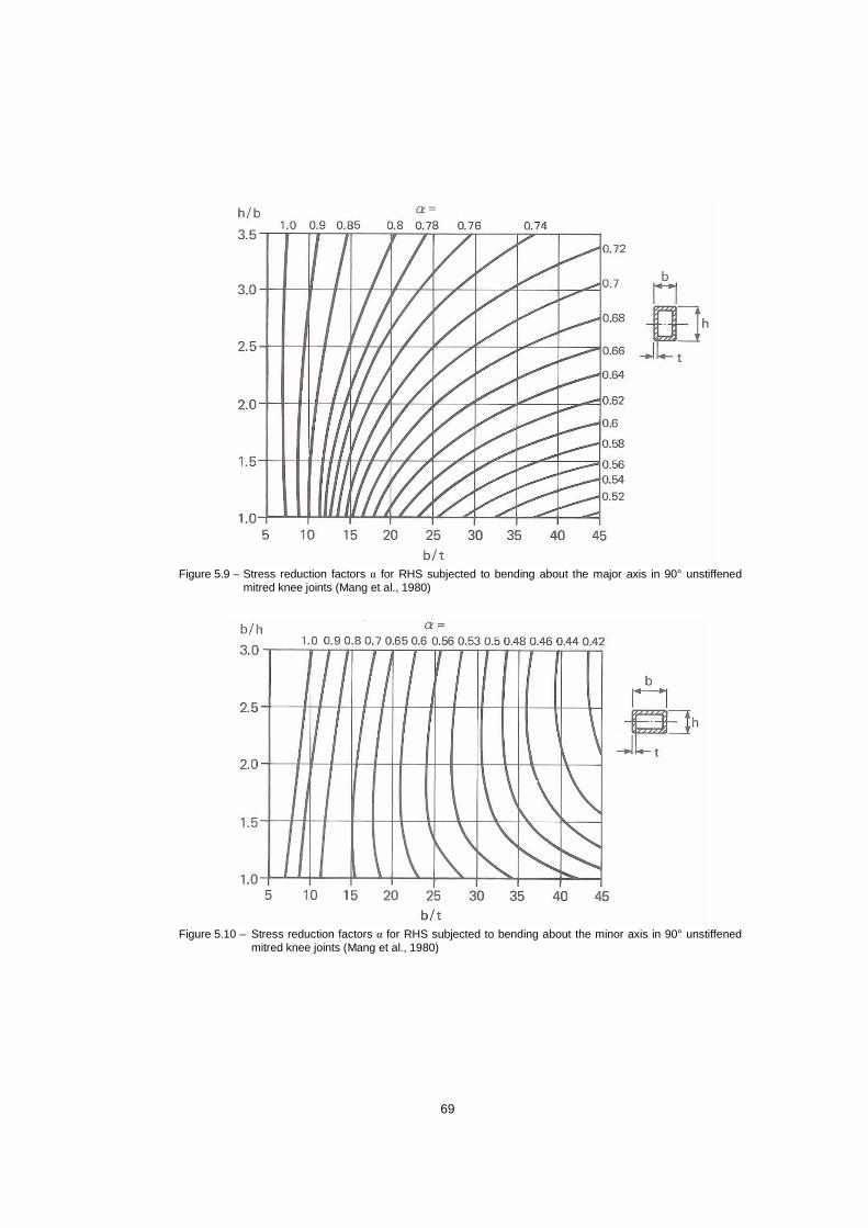
69

Figure 5.9 – Stress reduction factors α for RHS subjected to bending about the major axis in 90° unstiffened

mitred knee joints (Mang et al., 1980)

Figure 5.10 – Stress reduction factors α for RHS subjected to bending about the minor axis in 90° unstiffened

mitred knee joints (Mang et al., 1980)

70

6 Multiplanar welded joints Multiplanar joints are frequently used in tubular structures such as towers, space frames, offshore structures, triangular trusses (Delta trusses), quadrangular trusses and many other applications. Triangular trusses, as illustrated in figure 6.1, have several advantages over single plane trusses, such as the increased lateral stability offered by the twin, separated, but connected compression chords. They are frequently used as exposed structures and considered equivalent in appearance, but less expensive than space frames. Furthermore, in general, purlins are not necessary with triangular trusses, as the usual practice is to space the top chords of the trusses at a distance suitable for the roof deck, and then fasten the roof deck directly to the flat surfaces of the RHS top chords.

Figure 6.1 – RHS triangular truss with double compression chords 6.1 KK joints Initial tests by Coutie et al. (1983) on RHS multiplanar KK joints found a small decrease compared to the strength of the in-plane K joint due to out-of-plane loaded brace members. Bauer and Redwood (1988) deduced that for KK joints to the single RHS chord of a triangular truss, as shown in figure 6.1, there was little interactive effect produced by identical loading (same sense) on an adjacent wall of the chord.

2N1

φ

N1 N1

Figure 6.2 – Elevation view of a KK joint to triangular truss tension chord As further failure modes may exist over a wider range of joint parameters than those studied by Coutie et al. (1983) and Bauer and Redwood (1988), in the 1st edition of this Design Guide (Packer et al., 1992) it was suggested to use a reduction factor of 0.9 in conjunction with the uniplanar K joint design formulae (see table A7 of Appendix A). This applied to cases where the angle between brace member planes φ was equal to or less than 90° and with the brace members attached to the chord face with no eccentricity, as illustrated in figure 6.2. This was the same reduction factor as given for CHS KK joints in the 1st edition of CIDECT Design Guide No. 1 (Wardenier et al., 1991).

71

The recommendation for RHS KK joints in the 1st edition of this Design Guide (Packer et al., 1992) was made for 60° ≤ φ ≤ 90°. In addition, it was advised always to perform a chord shear check for gap KK joints, as shown in table A7 of Appendix A. Since then, extensive analytical and numerical research has been carried out by Liu and Wardenier (2001a, 2001b, 2002, 2003). It was concluded that the differences in capacity between uniplanar K gap and multiplanar KK gap joints are caused by the different chord force. Based on this work, the following recommendations can be made, summarized in table 6.1: Multiplanar KK gap joints: - For chord face plastification (small or medium β), the strength of the joint can be based on the

joint resistance formulae for uniplanar joints given in tables 4.1 and 4.2, and no further multiplanar correction is necessary, provided that the actual total chord force is used for the chord stress function Qf.

- For large β ratios or rectangular chord sections, the strength of a KK gap joint is governed by

chord shear and chord axial force interaction, presented in table 6.1. The K gap joint (with φ = 90°)

is subjected to a shear force of gap,0 V20.5 in each plane, where Vgap,0 is the total “vertical”

shear force. The shear force in each plane is resisted by the two walls of the RHS chord. The horizontal components from the two planes equilibrate.

Multiplanar overlap KK joints: - For multiplanar overlap KK joints, the strength of the joint is similar to the current

recommendations for uniplanar overlap joints in table 4.3. Thus, compared to the previous recommendations in the 1st edition of this Design Guide (Packer et al., 1992), a brace shear criterion and a local chord yielding criterion have been added.

Multiplanar RHS KK gap joint

72

6.2 TT and XX joints Initial, theoretical research by Davies and Morita (1991) on TT and XX joints showed that little difference exists between the design strengths of planar and multiplanar 90° TT and XX joints. Because of a lack in experimental evidence, the 1st edition of this Design Guide recommended to apply a correction factor of 0.9 to the uniplanar T and X joint resistances to account for out-of-plane loaded braces (see table A7 of Appendix A). Extensive research by Yu (1997) on XX and TT joints revealed that the multiplanar effect is caused by geometric and loading effects. The geometric effect is a function of the width ratio β and the chord width-to-thickness ratio 2γ, with β as the most important influence. Based on Yu’s work, table 6.1 gives simplified recommendations for multiplanar TT and XX joints.

Erection of an RHS pipeline bridge

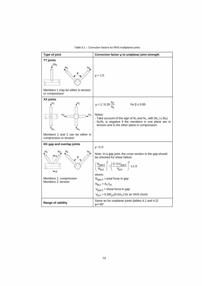
73

Table 6.1 – Correction factors for RHS multiplanar joints

Type of joint Correction factor µ to uniplanar joint strength

TT joints 2N1

φ

N1 N1

Members 1 may be either in tension or compression

µ = 1.0

XX joints N1

N2

N1

N1 N1

N2

Members 1 and 2 can be either in compression or tension

1

2

NN

35.01+=µ for β ≤ 0.85

Notes: - Take account of the sign of N2 and N1, with |N1 | ≥ |N2| - N2/N1 is negative if the members in one plane are in

tension and in the other plane in compression.

KK gap and overlap joints

A

A

φ

N1 N1N1 N2

Members 1: compression Members 2: tension

µ =1.0 Note: In a gap joint, the cross section in the gap should be checked for shear failure:

0.1V

V71.0

N

N2

0,pl

0,gap 2

0,pl

0,gap ≤

+

where: e in gapaxial forcNgap,0 =

y0 0pl,0 fAN =

in gapforceshear Vgap,0 =

)A5.0(f58.0V 00y0,pl = for an SHS chord

Range of validity Same as for uniplanar joints (tables 4.1 and 4.2) φ ≈ 90°

74

7 Welded plate-to-RHS joints Branch plate joints are one of the most popular joint types due to their ease of fabrication and handling. Originally, longitudinal branch plate joints were used with I section beams or columns with the branch plate welded along the centre of the flange, so that the force introduced by the branch plate was directly transmitted to the web of the I section. This practice was carried over to hollow section construction, but then the branch plate was attached in a similar manner to the middle of the hollow section face which is very flexible and often deforms excessively, frequently exceeding the deformation limit at relatively low loads. For welded RHS joints, a serviceability deformation limit of 1% and an ultimate deformation limit of 3% of the width of the connecting chord face (0.03b0) have been employed, as it has been shown that this ultimate deformation limit reasonably corresponds to the yield load of these joints (Lu et al., 1994). Besides the yield strength or deformation criteria, punching shear of the hollow section connecting face is a further critical limit state which has to be checked, among others. All pertinent limit state checks are summarized in table 7.1 and are further explained below. Generally, the presented formulae have been simplified by considering only loads perpendicular to the hollow section member and disregarding the (generally positive) effect of fillet welds. The orientation (longitudinal or transverse) and width of the branch plate has a major effect on the strength and failure mode of branch plate joints. Hence, the following discussion distinguishes between the longitudinal and transverse plate joints. 7.1 Longitudinal plate joints under axial loading Due to their very low β ratios, longitudinal plate-to-RHS joints tend to have excessive distortion or plastification of the RHS connecting face. An analytical approach is used to predict the limit state of chord face plastification and is based on a flexural model using yield line analysis (Cao et al., 1998a, 1998b). The influence of compressive stress in the RHS chord member, either due to axial load or bending moment, has been taken into account by the term Qf. In table 7.1 this term is the result of recent research to harmonize the chord stress effects on RHS and CHS welded joints (Wardenier et al., 2007a, 2007b). If the longitudinal plate is loaded by an axial force that is not at 90° to the RHS member axis, the joint resistance can be evaluated using the normal component (N1 sin θ1). The foregoing design recommendation has been validated by research in which the longitudinal branch plate was located along the RHS member axis. A slight variant is sometimes produced when the longitudinal branch plate is offset from the RHS centreline so that the centreline of the connected member can coincide with that of the RHS. This should cause minimal difference in behaviour of the RHS face and this detailing arrangement is also acceptable. However, as noted in the last paragraph of section 7.6, for eccentrically-connected lap splice plates under compression loading, the effect of the eccentricity must be taken into account in the design of both connected plates. 7.2 Stiffened longitudinal plate joints under axial loading Longitudinal plate-to-RHS joints in particular are only suitable for lightly loaded branch plates, so methods of strengthening this joint type have been examined. Research on longitudinal through-plate joints (Kosteski, 2001; Kosteski and Packer, 2003b) verified the assumption that a through-plate joint has approximately double the resistance of a simple longitudinal branch plate joint, which is reflected in the design equation for this joint type in table 7.1. This is because of the plastification of two RHS walls rather than one. While the single plate joint is one of the least expensive plate-to-RHS joints, the through-plate joint is deemed to be the most expensive because of the slotting procedure (Sherman, 1996). Designers should also bear in mind that a part of the through-plate protrudes beyond the far side of the RHS (see table 7.1) and this may affect joints to that face of the RHS.

75

Another means of strengthening a longitudinal plate joint is to use a stiffened longitudinal plate (T stub) to RHS joint. By adding the stiffening plate at the end of the branch plate, the “footprint” of the branch becomes much enlarged (an increased β ratio). Provided that the stiffening plate is rigid enough, the stiffened longitudinal plate-to-RHS joint can then be regarded as a RHS-to-RHS T joint, whereby the width of the stiffening plate becomes the new width of the “branch/brace member”. Based on work by Kosteski (2001) and Kosteski and Packer (2003a) a minimum thickness was derived for the stiffening plate to ensure the required rigidity (see table 7.1). 7.3 Longitudinal plate joints under shear loading This type of joint is primarily found in “simple” shear joints to hollow section columns, where the plate is typically referred to as a “shear tab” or “fin plate”. Over a wide range of joints tested by Sherman (1995, 1996) only one limit state was identified for the RHS member. This was a punching shear failure related to end rotation of the beam when a thick shear tab was connected to a relatively thin-walled RHS. A simple criterion to avoid this failure mode is to ensure that the tension resistance of the tab under axial load (per unit plate length) is less than the shear resistance of the RHS wall along two planes (per unit plate length). This is achieved if (Sherman, 1995):

0yp

0yp t

f

f16.1t < 7.1

This design check is valid for RHS members that do not have slender cross sections (i.e. which are not thin-walled; i.e. are not class 4 according to Eurocode 3 (CEN 2005a)). Further details regarding this design criterion, along with a design example, are provided in CIDECT Design Guide No. 9 (Kurobane et al., 2004), where a variant of the above equation is used, basing the shear resistance instead on shear ultimate stress of the RHS wall rather than shear yielding. 7.4 Transverse plate joints under axial loading 7.4.1 Failure mechanisms Joints with transverse plates typically have higher β values than comparable joints with a longitudinal branch plate. Thus, they are less flexible and can have different failure mechanisms than joints with a longitudinal plate. For branch plate-to-RHS joints with transverse plates, four basic failure mechanisms have now been identified, with each limit state having the potential to govern in the plate-to-RHS width ratio (β) ranges stipulated below (see table 7.1):

- Chord face plastification (for 0.4 ≤ β ≤ 0.85) - Chord punching shear (for 0.85 ≤ β ≤ 1-1/γ) - Chord side wall failure (for β ≈ 1.0) - Local yielding of the plate (for all β) Initial research on transverse branch plate joints to RHS was carried out by Wardenier et al. (1981) and Davies and Packer (1982). Davies and Packer observed a combination of flexural failure and punching shear for joints with high β values (but slightly less than 1-1/γ). Based on the work of Wardenier et al. (1981), an effective punching shear width of the branch member was introduced, which was incorporated into a standard punching shear model. A similar effective branch width was further used to calculate the local yielding strength of the branch. Chord face plastification was initially deemed a non-critical failure mode, for all transverse plate joints, and was hence omitted as a design check in the 1st edition of CIDECT Design Guide No. 3 (Packer et al., 1992). Plastification of the connecting chord face is well represented by the formation of a yield line mechanism. Lu (1997), however, subsequently found that the yield capacity of the connecting RHS face could be severely lowered in the presence of high normal compressive stresses in the connecting chord face. Lu hence determined an appropriate reduction factor, Qf, and the application of this – for high RHS compression stresses – may make the chord face

76

plastification failure mode critical. Hence, this failure mode was introduced into CIDECT Design Guide No. 9 (Kurobane et al., 2004). The limit state expression used herein for this failure mode is a result of recent reanalyses by Wardenier et al. (2007a, 2007b). For transverse plates in which the width of the plate is about the width of the chord or hollow section (β ≈ 1.0), the plate will bear directly on the RHS side walls. In this case, chord side wall failure is the pertinent failure mode for which the joint must be designed. The chord side wall failure stress is taken as the yield stress because the plate applies the compression load in a very localised manner. However, Lu (1997) has also noted that the chord side wall failure resistance can also be decreased by compressive normal stresses in the RHS if the hollow section has a high h0/t0 value. Hence, a Qf chord stress term has been included with this limit state expression. 7.4.2 Design of welds The non-uniformity of load transfer along the line of weld, due to the flexibility of the RHS connecting face in a transverse plate joint, must be taken into account in proportioning such welds. This can be satisfied by limiting the total effective weld length (between the plate and RHS) to 2be, as defined in table 7.1, where the factor 2 accounts for welds on both sides of the transverse plate. An upper limit on weld size will be given by the weld that develops the full yield strength of the connected transverse plate (A1fy1), which then ensures that the weld is non-critical. Even if one uses just a particular length of weld as being effective, for weld design purposes, the actual weld should have the same weld size and extend over the entire plate width (b1).

Complex joint in the Rogers Centre, Toronto, Canada

77

Table 7.1 – Design resistances of uniplanar branch plate-to-RHS joints

Type of joint Design limit state

T and X joints – transverse plate

t1

h0

N1

t0

b1

b0

t1

h0

N1

N1

t0

b1

b0

Chord face plastification (for 0.4 ≤ β ≤ 0.85)

f 2 0 y0

*1 Q

9.01

8.22tfN

β−β+=

Chord punching shear (for 0.85 b0 ≤ b1 ≤ b0 – 2t0)

)2bt2(t0.58fN pe,1 0 y0*1 +=

Chord side wall failure (for β ≈ 1.0) (*)

f 01 0 y0 *1 Q)5tt(tf2N +=

Local yielding of plate (for all β)

e 1 1y*1 btfN =

T and X joints – longitudinal plate

h1

h0

t1

b0

t0

N1

h1

h0

t1

t0

b0

N1

N1

Chord face plastification

f0

12 0 0y *

1 Qbt

12tf2N

−+η=

(*) For 0.85 < β < 1.0, use linear interpolation between the resistance for chord face plastification at β = 0.85 and the resistance for chord side wall failure at β = 1.0.

78

Table 7.1 – Design resistances of uniplanar branch plate-to-RHS joints (continued)

Type of joint Design limit state

T joints - longitudinal through-plate

h1

h0

t1

b0

t0

N1

Chord face plastification

f 0

12 0 0y

*1 Q

bt

12tf 4N

−+η=

T stub joints - stiffened longitudinal plate

h1

h0

t1

t0

N1

b0

bsp

tsp

*3 0sp et5.0t β≥

00

1sp*

tb

tb :with

−−

=β

If tsp fulfils the above requirement, the joint can be regarded as an RHS-to-RHS T joint. In the design equations for RHS-to-RHS T joints, the stiffening plate width bsp is then used for the branch width b1.

Function Q f

1Cf )n(1Q −= with

0,pl

0

0,pl

0

MM

NN

n += in connecting face

Chord compression stress (n < 0)

Chord tension stress (n ≥≥≥≥ 0)

Transverse plate C1 = 0.03γ but ≥ 0.10 C1 = 0.10

Longitudinal plate C1 = 0.20

Factors

be and b e,p 111 y1

0 y0

00e bbut b

tf

tf

/tb10

b ≤

= 11

00p,e b but b

/tb10

b ≤

=

Range of validity

RHS chord

Compression class 1 or 2 40/th and 40 /tb and 0000 ≤≤

Tension 40/th and 40/tb 0000 ≤≤

Aspect ratio 0.2/bh5.0 00 ≤≤

Transverse plate 4.0/bb 01 ≥=β

Longitudinal plate 4/bh1 01 ≤=η≤

Plate angle o901 ≈θ

Yield stress y0y1 ff ≤ uy f8.0f ≤ fy ≤ 460 N/mm2 (**)

(**) For fy0 > 355 N/mm2, see section 1.2.1

79

7.5 Gusset plate-to-slotted RHS joints Single gusset plates, slotted into the ends of hollow section members and concentrically aligned with the axis of the member, as shown in figures 7.1 to 7.3, are commonly found in diagonal brace members of steel framed buildings (see figure 7.4) and also in roof brace-to-chord member joints. Slotted RHS joints are noted by the presence (or lack) of an open slot at the end of the slotted RHS. An open slot allows for liberal construction and fabrication tolerances, if the longitudinal welds are performed on site. If the gusset plate bears against the end of the slot (common for shop fabrication) the ends of the gusset plate are typically welded with “end return welds”. As a consequence of only part of the RHS cross section being connected, an uneven stress distribution around the RHS perimeter always occurs during load transfer at the connection. This phenomenon, known as shear lag, is illustrated in figure 7.1. Figure 7.1 – Shear lag in gusset plate-to-slotted RHS joints Two possible failure modes have been identified for gusset plate-to-slotted RHS joints loaded in tension: circumferential failure (CF) of the RHS (see figure 7.2) and tear out (TO) – or “block shear” – failure of the RHS (see figure 7.3). Shear lag is principally influenced by the weld length, Lw, or the “stick-in length”. For long weld lengths, shear lag effects become negligible, while for short weld lengths (Lw/w < 0.7), tear out governs over circumferential fracture of the RHS, where the dimension w is the distance between the welds measured from plate face-to-plate face, around the perimeter of the RHS. For both cases shown in figure 7.2, Martinez-Saucedo and Packer (2006) have shown that the RHS circumferential failure limit state design resistance in tension can be determined by:

+

−=7.5 4.2

w

ui n*i

wL

1

11fA9.0N for Lw / w ≥ 0.7 7.2

For the RHS tear out limit state (see figure 7.3), the design resistance in tension can be determined by summing the fracture resistance of the net area in tension and the resistance of the gross area in shear (Martinez-Saucedo and Packer, 2006):

Stress trajectory

An < Ag

TOP

SIDE

80

++=

2

ffA58.0fA 9.0N uiyi

gvuint*i for Lw / w < 0.7 7.3

Note that for the gusset plate-to-slotted RHS with longitudinal welds only, as shown in figure 7.3(a), Ant is 0 mm2. Depending on the weld length, Lw , only one of these two limit states (failure modes) needs to be checked (unlike in many contemporary steel specifications). The 0.9 factor in these equations represents a 1/ γM = φ term, determined by a reliability analysis. As indicated in figure 7.2(a) and figure 7.3(a), when there is an opening at the end of the slot, cracking starts at the end of the weld. Thus, under static loading, the cutting of the slot end does not need to be smooth, drilled or machined, and some roughness is tolerable. (Under dynamic loading conditions the slot end should be very smooth). For these joints in compression, the member axial load is limited by overall buckling of the brace and hence, the member compression load is typically well below the capacity of the joint in compression.

An

Lw

An=Ag

a)

crack

slot

GussetPlate b)

RHS

crack

RHSLw

Figure 7.2 – Gusset plate-to-slotted RHS joints: Circumferential failure (CF) with: (a) longitudinal welds only and

(b) longitudinal welds plus a weld return

Ant

a)

crack

GussetPlate b)

RHS

RHS

crack

AgvAnt

Ant

Agv

Figure 7.3 – Gusset plate-to-slotted RHS joints: Tear out (TO) failure with: (a) longitudinal welds only (Ant = 0)

and (b) longitudinal welds plus a weld return

81

Figure 7.4 – Gusset plates slotted into a diagonal RHS bracing member, in a braced steel frame 7.6 Tee joints to the ends of RHS members When an axial force is applied to the end of an RHS member, via a welded Tee joint as shown in figure 7.5, the possible limit state for the RHS is yielding of the walls (due to applied tension or compression loads). Also, the resistance of the RHS needs to be computed with consideration for shear lag. In general, the RHS could have dimensions of b1 x h1, but figure 7.5 shows the bearing width, tw, oriented for lateral load dispersion into the RHS wall with dimension b1. A conservative assumption for the distribution slope is 2.5:1 from each face of the Tee web (stem) (Kitipornchai and Traves, 1989), which produces a dispersed load width of (5tp + tw). It is proposed to use this effective width around the perimeter of the RHS member. This is also adopted for CHS members in CIDECT Design Guide No. 1 (Wardenier et al., 2008). Thus the resistance of the RHS can be computed by summing the contributions of the parts of the RHS cross sectional area into which the load is distributed:

1y 1pw 1 y1 *1 fA)5t(ttf2N ≤+= 7.4

A similar load dispersion can be assumed for the capacity of the Tee web. If the web has the same width as the width of the cap plate, i.e. (h1 + 2s), the capacity of the Tee web is:

)s5t.2(ttf2N p1w yw *1 ++= 7.5a

)5t(ttf2 p1w yw +≤ 7.5b

In equations 7.4 and 7.5, the size of any weld legs to the Tee web (stem) has been conservatively ignored. If the weld leg size is known, it is acceptable to assume load dispersion from the toes of the welds. If the applied load N1 (figure 7.5) is compressive, it is assumed that the RHS does not have a slender cross section (i.e. is not class 4).

82

N1 N1

tp tw

t1

b1 s h1 s

5tp+tw

2.5 1

Figure 7.5 – Load dispersion for a Tee joint on the end of an RHS member Tee joints to the ends of RHS members usually have the web (stem) centred on the RHS member axis, but connection is then frequently made to a single gusset plate, usually by bolting. In such situations a bending moment is induced in the joint by the eccentricity between the plates which must be considered. Under compression loads, the gusset plate and the Tee web (stem) should be proportioned for axial load and bending moment, assuming that both ends of the connection can sway laterally relative to each other. These comments also apply to the proportioning of other plates covered in chapter 7, when the plate is loaded in compression but connected by a lap splice eccentrically to another single gusset plate.

83

8 Bolted joints Bolting directly to RHS members is a concern, due to lack of access to the interior of the member (other than near the ends). Welding attachments to the RHS and then bolting remote to the section is a popular option, and normal joint design principles – given in all national and international steel structures codes/specifications – are applicable. Examples of this technique, using angle, fork, channel, tee and plate welded attachments, are given in figure 8.1. Bolted joints are particularly useful for connecting prefabricated sub-assemblies on site and for truss-to-column joints (see figure 8.2).

(a) (d)

(b) (e)

(c) (f)

Figure 8.1 – Examples of bolted joints to RHS ends, using welded attachments

(a) (b)

(c)

Figure 8.2 – Examples of bolted joints at the ends of RHS trusses If fastening directly to the RHS wall, several types of mechanical fasteners that can be used are: through-bolts, blind bolts, flow-drilling, welded-on threaded studs and screws. Fasteners can generally be categorized as either loaded in shear or loaded in tension (although a combination of both sometimes occurs); examples of each are shown in figure 8.3 for direct fastening to RHS. Many more details about direct fastening methods to hollow sections are given in CIDECT Design Guide No. 7 (Dutta et al., 1998).

I section (RHS-stub also possible)

RHS-stub (I section also possible)

plate

84

(a) A splice joint in a double chord truss where the bolts (loaded in shear) have been tightened with the aid of access holes

(b) A beam-to-column end-plate joint under moment loading, where the bolts (loaded in tension) are blind bolts

Figure 8.3 – Examples of direct fastening to RHS 8.1 Flange-plate joints Flange-plate joints, as shown in figure 8.1(c), are a very popular means of joining the ends of RHS together, whether by bolting on two sides of the RHS or by bolting on all four sides of the RHS. Design procedures for both of these options are given in the following sections, for axial tension loading on the RHS member. In such joints the high-strength bolts should be fully pre-tensioned, particularly if there is any dynamic loading on the joint. Under axial compression loading, the bolts will be non-critical and the flange-plates will be in bearing. A method for handling axial load plus bending moment on the RHS member is given in section 8.1.3. 8.1.1 Bolted on two sides of the RHS – tension load ing Preliminary tests on flange-plate joints bolted along two sides of the RHS were performed by Mang (1980) and Kato and Mukai (1985) followed by a more extensive study by Packer et al. (1989), illustrated in figure 8.4. The latter tests showed that one could, by selecting specific joint parameters, fully develop the tensile resistance of the member by bolting along only two sides of the RHS. This form of joint lends itself to analysis as a two-dimensional prying problem, and a modified T stub design procedure, based on that of Struik and de Back (1969), has been advocated to evaluate the joint limit states (Packer and Henderson, 1997).

Figure 8.4 – Tension test of a flange-plate joint bolted along two RHS sides, showing plate flexure

85

In order for the design criteria to be valid, the centreline of the bolts in the flange-plate joint should not be positioned beyond the corner of the RHS. The limit states for the flange-plate joint, bolted on two sides, are:

- yielding of the end plate - tensile strength of the bolts, including prying action - strength of the weld connecting the flange-plate to the RHS Important geometric parameters are illustrated in figure 8.5. Most codes/specifications stipulate bolts with tensile loads be fully pretensioned. This is an essential requirement for any dynamic loading situation. It has been shown that spacers placed between the flange-plates, in line with the RHS walls and parallel to the bolt lines, can preclude prying action and improve fatigue performance (Bouwman, 1979).

tp

ab

ti

bi

pp p

Boltholediameterd’tp

ab

ti

bi

pp p

Boltholediameterd’tp

ab

ti

bi

pp p

Boltholediameterd’

Figure 8.5 – Rectangular flange-plate joint with bolts along two sides of RHS The modified T stub design procedure (Birkemoe and Packer, 1986) involved a redefinition of some parameters to reflect the observed location of the inner (hogging) plastic hinge line and to also represent the joint behaviour exhibited by more complex analytical models. The distance b (shown on figure 8.5) was adjusted to b’, where:

b’ = b - (d/2) + ti 8.1

The term α has been used in Struik and de Back’s T stub prying model to represent the ratio of the (sagging) bending moment per unit plate width at the bolt line, to the bending moment per unit plate width at the inner (hogging) plastic hinge. Thus, for the limiting case of a rigid plate, α = 0, and for the limiting case of a flexible plate in double curvature with plastic hinges occurring both at the bolt line and the edge of the T stub web, α = 1.0. Hence, the term α in Struik and de Back’s model was restricted to the range 0 ≤ α ≤ 1.0. For bolted RHS flange-plate joints, this range of validity for α was changed to simply α ≥ 0. This implies that the sagging moment per unit width at the bolt line is allowed to exceed the hogging moment per unit width, which was proposed because the RHS member tends to yield adjacent to the hogging plastic hinge and participate in the general failure mechanism. This behaviour is confirmed by the inward movement of the hogging plastic hinge (see figure 8.4). Thus, a suitable design method for this joint type follows below. A design example, that also follows these steps, is given in section 10.5. 1. Estimate the number n, grade and size of bolts required, knowing the applied tensile force Ni

and allowing for some amount of prying. In general, the applied external load per bolt should be only 60% to 80% of the bolt tensile resistance in anticipation of bolt load amplification due to prying. Hence, determine a suitable joint arrangement. The bolt pitch p should generally be about 4 to 5 bolt diameters (although closer pitches are physically possible if required), and the edge distance a about 1.25b, which is the maximum allowed in calculations. Prying decreases

86

as the edge distance a is increased up to 1.25b, beyond which there is no advantage. Then, from the joint layout, determine the ratio of the net plate area at the bolt line to the gross plate area at the hogging hinge line:

pd'

-1=δ 8.2

where: d’ = the bolt hole diameter p = the length of flange-plate tributary to each bolt, or bolt pitch (see figure 8.5). Determine a trial flange-plate thickness tp from:

f pf

KPt 1

KP≤≤

δ+ 8.3

where ==nN

P if the external factored tensile load on one bolt (n is the number of bolts), and

pf10 b' 4

K yp p

3

φ= (fyp in N/mm2 or MPa) 8.4

where φp = flange-plate resistance factor = 0.9 = 1/ γM.

2. With the number, size and grade of bolts preselected, plus a trial flange-plate thickness, calculate the ratio α necessary for equilibrium by:

( ) 0 but tba )d/2(a

1t

TK

i

2p

* ≥

++δ+

−=α 8.5

where T* is the factored tensile resistance of one bolt. Note that the bolt tensile resistance is used in equation 8.5, because the actual total bolt force Tf, is unknown.

3. Calculate the joint factored resistance *iN by using α from equation 8.5:

( )i

2 p*

i N but K

n 1tN ≥

δα+= 8.6

where n is the number of bolts. The actual total bolt tension, including prying, can be calculated by:

* ff T but

1 'a'b

1PT ≤

δα+δα+≈ 8.7

where: Tf = the total bolt tension a’ = aeffective + d/2 8.8 aeffective = a but ≤ 1.25b (see figure 8.5)

The α value for use in equation 8.7 is given by:

δ

−=α 1

1t

PK

2p

f 8.9

This design method was validated experimentally and analytically (Birkemoe and Packer, 1986; Packer et al., 1989) over a flange-plate thickness range from 12 to 26 mm. It should be borne in

87

mind that when a joint with bolts in tension is subject to repeated loads, the flange-plate must be made thick enough and stiff enough so that deformation of the flange is virtually eliminated (α ≈ 0). 8.1.2 Bolted on four sides of the RHS – tension loa ding Research projects on flange-plate joints bolted along all four sides, as in figure 8.6, have been undertaken by Mang (1980) and Kato and Mukai (1985), but a reliable joint design procedure was not generated. Kato and Mukai proposed a complex model based on yield line theory with an estimate of the prying force. Depending on the relative strengths of the flange plate to the bolts, the ultimate strength of the joint was determined by one of six failure modes. Failure modes 1 to 3 involved failure of the flange plates, while modes 4 to 6 involved bolt failure. However, Kato and Mukai’s method for proportioning flange-plate thickness does not consider the plate yield strength; furthermore, later tests showed that this model could even overestimate the strength by 25% (Caravaggio, 1988). A thorough study of this type of bolted joint has recently been undertaken by Willibald et al. (2001, 2002, 2003a). An analysis of three-dimensional prying action and plate curvature is complex (see figure 8.7), but this work revealed that RHS flange-plate joints bolted on all four sides could still be proportioned on the basis of the two-dimensional T stub prying model of Struik and de Back (1969), with some minor modifications. Following the procedure in section 8.1.1, the inner yield lines in the flange-plate can now be expected adjacent to the RHS outer face and hence the term ti should be deleted from equation 8.1. If the RHS is not square, or if the bolting layout is not the same on all four sides, then the bolt pitch (or the length of flange-plate tributary to each bolt) used should be the minimum of the bolt pitch for the long and the short side (assuming equal values of a and b for the long and short sides). Thus, the bolt pitch to be used is the minimum of p and p’ in figure 8.6. This “minimum p” value is then used in equations 8.2 and 8.4 and the joint analysis then proceeds on the basis of a two-dimensional prying model. In order for this design model to be valid, the centres of the bolt holes should not be positioned beyond the corners of the RHS (as illustrated in figure 8.6). Hence, the bolts should be positioned near the RHS walls, where the tension load acts, not at the plate corners. Also, the range of experimental verification covered joints with up to 10 bolts, RHS up to 254 mm in size, and RHS aspect ratios up to 1.7.

tp

pp

ab

Bolt hole diameter d’

p'

p'

tp

pp

ab

Bolt hole diameter d’

p'

p'

tp

pp

ab

Bolt hole diameter d’

p'

p'

Figure 8.6 – Rectangular flange-plate joint with bolts along four sides of RHS

88

Figure 8.7 – Tension test of a flange-plate joint bolted along four RHS sides (four bolts; thin plates) When two or more bolts are used along one side of an RHS, the distance between adjacent bolts, c, should be as low as possible. (The dimension c is also illustrated in section 10.5). Figure 8.8 illustrates that as the ratio c/hi decreases (where hi is the depth of the RHS wall adjacent to the bolts), the magnitude of the bolt prying force decreases. This figure further shows the trade-off between thick flange-plates (with low bolt prying) and thin flange-plates (with high bolt prying).

Figure 8.8 – Effect of distance between bolts, c, on one side of an RHS, on the magnitude of prying 8.1.3 Flange-plate joints under axial load and mome nt loading Design methods for bolted flange-plate joints to date have generally been developed for axial tension loading on the RHS member. Frequently, however, hollow sections are subjected to both axial tension load (Ni) and bending moment (Mi). In such cases, a hypothetical “effective” axial load can be computed (Kurobane et al., 2004) for use with the flange-plate joint design procedures given in sections 8.1.1 and 8.1.2:

ii

i

i

i A WM

AN

axial Effective

±= 8.10

0

5

10

15

20

25

0 5 10 15 20 25Flange-plate thickness (mm)

Pry

ing

ratio

(%

)

c/h = 0.46

c/h = 0.92

i

i

89

where: Ai = cross sectional area of the RHS Wi = RHS elastic (or plastic) section modulus This procedure will be conservative as it computes the maximum tensile normal stress in the RHS and then applies this to the whole member cross section. 8.2 Gusset plate-to-RHS joints 8.2.1 Design considerations RHS brace members can be field bolted to gusset plates which have been shop welded to RHS chord members, thus producing bolted shear joints as shown in figure 8.9. Such configurations are an option when transportation constraints compel field joints, and bolting has been selected over site welding. If dynamic loading is a design consideration, this type of joint has an advantage over bolted flange-plate joints in that flange plates must be proportioned to eliminate all prying when fatigue loads are present. In general static load applications, however, the gusset-plate joint is Iess aesthetically pleasing and often more expensive than its flange-plate counterpart. An important limitation to the use of RHS gusset-plate joints is the need to have closely matching member widths. Equal width members may be connected directly as in figure 8.9(a), but the gussets often need to be spread slightly by jacking after welding is complete in order to allow field assembly (since welding contraction tends to pull the gussets inwards). Small width differences can be adjusted by the use of filler plates welded on the sides of the brace member. Larger differences allow the further option of extra shim plates, figure 8.9(b), which can be more convenient in the field.

Figure 8.9 – Bolted RHS gusset-plate joints 8.2.2 Net area and effective net area The concept of gross area, net area and effective net area can be used to describe various failure modes for a tension member with holes or openings and these concepts will be utilized herein. Most codes/specifications have very similar checks, with the resistance or safety factors that are applied sometimes varying. The three basic checks are exemplified by (CSA, 2009):

(1) T* = φ Ag fy (yielding of gross area) 8.11 (2) T* = φu (An fu + 0.58Agv (fy + fu)/2 ) (rupture of areas in tension and shear) 8.12 (3) T* = φu Ane fu (rupture of effective net area, with shear lag) 8.13

90

where φ (= 1/γM in Eurocode 3 (CEN, 2005a, 2005b)) is a resistance factor for ductile yielding which can be taken as 0.9 (CSA, 2009; AISC, 2005) or 1.0 (Eurocode 3). The φu resistance factor for brittle rupture is taken as 0.75 by CSA (2009) and AISC (2005), and 1/γM = 0.80 in Eurocode 3 (CEN, 2005a, 2005b). The net area, An, is the total net area in tension along a potential failure path through the member. The gross area in shear, Agv, represents the total area failing in shear, for the same failure path through the member. Equation 8.12 recognizes that the failure path can incorporate segments loaded in tension, in shear, or even combinations of the two, and thus includes the “block shear” failure mode where a chunk of material tears out of the member. For the segment loaded in shear in equation 8.12, the gross area (ignoring bolt holes) is taken as the critical area and at a failure stress that is an average of 0.58fy and 0.58fu (Driver et al., 2006). An illustrative example of the application of equation 8.12, which includes area segments loaded in tension, shear and a combination thereof, is the gusset plate Y joint in figure 8.10, where the “block shear” area of the gusset plate is calculated from the proposed failure line A-B-C-D-E-F-G-H-J-K-L-M.

- The tension segment, normal to the load (AB) has: An = (g1 - d’/2) t - Shear segments parallel to the load (G to M) have, in total: Agv = Lt - Each inclined segment (CD or EF), subject to both tension and shear, can be treated as quasi-

tension segments with an adjusted net area such that, for each segment: An = (g2 - d’) t + (s2/4g2) t For bolted joints, the effective net area reduced for shear lag, Ane, is the net tensile area An multiplied by a shear lag reduction factor (≤ 1.0). Shear lag applies when a member is connected by some – but not all – of its cross sectional area and the critical failure path includes parts of the unconnected cross section. Thus, equation 8.13 may not always be applicable. It is not applicable, for example, in considering any failure path of the gusset plate in figure 8.10, because the whole “tension member” (the gusset plate) is loaded.

Figure 8.10 – Calculation of net area An (in tension) and gross area Agv (in shear) for a gusset plate The shear lag factor to be applied to An (Ane = shear lag factor x An), is given in most codes/specifications for bolted joints; for example, for CSA (2009) this shear lag factor is:

- 0.90 when shapes like I sections (or tees cut from them) are connected only by their flanges with at least three transverse rows of fasteners (flange width ≥ 2/3 the depth),

- 0.85 for structural shapes such as RHS connected with three or more transverse rows of fasteners,

- 0.75 for structural shapes such as RHS connected with two transverse rows of fasteners.

91

For example, if the brace member in figure 8.10 was an RHS and it was bolted to gusset plates on two sides, as suggested in the figure, with each side having eight bolts in three rows (as shown), then the reduced effective net area, Ane, to be applied to the RHS tension member in equation 8.13 would be 0.85An. In this instance, the net area An would be the gross RHS cross sectional area minus the 2 x 3 bolt holes in the first bolt row. An example of the failure mode of an RHS tension member, bolted to gusset plates along just two RHS sides, is given in figure 8.11.

Figure 8.11 – Tear out failure mode for a bolted RHS (with a hand access hole cut-out) in tension The effective net area reduced for shear lag, Ane, also applies to welded joints when a member is not welded all around its cross section, for example when an element (i.e. a part of the cross section) is connected along its edge(s) by welds parallel to the direction of load. Such a case is illustrated in figure 8.9(b) where bolting plates are welded to the sides of the RHS brace member. For welds parallel to the direction of load (as the four flare groove welds would be in figure 8.9(b), along the four corners of the RHS), the shear lag factor is a function of the weld lengths and the distance between them. The distance between these welds would be bi or hi, for orthogonal sides of the RHS brace. Also, the RHS brace can be reduced to four area elements, with the approximate gross area of the brace being equal to 2t(bi - ti) + 2t(hi - ti). Thus, shear lag reduction factors can be applied to each of the four element areas (two of width w = bi - ti, and two of width w = hi - ti), to produce a total effective net area of the RHS reduced by shear lag, Ane, for use in equation 8.13. Suggested shear lag reduction factors for these four element areas, in terms of the weld length Lw, are (CSA, 2009): - 1.00 when the weld Iengths (Lw) along the RHS corners are ≥ 2bi (or 2hi as applicable) - (0.5 + 0.25Lw/bi ) when the weld lengths along the RHS corners are bi ≤ Lw < 2bi, or - (0.5 + 0.25Lw/hi ) when the weld lengths along the RHS corners are hi ≤ Lw < 2hi - 0.75Lw/bi when the weld lengths along the RHS corners are Lw < bi (or hi as applicable) Section 7.5 of this Design Guide discusses another application of shear lag to welded plate-to-RHS joints, where again the shear lag effect is a function of the weld length divided by the distance between the welds. Another failure that must be checked, in gusset-plate joints such as shown in figures 8.9 and 8.10, is yielding across an effective dispersion width of the plate. This can be calculated using the Whitmore (1952) effective width concept, illustrated in figure 8.12. For this failure mode (for two gusset plates):

92

( )p15.1gtf 2N p yp*i ∑+φ= 8.14

where φ = 0.9 (= 1/γM) is conservative. The term Σp represents the sum of the bolt pitches in a bolted joint or the length of the weld in a welded joint.

Figure 8.12 – Whitmore criterion for gusset-plate yielding or buckling

The use of *iN indicates that this check applies to both tension and compression load cases. If the

member is in compression, buckling of the gusset plate must also be prevented. A suitable method for checking the buckling resistance is given by Thornton (1984). The gusset plate compressive resistance is the column resistance given by an applicable code/specification for a column having a width of (g + 1.15Σp), a depth equal to the gusset-plate thickness, a length equal to the minimum of L1, L2 and L3 and an effective length factor K of 0.65. L1, L2 and L3 (see figure 8.12) are determined by points on the connected edges of the gusset plate, depending on the shape of the gusset plate. 8.3 Hidden bolted joints In some projects, such as where Architecturally Exposed Structural Steel (AESS) has been specified for aesthetic purposes, it may not be possible to have bolts exposed to view, yet the alternative of full site welding may be extremely costly. In such situations, RHS members may be site-bolted together using the technique shown in figure 8.13. Initially, single splice plates are shop-welded into adjoining RHS ends, these are then site-bolted together (preferably keeping the shear plane of the connection coaxial with the two members), and then the joint is finished by adding non-structural cover plates – in the shape of the RHS. Small gaps can be filled with epoxy before painting, thus giving the appearance of a welded joint. Experimental and numerical research on this RHS joint type, under tension loading, has been undertaken by Willibald et al. (2003b). This has confirmed that existing design methods can be used to analyze the pertinent limit states of the RHS, which are:

(1) yielding of the gross area of the cross section (equation 8.11) (2) block shear tear-out of two opposite RHS walls (equation 8.12) (3) fracture of the gross area of the RHS, induced by shear lag (equation 8.13).

93

Access inside the RHS to make adequate welds can be a problem, hence short weld lengths will be typical and welding of the plate to the longer RHS wall will be beneficial. With short weld lengths, block shear tear-out can be expected to become the governing limit state.

(a) Insertion of plate and welding to the RHS (b) Completion with a non-structural cover, after bolting Figure 8.13 – Construction of a hidden bolted joint

94

9 Other uniplanar welded joints 9.1 Reinforced joints Instances may occur when a truss joint has an inadequate resistance, and a designer needs to resort to some form of joint reinforcement. Such a situation might arise if RHS material was ordered on the basis of member selection only, without joint capacity checks being performed. Alternatively, only one or a few joints of a truss may be inadequate due to the selection of a particular chord member, and hence, just these critical joints could be reinforced. The labour costs associated with joint reinforcement are significant, and the resulting structure may lose its aesthetic appeal, but in many cases it may be an acceptable solution. 9.1.1 With stiffening plates The most common method of strengthening RHS joints is to weld a stiffening plate (or plates) to the RHS chord member. It is particularly applicable to gap K joints with rectangular chord members, although an unstiffened overlap joint is generally preferable from the viewpoints of economy and fatigue. However, a gap joint with a stiffening plate eliminates the necessity for double cuts on the brace members, and in certain cases may prove more acceptable to the fabricator. The addition of a flat plate welded to the connecting face of the chord member greatly reduces local deformations of the joint and consequently the overall truss deformations are reduced. It also permits a more uniform stress distribution in the brace members. The type of reinforcement required depends upon the governing failure mode which causes the inadequate joint capacity. Two types of plate reinforcement – in one case to the chord connecting face and in the other to the chord side walls – are shown in figure 9.1. Both of these would be applicable to joints with RHS chord members and either CHS or RHS brace members. An alternative to stiffening a joint with plates is to insert a length of chord material of the required thickness at the connection, the length of which would be the same as Lp given below. This is equivalent to the use of a “joint can” in offshore steel structures, see section 4.6 of CIDECT Design Guide No. 1 (Wardenier et al., 2008).

Figure 9.1 – Pratt truss joint with plate stiffening

(a) Flange plate reinforcement (b) Side plate reinforcement

9.1.1.1 T, Y and X joints Under tension or compression brace loading, the capacity of a T, Y or X joint is typically controlled by either chord face plastification or chord side wall failure, as summarized in table 4.1. When chord face plastification governs, the joint capacity can be increased by using flange plate reinforcement similar to the joint shown in figure 9.1(a). This will usually occur when β ≤ 0.85. When chord side wall failure controls, the joint capacity can be increased by reinforcing with a pair of side plates similar to the joint shown in figure 9.1(b). This failure mode will usually govern when β ≈ 1.0.

95

For T, Y and X joints stiffened with side plate reinforcement, a recommended procedure for calculating the necessary stiffening plate thickness is to use the chord side wall resistance expression in table 4.1, by replacing t0 with (t0 + tp) for the side walls. The stiffening plates should have a length Lp (see figure 9.1(b)), such that for T and Y joints:

1

1p

θsin1.5h

L ≥ 9.1

For T, Y and X joints stiffened with a flange plate, there is a difference in behaviour of the stiffening plate, depending on the sense of the load in the brace member. With a tension load in the brace, the plate tends to lift off the chord member and behaves as a plate clamped (welded) along its four edges. The strength of the joint thereby depends only on the plate geometry and properties, and not on the chord connecting face. Thus, for tension brace loading, if one applies yield line theory to the plate-reinforced T, Y or X joint with rectangular members, the joint factored resistance can be reasonably estimated by the equation for chord face plastification in table 4.1, if

- fy0 is replaced by: fyp - t0 is replaced by: tp - β is replaced by: βp = b1/Bp - η is replaced by: ηp = h1/Bp

where Bp is the plate width. In order to develop the yield line pattern in the stiffening plate, the length of the plate Lp, should be at least:

)bB(B θsin

hL 1p p

1

1p −+≥ 9.2

Also, the plate width Bp should be such that a good transfer of loading to the side walls is achieved; for example Bp ≈ b0 (see figure 9.1(a)). For T, Y and X joints stiffened with a flange plate, and under compression brace loading, the plate and connecting chord face can be expected to act integrally with each other. This type of joint has been studied by Korol et al. (1982), also using yield line theory. Hence for βp ≤ 0.85 (a reasonable upper limit for application of yield line analysis also employed for unreinforced joints), the following plate design recommendations (Korol et al., 1982) are made to obtain a full strength joint:

- Bp ≥ flat width of chord face - Lp ≥ 2b0 - tp ≥ 4t1-t0 The application of the above guidelines, for compression loaded X, T and Y joints, should ensure that the joint capacity exceeds the brace member capacity, provided that chord side wall failure by web crippling is avoided (Korol et al., 1982). 9.1.1.2 K and N joints The capacity of gap K joints is controlled by criteria either related to the chord face or to the chord side wall, as summarized in tables 4.1 and 4.2. When chord face plastification, chord punching shear or local yielding of a brace controls, the joint capacity can be increased by using flange plate reinforcement as shown in figure 9.1(a). This will usually occur when β < 1.0. When chord shear controls, the joint capacity can be increased by reinforcing with a pair of side plates as shown in figure 9.1(b). This failure mode will usually govern when β = 1.0 or h0 < b0. The first design guidance available for K joints stiffened with a flange plate, as shown in figure 9.1(a), was given by Shinouda (1967). However, this method was based on an elastic deformation requirement of the connection plate under specified (service) loads. A more logical limit states approach which is recommended for calculating the necessary stiffening plate thickness for gap K joints is to use the joint resistance expressions in table 4.1 (general), and table 4.2 (for SHS or CHS

96

brace members to SHS chord members) by considering tp as the chord face thickness and neglecting t0. Also, the plate yield stress should be used. It is suggested that proportioning of the stiffening plate be based on the principle of developing the capacity of the brace members (Ai fyi). Dutta and Würker (1988) consider that in most cases this will be achieved providing tp ≥ 2t1 and 2t2. The required thickness can also easily be determined with the design graphs in chapter 4. Careful attention should be paid to the stiffening plate-to-chord welds which should have a weld throat size at least equal to the wall thickness of the adjacent brace member (Dutta and Würker, 1988). The stiffening plate should have a minimum length Lp (see figure 9.1(a)), such that:

++≥

2

2

1

1p

θsinh

gθsin

h 1.5L 9.3

A minimum gap between the brace members, just sufficient to permit welding of the brace members independently to the plate is suggested. All-round welding is generally required to connect the stiffening plate to the chord member, and in order to prevent corrosion on the two inner surfaces. It may also be advisable to drill a small hole in the stiffening plate under a brace to allow entrapped air to escape prior to closing the weld. This will prevent the expanding heated air from causing voids in the closing weld (Stelco, 1981).

Figure 9.2 – Some acceptable and unacceptable, non-standard truss K joints In order to avoid partial overlapping of one brace member onto another in a K joint, fabricators may elect to weld each brace member to a vertical stiffener as shown in figure 9.2(a). Another variation on this concept is to use the reinforcement shown in figure 9.2(b). For both of these joints, tp ≥ 2t1 and 2t2 is recommended (Dutta and Würker, 1988). Designers should note that the K joint shown in figure 9.2(c) is not acceptable, as it does not develop the strength of an overlapped K joint. Also, it is difficult to create and ensure an effective saddle weld between the two brace members. If the capacity of a gap K joint is inadequate and the chord shear criterion is the governing failure mode, then as mentioned before, one should stiffen with side plate reinforcement, as shown in figure 9.1(b). A recommended procedure in this case for calculating the necessary stiffening plate thickness is to use the chord shear resistance expression in table 4.1, by calculating AV as 2h0(t0 + tp). The stiffening plates should again have a minimum length, Lp (see figure 9.1(b)), given by equation 9.3 and have the same depth as the chord member.

97

9.1.2 With concrete filling A less visible alternative to adding stiffening plates to the exterior of an RHS is to fill the hollow section chord with concrete or grout. Filling the chord members of an RHS truss, either along the full length of the chord or just in the vicinity of critical joints, has two main disadvantages: the concrete will increase the dead weight of the structure, and it involves a secondary trade with its associated costs. On the other hand, the strength of certain joints may increase, and if the members are completely filled, there are further benefits of enhanced member capacity (due to composite action), increased truss stiffness and improved fire endurance. Further, as shown in figure 9.3, the joint deformations are considerably reduced.

(a) Unfilled chord (b) Concrete filled chord

Figure 9.3 – K joint with (a) unfilled chord and (b) concrete filled chord Concrete filling of chord members can be done in the fabrication shop by tilting the truss and using a concrete or grout with a high fluidity. The joints which benefit most from concrete filling are X joints with the brace members loaded in compression; i.e. joints at which a compression force is being transferred through the RHS. Examples of such joints are truss reaction points, truss joints at which there is a significant external concentrated load, and beam-to-RHS column moment joints, as illustrated in figure 9.4.

Figure 9.4 – Applications for which concrete filling of RHS may improve the joint resistance Packer (1995) has performed experimental research on a variety of concrete filled RHS joints, resulting in the design recommendations below. The RHS provides confinement for the concrete, which allows it to reach bearing capacities greater than its crushing strength as determined by cylinder compression tests (Packer and Fear, 1991). It has also been shown that a moderate amount of shrinkage of the concrete (or grout) away from the RHS inside walls does not have a negative impact on the strength of a concrete filled joint.

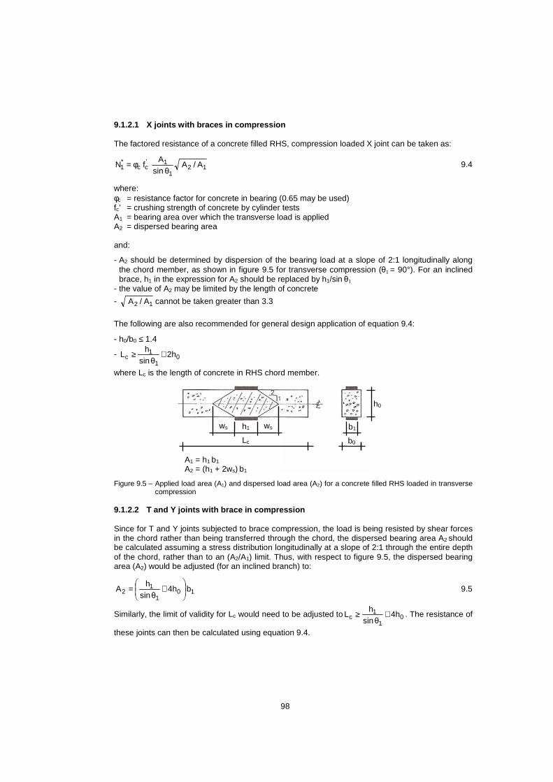
98

9.1.2.1 X joints with braces in compression The factored resistance of a concrete filled RHS, compression loaded X joint can be taken as:

1 2 1

1'c c

*1 A/A

θ sinA

fN φ= 9.4

where: φc = resistance factor for concrete in bearing (0.65 may be used) fc’ = crushing strength of concrete by cylinder tests A1 = bearing area over which the transverse load is applied A2 = dispersed bearing area and:

- A2 should be determined by dispersion of the bearing load at a slope of 2:1 longitudinally along the chord member, as shown in figure 9.5 for transverse compression (θ1 = 90°). For an inclined brace, h1 in the expression for A2 should be replaced by h1/sin θ1

- the value of A2 may be limited by the length of concrete

- 1 2 A/A cannot be taken greater than 3.3

The following are also recommended for general design application of equation 9.4:

- h0/b0 ≤ 1.4

- 01

1c 2h

θsinh

L +≥

where Lc is the length of concrete in RHS chord member. Figure 9.5 – Applied load area (A1) and dispersed load area (A2) for a concrete filled RHS loaded in transverse

compression 9.1.2.2 T and Y joints with brace in compression Since for T and Y joints subjected to brace compression, the load is being resisted by shear forces in the chord rather than being transferred through the chord, the dispersed bearing area A2 should be calculated assuming a stress distribution longitudinally at a slope of 2:1 through the entire depth of the chord, rather than to an (A2/A1) limit. Thus, with respect to figure 9.5, the dispersed bearing area (A2) would be adjusted (for an inclined branch) to:

101

12 b 4h

θsinh

A

+= 9.5

Similarly, the limit of validity for Lc would need to be adjusted to 01

1c 4h

θsinh

L +≥ . The resistance of

these joints can then be calculated using equation 9.4.

ws h1 ws b1

b0

h0

A1 = h1 b1

A2 = (h1 + 2ws) b1

Lc

99

9.1.2.3 T, Y and X joints with brace(s) in tension In tests, none of the concrete filled joints with brace(s) in tension exhibited a decrease in joint yield or ultimate strength, relative to their unfilled counterparts, by more than a few percent. The concrete filled joints still had large joint deformations, so their design should also be based on the joint yield load. Thus, it is recommended that the design capacity of these joints be calculated using existing design rules for unfilled RHS joints (tables 4.1 and 4.2). 9.1.2.4 Gap K joints For the range of joint parameters studied experimentally (Packer, 1995), gap K joints with concrete filled chords were found to have superior joint yield strengths and ultimate strengths relative to their unfilled counterparts. Also, concrete filling of such joints has been found to produce a significant change in joint failure mode, as illustrated in figure 9.3. It is recommended that the joint resistance be calculated separately for the compression brace and the tension brace. For the compression brace, which presses on a relatively rigid foundation of concrete, the joint strength would appear to be limited by bearing failure of the concrete. Hence, calculations should be performed for a Y joint with the brace in compression (see above). For the tension brace, the concrete filling only permits two possible failure modes: (i) premature (local) yielding of the tension brace, and (ii) punching shear of the chord face around the brace. These two failure modes are a subset of the possible limit states experienced with unfilled gap K joints, and resistance formulae are given in table 4.1. 9.2 Cranked-chord joints “Cranked-chord” joints arise in certain Pratt or Warren trusses such as the one shown in figure 9.6 and are characterized by a crank or bend in the chord member at the joint noding point. The crank is achieved by butt (groove) welding two common sections together at the appropriate angle, and the intersection of the three member centre-lines is usually made coincident. The uniqueness of this cranked-chord joint lies both in its lack of a straight chord member and the role of the chord member as an “equal width brace member”.

Figure 9.6 – Cranked-chord joint in a Pratt truss An experimental research programme with SHS and RHS members (Packer, 1991) has revealed that unstiffened, welded, cranked-chord RHS joints behave generally in a manner dissimilar to RHS T or Y joints, despite their similar appearance (they all have a single brace member welded to a uniform-size chord member). Instead, cranked-chord RHS joints have been shown to behave as overlapped K or N joints, and their capacity can be predicted using the criterion for local yielding of the overlapping brace given in table 4.3. Note: the brace shear criterion and the chord yielding criterion based on the interaction of moment and axial load are not applicable here.

100

Thus, cranked-chord joints can be interpreted as overlapped K joints as shown in figure 9.7, wherein one chord member can be given an imaginary extension and the cranked-chord member is considered to be the overlapped brace member. A design example for a cranked-chord joint is given in section 10.4.

Figure 9.7 – Cranked-chord joint represented as an overlapped N joint 9.3 Trusses with RHS brace (web) members framing in to the corners of the RHS chord

(bird-beak joints) With multiplanar or uniplanar RHS trusses, it is also possible to have the truss brace members framing into the corners of an RHS chord member, as shown in figure 9.8. This necessitates very careful profiling of the brace member end, particularly where corner radii are large, into so called “bird-beak”, “bird mouth” or “bill-shaped” joints. Such a member arrangement has been used occasionally in North America, for example in the Minneapolis Convention Center Roof and in the Minneapolis/St. Paul Twin Cities Airport Skyway.

Figure 9.8 – RHS “bird beak” T and K joints It has also been used in Japan, where in this case a robot was developed to profile the ends of the brace members. By framing into the corners of the RHS chord member a high joint strength and stiffness is achieved, regardless of the brace to chord member width ratio. Ono et al. (1991, 1993, 1994) and Ishida et al. (1993) have undertaken experimental studies of such square RHS T and K joints. In their tests, both the chord and braces were rotated through 45° about the member axis, as shown in figure 9.8. All of the 25 T joints tested had the brace loaded in compression, and the 16 K joints had all brace members inclined at θ1 = θ2 = 45° to the chord. It was found that for low to medium β ratios, the “bird beak” joints are much stronger than their conventional RHS counterparts. Ono et al. (1991) and Ishida et al. (1993) concluded that the joint ultimate strengths for axially loaded T joints could be given by:

)f(n' /bb0.9421.794

/tb/bb0.1470.211

1tfN

01

00

01

2 0 y01u

−+

−= 9.6

101

For K joints, however, the equations in their publications differ, whereas no explanation is given. Furthermore, considering the various modes of failure and the many parameters influencing the joint strength, the K joint tests only give an indication for the range investigated. Thus the equations have to be used with care and are only given for indication. As an example, Ono et al. (1991) give for axially loaded K joints:

)f(n'/tb 4 θsin 21

tfN 00

1 2

20 y0

u1 α+

= 9.7

where the effective area coefficient α is given for 45° K joints in figure 9.9. f(n’) is the chord stress function previously used for CHS joints in the 1st edition of CIDECT Design Guide No. 1 (Wardenier et al., 1991) to allow for the influence of normal stresses in compression chords, and is given by:

f(n’) = 1.0 + 0.3n’ - 0.3n’2 for n’ < 0 (chord compression prestress) 9.8a f(n’) = 1.0 for n’ ≥ 0 (chord tension prestress) 9.8b

where n’ = f0p/fy0 9.8c For consistency, it is recommended to use the Qf function of table 4.1 instead of f(n’). As these equations are based on a regression analysis of the test data, one should be careful to ensure that they are only applied within the approximate bounds of parameter ranges examined in the tests, i.e.:

16 ≤ b0/t0 ≤ 42 and 0.3 ≤ b1/b0 ≤ 1.0 for T joints 16 ≤ b0/t0 ≤ 44, 0.2 ≤ b1/b0 ≤ 0.7 and θi ≈ 45° for K joints

Figure 9.9 – Effective area coefficient α, for “bird beak” 45° K joints Further work is reported on T joints loaded by in-plane bending (Ono et al., 1993) and for out-of-plane bending (Ono et al., 1994). These equations also require further investigation and analysis before they can be presented as design recommendations. Davies and Kelly (1995), Davies et al. (1996, 2001) and Owen et al. (1996) investigated several aspects of these bird beak joints numerically, however without proposing design equations.

102

9.4 Trusses with flattened and cropped-end CHS brac e members to RHS chords For statically loaded hollow section trusses of small to moderate span, cropping – a procedure in which a CHS brace member is simultaneously flattened and sheared – can simplify fabrication and reduce cost. The procedure is faster than sawing or profiling, the conventional methods of preparing CHS brace members for welding to RHS and CHS chords, respectively, and it simplifies the welding process. Typical cropped-brace Warren truss joints to an RHS chord member are shown in figure 9.10. Note that the flattened ends of the brace member can be aligned in the direction of the truss or transverse to it. For all trusses with flattened or cropped-brace members, an effective length factor (K) of 1.0 should be used for the design of the brace members.

Figure 9.10 – Cropped-brace joints to an RHS chord Flattening the CHS brace in the plane of the truss (figure 9.10(a)) does not provide as good a structural performance, nor the economies of fabrication, compared to transverse flattening (Grundy and Foo, 1991). Although this has been argued for CHS chord members, the transverse flattening of CHS brace members and welding to RHS chord members is the basis of the “Strarch” roof system (Papanikolas et al., 1990). At this stage, no design guidance is available for such joints to RHS chords. Various types of flattening can be performed on CHS brace members, as illustrated in figure 9.11. In the case of full or partial flattening, the maximum taper from the tube to the flat should remain within 25% (or 1:4). For di/ti ratios exceeding 25, the flattening will reduce the brace member compressive strength (CIDECT, 1984). For welded joints, the length of the flat part should be minimized for compression brace members to avoid local buckling in the flattened region.

Figure 9.11 – Various types of flattening for CHS brace members

103

Considerable research has been performed on in-plane cropped-end CHS braces to RHS trusses by Ghosh and Morris (1981), Morris (1985) and Lau et al. (1985). The latter tests had the geometry shown in figure 9.12, in which the toes of the flattened brace members just met at the chord face, with no overlap or gap between them, and with braces at 45°.

Figure 9.12 – Cropped-brace, zero gap Warren joints For the joint configuration in figure 9.12, with symmetrical brace members, Morris and Packer (1988) showed that the joint resistance is given by:

+

+=

0

1

0

0 y1 *

1 bd

1.711 tb

0.021N0.4N 9.9

where:

- f1' 0

' 1

y0

y1

0'1

'0

'1

'1

1

20 y0

y1 Q tbtanθf

f

t1.32

bb

2hb2θsin

tfN

+

−++π= 9.10

- 00'0 t-bb =

- ='1b width of flattened brace member. (With full cropping and flattening, this can be assumed to

be 2t1. If fillet welding is used, this effective contact width can be increased to include the fillet weld leg dimensions).

- ( )

1

111'1

θsin 2tt-d

h+π=

- =θ'1 slope of brace member face at the cropped end, relative to the chord (see figure 9.12).

Conservatively, a value of 1'1 θ=θ can be used.

Equations 9.9 and 9.10 apply to symmetrical joints where: θ1 = θ2, d1 = d2, t1 = t2, d1/b0 ≥ 0.3 and b0/t0 ≤ 32. 9.5 Double chord trusses Limitations on the largest available RHS member size have restricted the application range of RHS structures. For very long span roof trusses, such as sports centres and auditoria, the use of double RHS chord members will enable longer clear spans than those available from single chord trusses. Immediate advantages of double chord RHS trusses include not only their greater span capacity, but also more efficient and stiffer joints compared to some single chord trusses. Enhanced lateral stiffness can reduce lateral bracing requirements as well as facilitate handling and erection of the structural components.

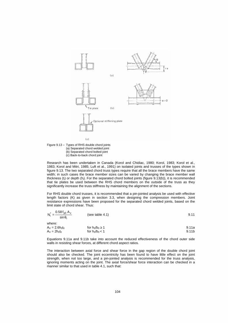
104

Figure 9.13 – Types of RHS double chord joints (a) Separated chord welded joint (b) Separated chord bolted joint (c) Back-to-back chord joint

Research has been undertaken in Canada (Korol and Chidiac, 1980; Korol, 1983; Korol et al., 1983; Korol and Mitri, 1985; Luft et al., 1991) on isolated joints and trusses of the types shown in figure 9.13. The two separated chord truss types require that all the brace members have the same width; in such cases the brace member sizes can be varied by changing the brace member wall thickness (ti) or depth (hi). For the separated chord bolted joints (figure 9.13(b)), it is recommended that tie plates be used between the RHS chord members on the outside of the truss as they significantly increase the truss stiffness by maintaining the alignment of the sections. For RHS double chord trusses, it is recommended that a pin-jointed analysis be used with effective length factors (K) as given in section 3.3, when designing the compression members. Joint resistance expressions have been proposed for the separated chord welded joints, based on the limit state of chord shear. Thus:

i

v y0 *i

θsin

Af0.58N = (see table 4.1) 9.11

where: AV = 2.6h0t0 for h0/b0 ≥ 1 9.11a AV = 2h0t0 for h0/b0 < 1 9.11b Equations 9.11a and 9.11b take into account the reduced effectiveness of the chord outer side walls in resisting shear forces, at different chord aspect ratios. The interaction between axial force and shear force in the gap region of the double chord joint should also be checked. The joint eccentricity has been found to have little effect on the joint strength, when not too large, and a pin-jointed analysis is recommended for the truss analysis, ignoring moments acting on the joint. The axial force/shear force interaction can be checked in a manner similar to that used in table 4.1, such that:

105

2

pl,0

gap,0 y0 vy0 v0

*gap,0gap,0

V

V1fAf)A(2ANN

−+−=≤ 9.12

where: Ngap,0 = axial force in the gap Vgap,0 = shear force in the gap (i.e. Ni sin θi assuming no “purlin load”) A0 = area of one chord member AV is given by equations 9.11a and 9.11b Vpl,0 is given by:

v y0 pl,0 Af0.58V = 9.13

An economic comparison of single chord and double chord RHS trusses (Luft et al., 1991) showed that for short spans, single chord trusses were the lightest and most economical, being around 20% less expensive than back-to-back double chord trusses. (Back-to-back double chord trusses are generally the heaviest and most expensive option for welded trusses.) Thus, for long spans, separated double chord welded joints are preferable and should again prove more economical than back-to-back joints.

Double chord truss

106

10 Design examples 10.1 Uniplanar truss • Truss Iayout and member loads An example has been selected to illustrate the use of the joint design methods given in chapters 4 and 5, as well as the truss design principles described in chapter 3. A Warren truss consisting of SHS members is presented since this configuration is often the preferred solution. A Warren configuration with low brace member angles, such as used here and shown in figure 10.1, keeps the number of joints to a minimum. All members chosen are cold-formed hollow sections with dimensions conforming to EN 10219-2 (CEN, 2006b). The steel grade throughout is S355 with a minimum specified yield strength of 355 N/mm2.

3000 6000 6000 6000 6000 6000 3000

36000

2400

54 kN 108 kN 108 kN

108 kN

108 kN 108 kN 54 kN

38.7° 38.7°

338 878 1148

1080 1215 675

432 432 259 259 86 86

Figure 10.1 – Example Warren truss showing applied loads and resulting member forces (in kN) Figure 10.1 shows the truss and factored loads along with member axial forces, determined by a pin-jointed analysis. The top (compression) chord is considered to be laterally supported at each purlin position. The span-to-depth ratio is 15, which is around the optimal upper limit considering service load deflections and overall costs (section 3.1). • Design of members For member selection, one could use either member resistance tables for the compression members, with the appropriate effective length, or the applicable strut buckling curve or equation. In practice, one would also pay attention to the availability of member sizes selected. For this truss design example, compression member resistance has been determined in accordance with Eurocode 3 (CEN, 2005a) using buckling curve “c”. The resistance has been calculated assuming γM = 1.0. (i.e. no partial safety factor or resistance factor), since this factor may be different for various countries (1.0 and higher). Since the joints at the truss ends are generally critical, the chord walls selected should not be too thin, as a single size member will be used for the top chord and another single size member selected for the bottom chord. Top chord Use a continuous section with an effective length, for both in-plane and out-of-plane buckling, of 0.9 L = 0.9 x 6000 = 5400 mm, as noted in section 3.3.1, equations 3.1 and 3.2. Maximum force = -1148 kN (compression) Possible section sizes are shown in table 10.1, along with their compressive resistances. As noted in section 3.6, use b0/t0 ratios which are between 15 and 25. Hence, select the 180 x 180 x 10.0 RHS at this stage. Although the 200 x 200 x 8.0 is lighter, the joint capacities were shown to be insufficient.

107

Table 10.1 – Possible section sizes for top (compression) chord

fy0 (N/mm2)

N0 (kN)

KL (m)

Possible sections (mm x mm x mm)

A0 (mm2) b0/t0 λ χ

χ fy0A0 (kN)

355 -1148 5.4 200 x 200 x 8.0 180 x 180 x 10.0

5920 6460

25.0 18.0

0.91 1.03

0.60 0.52

1261 1192

Bottom chord

Table 10.2 – Possible section sizes for bottom (tension) chord

fy0 (N/mm2)

N0 (kN)

Possible sections (mm x mm x mm)

A0 (mm2) b0/t0

fy0A0 (kN)

355 1215 150 x 150 x 6.3 160 x 160 x 6.0 180 x 180 x 5.0

3480 3600 3440

23.8 28.6 36.0

1235 1278 1221

For joint capacity, it is preferred to keep the tension chord as compact and stocky as possible. Hence, select the 150 x 150 x 6.3 RHS at this stage. Diagonals By aiming for gap joints (instead of overlap joints), reference to the chart in table 4.8 shows that the highest joint efficiency will be achieved when the ratio (fy0t0/ fy1t1) is maximized. Therefore, try to select brace members such that (fy0t0/ fyiti) > 2.0, which in this case implies ti < 3.15 mm, or near this thickness if possible. For the compression brace members, use an effective Iength of 0.75 L (equation 3.3, section 3.3.1)

m 2.881 3.02.4 0.75KL 22 =+= Compression diagonals

Table 10.3 – Possible section sizes for compression diagonals

fy1 (N/mm2)

N1 (kN)

KL (m)

Possible sections (mm x mm x mm)

A1 (mm2) b1/t1 λ χ χ fy1A1

(kN)

355 -432 2.881 140 x 140 x 4.0 120 x 120 x 5.0

2130 2240

35.0 24.0

0.68 0.81

0.72 0.65

544 517

355 -259 2.881 100 x 100 x 4.0 1490 25.0 0.96 0.56 296

355 -86 2.881 70 x 70 x 3.0 80 x 80 x 3.0

781 901

23.3 26.7

1.39 1.21

0.35 0.43

97 137

Tension diagonals

Table 10.4 – Possible section sizes for tension diagonals

fy2 (N/mm2)

N2 (kN)

Possible sections (mm x mm x mm)

A2 (mm2) b2/t2

fy2A2 (kN)

355 432 90 x 90 x 4.0 1330 22.5 472 355 259 70 x 70 x 3.0 781 23.3 277 355 86 30 x 30 x 2.5 259 12.0 92

108

Member selection The number of sectional dimensions depends on the total tonnage to be ordered. In this example, only two different sections will be selected for the brace members. A comparison of the members suitable for compression diagonals and tension diagonals shows that the following are most convenient: Braces: - 120 x 120 x 5.0 RHS - 80 x 80 x 3.0 RHS Notes: - 140 x 140 x 4.0 RHS does not meet the limit for a class 2 section - 80 x 80 selected, rather than 70 x 70 to conform to 0.6 ≤ (b1+b2)/2bi ≤ 1.3 Top chord: - 180 x 180 x 10.0 RHS Bottom chord: - 150 x 150 x 6.3 RHS Checking the width-to-thickness ratios with the validity range of table 4.2 shows that the sections satisfy the limits. The locations of the sections selected, along with joint numbers, are shown in figure 10.2. A further check to be made is whether or not gap joints can be applied, by examining the joints with the largest β (smallest gap) and smallest β (largest gap) ratios.

CCCCLLLL

120 x 120 x 5.0 150 x 150 x 6.3

80 x 80 x 3.0 180 x 180 x 10.0

Bolted site joint

1 2 3 4

5 6 7

Figure 10.2 – Member dimensions and joint numbers Check for gap joints Joint 5 (largest β ratio): β = 120/150 = 0.8, thus according to table 4.1, the gap g has to satisfy:

0.8)1.5(1g/1500.8)0.5(1 −≤≤− or 15 ≤ g ≤ 45

The eccentricity (e) corresponding to the minimum gap of 15 mm, giving the minimum value for e, can be calculated with:

( ) ( ) mm 82

150θθ sinθ sinθ sin

15θ sin

1202

hθθ sinθ sin θ sin

gθ sin 2

hsinθ 2h

e21

2 1

1

0

21

21

2

2

1

1 +=−+

+=−

+

++=

Joint 7 (smallest β ratio): β = 80/150 = 0.53, thus according to table 4.1, the gap has to satisfy:

0.53)1.5(1g/1500.53)0.5(1 −≤≤− or 35 ≤ g ≤ 105

The eccentricity corresponding to the maximum gap of 105 mm, giving the maximum value for e, is:

109

( ) decisive. not thus ,0.12h mm 182

150θθ sinθ sin θ sin

105θ sin

80e 0

21

21

1=+=−

+

+=

These checks show that gap joints are possible with a small eccentricity of 8 mm, so the members selected allow gap joints. Although no eccentricity is required for joints 6 and 7, for fabrication it might be easier to adopt the same eccentricity for all joints at the bottom chord. Similar checks for the top chord show that gap joints can be applied without eccentricity. • Joint strength checks and commentary At joints 1 and 4, the top chord member is welded to a flange-plate for connecting to a column and an adjacent chord member, respectively. At joint 1, the minimum required half gap for β = 120/180 = 0.67 is chosen between the toe of the tension brace member and the plate, being 16 mm. This joint is checked as a K joint, rather than Y, because the flange plate provides similar restraint to the chord face as an adjacent compression brace member of the same size as the tension brace. Joint 4 is also checked as a K joint since the plates (see figure 10.2) again stiffen the joint, despite the loading being similar to an X joint. Considering the joint classification in figure 4.2, it is clear that joints 2 and 3 require an additional check based on the K and X joint capacities; all others only need a K gap joint check. Hence, in table 10.5 all joints are initially examined as K (or N) joints for which the chart in table 4.8 can be used. Afterwards, joints 2 and 3 are further evaluated for a combination of K gap and X joint resistances. The eccentricity of 8 mm for the joints with the tension chord has a small influence on the chord stress parameter n as will be shown:

For tension: 0.10 f )n(1Q −=

with: 0,pl

0

0,pl

0

MM

NN

n +=

and y0 pl,0

0p0

pl,0

0

fW

e)N0.5(N

MM −

=

where N0 - N0p = the difference between the chord loads on either side of the joint, which is equal to the summation of horizontal components of the brace loads.

The factor 0.5 in the equation for the chord bending moment M0 only applies to joints 6 and 7 where two chord members at each side of the joint are sharing the moment. For joint 5, the full eccentricity moment N0e is taken by the chord member between joints 5 and 6 (the end part is assumed to be only supported in the out-of-plane direction). Table 10.5 shows that especially for joints 6 and 7, the effect of the eccentricity moment on the chord stress parameter n is negligible. Table 10.5 gives the joint resistance calculations based on the K gap joint resistances. However joints 2 and 3 have to be further examined for the combined effects of a K gap joint and an X joint.

110

Table 10.5 – Check for joint resistances, assuming K joint action only

Joint parameters Chord loading

Joint Chord (mm)

Braces (mm)

β 2γ e (mm) y0 0

0

fAN

pl,0

0

MM

(*) n

1 180 x180x10 Plate

0.67

18 0

-0.15

-

-0.15 120x120x5

2 180x180x10 120x120x5

0.56 18 0 -0.38 - -0.38 80x80x3

3 180x180x10 120x120x5

0.56 18 0 -0.50 - -0.50 80x80x3

4 180x180x10 80x80x3

0.44 18 0 -0.50 - -0.50 80x80x3

5 150x150x6.3 120x120x5

0.80 23.8 8 0.55 -0.08 0.46 120x120x5

6 150x150x6.3 120x120x5

0.67 23.8 8 0.87 -0.02 0.85 80x80x3

7 150x150x6.3 80x80x3

0.53 23.8 8 0.98 -0.01 0.98 80x80x3

Actual

efficiency Joint efficiency parameters Check

Joint yii

i

f AN

CK (**) i

21

b2bb +

Qf (***) i yi

0 0y

tf

tf

iθ sin1

yi i

*i

fAN

i*i NN ≥

1 - -

0.97

0.54 0.40 1.0 2.0 1.60 > 1.0 o.k.

2 0.54 0.40 0.83

0.90 2.0 1.60 0.96 o.k.

0.81 0.40 1.25 3.33 1.60 > 1.0 o.k.

3 0.33 0.40 0.83

0.86 2.0 1.60 0.91 o.k.

0.27 0.40 1.25 3.33 1.60 > 1.0 o.k.

4 0.27 0.40 1.0

0.83 3.33 1.60 > 1.0 o.k.

0.27 0.40 1.0 3.33 1.60 > 1.0 o.k.

5 0.54 0.32 1.0

0.94 1.26 1.60 0.61 o.k.

0.54 0.32 1.0 1.26 1.60 0.61 o.k.

6 0.33 0.32 0.83

0.83 1.26 1.60 0.44 o.k.

0.81 0.32 1.25 2.1 1.60 > 1.0 o.k.

7 0.27 0.32 1.0

0.69 2.1 1.60 0.74 o.k.

0.27 0.32 1.0 2.1 1.60 0.74 o.k.

(*) For joints 6 and 7: M0 = 0.5(N0 -N0p) e; for joint 5: M0 = (N0 -N0p).e with N0p = 0.0 kN Bending moments giving tensile stress in the chord connecting face are taken as positive.

(**) See table 4.8 (***) See figure 4.7

111

Joint 2 For joint 2 with β ≈ 0.6, the force -338 kN in the chord member might have been located on either the “pure K joint” or the X joint as shown below. This force is added to the X joint because for this β value, the Qf effect for X joints is more punitive than that for K gap joints, (see figures 4.5 and 4.7).

= 0

259 259

405

108

338

432 259

878

108

338

173

473+= 0

259 259

4050

259 259

405

108

338

432 259

878

108

338

432 259

878

108

338

173

108

338

173

473+

Joint 2 – K joint action:

0.180.355 x 6460

405fA

Nn

0y 0

0 −=−== compression; thus Qf = 0.96 (see figure 4.7)

For 2γ = 18: CK = 0.40 (see table 4.8)

For brace 1: 1.00.83 x 0.6250.96

x 5

10 x 0.40

fAN

y1 1

*1 >=

Due to acting load: 0.330.355 x 2240

259fA

N

1y 1

1 ==

Hence, the utilization ratio for K joint action is 0.331.00.33

N

N*1

1 ==

For brace 2: 1.01.25x 0.6250.96

x3

10 x0.40

fAN

y2 2

*2 >=

Due to acting load: 0.810.355 x 901

259fA

N

2y 2

2 ==

Hence, the utilization ratio for K joint action is 0.811.00.81

N

N*2

2 ==

Joint 2 – X joint action (brace 1 only):

0.210.355 x 6460

473fA

Nn

0y 0

0 −=−== compression; 0.67180120

bb

0

1 == , thus Qf = 0.94 (see figure 4.5)

For 0.67180120

bb

0

1 == and 2γ = 18: CX = 0.27 (see table 4.7)

0.810.6250.94

x5

10 x0.27

fAN

y1 1

*1 ==

Due to acting load: 0.220.355 x 2240

173fA

N

1y 1

1 ==

Hence, the utilization ratio for X joint action is 0.270.810.22

N

N*1

1 ==

112

The combined acting efficiency due to K joint and X joint action for brace 1 is 0.33 + 0.27 = 0.60 < 1.0 and the criteria are satisfied. Note: Based on the check as a K joint only (table 10.5), the utilization ratio (for brace 1) is

0.56.0.960.54

N

N*1

1 == Hence, in this case, the difference is 4% in usage.

Joint 3

1014= 0

86 86

134

108

878

259 86

1148

108

878

173

+ 1014= 0

86 86

134

108

878

259 86

1148

108

878

173

+= 0

86 86

1340

86 86

134

108

878

259 86

1148

108

878

173

108

878

173

+

Joint 3 – K joint action:

0.060.355 x 6460

134fA

Nn

0y 0

0 −=−== compression; thus Qf = 0.99 (see figure 4.7)

For 2γ = 18: CK = 0.40 (see table 4.8)

For brace 1: 1.00.83x 0.6250.99

x5

10 x0.40

fAN

y1 1

*1 >=

Due to acting load: 0.110.355 x 2240

86fA

N

1y 1

1 ==

Hence, the utilization ratio for K joint action is 0.111.00.11

N

N*1

1 ==

For brace 2: 1.01.25x 0.6250.99

x3

10 x0.40

fAN

y2 2

2 >=∗

Due to acting load: 0.270.355 x 901

86fA

N

2y 2

2 ==

Hence, the utilization ratio for K joint action is 0.271.00.27

N

N*2

2 ==

Joint 3 – X joint action (brace 1 only):

0.440.355 x 6460

1014fA

Nn

0y 0

0 −=−== compression; 0.67180120

bb

0

1 == , thus Qf = 0.86 (see figure 4.5)

For 0.67180120

bb

0

1 == and 2γ = 18: CX = 0.27 (see table 4.7)

0.740.6250.86

x5

10 x0.27

fAN

y1 1

*1 ==

113

Due to acting load: 0.220.355 x 2240

173fA

N

1y 1

1 ==

Hence, the utilization ratio for X joint action is 0.300.740.22

N

N*1

1 ==

The combined acting efficiency due to K joint and X joint action for brace 1 is 0.11 + 0.30 = 0.41 < 1.0 and the criteria are satisfied. Note: Based on the check as K joint only (table 10.5), the utilization ratio (for brace 1) is

.36.091.033.0

N

N*1

1 == Hence, the difference is 5% in usage.

From table 10.5 and the above calculations, it is concluded that all joints are adequate. This was possible due to an astute selection of member sizes, in which the ratio (fy0t0/ fyiti) was kept as high as possible. Furthermore, realizing that a large brace member would be adjacent to a much smaller brace member at joints 2, 3 and 6, the 80 x 80 RHS was selected instead of the 70 x 70 RHS to satisfy the 0.6 ≤ (b1+b2)/2bi ≤ 1.3 limit. Along the compression chord, all joints have zero noding eccentricity, which is usually the first choice of designers, provided that a sufficient gap results. On the tension chord, a noding eccentricity has been introduced at all the joints, but, as shown before, this only marginally influences the design of the tension chord or the joints. Although the actual efficiency for the braces at joint 7 is low, the design efficiency is significantly reduced by the chord load effect, because n > 0.95. As shown in figure 4.7, for these high chord loads, the chord stress effect is considerable. Hence, it is recommended to design initially for actual efficiencies not exceeding 0.9. • Purlin joints Depending on the type of purlins, various purlin joints are possible. If light gauge purlins for small spans are used, such as cold-formed channel shapes for example, a popular form of purlin cleat is a section of angle welded to the top face of the chord member, extending across the full width of the RHS. The purlin would then be bolted to the outstanding leg of the angle. If longer span purlins are used, these are likely to be I sections, in which case, angle cleats could be welded to each side of the RHS chord member and the purlin bolted through its flange to the outstanding leg of the angle as shown in figure 10.3. If lattice girder (open-web steel joist) purlins are used, these can be connected at their ends to the top chord with a cleat or an end plate and depending on this detail, the truss has to be provided with a plate to which these lattice purlin ends can be attached.

Figure 10.3 – Possible purlin cleat joint at truss joint no. 2

114

10.2 Vierendeel truss • Truss layout The Vierendeel truss shown in figure 10.4 is to be designed for a factored panel load P of 17 kN. All the joint locations are laterally braced, perpendicular to the truss, by secondary members. The top and bottom chord members will be the same, and one section size will be used for all vertical (brace) members. A statically admissible set of moments and shears follows in figure 10.5. Members will be designed using plastic analysis. All members chosen are hot-finished sections with dimensions conforming to EN 10210-2 (CEN, 2006a). The steel grade throughout is S355 with a minimum specified yield strength of 355 N/mm2. Reductions in plastic moment capacity due to axial force or shear force can be shown to be negligible (Horne and Morris, 1985).

6 x 3000

A

B C E

F D H

G

J

I

L

K

N

M 2500

P P P P/2 P/2 P P

3P 3P

Figure 10.4 – Example Vierendeel truss

P 0.5P P

CCCCLLLL 3P 1.25P

1.25P

-1.5P -3.9P -5.1P

1.5P 3.9P 5.1P

0.75P

0.75P

0.25P

0.25P

0.25P

0.25P

1.5P 2.4P -0.5P -0.5P -0.5P

1.2P 0

-1.75P

P

(a) Member axial forces and shear forces

1.875P CCCCLLLL

1.875P 1.125P 1.125P 0.375P 0.375P 0.375P

1.875P 1.875P 1.125P 1.125P 0.375P 0.375P 0.375P

1.875P

1.875P

3P 3P

1.5P 1.5P

(b) Bending moments

Figure 10.5 – Forces and moments within Vierendeel truss (shown applied at the nodes) • Design of members Chords: select 150 x 150 x 10 RHS Note that b0/t0 < 16, as recommended in chapter 5, below equation 5.8. Confirm that this section is class 1 (suitable for plastic design) at the worst axial load condition.

115

- Maximum moment = 1.875 P = 31.9 kNm - Plastic moment of resistance = Wpl,0 fy0 = 286 x 0.355 = 101.5 kNm > 31.9 kNm → o.k. Note that the member resistance above has been calculated assuming γM = 1.0 (i.e. no partial safety factor or resistance factor), to be consistent with the other examples. Designers should introduce the appropriate partial safety factor or resistance factor for member design. Therefore, 150 x 150 x 10 RHS is suitable for the chords. Vertical members: select 150 x 150 x 6.3 RHS Note that β = 1.0, as recommended in chapter 5, below equation 5.8. Again, confirm that this section is class 1 (suitable for plastic design) at the worst axial load condition.

- Maximum moment = 3 P = 51.0 kNm - Plastic moment of resistance = Wpl,1 fy1 = 192 x 0.355 = 68.2 kNm ≥ 51.0 kNm → o.k. This again ignores any partial safety factor or resistance factor to be consistent with member design elsewhere. Therefore, 150 x 150 x 6.3 RHS is suitable for the vertical members. • Plastic collapse mechanism Figure 10.6 illustrates the collapse mechanism. Let λ’ be the additional multiplication factor by which the already factored loads of 17 kN have to be increased to cause plastic collapse. By the principle of virtual work:

17λ’ x (3θ + 6θ + 6θ + 6θ + 3θ) = Mpl,0 x 4θ + Mpl,1 x 8θ = 101.5 x 4θ + 68.2 x 8θ

Solving this equation gives: λ’ = 2.33 Therefore, adequate reserve capacity exists for ultimate strength as λ’ ≥ 1.0.

Figure 10.6 – Plastic collapse mechanism for Vierendeel truss • Joint capacity check As β = 1.0, the brace in-plane bending moment and axial resistances of the joint could be limited by cracking in or local yielding of the brace member, or by chord side wall failure (see tables 4.1 and 5.1). Moment resistance – local yielding of the brace

−−−= 1 11 1

1

epl,1 y1

*ip,1 t)t(hb )

bb

(1WfM

where:

17λ' 17λ' 17λ' 17λ' 17λ'

θ

θ θ θ θ

θ

θ

θ

θ

θ

θ

θ

θ θ

116

1111

0

00e b use thus ,bmm 158.7150

6.310

1510

b tt

/tb

10b >=××=

=

kNm 51.0 kNm 68.2 192 x 0.355M*ip,1 ≥== → o.k.

Moment resistance – chord side wall failure

( ) f2

01 0 k*ip,1 Qt5htf5.0M +=

with fk = fy0 for T joints under brace in-plane bending (table 5.1)

Qf will be most punitive in the top (compression) chord. The in-plane bending resistance of joints B, C, E and G will be different because the axial force and bending moment combinations at each joint vary. For top (and bottom) chord, Npl,0 = 1949 kN and Mpl,0 = 101.5 kNm.

Table 10.6 – Determination of Qf factors for the joint limit state of chord side wall failure

Joint Axial compression

(kN) Bending moment (*)

(kNm) 0,pl

0

0,pl

0

MM

NN

n += Qf

Bright -25.5

-31.9 -0.33 0.96

Cleft 31.9 0.30 0.97

Cright -66.3

-19.1 -0.22 0.98

Eleft 19.1 0.15 0.98

Eright -86.7

-6.4 -0.11 0.99

Gleft 6.4 0.02 1.0

(*) Bending moments giving tensile stress in the chord connecting face are taken as positive Thus, take Qf = 0.96 for all joints.

( ) kNm 51.0 kNm 2.6896.05015010355.05.0M 2*ip,1 ≥=×+×××= → o.k.

Thus, the limiting moment resistance *ip,1M is 68.2 kNm.

Axial resistance – local yielding of the brace

( )1e1 1 1y*1 t4b2h2tfN −+=

with be = b1 as before

( ) kN 12862.253003003.6355.0N*1 =−+××=

Axial resistance – chord side wall failure

f01

1

1

0 k*1 Q t10

sinh2

sintf

N

+

θθ=

with y0k ff χ= and λ determined from: 45 2) - (15 x 3.46 θsin

1 2

th

3.461 0

0 ==

−=λ thus, λ = 0.59

Hence, χ = 0.89 according to curve “a” for hot-finished RHS, see EN 1993-1-1 (CEN, 2005a).

( ) kN 121396.010030010355.089.0N*1 =×+×××=

Thus, the decisive value of *1N is 1213 kN.

117

Interaction Check if the interaction between in-plane bending moment and axial force in the brace (equation 5.9) is satisfied according to:

1.0M

M

N

N*ip,1

ip,1*1

1 ≤+

One should examine the joints at the outside posts (maximum axial compression force of N1 = 1.75 P = 29.8 kN), and the joints at the most critical interior vertical (having a maximum moment of Mip,1 = 3 P = 51 kNm). For outside posts:

1.0 49.068.231.9

121329.8

M

M

N

N*ip,1

ip,1*1

1 ≤=+=+ → o.k.

For interior verticals:

1.0 75.068.251.0

12138.5

M

M

N

N*ip,1

ip,1*1

1 ≤=+=+ → o.k.

Therefore, the joint resistance is adequate and the truss is satisfactory. The members would also be suitable by elastic design procedures, and even with the introduction of a partial safety factor (resistance factor) applied to member resistance. By either design method, the chord thickness is still sufficient to provide adequate joint strength. The end joints (at A, B, M and N) can be made by welding the vertical posts to the chord to form T joints, and then adding cap plates to the ends of the chord sections. 10.3 Reinforced joints Suppose the 45° X joint given in figure 10.7 is sub jected to the factored loads shown. The resistance of the joint will be examined to see if it is adequate. The members are hot-finished hollow sections with dimensions conforming to EN 10210-2 (CEN, 2006a). The steel grade is S355 with a minimum specified yield strength of 355 N/mm2.

150 x 150 x 10 RHS A1 = 5490 mm2

N1 = 1200 kN

θ1 = 45°

150

Total foot print

150 x 150 x 10 RHS A0 = 5490 mm2

150 x 150 x 10 RHS A1 = 5490 mm2

N1 = 1200 kN

N0 = 1200 kN

N0 = 1200 kN

θ1 = 45°

Figure 10.7 – RHS X joint example

118

Local yielding of the brace From table 4.1, for the local yielding of the brace limit state:

)4t2b(2htftfN 1e1 1 y1eff.b, 1 y1*1 −+== l

where:

111 y1

0 y0

00e bmm 100150 x

1510

b tf

tf

/tb10

b ≤==

=

kN 1633 40)200(300 x 10 x 0.355N*1 =−+=

Chord side wall failure From table 4.1, for the chord side wall failure limit state:

f01

1

1

0 k*1 Q 10t

θsin2h

θsintf

N

+=

with 1 y0k θsinf0.8f χ= and λ determined from 53.5θsin

1 2

th

3.461 0

0 =

−=λ thus, λ = 0.70

Hence, χ = 0.85 according to curve “a” for hot-finished RHS, see EN 1993-1-1 (CEN, 2005a). fk = 0.8 x 0.85 x 355 x 0.707 = 170 N/mm2

With β = 150/150 = 1.0, b0/t0 = 150/10 = 15 and 0.620.355 x 5490

1200fA

Nn

0y 0

0 −=−== gives:

Qf = 0.91 (figure 4.5)

kN 1200kN 11470.91 10 x 100.707

150 x 20.707

10 x 0.170N*

1 <=

+=

Hence, the joint resistance is inadequate due to the chord side wall capacity and must be reinforced, either by using plate reinforcement or concrete filling. Since cos θ1 < h1/h0 (= 1.0), the chord does not need to be checked for shear (table 4.1). 10.3.1 Reinforcement by side plates For the X joint in figure 10.7, a pair of side plates will be added to the chord side walls, with the side plates also having a yield strength of 355 N/mm2. As shown in the section above, a joint capacity of 1147 kN was found for failure mode “Chord side wall failure” for the X joint illustrated in figure 10.7 (with β = 1.0 and θ1 = 45°). If a plate thickness of 10 mm (same as the chord) is chosen and assuming that the chord side wall and plate act independently, both will have approximately the same compression resistance. Hence, it is evident that the joint resistance will double when reinforced in this manner.

Hence kN 1200kN 2294N*1 >= → o.k.

For the length of the side plates, Lp, the intent of equation 9.1 for T and Y joints is that the plates extend 50% further than the brace member “footprint”. Applying the same guidance to the X joint of figure 10.7, with two offset brace member “footprints”:

119

mm 54345 sin

15045 tan

150 1.5Lp =

°+

°≥

Make the stiffener plates 600 mm long x 150 mm high x 10 mm thick, and weld all around the plate perimeter. 10.3.2 Reinforcement by concrete filling of the cho rd Fill the chord member of the X joint shown in figure 10.7, with concrete having a crushing strength, fc’ = 40 N/mm2. The joint resistance is calculated using equation 9.4:

1 2 1

1'c c

*1 A/A

θ sinA

fN φ=

A1 = 150 x 150/sin 45° = 31820 mm2

A2 is taken conservatively as: (total footprint length + 2h0) b1 = (362 + 2 x 150) x 150 = 99300 mm2

A2/A1 = 3.121 and 3.3767.1A/A 1 2 <= → o.k.

kN 1200 kN 20671.767 x 0.70731820

x 0.040 x 0.65 N*1 >== → o.k.

An appropriate minimum length of concrete would be the “total footprint” length (362 mm) plus 2h0, say 0.75 m. 10.4 Cranked chord joint (and overlapped joint) The 45° cranked-chord joint given in figure 10.8 is subjected to the factored loads shown. The resistance of the joint will be determined to see whether or not it is adequate. The cold-formed RHS members have dimensions conforming to EN 10219-2 (CEN, 2006b) and the steel grade is S355 with a minimum specified yield strength of 355 N/mm2.

180 x 180 x 10 RHS (Brace j) Aj = 6460 mm2

N1 = 1202 kN

45°

112.3

180 x 180 x 10 RHS A0 = 6460 mm2

150 x 150 x 10 RHS (Brace i) Ai = 5260 mm2

N2 = 1700 kN

Weld

N0 = 1202 kN

22.5°

37.3

Figure 10.8 – RHS cranked chord joint example, with all RHS perimeters welded Imagine the horizontal chord member extending as shown in figure 9.7 and both of the other members joining on top of the extended chord member. Overlap (see figure 1.1) = q/p x 100% = (112.3/150) x 100 = 75%.

Eccentricity e = 0 mm

Check range of validity for an overlapped K joint in table 4.3:

120

- bi/b0 = 0.83 and bj/b0 =1.0, respectively, ≥ 0.25 → o.k.

- bi/bj = 0.83 ≥ 0.75 → o.k.; ti/tj = 1.0 ≤ 1.0 → o.k.

- 25% ≤ Ov = 75% ≤ 100% → o.k.; 0.5 ≤ h0/b0 = hi/bi = hj/bj = 1.0 ≤ 2.0 → o.k.

- b1/t1 = 15 (≤ class 1 or 2 limit or 40) → o.k.; b2/t2 = 18 (≤ 40) → o.k.; b0/t0 = 18 ≤ 40 → o.k.

From table 4.3, for 50% ≤ Ov < 100%:

( )iov,eeiii yi*i t4bbh2tfN −++=

where:

mm 83.3150 x 1.0 1810

b tf

tf

/tb10

b ii yi

0 y0

00ei =×=

= = be,ov also

kN 1202kN 1514 40)-83.3 x 2 (300 x 10 x 0.355 N*i ≥=+= → o.k.

Alternatively, one could use table 4.9 to calculate Ni*: For b0/t0 = 18 and fy0t0/ fyiti = 1.0 → 0.25 bei/ bi = 0.13 For bj/tj = 18 and fyjtj/ fyiti = 1.0 → 0.25 be,ov/ bi = 0.13 Total efficiency = 0.5 + 2 x 0.13 = 0.76

or kN 1202kN 1419 0.3555260 x 0.76fA0.76 N yii*i ≥=×=××=

(This approach is slightly more conservative than direct use of the equations). Check the efficiencies of the overlapping and overlapped braces (see “General note” in table 4.3): the efficiency (i.e. design resistance divided by the yield load) of the overlapped brace j should not exceed that of the overlapping brace i, hence:

kN 1700 kN 18595260 x 355.06460 x 355.0

1514fA

fA NN

yi i

yj j*i

*j ≥=×== → still o.k.

Note: For e = 0, M0 = 0 and hence the check for local chord yielding interaction (i.e. interaction between bending moment and axial load in the chord) is not necessary. Further, the brace shear check is not necessary here, because the brace force is directly transferred to the chord (the same member). If it would have been a real overlap joint, the brace shear check is not necessary either, because the perimeters of all RHS members in the joint are fully welded and hence Ovlimit = 80% > Ov = 75% (see table 4.3). 10.5 Bolted flange-plate joint In this example, two RHS 320 x 200 x 12.5, produced to EN 10219-2 (CEN, 2006b) grade S355 (minimum yield stress = 355 N/mm2 or MPa), will be connected by means of a flange-plate joint with bolts on all four sides. The joint is subjected to an axial tension load of 2200 kN. The flange-plate material has a yield strength of 350 N/mm2. The design procedure follows that given in section 8.1.2 (which also refers to section 8.1.1). The pertinent geometric variables for such a joint are shown in figure 10.9.

121

Figure10.9 – Tension splice with bolts on four sides of RHS A 12-bolt arrangement as illustrated in figure 10.10 is tried, implying that the applied load per bolt – neglecting prying – would be Pf = 2200/12 = 183.3 kN. ASTM A325M M24 bolts are selected, having a diameter of 24 mm and a tensile resistance of 225 kN/bolt. (ASTM grade A325 bolts are very similar to Grade 8.8 bolts, but one should also be aware that resistance (or partial safety) factors vary for bolts between codes/specifications as well). With a bolt tensile resistance of T* = 225 kN, there is an allowance of 23% for prying action. This joint size (RHS size, aspect ratio, and number of bolts) is similar to joints verified experimentally. Figure10.10 – Flange-plate layout selected for bolted joint Next, a suitable bolt layout is postulated. As noted in section 8.1.1, a bolt pitch of 4d to 5d (96 to 120 mm) is typical, but the distance between adjacent bolts, c, should be as low as possible. A value of c = 100 mm is therefore chosen and the layout shown in figure 10.10 also results in the bolt centres lying within the depth and width dimensions of the RHS. Dimensions of a = b = 40 mm are selected, which allows sufficient space for bolt tightening, and this results in a flange-plate size of 480 x 360 mm. For bolts on all sides of the RHS, the bolt pitch, p, to be used in calculations is the minimum of (480/4 and 360/2) = 120 mm (see section 8.1.2).

100

320

=40

a=40

=40 =40 =40200

b=40

b=40

a=40

aa b b

100

100

100

122

The edge distance, a ≤ 1.25b, hence:

a’ = a + d/2 = 40 + 24/2 = 52 mm (equation 8.8) and

b’ = b – d/2 = 40 – 24/2 = 28 mm (equation 8.1 with the ti term deleted). One now follows the steps 1 to 3 as outlined in section 8.1.1 for a two-dimensional prying model, also deleting the term ti from equation 8.5. A drilled bolt hole diameter of d’ = 26 mm will be selected.

783.012026

1pd'

-1 =−==δ 8.2

963.2120 x 350 x 9.0

10 x 28 x 4

pf10 b' 4

K3

yp p

3==

φ= 8.4

mm 5.17783.0 1183.3 x 2.963

1

KPt f min =

+=

δ+= 8.3

mm 3.23183.3 x 2.963 KPt f max === 8.3

Therefore, select a flange-plate with tp = 20 mm.

( ) ( ) 553.04040 x 783.0)2/24(40

120

225 x 2.963ba

)2/d(a1

t

TK

2

2p

* =

++

−=

+δ+

−=α based on equation 8.5

:thus is N resistance tensile splice The *i

( ) ( )kN 2200 kN 2321

963.212 0.553 x 783.0120

K

n 1tN

2 2 p*

i >=+=αδ+

= 8.6

For general interest, calculate the actual total bolt tension, including prying force:

kN 225T kN 2090.457 x 783.01

0.457 x 783.0

5228

1 3.1831

'a'b

1PT *

ff =<=

++=

αδ+αδ+≈ 8.7

using 457.0783.01

120

3.183963.211

t

KP22

p

f =

−×=δ

−=α 8.9

Thus, the prying ratio for the bolts is Tf / Pf = 209/183.3 = 1.14, or 14% prying.

123

11 List of symbols and abbreviations 11.1 Abbreviations of organisations AISC American Institute of Steel Construction ASTM American Society for Testing and Materials AWS American Welding Society CEN European Committee for Standardization CSA Canadian Standards Association IIW International Institute of Welding ISO International Organization for Standardization 11.2 Other abbreviations CHS circular hollow section FE finite element RHS rectangular or square hollow section SHS square hollow section 11.3 General symbols Ag gross cross sectional area of RHS Agv gross area in shear for block failure Ai cross sectional area of member i (i = 0, 1, 2) An net cross sectional area of RHS; net section in a bolted joint Ane effective net area, reduced by shear lag Ant net area in tension for block failure AV chord effective shear area A1, A2 areas (general) Bp width of stiffening plate Ce, CT, CX, CK efficiency coefficients C1 coefficient in chord stress functions E modulus of elasticity K effective length factor; parameter for a bolted joint L distance between chord panel points; length in a bolted or welded joint Lp length of plate Lw weld length L1, L2, L3 length parameters on the connected edges of gusset plates M* moment or flexural resistance of a joint, expressed as a moment in the brace Mi bending moment applied to member i (i = 0, 1, 2) Mip,i in-plane bending moment applied to member i Mop,i out-of-plane bending moment applied to member i Mpl,i plastic moment capacity of member i (i = 0, 1, 2) N axial force Ngap,0 axial chord load in the gap of a gap joint

*0,gapN design resistance for the axial load in a chord member at the gap location

Ni axial force applied to member i (i = 0, 1, 2) *iN joint resistance, expressed as an axial force in member i

Npl,0 axial yield capacity of the chord *sN brace shear resistance at connection with chord face

Nui ultimate capacity of a joint based on the load in brace i Nyi yield capacity of a joint based on the load in brace i N0p chord “preload” force

124

N1(3%) joint capacity at a chord deformation of 3% of b0

Ov overlap Ov = q/p x 100% Ovlimit limit for overlap Ov P external load Pf external tensile load applied to a bolt Qf function to take account of the effect of chord stress in the connecting face Qu function in the design strength equations accounting for the effect of geometric parameters T* factored tensile resistance of a bolt or member Tf total bolt tension, including prying V shear load Vgap,0 shear force in the gap of a gap joint Vpl,0 shear yield capacity of the chord Wel,i elastic section modulus of member i Wpl,i plastic section modulus of member i (class 1 and 2 sections) a throat thickness of a fillet weld; edge distance of bolt line a’ aeffective +d/2 aeffective a, but ≤ 1.25b b distance from bolt line to the hollow section face b’ b - d/2 + ti be effective width of element bei, bej, be,ov functions used in the criteria for local yielding of the overlapping brace and brace

shear be,p effective punching shear width of element bi overall out-of-plane width of RHS or I section member i (i = 0, 1, 2), or width of branch

plate i (i = 1) bi’ width parameter for a cropped brace bsp width of stiffening plate c distance between adjacent bolts cs coefficient for brace shear area d bolt diameter d’ bolt hole diameter di external diameter of CHS member i (i = 0, 1, 2) dei, dej, de,ov functions used in the criteria for local yielding of the overlapping brace and brace

shear e noding eccentricity for a joint – positive being towards the outside of the truss (see figure

1.2) fc’ crushing strength of concrete fk, fkn buckling stress, using the column slenderness ratio KL/r f(n) chord stress function in 1st edition of CIDECT Design Guide No. 3 (Packer et al., 1992) f(n’) chord prestress function fu ultimate tensile stress fui ultimate tensile stress of member i (i = 0, 1, 2) fy yield stress fyi, fyw, fyp yield stress of member i (i = 0, 1, 2), web or plate f0p prestress in chord (chord stress excluding effect of the brace load components) g gap between the brace members (ignoring welds) of a K or N joint, at the face of the chord

(see figure 1.2); bolt gauge g1 bolt edge distance g2 bolt distance hi overall in-plane depth of RHS or I section member i (i = 0, 1, 2), or depth of branch plate i

(i = 1) hi’ depth parameter for a cropped brace hp depth of plate

.eff,bl effective brace perimeter for local yielding of the (overlapping) brace

.eff,pl effective brace perimeter for chord punching shear

125

n stress ratio in RHS chord, used in Qf term (0,pl

0

0,pl

0

MM

NN

n += ); number of bolts

n’ stress ratio used in f(n’) term, based on the chord loading excluding the brace force components in the chord

p length of the projected contact area of the overlapping brace member onto the face of the chord, in the absence of the overlapped brace member, in a K or N joint (see figure 1.1); length of flange plate attributed to each bolt, or bolt pitch

p’ length of flange plate attributed to each bolt, or bolt pitch q length of overlap, measured at the face of the chord, between one brace member toe and

the position of the other projected brace member toe, in a K or N joint (see figure 1.1) r fillet radius of an I or H section; radius of gyration ro external corner radius of an RHS s distance; bolt spacing t thickness ti wall thickness of hollow section member i or flange thickness of I section member i (i = 0,

1, 2) tp thickness of plate tsp thickness of stiffening plate tw thickness of web w distance between the welds, measured from plate face-to-plate face, around the perimeter

of the RHS (w ≈ bi + hi - tp) α factor; ratio of bending moments in bolted flange-plate joint β width ratio between brace/branch member(s) and the chord = d1 /b0 , b1 /b0 (for T, Y, X) = (d1 + d2)/2b0 , (b1 + b2 + h1 + h2)/4b0 (for K or N joints) β* stiffening plate width ratio (β* = (bsp - t1)/(b0 - t0)) βp width ratio between brace member and stiffening plate (βp = b1/Bp) χ reduction factor for (column) buckling δ ratio of the net flange-plate area at bolt line to gross area at the RHS face ε parameter used to define section class limitations φ joint resistance (or capacity) factor (approximate inverse of γM ); angle between two planes

in a multiplanar joint φc resistance factor for concrete in bearing φp resistance factor for flange-plate φu resistance factor for rupture γ half width-to-thickness ratio of the chord (γ = b0 /2t0) γM partial safety factor for joint resistance (approximate inverse of φ) η ratio of brace member depth to the chord width (η = h1 /b0)

ηp ratio of brace member depth to stiffening plate width (ηp = h1/Bp) λ slenderness

λ non-dimensional slenderness λ’ multiplication factor µ factor to be applied to uniplanar joint strength to obtain multiplanar joint strength θi included angle between brace/branch member i (i = 1, 2) and the chord θi’ slope of brace member face at the cropped end 11.4 Subscripts e effective el elastic g gross i subscript used to denote the member of a hollow section joint. Subscript i = 0 designates

the chord (or “through member”); i = 1 refers in general to the brace for T, Y and X joints, or it refers to the compression brace member for K and N joints; i = 2 refers to the tension

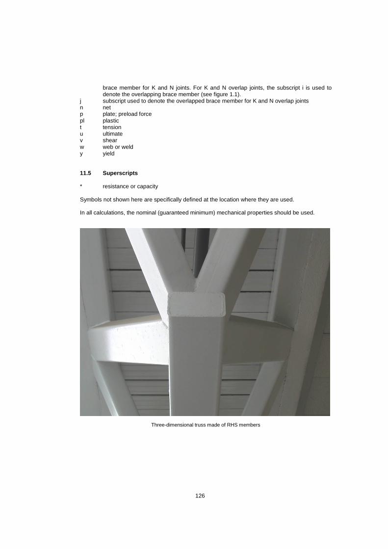
126

brace member for K and N joints. For K and N overlap joints, the subscript i is used to denote the overlapping brace member (see figure 1.1).

j subscript used to denote the overlapped brace member for K and N overlap joints n net p plate; preload force pl plastic t tension u ultimate v shear w web or weld y yield 11.5 Superscripts * resistance or capacity Symbols not shown here are specifically defined at the location where they are used. In all calculations, the nominal (guaranteed minimum) mechanical properties should be used.

Three-dimensional truss made of RHS members

127

12 References AISC, 2005: Specification for structural steel buildings. ANSI/AISC 360-05, American Institute of Steel Construction, Chicago, Ill., USA. ASTM, 2007a: Standard specification for pipe, steel, black and hot-dipped, zinc-coated, welded and seamless. ASTM A53/A53M-07, ASTM International, West Conshohocken, Pa., USA. ASTM, 2007b: Standard specification for cold-formed welded and seamless carbon steel structural tubing in rounds and shapes. ASTM A500/A500M-07, ASTM International, West Conshohocken, Pa., USA. ASTM, 2007c: Standard specification for hot-formed welded and seamless carbon steel structural tubing. ASTM A501-07, ASTM International, West Conshohocken, Pa., USA. AWS, 2008: Structural welding code – Steel. 21st Edition, AWS D1.1/D1.1M:2008, American Welding Society, Miami, Fl, USA. Bauer, D., and Redwood, R.G., 1988: Triangular truss joints using rectangular tubes. Journal of Structural Engineering, American Society of Civil Engineers, Vol. 114, No. 2, pp. 408-424. Birkemoe, P.C., and Packer, J.A., 1986: Ultimate strength design of bolted tubular tension connections. Proceedings Conference on Steel Structures – Recent Research Advances and their Applications to Design, Budva, Yugoslavia, pp. 153-168. Björk, T., Marquis, G., Kemppainen, R., and Ilvonen, R., 2003 : The capacity of cold-formed rectangular hollow section K gap joints. Proceedings 10th International Symposium on Tubular Structures, Madrid, Spain, Tubular Structures X, Swets & Zeitlinger, Lisse, The Netherlands, pp. 227-234. Bouwman, L.P., 1979: Fatigue of bolted connections and bolts loaded in tension. Stevin Report 6-79-9, Delft University of Technology, Delft, The Netherlands. Brockenbough, R.L., 1972: Strength of square tube connections under combined loads. Journal of the Structural Division, American Society of Civil Engineers, Vol. 98, No. ST12, pp. 2753-2768. Cao, J.J., Packer, J.A., and Kosteski, N., 1998a: Design guidelines for longitudinal plate to HSS connections. Journal of Structural Engineering, American Society of Civil Engineers, Vol. 124, No. 7, pp. 784-791. Cao, J.J., Packer, J.A., and Yang, G.J., 1998b: Yield line analysis of RHS connections with axial loads. Journal of Constructional Steel Research, Vol. 48, No. 1, pp. 1-25. Caravaggio, A., 1988: Tests on steel roof joints for Toronto SkyDome. M.A.Sc. Thesis, University of Toronto, Canada. CEN, 2005a: Eurocode 3: Design of steel structures − Part 1-1: General rules and rules for buildings. EN 1993-1-1:2005(E), European Committee for Standardization, Brussels, Belgium. CEN, 2005b: Eurocode 3: Design of steel structures − Part 1-8: Design of joints. EN 1993-1-8:2005(E), European Committee for Standardization, Brussels, Belgium. CEN, 2006a: Hot-finished structural hollow sections of non-alloy and fine grain steels – Part 2: Tolerances, dimensions and sectional properties. EN 10210-2:2006(E), European Committee for Standardization, Brussels, Belgium.

128

CEN, 2006b: Cold-formed welded structural hollow sections of non-alloy and fine grain steels – Part 2: Tolerances, dimensions and sectional properties. EN 10219-2:2006(E), European Committee for Standardization, Brussels, Belgium. Chen, Y., Liu, D.K., and Wardenier, J., 2005: Design recommendations for RHS-K joints with 100% overlap. Proceedings 15th International Offshore and Polar Engineering Conference, Seoul, Korea, Vol. IV, pp. 300-307. CIDECT, 1984: Construction with hollow steel sections. British Steel Plc., Corby, Northants, UK, ISBN 0-9510062-0-7. Coutie, M.G., Davies, G., Bettison, M., and Platt, J., 1983: Development of recommendations for the design of welded joints between steel structural hollow sections or between steel structural hollow sections and H sections. Final Report, Part 3: Three dimensional joints. Report on ECSC Contract 7210.5A1814, University of Nottingham, UK. Coutie, M.G., Davies, G., Philiastides, A., and Yeomans, N., 1987: Testing of full-scale lattice girders fabricated with RHS members. Conference on Structural Assessment Based on Full and Large-Scale Testing, Building Research Station, Watford, UK. CSA, 2004: General requirements for rolled or welded structural quality steel/structural quality steel. CAN/CSA G40.20-04/G40.21-04, Canadian Standards Association, Toronto, Canada. CSA, 2009: Design of steel structures. CSA-S16-09, Canadian Standards Association, Toronto, Canada. Cute, D., Camo, S., and Rumpf, J.L., 1968: Welded connections for square and rectangular structural steel tubing. Research Report No. 292-10, Drexel Institute of Technology, Philadelphia, Pa, USA. Czechowski, A., Gasparski, T., Zycinski, J., and Brodka, J., 1984: Investigation into the static behaviour and strength of lattice girders made of RHS. International Institute of Welding, IIW Doc. XV-562-84, Poland. Davies, G., and Packer, J.A., 1982: Predicting the strength of branch plate-RHS connections for punching shear. Canadian Journal of Civil Engineering, Vol. 9, pp. 458-467. Davies, G., and Panjeh Shahi, E., 1984: Tee joints in rectangular hollow sections (RHS) under combined axial loading and bending. Proceedings 7th International Symposium on Steel Structures, Gdansk, Poland. Davies, G., and Morita, K., 1991: Three dimensional cross joints under combined axial branch loading. Proceedings 4th International Symposium on Tubular Structures, Delft, The Netherlands, Delft University Press, Delft, The Netherlands, pp. 324-333. Davies, G., and Kelly, R.B., 1995: Bird beak joints in square hollow sections – A finite element investigation. Proceedings 4th Pacific Structural Steel Conference, Singapore. Davies, G., Owen, J.S., and Kelly, R.B., 1996: Bird beak T-joints in square hollow sections – A finite element investigation. Proceedings 6th International Offshore and Polar Engineering Conference, Los Angeles, USA, Vol. IV, pp. 22-27. Davies, G., Owen, J.S., and Kelly, R.B., 2001: The effect of purlin loads on the capacity of overlapped bird-beak K joints. Proceedings 9th International Symposium on Tubular Structures, Düsseldorf, Germany, Tubular Structures IX, Swets & Zeitlinger, Lisse, The Netherlands, pp. 229-238.

129

Driver, R.G., Grondin, G.Y., and Kulak, G.L., 2006: Unified block shear equation for achieving consistent reliability. Journal of Constructional Steel Research, Vol. 62, No. 3, pp. 210-222. Duff, G., 1963: Joint behaviour of a welded beam-column connection in rectangular hollow sections. Ph.D. Thesis, The College of Aeronautics, Cranfield, UK. Dutta, D., and Würker, K., 1988: Handbuch Hohlprofile in Stahlkonstruktionen. Verlag TÜV Rheinland GmbH, Köln, Germany. Dutta, D., Wardenier, J., Yeomans, N., Sakae, K., Bucak, Ö., and Packer, J.A., 1998: Design guide for fabrication, assembly and erection of hollow section structures. CIDECT series ‘Construction with hollow sections’ No. 7, TÜV-Verlag, Köln, Germany. Dutta, D., 2002: Structures with hollow sections. Ernst & Sohn, Verlag, Berlin, Germany. Eekhout, M., 1996: Tubular structures in architecture. CIDECT and Delft University of Technology, Delft, The Netherlands. Fleischer, O., and Puthli, R., 2008: Extending existing design rules in EN 1993-1-8 (2005) for gapped RHS K-joints for maximum chord slenderness (b0/t0) of 35 to 50 and gap size g to as low as 4t0. Proceedings 12th International Symposium on Tubular Structures, Shanghai, China, Tubular Structures XII, Taylor & Francis Group, London, UK, pp. 293-301. Frater, G.S., and Packer, J.A., 1990: Design of fillet weldments for hollow structural section trusses. CIDECT Report No. 5AN/2-9017, University of Toronto, Canada. Frater, G.S., 1991: Performance of welded rectangular hollow structural section trusses. Ph.D. Thesis, University of Toronto, Canada. Galambos, T.V. (Ed.), 1998: Guide to stability design criteria for metal structures, 5th Edition, Structural Stability Research Council, John WiIey & Sons, New York, USA. Ghosh, A., and Morris, G., 1981: Behaviour of tubular steel trusses with cropped webs. Canadian Journal of Civil Engineering, Vol. 8, No. 1, pp. 51-58. Grundy, P., and Foo, E.K.J., 1991: Performance of flattened tube connections. Proceedings 4th International Symposium on Tubular Structures, Delft, The Netherlands, Delft University Press, Delft, The Netherlands, pp. 251-258. Horne, M.R., and Morris, L.J., 1985: Plastic design of low-rise frames. Collins, London, UK. IIW, 1989: Design recommendations for hollow section joints – Predominantly statically loaded. 2nd

Edition, International Institute of Welding, Commission XV, IIW Doc. XV-701-89. IIW, 2009: Static design procedure for welded hollow section joints – Recommendations. 3rd Edition, International Institute of Welding, Commission XV, IIW Doc. XV-1329-09. Ishida, K., Ono, T., and Iwata, M., 1993: Ultimate strength formula for joints of new truss system using rectangular hollow sections. Proceedings 5th International Symposium on Tubular Structures, Nottingham, UK, Tubular Structures V, E & FN Spon, London, UK, pp. 511-518. Kanatani, H., Fujiwara, K., Tabuchi, M., and Kamba, T., 1980: Bending tests on T-joints of RHS chord and RHS or H-shape branch, CIDECT Report 5AF-80/15. Kanatani, H., Kamba, T., and Tabuchi, M., 1986: Effect of the local deformation of the joints on RHS Vierendeel trusses. Proceedings International Meeting on Safety Criteria in Design of Tubular Structures, Tokyo, Japan, pp. 127-137.

130

Karcher, D., and Puthli, R.S., 2001: The static design of stiffened and unstiffened CHS L-joints. Proceedings 9th lnternational Symposium on Tubular Structures, Düsseldorf, Germany, Tubular Structures IX, Swets & Zeitlinger, Lisse, The Netherlands, pp. 221-228. Kato, B., and Mukai, A., 1985: Bolted tension flanges square hollow section members. Supplement in 1985: Bolted at two sides of flange. CIDECT Program 8B Report, University of Tokyo, Japan. Kitipornchai, S., and Traves, W.H., 1989: Welded tee end connections for circular hollow tubes. Journal of Structural Engineering, American Society of Civil Engineers, Vol. 115, No. 12, pp. 3155-3170. Koning, C.H.M. de, and Wardenier, J., 1984: The static strength of welded joints between structural hollow sections or between structural hollow sections and H-sections. Part 2: Joints between rectangular hollow sections. Stevin Report 6-84-19, Delft University of Technology, Delft, The Netherlands. Korol, R.M., El-Zanaty, M., and Brady, F.J., 1977: Unequal width connections of square hollow sections in Vierendeel trusses. Canadian Journal of Civil Engineering, Vol. 4, pp. 190-201. Korol, R.M., and Mansour, M.H., 1979: Theoretical analysis of haunch-reinforced T-joints in square hollow sections. Canadian Journal of Civil Engineering, Vol. 6, No. 4, pp. 601-609. Korol, R.M., and Chidiac, M.A., 1980: K-joints of double-chord square hollow-sections. Canadian Journal of Civil Engineering, Vol. 7, No. 3, pp. 523-539. Korol, R.M., and Mirza, F.A., 1982: Finite element analysis of RHS T-joints. Journal of the Structural Division, American Society of Civil Engineers, Vol. 108, No. ST9, pp. 2081-2098. Korol, R.M., Mitri, H.S., and Mirza, F.A., 1982: Plate reinforced square hollow section T-joints of unequal width. Canadian Journal of Civil Engineering, Vol. 9, No. 2, pp. 143-148. Korol, R.M., 1983: The behaviour of HSS double chord Warren trusses and aspects of design. Canadian Symposium on HSS, CIDECT, Lecture tour to Canadian cities. Korol, R.M., Mirza, F.A., and Chiu, E.T.-C., 1983: An experimental investigation of double-chord HSS trusses. Canadian Journal of Civil Engineering, Vol. 10, No. 2, pp. 248-260. Korol, R.M., and Mitri, H.S., 1985: Strength analysis of RHS double chord joints with separated chords. Canadian Journal of Civil Engineering, Vol. 12, No. 2, pp. 370-381. Kosteski, N., 2001: Branch plate to rectangular hollow section member connections. Ph.D. Thesis, University of Toronto, Toronto, Canada. Kosteski, N., and Packer, J.A., 2003a: Welded tee-to-HSS connections. Journal of Structural Engineering, American Society of Civil Engineers, Vol. 129, No. 2, pp. 151-159. Kosteski, N., and Packer, J.A., 2003b: Longitudinal plate and through plate-to-HSS welded connections. Journal of Structural Engineering, American Society of Civil Engineers, Vol. 129, No. 4, pp. 478-486. Kosteski, N., Packer, J.A., and Puthli, R.S., 2005: Notch toughness of internationally produced hollow structural sections. Journal of Structural Engineering, American Society of Civil Engineers, Vol. 131, No. 2, pp. 279-286. Kurobane, Y., Packer, J.A., Wardenier, J., and Yeomans, N., 2004: Design guide for structural hollow section column connections. CIDECT series ‘Construction with hollow sections’ No. 9, TÜV-Verlag, Köln, Germany.

131

Lau, B.L., Morris, G.A., and Pinkney, R.B., 1985: Testing of Warren-type cropped-web tubular truss joints. Canadian Society for Civil Engineering Annual Conference, Saskatoon, Canada. Lazar, B.E., and Fang, P.J., 1971: T-type moment connections between rectangular tubular sections. Research Report, Sir George Williams University, Montreal, Canada. Liu, D.K., and Wardenier, J., 2001a: Multiplanar influence on the strength of RHS multiplanar gap KK-joints. Proceedings 9th International Symposium on Tubular Structures, Düsseldorf, Germany, Tubular Structures IX, Swets & Zeitlinger, Lisse, The Netherlands, pp. 203-212. Liu, D.K., and Wardenier, J., 2001b: The strength of multiplanar gap KK joints of rectangular hollow sections under axial loading. Proceedings 11th International Offshore and Polar Engineering Conference, Stavanger, Norway, Vol. IV, pp. 15-22. Liu, D.K., and Wardenier, J., 2002: The strength of multiplanar overlap KK-joints of rectangular hollow sections under axial loading. Proceedings 12th International Offshore and Polar Engineering Conference, Kitakyushu, Japan, Vol. IV, pp. 34-40. Liu, D.K., and Wardenier, J., 2003: The strength of multiplanar KK-joints of square hollow sections. Proceedings 10th International Symposium on Tubular Structures, Madrid, Spain, Tubular Structures X, Swets & Zeitlinger, Lisse, The Netherlands, pp. 197-205. Liu, D.K., and Wardenier, J., 2004: Effect of the yield strength on the static strength of uniplanar K-joints in RHS (steel grades S460, S355 and S235). IIW Doc. XV-E-04-293, Delft University of Technology, Delft, The Netherlands. Liu, D.K., Chen, Y., and Wardenier, J., 2005: Design recommendations for RHS-K joints with 50% overlap. Proceedings 15th International Offshore and Polar Engineering Conference, Seoul, Korea, Vol. IV, pp. 308-315. Lu, L.H., Winkel, G.D. de, Yu, Y., and Wardenier, J., 1994: Deformation limit for the ultimate strength of hollow section joints. Proceedings 6th International Symposium on Tubular Structures, Melbourne, Australia, Tubular Structures VI, Balkema, Rotterdam, The Netherlands, pp. 341-347. Lu, L.H., 1997: The static strength of I-beam to rectangular hollow section column connections. Ph.D. Thesis, Delft University Press, Delft, The Netherlands. Luft, R.T., Korol, R.M., and Huitema, H.A.P., 1991: An economic comparison of single chord and double chord RHS Warren trusses. Proceedings 4th International Symposium on Tubular Structures, Delft, The Netherlands, Delft University Press, Delft, The Netherlands, pp. 11-20. Mang, F., 1980: Investigation of standard bolted flange connections for circular and rectangular hollow sections. CIDECT Report 8A-81/7-E, University of Karlsruhe, Germany. Mang, F., Steidl, G., and Bucak, Ö., 1980: Design of welded lattice joints and moment resisting knee joints made of hollow sections. International Insitute of Welding, IIW Doc. XV-463-80, University of Karlsruhe, Germany. Mang, F., Bucak, Ö., and Wolfmuller, F., 1983: The development of recommendations for the design of welded joints between steel structural hollow sections (T- and X-type joints). University of Karlsruhe, Germany, Final Report on ECSC Agreement 7210 SA/l 09 and CIDECT Program 5AD. Martinez-Saucedo, G., and Packer, J.A., 2006: Slotted end connections to hollow sections. CIDECT Final Report 8G-10/4, University of Toronto, Toronto, Canada. Mehrotra, B.L., and Redwood, R.G., 1970: Load transfer through connections between box sections. Canadian Engineering Institute, C-70-BR and ST 10, Canada.

132

Mehrotra, B.L., and Govil, A.K., 1972: Shear lag analysis of rectangular full-width tube connections. Journal of the Structural Division, American Society of Civil Engineers, Vol. 98, No. ST1, pp. 287-305. Morris, G.A., 1985: Tubular steel trusses with cropped webs. Journal of Structural Engineering, American Society of Civil Engineers, Vol. 111, No. 6, pp. 1338-1357. Morris, G.A., and Packer, J.A., 1988: Yield line analysis of cropped-web Warren truss joints. Journal of Structural Engineering, American Society of Civil Engineers, Vol. 114, No. 10, pp. 2210-2224. Mouty, J. (Ed.), 1981: Effective lengths of lattice girder members. CIDECT Monograph No. 4, CIDECT. Ono, T., Iwata, M., and Ishida, K., 1991: An experimental study on joints of new truss system using rectangular hollow sections. Proceedings 4th International Symposium on Tubular Structures, Delft, The Netherlands, Delft University Press, Delft, The Netherlands, pp. 344-353. Ono, T., Iwata, M., and Ishida, K., 1993: Local failure of joints of new truss system using rectangular hollow sections subjected to in-plane bending moment. Proceedings 5th International Symposium on Tubular Structures, Nottingham, UK, Tubular Structures V, E & FN Spon, London, UK, pp. 503-510. Ono, T., Iwata, M., and Ishida, K., 1994: Local failure of joints of new truss system using rectangular hollow sections subjected to out-of-plane bending moment. Proceedings 6th International Symposium on Tubular Structures, Melbourne, Australia, Tubular Structures VI, Balkema, Rotterdam, The Netherlands, pp. 441-448. Owen, J.S., Davies, G., and Kelly, R.B., 1996: A comparison of the behaviour of RHS bird beak T-joints with normal RHS and CHS systems. Proceedings 7th International Symposium on Tubular Structures, Miskolc, Hungary, Tubular Structures VII, Balkema, Rotterdam, The Netherlands, pp. 173-180. Packer, J.A., and Haleem, A.S., 1981: Ultimate strength formulae for statically loaded welded HSS joints in lattice girders with RHS chords. Proceedings Canadian Society for Civil Engineering Annual Conference, Fredericton, Canada, Vol. 1, pp. 331-343. Packer, J.A., Bruno, L., and Birkemoe, P.C., 1989: Limit analysis of bolted RHS flange plate joints. Journal of Structural Engineering, American Society of Civil Engineers, Vol. 115, No. 9, pp. 2226-2242. Packer, J.A., 1991: Cranked-chord HSS connections. Journal of Structural Engineering, American Society of Civil Engineers, Vol. 117, No. 8, pp. 2224-2240. Packer, J.A., and Fear, C.E., 1991: Concrete-filled rectangular hollow section X and T connections. Proceedings 4th International Symposium on Tubular Structures, Delft, The Netherlands, Delft University Press, Delft, The Netherlands, pp. 382-391. Packer, J.A., and Wardenier, J., 1992: Design rules for welds in RHS K, T, Y and X connections. IIW International Conference on Engineering Design in Welded Construction, Madrid, Spain, pp. 113-120. Packer, J.A., Wardenier, J., Kurobane, Y., Dutta, D., and Yeomans, N., 1992: Design guide for rectangular hollow section (RHS) joints under predominantly static loading. 1st Edition, CIDECT series ‘Construction with hollow sections’ No. 3, TÜV-Verlag, Köln, Germany. Packer, J.A., 1995: Concrete-filled HSS connections. Journal of Structural Engineering, American Society of Civil Engineers, Vol. 121, No. 3, pp. 458-467.

133

Packer, J.A., and Henderson, J.E., 1997: Hollow structural section connections and trusses – A design guide. 2nd Edition, Canadian Institute of Steel Construction, Toronto, Canada. Packer, J.A., 2007: Design with hollow structural sections – A report on recent developments in the USA. Proceedings 5th International Conference on Advances in Steel Structures, Singapore, Vol. II, pp. 228-237. Packer, J.A., Sherman, D.R., and Lecce, M., 2009: HSS connections. Steel Design Guide No. 24, American Institute of Steel Construction, Chicago, Ill., USA. Papanikolas, P.C., Nowak, J.A., and Kulak, G.L., 1990: Flexible flattened HSS connections. Report by Northern Steel Inc., Edmonton, Canada. Philiastides, A., 1988: Fully overlapped rolled hollow section welded joints in trusses. Ph.D. Thesis, University of Nottingham, UK. Qian, X.D., Wardenier, J., and Choo, Y.S., 2007: A uniform approach for the design of CHS 100% overlap joints. Proceedings 5th International Conference on Advances in Steel Structures, Singapore, Vol. II, pp. 172-182. Redwood, R.G., 1965: The behaviour of joints between rectangular hollow structural members. Civil Engineering and Public Works Review, Canada, pp. 1463-1469. Rondal, J., Würker, K.-G., Dutta, D., Wardenier, J., and Yeomans, N., 1996: Structural stability of hollow sections. 2nd Printing, CIDECT series ‘Construction with hollow sections’ No. 2, TÜV-Verlag, Köln, Germany. Sedlacek, G., Wardenier, J., Dutta, D., and Grotmann, D., 1991: Evaluation of test results on hollow section lattice girder connections. Background Report to Eurocode 3 ‘Common unified rules for steel structures’, Document 5.07, Eurocode 3 Editorial Group. Sedlacek, G., Völling, B., Pak, D., and Feldmann, M., 2006: Local buckling behaviour of cold-formed RHS made from S1100. Proceedings 11th International Symposium on Tubular Structures, Quebec City, Canada, Tubular Structures XI, Taylor & Francis Group, London, UK, pp. 147-152. Sherman, D.R., 1995: Simple framing connections to HSS columns. Proceedings National Steel Construction Conference, San Antonio, Tex., USA, American Institute of Steel Construction, Chicago, Ill., USA, pp. 30.1-30.16. Sherman, D.R., 1996: Designing with structural tubing. Engineering Journal, American Institute of Steel Construction, Vol. 33, No. 3, pp. 101-109. Shinouda, M.R., 1967: Stiffened tubular joints. Ph.D. Thesis, University of Sheffield, UK. Standards Australia, 1991: Structural steel hollow sections. Australian Standard AS 1163, Standards Australia, Sydney, Australia. Staples, C.J.L., and Harrison, C.C., undated: Test results of 24 right-angled branches fabricated from rectangular hollow sections. University of Manchester Institute of Science and Technology (UMIST) Report, Manchester, UK. Stelco, 1981: Hollow structural sections – Design manual for connections. 2nd Edition, Stelco Inc., Hamilton, Canada. Struik, J.H.A., and Back, J. de, 1969: Tests on bolted T-stubs with respect to a bolted beam-to-column connection. Stevin Report 6-69-13, Delft University of Technology, Delft, The Netherlands.

134

Szlendak, J., and Brodka, J., 1985: Strengthening of T moment of RHS joints. Proceedings Institution of Civil Engineers, Part 2, Vol. 79, pp. 717-727. Szlendak, J., 1986: Interaction curves for M-N loaded T RHS joints. Proceedings International Meeting on Safety Criteria in Design of Tubular Structures, Tokyo, Japan, pp. 169-174. Szlendak, J., and Brodka, J., 1986a: Design of strengthen frame RHS joints. Proceedings International Meeting on Safety Criteria in Design of Tubular Structures, Tokyo, Japan, pp. 159-168. Szlendak, J., and Brodka, J., 1986b: Reply to discussion by J.A. Packer on paper “Strengthening of T moment of RHS joints”. Proceedings Institution of Civil Engineers, Part 2, Vol. 81, pp. 721-725. Szlendak, J., 1991: Beam-column welded RHS connections. Journal of Thin-Walled Structures, Vol. 12, pp. 63-80. Thornton, W.A., 1984: Bracing connections for heavy construction. Engineering Journal, American Institute of Steel Construction, Vol. 21, Third Quarter, pp. 139-148. Wardenier, J., 1972: Investigation on Vierendeel joints; Determination of M-Φ and P-δ characteristics and the fatigue behaviour. Stevin Report 6-72-11, Delft University of Technology, Delft, The Netherlands, (in Dutch). Wardenier, J., and Stark, J.W.B., 1978: The static strength of welded lattice girder joints in structural hollow sections: Parts 1-10. CIDECT Final Report 5Q-78/4, Delft University of Technology, Delft, The Netherlands. Wardenier, J., Davies, G., and Stolle, P., 1981: The effective width of branch plate to RHS chord connections in cross joints. Stevin Report 6-81-6, Delft University of Technology, Delft, The Netherlands. Wardenier, J., 1982: Hollow section joints. Delft University Press, Delft, The Netherlands. Wardenier, J., Kurobane, Y., Packer, J.A., Dutta, D., and Yeomans, N., 1991: Design guide for circular hollow section (CHS) joints under predominantly static loading. 1st Edition, CIDECT series ‘Construction with hollow sections’ No. 1, TÜV-Verlag, Köln, Germany. Wardenier, J., 2002: Hollow sections in structural applications. Bouwen met Staal, Zoetermeer, The Netherlands. Wardenier, J., 2007: A uniform effective width approach for the design of CHS overlap joints. Proceedings 5th International Conference on Advances in Steel Structures, Singapore, Vol. II, pp. 155-165. Wardenier, J., Vegte, G.J. van der, and Liu, D.K., 2007a: Chord stress function for rectangular hollow section X and T joints. Proceedings 17th International Offshore and Polar Engineering Conference, Lisbon, Portugal, Vol. IV, pp. 3363-3370. Wardenier, J., Vegte, G.J. van der, and Liu, D.K., 2007b: Chord stress functions for K gap joints of rectangular hollow sections. International Journal of Offshore and Polar Engineering, ISOPE, Vol. 17, No. 3, pp. 225-232. Wardenier, J., Kurobane, Y., Packer, J.A., Vegte, G.J. van der, and Zhao, X.-L., 2008: Design guide for circular hollow section (CHS) joints under predominantly static loading. 2nd Edition, CIDECT series ‘Construction with hollow sections’ No. 1, CIDECT, Geneva, Switzerland. Whitmore, R.E., 1952: Experimental investigation of stresses in gusset plates. Bulletin 16, University of Tennessee Engineering Experiment Station, USA.

135

Willibald, S., Puthli, R.S., and Packer, J.A., 2001: Experimentelle Studie zu geschraubten Kopfplatten-Verbindungen für Quadrathohlprofile. Stahlbau, Vol. 70, No. 3, pp. 183-192, (in German). Willibald, S., Packer, J.A., and Puthli, R.S., 2002: Experimental study of bolted HSS flange-plate connections in axial tension. Journal of Structural Engineering, American Society of Civil Engineers, Vol. 128, No. 3, pp. 328-336. Willibald, S., Packer, J.A., and Puthli, R.S., 2003a: Design recommendations for bolted rectangular HSS flange-plate connections in axial tension. Engineering Journal, American Institute of Steel Construction, Vol. 40, First Quarter, pp. 15-24. Willibald, S., Packer, J.A., and Puthli, R.S., 2003b: Investigation on hidden joint connections under tensile loading. Proceedings 10th International Symposium on Tubular Structures, Madrid, Spain, Tubular Structures X, Swets & Zeitlinger, Lisse, The Netherlands, pp. 217-225. Yeomans, N.F., and Giddings, T.W., 1988: The design of full width joints in RHS Vierendeel girders. Report No. 800/0/72, British Steel Plc., Corby, UK. Yu, Y., 1997: The static strength of uniplanar and multiplanar connections in rectangular hollow sections. Ph.D. Thesis, Delft University Press, Delft, The Netherlands. Zhao, X.-L., Wardenier, J., Packer, J.A., and Vegte, G.J. van der, 2008: New IIW (2008) static design recommendations for hollow section joints, Proceedings 12th International Symposium on Tubular Structures, Shanghai, China, Tubular Structures XII, Taylor & Francis Group, London, UK, pp. 261-269.

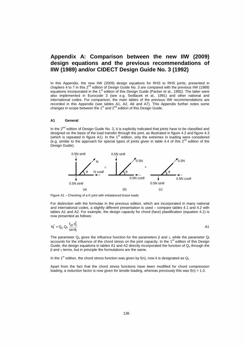
136

Appendix A: Comparison between the new IIW (2009) design equations and the previous recommendations o f IIW (1989) and/or CIDECT Design Guide No. 3 (1992) In this Appendix, the new IIW (2009) design equations for RHS to RHS joints, presented in chapters 4 to 7 in this 2nd edition of Design Guide No. 3 are compared with the previous IIW (1989) equations incorporated in the 1st edition of this Design Guide (Packer et al., 1992). The latter were also implemented in Eurocode 3 (see e.g. Sedlacek et al., 1991) and other national and international codes. For comparison, the main tables of the previous IIW recommendations are recorded in this Appendix (see tables A1, A2, A6 and A7). This Appendix further notes some changes in scope between the 1st and 2nd edition of this Design Guide. A1 General In the 2nd edition of Design Guide No. 3, it is explicitly indicated that joints have to be classified and designed on the basis of the load transfer through the joint, as illustrated in figure 4.2 and figure 4.3 (which is repeated in figure A1). In the 1st edition, only the extremes in loading were considered (e.g. similar to the approach for special types of joints given in table 4.4 of this 2nd edition of the Design Guide).

0.5N sinθ

0.5N sinθ

θ

N

N cosθ=

0.5N sinθ

θ

0.5N

0.5N cosθ0.5N sinθ

θ+

0.5N

0.5N cosθ

(a) (b) (c)

Figure A1 – Checking of a K joint with imbalanced brace loads For distinction with the formulae in the previous edition, which are incorporated in many national and international codes, a slightly different presentation is used – compare tables 4.1 and 4.2 with tables A1 and A2. For example, the design capacity for chord (face) plastification (equation 4.1) is now presented as follows:

i

20 y0

fu*i

θ sin

tf Q QN = A1

The parameter Qu gives the influence function for the parameters β and γ, while the parameter Qf accounts for the influence of the chord stress on the joint capacity. In the 1st edition of this Design Guide, the design equations in tables A1 and A2 directly incorporated the function of Qu through the β and γ terms, but in principle the formulations are the same. In the 1st edition, the chord stress function was given by f(n), now it is designated as Qf. Apart from the fact that the chord stress functions have been modified for chord compression loading, a reduction factor is now given for tensile loading, whereas previously this was f(n) = 1.0.

137

Table A1 – Design resistance of uniplanar RHS braces or CHS braces to RHS chord joints according to IIW (1989) and the 1st edition of Design Guide No. 3 (Packer et al., 1992)

Type of joint Factored joint resistance (i = 1,2)

T, Y and X joints β ≤ 0.85 basis: chord face plastification

t 0 t 1

d 1

h 1

b 1

h 0

b 0

N 1

θ 1

( ) ( ) f(n) -14θsin

2θsin β-1

tfN 5.0

1 1

2 0 y0*

1

β+η=

β = 1.0 basis: chord side wall failure (*)

For 0.85 < β ≤ 1.0, use linear interpolation between chord face plastification and chord side wall failure criteria

10tθsin

2hθsintf

N 01

1

1

0 k*1

+=

β > 0.85 basis: local yielding of brace

[ ] b2t42htfN e11 1 y1*1 +−=

0.85 ≤ β ≤ 1-1/γ basis: chord punching shear

2bθsin

2h

θsin 3

tfN pe,

1

1

1

0 y0*1

+=

K and N gap joints basis: chord face plastification

g

d 1

θ 1 θ 2 t 0

t 2 2 1

+e

0

h 1

b 1

d 2h 2

b 2

h 0

b 0t 1

N 0

N 1 N 2

1,2) (i f(n) b 4

hhbbθsin

tf9.8N 0.5

0

2 1 2 1

i

2 0 y0*

i =γ

+++=

basis: chord shear

θsin 3

AfN

i

v y0*i =

Also ( ) ( ) 2 pl,0gap,0 y0 vy0 v0

*0,gapgap,0 V/V1fAfAANN −+−=≤

basis: local yielding of brace

[ ] bbt42htfN eiii i yi*i ++−=

β ≤ 1-1/γ basis: chord punching shear

bbθsin

2h

θsin 3

tfN pe,i

i

i

i

0 y0*i

++=

K and N overlap joints Similar to joints of SHS (table A2) CHS braces Multiply formulae by π/4 and replace b1,2 and h1,2 by d1,2

Functions

tension: fk = fy0 compression: fk = fkn (T and Y joints) fk = 0.8 sin θ1 fkn (X joints)

fkn = buckling stress according to the relevant steelwork specification, using a column

slenderness ratio (KL/r) of ( ) ( ) θ1/sin 2/th3.46 0.5 1 00 −

on)(compressi 1.0but

0 n for n0.4

1.3 f(n)

(tension) 0n for 1.0f(n)

≤

<β

+=

≥=

3

AfV v 0y

pl,0 = )t3( /)g4(1

120

2+=α

For SHS and RHS braces: ( ) 0 00v tb2hA α+=

For CHS braces: 0 0v t2hA =

ii i yi

0 y0

00e b but b

tf

tf

/tb10

b ≤= ii00

pe, b but b/tb

10b ≤= ii

i yi

j yj

jjove, b but b

tf

tf

/tb10

b ≤=

(*) For X joints with angles θ1 < 90°, the chord side walls must be checked for shear

138

Table A1a – Range of validity of table A1

Type of joint Joint parameters (i = 1 or 2, j = overlapped brace ) (*)

bi/b0 hi/b0

bi/ti, hi/ti, di/ti hi/bi

b0/t0 h0/t0

Gap/overlap bi/bj ti/tj

Eccentricity Compression Tension

T, Y and X joints ≥ 0.25

y1fE

25.1≤

≤ 35 ≤ 35 2

bh

5.0i

i ≤≤

≤ 35

K and N gap joints 0

0

tb

01.01.0 +≥

β ≥ 0.35

≤ 35 ( ) ( )β−≤≤β− 15.1

bg

15.0 0

(**)

g ≥ t1 + t2 25.0

he

55.00

≤≤−

K and N overlap joints ≥ 0.25

y1fE

1.1≤ ≤ 40

25% ≤ Ov ≤ 100%

75.0bb

,0.1tt

j

i

j

i ≥≤

CHS braces (web members)

8.0bd

4.00

i ≤≤ y1f

E5.1≤ ≤ 50 Limitations as above for di = bi

(*) fyi and fyj ≤ 355 N/mm2, fyi (or fyj)/fui ≤ 0.8

(**) If > 0b

g the larger of 1.5(1-β) and (t1 + t2), treat as a T or Y joint

139

Table A2 – Design resistance of uniplanar SHS braces or CHS braces to SHS chord joints according to IIW (1989) and the 1st edition of Design Guide No. 3 (Packer et al., 1992)

Type of joint Factored joint resistance (i = 1,2)

T, Y and X joints β ≤ 0.85 basis: chord face plastification

t 0 t 1

d 1

h 1

b 1

h 0

b 0

N 1

θ 1

( ) ( ) f(n) -14θsin

2θsin -1

tfN 5.0

1

1

2 0 y0*

1

β+β

β=

K and N gap joints β ≤ 1.0 basis: chord face plastification

g

d 1

θ 1 θ 2 t 0

t 2 2 1

+e

0

h 1

b 1

d 2h 2

b 2

h 0

b 0

t 1

N 0

N 1 N 2

1,2) (i f(n) b 2bb

θsin

tf9.8N 0.5

0

2 1

i

2 0 y0*

i =γ

+=

K and N overlap joints (*) 25% ≤ Ov < 50% basis: local yielding of overlapping brace

( ) bbt42h 50Ov

tfN ove,eii i yi*i

++−

=

50% ≤ Ov < 80% basis: local yielding of overlapping brace

[ ] bbt42htfN ove,eii i yi*i ++−=

Ov ≥ 80% basis: local yielding of overlapping brace

[ ] bbt42htfN ove,iii i yi*i ++−=

CHS braces Multiply by π/4 and replace b1,2 and h1,2 by d1,2

Functions

1.0f(n) but on)(compressi 0 n for n0.4

1.3 f(n)

(tension) 0n for 1.0f(n)

≤<β

+=

≥=

ii i yi

0 y0

00e b but b

tf

tf

/tb10

b ≤= ii i yi

j yj

jjove, b but b

tf

tf

/tb10

b ≤=

(*) Only the overlapping brace need be checked for local yielding. However, the efficiency (the factored joint resistance divided by the yield capacity of the brace) of the overlapped brace should not exceed that of the overlapping brace.

d i

d 0 θ i θ j t 0

t j j i

-e 0

h i

b i

d jh j

b j

h 0

b 0

t i

N i N j

N 0

p

q

140

Table A2a – Range of validity of table A2

Type of joint Joint parameters (i = 1 or 2; j = overlapped brace) (*)

bi/b0 bi/ti

b0/t0 (b1+b2)/2bi

bi/bj ti/tj Gap/overlap Eccentricity

Compression Tension

T, Y and X joints

85.025.0 ≤β≤

(**) y1f

E25.1≤

≤ 35

≤ 35

35tb

(**) 100

0 ≤≤

K and N gap joints

0

0

tb

01.01.0 +≥

β ≥ 0.35

35tb

(**) 150

0 ≤≤ 2

bb77.0b 21

i+≥ (**)

( ) ( )β−≤≤β− 15.1bg

15.0 0

g ≥ t1 + t2 (***)

25.0he

55.00

≤≤−

K and N overlap joints ≥ 0.25

y1fE

1.1≤ 40tb

0

0 ≤

75.0bb

0.1tt

j

i

j

i

≥

≤

25% ≤ Ov ≤ 100%

CHS braces 8.0bd

4.00

i ≤≤ y11

1

fE

5.1td ≤ 50

td

2

2 ≤ Limitations as above for di = bi

(*) fyi and fyj ≤ 355 N/mm2, fyi (or fyj)/fui ≤ 0.8

(**) Outside this range of validity, other criteria may be governing; e.g. chord punching shear, local yielding of the (overlapping) brace, chord side wall failure, chord shear or local buckling. If these particular limits of validity are violated, the joint may still be checked as one having an RHS chord using table A1, provided the limits of validity in table A1a are met.

(***) If > 0b

g the larger of 1.5(1-β) and (t1 + t2), treat as a T or Y joint

141

For joints with RHS chords, the validity range in the (2009) IIW recommendations differs from that in the previous (1989) version and the 1st edition of Design Guide No. 3 (Packer et al., 1992). Previously the recommendations were given for steel grades with yield stresses fy up to 355 N/mm2 whereas in the IIW (2009) version steels with a nominal yield stress up to 460 N/mm2 are included. As indicated in section 1.2.1, for yield stresses fy > 355 N/mm2, the design strength should be multiplied by a reduction factor of 0.9. The extension of the yield stress range also affects the range of validity for the diameter-to-thickness and width-to-thickness ratios for compression members and flexural members, and their section classification. A2 Welded uniplanar truss joints between RHS chords an d RHS or CHS brace (web)

members A2.1 Qu factors for axially loaded T, Y, X and K gap joint s The Qu functions for joints with RHS chords now included in the resistance equations (chapter 4, tables 4.1 and 4.2) and the expressions indirectly incorporated in the equations in the 1st edition of Design Guide No. 3 (given in tables A1 and A2) are, where different, summarised in table A3.

Table A3 – Comparison of Qu functions for RHS chord joints

IIW (2009) formulae (chapter 4)

Previous IIW (1989) and CIDECT (1992) formulae

Function Q u f

20y0

i*i

uQ t f

θ sin NQ =

X joints Identical

T joints

K gap joints Qu = 14βγ0.3 Qu = 8.9βγ0.5

K overlap joints Chord member check and brace shear check added

Brace in-plane bending Identical

Brace out-of-plane bending A2.1.1 T, Y and X joints For T and X joints, the equations for Qu given in the new and previous recommendations are identical, except for the β limit, which is changed from:

β ≥ 0.25 to: the same limit as for K gap joints, i.e. β ≥ 0.1+0.01b0/t0 with β ≥ 0.25. With this β limit, the N1(3%) data at a deformation limit of 3% b0 are better covered, and the 2γ validity limit could be marginally extended from:

2γ ≤ 35 to: class 1 and 2 sections but with b0/t0 ≤ 40 and h0/t0 ≤ 40. A2.1.2 K gap joints The new K gap joint formula for chord face plastification is changed such that the equation better fits with the N1(3%) test results based on the adopted 3% ultimate deformation limit. It further allows an extension of the range of validity from:

2γ ≤ 35 to: class 1 and 2 sections but with b0/t0 ≤ 40 and h0/t0 ≤ 40.

142

Table A4 and figure A1 indicate, for K gap joints, the ratio between the Qu values in tables 4.1 and 4.2 and the Qu function adopted in the 1st edition. The new design equation gives for very high 2γ values, up to 14% lower strengths than the previous equation, but for ratios 2γ < 20, it gives up to 14% higher strengths.

Table A4 – Comparison between the new and previous Qu functions for RHS K gap joints

2γγγγ 14γγγγ0.3 (IIW, 2009)

8.9γγγγ0.5 (IIW, 1989) Ratio 14 γγγγ0.3/8.9γγγγ0.5

10 22.7 19.9 1.14 15 25.6 24.4 1.05 20 27.9 28.1 0.99 25 29.9 31.5 0.95 30 31.5 34.5 0.92 35 33.0 37.2 0.89 40 34.4 39.8 0.86

Figure A1 – RHS K gap joints: ratio between the Qu function in the new (2009) and the previous (1989) IIW recommendations

A2.2 Q f factors for axially loaded T, Y, X and K gap joint s The equations for Qf in tables 4.1 and 4.2 and the f(n) functions in tables A1 or A2 are recorded in table A5. Figure A2 compares the new expressions for Qf given in tables 4.1 and 4.2 (curved lines) with the previous equations for f(n) (straight lines) as a function of the chord stress ratio n. This figure shows that the new formulae give, especially for very high chord compression stress and for chord tensile stress, a larger reduction in joint capacity. For chord compression stress, the reduction is especially larger for high β ratios, whereby the effect is more pronounced for T and X joints than for K gap joints. It should be further mentioned that in the Corrigendum 2009 to Eurocode 3 (CEN, 2005b), the Qf function is also added to the chord side wall failure criterion for T, Y and X joints, based on the numerical results of Yu (1997).

K gap joints:Qu new IIW (2009) / previous IIW (1989)

0.0

0.2

0.4

0.6

0.8

1.0

1.2

1.4

10 15 20 25 30 35 40

2γ2γ2γ2γ

IIW

(20

09)

/ II

W (

1989

)

all ball β

143

Table A5 – Comparison of functions for Qf and f(n)

Function Q f (IIW, 2009) – see table 4.1

1Cf )n(1Q −= with

0,pl

0

0,pl

0

MM

NN

n += in connecting face

Chord compression stress (n < 0) Chord tension stress (n ≥≥≥≥ 0)

T, Y and X joints C1 = 0.6 – 0.5β C1 = 0.10

K gap joints C1 = 0.5 – 0.5β but ≥ 0.10

Function f(n) (IIW, 1989) – see table A1

y0 el,0

0

y0 0

0

fWM

fAN

n +=

Chord compression stress (n < 0) Chord tension stress (n ≥≥≥≥ 0)

T, Y, X and K gap joints

1.0 but nβ

0.41.3f(n) ≤−= f(n) = 1.0

A2.3 Combined effect of Q u and Q f factors In general, considering the effect of the Qu with the Qf functions together, the new IIW formulae for T, Y, X and K gap joints (chapter 4) give smaller or equal strength values compared to the capacities of the IIW (1989) recommendations (tables A1 and A2). Only in selected cases (low γ values combined with low β ratios), the new recommendations may predict larger capacities than the IIW (1989) equations. Especially for joints with tension loaded chords, the new recommendations give lower capacities due to the chord stress function.

X and T joints: chord axial stress functions

0

0.1

0.2

0.3

0.4

0.5

0.6

0.7

0.8

0.9

1

-1 -0.8 -0.6 -0.4 -0.2 0 0.2 0.4 0.6 0.8 1n

Qf an

d f(

n)

β=0.4

β=0.6

β=0.8

β=1.0

Figure A2(a) – RHS T and X joints: comparison between the Qf and f(n) functions for chord axial loading

144

K gap joints: chord axial stress functions

0.0

0.1

0.2

0.3

0.4

0.5

0.6

0.7

0.8

0.9

1.0

-1 -0.8 -0.6 -0.4 -0.2 0 0.2 0.4 0.6 0.8 1n

Qf a

nd f(

n)

β=0.25

β=0.4

β=0.6

β=0.8−1.0

Figure A2(b) – RHS K gap joints: comparison between the Qf and f(n) functions

A2.4 K overlap joints In the 1st edition of Design Guide No. 3, only the criterion for local yielding of the overlapping brace was given for overlap joints, whereas the chord member had to be checked for the combination of chord compression loading and bending moment due to eccentricity. However, this last check was sometimes overlooked by designers, and hence, it has now been explicitly included in the design checks. Further, in case of large overlaps or for hi < bi and/or hj < bj, a brace shear check has been included in order to avoid excessively large concentrated shear at the brace-to-chord face connection. This criterion may become critical for overlaps exceeding 60 or 80%, depending on whether or not the hidden seam of the overlapped brace is welded. Hence, compared to the IIW (1989) recommendations, a chord member local yielding check and a check for shear between the braces and the chord have been added for K overlap joints. Although the current Eurocode 3 recommendations are mainly based on the IIW (1989) and the previous version of this CIDECT Design Guide (Packer et al., 1992), in the Corrigendum 2009 to Eurocode 3 (CEN, 2005b) it is mentioned when shear between the braces and the chord has to be checked (see section 4.4). A3 Welded RHS-to-RHS joints under (brace) moment loadi ng For welded joints under brace moment loading, with the exception of the format, the equations adopted in the new and previous recommendations are in principle the same (see tables 5.1 and A6 respectively). Only the Qf function, which is similar to the expression shown in table A5 and figure A2(a) for T joints, is different from the previous f(n) function. As discussed in section A2.2, the Qf function gives a slightly larger reduction than the previous f(n) function. The Qf function has also been added to the chord side wall failure check. Further, the buckling coefficient χ is now included for chord side wall failure of X joints subjected to brace in-plane bending moment. The last-mentioned effect is mainly due to the extension of the validity range for b0/t0 and the extension of the yield stress range up to 460 N/mm2. These effects are also incorporated in the Corrigendum 2009 to Eurocode 3 (CEN, 2005b).

145

Table A6 – Design resistance of RHS-to-RHS joints under brace moment loading according to the 1st edition of Design Guide No. 3 (Packer et al., 1992)

Type of joint Factored joint resistance

T and X joints under in-plane bending moments β ≤ 0.85 basis: chord face plastification

( ) f(n) β - 1

/bh

-1

2/bh21

htfM 01

01 1

2 0 y0

*ip,1

+β

+=

0.85 < β ≤ 1.0 basis: local yielding of brace

( ) thtb bb

1WfM 1 1 1 1 1

e1,pl y1

*ip,1

−

−−=

0.85 < β ≤ 1.0 basis: chord side wall failure

( ) 5thtf5.0M 2 01 0 k

*ip,1 +=

T and X joints under out-of-plane bending moments β ≤ 0.85 basis: chord face plastification

( )( )

( )( ) f(n)

-11bb 2

-1 21h

tfM 1 0 12 0 y0

*op,1

ββ++

ββ+=

0.85 < β ≤ 1.0 basis: local yielding of brace

( ) ]bbt5.0W[fM 2e 1 11,pl y1

*op,1 −−=

0.85 < β ≤ 1.0 basis: chord side wall failure

( ) ( )0001 0 k*op,1 tb 5thtfM −+=

Functions

1.0f(n) but on)(compressi 0n for n0.4

1.3 f(n)

(tension) 0n for 1.0f(n)

≤<β

+=

≥=

y0 el,0

0

y0 0

0

fWM

fAN

n +=

11 1 y1

0 y0

00e bb

tf

tf

/tb10

b ≤=

fk = fy0 for T joints

fk = 0.8fy0 for X joints

Range of validity

fyi ≤ 355 N/mm2 b0/t0 and h0/t0 ≤ 35

y111 E/f 1.1/tb ≤

θ1 = 90° A4 Multiplanar welded joints Comparison of the multiplanar correction factors in table 6.1 with the recommendations in the 1st edition of Design Guide No. 3 (Packer et al., 1992), recorded in table A7, shows that the correction factors have been changed considerably. Depending on the sense of out-of-plane loading to in-plane loading, the reduction factor for XX joints may be larger for loading in the opposite sense and is more favourable for loading in the same sense. For KK joints, the new recommendations in table 6.1 do not give a multiplanar correction factor, whereas this was 0.9 in the 1st edition, see table A7. Further, the chord shear equation for KK gap

Mip,1

θ1

Mip,1

θ1

Mip,1

θ1 ~ 90o

Mop,1 Mop,1

Mop,1

θ1 ~ 90o

146

joints given in the 1st edition of Design Guide No. 3 had a typing error, which is corrected in table

6.1 of this 2nd edition of the Design Guide: for the shear force gap,0 V20.5 acting in each plane of

an SHS chord, a shear area of 0.5A0 is available. In addition, the angle φ between the two K planes is now limited to approximately 90°, while in the 1st edition of Design Guide No. 3, the multiplanar angle had a range of validity from 60° to 90°.

Table A7 – Correction factors for RHS multiplanar joints according to the 1st edition of Design Guide No. 3 (Packer et al., 1992)

Type of joint Correction factor µ to uniplanar joint resistance from table A1 or table A2

KK joints

60° ≤ φ ≤ 90°

µ = 0.9

Also, for KK gap joints, check that:

1.03/fA

VfA

N2

y0 0

2

y0 0

gap,0 ≤

+

(*)

TT and XX joints 60° ≤ φ ≤ 90° µ = 0.9

(*) The denominator of the second term incorrectly states 3/fA y0 0 instead of .3/f0.5A y0 0

Furthermore, the shear force V in the second term should be taken as .V20.5 gap,0

A5 Welded plate-to-RHS chord joints For welded plate-to-RHS chord joints, this 2nd edition of the Design Guide presents considerably more evidence than the previous version. For example, design recommendations for through plate joints, slotted gusset plate joints and end joints with a welded tee are now included besides transverse and longitudinal plate-to-RHS chord joints, which were only covered in the 1st edition. Comparison of the equations for transverse plate joints shows that a chord face plastification check (see table 7.1) is now included, which can become critical if the chord load is high. Further, the chord load function Qf differs from f(n), as discussed under section A2.2 for T and X joints. Similar to RHS T and X joints, the Qf function is now also incorporated in the chord side wall failure check. For longitudinal plate-to-RHS joints, the only difference is the Qf function compared to the f(n) function adopted in the previous edition of Design Guide No. 3. A6 Bolted joints This 2nd edition of Design Guide No. 3 gives considerably more evidence for bolted joints than the 1st edition, especially for end plate joints with bolts on four sides. Compared to the joints covered in the 1st edition, there are no principle differences in the design equations, although design recommendations for bolted flange-plate joints with bolts along four sides and for hidden joints have been added. A7 Special types of welded joints For the special types of welded joints covered in chapter 9, no principle modifications have been made. KT joints included in the 1st edition of this Design Guide are not covered within the scope of this 2nd edition because of the large number of configurations to be analysed, depending on the relative sizes of the three braces and the relative forces in the braces.

147

Comité International pour le Développement et I’Etude de la Construction Tubulaire

International Committee for the Development and Stu dy of Tubular Structures CIDECT, founded in 1962 as an international association, joins together the research resources of the principal hollow steel section manufacturers to create a major force in the research and application of hollow steel sections world-wide. The CIDECT website is www.cidect.com The objectives of CIDECT are: • to increase the knowledge of hollow steel sections and their potential application by initiating and

participating in appropriate research and studies. • to establish and maintain contacts and exchanges between producers of hollow steel sections

and the ever increasing number of architects and engineers using hollow steel sections throughout the world.

• to promote hollow steel section usage wherever this makes good engineering practice and

suitable architecture, in general by disseminating information, organising congresses, etc. • to co-operate with organisations concerned with specifications, practical design recom-

mendations, regulations or standards at national and international levels. Technical activities The technical activities of CIDECT have centred on the following research aspects of hollow steel section design: • Buckling behavlour of empty and concrete filled columns • Effective buckling lengths of members in trusses • Fire resistance of concrete filled columns • Static strength of welded and bolted joints • Fatigue resistance of welded joints • Aerodynamic properties • Bending strength of hollow steel section beams • Corrosion resistance • Workshop fabrication, including section bending • Material properties The results of CIDECT research form the basis of many national and international design requirements for hollow steel sections.

148

CIDECT Publications The current situation relating to CIDECT publications reflects the ever increasing emphasis on the dissemination of research results. The list of CIDECT Design Guides, in the series “Construction with Hollow Steel Sections”, already published, is given below. These Design Guides are available in English, French, German and Spanish. 1. Design guide for circular hollow section (CHS) joints under predominantly static loading (1st

edition 1991 and 2nd edition 2008) 2. Structural stability of hollow sections (1992, reprinted 1996) 3. Design guide for rectangular hollow section (RHS) joints under predominantly static loading (1st

edition 1992 and 2nd edition 2009) 4. Design guide for structural hollow section columns exposed to fire (1995, reprinted 1996) 5. Design guide for concrete filled hollow section columns under static and seismic loading (1995) 6. Design guide for structural hollow sections in mechanical applications (1995) 7. Design guide for fabrication, assembly and erection of hollow section structures (1998) 8. Design guide for circular and rectangular hollow section welded joints under fatigue loading

(2000) 9. Design guide for structural hollow section column connections (2004) In addition, as a result of the ever increasing interest in steel hollow sections in internationally acclaimed structures, two books “Tubular Structures in Architecture” by Prof. Mick Eekhout (1996), sponsored by the European Community, and “Hollow Sections in Structural Applications” by Prof. Jaap Wardenier (2002) have been published. Copies of the Design Guides, the architectural book and research papers may be obtained through the CIDECT website: http://www.cidect.com “Hollow Sections in Structural Applications” by Prof. Jaap Wardenier (2002) is available from the publisher:

Bouwen met Staal Boerhaavelaan 40 2713 HX Zoetermeer, The Netherlands P.O. Box 190 2700 AD Zoetermeer, The Netherlands Tel. +31(0)79 353 1277 Fax +31(0)79 353 1278 E-mail info@bouwenmetstaal.nl

149

CIDECT Organisation (2009) • President: J.M. Soto, Grupo Condesa, Spain • Treasurer/Secretary: R. Murmann, United Kingdom • A General Assembly of all members meeting once a year and appointing an Executive

Committee responsible for administration and execution of established policy. • A Technical Commission and a Promotion Committee meeting at least once a year and directly

responsible for the research work and technical promotion work. Present members of CIDECT are: • Atlas Tube, Canada • Australian Tube Mills, Australia • Borusan Mannesmann Boru, Turkey • Corus Tubes, United Kingdom • Grupo Condesa, Spain • Industrias Unicon, Venezuela • Rautaruukki Oyj, Finland • Sidenor SA, Greece • Vallourec & Mannesmann Tubes, Germany • Voest-Alpine Krems, Austria Acknowledgements for photographs: The authors express their appreciation to the following firms for making available some photographs used in this Design Guide:

Delft University of Technology, The Netherlands Instituto para la Construcción Tubular (ICT), Spain University of Toronto, Canada

Disclaimer Care has been taken to ensure that all data and information herein is factual and that numerical values are accurate. To the best of our knowledge, all information in this book is accurate at the time of publication. CIDECT, its members and the authors assume no responsibility for errors or misinterpretations of information contained in this Design Guide or in its use.

This Design Guide is a revision and update of the 3rd Design Guide in a series that CIDECT has published under the general series heading “Construction with Hollow Steel Sections”. The previously published Design Guides in the series, which are all available in English, French, German and Spanish, are: 1. Design guide for circular hollow section (CHS) joints under predominantly static loading (1st

edition 1991 and 2nd edition 2008) 2. Structural stability of hollow sections (1992, reprinted 1996) 3. Design guide for rectangular hollow section (RHS) joints under predominantly static loading (1st

edition 1992 and 2nd edition 2009) 4. Design guide for structural hollow section columns exposed to fire (1995, reprinted 1996) 5. Design guide for concrete filled hollow section columns under static and seismic loading (1995) 6. Design guide for structural hollow sections in mechanical applications (1995) 7. Design guide for fabrication, assembly and erection of hollow section structures (1998) 8. Design guide for circular and rectangular hollow section welded joints under fatigue loading

(2000) 9. Design guide for structural hollow section column connections (2004)

ISBN 978-3-938817-04-9

This Design Guide is a revision and update of the 3rd Design Guide in a series that CIDECT has published under the general series heading “Construction with Hollow Steel Sections”. The previously published Design Guides in the series, which are all available in English, French, German and Spanish, are: 1. Design guide for circular hollow section (CHS) joints under predominantly static loading (1st

edition 1991 and 2nd edition 2008) 2. Structural stability of hollow sections (1992, reprinted 1996) 3. Design guide for rectangular hollow section (RHS) joints under predominantly static loading (1st

edition 1992 and 2nd edition 2009) 4. Design guide for structural hollow section columns exposed to fire (1995, reprinted 1996) 5. Design guide for concrete filled hollow section columns under static and seismic loading (1995) 6. Design guide for structural hollow sections in mechanical applications (1995) 7. Design guide for fabrication, assembly and erection of hollow section structures (1998) 8. Design guide for circular and rectangular hollow section welded joints under fatigue loading

(2000) 9. Design guide for structural hollow section column connections (2004)

ISBN 978-3-938817-04-9