TI 2009-061/4 Tinbergen Institute Discussion Paper

Forecast Accuracy and Economic Gains from Bayesian Model Averaging using Time Varying Weights

Lennart Hoogerheide1

Richard Kleijn2

Francesco Ravazzolo3

Herman K. van Dijk1

Marno Verbeek4

1 Econometric Institute, Erasmus University Rotterdam, Tinbergen Institute; 2 PGGM, Zeist; 3 Norges Bank, Oslo; 4 Rotterdam School of Management, Erasmus University Rotterdam.

Tinbergen Institute The Tinbergen Institute is the institute for economic research of the Erasmus Universiteit Rotterdam, Universiteit van Amsterdam, and Vrije Universiteit Amsterdam. Tinbergen Institute Amsterdam Roetersstraat 31 1018 WB Amsterdam The Netherlands Tel.: +31(0)20 551 3500 Fax: +31(0)20 551 3555 Tinbergen Institute Rotterdam Burg. Oudlaan 50 3062 PA Rotterdam The Netherlands Tel.: +31(0)10 408 8900 Fax: +31(0)10 408 9031 Most TI discussion papers can be downloaded at http://www.tinbergen.nl.

Forecast Accuracy and Economic Gainsfrom Bayesian Model Averagingusing Time Varying Weights

Lennart Hoogerheide1 Richard Kleijn2 Francesco Ravazzolo3

Herman K. van Dijk1 Marno Verbeek4

Abstract

Several Bayesian model combination schemes, including some novel approaches thatsimultaneously allow for parameter uncertainty, model uncertainty and robust timevarying model weights, are compared in terms of forecast accuracy and economic gainsusing financial and macroeconomic time series. The results indicate that the proposedtime varying model weight schemes outperform other combination schemes in terms ofpredictive and economic gains. In an empirical application using returns on the S&P500 index, time varying model weights provide improved forecasts with substantial eco-nomic gains in an investment strategy including transaction costs. Another empiricalexample refers to forecasting US economic growth over the business cycle. It suggeststhat time varying combination schemes may be very useful in business cycle analysisand forecasting, as these may provide an early indicator for recessions.

Key words: forecast combination, Bayesian model averaging, time varying modelweights, portfolio optimization, business cycle.

1Econometric and Tinbergen Institutes, Erasmus University Rotterdam, The Netherlands2PGGM, Zeist, The Netherlands.3Norges Bank. Correspondence to: Francesco Ravazzolo, Norges Bank, Research Department,

Bankplassen 2, 0107 Oslo, Norway. E-mail: francesco.ravazzolo@norges-bank.no4Rotterdam School of Management, Erasmus University Rotterdam, The Netherlands

1 Introduction

When an extensive set of forecasts of some future economic event is available, decision

makers usually attempt to discover which is the best forecast, then accept this and discard

the other forecasts. However, the discarded forecasts may have some independent valuable

information and including them in the forecasting process may provide more accurate results.

An important explanation is related to the fundamental assumption that in most cases

one can not identify a priori the exact true economic process or the forecasting model

that generates smaller forecast errors than its competitors. Different models may play a –

possibly temporary – complementary role in approximating the data generating process. In

these situations, forecast combinations are viewed as a simple and effective way to obtain

improvements in forecast accuracy.

Since the seminal article of Bates and Granger (1969) several papers have shown that

combinations of forecasts can outperform individual forecasts in terms of loss functions. For

example, Stock and Watson (2004) find that for predicting output growth in seven countries

forecast combinations generally perform better than forecasts based on single models. Mar-

cellino (2004) has extended this analysis to a large European data set with broadly the same

conclusion. However, several alternative combination schemes are available and it is not

clear which is the best scheme, either in a frequentist or Bayesian framework. For example,

Hendry and Clements (2004) and Timmermann (2006) show that simple combinations1 often

give better performance than more sophisticated approaches. Further, using a frequentist

approach, Granger and Ramanathan (1984) propose the use of coefficient regression meth-

ods, Hansen (2007) introduces a Mallows’ criterion, which can be minimized to select the

empirical model weights, and Terui and Van Dijk (2002) generalize the least squares model

weights by reformulating the linear regression model as a state space specification where the

weights are assumed to follow a random walk process. Guidolin and Timmermann (2007)

propose a different time varying weight combination scheme where weights have regime

switching dynamics. Stock and Watson (2004) and Timmermann (2006) use the inverse

mean square prediction error (MSPE) over a set of the most recent observations to compute

model weights. In a Bayesian framework, Madigan and Raftery (1994) revitalize the concept

of Bayesian model averaging (BMA) and apply it in an empirical application dealing with

1Simple combinations are defined as combinations with model weights that do not involve unknownparameters to be estimated; arithmetic averages constitute a simple example. Complex combinations aredefined as combinations that rely on estimating weights that depend on the full variance-covariance matrixand, possibly, allow for time varying model weights.

2

Occam’s Window. Recent applications suggest its relevance for macroeconomics (Fernandez,

Ley, and Steel, 2001 and Sala-i-Martin, Doppelhoffer, and Miller, 2004). Strachan and Van

Dijk (2008) compute impulse response paths and effects of policy measures using BMA in

the context of a large set of vector autoregressive models. Geweke and Whiteman (2006)

apply BMA using predictive likelihoods instead of marginal likelihoods.

This paper contributes to the research on forecast combinations by investigating sev-

eral Bayesian combination schemes. We propose three schemes that allow for parameter

uncertainty, model uncertainty and time varying model weights simultaneously. These ap-

proaches can be considered Bayesian extensions of the combination scheme of Terui and Van

Dijk (2002).

We provide two empirical illustrations. The results indicate that time varying model

weight schemes outperform other averaging schemes in terms of predictive and economic

gains. The first empirical example deals with forecasting the returns on the S&P 500 index

by combining individual forecasts from four competing models. The first model assumes

that a set of financial and macroeconomic variables that are related to the business cycle

have explanatory power. The second model is based on the popular market saying “Sell in

May and go away”, also known as the “Halloween indicator”, see for example Bouman and

Jacobsen (2002). Low predictability of stock market return data is well documented, see for

example Marquering and Verbeek (2004) and so is structural instability in this context, see

for example Pesaran and Timmermann (2002) and Ravazzolo, Paap, Van Dijk, and Franses

(2007). The third and fourth model are (robust) stochastic volatility models. As an investor

is particularly interested in the economic value of a forecasting scheme, we test our findings

in an active short-term investment exercise, with an investment horizon of one month. The

forecast combination schemes with time-varying model weights provide the highest economic

gains. The second empirical example refers to forecasting US economic growth over the

business cycle, where we consider combinations of forecasts from six well-known time series

models: an autoregressive model, two random walk models (with and without drift), an error

correction model and two (robust) stochastic volatility models. It suggests that time varying

weighting schemes may provide an early indicator for recessions.

The contents of this paper are organized as follows. In Section 2 we describe the different

forecast combination schemes. In Section 3 we give results from an empirical application

to US stock index returns which show that forecast combinations give economic gains. In

Section 4 we report results from macroeconomic forecasts using US GDP growth. Section 5

concludes.

3

2 Forecast combination schemes

Bayesian approaches have been widely used to construct forecast combinations, see for ex-

ample Leamer (1978), Hodges (1987), Draper (1995), Min and Zellner (1993), and Strachan

and Van Dijk (2008). In the Bayesian model averaging approach one derives the posterior

density for any individual model and combines these to compute a predictive density of the

event of interest. The predictive density accounts then for model uncertainty by averaging

over the posterior probabilities of individual models. Since the output is a complete density,

not only point forecasts but also distribution and quantile forecasts can be easily derived.

We discuss four Bayesian forecast combination schemes. The first scheme is a standard ap-

proach known as Bayesian model averaging, the other three schemes obtain model weights

as parameters to be estimated in linear and nonlinear regressions.

2.1 Scheme 1: Bayesian Model Averaging (BMA)

The predictive density of the variable y at time T + 1, yT+1, given the data up to time T ,

DT , is computed by averaging over the conditional predictive densities given the individual

models with the posterior probabilities of these models as weights:

p(yT+1|DT ) =n∑

i=1

p(yT+1|DT ,mi)P (mi|DT ) (1)

where n is the number of individual models; p(yT+1|DT ,mi) is the conditional predictive

density given DT and model mi; P (mi|DT ) is the posterior probability for model mi. The

conditional predictive density given DT and model mi is defined as:

p(yT+1|DT , mi) =

∫p(yT+1|DT ,mi, θi)p(θi|DT ,mi)dθi (2)

where p(yT+1|DT ,mi, θi) is the conditional predictive density of yT+1 given DT , the model

mi and parameters θi; p(θi|DT ,mi) is the posterior density for parameters θi in model mi.

The posterior probability for model mi, P (mi|DT ), can be computed in several ways.

Madigan and Raftery (1994) define it as:

P (mi|DT ) =p(y1:T |mi)P (mi)∑n

j=1 p(y1:T |mj)P (mj)(3)

where y1:T = {yt}Tt=1; P (mi) is the prior probability for model mi; and p(y1:T |mi) is the

marginal likelihood for model mi given by:

p(y1:T |mi) =

∫p(y1:T |θi,mi)p(θi|mi)dθi (4)

4

with p(θi|mi) the prior density for the parameters θi in model mi. The integral in equation

(4) can be evaluated analytically in the case of linear models, but not for more complex forms.

Chib (1995), for example, has derived a method to compute the expression also for nonlinear

examples. Laplace methods can also be used, see for example Planas, Rossi, and Fiorentini

(2008). A comparative study of Monte Carlo methods for marginal likelihood evaluation,

among which importance sampling and bridge sampling, is given by Ardia, Hoogerheide,

and Van Dijk (2009).

Geweke and Whiteman (2006) propose a BMA scheme based on the idea that a model

is as good as its predictions. The predictive density of yT+1 conditional on DT has the same

form as equation (1), but the posterior probability of model mi conditional on DT is now

computed as:

P (mi|DT ) =p(yT |DT−1,mi)P (mi)∑n

j=1 p(yT |DT−1,mj)P (mj)(5)

where p(yT |DT−1,mi) is the predictive likelihood for model mi, e.g. the density derived by

substituting the realized value yT into the predictive density of yT conditional on DT−1

given model mi. Mitchell and Hall (2005) discuss the relation of the predictive likelihood to

the Kullback-Leibler Information Criterion, and consequently to the frequentist combination

scheme based on recursive log-score weights, see for example Kascha and Ravazzolo (2008).

We apply BMA using (5) with p(yT |DT−1,mi) replaced by its product over T − k ob-

servations p(yk+1|Dk,mi) × . . . × p(yT |DT−1,mi), where for increasing T we hold constant

the length k of the ‘initial period’ of data Dk that are only used for deriving posterior dis-

tributions.2 That is, for forecasts of yT+1 in later periods the predictive likelihoods and

model weights are based on an expanding window of data. The densities p(yt|Dt−1,mi) are

evaluated as follows. First, parameters θi are simulated from the conditional distribution

on Dt−1. Second, draws yt are simulated conditionally on the θi draws and Dt−1. Third, a

kernel smoothing technique is used to estimate the density of yt in model mi at its realized

value. The performance of alternative approaches for computing predictive likelihoods in

our time varying model combination schemes is left as a topic for future research.

In all models, we specify uninformative proper priors for the parameters θi. The use

of predictive likelihoods rather than marginal likelihoods helps us to avoid the inference

problems due to the Bartlett paradox.

2We choose k = 12 for our applications involving monthly data.

5

2.2 Combination schemes using estimated regression coefficientsas model weights

The next three combination schemes estimate the weights wi of the models mi (i = 1, . . . , n)

in regression form. We assume that the data yt satisfy the linear equation

yt = w0 +n∑

i=1

wi yt,i + ut ut ∼ N(0, σ2) i.i.d. t = 1, 2, . . . , T (6)

where yt,i has the predictive density p(yt|Dt−1,mi) of yt given Dt−1 in model mi. Clear dif-

ferences with the BMA approach are that a constant term w0 is added, and that there is no

restriction that all weights must be non-negative and adding to 1.3 Therefore, the weights

wi (i = 1, . . . , n) can not be interpreted as model probabilities. Define the model weight vec-

tor w = (w0, w1, . . . , wn)′. We propose three novel sampling algorithms for simulating model

weight vectors w given the data y1:T and the predictive densities p(yt|Dt−1,mi) (t = 1, . . . , T ).

Scheme 2: Model weights from Ordinary Least Squares in a linear model (LIN)

A set of model weight vectors ws (s = 1, . . . , S) is generated by simulating independently

S sets of T × n draws yst,i from the predictive densities p(yt|Dt−1,mi) (t = 1, . . . , T ; i =

1, . . . , n), and performing an Ordinary Least Squares (OLS) regression in the model

yt = w0 +n∑

i=1

wi yst,i + us

t ust ∼ N(0, σ2) t = 1, 2, . . . , T (7)

for each simulated set s = 1, . . . , S. It is well-known that in a linear model as (7) the OLS

estimator ws is the posterior mean of w under a flat prior. The generated model weights ws

are used to combine draws ysT+1,i (i = 1, . . . , n) from the predictive densities p(yT+1|DT ,mi)

into ‘combined draws’ ysT+1:

ysT+1 = ws

0 +n∑

i=1

wsi ys

T+1,i (8)

The median of ysT+1 (s = 1, . . . , S) is our point forecast yT+1 for yT+1, where the median

is preferred over the mean because it is more robust to extreme draws. This approach can

be considered as an extension of the idea of Granger and Ramanathan (1984) to combine

point forecasts using weights that minimize a square loss function, to making use of Bayesian

3Granger and Ramanathan (1984) explain that the constant term must be added to avoid biased forecasts.They also conclude that this strategy is often more accurate than using restricted least squares weights.

6

density forecasts. The model weights minimize the distance between the vector of observed

values y1:T and the space spanned by the constant vector and the vectors of ‘predicted’ values

ys1:T,i (i = 1, . . . , n).

The ‘combined draws’ ysT+1 are interpreted as draws from a ‘shrunk’ predictive density

that aims at describing the central part of the predictive density, taking into account the

parameter and model uncertainty.

The assumption that the error term ust in (7) has constant variance σ2 and no serial

correlation over t, and has a normal distribution, is arguably violated. However, violations

of this assumption have no dire consequences for the performance of the proposed point

forecast yT+1. Roughly stated, the OLS estimator’s frequentist property of consistency in

combination with taking the median of a large set of ‘combined draws’ ysT+1 implies that OLS

is still a usable approach. For example, the use of Generalized Least Squares (GLS) methods

would not yield substantially different forecasts yT+1. The impact of this assumption on the

‘shrunk’ predictive density is arguably small; a closer look at this issue is left as a topic for

further research.

Scheme 3: Time-varying weights (TVW)

The complementary roles of different models in approximating the data generating process

may differ over time. Therefore, substantially better forecasts may be obtained by extending

(6) to allow the model weights wi (i = 1, . . . , n) to change over time, resulting in

yt = wt,0 +n∑

i=1

wt,i yt,i + ut ut ∼ N(0, σ2) t = 1, 2, . . . , T. (9)

Terui and Van Dijk (2002) have proposed a method that extends the linear weight combi-

nation of point forecasts to time-varying weights. We extend their approach by making use

of Bayesian density forecasts, taking into account parameter uncertainty. As Terui and Van

Dijk (2002) we assume that the model weights wt = (wt,0, wt,1, . . . , wt,n)′ (t = 1, .., T ) evolve

over time in the following fashion:

wt = wt−1 + ξt ξt ∼ N(0, Σ). (10)

We restrict the covariance matrix Σ of the ‘weight innovations’ ξt to be a diagonal matrix.

The assumed independence of the weight innovations does not rule out that a posteriori

there will be coinciding (large) changes of model weights. It means that this dependence

is not imposed a priori. Including correlations in the weights would make the estimation

7

procedure computationally more difficult, and guessing in the correlation structure can be

dangerous, possibly resulting in a poor forecasting scheme. Still, we intend to analyze the

extension of our scheme to non-diagonal Σ in future research.

As in scheme 2, our algorithm results in a set of generated model weights wsT+1 (s =

1, . . . , S) given the data y1:T and draws yst,i simulated from the predictive densities p(yt|Dt−1,mi)

(t = 1, . . . , T ). The generated model weights wsT+1 are used to transform draws ys

T+1,i

(i = 1, . . . , n) from the predictive densities p(yT+1|DT ,mi) into ‘combined draws’ ysT+1:

ysT+1 = ws

T+1,0 +n∑

i=1

wsT+1,i y

sT+1,i (11)

where the median of ysT+1 (s = 1, . . . , S) is our point forecast yT+1 for yT+1. In scheme 3,

a Kalman filter algorithm (see for example Harvey (1993)) having the interpretation of a

Bayesian learning approach is used to iteratively update the subsequent model weights wst

(t = 1, . . . , T + 1) in the model given by

yt = wst,0 +

n∑i=1

wst,i y

st,i + us

t ust ∼ N(0, σ2) t = 1, 2, . . . , T (12)

and (10). We fix the values of σ2 and the diagonal elements of Σ. A Bayesian can interpret

these assumptions as having priors on σ2 and Σ with zero variances. For each s the param-

eters σ2 and Σ could also be estimated by maximum likelihood or MCMC methods, but we

discard this to reduce computational time.4

The model weights wst incorporate a trade-off between minimizing the differences between

the observed values y1:T and linear combinations of ‘predicted’ values ys1:T,i (i = 1, . . . , n),

and constructing a ‘smooth’ path of weights wst over time.

Scheme 4: Robust time-varying weights (RTVW)

Recently, a new specification has been developed that makes parameter estimation in case of

instability over time more robust to prior assumptions, see for example Giordani and Villani

(2008) and Groen, Paap, and Ravazzolo (2009) for applications. We extend the scheme 3 of

time-varying model weights following the same reasoning. Then the weight innovations are

4In the financial application (with n = 4 models) we set σ2 equal to its OLS estimate in (6) allowing itto change with s. The (n + 1) × 1 vector diag(Σ) of diagonal elements of Σ is set as (0.1, 0.01 ι′n)′ with ιnthe n× 1 vector consisting of ones, to have (small) signal-to-noise ratios in the range from 0.01 to 0.005. Forrobustness we have tried different values of σ2 and Σ with signal-to-noise ratios ranging from 0.0001 to 0.1, allresulting in qualitatively equal results. In the macroeconomic application we set diag(Σ) = (0.01, 0.005 ι′n)′.

8

equal to the latent variables ξt,i (i = 0, 1, . . . , n) only with probability πi and set equal to 0

with probability 1− πi. That is, equation (10) becomes

wt = wt−1 + kt ¯ ξt ξt ∼ N(0, Σ) (13)

with kt = (k0,t, k1,t, ..., kn,t)′, where each element ki,t of the vector kt is an unobserved 0/1

variable with P [ki,t = 1] = πi. The Hadamard product ¯ refers to element-by-element

multiplication. Σ is again restricted to be a diagonal matrix.

The model (12)-(13) is estimated following Gerlach, Carter, and Kohn (2000), estimating

kt by deriving its posterior density conditional on σ2 and Σ, but not on wt. Then, we apply

the Kalman Filter to estimate the latent factors wt. We set σ2 and the diagonal elements of

Σ to the same fixed values as for scheme 3.

3 Financial application

In our first application we investigate the forecasting performance and economic gains ob-

tained by applying the four forecast combination schemes to the case of US stock index

returns, the continuously compounded monthly return on the S&P 500 index in excess of

the 1-month T-Bill rate, from January 1966 to December 2008, for a total of 516 observations.

We use n = 4 individual models. The first model is based on the idea that a set of finan-

cial and macroeconomic variables contains potentially relevant factors for forecasting stock

returns. Among others, Pesaran and Timmermann (1995), Cremers (2002), Marquering and

Verbeek (2004) have shown that such variables can have predictive power. We include as

predictors the S&P 500 index dividend yield defined as the ratio of dividends over the previ-

ous twelve months and the current stock price, the 3-month T-Bill rate, the monthly change

in the 3-month T-bill rate, the term spread defined as the difference between the 10-year

T-bond rate and the 3-month T-bill rate, the credit spread defined as the difference between

Moody’s Baa and Aaa yields, the yield spread defined as the difference between the Federal

funds rate and the 3-month T-bill rate, the annual inflation rate based on the producer price

index (PPI) for finished goods, the annual growth rate of industrial production, and the

annual growth rate of the monetary base measure M1. We take into account the typical

publication lag of macroeconomic variables in order to avoid look-ahead bias and we include

inflation, the growth rates of industrial production and the monetary base with a two-month

lag. As the financial variables are promptly available, these are included with a one-month

lag. We label this forecasting model “Leading indicator” (LI).

9

The second forecasting model is a simple linear regression model with a constant and a

dummy for November-April. It is based on the popular market saying “Sell in May and go

away”, also known as the “Halloween indicator” (HI) which is based on the assumption that

stock returns can be predicted simply by deterministic time patterns. This suggests to buy

stock in November and sell it in May. Bouman and Jacobsen (2002) show that this strategy

has predictive power.

The third model allows for a well-known stylized fact on excess returns, time-varying

volatility. We apply a stochastic volatility (SV) model with time varying mean:

rt = µt + σt ut ut ∼ N(0, 1) (14)

µt = µt−1 + ξ1,t ξ1,t ∼ N(0, τ 21 ) (15)

ln(σ2t ) = ln(σ2

t−1) + ξ2,t ξ2,t ∼ N(0, τ 22 ) (16)

The fourth model is a robust extension of the SV model that allows for parameter insta-

bility as in Giordani and Kohn (2008). In this robust stochastic volatility (RSV) model the

time-varying mean and volatility are given by

rt = µt + σt ut ut ∼ N(0, 1) (17)

µt = µt−1 + K1,t ξ1,t ξ1,t ∼ N(0, τ 21 ) (18)

ln(σ2t ) = ln(σ2

t−1) + K2,t ξ2,t ξ2,t ∼ N(0, τ 22 ) (19)

where Kj,t (j = 1, 2; t = 1, . . . , T ) is an unobserved 0/1 variable with P [Kj,t = 1] = πj,RSV .

The LI and HI specifications are linear models, therefore standard Bayesian derivations

apply to these, see for example Koop (2003). For estimation of the SV and RSV models we

refer to Giordani, Kohn, and Van Dijk (2007).

3.1 Evaluation

We evaluate the statistical accuracy of the individual models and the four forecast combina-

tion schemes in terms of the root mean square error (RMSPE), and in terms of the correctly

predicted percentage of sign (Sign Ratio). Moreover, as an investor is more interested in the

economic value of a forecasting model than its precision, we test our conclusions in an active

short-term investment exercise, with an investment horizon of one month. The investor’s

portfolio consists of a stock index and riskfree bonds only. At the start of each month T +1,

the investor decides upon the fraction of her portfolio to be invested in stocks pwT+1, based

10

upon a forecast of the excess stock return rT+1. The investor is assumed to maximize a

power utility function with coefficient of relative risk aversion γ:

u(WT+1) =W 1−γ

T+1

1− γ, γ > 1, (20)

where WT+1 is the wealth at the end of period T + 1, which is equal to

WT+1 = WT ((1− pwT+1) exp(rf,T+1) + pwT+1 exp(rf,T+1 + rT+1)), (21)

where WT denotes initial wealth, and where rf,T+1 is the riskfree rate.

Without loss of generality we set initial wealth equal to one, WT = 1, such that the

investor’s optimization problem is given by

maxpwT+1

ET (u(WT+1)) = maxpwT+1

ET

(((1− pwT+1) exp(rf,T+1) + pwT+1 exp(rf,T+1 + rT+1))

1−γ

1− γ

),

(22)

where ET is the conditional expectation given information DT at time T . How this expecta-

tion is computed depends on how the predictive density for the excess returns is computed.

If we generally denote this density as p(rT+1|DT ), the investor solves the following problem:

maxpwT+1

∫u(WT+1)p(rT+1|DT )drT+1. (23)

The integral in (23) is approximated by generating G independent draws {rgT+1}G

g=1 from the

predictive density p(rT+1|DT ), and then using a numerical optimization method to maximize

the quantity:

1

G

G∑g=1

(((1− pwT+1) exp(rf,T+1) + pwT+1 exp(rf,T+1 + rg

T+1))1−γ

1− γ

)(24)

We do not allow for short-sales or leveraging, constraining pwT+1 to be in the [0,1] interval

(see Barberis (2000)).

We include eight cases in the empirical analysis below. We consider an investor who

obtains a forecast of the excess stock return rT+1 from the n = 4 individual models (denoted

LI, HI, SV and RSV) described above. Then, we consider combination forecasts using the

four schemes (BMA, LIN, TVW and RTVW) from section 2, where all the individual models

are combined.

We evaluate the different investment strategies by computing the ex post annualized mean

portfolio return, the annualized standard deviation, the annualized Sharpe ratio and the total

11

utility. Utility levels are computed by substituting the realized return of the portfolios at

time T + 1 into (20). Total utility is then obtained as the sum of u(WT+1) across all T ∗

investment periods T = T0+1, . . . , T0+T ∗, where the first investment decision is made at the

end of period T0. In order to compare alternative strategies we compute the multiplication

factor of wealth that would equate their average utilities. For example, suppose we compare

two strategies A and B. The wealth provided at time T +1 by the two resulting portfolios is

denoted as WA,T+1 and WB,T+1, respectively. We then determine the value of ∆ such that

T0+T ∗−1∑T=T0

u(WA,T+1) =

T0+T ∗−1∑T=T0

u(WB,T+1/ exp(∆)). (25)

Following Fleming, Kirby, and Ostdiek (2001), we interpret ∆ as the maximum performance

fee the investor would be willing to pay to switch from strategy A to strategy B. For com-

parison of multiple investment strategies, it is useful to note that – under a power utility

specification – the performance fee an investor is willing to pay to switch from strategy

A to strategy B can also be computed as the difference between the performance fees of

these strategies with respect to a third strategy C.5 We use this property below to infer the

added value of strategies based on individual models and combination schemes by comput-

ing ∆ with respect to three static benchmark strategies: holding stocks only (∆s), holding

a portfolio consisting of 50% stocks and 50% bonds (∆m), and holding bonds only (∆b).

Finally, the portfolio weights in the active investment strategies change every month,

and the portfolio must be rebalanced accordingly. Hence, transaction costs play a non-

trivial role and should be taken into account when evaluating the relative performance of

different strategies. Rebalancing the portfolio at the start of month T + 1 means that the

weight invested in stocks is changed from pwT to pwT+1. We assume that transaction costs

amount to a fixed percentage c on each traded dollar. Setting the initial wealth WT equal

to 1 for simplicity, transaction costs at time T + 1 are equal to

cT+1 = 2c|pwT+1 − pwT | (26)

where the multiplication by 2 follows from the fact that the investor rebalances her invest-

ments in both stocks and bonds. The net excess portfolio return is then given by rT+1−cT+1.

We apply a scenario with transaction costs of 0.1%.

5This follows from the fact that combining (25) for the comparisons of strategies A and B withC,

∑T u(WC,T+1) =

∑T u(WA,T+1/ exp(∆A)) and

∑T u(WC,T+1) =

∑T u(WB,T+1/ exp(∆B)), gives∑

T u(WA,T+1/ exp(∆A)) =∑

T u(WB,T+1/ exp(∆B)). Using the power utility specification in (20), thiscan be rewritten as

∑T u(WA,T+1) =

∑T u(WB,T+1/ exp(∆B −∆A)).

12

3.2 Empirical Results

The analysis for the active investment strategies is implemented for the period from Jan-

uary 1987 until December 2008, involving T ∗ = 264 one month ahead excess stock return

forecasts. The individual models are estimated recursively using an expanding window of

observations. The initial 12 predictions for each individual model are used as training pe-

riod for combination schemes and making the first combined prediction. The investment

strategies are implemented for a level of relative risk aversion of γ = 6.6

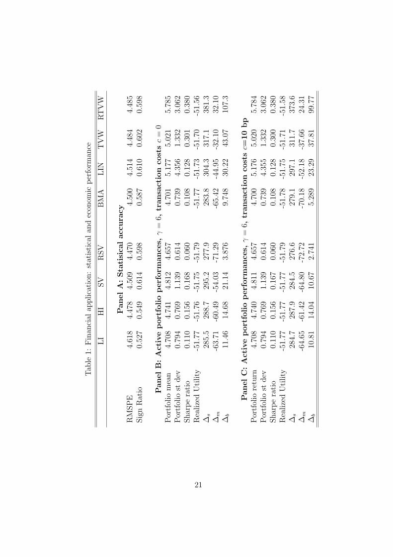
Before we analyze the performance of the different portfolios, we summarize the statisti-

cal accuracy of the excess return forecasts. All the individual models give similar RMSPE

statistics in Table 1, for the RSV model just the smallest and for the LI model the highest.

The sign ratio is the highest for the SV model, but hardly exceeds 60%, indicating low pre-

dictability. Due to this low predictability, small differences in RMSPE may have substantial

economic value. We investigate this in the portfolio exercise. The SV model gives the highest

Sharpe ratio, realized final utility and comparison fees ∆ among the individual models. The

TVW and RTVW combination schemes, however, provide much higher statistics; in partic-

ular RTVW outperforms all the other models in terms of Sharpe ratio and realized utility

value, and all three ∆’s are positive. Figure 1 can help to explain these findings. Individual

models allocate too low weight to the risky asset resulting in low portfolio returns. BMA

has a similar problem. The LIN, TVW and RTVW combinations allocate higher weights to

the stock asset, but RTVW is the only scheme that drastically reduces this weight in bear

market periods as the burst of the internet bubble in 2001-2003 or the recent financial crisis

in the second part of 2007 and 2008. Panel C in Table 1 shows evidence that the findings

are similar when taking into account the presence of medium transaction costs.

The good performance of RTVW as compared to LIN and TVW shows that its robust

flexible structure pays off. The higher portfolio weight of stock in bull markets for RTVW,

as compared to the individual models and BMA, is due to the ‘shrunk’ predictive density.

This ‘shrunk’ excess return distribution is not so much ‘compressed’ that the risky asset’s

portfolio weight switches from 0% to 100% when its mean changes from negative to positive

values. Rather, the parameter and model uncertainty that are incorporated in this ‘shrunk’

predictive density imply an investment strategy with a smooth, ‘moderate’, yet flexible

6We also implement exercises with γ = 4 and γ = 8. Results are qualitatively similar and available uponrequest.

13

evolvement of the risky asset’s portfolio weight over time. Lettau and Van Nieuwerburgh

(2008) find that the uncertainty on the size of steady-state shifts rather than their dates is

responsible for the difficulty of forecasting stock returns in real time. The ‘shrunk’ predictive

density of the RTVW scheme may be particularly informative on the current and future

evolvement of this steady-state, the driving force of return predictability. This may be the

explanation for the RTVW scheme’s good results. We intend to analyze its performance in

other portfolio management exercises in future research, in order to investigate the robustness

of our findings.

4 US real GDP Growth

We now perform an empirical analysis on a key macroeconomic series, the U.S. real Gross

Domestic Product (GDP) growth. We collected real GDP (seasonally adjusted) figures from

the U.S. Department of Commerce, Bureau of Economic Analysis. The left panel of Figure 2

plots the log quarterly GDP level for our sample 1960:Q1 to 2008:Q3 (195 observations) and

shows that GDP has followed an upward sloping pattern but with fluctuations around this

trend. The quarterly growth rate, ln GDPt−ln GDPt−1, shown in the right panel of Figure 2,

underlines these fluctuations with periods of positive changes followed by periods of negative

changes, clearly indicating business cycles; for more details we refer to Harvey, Trimbur, and

Van Dijk (2007). As in the previous section, we apply various linear and nonlinear models

and forecast combinations to assess these models’ suitability in a pseudo-real-time out-of-

sample forecasting exercise. In the forecast exercise we use an initial in-sample period from

1960:Q1 to 1979:Q4 to obtain initial parameter estimates and we forecast the GDP growth

figure for 1980:Q1. We then expand the estimation sample with the value in 1980:Q1, re-

estimating the parameters, and we forecast the next value for 1980:Q2. We continue this

procedure up to the last value and we end up with a total of 115 forecasts.

We apply n = 6 individual time series models to infer and forecast GDP. Four models

are linear specifications, two models are time-varying parameter specifications. The first and

second model are random walk models, without and with drift (RW and RWD). The third

model is the autoregressive (AR) model of order 1. We follow Schotman and Van Dijk (1991)

and specify a weakly informative ‘regularization’ prior that helps to prevent problems that

could be encountered during the estimation using the Gibbs sampler, if a flat prior were

used. The fourth model we apply is an error correction model (ECM). We apply the same

14

model as in De Pooter, Ravazzolo, Segers, and Van Dijk (2008):

∆yt = δ + (ρ1 + ρ2 − 1)(yt−1 − µ− δ(t− 1))− ρ2(∆yt−1 − δ) + εt, εt ∼ N(0, σ2), (27)

which can be rewritten as:

yt− δt = (1−ρ1−ρ2)µ+ρ1(yt−1− δ(t− 1))+ρ2(yt−2− δ(t− 2))+ εt, εt ∼ N(0, σ2). (28)

The prior that we use is an extension of the prior of Schotman and Van Dijk (1991). The

fifth and sixth models are a state-space model (SSM) and its robust extension (RSSM), that

are given by the SV and RSV models of section 3.

We use the root mean square prediction error (RMSPE) to compare different point fore-

casts. Table 2 shows that the random walk models perform poorly. For all other models,

the test of Clark and West (2007) for equal forecasting quality of nested models rejects the

null hypothesis versus the RW model. The AR model is a bit more precise than the ECM.

The models with time varying parameters, SSM and RSSM, perform very well. Figure 3

shows that all models with fixed parameters perform poorly when GDP decreases rapidly

and substantially as in NBER recessions, and it takes some quarters for models to adjust,

in particular in the 2001 recession and the 2008 recession. Time-varying parameter models

seem to cope better with this.

The BMA and RTVW combination schemes provide even better statistics than the SSM

and RSSM models. LIN is the worst averaging scheme; LIN performs similarly to the AR

and ECM models. Figure 4 shows that LIN is performing particularly poorly in the 1980’s

and 1990’s. Weight estimates for this scheme may be highly inaccurate as the number

of individual models is relatively large and instability possibly high. Moreover, Figure 4

indicates that the other averaging schemes react much faster to sharp decreases in GDP.

Especially the RTVW scheme may early indicate recessions: before both the 1991 and 2001

crises its point forecast decreases substantially with approximately 0.5%.

To sum up, our results suggest that model averaging may be very beneficial in business

cycle analysis and forecasting. The combination method must, however, be chosen carefully

and it should cope with estimation efficiency and structural instability, in particular if weights

are estimated in regression equations. Again, more extensive studies should be performed to

investigate the robustness of our findings, for example over different countries and periods.

15

5 Final remarks

The empirical applications have indicated, firstly, that averaging strategies can give higher

predictive quality than selecting the best model; secondly, that properly specified time vary-

ing model weights yield higher forecast accuracy and substantial economic gains compared

with other averaging schemes. The presented results lead to multiple directions for future

research. As we already mentioned, interesting possibilities for further research are a rigor-

ous analysis of the impact of some assumptions – both on theoretical aspects and practical

applications – and an extensive study on the robustness of our findings.

Another topic for further research is to compare our results to other time varying weight

combination schemes, such as regime switching, see e.g. Guidolin and Timmermann (2007),

or schemes that carefully model breaks, see e.g. Ravazzolo, Paap, Van Dijk, and Franses

(2007). For the application to portfolio management, a natural extension is the prediction

of multivariate returns processes. The proposed combination schemes can also be adapted

to the specific prediction of variance, skewness or kurtosis.

Acknowledgements

This paper is a substantial revision and extension of Ravazzolo, Van Dijk, and Verbeek

(2007). We are very grateful to participants of the Conference of the 50-th Anniversary of the

Econometric Institute 2006, and the Conference on Computational Economics and Finance,

Geneva, 2007, for their helpful comments on earlier versions of the paper. Herman K. van

Dijk gratefully acknowledges the financial assistance from the Netherlands Organization of

Research (under grant # 400-07-703). The views expressed in this paper are our own and

do not necessarily reflect the views of Norges Bank (the Central Bank of Norway). Any

remaining errors or shortcomings are the authors’ responsibility.

16

References

Ardia, D., Hoogerheide, L. F., and Van Dijk, H. K. 2009. To Bridge, to Warp or to Wrap? A

comparative study of Monte Carlo methods for efficient evaluation of marginal likelihoods.

Tinbergen institute report 09-017/4.

Barberis, N. 2000. Investing for the Long Run When Returns Are Predictable. Journal of

Finance 55: 225–264.

Bates, J. M., and Granger, C. W. J. 1969. Combination of Forecasts. Operational Research

Quarterly 20: 451–468.

Bouman, S., and Jacobsen, B. 2002. The Halloween Indicator, ‘Sell in May and Go Away’:

Another Puzzle. American Economic Review 92 (5): 1618–1635.

Chib, S. 1995. Marginal Likelihood from the Gibbs Output. Journal of American Statistical

Association 90: 972–985.

Clark, T. E., and West, K. D. 2007. Approximately normal tests for equal predictive accuracy

in nested models. Journal of Econometrics 138 (May): 291–311.

Cremers, K. J. M. 2002. Stock Return Predictability: A Bayesian Model Selection Perspec-

tive. Review of Financial Studies 15: 1223–1249.

De Pooter, M., Ravazzolo, F., Segers, R., and Van Dijk, H. K. 2008. Bayesian Near-Boundary

Analysis in Basci Macroeconomic Time-Series Models. Advances in Econometrics 23: 331–

402.

Draper, D. 1995. Assessment and Propagation of Model Uncertainty. Journal of the Royal

Statistical Society Series B 56: 45–98.

Fernandez, C., Ley, E., and Steel, M. F. J. 2001. Model uncertainty in cross-country growth

regressions. Journal of Applied Econometrics 16: 563–576.

Fleming, J., Kirby, C., and Ostdiek, B. 2001. The Economic Value of Volatility Timing.

Journal of Finance 56: 329–352.

Gerlach, R., Carter, C., and Kohn, R. 2000. Efficient Bayesian Inference for Dynamic Mixture

Models. Journal of the American Statistical Association 95: 819–828.

17

Geweke, J., and Whiteman, C. 2006. Bayesian Forecasting. In G. Elliot, C. Granger, and

A. Timmermann(ed.) Handbook of Economic Forecasting North-Holland.

Giordani, P., and Kohn, R. 2008. Efficient Bayesian Inference for Multiple Change-Point and

Mixture Innovation Models. Journal of Business & Economic Statistics 26: 66–77.

Giordani, P., Kohn, R., and Van Dijk, D. 2007. A Unified Approach to Nonlinearity, Outliers

and Structural Breaks. Journal of Econometrics 137: 112–137.

Giordani, P., and Villani, M. 2008. Forecasting macroeconomic time series with locally adap-

tive signal extraction. Working Paper.

Granger, C. W. J., and Ramanathan, R. 1984. Improved Methods of Combining Forecasts.

Journal of Forecasting 3: 197–204.

Groen, J., Paap, R., and Ravazzolo, F. 2009. Real-Time Inflation Forecasting in a Changing

World. Working paper.

Guidolin, M., and Timmermann, A. 2007. Forecasts of US Short-term Interest Rates: A

Flexible Forecast Combination Approach. forthcoming in Journal of Econometrics.

Hansen, B. E. 2007. Least Squares Model Averaging. Econometrica 75(4): 1175–1189.

Harvey, A. C. 1993. Time Series Models : . Pearson Education.

Harvey, A. C., Trimbur, T. M., and Van Dijk, H. K. 2007. Bayes Estimates of the Cycli-

cal Component in Twentieth Century U.S. GrossDomestic Product. In G. L. Mazzi, and

G. Savio(ed.) Growth and Cycle in the Eurozone Palgrave MacMillan, New York.

Hendry, D. F., and Clements, M. P. 2004. Pooling of Forecasts. Econometric Reviews 122:

47–79.

Hodges, J. 1987. Uncertainty, Policy Analysis and Statistics. Statistical Science 2: 259–291.

Kascha, C., and Ravazzolo, F. 2008. Combining Inflation Density Forecasts. Norges Bank

working paper 2008-22.

Koop, G. 2003. Bayesian Econometrics. West Sussex, England: John Wiley & Sons Ltd.

Leamer, E. 1978. Specification Searches : . New York: Wiley.

18

Lettau, M., and Van Nieuwerburgh, S. 2008. Reconciling the Return Predictability Evidence.

The Review of Financial Studies 21: 1607–1652.

Madigan, D., and Raftery, A. 1994. Model Selection and Accounting for Model Uncertainty in

Graphical Models Using Occam’s Window. Journal of the American Statistical Association

89: 1335–1346.

Marcellino, M. 2004. Forecasting Pooling for Short Time Series of Macroeconomic Variables.

Oxford Bulletin of Economic and Statistics 66: 91–112.

Marquering, W., and Verbeek, M. 2004. The Economic Value of Predicting Stock Index

Returns and Volatility. Journal of Financial and Quantitative Analysis 39 (2): 407–429.

Min, C., and Zellner, A. 1993. Bayesian and Non-Bayesian Methods for Combining Models

and Forecasts with Applications to Forecasting International Growth Rates. Journal of

Econometrics 56: 89–118.

Mitchell, J., and Hall, S. G. 2005. Evaluating, comparing and combining density forecasts

using the KLIC with an application to the Bank of England and NIESER “fan” charts of

inflation.. Oxford Bulletin of Economics and Statistics 67: 995–1033.

Pesaran, M. H., and Timmermann, A. 1995. Predictability of Stock Returns: Robustness

and Economic Significance. Journal of Finance 50: 1201–1228.

Pesaran, M. H., and Timmermann, A. 2002. Market Timing and Return Predictability Under

Model Instability. Journal of Empirical Finance 9: 495–510.

Planas, C., Rossi, A., and Fiorentini, G. 2008. The marginal likelihood of Structural Time

Series Models, with application to the euroarea and US NAIRU. Working Paper Series

21-08, Rimini Centre for Economic Analysis.

Ravazzolo, F., Paap, R., Van Dijk, D., and Franses, P. H. 2007. Bayesian Model Averaging

in the Presence of Structural Breaks. In M. Wohar, and D. Rapach(ed.) Forecasting in the

Presence of Structural Breaks and Model Uncertainty Elsevier.

Ravazzolo, F., Van Dijk, H. K., and Verbeek, M. 2007. Predictive gains from forecast com-

binations using time varying model weights. Econometric institute report 2007-26.

19

Sala-i-Martin, X., Doppelhoffer, G., and Miller, R. 2004. Determinants of long-term growth:

A Bayesian averaging of classical estimates (BACE) approach. American Economic Review

94: 813–835.

Schotman, P., and Van Dijk, H. K. 1991. A Bayesian Analysis of the Unit Root in Real

Exchange Rates. Journal of Econometrics 49: 195–238.

Stock, J. H., and Watson, M. 2004. Combination Forecasts of Output Growth in a Seven-

country Data Set. Journal of Forecasting 23: 405–430.

Strachan, R., and Van Dijk, H. K. 2008. Bayesian Averaging over Many Dynamic Model

Structures with Evidence on the Great Ratios and Liquidity Trap Risk. Tinbergen Institute

report 2008-096/4, Erasmus University Rotterdam.

Terui, N., and Van Dijk, H. K. 2002. Predictability in the Shape of the Term Structure of

Interest Rates. International Journal of Forecasting 18: 421–438.

Timmermann, A. 2006. Forecast Combinations. In G. Elliot, C. W. J. Granger, and A. Tim-

mermann(ed.) Handbook of Economic Forecasting North-Holland.

20

Tab

le1:

Fin

anci

alap

plica

tion

:st

atis

tica

lan

dec

onom

icper

form

ance

LI

HI

SV

RSV

BM

ALIN

TV

WRT

VW

PanelA

:Sta

tisi

calacc

ura

cyR

MSP

E4.

618

4.47

84.

509

4.47

04.

500

4.51

44.

484

4.48

5Sig

nR

atio

0.52

70.

549

0.61

40.

598

0.58

70.

610

0.60

20.

598

PanelB

:A

ctiv

eport

folio

perf

orm

ance

s,γ

=6,

transa

ctio

nco

sts

c=

0Por

tfol

iom

ean

4.70

84.

741

4.81

24.

657

4.70

15.

177

5.02

15.

785

Por

tfol

iost

dev

0.79

40.

769

1.13

90.

614

0.73

94.

356

1.33

23.

062

Shar

pe

rati

o0.

110

0.15

60.

168

0.06

00.

108

0.12

80.

301

0.38

0R

ealize

dU

tility

-51.

77-5

1.76

-51.

75-5

1.79

-51.

77-5

1.73

-51.

70-5

1.56

∆s

285.

528

8.7

295.

227

7.9

283.

830

4.3

317.

138

1.3

∆m

-63.

71-6

0.49

-54.

03-7

1.29

-65.

42-4

4.95

-32.

1032

.10

∆b

11.4

614

.68

21.1

43.

876

9.74

830

.22

43.0

710

7.3

PanelC

:A

ctiv

eport

folio

perf

orm

ance

s,γ

=6,

transa

ctio

nco

sts

c=10

bp

Por

tfol

iore

turn

4.70

84.

740

4.81

14.

657

4.70

05.

176

5.02

05.

784

Por

tfol

iost

dev

0.79

40.

769

1.13

90.

614

0.73

94.

355

1.33

23.

062

Shar

pe

rati

o0.

110

0.15

60.

167

0.06

00.

108

0.12

80.

300

0.38

0R

ealize

dU

tility

-51.

77-5

1.77

-51.

77-5

1.79

-51.

78-5

1.75

-51.

71-5

1.58

∆s

284.

728

7.9

284.

527

6.6

279.

129

7.1

311.

737

3.6

∆m

-64.

65-6

1.42

-64.

80-7

2.72

-70.

18-5

2.18

-37.

6624

.31

∆b

10.8

114

.04

10.6

72.

741

5.28

923

.29

37.8

199

.77

21

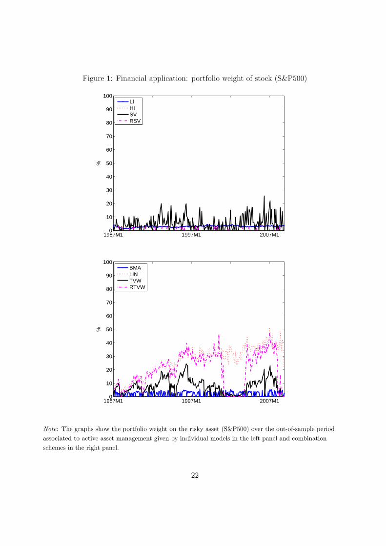
Figure 1: Financial application: portfolio weight of stock (S&P500)

1987M1 1997M1 2007M10

10

20

30

40

50

60

70

80

90

100%

LIHISVRSV

1987M1 1997M1 2007M10

10

20

30

40

50

60

70

80

90

100

%

BMALINTVWRTVW

Note: The graphs show the portfolio weight on the risky asset (S&P500) over the out-of-sample periodassociated to active asset management given by individual models in the left panel and combinationschemes in the right panel.

22

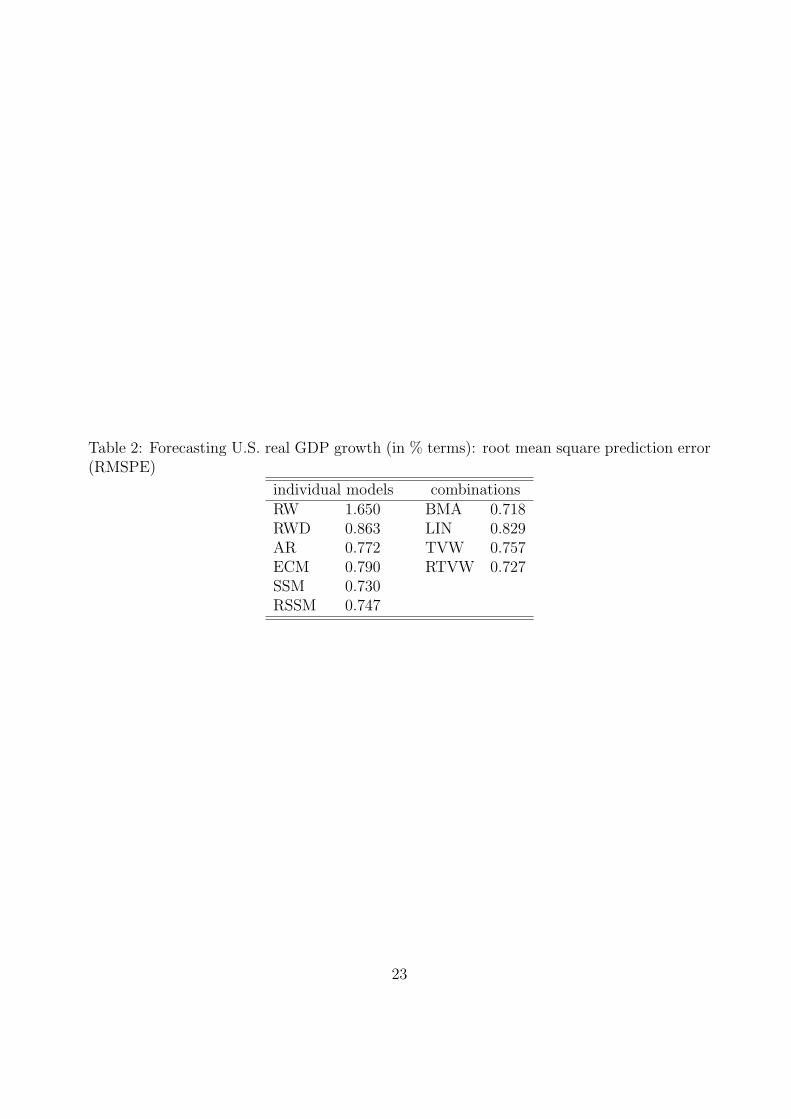
Table 2: Forecasting U.S. real GDP growth (in % terms): root mean square prediction error(RMSPE)

individual models combinationsRW 1.650 BMA 0.718RWD 0.863 LIN 0.829AR 0.772 TVW 0.757ECM 0.790 RTVW 0.727SSM 0.730RSSM 0.747

23

Figure 2: US real GDP

1960Q1 1970Q1 1980Q1 1990Q1 2000Q16

6.5

7

7.5

8

8.5

9

9.5

10

1960Q1 1970Q1 1980Q1 1990Q1 2000Q1−2

−1

0

1

2

3

4

5

6%

Note: Quarterly log levels of U.S. real GDP (left) and quarterly GDP growth rate in % terms (right). Thesample is 1960:Q1 - 2008:Q3.

24

Figure 3: US real GDP: point forecasts

Note: Quarterly U.S. real GDP growth (in %) and point forecasts given by individual models. Verticalbars highlight NBER recession periods.

25

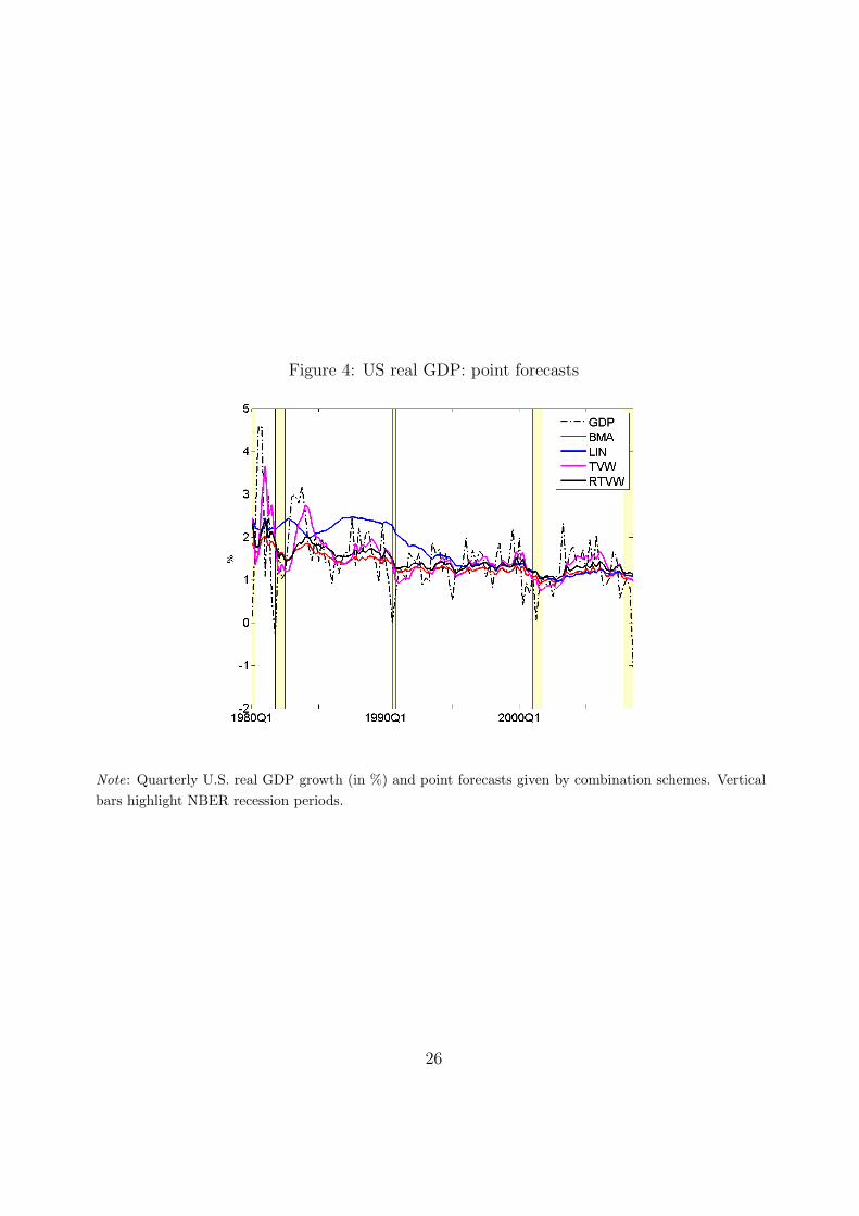
Figure 4: US real GDP: point forecasts

Note: Quarterly U.S. real GDP growth (in %) and point forecasts given by combination schemes. Verticalbars highlight NBER recession periods.

26