EEccoonnoomm iiccss PPrrooggrraamm WWoorrkkiinngg PPaapp eerr SSeerr iieess

Forecasting Chinese Households’

Demand from Home

Production

Yabin Wang*

University of California, Santa Cruz

June 2013

EEPPWWPP ##1133 –– 0011

Economics Program

845 Third Avenue

New York, NY 10022-6679

Tel. 212-759-0900

www.conference-board .org/ economics

Forecasting Chinese Households’ Demand from Home

Production∗

Yabin Wang†

University of California, Santa Cruz

June 12, 2013

Abstract

As the Chinese market economy expands and market institutions become stronger, therewill be more incentives for Chinese households to substitute market activity for home pro-duction. The goal of this paper is to provide a quantitative analysis of the potential Chineseconsumer demand for household services. Using dataset from the American Time Use Surveyand the China Health and Nutrition Survey, I compare households’ demand for services andhome production between US and China. A standard choice-theoretic model of the householdis used to estimate the structural parameters and to quantitatively forecast Chinese households’service demand.

1 Introduction

Over the next decades emerging markets have the potential to become a major source of consumer

demand in the world economy. The Chinese economy will play an important role, not only for

its size, but also because it is bound to experience a dramatic change in its growth model . Three

factors that will reshape China’s development are: 1) an impending shortage of cheap labor, a

so-called Lewis turning point, 2) the current account imbalance and 3) a demographic transition

that will bring about a large increase in the dependency ratio. Among the other changes necessary

for China to avoid a middle-income trap, its growth model will have to shift towards domestic

consumption. Where the demand of Chinese households is heading becomes a question of ut-

most importance. This paper explores the potential consumer demand arising through a specific

mechanism— changes in home production. As China’s market economy develops, more and more

needs that have been addressed within the household through home production will have to be

satisfied by the market.∗This paper was written during my Robert H. McGuckin Fellowship in 2012 at The Conference Board. I thank

Ataman Ozyildirim, Vivian Chen, Bart van Ark, and Louise Keely for their comments and helpful suggestions. Allremaining errors are mine.

†Economics Department, 494 E2 Building, Santa Cruz, CA 95064. E-mail: ynwang@ucsc.edu.

1

This argument is based on the hypothesis that home production in China has absorbed a dis-

proportionately high fraction of economic activity because of distortions typical of a developing

country, such as market failures and low opportunity cost of time for individuals in their 50s and

60s. I provide support for this hypothesis by a comparative study of time allocation between China

and US. I use data from the American Time Use Survey and the Chinese Health and Nutrition Sur-

vey between 2004 and 2009. The results offer a very clear picture. While home production hours

are higher in China than in the US, in the past decade time allocation in China has tended towards

US levels. However, the time allocation pattern shown by Chinese data still display features that

are typical of a developing country. First, retired individuals are very active in home production

(in China a retired individual works at home 5 hours per week more than an American retired

individual), which is due to the low statutory retirement age and informal intergenerational trans-

fers. Second, there is a large and growing gender gap in home production hours (the gender gap

is around 5 hours per week in US and around 10 hours per week in China).

If time allocation in China converges to US configurations or some of its most striking imbal-

ances are eliminated (e.g. reducing the gender gap to US levels), then important adjustments in

average home work hours and home production are going to take place. The goal of this paper is to

measure the effects of these adjustments on consumer demand. Everything else equal, a reduction

in home production results in an equivalent increase in demand for market substitutes (such as

dining, housecleaning, home repairs and care work). Thus by valuing the changes in time spent in

home production it is possible to obtain an estimate of the potential demand for market susbtitues.

As regards the methodolgy of this paper, I evaluate home output first using two standard

methods: the market cost method and the opportunity cost method. Then I introduce an additional

method that uses a structural approach. I estimate the structural parameters of a standard choice-

theoretic model of the household . Results show that the estimated home output value using

the structural method is close to the other two methods when applied to the Chinese dataset.

The structural method has a number of advantages compared to the other two methods, most

importantly it allows to take into account the role of retired people, technology and capital, such

as electrical appliances.

The final goal of this paper is to quantitatively forecast Chinese households’ service demand in

response to the changing economic situation. I study a number of different scenarios. If China fully

converges to the US level of home production time, the weekly increase in consumer demand as a

proportion of a typical household weekly income is forecasted to be in the range 8-12%. Allowing

2

for an increase in the usage of electrical appliances (and thus limiting the need to resort to market

goods) provides a lower bound to the forecast, around 4%. Policies that address the gender gap or

the retirement gap can also generate relevant increases in consumer demand.

The paper is organized as follows. Part 2 provides a review of related literature. In part 3

I describe the patterns of time allocation in China and in the US. Part 4 offers two traditional

methods and a theoretical model of home production that can be used to analyze the data. In

part 5, I quantify the potential changes in consumer expenditure. Part 6 offers some concluding

remarks.

2 Review of the Literature

This paper contributes to several strands of the literature:

1. The measurement of home production in a national accounting framework.

The problem of measuring the value of home production dates back to Nordhaus and Tobin

(1972), but there have been many contributions since then. Key methodologies and findings

are surveyed in Hawrylyshyn (2012). Empirical studies that attempt to measure the value

of household production typically indicate that it is large. For example, the survey study

of Hawrylyshyn (2012) finds that estimates of home produced output are around one third

of measured gross national product. To my knowledge this literature does not include any

empirical comparative study between developing and developed countries.

2. Theory of household time allocation

The theory of home production can be dated back to Gary Becker (1965)’s seminal paper

that modeled consumer behavior using a household production function approach. This

approach sees agents as choosing not simply between work and leisure, but between work

in the home, work in the market and leisure. These theories have been used to study many

different issues, such as long run trends in time use, lifecycle patterns of expenditures and

labor supply and the allocation of time over the business cycle, as surveyed by Aguiar et al.

(2012).

The relation between home production and economic development has not been a major

topic in this literature yet. A key paper is Parente et al. (2000). The authors introduce home

production into the neoclassical growth model. They assume that differences in economic de-

3

velopment arise from policies that distort capital accumulation. They find that such policies

decrease hours worked in the market, increasing home production hours, and this magni-

fies the effect on income. The predictions of this model have not been tested systematically,

although a cross-country study would be feasible given the current availability of time use

data. My comparative study of China and US is perhaps the first piece of evidence in support

of this theory.

Additionally studies of long-run trends in time use may also be relevant to the development

issue. For instance, Ramey (2009) shows that in the US from 1900 to 2005 older invididuals

took over more home production through time from the working-age female, resulting in

an increasing female labor force participation. In a study on Russian data, Gronau (2006)

finds that the switch from a controlled economy to a market economy resulted in significant

increase in home productivity and an increase in the free time enjoyed by both Russian men

and women.

3. Chinese economy

There is a large and growing literature on the economics of Chinese households, but it fo-

cuses mainly on issues such as savings and migration. There is no previous study of time

allocation in Chinese families. My research contributes also to the macroeconomic literature

on the Chinese economy. Many studies have argued that China’s private consumption is

exceptionally low (for example Kuo and N’Diaye 2010). The home production framework

I use distinguishes between households’ consumption and demand. While China’s private

demand is low, aggregate household consumption is larger, because it is satisfied in part by

home production. Thus, rebalancing the Chinese economy towards more private demand is

also a matter of shifting consumption from the household into the market. A further benefit

of this approach is to help quantifying the potential gains in private demand.

3 Time Use in China and in the US

A. Data Description

The datasets that I use in this paper are the China Health and Nutrition Survey (CHNS) and the

American Time Use Survey (ATUS).

The CHNS survey data is documented from 1989 to 2009 that covers nine provinces. The survey

has information on time allocation among home work, market work and leisure. Time records

4

include the time spent on cooking, cleaning, housework and childcare. Other key socio-economic

variables such as demographic information and income are also recorded. Table 1 gives a summary

of the CHNS sample. Table 2 focuses on home production time at household level1. The dataset

covers around 15300 observations at individual level, and 4337 observations at household level2.

In my study, I define home production as hours per week spent on taking care of children, and

certain kinds of housework including doing grocery, cooking, cleaning, and doing laundry. Work

hours is defined as weekly working hours spent on primary occupation. Leisure hours include

weekly time spent on physical activities (such as martial arts, gymnastics, swimming, track & field

and etc.) and sedentary activity (such as watching tv and video, reading, surfing on the internet

and so on.) Annual income is calculated as annual salary in the previous year plus the total value

of all bonuses for the previous entire year. Older female is defined as a female who is no younger

than 55 years old and older male is defined as a male who is no younger than 60 years old3.

1Table1 uses waves from 1997 to 2009 to ensure a better quality of the dataset.To obtain a more complete dataset forkey variables, Table2 uses panel for the year 2004 to 2009, which contains three waves of survey: 2004, 2006 and 2009.

2The educational attainment is documented as education index, and the average education of 20.13 roughly repre-sents the sample mean is about 1 year lower middle school of formal education.

3The way I define older female and older male is consistent with the retirement age in China.

5

Table 1: Descriptive Statistics - CHNS

Obs Mean Std.Err. Min Max

A. Demographic Variables

Age 15659 47.04 14.3314 13.2 93.13

Fraction female 15659 .53 .4993 0 1

Married 15659 .87 .3358 0 1

Education 15500 20.13 8.4494 0 36

Fraction retired 15659 .18 .3836 0 1

Household size 15659 1.94 .8841 1 7

Number of olders 15659 .46 .7105 0 3

B. Geographic Variables

Rural 15659 .55 .4972 0 1

Urban 15659 .45 .4971 0 1

C. Time Allocation

Work hours 12505 39.71 19.9694 1 126

Home hours 15659 15.73 17.8016 0 266

Leisure hours 14827 19.49 15.9163 0 248

D. Income

Annual income 5110 15580.72 20973.92 480 480000

Retirement wage 2720 13726.28 11131.31 240 119988

Table 2: Statistics on Home Production Time - CHNS

Obs Mean Std.Err. Min Max

A. Different Age Groups

All age cohorts 14287 15.72 16.9187 0 266.00

Young female 4961 21.88 19.0661 0 266.00

Young male 4827 7.29 10.3710 0 151.50

Older female 2975 23.03 17.0262 0 227.33

Older male 2064 10.08 12.1302 0 165.50

B. Household Level

Individual 7648 14.11 16.6121 0 227.33

Spouse 6876 18.16 17.1378 .12 227.33

Elder mother 853 25.05 19.6719 1.17 162.75

Elder father 598 11.52 12.0115 .12 94.00

Household 4145 32.21 23.4179 0.47 248.50

6

Table 3: Provincial Level Summary - CHNS

Province Obs Age Female Edu Retired Married Urban Income Work Home Leisure

Liaoning 1819 53.13 .55 22.48 .30 .90 .59 15830 44.99 16.87 21.62

Heilongjiang 1579 47.91 .52 22.68 .15 .91 .45 16964 43.51 16.22 20.57

Jiangsu 2517 52.48 .55 19.30 .22 .89 .54 16196 38.83 16.49 17.69

Shandong 1472 51.17 .51 19.74 .25 .86 .54 15200 45.26 14.04 22.26

Henan 1640 48.90 .53 19.52 .12 .87 .34 13279 38.52 17.32 18.73

Hubei 1657 50.38 .53 19.65 .17 .87 .40 15200 37.42 15.84 19.60

Hunan 1269 50.49 .49 22.00 .17 .86 .50 20677 39.53 15.70 23.28

Guangxi 1806 49.29 .51 20.16 .13 .82 .35 11162 38.90 16.26 17.23

Guizhou 1900 51.15 .53 16.85 .09 .85 .28 15473 34.03 16.28 16.79

National 15696 50.68 .53 20.13 .18 .87 .45 15581 39.71 12.30 19.49

The ATUS survey is a multi-year survey from 2003 to 2010. It contains about 112000 observa-

tions. The survey provides information on the amount of time people spend in many activities,

such as housework, childcare, exercising, and relaxing. Demographic information such as sex,

age, educational attainment, and income are also available. Table 4 gives a summary of the ATUS

sample. Table 5 focuses on home production time.

7

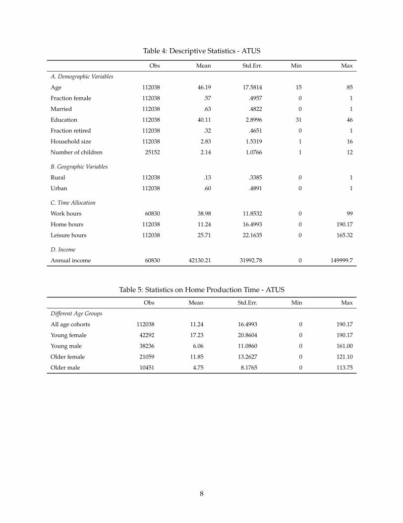
Table 4: Descriptive Statistics - ATUS

Obs Mean Std.Err. Min Max

A. Demographic Variables

Age 112038 46.19 17.5814 15 85

Fraction female 112038 .57 .4957 0 1

Married 112038 .63 .4822 0 1

Education 112038 40.11 2.8996 31 46

Fraction retired 112038 .32 .4651 0 1

Household size 112038 2.83 1.5319 1 16

Number of children 25152 2.14 1.0766 1 12

B. Geographic Variables

Rural 112038 .13 .3385 0 1

Urban 112038 .60 .4891 0 1

C. Time Allocation

Work hours 60830 38.98 11.8532 0 99

Home hours 112038 11.24 16.4993 0 190.17

Leisure hours 112038 25.71 22.1635 0 165.32

D. Income

Annual income 60830 42130.21 31992.78 0 149999.7

Table 5: Statistics on Home Production Time - ATUS

Obs Mean Std.Err. Min Max

Different Age Groups

All age cohorts 112038 11.24 16.4993 0 190.17

Young female 42292 17.23 20.8604 0 190.17

Young male 38236 6.06 11.0860 0 161.00

Older female 21059 11.85 13.2627 0 121.10

Older male 10451 4.75 8.1765 0 113.75

8

B. A Converging Pattern in Time Allocation between China and US

Figure 1: Hours at Work, Home and Leisure over Time

1020

3040

Hou

rs p

er w

eek

2004 2005 2006 2007 2008 2009survey year

Home China Home USWork China Work US Leisure China Leisure US

Source: Survey data from CHNS and ATUS

Time Allocation over Time

Figure1 shows the general trend of average hours per week people spend in working on the job,

doing home work and enjoying leisure for the survey years 2004, 2006 and 2009 for both Chinese

and US datasets. I report time use at the individual level. The average hours per week spent in

doing home work for Chinese individuals (solid orange line) drop significantly from 18 hours in

2004 to 13 hours in 2009, approaching the overall level of American individual’s average home

working hours (solid blue line). Over this time period, the average working hours per week in

China only slightly increase from 38 to 40 hours (dashed orange line), indicating that only a small

proportion of time reduction from home work goes to market work in China. There is a steady

increase in the amount of hours spent in leisure during the same time range (dotted orange line).

In general, Chinese people spend more time at home work compared to American people, but

less time at leisure. However, this difference is becoming less striking over the years due to the

economic growth in China. One explanation is that increases in the real wage in China have both

income and substitution effects, providing incentives for many individuals to substitute leisure

and market activity for home production. Secondly, the market for services suffers from a number

of imperfections in developing countries and, as it is well known, is especially underdeveloped

in China. However, this situation is rapidly changing. As the Chinese market economy expands

and market institutions become stronger, the imperfections in the service sector are disappearing.

9

These two factors may lead to a further reduction in the home production time allocated by Chi-

nese households, resulting in a converging pattern of home production between US and China.

C. The Key Role of Retired Individuals in China

Figure 2: Home Production for Retired vs. Non-Retired Individuals10

1520

25H

ours

per

wee

k sp

end

on h

ouse

wor

k

2004 2005 2006 2007 2008 2009survey year

Retired China Non-retired ChinaRetired US Non-retired US

Home Production for Retired and Non-Retired

It is useful to look how home production varies with retirement status. Figure 2 shows how home

production hours have changed for retired vs. non-retired individuals from 2004 to 2009. For

both countries, a retired individual on average spends more time on housework than a non-retired

individual. The gap of home production between retired and non-retired appears to be larger in

China than in US.

One reason why the retired gap is large in China is that the retirement age in China is relatively

low compared to more developed countries: the Chinese statutory retirement age for blue-collar

women is 55 and for blue-collar men is 60. The combination of a low statutory retirement age

and increased longevity has resulted in a low opportunity cost of time for individuals in their

50s and 60s. A complementary explanation of the different participation level of old people in

home production is that there is a stronger pattern of intergenerational transfers in China. Tradi-

tional family-based informal mechanisms of support for the elderly give rise to an upward transfer

within households in China, from younger couple to old parents (see for example Cai et al. 2006).

While elders rely on adult children for support, they also in turn provide their children with ser-

vices (Lee and Xiao 1998).

10

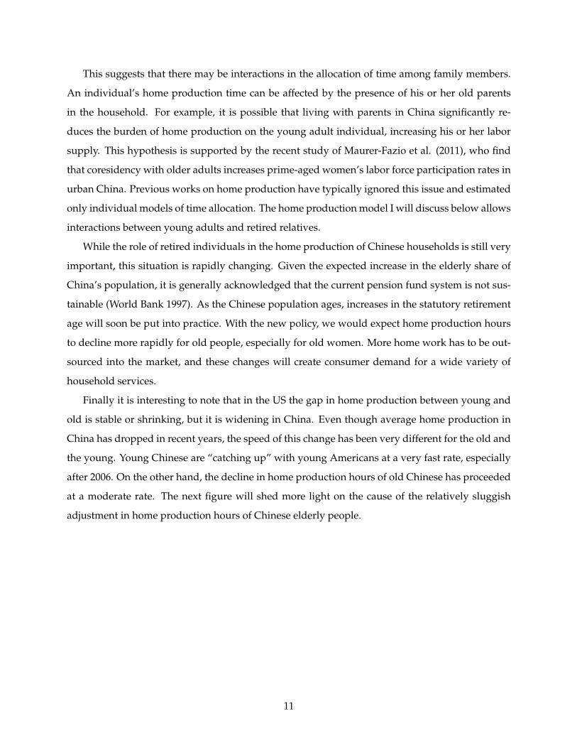
This suggests that there may be interactions in the allocation of time among family members.

An individual’s home production time can be affected by the presence of his or her old parents

in the household. For example, it is possible that living with parents in China significantly re-

duces the burden of home production on the young adult individual, increasing his or her labor

supply. This hypothesis is supported by the recent study of Maurer-Fazio et al. (2011), who find

that coresidency with older adults increases prime-aged women’s labor force participation rates in

urban China. Previous works on home production have typically ignored this issue and estimated

only individual models of time allocation. The home production model I will discuss below allows

interactions between young adults and retired relatives.

While the role of retired individuals in the home production of Chinese households is still very

important, this situation is rapidly changing. Given the expected increase in the elderly share of

China’s population, it is generally acknowledged that the current pension fund system is not sus-

tainable (World Bank 1997). As the Chinese population ages, increases in the statutory retirement

age will soon be put into practice. With the new policy, we would expect home production hours

to decline more rapidly for old people, especially for old women. More home work has to be out-

sourced into the market, and these changes will create consumer demand for a wide variety of

household services.

Finally it is interesting to note that in the US the gap in home production between young and

old is stable or shrinking, but it is widening in China. Even though average home production in

China has dropped in recent years, the speed of this change has been very different for the old and

the young. Young Chinese are “catching up” with young Americans at a very fast rate, especially

after 2006. On the other hand, the decline in home production hours of old Chinese has proceeded

at a moderate rate. The next figure will shed more light on the cause of the relatively sluggish

adjustment in home production hours of Chinese elderly people.

11

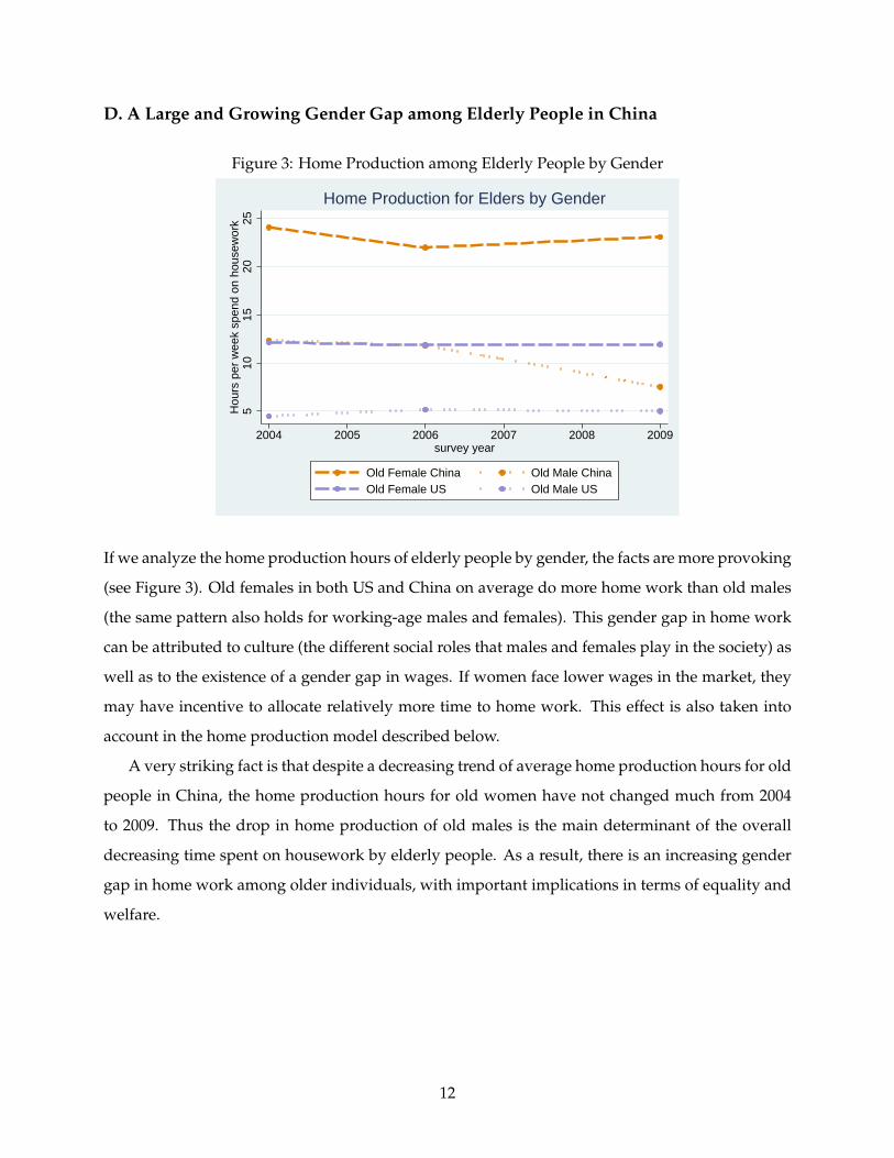
D. A Large and Growing Gender Gap among Elderly People in China

Figure 3: Home Production among Elderly People by Gender

510

1520

25H

ours

per

wee

k sp

end

on h

ouse

wor

k

2004 2005 2006 2007 2008 2009survey year

Old Female China Old Male ChinaOld Female US Old Male US

Home Production for Elders by Gender

If we analyze the home production hours of elderly people by gender, the facts are more provoking

(see Figure 3). Old females in both US and China on average do more home work than old males

(the same pattern also holds for working-age males and females). This gender gap in home work

can be attributed to culture (the different social roles that males and females play in the society) as

well as to the existence of a gender gap in wages. If women face lower wages in the market, they

may have incentive to allocate relatively more time to home work. This effect is also taken into

account in the home production model described below.

A very striking fact is that despite a decreasing trend of average home production hours for old

people in China, the home production hours for old women have not changed much from 2004

to 2009. Thus the drop in home production of old males is the main determinant of the overall

decreasing time spent on housework by elderly people. As a result, there is an increasing gender

gap in home work among older individuals, with important implications in terms of equality and

welfare.

12

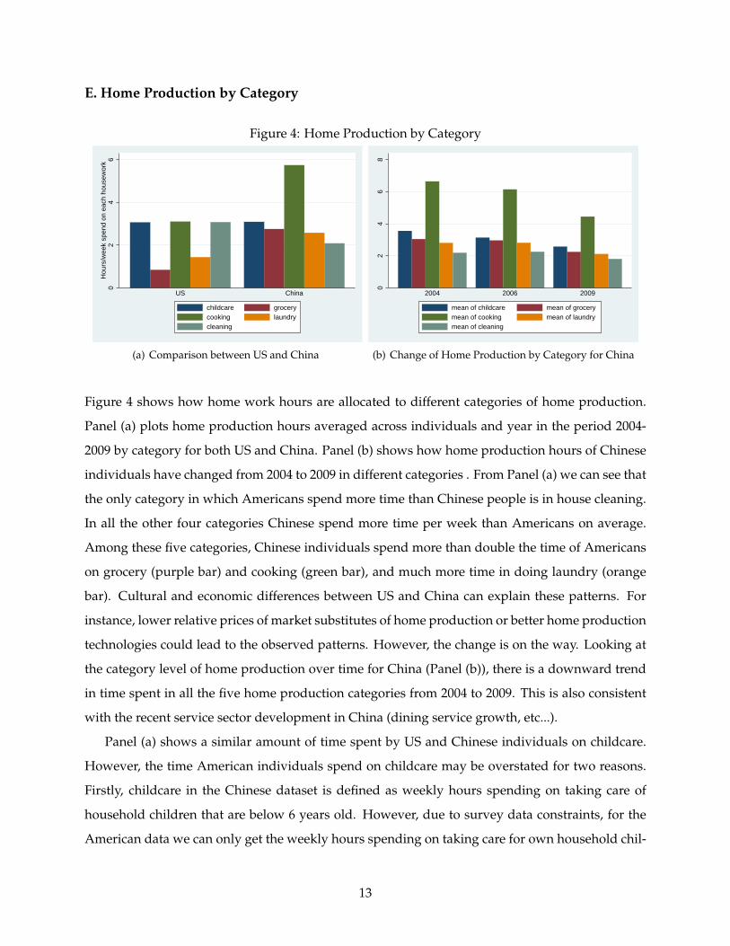
E. Home Production by Category

Figure 4: Home Production by Category

02

46

Hou

rs/w

eek

spen

d on

eac

h ho

usew

ork

US China

childcare grocerycooking laundrycleaning

(a) Comparison between US and China

02

46

8

2004 2006 2009

mean of childcare mean of grocerymean of cooking mean of laundrymean of cleaning

(b) Change of Home Production by Category for China

Figure 4 shows how home work hours are allocated to different categories of home production.

Panel (a) plots home production hours averaged across individuals and year in the period 2004-

2009 by category for both US and China. Panel (b) shows how home production hours of Chinese

individuals have changed from 2004 to 2009 in different categories . From Panel (a) we can see that

the only category in which Americans spend more time than Chinese people is in house cleaning.

In all the other four categories Chinese spend more time per week than Americans on average.

Among these five categories, Chinese individuals spend more than double the time of Americans

on grocery (purple bar) and cooking (green bar), and much more time in doing laundry (orange

bar). Cultural and economic differences between US and China can explain these patterns. For

instance, lower relative prices of market substitutes of home production or better home production

technologies could lead to the observed patterns. However, the change is on the way. Looking at

the category level of home production over time for China (Panel (b)), there is a downward trend

in time spent in all the five home production categories from 2004 to 2009. This is also consistent

with the recent service sector development in China (dining service growth, etc...).

Panel (a) shows a similar amount of time spent by US and Chinese individuals on childcare.

However, the time American individuals spend on childcare may be overstated for two reasons.

Firstly, childcare in the Chinese dataset is defined as weekly hours spending on taking care of

household children that are below 6 years old. However, due to survey data constraints, for the

American data we can only get the weekly hours spending on taking care for own household chil-

13

dren under 13 years old (while the youngest child is below 6 years old). Secondly, based on the

survey data, the average number of children for a US household is around 2 while for Chinese

households is only 1. Similarly, the average American household size is 3 while the average Chi-

nese household size is around 2. This may also explain why Americans spend more time in house

cleaning at the individual level.

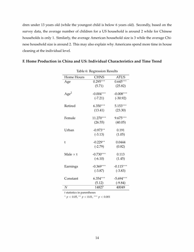
F. Home Production in China and US: Individual Characteristics and Time Trend

Table 6: Regression Results

Home Hours CHNS ATUSAge 0.295∗∗∗ 0.645∗∗∗

(5.71) (25.82)

Age2 -0.004∗∗∗ -0.008∗∗∗

(-7.21) (-30.92)

Retired 6.350∗∗∗ 5.153∗∗∗

(13.41) (23.30)

Female 11.270∗∗∗ 9.675∗∗∗

(26.55) (40.05)

Urban -0.973∗∗ 0.191(-3.13) (1.05)

t -0.229∗∗ 0.0444(-2.79) (0.82)

Male× t -0.730∗∗∗ 0.113(-6.10) (1.45)

Earnings -0.369∗∗∗ -0.115∗∗∗

(-3.87) (-3.83)

Constant 6.354∗∗∗ -5.694∗∗∗

(5.12) (-9.84)N 14827 40049t statistics in parentheses∗ p < 0.05, ∗∗ p < 0.01, ∗∗∗ p < 0.001

14

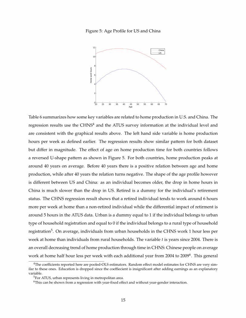
Figure 5: Age Profile for US and China

20 25 30 35 40 45 50 55 60 65 700

2

4

6

8

10

12

Age

Hom

e w

ork

hour

s

ChinaUS

Table 6 summarizes how some key variables are related to home production in U.S. and China. The

regression results use the CHNS4 and the ATUS survey information at the individual level and

are consistent with the graphical results above. The left hand side variable is home production

hours per week as defined earlier. The regression results show similar pattern for both dataset

but differ in magnitude. The effect of age on home production time for both countries follows

a reversed U-shape pattern as shown in Figure 5. For both countries, home production peaks at

around 40 years on average. Before 40 years there is a positive relation between age and home

production, while after 40 years the relation turns negative. The shape of the age profile however

is different between US and China: as an individual becomes older, the drop in home hours in

China is much slower than the drop in US. Retired is a dummy for the individual’s retirement

status. The CHNS regression result shows that a retired individual tends to work around 6 hours

more per week at home than a non-retired individual while the differential impact of retirment is

around 5 hours in the ATUS data. Urban is a dummy equal to 1 if the individual belongs to urban

type of household registration and equal to 0 if the individual belongs to a rural type of household

registration5. On average, individuals from urban households in the CHNS work 1 hour less per

week at home than individuals from rural households. The variable t is years since 2004. There is

an overall decreasing trend of home production through time in CHNS: Chinese people on average

work at home half hour less per week with each additional year from 2004 to 20096. This general

4The coefficients reported here are pooled-OLS estimators. Random effect model estimates for CHNS are very sim-ilar to these ones. Education is dropped since the coeffiecient is insignificant after adding earnings as an explanatoryvariable.

5For ATUS, urban represents living in metropolitan area.6This can be shown from a regression with year-fixed effect and without year-gender interaction.

15

trend is likely to reflect some changes in the macroeconomy, such as a decline in market prices

of household services. In the table I allow for a different trend for females and males. Female is

a dummy variable equal to one if the individual is a woman. Male× t is an interaction term for

addressing both gender and time effects. The estimation results demonstrate a significant effect

of gender on the hours of housework. From 2004 to 2009, home production hours per week for

male individuals decrease around 1 hour every year, while the weekly home production hours

for female individuals only decrease 13 mins every year. Thus, the gap in home production time

between women and men increases over time: women spend 11 home production hours per week

more than men in 2004. However, in 2006 this number reaches roughly 12.3 hours per week, and

further rises to around 14.75 hours per week in 20097. Finally, earnings are negatively related to

home production in both dataset: if weekly income increases by around 30 dollars, weekly home

production hours in CHNS fall by around 20 mins while in ATUS only fall by 1 min.

4 The Value of Home Production

In the past four decades, there have been many attempts to measure home production within a

national accounting framework (for a survey see Hawrylyshyn (2012)). This literature has devel-

oped and applied a standard methodology. In order to simplify the discussion I introduce some

notation that I will expand later. Consider an individual with market wage W. Let H and fH re-

spectively be the hours of home production and the home marginal product of the individual. Let

XH be home production output and XM some close substitute for home production available in the

market. Let p be the market price of the good and WX the market wage paid to labor for producing

XM. The monetary value of the individual’s home production, V, is ideally given by V = pXH.

However, XH is not observable (or very difficult to measure) and p may be difficult to compute as

well. Thus the literature has usually proceeded by valuing the inputs to home production, namely

H. There are essentially two standard methods of evaluating the productive services rendered by

family members at home: (a) evaluating time inputs at the market cost, and (b) evaluating time

inputs at their opportunity costs. In the next two subsections I will describe the two methods and

how to apply them to the CHNS data. Then I will discuss some of the limitations of these methods

and introduce a structural method based on estimation of the home production function.

7The estimates of the coefficients on urban, t, and Male× t from the ATUS dataset are not significant, implying thatthere is no significant change in home production over time since 2004, nor a significant change in the gender gap overtime.

16

4.1 The Market Cost Method

With the market cost method, the individual’s hours of home work are evaluated at the observed

(nominal) wage in the markets for services that are substitutes to home work:

VMC = H ·WX (1)

I calculate WX as the average nominal wage of workers working in the household service sectors.

First I extract a subsample of 871 observations who work in the household service sector based on

their primary occupation from the individual questionnaire8, then I compute the mean wages of

household service workers across years and provinces, and finally assign them to home hours to

obtain the home output value. I illustrate the result of this valuation method in section 5 (see table

9).

4.2 The Opportunity Cost Method

With the opportunity cost method, the individual’s hours of home work are evaluated at her

marginal opportunity cost, given by her own net wage:

VOC = H ·W (2)

The underlying argument, founded for example in Becker (1965)’s seminal paper, is that the opti-

mal choice of home work hours requires the nominal marginal product at home (p · fH) to be equal

to the market wage: p · fH = W. Thus V ' p · fH · H = W · H.

As discussed in the literature, this method cannot be directly applied to individuals who work

at home but not in the market (such as retired people). There are several different ways to impute

a notional wage to individuals that are not employed, as discussed in Sharpe and Abdelghany

(1997). Here I will use one of the most popular methods, based on Heckman’s (1979) procedure to

correct for selectivity bias.

This procedure involves two steps. I regress the probability of an individual working in the

market, measured by Work ≡ 1− Retired, on a number of control variables and two identifying

variables, namely age and age squared. These two variables are assumed to affect the probability of

participation in the labor market, but are assumed not to influence wages. I estimate the following

8These observatioins are identified as service workers, which include housekeeper, cook, waiter, doorkeeper, hair-dresser, counter salesperson, launderer and child care worker)

17

Probit model:

Pr[Work = 1] = a0 + a1edu + a2urban + a3 f emale + a4married + a5t + a6age + a7age2 (3)

where education is an index, urban is a dummy variable that equals one if the individual holds an

urban registration and zero otherwise and t controls for the year. In the second step, I estimate the

following wage equation:

log(W) = b0 + b1edu + b2urban + b3 f emale + b4married + b5t + b6λ̂ (4)

where λ̂ is the estimated inverse of the Mills ratio generated by the Probit equation. The results of

this two-step estimation are presented in Table 7.

Finally, it is possible to use the estimates of equation 4 to impute a notional wage for retired

individuals, given their personal characteristics. Given this notional wage, W, and the individual

home production hours, H, the individual’s value of home production can be computed using the

opportunity cost method as VOC = H ·W. I apply the opportunity cost method to both working

and retired individuals and illustrate the results in section 5 (see Table 9).

18

Table 7: Two-Stage Heckman’s Estimation of Wage Equation

(1)log(w)

log(w)Edu 0.044∗∗∗

(18.59)

Urban 0.317∗∗∗

(9.73)

Female -0.272∗∗∗

(-12.72)

Married 0.156∗∗∗

(5.18)

t 0.121∗∗∗

(23.92)

Constant -0.046(-0.45)

selectAge 0.086∗∗∗

(12.46)

Age2 -0.001∗∗∗

(-18.67)

Edu 0.037∗∗∗

(16.91)

Urban 1.005∗∗∗

(34.25)

Female -0.316∗∗∗

(-12.11)

Married -0.050(-1.13)

t 0.054∗∗∗

(8.92)

Constant -2.517∗∗∗

(-16.68)Millsλ 0.205∗∗∗

(5.36)N 14822t statistics in parentheses∗ p < 0.05, ∗∗ p < 0.01, ∗∗∗ p < 0.001

4.3 Structural method

While the market cost and opportunity cost methods are standard in the valuation literature, here

I present a third methodology based on the theory of home production that is more consistent with

basic economic principles. The two standard methods of valuing home work suffer from a number

19

of limitations. First, both methods will underestimate the true value of home production if there

are diminishing returns to home work. This fact has been overlooked in the accounting literature,

but was pointed out in a passage of Gronau 1977 (p. 1122):

“the product of the average wage rate and the number of hours worked at home there-

fore understates the value of home production to the extent that diminishing marginal

productivity prevails. This imputation does not account for the rent (i.e., the producer’s

surplus) accruing to a person who is self-employed in his own home”.

Similarly, standard valuation methods fail to capture the value of potential complementarities

among the household members’ home production hours (joint rents). More importantly, these

methods do not allow a direct treatment of technology and capital (e.g. electrical appliances). The

structural approach I present below, based on a modeling of the home production function, deals

with all these issues. Finally, the structural approach provides a way to evaluate the contribution

of non-employed individuals more precisely than the imputation methods used in opportunity

cost valuation.

I describe a simple home production model, similar in many respects to standard models in

the literature, such as Gronau (1977, 1980) and Graham and Green (1984). Gronau (1977, 1980)

constructs a model for a married woman where the husband’s decision is exogenous. It is a model

of one individual who allocates time among market work, home production and leisure. The

model assumes that home time produces a good that is a perfect substitute for a composite good

that may be purchased on the market. Gronau tests his model’s predictions by using data from

the 1972 panel of the Michigan Study of Income Dynamics. Graham and Green (1984) extend the

Gronau model to a two wage-earner household and allow home production and leisure to overlap

to some degree. Their focus is on the estimation of the household consumption technology that

consists of a Cobb-Douglas function and a “jointness” function. They estimate an equation for the

home production time for married women using data from the Panel Study of Income Dynamics

for 1976 and provide estimates for the value of home production.

The main difference of my model from previous works is that I allow some members of the

household not to participate in the labor market. This extension makes it possible to take into

account the role of retired inviduals, which is very important as the data suggest. I try to keep

other aspects of the model as simple as possible.

As an illustration, I consider a household with three members: wife, husband and an old rel-

ative that is retired. The model can be easily extended to include more complicated household

20

structures and in the estimation I will allow an arbitrary number of working and non-working

household members. I assume there is no joint use of time for work at home and leisure and that

working at home and working in the market are perfect substitutes. I use a unitary model of the

household, where the members maximize household utility. Household utility is given by:

U(C, Lh, Lw, Lo) (5)

where C, Lh, Lw and Lo are household’s consumption, leisure of the husband, the wife and the

elder relative respectively.

Total consumption of household services (C) can be obtained from the market or produced at

home:

C = XM + XH (6)

where XM represents goods purchased in the market and XH represents goods produced at home

(measured in the same units as market-purchased goods). Clearly, here I focus on market and

household products that are perfect substitutes in consumption.

Home production is described by the following technology:

XH = f (Hh, Hw, Ho) (7)

where Hh, Hw and Ho represent the time spent in home production by the three members. This pro-

duction function is twice continuously differentiable with positive first derivatives and is strictly

concave. For simplicity, I drop the use of market-purchased intermediate inputs in this formula-

tion9.

The household faces a budget constraint:

pXM = WhNh + WwNw + v (8)

where v is nonlabor income (including the retirement income of the elder relative) net of expen-

diture on other goods. Wh and Ww are hourly wages, and Nh and Nw are hours of work of the

husband and wife respectively.

9Graham and Green include a market-purchased intermediate inputs, and they consider the possibility that thehuman capital of the household members may be more suited to market work than to home production.

21

In addition, each household member faces a time allocation constraint:

Li + Hi + Ni = T, i = h, w, o (9)

where T equals total time and No ≡ 0.

The economic problem of the household is to choose an allocation of time that maximizes util-

ity subject to the available technology, the household budget constraint and each member’s time

constraint:

max U(C, Lh, Lw, Lo)s.t. (6), (7), (8), (9)

The choice of the household can be described by the following first order conditions10:

p · fi = Wi i = h, w (10)

p · fo = WiUo

Uii = h, w (11)

where Ui ≡ ∂U∂Li

is the marginal utility of individual i’s leisure time and fi ≡ ∂ f /∂Hi is the marginal

product of home production hours of i. Equation (10) is standard in the microeconomic literature

on home production. It equates the marginal product at home to the real wage for an individual.

All the previous studies have focused on estimating the home production function for individuals

who participate in the labor market market and thus have a wage. Time allocation data on indi-

viduals who do not have a wage cannot be used to derive a production function if we rely only on

estimating equation (10). I point out that it is still possible to estimate the parameters of a home

production function for unemployed individuals by using equation (11)11. This first order condi-

tion equates the marginal product at home of individual o to the wage of individual i corrected by

the ratio of marginal utilities of leisure UoUi

.

I estimate the parameters of the household production function using data from the CHNS

sample. I consider only households that have at least one working member, so that equations

(10) and (11) can be estimated. Within each household, I drop individuals that are 18 years old or

younger, as their time allocation decisions may not be correctly described by the model (schooling

10The first orderd conditions are obtained as follows. First I subtitute (6), (7), (8), (9) in the objective function L ≡U(C, Lh, Lw, Lo). Then I take the first order derivatives with respect to Ni and Hi and set them equal to zero. Foreach i = h, w, this leads to two equations: −Ui + Uc · fi = 0 and −Ui + Uc ·Wi/p = 0. For i = o, we only have−Uo + Uc · fo = 0.

11Equation (11) exploits the fact that marginal utility of total consumption Uc is the same for all the household mem-bers, since we are using a unitary model of the household. However a similar condition can be obtained also from moregeneral models of the family, such as a bargaining model where consumption allocation is Pareto optimal.

22

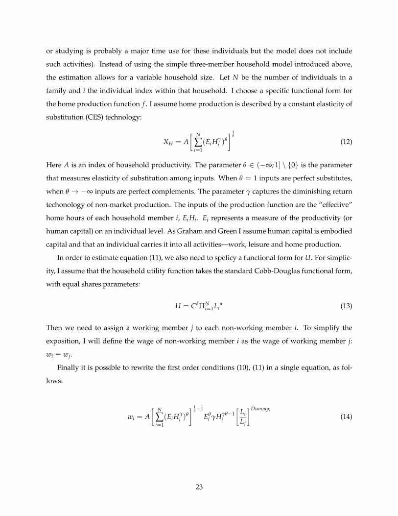
or studying is probably a major time use for these individuals but the model does not include

such activities). Instead of using the simple three-member household model introduced above,

the estimation allows for a variable household size. Let N be the number of individuals in a

family and i the individual index within that household. I choose a specific functional form for

the home production function f . I assume home production is described by a constant elasticity of

substitution (CES) technology:

XH = A[ N

∑i=1

(Ei Hγi )

θ

] 1θ

(12)

Here A is an index of household productivity. The parameter θ ∈ (−∞; 1] \ {0} is the parameter

that measures elasticity of substitution among inputs. When θ = 1 inputs are perfect substitutes,

when θ → −∞ inputs are perfect complements. The parameter γ captures the diminishing return

techonology of non-market production. The inputs of the production function are the “effective”

home hours of each household member i, Ei Hi. Ei represents a measure of the productivity (or

human capital) on an individual level. As Graham and Green I assume human capital is embodied

capital and that an individual carries it into all activities—work, leisure and home production.

In order to estimate equation (11), we also need to speficy a functional form for U. For simplic-

ity, I assume that the household utility function takes the standard Cobb-Douglas functional form,

with equal shares parameters:

U = CδΠNi=1Li

α (13)

Then we need to assign a working member j to each non-working member i. To simplify the

exposition, I will define the wage of non-working member i as the wage of working member j:

wi ≡ wj.

Finally it is possible to rewrite the first order conditions (10), (11) in a single equation, as fol-

lows:

wi = A[ N

∑i=1

(Ei Hγi )

θ

] 1θ−1

Eθi γHγθ−1

i

[Li

Lj

]Dummyi

(14)

23

where

Dummyi =

0 if individual i works

1 if individual i does not work(15)

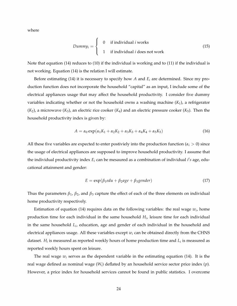
Note that equation (14) reduces to (10) if the individual is working and to (11) if the individual is

not working. Equation (14) is the relation I will estimate.

Before estimating (14) it is necessary to specify how A and Ei are determined. Since my pro-

duction function does not incorporate the household “capital” as an input, I include some of the

electrical appliances usage that may affect the household productivity. I consider five dummy

variables indicating whether or not the household owns a washing machine (K1), a refrigerator

(K2), a microwave (K3), an electric rice cooker (K4) and an electric pressure cooker (K5). Then the

household productivity index is given by:

A = α0 exp(α1K1 + α2K2 + α3K3 + α4K4 + α5K5) (16)

All these five variables are expected to enter postiviely into the production function (αi > 0) since

the usage of electrical appliances are supposed to improve household productivity. I assume that

the individual productivity index Ei can be mesaured as a combination of individual i′s age, edu-

cational attainment and gender:

E = exp(β1edu + β2age + β3gender) (17)

Thus the parameters β1, β2, and β3 capture the effect of each of the three elements on individual

home productivity respectively.

Estimation of equation (14) requires data on the following variables: the real wage wi, home

production time for each individual in the same household Hi, leisure time for each individual

in the same household Li, education, age and gender of each individual in the household and

electrical appliances usage. All these variables except wi can be obtained directly from the CHNS

dataset. Hi is measured as reported weekly hours of home production time and Li is measured as

reported weekly hours spent on leisure.

The real wage wi serves as the dependent variable in the estimating equation (14). It is the

real wage defined as nominal wage (Wi) deflated by an household service sector price index (p).

However, a price index for household services cannot be found in public statistics. I overcome

24

this problem by using the nominal wage Wi as the dependent variable. In this way, the price

index is treated as a parameter to be estimated, although it cannot be identified separately from

the constant α0 in the right-hand side of the estimating equation (14). This procedure does not

involve any loss of relevant information, since I am not interested in p itself and the purpose of the

estimation is to derive the monetary value of home output (pXH), not its real value.

I estimated equation (14) by non-linear least squares in STATA. Table 7 reports the estimation

results. The estimate of θ is highly significant, implying that the CES assumption fits well the actual

household production technology. The estimated θ is almost equal to one indicating a high degree

of substitutability among the effective home work hours of the household members. The estimate

of γ is positive and significantly close to one. Thus the marginal product of each individal is ap-

proximately constant . As we expected, all the general household productivity parameters have

positive signs except α2, which is not statistically significant. Usage of microwaves (α3) and elec-

tric rice cookers (α4) significantly improve household level productivity. Both education (β1) and

age (β2) have significant positive effect on each individual’s productivity at home. Surprisingly,

women have lower marginal productivity at home than men (gender is coded as 2 for female and

1 for male), although the coefficient is not significant12. Given the characteristics of a household,

these estimates can be used to compute the nominal value of home production as:

Vstructural = pα0e(α1K1+α2K2+α3K3+α4K4+α5K5)

[ N

∑i=1

(e(β1edui+β2agei+β3genderi)Hγi )

θ

] 1θ

(18)

I illustrate the result of this valuation method in the next section (see Table 9).

12The negative sign may come from the inability of the model to capture the gaps between male and female in bothhome hours and market wages. From (14), if there is a gap between male and female in wages, in order to equate thecondition with an inverse gap in home hours, the model has to yield a lower female home productivity. If we restrictour sample only to the retired individuals, to whom I assign the wage of the matched working individual in the family,the estimate of β3 is both positive and significant, at around 0.979.

25

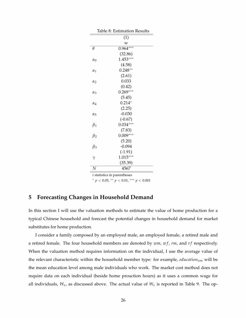
Table 8: Estimation Results(1)w

θ 0.964∗∗∗

(32.86)α0 1.453∗∗∗

(4.58)α1 0.248∗∗

(2.61)α2 0.033

(0.42)α3 0.269∗∗∗

(5.45)α4 0.214∗

(2.25)α5 -0.030

(-0.67)β1 0.034∗∗∗

(7.83)β2 0.009∗∗∗

(5.20)β3 -0.094

(-1.91)γ 1.015∗∗∗

(35.39)N 4567t statistics in parentheses∗ p < 0.05, ∗∗ p < 0.01, ∗∗∗ p < 0.001

5 Forecasting Changes in Household Demand

In this section I will use the valuation methods to estimate the value of home production for a

typical Chinese household and forecast the potential changes in household demand for market

substitutes for home production.

I consider a family composed by an employed male, an employed female, a retired male and

a retired female. The four household members are denoted by wm, w f , rm, and r f respectively.

When the valuation method requires information on the individual, I use the average value of

the relevant characteristic within the household member type: for example, educationwm will be

the mean education level among male individuals who work. The market cost method does not

require data on each individual (beside home prouction hours) as it uses a common wage for

all individuals, Wx, as discussed above. The actual value of Wx is reported in Table 9. The op-

26

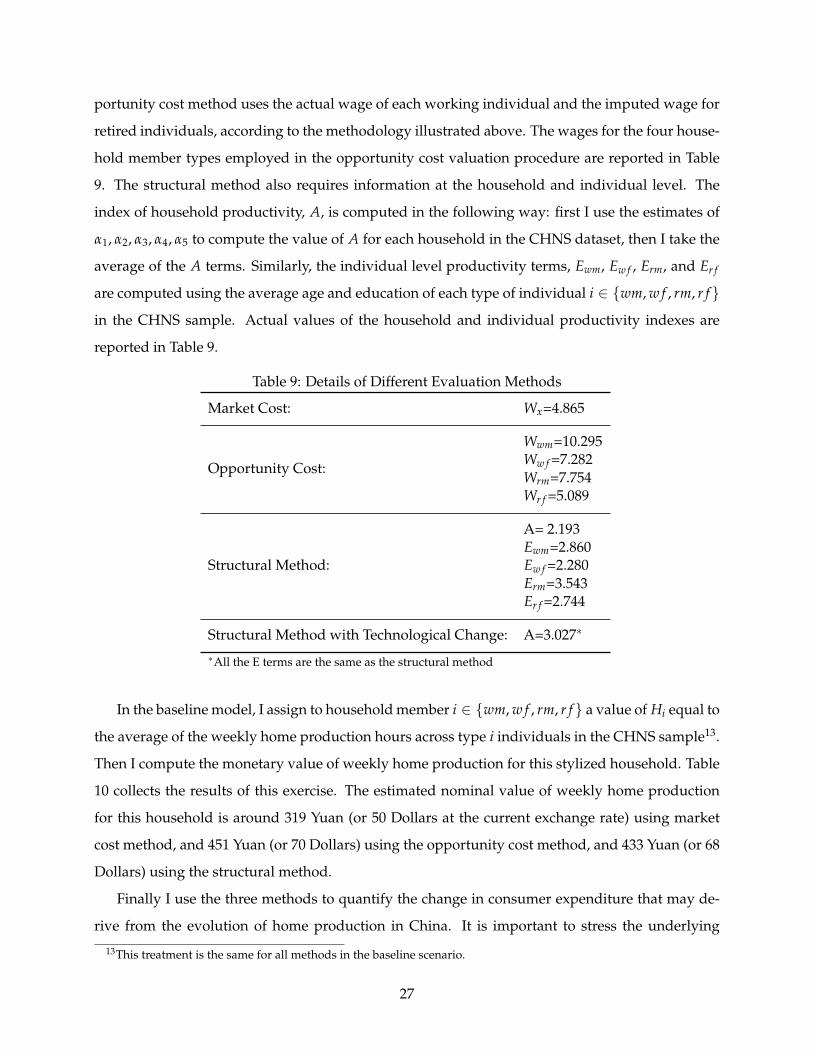
portunity cost method uses the actual wage of each working individual and the imputed wage for

retired individuals, according to the methodology illustrated above. The wages for the four house-

hold member types employed in the opportunity cost valuation procedure are reported in Table

9. The structural method also requires information at the household and individual level. The

index of household productivity, A, is computed in the following way: first I use the estimates of

α1, α2, α3, α4, α5 to compute the value of A for each household in the CHNS dataset, then I take the

average of the A terms. Similarly, the individual level productivity terms, Ewm, Ew f , Erm, and Er f

are computed using the average age and education of each type of individual i ∈ {wm, w f , rm, r f }

in the CHNS sample. Actual values of the household and individual productivity indexes are

reported in Table 9.

Table 9: Details of Different Evaluation Methods

Market Cost: Wx=4.865

Opportunity Cost:

Wwm=10.295Ww f =7.282Wrm=7.754Wr f =5.089

Structural Method:

A= 2.193Ewm=2.860Ew f =2.280Erm=3.543Er f =2.744

Structural Method with Technological Change: A=3.027∗

∗All the E terms are the same as the structural method

In the baseline model, I assign to household member i ∈ {wm, w f , rm, r f } a value of Hi equal to

the average of the weekly home production hours across type i individuals in the CHNS sample13.

Then I compute the monetary value of weekly home production for this stylized household. Table

10 collects the results of this exercise. The estimated nominal value of weekly home production

for this household is around 319 Yuan (or 50 Dollars at the current exchange rate) using market

cost method, and 451 Yuan (or 70 Dollars) using the opportunity cost method, and 433 Yuan (or 68

Dollars) using the structural method.

Finally I use the three methods to quantify the change in consumer expenditure that may de-

rive from the evolution of home production in China. It is important to stress the underlying

13This treatment is the same for all methods in the baseline scenario.

27

hypothesis: I assume that, as home work hours change, the total value of household consumption

is constant, so that a reduction in home production translates into an increase in demand for mar-

ket substitutes. While this assumption is clearly restrictive, it helps to focus on a specific channel

through which private demand may increase. Even though changes in home work hours are likely

to be correlated with many other changes in the economy, the effects on private demand could al-

ways be decomposed into an overall change in households’ consumption target and a reallocation

between home and market. Here I focus on the latter. Moreover, since the overall change in house-

holds’ consumpion target is likely to be positive in the medium run (i.e. an increase in private

consumption) my estimates are unlikely to overstate the potential gains in private demand and

rather provide a conservative lower bound.

In the scenario labelled “Convergence”, I estimate the level of home production that would

obtain if the same Chinese household of the baseline scenario allocated hours to home production

as an average American family. Thus, I set Hi (i ∈ {wm, w f , rm, r f }) equal to the average of the

weekly home production hours across type i individuals in the ATUS sample. The estimation is

based on the assumption that the elasticity of substitution, the household level and the individual

level productivity terms are all fixed. The results are summarized in table 1014. The value of home

production is expected to fall by around 157 Yuan per week according to the opportunity cost and

structural methods, or by 112 Yuan according to the market cost method. This implies that the

evolution of home production time in China can generate an equivalent increase in household ex-

penditure on household services: px∆XM = −px∆XH . The increase in demand is equivalent to

12% of household income using the opportunity cost and structural methods, or to 9% of house-

hold income according to the market cost method.

This estimate may overstate the actual potential gain in demand if the difference in Chinese-US

home work hours is due to differences in home production technologies instead of differences in

real wages. In other words, if the reduction in home work hours is due to the fact that households

can spend less time in housework while obtaining the same amount of home production, then

the reallocation of consumption to the market may be negligible. In order to account for this

possibility, I study another scenario, labelled “Appliances”, in which I use the structural model

but with a higher level of household productivity (a higher A term). Specifically, I set each one of

the elettrical appliances usage dummies K1, K2, K3, K4, K5 equal to one (instead of using the current

14I compute the nominal value of home production by using the same price index of household services employed inthe baseline scenario so that the two scenarios can be compared also in nominal terms.

28

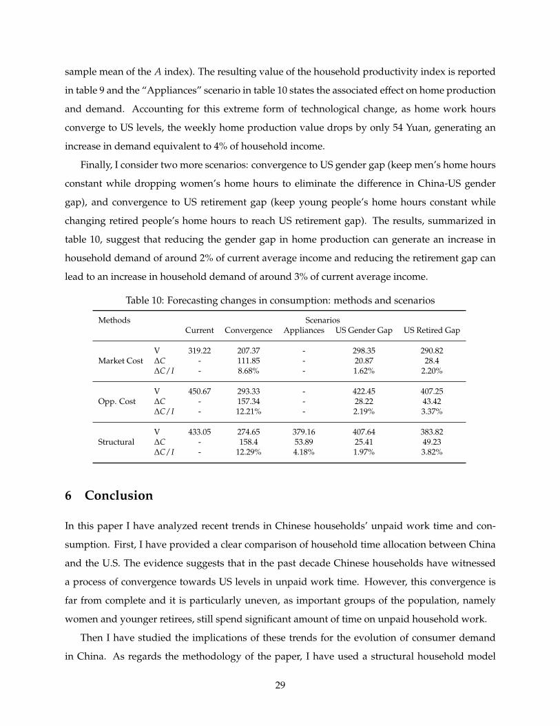
sample mean of the A index). The resulting value of the household productivity index is reported

in table 9 and the “Appliances” scenario in table 10 states the associated effect on home production

and demand. Accounting for this extreme form of technological change, as home work hours

converge to US levels, the weekly home production value drops by only 54 Yuan, generating an

increase in demand equivalent to 4% of household income.

Finally, I consider two more scenarios: convergence to US gender gap (keep men’s home hours

constant while dropping women’s home hours to eliminate the difference in China-US gender

gap), and convergence to US retirement gap (keep young people’s home hours constant while

changing retired people’s home hours to reach US retirement gap). The results, summarized in

table 10, suggest that reducing the gender gap in home production can generate an increase in

household demand of around 2% of current average income and reducing the retirement gap can

lead to an increase in household demand of around 3% of current average income.

Table 10: Forecasting changes in consumption: methods and scenarios

Methods ScenariosCurrent Convergence Appliances US Gender Gap US Retired Gap

Market CostV 319.22 207.37 - 298.35 290.82∆C - 111.85 - 20.87 28.4∆C/I - 8.68% - 1.62% 2.20%

Opp. CostV 450.67 293.33 - 422.45 407.25∆C - 157.34 - 28.22 43.42∆C/I - 12.21% - 2.19% 3.37%

StructuralV 433.05 274.65 379.16 407.64 383.82∆C - 158.4 53.89 25.41 49.23∆C/I - 12.29% 4.18% 1.97% 3.82%

6 Conclusion

In this paper I have analyzed recent trends in Chinese households’ unpaid work time and con-

sumption. First, I have provided a clear comparison of household time allocation between China

and the U.S. The evidence suggests that in the past decade Chinese households have witnessed

a process of convergence towards US levels in unpaid work time. However, this convergence is

far from complete and it is particularly uneven, as important groups of the population, namely

women and younger retirees, still spend significant amount of time on unpaid household work.

Then I have studied the implications of these trends for the evolution of consumer demand

in China. As regards the methodology of the paper, I have used a structural household model

29

that provides several advantages over more standard accounting methods, such as explicitly tak-

ing into consideration the contribution of retired household members and of electrical appliances.

The results of this study show that the value of home production that an average Chinese house-

hold generate is around 68 dollars a week, which is about 3300 dollars on an annual basis. As

the Chinese market economy expands, there will be more incentives for Chinese households to

substitute market activity for home production. The potential increase in household consumption

I estimate is significant, and equivalent to around 12% of current average household income in the

main scenario I consider, but I also present a number of alternative scenarios with more qualified

conclusions.

Such increase in household demand would play a significant role in driving the Chinese econ-

omy toward a more consumption-based and more balanced growth. While there is evidence of

trends in this direction, the transition will probably require active policies, from facilitating the

labor market participation of women and elderly people who are still productive, to guaranteeing

competition and lower prices in the market for household services.

30

7 References

Aguiar M., Hurst E.,“Lifecycle Prices and Production,” American Economic Review 97 (2007).

Becker, G. S., “A Theory of the Allocation fo Time,” The Economic Journal 75 (Sept., 1965).

Benhabib, J., R. Rogerson and R. Wright “Homework in Macroeconomics: Household Produc-

tion and Aggregate Fluctuations,” Journal of Political Economics 99 (Dec., 1991).

Eisner, R., “Extended Accounts for National Income and Product,” Journal of Economic Literature

26 (1988).

Graham, J. W. and C. A. Green, “Estimating the Parameters of a Household Production Func-

tion with Joint Products,” The Review of Economics and Statistics 66 (May, 1984).

Gronau, R., “Leisure, Home Production and Work – The Theory of the Allocation of Time

Revisited, ” Journal of Political Economy 85 (Dec., 1977).

Gronau, R., “Home Production – A Forgotten Industry, ” The Review of Economics and Statistics

62 (Aug., 1980).

Gronau, R., “Home Production – A Survey, ” Handbook of Labor Economics, Volume I, Chapter 4

(1986).

Guo, Kai, y Papa N’Diaye, “Determinants of China’s Private Consumption: An International

Perspective,” IMF Working Paper 10/93 (2010).

Hawrylyshyn, O., “The Value of Household Services: A Survey of Empirical Estimates,” Review

of Income and Wealth 22 (1976).

Kooreman, P. and Kapteyn, A., “A Disaggregated Analysis of the Allocation of Time within the

Household, ” Journal of Political Economics 95 (Apr., 1987)

Lee, Y.J. and Z. Xiao, “Children’s Support for Elderly Parents in Urban and Rural China: Results

From a National Survey,” Journal of Cross-Cultural Gerontology (1998) 13:39-62

Maurer-Fazio, M., R. Connelly, L. Chen, and L. Tang, “Child Care, Elderly, and Labor Force

Participation of Married Women in Urban China, 1982-2000,” Journal of Human Resources 46 (2):

261-94 (2011)

Parente, Stephen, Richard Rogerson, and Randall Wright, “Homework in Development Eco-

nomics,” Journal of Political Economy CVIII (2000), 680-687.

Ramey, V., “Time Spent in Home Production in the 20th Century United States: New Estimates

from Old Data,” Journal of Economic History, 69 (2009)

World Bank 1997. China 2020: Old Age Security and Pension Reform in China.

31