Forecasting Disconnected

Exchange Rates

Travis J. Berge

November 2011

RWP 11-12

November 2011

Forecasting disconnected exchange rates∗

Abstract

Catalyzed by the work of Meese and Rogoff (1983), a large literature has documented the inability ofempirical models to accurately forecast exchange rates out-of-sample. This paper extends the literature byintroducing an empirical strategy that endogenously builds forecast models from a broad set of conventionalexchange rate signals. The method is extremely flexible, allowing for potentially nonlinear models for eachcurrency and forecast horizon that evolve over time. Analysis of the models selected by the proceduresheds light on the erratic behavior of exchange rates and their apparent disconnect from macroeconomicfundamentals. In terms of forecast ability, the Meese-Rogoff result remains intact. At short horizons, themethod cannot outperform a random walk, although at longer horizons the method does outperform therandom walk null. These findings are found consistently across currencies and forecast evaluation methods.

• JEL: C4, C5, F31

• Keywords: Forecasting; exchange rates; classification; boosting.

Travis J. BergeFederal Reserve Bank of Kansas City1 Memorial AveKansas City, MO 64198Email: Travis.J.Berge@kc.frb.orgPhone: 816.881.2294

∗A portion of this manuscript was completed while visiting the Federal Reserve Bank of St. Louis, which I thank

for its generous hospitality. I also thank without implication Colin Cameron, Oscar Jorda, Chris Neely and Alan M.Taylor.

1 Introduction

Meese & Rogoff (1983) established that models of the exchange rate based on macroeconomic

fundamentals cannot produce forecasts that are consistently more accurate than a null random

walk model. While the literature has uncovered a modicum of evidence that connects exchange

rate movements to macroeconomic fundamentals,1 a very large body of empirical work has since

confirmed these findings using different fundamentals, currencies and forecast models so that it is

fair to say that fundamentals-based models do not convincingly outperform a random walk when

forecasting nominal exchange rates. For example, when concluding their comprehensive survey of

fundamentals-based models of the exchange rate, Cheung, Chinn & Pascual (2005) conclude that

“[no] model/specification [is] very successful. On the other hand, some models seem to do well at

certain horizons, for certain criteria.”

This paper employs a statistical method designed to incorporate two important observations

regarding the data generating process for nominal exchange rates. The first observation is the

striking feature that despite the foreign exchange market’s depth, liquidity and the sophistication

of the traders involved in the market, participants frequently change their views on the driving

forces behind the movement in the nominal exchange rate (Chen & Chinn 2001). The second

observation is the strong evidence for nonlinear movements in nominal exchange rates. Taken

together, these two observations—instability and nonlinearity—may account for the observation

that exchange rates appear to be disconnected from macroeconomic fundamentals. The fact that

exchange rates appear to be unstable motivates the use of a broad set of exchange rate signals

when forecasting exchange rates, allowing the forecast model to evolve through time. The method

used here endogenously selects a forecast model for a given currency and forecast horizon from a

menu of fundamentals that have been identified by the literature, including important drivers and

leaving out irrelevant ones. In addition, the method is flexible enough to take into account possible

nonlinearities that may be driving movements in the exchange rate. Nonlinear modeling has long

been an enticing potential solution to the Messe-Rogoff puzzle, albeit one that thus far has not

produced successful forecast models.

To be concrete, the algorithm searches over a menu of fundamentals previously identified by

the literature as determinants of the exchange rate, uncovering the signals that have the highest

correlation with previous movements in the exchange rate. The final model is chosen to be the one

that minimizes an information criterion so that the forecasting model is penalized for complexity.

In this way, as one estimates the model with a rolling-window, the method selects the drivers of the

1 It is not uncommon to find evidence of predictability, particularly at long forecast horizons. The classic citationis Mark (1995), who finds evidence that monetary aggregates do correlate with exchange rate movements, althoughFaust, Rogers & Wright (2003) note that this relationship appears to be present only during the sample periodused by Mark. More recently, Molodtsova & Papell (2009) tie exchange rate movements to interest rates instead,successfully forecasting exchange rates using signals derived from Taylor rules. Molodtsova & Papell (2010) documentthe performance of Taylor-rule based models through the recent financial crisis. Chen & Tsang (2009) use factors fromyield curves to successfully forecast at multiple forecast horizons. Engel, Mark & West (2008) argue for predictabilityat long horizons, and find that their factor-augmented model (Engel, Mark &West 2009) can forecast major currenciesat long horizons.

1

exchange rate and allows the covariates to vary across time in the impact they have on the exchange

rate. An important advantage of the method is that it makes explicit the tradeoff between bias and

variance of the model—the method produces forecast models that are biased, but it is precisely

this bias that may allow the model to produce accurate forecasts.2

The primary aim of the study is twofold. The initial analysis is focused on the empirical

approximation of the data generating process and the information content of the fundamentals

considered. Specifically, I ask whether the procedure can select the fundamentals most important

for exchange rate determination when producing in-sample forecasts. Although the in-sample

accuracy of the forecasting model is not interesting in and of itself, given the models selected to

produce the in-sample forecasts, I am able to explore questions regarding the instability of the

exchange rate model. For example, which fundamentals enter into the forecasting model for each

currency? Is there much “churning” in the data generating process—that is, once a fundamental

has entered the forecasting model at time t, how likely is it to be included at t+1? Do different

fundamentals matter when forecasting at different horizons? The paper then turns to the issue

of forecasting exchange rates out-of-sample. Although the literature on out-of-sample forecasting

is vast, the present paper adds to the literature by considering the method’s ability to select a

model able to forecast out-of-sample. At issue is not the forecast ability of a particular signal of

the exchange rate; instead, because the model considers a wide-range of covariates, at issue is the

method’s ability to ex ante include the fundamentals most important for forecasting.

To preview the results, the model selection technique produces forecasting models that differ for

each currency and at each horizon. At short horizons, the models include only a few fundamentals

that can loosely be described as ‘rules-of-thumb.’ The models forecasting at high frequencies are

very sparse and are not dissimilar to a random walk, reflecting the highly volatile nature of ex-

change rate movements at this frequency. Nevertheless, in-sample forecasts indicate that the model

selection procedure works well; at all of the forecast horizons considered the method outperforms

a random walk. The models that forecast at longer horizons include more fundamentals relative

to the short-horizon forecasts, though again unimportant signals are disregarded. There does ap-

pear to be an evolving relationship between economic fundamentals and exchange rate movements.

Out-of-sample, however, the method has trouble producing accurate forecasts and the results from

the forecasting exercise largely confirm the previous literature. High-frequency movements in nom-

inal exchange rates are difficult to forecast, although the method performs reasonably well when

forecasting at the longer horizons of six and 12 months. Regardless, the analysis nudges the lit-

erature in a new direction by making the argument that it is not a lack of information content in

fundamentals that is to blame for unsuccessful forecast accuracy but rather model misspecification.

2 For a recent discussion in the economics literature about forecasting and model overfit, see the discussion inCampbell & Thompson (2005), Goyal & Welch (2008) and Calhoun (2011).

2

2 Modeling the exchange rate

The primary objective is to link movements in nominal exchange rates to economic fundamentals

or other currency signals that may portend movements in the exchange rate. The model we wish

to estimate takes the generic form

∆het+h = F (θ, xt) + εt+h, (1)

where et denotes the log of the dollar price of foreign currency, ∆h represents the h-period differ-

ence operator, θ denotes a vector of model parameters and xt denotes a k-dimensional vector of

covariates. Equation 1 is written as general as possible so that it incorporates atypical models like

the ones implemented below. A more common expression for the forecast model is the linear model

∆het+h = xtβ + εt+h, (2)

where again xt is a matrix of k predictor variables and a constant.

2.1 Complications

An intrinsic problem for standard forecast models is that exchange rates are not well-behaved

relative to the data generating processes implied by forecasting models such as the one in equation

2. Recent papers that successfully forecast out-of-sample overcome this problem by estimating

models that essentially smooth this variability by taking averages over large quantities of data as a

way to approximate expectations for future macroeconomic fundamentals and therefore movements

in exchange rates. Engel et al. (2009), Chen & Tsang (2009) and Berge, Jorda & Taylor (2010) all

use some type of factor model in order to extract broad measures of market expectations for future

macroeconomic fundamentals.3

The method used here takes a slightly different approach designed to take into account two

peculiarities of exchange rate movements. First, the method directly addresses the empirical regu-

larity that model parameters in exchange rate models are unstable by performing model selection.

Rather than taking an average of a large number of macroeconomic variables and treating it as an

approximation to an underlying fundamental as is done by a factor model, the method explicitly

takes into account the fact that “some models seem to do well” (Cheung et al. 2005) at certain

points of time. When forecasting at each period and for each horizon, only those variables most

relevant for the forecast are included in the forecast model. Second and importantly, the frame-

work used here is able to employ nonlinear forecasting models. The nonlinear models address the

empirical regularity that exchange rate behavior appears to be nonlinear in nature.

3 Chen & Tsang (2009) and Berge et al. (2010) extract factors from relative yield curves, while Engel et al. (2009)derive factors from a cross-section of exchange rates, arguing that exchange rates themselves contain information thatis difficult to extract from macro fundamentals.

3

2.1.1 Parameter instability

A number of authors have noted that forecast models appear to exhibit unstable parameters and

that this parameter instability is a detriment to the model’s ability to forecast well. Survey ev-

idence from Chen & Chinn (2001) confirms that parameter instability is an important feature of

the foreign exchange market. The authors document that traders active in the foreign exchange

market frequently change the weight that they attach to particular fundamentals. Indeed, Meese &

Rogoff (1983) themselves speculated that parameter instability could be to blame for the failure of

fundamentals based models relative to the random walk null. Stock & Watson (1996) have argued

that parameter instability is a widespread phenomenon when modeling macroeconomic aggregates.

Theoretically, the parameter instability in the exchange rate market has been explained in

a number of different ways. Meese and Rogoff noted that instabilities could arise because of

changes in money demand functions or policy regimes. Bacchetta and van Wincoop (2004, 2009)

give the most compelling model describing how instabilities could arise by developing a rational

expectations model of the foreign exchange market. In the model, the true data generating process

of the exchange rate contains fundamentals that are both observed and unobserved by traders.

As the traders attempt to learn the parameters of a reduced-form model, the parameters become

unstable. This is because traders observe exchange rate movements caused by unobservable shocks,

and attach these correlations ex-post to observable fundamentals instead.

Empirical evidence of instabilities in exchange rate modeling is large and here I cover only a

handful of relevant papers. The regime-switching models of Engel & Hamilton (1990), Engel (1994)

and Dueker & Neely (2007) provide evidence of instabilities in exchange rate models. These papers

allow model parameters to follow a Markov process and find regime-switching behavior at both

low (Engel and Hamilton, Engel) and high (Dueker and Neely) frequencies for exchange rate data.

Such findings have led many forecasting modelers to incorporate time-varying parameters into fore-

casting models in an attempt to improve forecast ability. When Bacchetta, Beutler & van Wincoop

(2009) calibrate a model of exchange rate movements with time-varying coefficients, they conclude

incorporating time-varying parameters does not improve out-of-sample predictive performance of

the model. A paper that is directly related to this one is Sarno & Valente (2009), which finds

that fundamentals and the exchange rate are strongly related, but that the fundamental that best

explains movements in the exchange rate changes frequently and can differ across currencies. When

employing a predictive procedure that performs model selection, their method cannot consistently

outperform a random walk out-of-sample, a finding that they interpret as a call for an improved

model selection scheme.

2.1.2 Nonlinearity

Nonlinear movements in the exchange rate also undermine the performance of standard forecasting

models. There is compelling evidence, based on both theory and empirics, that suggests exchange

rates are nonlinearly related to fundamentals. Sarno, Valente & Leon (2006) argue that transaction

costs in the asset market produce a bound within which exchange rate speculation is not profitable,

4

producing nonlinear movements to the nominal exchange rate. Limits to arbitrage in the goods

market similarly produce nonlinear deviations from a purchasing power parity derived fundamental

value (Obstfeld & Taylor (1997); Taylor & Taylor (2004)). Other factors that produce nonlinear

behavior in the exchange rate include limits to speculation such as liquidity constraints, stop-

loss trading rules or margin calls. Speculative attacks on the exchange rate such as in Krugman

(1979) or Flood & Marion (1999) could similarly produce nonlinear movements, as can central bank

interventions (Dominguez 1998).

In practice, however, it is extremely difficult to take advantage of nonlinearities for forecasting

purposes. The models of Engel & Hamilton (1990), Engel (1994) and Dueker & Neely (2007) find

that exchange rates exhibit regime switching behavior, but the Markov process cannot anticipate

regime changes out-of-sample.4 Other authors that use nonlinear regression techniques to forecast

exchange rates include Diebold & Nason (1990) and Meese & Rose (1991). Both find that locally-

weighted regression techniques do not improve exchange rate forecasts beyond what can be achieved

with a linear model. Similarly, the neural networks of Qi & Wu (2003) are unable to outperform a

random walk when forecasting exchange rate movements.

2.2 The menu of fundamentals

An advantage of the method is that I do not have to take a strong stand regarding particular drivers

of exchange rates. Instead I rely on the empirical algorithm to select the best forecast model from

a wide range of exchange rate signals. The predictors that I consider derive from the following

models of the exchange rate.

1. Momentum. Momentum is a rule of thumb that states that the change in the exchange rate

is a linear extrapolation from last period’s change. Although it is not an economic model

per se, momentum gives the model a dynamic structure. Momentum is also a signal that

produces economically significant returns to many assets, including foreign currencies.5

2. Uncovered interest parity. UIP implies ∆het+h = ih,t− i∗h,t, where ih,t denotes the return to a

risk-free debt-instrument of maturity h and denominated in U.S. dollars and i∗h,t

denotes the

same for a debt instrument whose payoff is denominated in a foreign currency.6 Although a

strict adherence to UIP would impose the restriction that the coefficient associated with the

interest differential be equal to unity, from the prospective of a forecaster there is no reason

to impose this restriction.

3. Deviation from the real exchange rate. Purchasing power parity pins down a fundamental

4 Interestingly, Dueker & Neely (2007) find that although the Markov-process cannot outperform a random walk interms of squared-error loss, technical-trading rules derived from the fitted Markov-process are nevertheless profitable.

5 Recently, Berge et al. (2010), Burnside, Eichenbaum & Rebelo (2011), and Menkhoff, Sarno, Schmeling &Schrimpf (2011) have all identified momentum as a useful predictor of currency movements.

6 When forecasting at the one month horizon, the risk-free return is approximated by the one month LIBOR rate.At the 12 month horizon, 12 month LIBOR rates are used instead.

5

value towards which exchange rates ought to revert.7 In particular, let p denote the log

of U.S. CPI and p∗ the log of the foreign CPI. Deviations from the log of the long-run real-

exchange rate are defined as qt − qt, where qt = et + p∗t − pt and qt =

�t−1t=1 qt.

4. Nelson-Siegel yield curve signals. In an attempt to capture a market-based expectation of

future macroeconomic activity, I construct signals from the relative term structure of gov-

ernment debt. Specifically, the signals included in the forecasting model derive from the

parametric method of Nelson & Siegel (1987).8 Nelson-Siegel models of the yield curve are

parsimonious yet powerful—although they contain only three factors, they are flexible enough

to capture the changing shapes of yield curves. Nelson-Siegel yield curves are known to corre-

late highly with domestic macroeconomic variables (Diebold, Rudebusch and Aruoba, 2005;

Rudebusch and Wu, 2008), as well as exchange rate movements, (Chen and Tsang, 2009).

The three yield curve factors that result from Nelson-Siegel procedure lend themselves to in-

tuitive interpretations. The level factor Lt has a constant loading across the yield curve and

captures factors that shifts the relative yield curve, such as changes in inflation expectations.

The slope factor, St has a loading of 1 at maturity m = 0 that decreases monotonically to

zero as the maturity increases. St reflects the short-end of the relative yield curve and is

highly correlated with monetary policy responses. Ct is a factor that has its greatest loading

in the middle of the yield curve—it has a loading of 0 at m = 0 and at very long maturities.

In general, the L and S factors contribute the most marginal information to the forecasting

equations. As descriptions of the term structure, the Nelson-Siegel curves fit the data very

well, often achieving R2 values approaching unity. The curves I fit here are no exception,

often having R2 values of over 0.9.

5. Taylor rule signals. The final signals derive from the policy responses of the central banks.

Engel et al. (2008) and Molodtsova & Papell (2009) have found that Taylor rule fundamentals

contain information useful for out-of-sample forecasts of the exchange rate. These papers

presuppose that central banks follow a Taylor rule with interest rate smoothing. Following

Clarida, Gali & Gertler (1998), it is assumed that central banks set interest rates in response

to deviations in output and inflation from their full-employment rates, and that non-U.S.

central banks also include deviations from the real exchange rate in their reaction function.

Thus Taylor rule models imply that the output gap, inflation differential and real exchange

7 Even if the reversions happen slowly; see Taylor & Taylor (2004).

8 Nelson-Siegel signals are produced by estimating the following factor model of the relative yield curve:

imt − i∗mt = Lt + St

�1− e−λm

λm

�+ Ct

�1− e−λm

λm− e−λm

�(3)

where m denotes the maturity of the government debt instrument and λ is a parameter that controls the speed ofexponential decay that, following Nelson & Siegel (1987), I set to 0.0609. For each country-time pair, equation 3 isestimated using a cross-section of government debt of varying maturity length m = 3, 6, 12, 24, 36, 60, 84, and 120months.

6

rate deviations be included in the forecasting model.9 For a detailed derivation of how the

exchange rate depends on monetary policy, see Molodtsova & Papell (2009).

6. A constant. The model includes an intercept term, so that it nests a random-walk with drift.

To summarize, the method I use below will perform model selection from the nine signals of

the exchange rate based on the models above. Namely, the signals include: a momentum signal;

the interest rate differential; a real-exchange rate deviation; level, slope and curve signals from a

Nelson-Siegel yield curve; the output gap differential; the inflation rate differential; and an intercept

term ([∆het, ih,t − i∗h,t, qt − qt, Lt, St, Ct, zt − z

∗t ,πt − π

∗t ,1]). This list represents many indicators

that have been previously identified by the literature as successful predictors of nominal exchange

rates.

2.3 Data

I use exchange rate and economic data from nine countries (Australia, Canada, Germany10 , Japan,

Norway, New Zealand, Sweden, Switzerland and the UK) relative to the United States. The data

are at a monthly frequency and span the time period January 1986 - December 2008.11 End-

of-month nominal exchange rates, industrial production and consumer price indices are from the

IMF’s International Financial Statistics database.12 LIBOR data are from the British Banker’s

Association,13 and data on government debt yields are from Global Financial Data.14

2.4 Introduction to the method

The method I use to perform model selection—generically known as boosting—has its foundations

in two distinct literatures, machine learning and statistics. The algorithm originated in the ma-

9 Output gaps for each country are constructed using industrial production as a proxy for total output andare denoted zt and z∗t . Although there are many methods that one could use to obtain the cyclical component ofindustrial production, I detrend by taking 12-month log differences of observed industrial production. This simple,linear approach is advantageous for out-of-sample forecasts for several reasons. First, it does not require a two-sided smoother, which may introduce look-ahead bias into the forecasts. In addition, more sophisticated detrendingschemes, e.g., the Hodrick-Prescott filter, introduce additional dynamic elements into the cyclical component and aresensitive to the sample used to extract the cyclical component. Consequently, the estimated output gap of period twould change as the curves are re-estimated along with the rolling regressions or as more data is observed. Inflationrates in each country are also calculated as the 12-month log difference of the consumer price index, and are denotedwith πt and π∗

t for the US and foreign country respectively.

10 After 1999, Germany data are constructed with the USD/EUR exchange rate, which is converted into GermanDeutsche Marks using the value of 1.95583 DEM/EUR.

11 The exceptions are as follows. Swedish LIBOR data are not available until January of 1987. Due to a lack ofgovernment-issued debt, Nelson-Seigel curves cannot be estimated until January 1991 for Switzerland (see section 3).New Zealand lacks industrial production data for the first several years of the sample. Data for Canadian industrialproduction is not available until January 1995, so a total manufacturing index from Industry Canada (www.ic.gc.ca)from is substituted when necessary.

12 www.imfstatistics.org

13 www.bba.org.uk

14 www.globalfinancialdata.com

7

chine learning literature as a method for solving classification problems. The quintessential boosting

algorithm is Adaboost (Freund & Schapire 1997), which has been applied to a wide-range of clas-

sification problems within the machine learning literature, such as spam detection for email, facial

recognition algorithms and medical diagnosis (see, e.g., Ridgeway, 1999; Shapire & Singer, 2000;

Schapire, 2002, and the references therein). Friedman, Hastie & Tibshirani (2000) introduced the

algorithm to the statistics literature, recasting the mechanical Adaboost algorithm as a likelihood

maximization problem thus connecting boosting algorithms to classical statistical procedures (also

see Hastie, Tibshirani & Friedman (2001)). Giving boosting a likelihood maximization foundation

sparked its use in many other applications, since the algorithm could easily be applied to loss func-

tions appropriate to a variety of statistical problems. Friedman et al. (2000) showed that Adaboost

minimizes a loss function akin to a Bernoulli log-likelihood function in order to relate covariates

to binomial outcomes. But when one minimizes squared-error loss instead, the algorithm approxi-

mates linear regression. Similarly, one can minimize loss functions in order to approximate logistic

regression, Cox-Box models, or quantile regression.

The objective is to build the function F (x) in equation 1 while imposing as little structure as

possible on the data. Boosting begins by positing the functional form of the relationship between

the outcome and each individual covariate with very simple relationships known as weak leaners.

Weak learners can take many forms. In the simplest application used here I consider univariate

OLS regressions as the weak learners, however, they can also be non-linear or non-parametric. The

function F—known as the strong learner—is built by combining the weak learners iteratively. At

each iteration, only the best fitting weak learner is added to the forecast model and an information

criterion is calculated. The final model is chosen to be the model from the iteration that mini-

mizes the information criterion. In this way, it is possible that certain covariates are determined

to strongly impact the outcome are appropriately weighted in the forecast model. Others may be

receive little or no weight in the final model because they add no information or so little informa-

tion that the gain is outweighed by the penalty imposed on model complexity by the information

criterion.

3 Methodology

3.1 Forecast environment

Forecasts of observation t+ h, where h denotes forecast horizon, are produced by direct forecasts.

All forecasts considered here are made with rolling regressions with window size R. Let T denote

the total number of observations so that P, the number of forecasts made, is given by P ≡ T −R − h + 1. The first out-of-sample prediction is made for period R + h using observations of

{xt}t=1,...,R. Forecast evaluation is based on the P × 1 vector of out-of-sample predictive errors,

{�∆et+h −∆et+h}t=T−P+1,...,T .

8

3.2 Boosting as gradient descent

The objective is to estimate the function F : RK → R that minimizes the expected loss

F (x) ≡ argminF (x)

E [L(y, F (x))] (4)

where y ∈ R is the outcome, x is a k-dimensional vector of covariates, E is the usual expectations

operator and L denotes a user-specified loss function. F , the strong learner, is specified to be an

affine combination of weak learners and takes the form

F (x) =M�

m=1

γmf(θm, x), (5)

where the basis functions f are functions with parameters θm, and the γm’s describe how the weak

learners are combined.

Solving for F (x) in one fell swoop is difficult since it requires the numerical optimization of an

empirical version of (4),

min{γm,θm}

T�

t=1

L�yt,

M�

m=1

γmf(θm, xt)

�. (6)

Instead, boosting solves problem (4) in a stage-wise manner. The algorithm due to Friedman (2001)

is described below, and can be summarized as follows. The algorithm begins by initializing the

learner in order to compute an approximate gradient of the loss function. Step 2 fits the weak

learner to the current estimate of the gradient and step 3 chooses the step-size and descends the

function space. In step 4 we iterate on 2 and 3 until iteration M.

Functional Gradient Descent.

1. Initialize. Initialize the learner f0, and set F0 = f0(θ, x). One common method for initial-ization is to set f0 equal to the constant c that minimizes the empirical loss. Let m denoteiterations. Set m = 0.

2. Projection. Compute the negative gradient vector evaluated at the current estimate of F ,Fm.

ut = −∂L(F, yt)∂F

|F=Fm(xt)

, t = 1, ..., T

Produce the new weak learner fm+1(θ, x) by fitting the covariates {x1, x2, ..., xT } to thecurrent gradient vector {u1, u2, ..., uT }.

3. Update Fm. Update the estimate of F ,

Fm+1(.) = Fm(.) + ρfm+1(.)

Most algorithms simply use a constant but sufficiently small step-length. The literaturehas determined that ρ = 0.1 is a sensible shrinkage factor. Alternatively, one can solve an

9

additional minimization problem for the best step-size:

ρ = argminρ

T�

t=1

L(yt, Fm(xt) + ρfm+1(xt)).

4. Iterate. Increase m by one. Iterate on Steps 2 through 4 until m = M .

In the case described in section 2.2, the weak learner is univariate OLS and the algorithm

minimizes squared error loss. The final estimator, FM (x) =�

M

m=0 ρ�βκ

m, converges to the unique

least squares solution as M → ∞ (Buhlmann (2003)).

The two major tuning parameters, ρ and M , jointly determine the number of iterations required

by the algorithm in order to converge. It is common in the literature to set the shrinkage parameter

ρ to a sufficiently small number, although one can solve the additional minimization in (3) to find

the optimal step-size at each iteration of the algorithm. In general, small values of ρ are desirable

to avoid overfitting. The cost of a small ρ is purely computational since the algorithm will require

more iterations to achieve convergence. M , the number of iterations performed by the algorithm,

is responsible for preventing model overfit.15 In the applications below, M is chosen to minimize

an AIC criterion; i.e. M ≡ argminmAIC(m).16 An alternative method is to use cross-validation

techniques to find M, something I do not explore here.

The AIC has a unique minimum value, which is used to define the number of iterations in the

algorithm. Intuitively, this is due to diminishing marginal returns in the explanation of the variance

of the outcome variable as we add complexity to the model. The first few iterations add significant

information over the initial model and drastically improve the model’s fit—the AIC goes down as

σ2 decreases. But as the model complexity increases, the marginal gain in explanatory power may

be outweighed by the penalty to model complexity. As an example, figure 1 displays the AIC(m)

for the model that was used to predict the end-of-month Australian Dollar-U.S. Dollar exchange

rate in January 2000 as a function of the number of boosting iterations.17 Panel (a) displays

the AIC from the model used to produce one month ahead predictions; panel (b) displays the AIC

of the model fit to make a prediction at a horizon of 12 months instead. Both figures display

the convex shape described above and define a unique stopping parameter M. Note the significant

difference in the number of iterations used to produce the final model—the model that predicts

15 See (Ridgeway 1999) and (Buhlmann & Yu 2003) for more on boosting’s resistance to overfitting.

16 Specifically, the information criterion can be written as

AIC(m) = log(σ2) +1 + trace(Bm)/R

(1− trace(Bm) + 2)/R, (7)

where R indicates the number of observations used to fit the model, Bm is the hat-matrix of the boosted model atiteration m whose trace measures the degrees of freedom of the model, and σ2 is the estimated variance of the modelat iteration m.

17 The model is fit with univariate OLS weak learners and is set to minimize the L2 loss function.

10

one month ahead includes only 11 iterations of the algorithm, whereas the model that predicts 12

months ahead includes 1,000 iterations.

[Figure 1 about here.]

3.3 Forecast evaluation

Forecasts are evaluated using two distinct metrics. The first evaluates the predictive ability of a

model; i.e., the model’s ability to produce forecasts that are ‘close’ in value to the realized outcome.

The tests of forecast accuracy are implemented via the test statistic of Giacomini & White (2006)

and test for absolute prediction error and mean squared prediction error. The second class of test

statistics evaluate classification ability instead. Classification is a statistical problem distinct from

forecast error and is a natural metric to consider because identifying the direction of change of an

exchange rate is at the heart of a currency trader’s problem.

3.3.1 Predictive ability

To test the accuracy of the predictions produced by the fundamentals-based models, I rely on

methods in the vein of Diebold & Mariano (1995), West (1996) and Giacomini & White (2006). The

tests of Diebold & Mariano (1995) and West (1996) require knowledge of the true data generating

process and rely on the convergence of the parameters of the forecast model to their true values.

This requirement is clearly not met by the method used here. As a consequence, I instead rely on

the Giacomini & White (2006) tests of conditional predictive ability.

The Giacomini-White test (GW henceforth) assesses whether or not the loss associated with the

predictions from a prospective model are on average different than the losses from the null model.

Let Li

t+h(εt+h) be the loss function that evaluates the accuracy of the prediction of observation

t+h, where i ∈ {0, 1} denotes the model used to produce the forecast and εt+h ≡ ∆ei

t+h−∆et+h is

the forecast error. The test statistic can be written as:

GW1,0 =

∆L

σL/√P

→ N(0, 1),where (8)

∆L =1

P

T−h�

t=R

�L1t+h − L

0t+h

�; σ

2 =1

P

T−h�

t=R

�L1t+h − L

0t+h

�2

Tables report the P-value that results from testing the null hypothesis that the proposed model

produces errors that are on average not different from those of the null model.18 The loss functions

LiMAFE = |∆e

i

t+h −∆et+h|, i ∈ {0, 1} (9)

LiMSFE = (∆e

i

t+h −∆et+h)2, i ∈ {0, 1} (10)

18 P-values are obtained by regressing ∆L on a constant and testing whether the slope coefficient differs from zerousing Newey-West standard errors robust to heteroskedasticity and autocorrelation.

11

correspond to using the metrics of absolute forecast error and squared forecast error to test for

forecast accuracy.

3.3.2 Classification ability

Classification ability has emerged in the exchange rate forecasting literature as a natural alternative

measure for forecast evaluation. Tests of the accuracy of point-forecasts rely on the specification

of a loss function for evaluation. Since a forecast model is only an approximation to the true data

generating process, different loss functions will result in different models and therefore potentially

different conclusions about model accuracy (Hand & Vinciotti 2003). As an alternative, testing

the classification ability of a model is a problem statistically distinct from testing forecast accu-

racy. A model focused on classification doesn’t necessarily require a point forecast. Instead, one

can think of the classification model as partitioning the covariate-space into disjoint regions. As

a consequence, the optimal classification model is not unique since there are many functions that

can partition the covariate-space into the same regions (Elliott & Lieli 2009). Finally, in terms

of economic significance, traders and policy makers may be interested in forecasts as classification

mechanisms. For example, zero net-profit investments such as the carry trade are primarily clas-

sification problems—get the direction of change correct and profits are guaranteed. Cheung et al.

(2005) note that some empirical exchange rate models have classification ability even if the forecasts

are not significantly more accurate than a random walk in terms of mean squared error. Dueker &

Neely (2007) also provide a model that has classification ability despite unsuccessful mean squared

error forecast ability.

For these reasons, consider the problem of classifying the object dt+h ∈ {−1, 1}, where dt+h is

defined as the sign of ∆het+h. The classifier, dt+h, takes the form dt+h = sign(yt+h − c) for some

threshold value c and some signal y. The model that produces yt+h is most likely an estimate

of the conditional expectation of ∆het+h, but it need not be and can take many other forms, for

example, an estimate of the conditional probability of a movement in a particular direction or a

simple index.

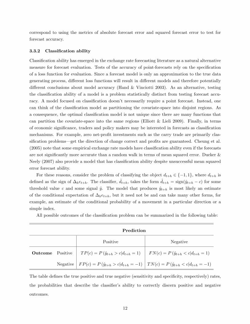
All possible outcomes of the classification problem can be summarized in the following table:

Prediction

Positive Negative

Outcome Positive TP (c) = P (yt+h > c|dt+h = 1) FN(c) = P (yt+h < c|dt+h = 1)

Negative FP (c) = P (yt+h > c|dt+h = −1) TN(c) = P (yt+h < c|dt+h = −1)

The table defines the true positive and true negative (sensitivity and specificity, respectively) rates,

the probabilities that describe the classifier’s ability to correctly discern positive and negative

outcomes.

12

The table above makes clear that both the true positive rate and true negative rate depend

on the choice of the threshold value c. As c is varied from −∞ to ∞ and treating TN(c) as the

abscissa, a curve is traced out in {TN(c), TP (c)} space that describes the classification ability of

the model. Berge et al. (2010) denote this curve as the Correct Classification Frontier,19 and the

area underneath this curve gives a parsimonious summary of the classification ability of a given

model. The statistic, known as the AUC, has a lower bound of 0.5 and an upper bound of 1. For

inferential purposes, standard errors are found with the bootstrap.20

The AUC statistic is also intimately related to the well-known Kolmogorov-Smirnov (KS )

statistic (Kolmogorov, 1933; Smirnov, 1939). Specifically, the KS statistic is the maximum distance

between the 45o line and the Correct Classification Frontier. The statistic is of particular interest

because it defines the point on the Correct Classification Frontier that would maximize the utility

of a forecaster who weighs correct and incorrect classifications equally when the outcome has equal

probability. The KS statistic can be shown to be

KS = maxc

|TP (c) + TN(c)− 1|

Since a coin-toss classifier has by definition a true positive and true negative rate of 0.5 for any

threshold value c, KS ∈ (0, 1) where a coin-toss classifier achieves a value of 0 and a perfect

classifier has a value of 1. For inferential purposes, the test statistic is known to be distributed

as a Brownian Bridge,21 although again in the application here the standard errors are from the

bootstrap.

One important advantage of these test statistics over other measures of classification ability is

19 The statistics originate from the receiver operating characteristic (ROC) curve, which I do not describe in detailhere; see Pepe (2003) for an extensive introduction. Within the economics literature, Berge & Jorda (2011) applyROC curves to the problem of classifying business cycles. Jorda & Taylor (2009), Berge et al. (2010) and Jorda &Taylor (2011) use ROC curves to evaluate models used to predict excess returns of zero-sum trading opportunities.

20 For details, see Jorda & Taylor (2011). However, Hsieh & Turnbull (1996) show that

√P��AUC − 0.5

�→ N(0,σ2), (11)

so that the statistic has a Gaussian distribution in large samples, and Hanley & McNeil (1982) provide a formula forthe estimation of the variance of AUC.

21 Namely, �P (1)P (−1)

PKS → sup

t|B(t)|,

where P denotes the number of forecasts made, P (1) is the number of observations where dt = 1, and P (−1) is thenumber when dt = −1.

13

that one can also instruct weighted versions of the AUC and KS statistics. In particular, weight

each observation by its contribution to the total movement of the exchange rate in one direction or

the other:

wi =yt

B∗ for i = 1, ..., P (1), and

wj =yt

C∗ for j = 1, ..., P (−1)

where B∗ =

�dt=1 yt, C

∗ =�

dt=−1 yt, and P(i) denotes the number of observations where dt = i.

This weighting scheme reflects the fact that from the point of view of a practitioner, a preferred

classification model would be the one that classifies large movements of the exchange rate relative

to an alternative model that correctly classifies small changes but misses the crashes. The em-

pirical distributions of the weighted classifiers define alternative statistics with which to measure

classification ability. The weighted versions of the AUC and KS statistics are denoted with an

asterisk.

4 Do fundamentals matter for the exchange rate?

Prior to undertaking a purely out-of-sample forecasting exercise, I first explore the results of the

model selection done by boosting the exchange rate signals described in section 2. Specifically, I

explore model selection within the context of producing in-sample forecasts of the exchange rate

at horizons of one, six and twelve months. In-sample forecasts are used since I am interested in

whether the method can select a useful model for the exchange rate when given the knowledge of

the realizations of future values of covariates. That is, I want to separate the issue of information

content in the signals from the issue of model selection out-of-sample. Conditional on the exchange

rate signals containing information useful for forecasting, the next section will examine the method’s

ability to forecast within the context of a standard out-of-sample exercise.

4.1 A linear model

I apply the functional gradient descent algorithm to the following loss function:

L(yt+h, F (xt)) =1

2[yt+h − F (xt)]

2, (12)

14

with yt+h ≡ ∆het+h and F (x) as defined in equation 5.22 The final model is an affine basis of the

elements of x, where xt = [1,∆het, ih,t − i∗h,t, qt − qt, Lt, St, Ct, zt − z

∗t ,πt − π

∗t ], the fundamentals

described in section 2. It is straightforward to show that the F∗(x) that minimizes (12) estimates

the expected value of yt+h; i.e., the model estimates a conditional mean.

At each iteration m the weak learner is defined as follows:

fm(x) = xκβκ

, where

�βk

=

�T

t=1 xkt ut�

T

t=1(xkt )

2, and (13)

κ = argmink

T�

t=1

(ut − xkt β

k

)2

so that the weak learner is component-wise least-squares regression. At each iteration we restrict

the evolution of the vector of slope coefficients, β as previously described. The boosted model at

step m is Fm(X) = X(βm−1 + ρβκm), where β

κm is a k × 1 matrix with zeros in every entry except

for the variable xκ, βm−1 is the vector of slope coefficients from the previous iteration, and X is

a R × k matrix of data. An information criterion is used to select the number of iterations of the

algorithm.

It is accepted that empirical models can explain movements of the exchange rate in-sample, so

we are not interested in the in-sample forecast ability of the method per se. But as a check on the

method’s ability to choose a model of the exchange rate and for completeness, table 1 displays the

results from the in-sample predictions of the models described by equations 12 and 13. Forecasts

are generated from models estimated using a rolling window of length 96 months, where since the

forecasts are in-sample, a forecast of period t+h is generated from a model estimated with covariates

through period t+h. All observations after the initial 96 are used for predictive purposes, so the

number of observations for each country may be different due to data availability.23 The table

is divided into three parts, one for each forecast horizon. The columns that display the P-values

for the Giacomini-White tests using mean absolute forecast error and mean squared forecast error

are labeled MAFE and MSFE, respectively. The next four columns display the unweighted and

22 The boosting algorithm associated the loss function in (12) has been denoted L2Boosting (Buhlmann & Yu 2003).The gradient vector of the loss function in (12) is the residual vector from an OLS regression (see step (2) of thefunctional gradient descent algorithm). Thus boosting with the L2 loss function is simply iterated least squares.

23 This is especially true for forecasts at the six month horizon. New Zealand, for example, does not have Liborrates or issue government debt at a six-month tenor and therefore I do not forecast the NZD at this forecast horizon.

15

direction-of-change weighted AUC and KS test statistics.

[Table 1 about here.]

The in-sample performance of the method is indeed impressive. In terms of forecast accuracy as

measured by the Giacomini-White statistics, the method produces forecasts that are more accurate

than those from a random walk for a majority of the countries at horizons of one and twelve months.

At the horizon of six months, the method produces forecasts more accurate than a random walk for

only three of the eight countries in the sample. However, classification ability is impressive across

all forecast horizons, as indicated by the AUC and AUC∗ statistics that are consistently greater

than 0.5, and the KS and KS∗ statistics that are consistently greater then 0.

4.2 What do the models look like?

That the method is able to produce models that can accurately forecast exchange rates in-sample

is reassuring, because it indicates that the method is able to sort through the signals fed into the

algorithm in order to produce a model that is on target. But how is this being accomplished? What

do the models being selected look like?

Figure 1 displays the in-sample linear forecast of the h-period ahead change in the log nominal

exchange rate, as well as its realized value. To keep things concise, I display the figures only for

the Australian Dollar, Japanese Yen and British Pound. These currencies were chosen because

the in-sample forecasts display different patterns of forecast ability (see table 1). Immediately it is

clear that the exchange rate is much more volatile then its conditional expectation from the forecast

model. This in and of itself is not surprising. However, notice that the variability of the conditional

expectation is increasing in the forecast horizon. The actual exchange rate is extremely noisy at

high frequencies, and the model selection procedure chooses a model that is similar to a random

walk forecast. At longer horizons, we can see that the forecasts begin to track the changes in the

exchange rate (albeit with varying degrees of success), as opposed to choosing a model similar to a

random walk.

[Figure 1 about here.]

Table 2 gives further insight why this is the case. Table 2 displays summary statistics that

describe the number of regressors included in the forecast model for each country and forecast

16

horizon, averaged across all forecasting models estimated via the rolling window. Models that

forecast at very high frequencies tend to include relatively few regressors—only about three on

average. In contrast, the models that forecast at medium and long horizons include more regressors,

around seven of the nine available. This disparity is a result of the number of iterations used to

fit the model, which itself depends on the volatility of exchange rate changes. When forecasting at

medium and long horizons, the exchange rate data itself is smoothed and tends to have a higher

correlation with the fundamentals considered here. This can also be seen in the number of iterations

that minimizes the AIC criterion. For example, for forecasts fit to the AUD/USD exchange rate

and forecasting one-month ahead, the method minimizes the AIC criterion is minimized in less

then 40 iterations of the algorithm. When forecasting 12 months ahead, the number of iterations

needed to minimize the algorithm nears 3,000 on average.

[Table 2 about here.]

Figures 2-4 are an alternative visual representation of the results given in table 2. The figures

display the frequency with which any given exchange rate signal is chosen by the method across all

iterations.24 Consider the results displayed in figure 2, the models forecasting one month ahead.

It appears that there exists a group of exchange rate signals that, for forecasts at short horizons,

the method treats as ‘rules of thumb.’ The model that forecasts the Swiss Franc relies on only one

signal—the relative slope of the yield curve—for large periods of time. Other currencies heavily

involved in the carry trade also seem to rely on signals coming from the yield curve. The model

for the Japanese Yen displays a pattern similar to the Swiss Franc, while models for the Australian

and New Zealand Dollar tend to rely on the level of the yield curve instead. Momentum is another

signal that seems to enter into these short-run forecasts. But recall that the number of iterations

for these models is small. As a consequence the estimated model coefficients do not approach

their OLS equivalent, it is the fact that these slope coefficients are ‘shrunken’ that produces the

low-variance forecasts seen in figure 1.

24 Specifically, for each covariate k, let ψkt denote the selection frequency, where

ψkt =

1M

M�

m=0

I(k = κ); (14)

κ = argmink

�

t

(ut − fk(xkt ))

2.

17

[Figure 2 about here.]

[Figure 3 about here.]

[Figure 4 about here.]

At longer horizons as seen in figures 3 and 4, the exchange rate models appear to be more

stable, although still subject to changes in regime. It is clear that more variables are included in

each forecast model, although again since the algorithm stops prior to convergence, the estimated

coefficients do not necessarily approach their OLS equivalent. Although ‘instabilities’ are often

blamed for the lack of forecast ability for models of the exchange rate, the term is generally not

precisely defined,25 and it is not clear just how unstable we should expect these models to be.

Given that the model is fit with a rolling window, models that forecast t+h and t+h+1 ought to

be very similar. Given the relatively large window size (96 observations) it is not surprising that

there seems to be persistence in whether or not each covariate enters the final forecast model. That

new fundamentals seem to enter and exit the forecast model is consistent with the ‘scapegoat’ story

of Bacchetta & van Wincoop (2004). Sarno & Valente (2009) use a different approach for model

selection and also find that all the regressors they consider have important explanatory power.

In contrast to the findings here, however, Sarno & Valente (2009) find that no one covariate is

included in the ‘best’ forecast model for long periods of time, although Sarno & Valente forecast

only one-quarter ahead for all exchange rates.

Table 3 approaches the problem from a slightly different angle but largely confirms the inter-

pretation given to figures 3 and 4. Specifically, the table considers for each covariate a binomial

variable that defines whether or not a particular covariate is included in the model or not.26 The

table displays, for each country and forecast horizon, the unconditional frequency with which a

particular covariate is included in the forecast model. The table also gives the number of inclusion

spells for each individual covariate, and the average duration of those spells. The top panel of

countries gives the forecasts for one-month ahead changes in the exchange rate, the middle for

six-month ahead changes, and the bottom for the models forecasting one year ahead changes. For

25 Giacomini & Rossi (2009) is the exception.

26 Specifically the variable, I(ψh,k,t �= 0), where I(A) is the indicator function that takes on value of one whenevent A is true, and takes the value of zero otherwise.

18

example, focusing on the two components of the Taylor rule—inflation differentials and output

gap differentials—we see that the frequency with which these covariates are included in the model

increases as the forecast horizon increases. When forecasting the Australian dollar, the inclusion

frequencies for the inflation differential increase from 40 percent for one-month ahead forecasts to

94 and 100 percent for six and 12 month ahead forecasts. The inclusion frequencies for the output

gap differential follows a similar pattern, increasing from 33 percent (9 spells with an average du-

ration of 6 months per spell) to 88 percent for six month ahead forecasts and 95 percent for models

forecasting 12 months ahead.

In general, the longer the forecast horizon of the model, covariates are included more frequently,

and we observe fewer spells of inclusion that have a longer average duration. Qualitatively, one can

begin to see a picture where there are ‘short-term’ signals that may drive any particular exchange

rate for short periods of time and have short durations—for example, momentum—and more ‘long-

term’ fundamental drivers of exchange rates—for example, deviations from a real exchange rate and

output gap differentials—that have long durations and are often included in the forecast model,

especially at long horizons.

The analysis comes with an important caveat. Namely, that what is measured in figures 2-4

and table 3 is an “extensive margin” of the contribution of each covariate to the forecast model.

That is, what is being measured in table 3 is a binary indicator: the covariate was included in the

model or it was not. But because the boosted estimates of the model parameters are not their

OLS equivalent, the table does not necessarily give information about how important any given

covariate is when explaining the variation in exchange rate movements. The results are nevertheless

revealing. They speak to the degree to which forecast model are misspecified—a standard linear

forecast model would have each covariate included all the time and would include only a subset of

covariates. The results presented here indicate that this is a reasonable specification for forecast

models of long horizons, but is much less reasonable for short-horizon forecasts.

[Table 3 about here.]

4.3 Summary

This section presented a method to perform model selection and produce forecasts of nominal

exchange rates. The method makes explicit the bias-variance tradeoff that all econometric models

19

face when building models. At high frequencies and when the data is particularly volatile, imposing

OLS-estimated model parameters may lead to models that are unbiased but that will give volatile

and inaccurate forecasts. In contrast, the method recognizes that at short horizons exchange rates

are volatile and consequently it disregards much of the information contained in the covariates

considered. The method produces models that are biased but exhibit a low variance.

The results presented in table 1 confirm that the method is able to weight each covariate properly

when given realized data. When given realized data and judged by the squared-error metric, the

method can outperform a random walk model for 7 of the 9 countries considered. The question of

whether the method can perform out-of-sample as well remains. The next section addresses this

by examining the method’s ability to forecast out-of-sample.

5 Out-of-sample forecast performance

5.1 Performance of the linear model

The previous section analyzed whether the method is able to select a useful model of the exchange

rate when given the realized data. The more interesting and important issue is of course whether

the method can produce accurate out-of-sample forecasts of the nominal exchange rate. Table 4

describes the performance of the model defined by equations 12 and 13 in the previous section.

[Table 4 about here.]

Going from in-sample to out-of-sample forecasts makes a dramatic difference in the forecast

ability of the method. When forecasting at very short horizons and considering forecast error, the

method is unable to outperform a random walk model for any of the currencies considered. The

classification ability of the method is similarly unimpressive at short horizons—the method shows

consistent superior classification ability for only three of the nine currencies.

Unsurprisingly, as the forecast horizon becomes longer, the out-of-sample accuracy of the fore-

casts increases. That models built on economic fundamentals can provide accurate forecasts at long

horizons is well-known (Meese & Rogoff (1983); Mark (1995); Engel, Mark & West (2007)). When

forecasting at six months, the only currency with significant Giacomini-White test statistics is for

the Euro (German Mark) - U.S. dollar exchange rate. However, we do see that the forecast models

begin to display classification ability. For seven of the eight available currencies, the method can

20

consistently outperform a random walk in terms of forecast ability. It is when forecasting at 12

months that the forecast models have the most, though still modest, success. When judging by

squared-error metric, the model produces accurate forecasts for four of the nine currencies consid-

ered. The classification ability of the method is very good at this forecast horizon, with unweighted

AUCs generally between 0.70 and 0.90 and weighted AUCs around 0.80.

5.1.1 Exploring forecast breakdowns

Comparing the performance between the in-sample and out-of-sample models of the exchange rate

is revealing. The only difference between the two models is the information set used to fit the

models; the in-sample models include the h additional observations unobservable to a forecaster

in real-time. That the forecast ability of the models are so drastically different seems to imply

that the lack of forecast ability may be due to the method’s inability to perform model selection

out-of-sample rather than the predictive content contained in the fundamentals.

A simple way to investigate the cause of the forecast breakdown, and recalling the discussion

in section 4.2, table 5 reports the estimated coefficients from the regression

ψOOS

h,k,t = α+ βh,kψIS

h,k,t + εt (15)

where ψh,k,t is as defined in equation 14 and gives the frequency that a particular covariate k is

selected by the boosting method across all iterations performed at horizon h and time t. In the

interest of space and readability, regressions are reported as pooled across countries with standard

errors clustered on country.

These regressions test the ability of the out-of-sample model to select the proper covariates for

inclusion in the final boosted model, using the in-sample selections as the “gold standard.” A model

selection method able to replicate the in-sample selections would produce an intercept equal to zero

and a slope coefficient of unity, which is tested by the F-statistic in column 2 under each forecast

horizon. Columns 3 and 4 for each panel display the point estimates for the intercept and slope

coefficients, respectively. These restrictions are clearly rejected for each model covariate and for

each forecast horizon. That each slope estimate is less than one reflects the amount of “churning”

in the covariates selected by each model. Interestingly, although the forecast performance of the

models increases with the forecast horizon, there is little discernible pattern comparing the results

21

from this simple regression across forecast horizons. One may expect to see α approaching zero

and β approaching one as the forecast horizon becomes larger, but this does not appear to be the

case.

[Table 5 about here.]

Table 6 displays an alternative statistic to the one displayed in table 5. Instead of regressing the

fraction of iterations that pick up a particular covariate, the table instead explores the binomial

defined by whether or not a particular covariate was included in the forecast model, regardless

of weight. Specifically, the table displays the AUC statistic achieved when the indicator for the

in-sample model is used to explain the inclusion of covariates in the out-of-sample model. Recall

that the AUC statistic has a minimum value of 0.5 and a maximum value of 1.0, so an AUC

statistic that is close is to 1 indicates that the out-of-sample model includes a particular covariate

when forecasting the same period as the in-sample model. Qualitatively, the results displayed in

table 6 corroborate those in table 5, indicating that for no covariate does the out-of-sample model

approach the same performance of the in-sample model. For no covariate and forecast horizon pair

does the statistic approach one. Interestingly, the performance of the statistic across covariates is

surprisingly similar.

[Table 6 about here.]

5.2 A nonlinear model

Although modeling the exchange rate with a linear function is mathematically convenient, as pre-

viously discussed there is strong theoretical and empirical evidence suggesting that a nonlinear

model may be a more realistic modeling assumption. I introduce nonlinearity into the models

by using cubic smoothing splines as weak learners. Smoothing splines are an extremely flexible,

non-parametric modeling technique. Specifically, the nonlinear weak learners take the form of the

smoothing splines of Eilers & Marx (1996). For each covariate k, the spline minimizes the sum of

squared error:

PSSE(fk,λ) =

T�

t=1

[yt − fk(xt)]

2 + λ

�[fk��(z)]2dz (16)

with a smoothing parameter λ that penalizes functions with a large second derivative. Splines have

many features that make them attractive as weak learners in the boosting algorithm. In contrast to

22

the non-parametric regression techniques that have been utilized in much of the previous literature

(nearest-neighbor regression), smoothing splines are global in nature. They are also computation-

ally efficient and are easily implemented since they are essentially extensions of generalized linear

models.27

Incorporating smoothing splines into the boosting algorithm is straightforward. We again take

the approach of choosing at each iteration m the covariate that best minimizes the empirical loss

at that iteration. Let fkm be the smoothing spline fit to indicator k at iteration m. Then at each

iteration, the model will choose the spline that minimizes the sum of squared errors of the overall

fit of the model; i.e.,

fm(x) = fκ(x)

fk(x) = argmin

f(x)

�PSSE(f,λ, xk)

�(18)

κ = argmink

T�

t=1

(ut − fk(xt))

2

As before, the number of boosting iterations M will be chosen to be the one that minimizes the

AIC of the final boosted model.

The flexibility of the nonlinear model is a double-edged sword—while the models may fit well

in-sample,28 the danger is that the models will overfit when producing out-of-sample forecasts.

Moreover, we still require the method to perform model selection ex-ante. The out-of-sample

forecast ability of the model described by equation 18 is displayed in table 7. At short horizons

the model with smoothing splines is unable to overcome these obstacles. For no country is the

GW test statistically significant for both loss functions (indeed, in some cases the random walk

outperforms the boosted model!). In terms of classification ability, the smoothing spline model

27 I refer the reader to Eilers & Marx (1996) for details on the splines used here but briefly describe the method.Each spline consists of fitting high-order polynomials to the data. Penalizing the integral over the second derivativeof the function fk as in 16 is computationally very demanding. Instead Eilers & Marx approximate the penalty termby constraining the difference in parameter values of the spline in neighboring regions of the data. Estimation of themodel parameters can be transformed into a modified regression equation

β = (B�B + λD�D)−1B�y (17)

where B is a basis matrix describing the polynomials and D is a difference matrix that approximates the penaltyover the integral. Buhlmann & Yu (2003) have explored boosting with smoothing spline weak learners and find thatsetting λ = 4 is a reasonable setting for this parameter.

28 In the interest of conciseness I do not display the in-sample forecasts from the nonlinear model. The results fromthe exercise are very impressive, with the method easily outperforming a random walk, especially at longer horizons.

23

performs well for a few currencies, but the performance is not comprehensive. For many of the

currencies, the nonlinear boosted model is outperformed by the linear boosted model, indicating

that out-of-sample, the nonlinear model may be overfitting the data.

At longer horizons, however, the story is quite different as the nonlinear boosted model performs

extremely well. Consider first the results when forecasting six months ahead. For five of the

eight available currencies, the Giacomini-White test statistics are highly significant for both loss

functions, indicating that the model is indeed outperforming the random walk null. In addition,

we see that the models exhibit consistent classification ability. The results when forecasting one-

year ahead are similarly impressive. The P-values of the Giacomini-White test statistics are highly

significant. Many of the unweighted AUCs exceed 0.9 and in some cases the weighted AUCs

approach unity, indicating that the model achieves near-perfect weighted classification ability.

[Table 7 about here.]

The results of the nonlinear boosted model are impressive and constitute a unique contribution

to the vast empirical literature on nominal exchange rate prediction. Taken as a whole, the results

suggest that nonlinearities play an important role in exchange rate determination even at long

horizons. When producing out-of-sample predictions at short horizons, the nonlinear models seem

to overfit the noisy short-horizon data and are unable to outperform a random walk. However,

the model is able to exploit the relatively smooth data when forecasting one-year ahead. Whereas

the majority of the previous literature have mixed forecasting ability at this horizon, the boosted

model produces uniformly accurate predictions of the exchange rate, particularly when considering

the lower hurdle of classification.

5.3 Boosting for classification

The motivation behind the use of the L2 loss function in the analysis above is that the model

estimates the expected change of the exchange rate. But as the previous sections have shown, the

classification ability of a model provides a useful alternative on which to judge model performance.

From the perspective of a practitioner, knowing a model can classify the movement of an exchange

rate, even if its estimate of the point-value of that change is less reliable, may be useful information.

Moreover, classification ability is a fundamentally different metric on which to judge model perfor-

mance, and that it is a metric that directly connects to the profitability of speculation based on

24

model forecasts (Jorda & Taylor 2010). The literature focused on forecasting macroeconomic ag-

gregates has also emphasized the use of classification and asymmetric loss functions (Christoffersen

& Diebold 1997). In this section, I take advantage of the fact that boosting can minimize a vari-

ety of loss functions to explore whether alternative loss functions improve the performance of the

boosting algorithm.

Consider the problem of classifying exchange rate movements. Let the outcome variable be

yt+h = I(∆het+h > 0) ∈ {0, 1}, where I(.) is the usual indicator function. Let p be the uncondi-

tional probability of a dollar depreciation; i.e., p = P [y = 1]. A natural loss function for such a

binomial problem is negative of the Bernoulli binomial log-likelihood,

L(y, F (x)) = − [ylog(p) + (1− y)log(1− p)] , (19)

p =eF (x)

eF (x) + e−F (x)

Friedman et al. (2000) show that the population minimizer of (19) is equal to one-half the log of the

odds-ratio, i.e., F ∗(x) = 12 log

�p

1−p

�. The algorithm that uses (19) in Functional Gradient Descent

is known as Logitboost.

Table 8 presents the results of the out-of-sample forecasts produced with the Logitboost model

when using linear (left panel) and nonlinear (right panel) weak learners, respectively. The tables

do not include GW tests for predictive accuracy since the solution to (19) is a scaled version of

the odds ratio and not a conditional mean. Consequently I rely solely on measures of classification

ability to evaluate the Logitboost models. The results when forecasting one and six months ahead

are very similar to those from the boosted model minimizing L2 loss. When forecasting one month

ahead the method consistently classifies only two currencies well, while at the six month horizon

the classification ability is markedly improved. Surprisingly, the model appears to have difficulty

when forecasting 12 months ahead.

[Table 8 about here.]

5.4 Data snooping

Since the forecast models presented above are the result of an extensive specification search, that

the method produces models that forecast well could simply be due to chance instead of genuine

predictive ability. In order to lend credence to the out-of-sample results presented above, I per-

25

form significance testing while taking into account the effects of aggressive data mining with the

simulation method due to White (2000). White’s Reality Check assesses the null hypothesis that

a benchmark forecasting model (here, the random walk) is not inferior to any alternative model

within a pre-defined universe of forecast models. The alternative is that at least one of the models

has superior predictive ability.

As with the Giacomini-White test statistics, I perform the Reality Check test with loss functions

of both absolute forecast error and squared forecast error. Let the loss function of the forecast from

model k forecasting period t+h be denoted by Lk

t+h. Let ∆L

k ≡ L0 − L

k denote the performance

of model k relative to the benchmark model. The null can then be stated as

H0 : maxk=1,...K

E(∆Lk) ≤ 0 (20)

The Reality Check test statistic is based on a normalized sample average of the best model’s loss

relative to the benchmark model:

Vn = maxk=1,...,K

√P

¯∆Lk (21)

The Reality Check p-value is obtained by comparing Vn to its bootstrapped empirical distribution

(see White (2000)). For the purposes of the simulation, the universe of models is defined to be each

possible forecast model with three or fewer covariates from the nine covariates, as well as the two

out-of-sample boosted models (componentwise linear and componentwise spline-based), for a total

of 131 forecast models.29

Table 9 displays the p-values that test the null hypothesis in 20. The p-values confirm the

conclusions made from the out-of-sample GW, AUC and KS statistics. At the shortest forecast

horizon I consider and for both loss functions considered by the Reality Check test, no model

outperforms the random walk model. Indeed, many of the P-values displayed are very large and

indicate that it is extrodinarily difficult to forecast exchange rates at this frequency with the

macroeconomic signals I consider. As the forecast horizon increases we see that increasingly the

test rejects the null that the benchmark model performs at least as well as the alternative models.

For between three and five currencies we can reject the null at the six month forecast horizon

(depending on the loss function used), and for all nine we reject at the 12 month horizon. Therefore,

29 All combinations of OLS models with 3 or fewer regressors gives�3

k=1

�9k

�= 129 models. These models plus

the two boosted models (linear and nonlinear with L2 loss) give a total of 131 forecast models to consider.

26

we can feel more confident drawing the conclusions found by the earlier out-of-sample forecasts,

namely that the method has modest forecast ability at long horizons.

[Table 9 about here.]

6 Conclusions

This paper takes seriously the observation of Cheung et al. (2005) that some fundamentals work

well when forecasting exchange rates but only at some points in time and at particular horizons

by introducing a model selection technique to forecast nominal exchange rates for nine major

currencies vis-a-vis the U.S. dollar. The menu of economic fundamentals used in the forecasting

model are based on publicly observable data and include signals derived from interest differentials,

momentum, real exchange rate deviations, yield curve factors and Taylor rules.

The results suggest that fundamentals contain information useful for forecasting at the horizons I

consider, but that the fundamentals most important for forecasting purposes vary across time and

across currencies. When forecasting at relatively high frequencies, the method produces models

that include only a few fundamentals and forecasts that are not dissimilar to those produced by

the null random walk model. These findings are in line Rossi (2005), who argues that the possibly

misspecified unit-root model of the exchange rate may be superior to a model that estimates an

unbiased autoregressive parameter. When forecasting long-horizon changes to the exchange rate,

the empirical results indicate that the economic signals considered here do carry information that

is useful for forecasting purposes, but that models of the exchange rate can be unstable and the

determinants vary across currencies. The findings relate to the work of Engel & Hamilton (1990),

Sarno & Valente (2009) and Dueker & Neely (2007), who also find that the drivers of exchange

rates are unstable.

In terms of forecast ability, when used to produce in-sample predictions, the method selects

predictors that carry useful predictive information and builds models able to outperform a random

walk. However, given the observations that instabilities and nonlinearities may account for the

apparent disconnect between exchange rates and fundamentals, the challenge at hand is to find a

model selection criterion that is able to choose a priori the most relevant predictors. And on this

count the method does not step up to the challenge. Out-of-sample, boosted models that forecast at

short horizons are unable to outperform a random walk, largely confirming the existing literature.

27

These results are complementary to those of Sarno & Valente (2009), who also find evidence for

time-varying parameters in models of the exchange rate and conclude that standard model criteria

are insufficient to produce models that perform well out-of-sample. Similarly and in-line with other

attempts to use nonlinear models to forecast exchange rates, when forecasting with a nonlinear

model, I do not find large improvements in forecast ability.

The methods used here are comparable to the factor models used by Engel et al. (2009) to

successfully forecast exchange rates at long horizons. Boosting methods select and aggregate infor-

mation regarding macroeconomic fundamentals and exchange rate movements. As Bai & Ng (2009)

have noted, boosting is an appealing alternative for combining information contained within factor

models. Factor models are a variance reduction technique but the factors that best summarize

variability of covariates are not necessarily the ones that are most relevant for forecasting purposes.

Boosting is a method that can be used to select the factors most relevant for predictive purposes,

and I find this to be a very attractive extension.

28

References

Bacchetta, P., Beutler, T. & van Wincoop, E. (2009), Can parameter instability explain the meese-rogoff puzzle?, in ‘NBER International Seminar on Macroeconomics’, Vol. 6, pp. 125–173.

Bacchetta, P. & van Wincoop, E. (2009), On the unstable relationship between exchange rates andmacroeconomic fundamentals, NBER Working Papers 15008, National Bureau of EconomicResearch, Inc.

Bacchetta, P. & Wincoop, E. V. (2004), ‘A scapegoat model of exchange-rate fluctuations’, AmericanEconomic Review 94(2), 114–118.

Bai, J. & Ng, S. (2009), ‘Boosting diffusion indices’, Journal of Applied Econometrics 24(4), 607–629.

Berge, T. J. & Jorda, O. (2011), ‘Evaluating the classification of economic activity’, AmericanEconomic Journal: Macroeconomics 3.

Berge, T. J., Jorda, O. & Taylor, A. M. (2010), Currency carry trades, in ‘International Seminar onMacroeconomics’, National Bureau of Economic Research.

Buhlmann, P. (2003), ‘Boosting for high-dimensional linear models’, The Annals of Statistics34(2), 559–583.

Buhlmann, P. & Yu, B. (2003), ‘Boosting with the l2 loss: Regression and classification’, Journal ofthe American Statistical Association 98, 324–340.

Burnside, C., Eichenbaum, M. S. & Rebelo, S. (2011), Carry trade and momentum in currencymarkets. forthcoming.

Calhoun, G. (2011), Out-of-sample comparisons of overfit models, Working Paper Series 11002, IowaState University.

Campbell, J. Y. & Thompson, S. B. (2005), Predicting the equity premium out of sample: Cananything beat the historical average?, NBER Working Papers 11468, National Bureau ofEconomic Research, Inc.

Chen, Y. C. & Chinn, M. D. (2001), ‘Currency traders and exchange rate dynamics: A survey ofthe u.s. market’, Journal of International Money and Finance 20, 439–471.

Chen, Y. C. & Tsang, K. P. (2009), What does the yield curve tell us about exchange rate predictabil-ity?, Working Papers e07-15, Virginia Polytechnic Institute and State University, Departmentof Economics.

Cheung, Y. W., Chinn, M. D. & Pascual, A. G. (2005), ‘Empirical exchange rate models of thenineties: Are any fit to survive?’, Journal of International Money and Finance 24(7), 1150–1175.

Christoffersen, P. F. & Diebold, F. X. (1997), ‘Optimal prediction under asymmetric loss’, Econo-metric Theory 13, 808–817.

Clarida, R., Gali, J. & Gertler, M. (1998), ‘Monetary policy rules in practice some internationalevidence’, European Economic Review 42(6), 1033–1067.

Diebold, F. & Mariano, R. S. (1995), ‘Comparing predictive accuracy’, Journal of Business andEconomic Statistics 13(3), 253–263.

29

Diebold, F. & Nason, J. (1990), ‘Nonparametric exchange rate prediction’, Journal of InternationalEconomics 28, 315–332.

Diebold, F. X., Rudebusch, G. D. & Aruoba, S. B. (2006), ‘The macroeconomy and the yield curve:a dynamic latent factor approach’, Journal of Econometrics 131, 309–338.

Dominguez, K. M. (1998), ‘Central bank intervention and exchange rate volatility’, Journal of In-ternational Money and Finance 17(1), 161 – 190.

Dueker, M. & Neely, C. J. (2007), ‘Can markov switching models predict excess foreign exchangereturns?’, Journal of Banking and Finance 31(2), 279–296.

Eilers, P. H. & Marx, B. D. (1996), ‘Flexible smoothing with b-splines and penalties’, StatisticalScience 11(2), 89–121.

Elliott, G. & Lieli, R. P. (2009), Predicting binary outcomes. U.C.S.D. mimeograph.

Engel, C. (1994), ‘Can the markov switching model forecast exchange rates?’, Journal of Interna-tional Economics 36, 151–165.

Engel, C. & Hamilton, J. D. (1990), ‘Long swings in the dollar: Are they in the data and do marketsknow it?’, American Economic Review 80(4).

Engel, C., Mark, N. C. & West, K. D. (2008), Exchange rate models are not as bad as you think, in‘NBER Macroeconomics Annual 2007’, University of Chicago Press.

Engel, C., Mark, N. C. & West, K. D. (2009), Factor model forecasts of the exchange rate.Manuscript.

Faust, J., Rogers, J. & Wright, J. (2003), ‘Exchange rate forecasting: the errors we’ve really made’,Journal of International Economics 60(1), 35–59.

Flood, R. & Marion, N. (1999), ‘Perspectives on the recent currency crisis literature’, InternationalJournal of Finance & Economics 4(1), 1–26.URL: http://ideas.repec.org/a/ijf/ijfiec/v4y1999i1p1-26.html

Freund, Y. & Schapire, R. E. (1997), ‘A decision-theoretic generalization of on-line learning and anapplication to boosting’, Journal of Computer and System Sciences 55(1), 119–139.

Friedman, J. (2001), ‘Greedy function approximation: A gradient boosting machine’, The Annals ofStatistics 29(5).

Friedman, J., Hastie, T. & Tibshirani, R. (2000), ‘Additive logistic regression: A statistical view ofboosting’, The Annals of Statistics 28, 337–374.

Giacomini, R. & Rossi, B. (2009), ‘Detecting and predicting forecast breakdowns’, Review of Eco-nomic Studies 76(2).

Giacomini, R. & White, H. (2006), ‘Tests of conditional predictive ability’, Econometrica74(6), 1545–1578.

Goyal, A. & Welch, I. (2008), ‘A comprehensive look at the empirical performance of equity premiumprediction’, Review of Financial Studies 21(4), 1455–1508.

30

Hand, D. J. & Vinciotti, V. (2003), ‘Local versus global models for classification problems: Fittingmodels where it matters’, The American Statitician 57, 124–131.

Hanley, J. & McNeil, B. (1982), ‘The meaning and use of the aurea under a receiver operatingcharacteristic curve’, Radiology 143.

Hastie, T., Tibshirani, R. & Friedman, J. (2001), The Elemants of Statistical Learning: Data Mining,Inference, and Prediction, Springer.

Hsieh, F. & Turnbull, B. W. (1996), ‘Nonparametric and semiparametric estimation of the receiveroperating characteristic curve’, Annals of Statistics 24, 25–40.

Jorda, O. & Taylor, A. M. (2009), The carry trade and fundamentals: Nothing to fear but feer itself,NBER Working Papers 15518, National Bureau of Economic Research, Inc.

Jorda, O. & Taylor, A. M. (2011), Performance evaluation of zero net-investment strategies, NBERWorking Papers 17150, National Bureau of Economic Research.

Kolmogorov, A. N. (1933), ‘Sulla determinazione empirica di una legge di disribuzione’, Giornaledell’Isituto Italiano degli Attuari 4, 83–91.

Krugman, P. (1979), ‘A model of balance-of-payments crises’, Journal of Money, Credit and Banking11(3), 311–25.

Mark, N. C. (1995), ‘Exchange rates and fundamentals: Evidence on long-horizon predictability’,American Economic Review 85, 201–218.

Meese, R. A. & Rogoff, K. (1983), ‘Empirical exchange rate models of the seventies : Do they fitout of sample?’, Journal of International Economics 14(1-2), 3 – 24.

Meese, R. A. & Rose, A. K. (1991), ‘An empirical assessment of non-linearities in models of exchangerate determination’, Review of Economic Studies 58, 603–619.

Menkhoff, L., Sarno, L., Schmeling, M. & Schrimpf, A. (2011), Currency momentum strategies.Working paper.

Molodtsova, T. & Papell, D. H. (2009), ‘Out-of-sample exchange rate predictability with taylor rulefundamentals’, Journal of International Economics 77(2), 167–180.

Molodtsova, T. & Papell, D. H. (2010), Phoenix taylor rule exchange rate forecasting during thefinancial crisis. University of Houston mimeo.

Nelson, C. R. & Siegel, A. F. (1987), ‘Parsimonious modeling of yield curves’, Journal of Business60(4), 473–89.

Obstfeld, M. & Taylor, A. M. (1997), ‘Nonlinear aspects of goods-market arbitrage and adjust-ment: Heckscher’s commodity points revisited’, Journal of the Japanese and InternationalEconomies 11(4), 441–479.

Pepe, M. S. (2003), The Statistical Evaluation of Medical Test for Classification and Prediction,Oxford: Oxford University Press.

Qi, M. & Wu, Y. (2003), ‘Nonlinear prediction of exchange rates with monetary fundamentals’,Journal of Empirical Finance 10, 623–640.

31

Ridgeway, G. (1999), The state of boosting, Technical report, Department of Statistics, Universityof Washington.

Rossi, B. (2005), ‘Testing long-horizon predictive ability with high persistence, and the meese-rogoffpuzzle’, International Economic Review 46, 61–92.

Rudebusch, G. & Wu, T. (2008), ‘A macro-finance model of the term structure, monetary policyand the economy’, Economic Journal 118(530), 906–926.

Sarno, L. & Valente, G. (2009), ‘Exchange rates and fundamentals: Footloose or evolving relation-ship?’, Journal of the European Economic Association 7(4), 786–830.

Sarno, L., Valente, G. & Leon, H. (2006), ‘Nonlinearity in deviations from uncovered interest parity:An explanation of the forward bias puzzle’, Review of Finance 10(3), 443–482.

Schapire, R. E. (2002), The boosting approach to machine learining: An overview, in ‘MSRI Work-shop on Nonlinear Estimation and Classification’.

Schapire, R. E. & Singer, Y. (2000), ‘Boostexter: A boosting-based system for text categorization’,Machine Learning 39, 135–168.

Smirnov, N. V. (1939), ‘Estimate of deviation between empirical distribution functions in two inde-pendent samples’, Bulletin Moscow University 2, 3–16.

Stock, J. H. & Watson, M. W. (1996), ‘Evidence on structural instability in macroeconomic timeseries relations’, Journal of Business & Economic Statistics 14(1), 11–30.

Taylor, A. M. & Taylor, M. P. (2004), ‘The purchasing power parity debate’, The Journal of Eco-nomic Perspectives 18(4), 134–158.

West, K. D. (1996), ‘Asymptotic inference about predictive ability’, Econometrica 64, 1067–1084.

White, H. (2000), ‘A reality check for data snooping’, Econometrica 68(5), 1097–1126.

32

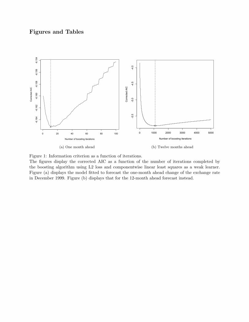
Figures and Tables

0 20 40 60 80 100

-6.164

-6.162

-6.160

-6.158

-6.156

-6.154

Number of boosting iterations

Cor

rect

ed A

IC

(a) One month ahead

0 1000 2000 3000 4000 5000-5.5

-5.0

-4.5

-4.0

Number of boosting iterations

Cor

rect

ed A

IC

(b) Twelve months ahead

Figure 1: Information criterion as a function of iterations.

The figures display the corrected AIC as a function of the number of iterations completed by

the boosting algorithm using L2 loss and componentwise linear least squares as a weak learner.

Figure (a) displays the model fitted to forecast the one-month ahead change of the exchange rate

in December 1999. Figure (b) displays that for the 12-month ahead forecast instead.

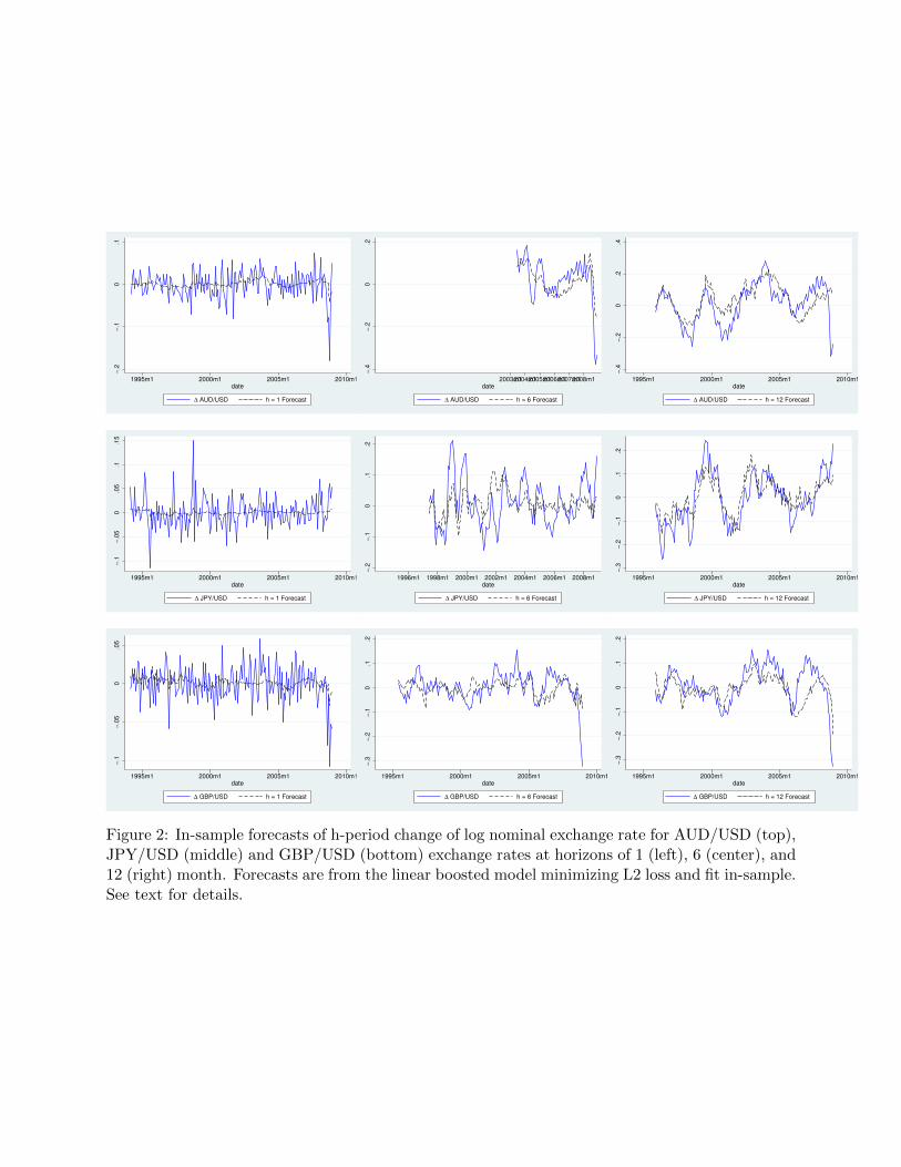
−.2

−.1

0.1

1995m1 2000m1 2005m1 2010m1

date

∆ AUD/USD h = 1 Forecast

−.4

−.2

0.2

2003m12004m12005m12006m12007m12008m1

date

∆ AUD/USD h = 6 Forecast

−.4

−.2

0.2

.4

1995m1 2000m1 2005m1 2010m1

date

∆ AUD/USD h = 12 Forecast

−.1

−.0

50

.05

.1.1

5

1995m1 2000m1 2005m1 2010m1

date

∆ JPY/USD h = 1 Forecast

−.2

−.1

0.1

.2

1996m1 1998m1 2000m1 2002m1 2004m1 2006m1 2008m1

date

∆ JPY/USD h = 6 Forecast

−.3

−.2

−.1

0.1

.2

1995m1 2000m1 2005m1 2010m1

date

∆ JPY/USD h = 12 Forecast

−.1

−.0

50

.05

1995m1 2000m1 2005m1 2010m1

date

∆ GBP/USD h = 1 Forecast

−.3

−.2

−.1

0.1

.2

1995m1 2000m1 2005m1 2010m1

date

∆ GBP/USD h = 6 Forecast

−.3

−.2

−.1

0.1

.2

1995m1 2000m1 2005m1 2010m1

date

∆ GBP/USD h = 12 Forecast

Figure 2: In-sample forecasts of h-period change of log nominal exchange rate for AUD/USD (top),

JPY/USD (middle) and GBP/USD (bottom) exchange rates at horizons of 1 (left), 6 (center), and

12 (right) month. Forecasts are from the linear boosted model minimizing L2 loss and fit in-sample.

See text for details.

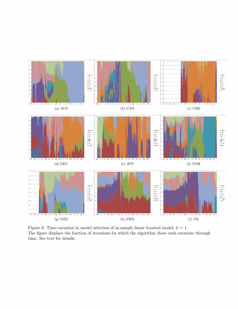
(a) AUS (b) CAN (c) CHE

(d) DEU (e) JPN (f) NOR

(g) NZD (h) SWE (i) UK

Figure 3: Time-variation in model selection of in-sample linear boosted model, h = 1.

The figure displays the fraction of iterations for which the algorithm chose each covariate through

time. See text for details.

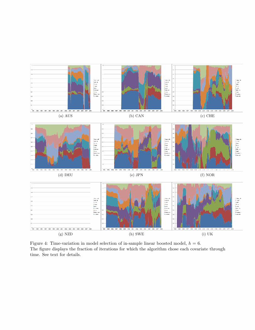
(a) AUS (b) CAN (c) CHE

(d) DEU (e) JPN (f) NOR

(g) NZD (h) SWE (i) UK

Figure 4: Time-variation in model selection of in-sample linear boosted model, h = 6.

The figure displays the fraction of iterations for which the algorithm chose each covariate through

time. See text for details.

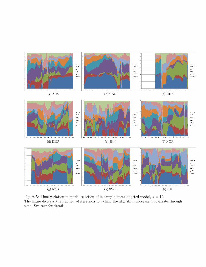
(a) AUS (b) CAN (c) CHE

(d) DEU (e) JPN (f) NOR

(g) NZD (h) SWE (i) UK

Figure 5: Time-variation in model selection of in-sample linear boosted model, h = 12.

The figure displays the fraction of iterations for which the algorithm chose each covariate through

time. See text for details.

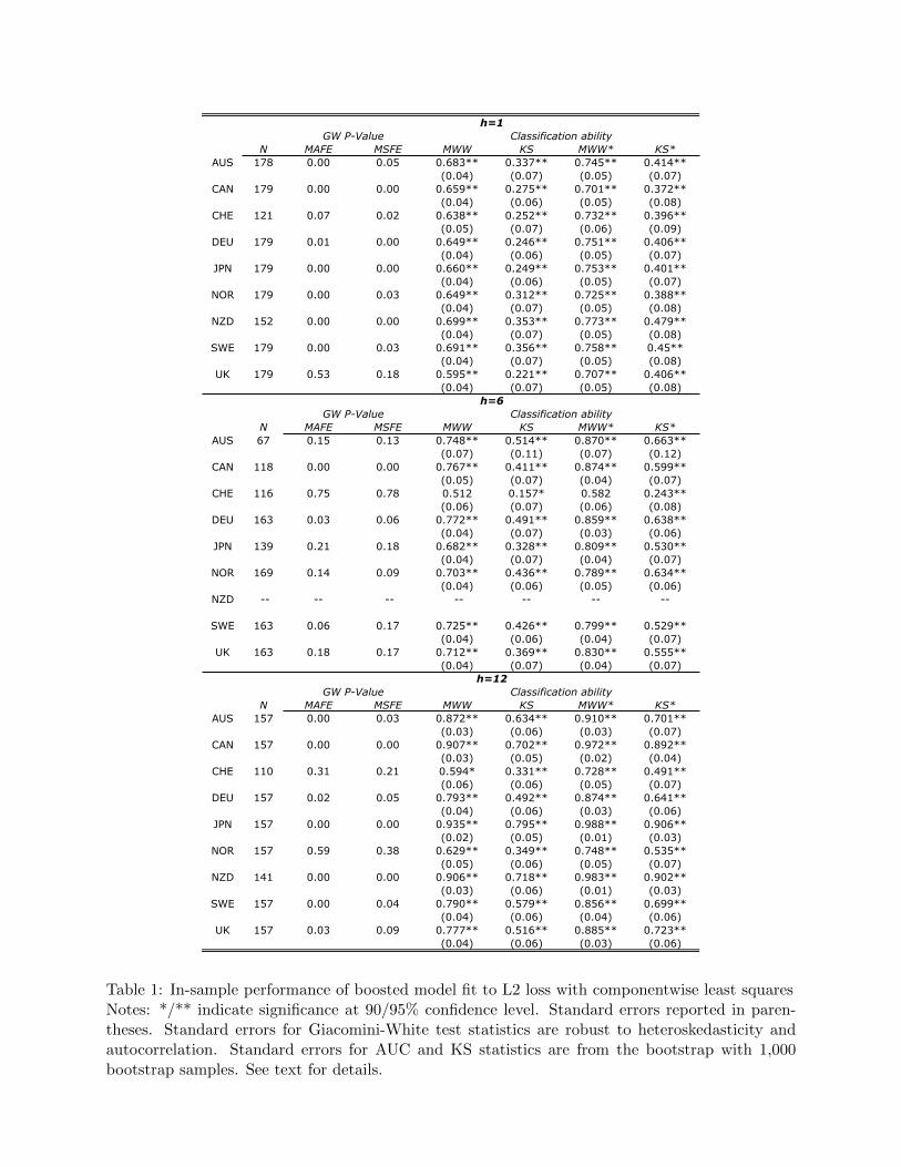
N MAFE MSFE MWW KS MWW* KS*AUS 178 0.00 0.05 0.683** 0.337** 0.745** 0.414**

(0.04) (0.07) (0.05) (0.07)CAN 179 0.00 0.00 0.659** 0.275** 0.701** 0.372**

(0.04) (0.06) (0.05) (0.08)CHE 121 0.07 0.02 0.638** 0.252** 0.732** 0.396**

(0.05) (0.07) (0.06) (0.09)DEU 179 0.01 0.00 0.649** 0.246** 0.751** 0.406**

(0.04) (0.06) (0.05) (0.07)JPN 179 0.00 0.00 0.660** 0.249** 0.753** 0.401**

(0.04) (0.06) (0.05) (0.07)NOR 179 0.00 0.03 0.649** 0.312** 0.725** 0.388**

(0.04) (0.07) (0.05) (0.08)NZD 152 0.00 0.00 0.699** 0.353** 0.773** 0.479**

(0.04) (0.07) (0.05) (0.08)SWE 179 0.00 0.03 0.691** 0.356** 0.758** 0.45**

(0.04) (0.07) (0.05) (0.08)UK 179 0.53 0.18 0.595** 0.221** 0.707** 0.406**

(0.04) (0.07) (0.05) (0.08)

N MAFE MSFE MWW KS MWW* KS*AUS 67 0.15 0.13 0.748** 0.514** 0.870** 0.663**

(0.07) (0.11) (0.07) (0.12)CAN 118 0.00 0.00 0.767** 0.411** 0.874** 0.599**

(0.05) (0.07) (0.04) (0.07)CHE 116 0.75 0.78 0.512 0.157* 0.582 0.243**

(0.06) (0.07) (0.06) (0.08)DEU 163 0.03 0.06 0.772** 0.491** 0.859** 0.638**

(0.04) (0.07) (0.03) (0.06)JPN 139 0.21 0.18 0.682** 0.328** 0.809** 0.530**

(0.04) (0.07) (0.04) (0.07)NOR 169 0.14 0.09 0.703** 0.436** 0.789** 0.634**

(0.04) (0.06) (0.05) (0.06)NZD -- -- -- -- -- -- --

SWE 163 0.06 0.17 0.725** 0.426** 0.799** 0.529**

(0.04) (0.06) (0.04) (0.07)UK 163 0.18 0.17 0.712** 0.369** 0.830** 0.555**

(0.04) (0.07) (0.04) (0.07)

N MAFE MSFE MWW KS MWW* KS*AUS 157 0.00 0.03 0.872** 0.634** 0.910** 0.701**

(0.03) (0.06) (0.03) (0.07)CAN 157 0.00 0.00 0.907** 0.702** 0.972** 0.892**

(0.03) (0.05) (0.02) (0.04)CHE 110 0.31 0.21 0.594* 0.331** 0.728** 0.491**

(0.06) (0.06) (0.05) (0.07)DEU 157 0.02 0.05 0.793** 0.492** 0.874** 0.641**

(0.04) (0.06) (0.03) (0.06)JPN 157 0.00 0.00 0.935** 0.795** 0.988** 0.906**

(0.02) (0.05) (0.01) (0.03)NOR 157 0.59 0.38 0.629** 0.349** 0.748** 0.535**

(0.05) (0.06) (0.05) (0.07)NZD 141 0.00 0.00 0.906** 0.718** 0.983** 0.902**

(0.03) (0.06) (0.01) (0.03)SWE 157 0.00 0.04 0.790** 0.579** 0.856** 0.699**

(0.04) (0.06) (0.04) (0.06)UK 157 0.03 0.09 0.777** 0.516** 0.885** 0.723**

(0.04) (0.06) (0.03) (0.06)

Classification ability

h=1

GW P-Value

GW P-Value Classification ability

GW P-Value Classification ability

h=6

h=12

Table 1: In-sample performance of boosted model fit to L2 loss with componentwise least squares

Notes: */** indicate significance at 90/95% confidence level. Standard errors reported in paren-

theses. Standard errors for Giacomini-White test statistics are robust to heteroskedasticity and

autocorrelation. Standard errors for AUC and KS statistics are from the bootstrap with 1,000

bootstrap samples. See text for details.

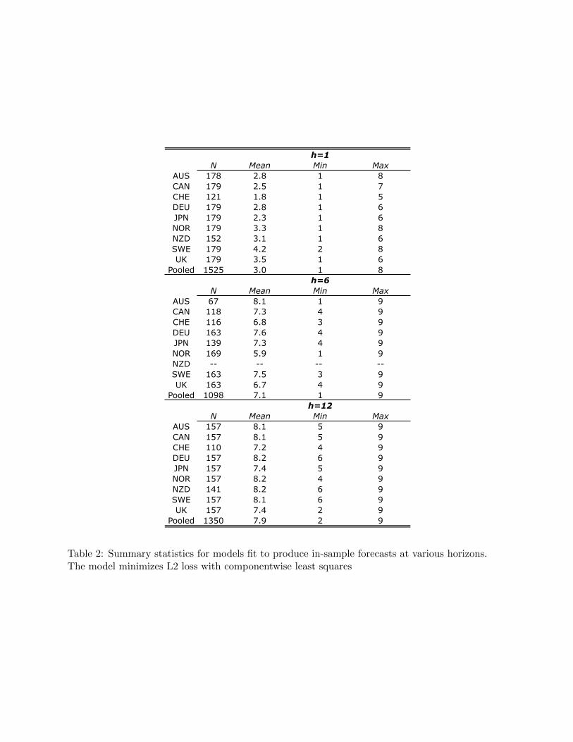
N Mean Min MaxAUS 178 2.8 1 8CAN 179 2.5 1 7CHE 121 1.8 1 5DEU 179 2.8 1 6JPN 179 2.3 1 6NOR 179 3.3 1 8NZD 152 3.1 1 6SWE 179 4.2 2 8UK 179 3.5 1 6

Pooled 1525 3.0 1 8

N Mean Min MaxAUS 67 8.1 1 9CAN 118 7.3 4 9CHE 116 6.8 3 9DEU 163 7.6 4 9JPN 139 7.3 4 9NOR 169 5.9 1 9NZD -- -- -- --SWE 163 7.5 3 9UK 163 6.7 4 9

Pooled 1098 7.1 1 9

N Mean Min MaxAUS 157 8.1 5 9CAN 157 8.1 5 9CHE 110 7.2 4 9DEU 157 8.2 6 9JPN 157 7.4 5 9NOR 157 8.2 4 9NZD 141 8.2 6 9SWE 157 8.1 6 9UK 157 7.4 2 9

Pooled 1350 7.9 2 9

h=1

h=6

h=12

Table 2: Summary statistics for models fit to produce in-sample forecasts at various horizons.

The model minimizes L2 loss with componentwise least squares

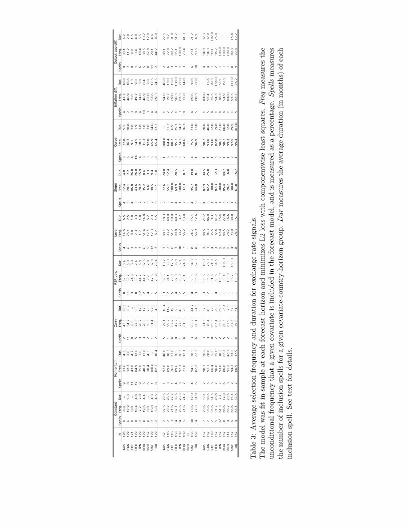
N

Spe

llsFr

eq.

!"#$

Spe

llsFr

eq.

!"#$

Spe

llsFr

eq.

!"#$

Spe

llsFr

eq.

!"#$

Spe

llsFr

eq.

!"#$

Spe

llsFr

eq.

!"#$

Spe

llsFr

eq.

!"#$

Spe

llsFr

eq.

!"#$

Spe

llsFr

eq.

!"#$

AU

S

178

00.

0--

923

.64.

32

43.3

38.5

839

.38.

44

14.6

6.5

412

.44.

88

77.0

5.5

442

.718

.89

33.1

6.2

CAN

17

96

17.9

5.3

812

.32.

811

54.7

8.9

1130

.75.

06

25.1

7.5

520

.17.

26

36.3

10.8

746

.910

.67

11.2

2.9

CH

E 12

10

0.8

--11

43.0

4.7

00.

8--

324

.08.

01

0.8

1.0

486

.826

.04

9.1

2.8

35.

81.

38

9.9

1.5

DEU

17

98

18.4

4.0

1284

.912

.05

22.3

8.0

835

.27.

43

7.3

3.3

343

.626

.014

14.5

1.9

849

.29.

01

3.4

4.0

JPN

17

92

2.2

2.0

935

.87.

03

20.7

12.3

1244

.75.

83

1.7

1.0

778

.215

.94

10.1

3.8

414

.03.

86

18.4

5.5

NO

R

179

819

.64.

45

40.2

13.8

328

.517

.02

44.7

37.5

651

.414

.87

35.2

8.6

831

.37.

010

46.9

8.4

538

.513

.2N

ZD

15

20

0.0

--6

18.4

4.3

230

.323

.04

9.9

2.8

517

.15.

23

6.6

3.3

392

.82.

03

67.8

7.0

867

.812

.9SW

E 17

97

16.8

4.3

110

0.0

--1

51.4

92.0

147

.582

.012

17.3

2.3

738

.59.

45

65.9

14.6

453

.617

.511

29.1

4.6

UK

179

25.

04.

58

82.7

18.4

25.

04.

55

70.9

25.4

26.

71.

53

1.7

1.0

965

.412

.74

69.3

24.5

244

.736

.0

AU

S

672

92.5

29.5

197

.048

.05

79.1

10.4

389

.618

.73

88.1

18.3

277

.624

.01

100.

0--

194

.046

.02

88.1

27.5

CAN

11

82

79.7

26.5

389

.818

.31

99.2

117.

02

94.1

35.0

293

.248

.05

55.1

12.4

664

.411

.72

79.7

13.0

672

.09.

7CH

E 11

63

71.6

27.7

176

.723

.04

67.2

19.5

579

.317

.66

51.7

10.0

110

0.0

--8

80.2

6.9

569

.015

.03

80.2

31.0

DEU

16

34

87.1

35.5

489

.636

.58

47.2

9.6

492

.036

.83

90.8

40.3

469

.928

.53

95.7

25.3

196

.313

8.0

395

.151

.7JP

N

139

475

.526

.33

92.1

26.3

177

.040

.02

95.0

6.0

1030

.23.

71

100.

0--

574

.114

.23

83.5

27.0

110

0.0

--N

OR

169

571

.624

.27

71.0

17.1

461

.526

.05

75.1

24.8

756

.213

.07

37.3

8.7

768

.616

.38

71.0

14.8

373

.441

.3N

ZD

0

----

----

----

----

----

----

----

----

----

----

----

----

----

--SW

E 16

310

73.6

12.0

494

.538

.53

82.2

44.7

485

.334

.38

74.2

15.1

495

.739

.04

75.5

23.0

489

.630

.06

79.1

21.2

UK

163

477

.331

.06

82.2

22.3

460

.124

.53

96.3

52.3

866

.912

.69

44.8

8.1

196

.911

.05

88.3

27.8

1059

.54.

9

AU

S

157

779

.65.

92

98.1

76.5

371

.337

.33

93.6

49.0

388

.521

.74

87.9

34.5

198

.728

.01

100.

0--

494

.937

.3CAN

15

72

93.6

58.5

591

.128

.63

76.4

40.0

296

.876

.01

94.3

86.0

582

.225

.81

93.0

46.0

592

.415

.64

94.3

32.0

CH

E 11

02

93.6

51.5

566

.45.

20

65.5

72.0

191

.821

.04

35.5

9.3

110

0.0

--1

93.6

12.0

475

.520

.31

99.1

107.

0D

EU

157

591

.728

.82

96.8

75.0

283

.429

.04

89.8

34.5

392

.441

.74

87.3

12.3

582

.819

.81

94.3

133.

02

96.2

75.0

JPN

15

712

64.3

7.1

293

.618

.52

52.9

39.5

110

0.0

--5

49.0

15.4

110

0.0

--2

98.1

21.0

478

.39.

31

100.

0--

NO

R

157

886

.617

.06

86.6

22.7

580

.323

.41

99.4

108.

05

88.5

27.8

385

.444

.71

98.7

66.0

494

.919

.31

100.

0--

NZD

14

14

83.7

29.5

391

.542

.72

87.9

7.5

110

0.0

--5

78.7

16.6

578

.716

.01

99.3

12.0

110

0.0

--1

100.

0--

SW

E 15

75

65.6

15.4

294

.373

.51

87.3

37.0

198

.713

0.0

493

.030

.01

100.

0--

297

.529

.51

97.5

111.

08

80.3

15.8

UK

157

483

.432

.57

80.9

17.9

479

.031

.01

100.

0--

878

.315

.16

61.8

15.7

199

.410

1.0

582

.225

.29

72.0

12.2

Infla

tion

diff.

Out

put

gap

diff.

Con

stan

tLe

vel

RER

dev

.Slo

peCur

veM

omen

tum

Car

ry

Table

3:Averageselectionfrequencyanddurationforexchangeratesignals.

Themodelwasfitin-sample

ateachforecasthorizonandminim

izesL2losswithcomponentw

iseleastsquares.Freqmeasuresthe

unconditionalfrequencythatagivencovariateisincludedin

theforecastmodel,andismeasuredasapercentage.Spellsmeasures

thenumberofinclusionspellsforagivencovariate-country-horizongroup.Durmeasurestheaverageduration(in

months)ofeach

inclusionspell.Seetextfordetails.

N MAFE MSFE AUC KS AUC* KS* AUS 177 0.601 0.716 0.575* 0.191** 0.588* 0.220**

(.04) (.07) (.05) (.08)CAN 178 0.607 0.249 0.536 0.134** 0.529 0.170*

(.05) (.07) (.06) (.09)CHE 120 0.122 0.325 0.469 0.081 0.481 0.149

(.06) (.08) (.07) (.10)DEU 178 0.496 0.345 0.519 0.120* 0.542 0.118*

(.04) (.06) (.05) (.07)JPN 178 0.334 0.491 0.527 0.092* 0.567 0.175**

(.04) (.05) (.06) (.08)NOR 178 0.913 0.499 0.527 0.098* 0.504 0.137**

(.04) (.05) (.06) (.05)NZD 151 0.211 0.916 0.609** 0.250** 0.596 0.266**

(.04) (.07) (.06) (.10)SWE 178 0.070 0.338 0.648** 0.290** 0.690** 0.343**

(.04) (.07) (.05) (.08)UK 178 0.017! 0.415 0.504 0.08 0.582 0.256**

(.04) (.05) (.06) (.09)

N MAFE MSFE AUC KS AUC* KS*AUS 66 0.791 0.454 0.675** 0.422** 0.789** 0.593**

(.08) (.12) (.09) (.13)CAN 117 0.126 0.220 0.659** 0.288** 0.694** 0.362**

(.05) (.07) (.09) (.11)CHE 115 0.233 0.214 0.442 0.058 0.467 0.114

(.06) (.07) (.07) (.08)DEU 162 0.281 0.656 0.703** 0.327** 0.773** 0.460**

(.04) (.07) (.04) (.07)JPN 138 0.989 0.994 0.605** 0.239** 0.730** 0.451**

(.05) (.07) (.06) (.07)NOR 168 0.838 0.979 0.652** 0.392** 0.707** 0.478**

(.05) (.07) (.06) (.08)NZD -- -- -- -- -- -- --

SWE 162 0.554 0.982 0.660** 0.331** 0.707** 0.418**(.05) (.07) (.06) (.09)

UK 162 0.983 0.716 0.646** 0.313** 0.748** 0.475**(.04) (.07) (.05) (.08)

N MAFE MSFE AUC KS AUC* KS* AUS 156 0.044 0.269 0.816** 0.567** 0.850** 0.618**

(.03) (.06) (.04) (.08)CAN 156 0.008 0.010 0.858** 0.608** 0.904** 0.733**

(.03) (.06) (.05) (.08)CHE 109 0.528 0.449 0.556 0.227** 0.677** 0.390**

(.06) (.07) (.06) (.07)DEU 156 0.113 0.186 0.755** 0.418** 0.846** 0.584**

(.04) (.07) (.03) (.06)JPN 156 0.000 0.000 0.910** 0.770** 0.977** 0.895**

(.03) (.05) (.01) (.03)NOR 156 0.677 0.763 0.554 0.251** 0.657** 0.360**

(.05) (.06) (.06) (.08)NZD 140 0.000 0.000 0.880** 0.639** 0.955** 0.778**

(.03) (.06) (.02) (.05)SWE 156 0.009 0.056 0.788** 0.563** 0.858** 0.694**

(.04) (.07) (.04) (.06)UK 156 0.203 0.382 0.747** 0.447** 0.838** 0.613**

(.04) (.06) (.04) (.06)

h=1

h=6

h=12

Table 4: Out-of-sample performance of boosted model fit to L2 loss with componentwise least

squares.

Notes: */** indicate significance at 90/95% confidence level. Standard errors reported in parenthe-

ses. Standard errors calculated for Giacomini-White test statistic are robust to heteroskedasticity

and autocorrelation. Standard errors for AUC and KS statistic are from the bootstrap with 1,000

bootstrap samples. See text for details.

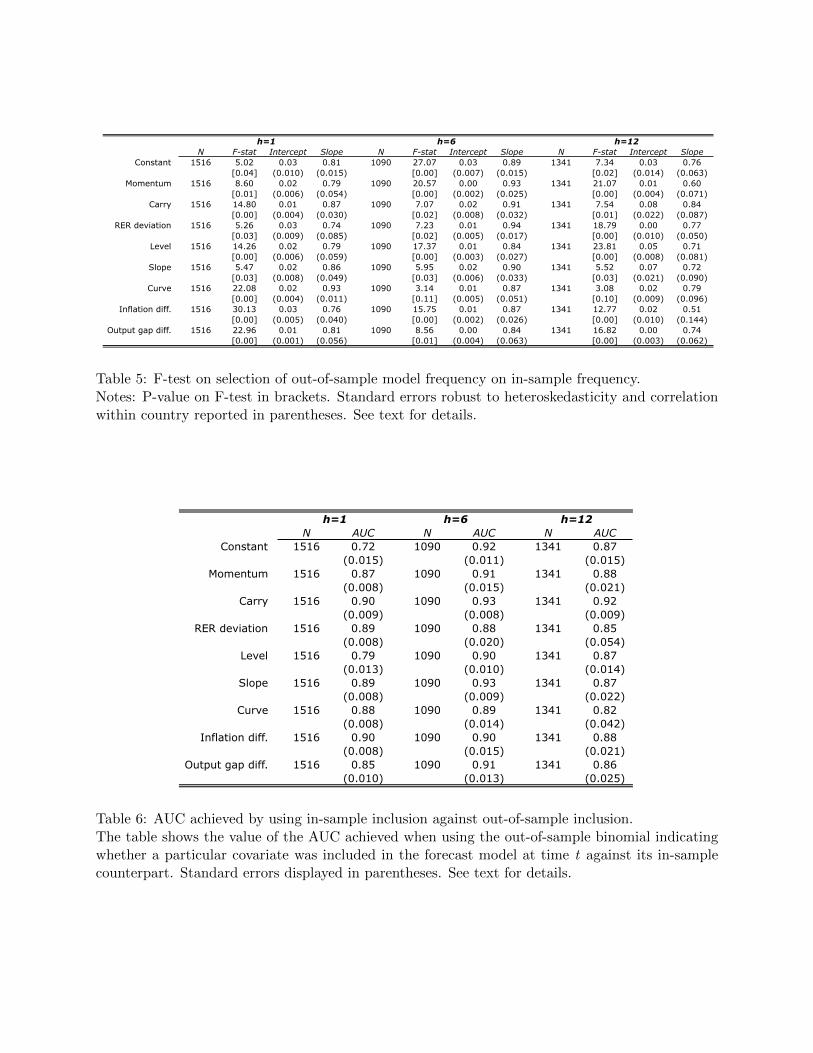
N F-stat Intercept Slope N F-stat Intercept Slope N F-stat Intercept SlopeConstant 1516 5.02 0.03 0.81 1090 27.07 0.03 0.89 1341 7.34 0.03 0.76

[0.04] (0.010) (0.015) [0.00] (0.007) (0.015) [0.02] (0.014) (0.063)Momentum 1516 8.60 0.02 0.79 1090 20.57 0.00 0.93 1341 21.07 0.01 0.60

[0.01] (0.006) (0.054) [0.00] (0.002) (0.025) [0.00] (0.004) (0.071)Carry 1516 14.80 0.01 0.87 1090 7.07 0.02 0.91 1341 7.54 0.08 0.84

[0.00] (0.004) (0.030) [0.02] (0.008) (0.032) [0.01] (0.022) (0.087)RER deviation 1516 5.26 0.03 0.74 1090 7.23 0.01 0.94 1341 18.79 0.00 0.77

[0.03] (0.009) (0.085) [0.02] (0.005) (0.017) [0.00] (0.010) (0.050)Level 1516 14.26 0.02 0.79 1090 17.37 0.01 0.84 1341 23.81 0.05 0.71

[0.00] (0.006) (0.059) [0.00] (0.003) (0.027) [0.00] (0.008) (0.081)Slope 1516 5.47 0.02 0.86 1090 5.95 0.02 0.90 1341 5.52 0.07 0.72

[0.03] (0.008) (0.049) [0.03] (0.006) (0.033) [0.03] (0.021) (0.090)Curve 1516 22.08 0.02 0.93 1090 3.14 0.01 0.87 1341 3.08 0.02 0.79

[0.00] (0.004) (0.011) [0.11] (0.005) (0.051) [0.10] (0.009) (0.096)Inflation diff. 1516 30.13 0.03 0.76 1090 15.75 0.01 0.87 1341 12.77 0.02 0.51

[0.00] (0.005) (0.040) [0.00] (0.002) (0.026) [0.00] (0.010) (0.144)Output gap diff. 1516 22.96 0.01 0.81 1090 8.56 0.00 0.84 1341 16.82 0.00 0.74

[0.00] (0.001) (0.056) [0.01] (0.004) (0.063) [0.00] (0.003) (0.062)

h=1 h=6 h=12

Table 5: F-test on selection of out-of-sample model frequency on in-sample frequency.

Notes: P-value on F-test in brackets. Standard errors robust to heteroskedasticity and correlation

within country reported in parentheses. See text for details.

N AUC N AUC N AUCConstant 1516 0.72 1090 0.92 1341 0.87

(0.015) (0.011) (0.015)Momentum 1516 0.87 1090 0.91 1341 0.88

(0.008) (0.015) (0.021)Carry 1516 0.90 1090 0.93 1341 0.92

(0.009) (0.008) (0.009)RER deviation 1516 0.89 1090 0.88 1341 0.85

(0.008) (0.020) (0.054)Level 1516 0.79 1090 0.90 1341 0.87

(0.013) (0.010) (0.014)Slope 1516 0.89 1090 0.93 1341 0.87

(0.008) (0.009) (0.022)Curve 1516 0.88 1090 0.89 1341 0.82

(0.008) (0.014) (0.042)Inflation diff. 1516 0.90 1090 0.90 1341 0.88

(0.008) (0.015) (0.021)Output gap diff. 1516 0.85 1090 0.91 1341 0.86

(0.010) (0.013) (0.025)

h=1 h=6 h=12

Table 6: AUC achieved by using in-sample inclusion against out-of-sample inclusion.

The table shows the value of the AUC achieved when using the out-of-sample binomial indicating

whether a particular covariate was included in the forecast model at time t against its in-sample

counterpart. Standard errors displayed in parentheses. See text for details.

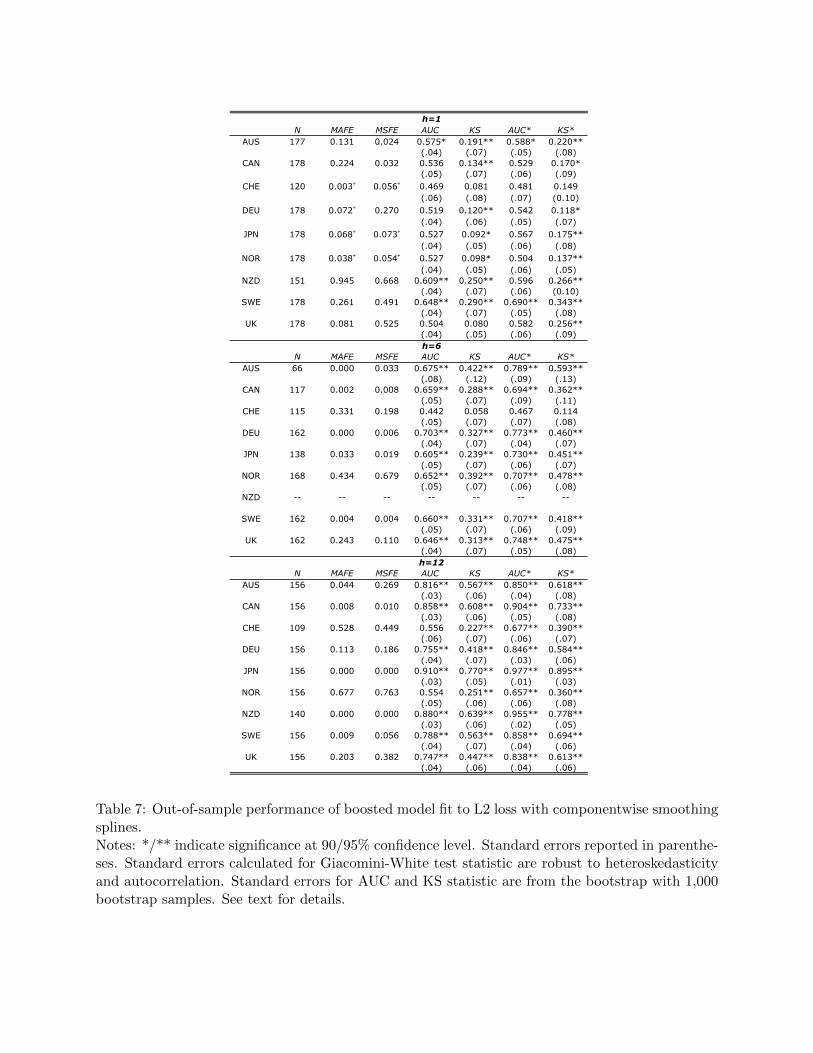
N MAFE MSFE AUC KS AUC* KS* AUS 177 0.131 0.024 0.575* 0.191** 0.588* 0.220**

(.04) (.07) (.05) (.08)CAN 178 0.224 0.032 0.536 0.134** 0.529 0.170*

(.05) (.07) (.06) (.09)CHE 120 0.003! 0.056! 0.469 0.081 0.481 0.149

(.06) (.08) (.07) (0.10)DEU 178 0.072! 0.270 0.519 0.120** 0.542 0.118*

(.04) (.06) (.05) (.07)JPN 178 0.068! 0.073! 0.527 0.092* 0.567 0.175**

(.04) (.05) (.06) (.08)NOR 178 0.038! 0.054! 0.527 0.098* 0.504 0.137**

(.04) (.05) (.06) (.05)NZD 151 0.945 0.668 0.609** 0.250** 0.596 0.266**

(.04) (.07) (.06) (0.10)SWE 178 0.261 0.491 0.648** 0.290** 0.690** 0.343**

(.04) (.07) (.05) (.08)UK 178 0.081 0.525 0.504 0.080 0.582 0.256**

(.04) (.05) (.06) (.09)

N MAFE MSFE AUC KS AUC* KS* AUS 66 0.000 0.033 0.675** 0.422** 0.789** 0.593**

(.08) (.12) (.09) (.13)CAN 117 0.002 0.008 0.659** 0.288** 0.694** 0.362**

(.05) (.07) (.09) (.11)CHE 115 0.331 0.198 0.442 0.058 0.467 0.114

(.05) (.07) (.07) (.08)DEU 162 0.000 0.006 0.703** 0.327** 0.773** 0.460**

(.04) (.07) (.04) (.07)JPN 138 0.033 0.019 0.605** 0.239** 0.730** 0.451**

(.05) (.07) (.06) (.07)NOR 168 0.434 0.679 0.652** 0.392** 0.707** 0.478**

(.05) (.07) (.06) (.08)NZD -- -- -- -- -- -- --

SWE 162 0.004 0.004 0.660** 0.331** 0.707** 0.418**(.05) (.07) (.06) (.09)

UK 162 0.243 0.110 0.646** 0.313** 0.748** 0.475**(.04) (.07) (.05) (.08)

N MAFE MSFE AUC KS AUC* KS* AUS 156 0.044 0.269 0.816** 0.567** 0.850** 0.618**

(.03) (.06) (.04) (.08)CAN 156 0.008 0.010 0.858** 0.608** 0.904** 0.733**

(.03) (.06) (.05) (.08)CHE 109 0.528 0.449 0.556 0.227** 0.677** 0.390**

(.06) (.07) (.06) (.07)DEU 156 0.113 0.186 0.755** 0.418** 0.846** 0.584**

(.04) (.07) (.03) (.06)JPN 156 0.000 0.000 0.910** 0.770** 0.977** 0.895**

(.03) (.05) (.01) (.03)NOR 156 0.677 0.763 0.554 0.251** 0.657** 0.360**

(.05) (.06) (.06) (.08)NZD 140 0.000 0.000 0.880** 0.639** 0.955** 0.778**

(.03) (.06) (.02) (.05)SWE 156 0.009 0.056 0.788** 0.563** 0.858** 0.694**

(.04) (.07) (.04) (.06)UK 156 0.203 0.382 0.747** 0.447** 0.838** 0.613**

(.04) (.06) (.04) (.06)

h=1

h=6

h=12

Table 7: Out-of-sample performance of boosted model fit to L2 loss with componentwise smoothing

splines.

Notes: */** indicate significance at 90/95% confidence level. Standard errors reported in parenthe-

ses. Standard errors calculated for Giacomini-White test statistic are robust to heteroskedasticity

and autocorrelation. Standard errors for AUC and KS statistic are from the bootstrap with 1,000

bootstrap samples. See text for details.

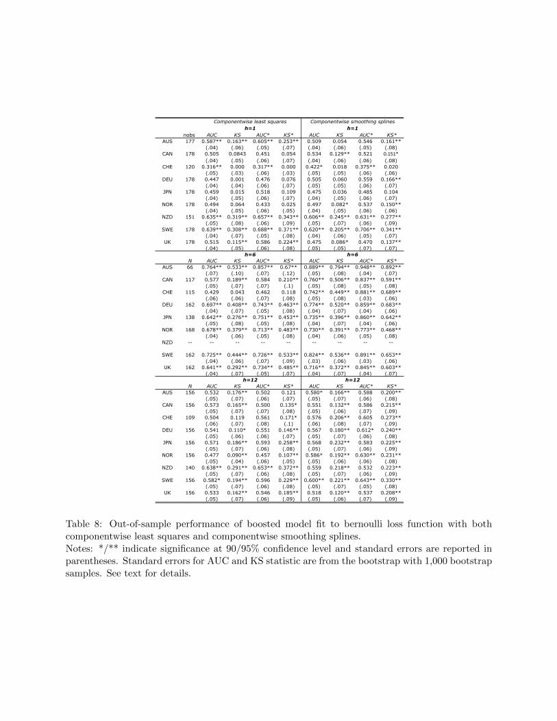
nobs AUC KS AUC* KS* AUC KS AUC* KS*AUS 177 0.587** 0.163** 0.605** 0.253** 0.509 0.054 0.546 0.161**

(.04) (.06) (.05) (.07) (.04) (.06) (.05) (.08)CAN 178 0.505 0.0843 0.451 0.054 0.534 0.129** 0.521 !"#$#%

(.04) (.05) (.06) (.07) (.04) (.06) (.06) (.08)CHE 120 0.316** 0.000 0.317** 0.000 0.422* 0.018 0.375** 0.020

(.05) (.03) (.06) (.03) (.05) (.05) (.06) (.06)DEU 178 0.447 0.001 0.476 0.076 0.505 0.060 0.559 0.166**

(.04) (.04) (.06) (.07) (.05) (.05) (.06) (.07)JPN 178 0.459 0.015 0.518 0.109 0.475 0.036 0.485 0.104

(.04) (.05) (.06) (.07) (.04) (.05) (.06) (.07)NOR 178 0.494 0.064 0.433 0.025 0.497 0.082* 0.537 0.150**

(.04) (.05) (.06) (.05) (.04) (.05) (.06) (.06)NZD 151 0.635** 0.319** 0.657** 0.343** 0.606** 0.245** 0.631** 0.277**

(.05) (.08) (.06) (.09) (.05) (.07) (.06) (.09)SWE 178 0.639** 0.308** 0.688** 0.371** 0.620** 0.205** 0.706** 0.341**

(.04) (.07) (.05) (.08) (.04) (.06) (.05) (.07)UK 178 0.515 0.115** 0.586 0.224** 0.475 0.086* 0.470 0.137**

(.04) (.05) (.06) (.08) (.05) (.05) (.07) (.07)

N AUC KS AUC* KS* AUC KS AUC* KS*AUS 66 0.764** 0.533** 0.857** 0.67** 0.889** 0.794** 0.948** 0.892**

(.07) (.10) (.07) (.12) (.05) (.08) (.04) (.07)CAN 117 0.577 0.189** 0.584 0.210** 0.760** 0.506** 0.837** 0.591**

(.05) (.07) (.07) (.1) (.05) (.08) (.05) (.08)CHE 115 0.429 0.043 0.462 0.118 0.742** 0.449** 0.881** 0.689**

(.06) (.06) (.07) (.08) (.05) (.08) (.03) (.06)DEU 162 0.697** 0.408** 0.743** 0.463** 0.774** 0.520** 0.859** 0.683**

(.04) (.07) (.05) (.08) (.04) (.07) (.04) (.06)JPN 138 0.642** 0.276** 0.751** 0.453** 0.735** 0.396** 0.860** 0.642**

(.05) (.08) (.05) (.08) (.04) (.07) (.04) (.06)NOR 168 0.678** 0.379** 0.713** 0.483** 0.730** 0.391** 0.773** 0.468**

(.04) (.06) (.05) (.08) (.04) (.06) (.05) (.08)NZD -- -- -- -- -- -- -- -- --

SWE 162 0.725** 0.444** 0.726** 0.533** 0.824** 0.536** 0.891** 0.653**(.04) (.06) (.07) (.09) (.03) (.06) (.03) (.06)

UK 162 0.641** 0.292** 0.734** 0.485** 0.716** 0.372** 0.845** 0.603**(.04) (.07) (.05) (.07) (.04) (.07) (.04) (.07)

N AUC KS AUC* KS* AUC KS AUC* KS*AUS 156 0.532 0.176** 0.502 0.121 0.580* 0.166** 0.588 0.200**

(.05) (.07) (.06) (.07) (.05) (.07) (.06) (.08)CAN 156 0.573 0.165** 0.500 0.135* 0.551 0.132** 0.586 0.215**

(.05) (.07) (.07) (.08) (.05) (.06) (.07) (.09)CHE 109 0.504 0.119 0.561 0.171* 0.576 0.206** 0.605 0.273**

(.06) (.07) (.08) (.1) (.06) (.08) (.07) (.09)DEU 156 0.541 0.110* 0.551 0.146** 0.567 0.180** 0.612* 0.240**

(.05) (.06) (.06) (.07) (.05) (.07) (.06) (.08)JPN 156 0.571 0.186** 0.593 0.258** 0.568 0.232** 0.583 0.225**

(.05) (.07) (.06) (.08) (.05) (.07) (.06) (.09)NOR 156 0.477 0.090** 0.457 0.107** 0.586* 0.192** 0.630** 0.231**

(.05) (.04) (.06) (.05) (.05) (.06) (.06) (.08)NZD 140 0.638** 0.291** 0.653** 0.372** 0.559 0.218** 0.532 0.223**

(.05) (.07) (.06) (.08) (.05) (.07) (.06) (.09)SWE 156 0.582* 0.194** 0.596 0.229** 0.600** 0.221** 0.643** 0.330**

(.05) (.07) (.06) (.08) (.05) (.07) (.05) (.08)UK 156 0.533 0.162** 0.546 0.185** 0.518 0.120** 0.537 0.208**

(.05) (.07) (.06) (.09) (.05) (.06) (.07) (.09)

h=12 h=12

Componentwise least squares Componentwise smoothing splinesh=1 h=1

h=6 h=6

Table 8: Out-of-sample performance of boosted model fit to bernoulli loss function with both

componentwise least squares and componentwise smoothing splines.

Notes: */** indicate significance at 90/95% confidence level and standard errors are reported in

parentheses. Standard errors for AUC and KS statistic are from the bootstrap with 1,000 bootstrap

samples. See text for details.

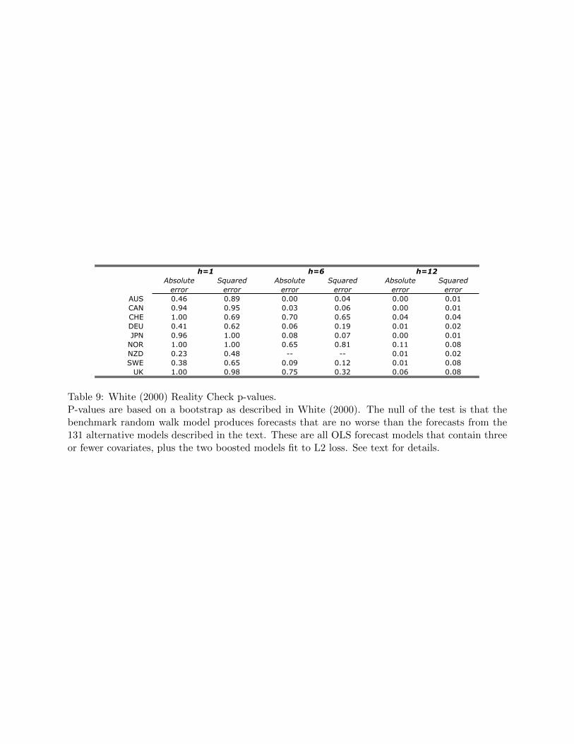
Absolute Squared Absolute Squared Absolute Squarederror error error error error error

AUS 0.46 0.89 0.00 0.04 0.00 0.01CAN 0.94 0.95 0.03 0.06 0.00 0.01CHE 1.00 0.69 0.70 0.65 0.04 0.04DEU 0.41 0.62 0.06 0.19 0.01 0.02JPN 0.96 1.00 0.08 0.07 0.00 0.01

NOR 1.00 1.00 0.65 0.81 0.11 0.08NZD 0.23 0.48 -- -- 0.01 0.02SWE 0.38 0.65 0.09 0.12 0.01 0.08

UK 1.00 0.98 0.75 0.32 0.06 0.08

h=1 h=6 h=12

Table 9: White (2000) Reality Check p-values.

P-values are based on a bootstrap as described in White (2000). The null of the test is that the

benchmark random walk model produces forecasts that are no worse than the forecasts from the

131 alternative models described in the text. These are all OLS forecast models that contain three

or fewer covariates, plus the two boosted models fit to L2 loss. See text for details.