forecasting for the generation of trading signals in financial markets

Forecasting for the Generation ofTrading Signals in Financial Markets

KIN LAM1* AND KING CHUNG LAM2

1Hong Kong Baptist University, Hong Kong2The University of Hong Kong, Hong Kong

ABSTRACT

In this paper we show that optimal trading results can be achieved if we canforecast a key summary statistic of future prices. Consider the followingoptimization problem. Let the return ri (over time i � 1, 2, . . . , n) for the ithday be given and the investor has to make investment decision di on the ithday with di � 1 representing a `long' position and di � 0 a `neutral'position. The investment return is given by r � Pn

i�1 ridi ÿ cPn�1

i�1 jdiÿdiÿ1j, where c is the transaction cost. The mathematical programmingproblem of choosing d1 , . . . , dn to maximize r under a given transaction costc is shown to have an analytic solution, which is a function of a keysummary statistic called the largest change before reversal. The largestchange before reversal is recommended to be used as an output in a neuralnetwork for the generation of trading signals. When neural networkforecasting is applied to a dataset of Hang Seng Index Futures Contracttraded in Hong Kong, it is shown that forecasting the largest change beforereversal outperforms the k-step-ahead forecast in achieving higher tradingpro®ts. Copyright # 2000 John Wiley & Sons, Ltd.

KEY WORDS ®nance; forecasting; trading rules; largest change beforereversal; neural network

`Buy low, sell high' is an investment dictum which is easier said than done. Trading decisions haveto be made without the knowledge of future prices and therefore it is impossible to determinewhether the current price is a low or a high. For a trading rule to be practicable, it has to satisfythe Markov property as de®ned in Neftci (1991), which is equivalent to saying that tradingdecisions can only utilize past but not future price information. For the pro®tability of sometechnical trading rules using past information only, see Taylor (1994) and Corrado and Lee(1992). However, even if we are allowed to make use of future information, it may still be a non-trivial problem to devise an optimal strategy, as we will explain below.

Consider an asset whose prices ¯uctuate from day to day and the closing price on the tth day(t � 0, 1, 2, . . . , n) is qt . Let pt � ln qt be the log-price and rt � pt ÿ ptÿ1 be the continuouslycompounded return on day t. An investment decision is a vector d � (d1 , d2 , . . . , dn), where

CCC 0277±6693/2000/010039±14$17.50 Received July 1997Copyright # 2000 John Wiley & Sons, Ltd. Accepted December 1998

Journal of Forecasting

J. Forecast. 19, 39±52 (2000)

* Correspondence to: Kin Lam, Department of Finance and Decision Sciences, School of Business, Hong Kong BaptistUniversity, 224 Waterloo Road, Kowloon, Hong Kong.

di � 0 or 1, meaning that the investor maintains a `neutral' or a `long' position respectively onday i. Here, we assume that the strategy of short-selling the asset is not available to the investor.This restriction can be lifted by allowing di � ÿ1, but we will carry out the discussion here usingthe simpli®ed version of restricting di to be 0 or 1. Assuming that the investor starts with a certainsum of money and is fully invested when a `long' position is taken, the investment returncorresponding to the decision d is given by r � Pn

i�1 ridi. Assuming that r1 , . . . , rn are known, rcan be maximized by choosing di � 1, if ri4 0 and di � 0, if ri4 0.

The optimization problem becomes non-trivial when transaction cost is taken into account.Whenever the investment decision di�1 is such that di 6� di�1, a transaction cost of 100c% isincurred. Assuming that the investor has a neutral position in the beginning and in the end,i.e. d0 � dn�1 � 0, the investment return is given by

r �Xni�1

ridi ÿ cXn�1i�1jdi ÿ diÿ1j

The mathematical programming problem (*) of maximizing r with given r1 , . . . , rn and d0 �dn�1 � 0 becomes non-trivial. The solution of (*) will be discussed in later sections of this paper.In the next section, we give a justi®cation of why (*) is of practical interest and why it hasimportant implications of forecasting for the generation of trading signals in a ®nancial market.

FORECASTING FOR THE GENERATION OF TRADING SIGNALS

At ®rst sight, the solution of (*) is of no practical interest because the optimal trading decision attime t depends on the values of rt�1 , rt�2 , . . . and is hence not Markov in the sense of Neftci(1991). However, the solution of (*) can give great insights as to which quantity is to be forecastedfor the generation of trading signals. When the market satis®es the weak-form market e�ciencyin the sense of Fama (1971), the e�orts of generating trading signals would be futile. However,according to Brock, Lakonishok and LeBaron (1992), the e�cient market hypothesis has comeunder serious siege in recent years. Serial correlation in returns over various investment horizonsare reported for individual stocks as well as for various portfolio of stocks; see, for example,Fama and French (1986), Poterba and Summers (1988), Jegadeesh (1990), and Cutler, Poterbaand Summers (1990). The correlations are statistically signi®cant and sometimes are of magni-tudes that could not be explained by non-synchronous trading or by the existence of marketfriction such as bid/ask spread. This provides evidence for the predictability of equity returnsfrom past returns. Utilizing the Dow Jones Index from 1897 to 1986, Brock, Lakonishok andLeBaron (1992) showed that returns obtained from some popular trading strategies are notconsistent with the random walk model and the GARCH families of models. Beja and Goldman(1980) argued that prices do not always adjust quickly to information shocks and markets can bein short-run disequilibrium. Grossman and Stiglitz (1980) attributed the slow adjustment processto the cost of acquiring and evaluating information and the need to adjust to new information.The pro®tability of technical trading systems on ®nancials was reported by Dale and Workman(1981), and Taylor and Tari (1989). Lukac and Brorsen (1990) carried out a comprehensive test offutures market disequilibrium. Twenty-three trading systems were tested in thirty futures marketsfor eleven years. All but two trading systems had signi®cant gross returns. For currencies futures,Taylor (1994) reported that currency futures could have been traded pro®tably from 1982 to 1990

Copyright # 2000 John Wiley & Sons, Ltd. J. Forecast. 19, 39±52 (2000)

40 K. Lam and K. C. Lam

using the channel rule. The average payo�, net of transaction costs, was both statistically andeconomically signi®cant. Recently, Bessembinder and Chan (1995) pointed out that some Asianmarkets may not be as informationally e�cient as their US or European counterparts. Theyfound that some simple technical analysis can be quite successful in the emerging markets ofMalaysia, Thailand and Taiwan. The `break-even' transaction cost for some technical tradingrules was found to be as high as 1.57%.

Recently, there has been considerable research in using neural networks to generate tradingsignals in order to pro®t from a possibly ine�cient market. Such applications can be found inRefenes et al. (1993), Moody and Utans (1992), Mehta (1994) and in the collected work of Trippiand Turbon (1992). Historical data forming what is called a training set are needed for thetraining of a neural network. In the training set, the whole price series is given, satisfying theassumption in (*) that r1 , . . . , rn are known. Typically, the neural network is trained to forecastthe k-step-ahead price and trading signals will be generated with the help of the forecasted prices.In the training set, the k-step-ahead price, pt�k , is known and the network is trained to give aforecast as pÃt�k . After training, trading signals can be generated by the following rule:

long if p̂t�k 4 ptshort if p̂t�k 5 pt

��1�

This approach has been widely used in the literature; see, for example, Mehta (1994), Bjorn(1994) and Hsu et al. (1993).

The use of a neural network to forecast with the purpose of generating trading signals raisestwo general but important questions: (1) Which quantity should be forecasted? and (2) How dowe make use of the forecasted quantity to construct trading signals? In the k-step-ahead forecast,it is not clear how k should be chosen and we are not sure whether strategy (1) is the best way togenerate trading signals. Instead of making a single-step-ahead forecast, one can make multi-period forecasts, which help in tracing the path of the prices in detail. However, we cannot be surehow many periods should be used and how these forecasts can be utilized to construct tradingsignals. In Kimoto and Asakawa (1990), the authors chose to forecast a summary statistic offuture prices, which re¯ect the future dynamics of the price changes. The quantity to beforecasted is the weighted sum of the future weekly returns of TOPIX on the Tokyo StockExchange. As the weighted sum captures more future information, this may enhance theperformance of the trading signals generated. However, there is no theoretical reason why onesummary statistic should be preferred over another. By deriving the solution to the optimizationproblem (*), it is discovered that its analytic solution depends on a summary statistic called the`largest change before reversal'. This summary statistic will be described in detail in the nextsection. Since the optimal solution is a function of this summary statistic, it is clear how it can beused to generate trading signals.

On the other hand, it is possible to generate trading signals directly, bypassing the forecastingstep. One can train the network to generate trading signals directly from the inputs. In otherwords, the output of the network is not a quantity to be forecasted, but is a trading signal. Someapplications using this type of output are Chauvin (1994), Binks and Allinson (1991), Bergersonand Wunsch (1991), Margarita (1991) and Zaremba (1990). What we need here is a set of targettrading signals for the training of the neural network. In most cases, these target trading signalsare expert generated, as in Bergerson and Wunsch (1991), or from price patterns recognized bytechnical chartists, or from a patterns library, as in Binks and Allinson (1991). However, if it pays


Generation of Trading Signals in Financial Markets 41

to train the computer to learn the technical analysts' timing for when to buy and sell, it may bebetter to train the computer to learn the optimal buy/sell times which should be known as far asthe training set is concerned. Thus, an analytic solution for (*) is useful and can be used as outputin the training set so as to train the network to trade in the future.

LARGEST CHANGE BEFORE REVERSAL

In this section we assume that prices p0 , p1 , . . . , pn are known. At the end of day t, we de®ne astatistic depending on pt�1 , . . . , pn which summarizes the price movements after day t. Thissummary statistic is called the largest change before reversal and is denoted by Ct . To give arigorous de®nition of Ct , we ®rst de®ne Tt , the time for ®rst reversal, as follows. Let pt be theclosing price at the end of day t. When pt�14 pt , Tt is de®ned as the ®rst day after (t � 1) in whichthe price reverses to a level below pt , i.e. pTt4 pt . Similarly, when pt�1 5 pt, Tt is de®ned as the®rst day after (t � 1) in which the price reverses to a level above pt , i.e. pTt5 pt . If the reversalnever happens, de®ne Tt � n. Mathematically,

Tt �minfT : � pt�1�� pt ÿ pt�4 0 t � 15T4 ng ^ n if pt�1 6� ptt � 1 if pt�1 � pt

�Here the minimum of an empty set is taken to be 1 and a ^ b denotes min (a,b). We now de®neCt as follows:

Ct �max

t�14 j4Tt

� pj ÿ pt� if pt�1 ÿ pt 4 0

0 if pt�1 ÿ pt � 0min

t�14 j4Tt

� pj ÿ pt� if pt�1 ÿ pt 5 0

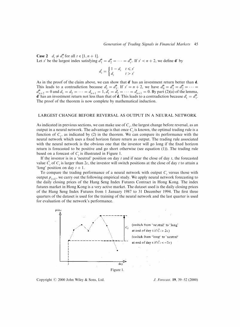
8>><>>:Ct is called the largest change before reversal. For a pictorial illustration of Ct , see Figure 1. If thereversal is from above pt to below pt , Ct is positive, meaning that the price ®rst goes up and risesto a maximum equal to pt � Ct before it drops below pt again. If the reversal is from below pt toabove pt , Ct is negative, meaning that the price ®rst drops to a minimum of pt � Ct before it risesto a level above pt .

The statistic Ct summarizes a lot of information about the price evolution after time t. Its signindicates whether the price is rising or not in the immediate future. Its magnitude indicateswhether it is worthwhile to buy or sell the asset. If the forecast is such that the price is rising butnot to a level enough to recover transaction costs, an investor should not switch from a neutralposition to a long position. Thus, it is natural to compare Ct with the transaction cost c. In thenext section, we will establish the theoretical importance of Ct by showing that it is closely relatedto the solution of (*).

OPTIMIZING TRADING PROFIT WITH FULL KNOWLEDGE OF PRICE CHANGES

In this section we state the theorem which gives an analytical solution for the optimizationproblem (*). The solution is given more generally in that the given value of d0 can either be 0 or 1.

Theorem Let r � Pni�1 ridi ÿ c

Pn�1i�1 jdi ÿ diÿ1j in which r0 , r1 , . . . , rn , d0 (�0 or 1) and dn�1

(�0) are given. Consider the problem (*) of maximizing r as a function of d1 , . . . , dn where di is



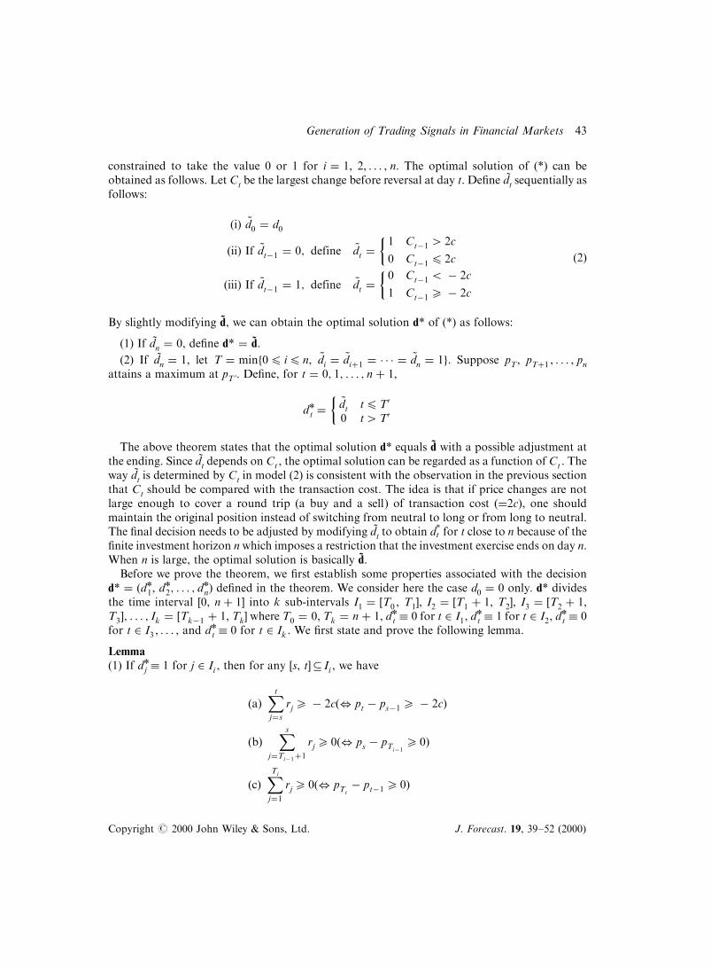
constrained to take the value 0 or 1 for i � 1, 2, . . . , n. The optimal solution of (*) can beobtained as follows. Let Ct be the largest change before reversal at day t. De®ne dÄt sequentially asfollows:

�i� ~d0 � d0

�ii� If ~dtÿ1 � 0; define ~dt �1 Ctÿ1 4 2c

0 Ctÿ1 4 2c

��iii� If ~dtÿ1 � 1; define ~dt �

0 Ctÿ1 5 ÿ 2c

1 Ctÿ1 5 ÿ 2c

� �2�

By slightly modifying dÄ , we can obtain the optimal solution d* of (*) as follows:

(1) If dÄn � 0, de®ne d* � dÄ .

(2) If dÄn � 1, let T � minf04 i4 n, ~di � ~di�1 � � � � � ~dn � 1g. Suppose pT, pT�1 , . . . , pnattains a maximum at pT 0. De®ne, for t � 0; 1; . . . ; n � 1,

d*t �~dt t4T0

0 t4T0

�The above theorem states that the optimal solution d* equals dÄ with a possible adjustment at

the ending. Since dÄt depends on Ct , the optimal solution can be regarded as a function of Ct . Theway dÄt is determined by Ct in model (2) is consistent with the observation in the previous sectionthat Ct should be compared with the transaction cost. The idea is that if price changes are notlarge enough to cover a round trip (a buy and a sell) of transaction cost (�2c), one shouldmaintain the original position instead of switching from neutral to long or from long to neutral.The ®nal decision needs to be adjusted by modifying dÄt to obtain d*t for t close to n because of the®nite investment horizon n which imposes a restriction that the investment exercise ends on day n.When n is large, the optimal solution is basically dÄ .

Before we prove the theorem, we ®rst establish some properties associated with the decisiond* � �d*1, d*2; . . . ; d*n) de®ned in the theorem. We consider here the case d0 � 0 only. d* dividesthe time interval [0, n � 1] into k sub-intervals I1 � [T0 , T1], I2 � �T1 � 1, T2], I3 � �T2 � 1,T3�; . . . ; Ik � �Tkÿ1 � 1, Tk] where T0 � 0, Tk � n � 1, d*t � 0 for t 2 I1, d*t � 1 for t 2 I2, d*t � 0for t 2 I3 , . . . , and d*t � 0 for t 2 Ik . We ®rst state and prove the following lemma.

Lemma(1) If d*j � 1 for j 2 Ii , then for any [s, t]� Ii , we have

�a�Xtj�s

rj 5 ÿ 2c�, pt ÿ psÿ1 5 ÿ 2c�

�b�Xs

j�Tiÿ1�1rj 5 0�, ps ÿ pTiÿ1

5 0�

�c�XTi

j�1rj 5 0�, pTt

ÿ ptÿ1 5 0�



(2) If d*j � 0 for j 2 Ii , then for any [s, t� � Ii , we have

�a�Xtj�s

rj 4 2c�, pt ÿ psÿ1 4 ÿ 2c�

�b�Xs

j�Tiÿ1�1rj 4 0�, ps ÿ pTiÿ1

4 0� for i 6� 1

�c�XTi

j�trj 5 0�, pTi

ÿ ptÿ1 4 0� for i 6� k

Proof of Lemma Instead of presenting the full proof, we give the proof for (1)(a) only. Suppose(1)(a) is false and we have pt ÿ psÿ1 5 ÿ 2c. It follows that among CSÿ1 , CS , . . . , Ctÿ1 , one ofthem, say Cw , has to be less than ÿ2c. This implies that d*w�1 is equal to 0, contradicting theassumption that d*j � 1 on [s, t]� Ii . The proofs of the other cases are similar.

Proof of Theorem Wewill prove the theorem by mathematical induction on n. Consider ®rst thecase n � 1. Obviously, C0 � p1 ÿ p0 and

d*1 �1 p1 ÿ p0 4 2c0 p1 ÿ p0 4 2c

�

It can be seen easily that d* is an optimal solution when n � 1.

Suppose the theorem has been established for n and we want to establish it for n � 1. Weassume that the theorem is not valid for n � 1 and let d be an optimal solution for n � 1 withinvestment return better than d* and d 6� d*. We will establish contradiction under two separatecases. Note that dn�2 � d*n�2 � 0.

Case 1 di � d*i for some i 2 �1; n � 1�.Let s(51) be the smallest index satisfying ds � d*s. If s � 1, contradiction arises because of theinduction assumption. If s4 1, let s0 be the largest index such that d*1 � d*2 � � � � � d*s0 . Lets* � min(s0, s) and de®ne d0 as follows:

d0i �

1 ÿ d*i i4 s*d*i i4 s*

�

Claim d0 has an investment return not less than that of d and hence not less than that of d*.

We will ®rst see how contradiction follows from the claim. This is because d01 � d*1 and by aninduction assumption, d0 cannot have an investment return better than that of d*.

To establish the claim, we consider one case in detail and omit the other cases, the proofs ofwhich are similar. The case we consider is s4 s0 � 1 and d01 � d02 � � � � � d*s0 � 0. For this case,d*s0�1 � 1, dS0�1 � 0, d1 � d2 � � � � � dS0 � 1. By de®nition of d0, d01 � d02 � � � � � d0S0 �1 � 1. Bypart (2)(c) of the lemma, it can be shown that the investment return of d0 is not less than that of d.



Case 2 dt 6� d*t for all t 2 �1; n � 1�.Let s0 be the largest index satisfying d*1 � d*2 � � � � � d*s0 . If s

05 n � 2, we de®ne d0 by

d0t �

1 ÿ dt t4 s0

dt t4 s0

�As in the proof of the claim above, we can show that d0 has an investment return better than d.This leads to a contradiction because d01 � d*1. If s0 � n � 2, we have d*0 � d*1 � d*2 � � � � �d*n�2 � 0 and d1 � d2 � � � � � dn�1 � 1, d01 � d02 � � � � � d0n�1 � 0. By part (2)(a) of the lemma,d0 has an investment return not less than that of d. This leads to a contradiction because d01 � d*1.The proof of the theorem is now complete by mathematical induction.

LARGEST CHANGE BEFORE REVERSAL AS OUTPUT IN A NEURAL NETWORK

As indicated in previous sections, we can make use of Ct , the largest change before reversal, as anoutput in a neural network. The advantage is that once Ct is known, the optimal trading rule is afunction of Ct , as indicated by (2) in the theorem. We can compare its performance with theneural network which uses a ®xed horizon future return as output. The trading rule associatedwith the neural network is the obvious one that the investor will go long if the ®xed horizonreturn is forecasted to be positive and go short otherwise (see equation (1)). The trading rulebased on a forecast of Ct is illustrated in Figure 1.

If the investor is in a `neutral' position on day t and if near the close of day t, the forecastedvalue CÃt of Ct is larger than 2c, the investor will switch positions at the close of day t to attain a`long' position on day t � 1.

To compare the trading performance of a neural network with output Ct versus those withoutput pt�k , we carry out the following empirical study. We apply neural network forecasting tothe daily closing prices of the Hang Seng Index Futures Contract in Hong Kong. The indexfutures market in Hong Kong is a very active market. The dataset used is the daily closing pricesof the Hang Seng Index Futures from 1 January 1987 to 31 December 1994. The ®rst threequarters of the dataset is used for the training of the neural network and the last quarter is usedfor evaluation of the network's performance.

Figure 1.



The neural network used is a multi-layer perceptron network with one hidden layer having ®veunits, a hyperbolic tangent transfer function, a sum of square error function and regulationtraining. Here, we only use a very simple network, the multi-layer perceptron network. Thereason is that in Chen et al. (1995) this simple network is shown to be a universal approximatorand can approximate any arbitrary function. We use the hyperbolic tangent transfer functionbecause it can incorporate both positive and negative outputs. Also, it is found that a networkwith the hyperbolic tangent transfer function can be trained faster than one with a sigmoidaltransfer function. The reason for using regulation training is that it is found to be very e�ective onthe short and noisy dataset by Weigend et al. (1992). Our dataset is short and noisy so theregulation training is very suitable.

For inputs to the neural network, we use the historical one-, two-, three-, ten-, twenty- andthirty-day returns, i.e. ln pt ÿ ln ptÿi with i � 1, 2, 3, 10, 20, and 30. We will use these inputs toforecast (1) Ct , the largest change before reversal and (2) ln pt�k ÿ ln pt, the future return with a®xed forecasting horizon of k � 5, 10, 20, and 30 days.

To compare the trading performance of (1) and (2), we rely on two performance measures, thepro®t in index points and the investment return. When the networks are trained to generate buy/sell signals for the last quarter of the data period, two trading performance measures will becomputed as follows. (1) We assume the investor to buy one contract on the ®rst recommendedbuy signal, cover up on the next `sell' signal, and buy another contract on the next `buy' signal,etc. Here, no reinvestment of pro®t is assumed. Let the m buy/sell signals occur at days withclosing indices x1 , x2 , . . . , xm , the pro®t in index points are, after taking transaction costs intoconsideration, calculated by

�x2 ÿ x1� � �x4 ÿ x3� � � � � � �xm ÿ xmÿ1� ÿ c�x1 � � � � � xm� if m is even�x2 ÿ x1� � �x4 ÿ x3� � � � � � �xmÿ1 ÿ xmÿ2� ÿ c�x1 � � � � � xmÿ1� if m is odd

�(2) To calculate the second performance measure called the investment return, note that themargin system in a futures market may a�ect the way how investment return can be computed.Here we follow Lukac, Br

.orsen and Irwin (1988) and assume no margining, i.e. the invested

capital is the full amount for a contract and is not just the initial margin. Thus, in the ®rstoccurrence of a `buy' signal, the investor goes long in one futures contract by putting up anamount V which is the worth of the contract. Assume that the `buy' signal occurs when the indexis x1 . If a `sell' signal then occurs at index value x2 , the futures contract is sold. The capital whichremains, assuming a round-trip transaction cost of 100(2c)%, is V�ln xn ÿ ln x1 ÿ 2c�. Thisamount of money is then fully invested in buying (ln x2 ÿ ln x1 ÿ 2c) futures contract on the next`buy' signal, without relying on the margining system. The accounting continues in this manneruntil the investor is left with an amount equal to Vf at the end. The investment return is thencalculated by ln Vfÿ ln V. In this paper, a round-trip transaction cost of 0.2% for a futurescontract is assumed.

In Table I, both performance measures are reported in the training period as well as in thetesting period (see rows 1 and 3 in Table I). Since the training of the network involves a randomstart in the beginning, both performance measures will depend on the random start. Ten randomstarts are alternative and the average performance measures as well as their standard deviations(over 10 trials) are reported (see rows 2 and 4 in Table I).

It can easily be seen from Table I that for most cases using Ct as output gives rise to a morepro®table trading strategy than that using ®xed-period return as output. The only exception is



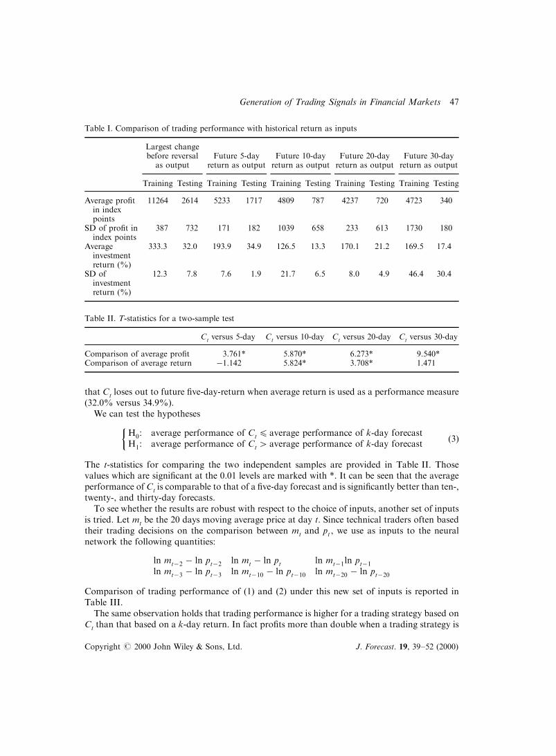
that Ct loses out to future ®ve-day-return when average return is used as a performance measure(32.0% versus 34.9%).

We can test the hypotheses

H0: average performance of Ct 4 average performance of k-day forecastH1: average performance of Ct 4 average performance of k-day forecast

��3�

The t-statistics for comparing the two independent samples are provided in Table II. Thosevalues which are signi®cant at the 0.01 levels are marked with *. It can be seen that the averageperformance of Ct is comparable to that of a ®ve-day forecast and is signi®cantly better than ten-,twenty-, and thirty-day forecasts.

To see whether the results are robust with respect to the choice of inputs, another set of inputsis tried. Let mt be the 20 days moving average price at day t. Since technical traders often basedtheir trading decisions on the comparison between mt and pt , we use as inputs to the neuralnetwork the following quantities:

ln mtÿ2 ÿ ln ptÿ2 ln mt ÿ ln pt ln mtÿ1ln ptÿ1ln mtÿ3 ÿ ln ptÿ3 ln mtÿ10 ÿ ln ptÿ10 ln mtÿ20 ÿ ln ptÿ20

Comparison of trading performance of (1) and (2) under this new set of inputs is reported inTable III.

The same observation holds that trading performance is higher for a trading strategy based onCt than that based on a k-day return. In fact pro®ts more than double when a trading strategy is

Table I. Comparison of trading performance with historical return as inputs

Largest changebefore reversal

as outputFuture 5-day

return as outputFuture 10-dayreturn as output

Future 20-dayreturn as output


Training Testing Training Testing Training Testing Training Testing Training Testing

Average pro®tin indexpoints

11264 2614 5233 1717 4809 787 4237 720 4723 340

SD of pro®t inindex points

387 732 171 182 1039 658 233 613 1730 180

Averageinvestmentreturn (%)

333.3 32.0 193.9 34.9 126.5 13.3 170.1 21.2 169.5 17.4

SD ofinvestmentreturn (%)

12.3 7.8 7.6 1.9 21.7 6.5 8.0 4.9 46.4 30.4

Table II. T-statistics for a two-sample test

Ct versus 5-day Ct versus 10-day Ct versus 20-day Ct versus 30-day

Comparison of average pro®t 3.761* 5.870* 6.273* 9.540*Comparison of average return ÿ1.142 5.824* 3.708* 1.471



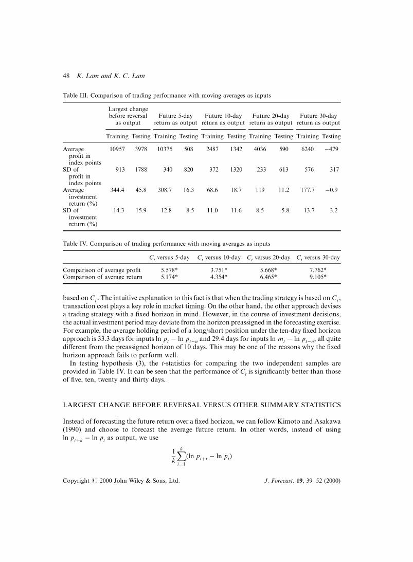
based on Ct . The intuitive explanation to this fact is that when the trading strategy is based on Ct ,transaction cost plays a key role in market timing. On the other hand, the other approach devisesa trading strategy with a ®xed horizon in mind. However, in the course of investment decisions,the actual investment period may deviate from the horizon preassigned in the forecasting exercise.For example, the average holding period of a long/short position under the ten-day ®xed horizonapproach is 33.3 days for inputs ln pt ÿ ln ptÿn and 29.4 days for inputs ln mt ÿ ln ptÿn, all quitedi�erent from the preassigned horizon of 10 days. This may be one of the reasons why the ®xedhorizon approach fails to perform well.

In testing hypothesis (3), the t-statistics for comparing the two independent samples areprovided in Table IV. It can be seen that the performance of Ct is signi®cantly better than thoseof ®ve, ten, twenty and thirty days.

LARGEST CHANGE BEFORE REVERSAL VERSUS OTHER SUMMARY STATISTICS

Instead of forecasting the future return over a ®xed horizon, we can follow Kimoto and Asakawa(1990) and choose to forecast the average future return. In other words, instead of usingln pt�k ÿ ln pt as output, we use

1

k

Xki�1�ln pt�i ÿ ln pt�

Table III. Comparison of trading performance with moving averages as inputs

Largest changebefore reversal

as outputFuture 5-day

return as outputFuture 10-dayreturn as output



Training Testing Training Testing Training Testing Training Testing Training Testing

Averagepro®t inindex points

10957 3978 10375 508 2487 1342 4036 590 6240 ÿ479

SD ofpro®t inindex points

913 1788 340 820 372 1320 233 613 576 317

Averageinvestmentreturn (%)

344.4 45.8 308.7 16.3 68.6 18.7 119 11.2 177.7 ÿ0.9

SD ofinvestmentreturn (%)

14.3 15.9 12.8 8.5 11.0 11.6 8.5 5.8 13.7 3.2

Table IV. Comparison of trading performance with moving averages as inputs

Ct versus 5-day Ct versus 10-day Ct versus 20-day Ct versus 30-day

Comparison of average pro®t 5.578* 3.751* 5.668* 7.762*Comparison of average return 5.174* 4.354* 6.465* 9.105*



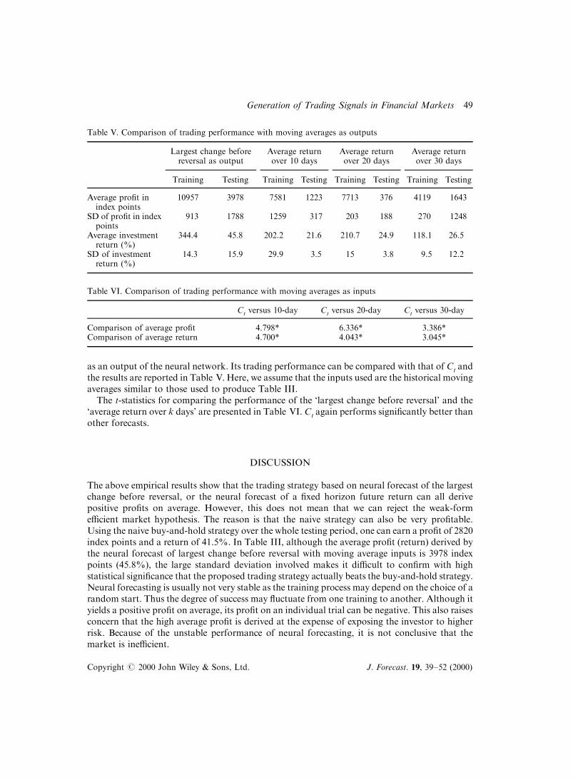
as an output of the neural network. Its trading performance can be compared with that of Ct andthe results are reported in Table V. Here, we assume that the inputs used are the historical movingaverages similar to those used to produce Table III.

The t-statistics for comparing the performance of the `largest change before reversal' and the`average return over k days' are presented in Table VI. Ct again performs signi®cantly better thanother forecasts.

DISCUSSION

The above empirical results show that the trading strategy based on neural forecast of the largestchange before reversal, or the neural forecast of a ®xed horizon future return can all derivepositive pro®ts on average. However, this does not mean that we can reject the weak-forme�cient market hypothesis. The reason is that the naive strategy can also be very pro®table.Using the naive buy-and-hold strategy over the whole testing period, one can earn a pro®t of 2820index points and a return of 41.5%. In Table III, although the average pro®t (return) derived bythe neural forecast of largest change before reversal with moving average inputs is 3978 indexpoints (45.8%), the large standard deviation involved makes it di�cult to con®rm with highstatistical signi®cance that the proposed trading strategy actually beats the buy-and-hold strategy.Neural forecasting is usually not very stable as the training process may depend on the choice of arandom start. Thus the degree of success may ¯uctuate from one training to another. Although ityields a positive pro®t on average, its pro®t on an individual trial can be negative. This also raisesconcern that the high average pro®t is derived at the expense of exposing the investor to higherrisk. Because of the unstable performance of neural forecasting, it is not conclusive that themarket is ine�cient.

Table V. Comparison of trading performance with moving averages as outputs

Largest change beforereversal as output

Average returnover 10 days



Training Testing Training Testing Training Testing Training Testing

Average pro®t inindex points

10957 3978 7581 1223 7713 376 4119 1643

SD of pro®t in indexpoints

913 1788 1259 317 203 188 270 1248

Average investmentreturn (%)

344.4 45.8 202.2 21.6 210.7 24.9 118.1 26.5

SD of investmentreturn (%)

14.3 15.9 29.9 3.5 15 3.8 9.5 12.2

Table VI. Comparison of trading performance with moving averages as inputs

Ct versus 10-day Ct versus 20-day Ct versus 30-day

Comparison of average pro®t 4.798* 6.336* 3.386*Comparison of average return 4.700* 4.043* 3.045*



Although we may not be able to reject the weak-form market e�ciency, the empirical ®ndingsin this paper show that the theoretical result derived in the theorem can be used to devise asuccessful trading rule which compares favourably with those based on ®xed±horizon forecasts.We should note here that although we forecast the largest change before reversal using a neuralnetwork, the same approach can be used together with other forecasting techniques. To forecastthe `largest change before reversal' has the advantage that it advises the investor to trade onlywhen the pro®t from doing so exceeds the cost, as pointed out by a referee of this paper. Thisconcept is of course an obvious one. However, it has not been practised by technical analysts informulating their trading rule. If a ®nancial analyst only forecasts the price ten days from now,there is no way to ®nd out whether the potential pro®t exceeds the cost in days other than thegiven time horizon. The empirical work carried out in this paper demonstrates that this intuitiveidea is implementable and it can strengthen the applicability of any potential technique in®nancial forecasting.

SUMMARY AND CONCLUSION

In this paper we show that optimal trading results can be achieved if we can forecast a keysummary statistic of future prices. The key summary statistic Ct , called the largest change beforereversal, is de®ned. Assuming future prices are completely known, the problem of constructingan optimal investment decision in the presence of a transaction cost c is formulated as amathematical programming problem. It is shown that the optimal solution for this programmingproblem is essentially a function of Ct . Thus the statistic Ct acts in some sense as a su�cientstatistic for an optimal trading strategy with transaction cost. Hence it is natural to focusattention on the forecast of Ct if the purpose of forecasting is to obtain a good trading rule.Empirical results also support the use of Ct as output in a neural network when it is applied to the®nancial market for the generation of trading signals.

REFERENCES

Beja, A. and Goldman, M. B. Òn the dynamic behavior of prices in disequilibrium', Journal of Finance, 34(1980), 235±47.

Bergerson, K. and Wunsch, D. C. II. À commodity trading model based on a neural network±expertsystem hybrid', IJCNN91, 1 (1991), 289±93.

Bessembinder, H. and Chan, K. `The pro®tability of technical trading rules in the Asian stock markets',Paci®c Basic Finance Journal, 3 (1995), 257±84.

Binks, D. L. and Allinson, N. M. `Financial data recognition and prediction using neural networks',Arti®cial Neural Networks, 1 (1991), 1709±12.

Bjorn, V. Òptimal multiresolution decomposition of ®nancial time series', in Refenes, A. N. (ed.), NeuralNetworks in the Capital Markets, Chichester: Wiley, 1994.

Brock, W., Lakonishok, J. and LeBaron, B. `Simple technical tracing rules and the stochastic properties ofstock returns', Journal of Finance, 5 (1992), 1731±65.

Chauvin, Y. `Trading Decision Learning: From Theory to Personal Traders', in Refenes, A. N. (ed.),Neural Networks in the Capital Markets, Chichester, U.S.A: John Wiley, 1994.

Chen, T. P., Chen, H. and Liu, R. W. Àpproximation capability in C(R) by multilayer feedforwardnetworks and related problems', in Refenes, A. N. (ed.), IEEE Transactions on Neural Networks, 6Chichester: Wiley, 1995, 25±30.



Corrado, C. J. and Lee, S. H. `Filter rule tests of economic signi®cance of serial dependencies in daily stockreturn', Journal of Financial Research, 15 (1992), 369±87.

Cutler, D. M., Poterba, J. M. and Summers, L. H. `Speculative dynamics', Review of Economic Studies, 58(1991), 529±46.

Dale, C. and Workman, R. `Patterns of price movement in Treasury bill futures', Journal of Economics andBusiness, 33 (1981), 81±7.

Fama, E. F. È�cient capital markets: a review of theory and empirical work', Journal of Finance, 25(1970), 383±417.

Fama, E. F. and French, K. R. `Permanent and temporary components of stock prices', Journal of PoliticalEconomy, 98 (1986), 246±74.

Grossman, S. J. and Stiglitz, J. E. Òn the impossibility and informationally e�cient markets', AmericanEconomic Review, 70 (1980), 393±408.

Hsu, W., Hsu, L. S. and Tenorio, M. F. `Parameter signi®cance estimation and ®nancial prediction', NeuralComputing and Application, 1 (1993), 280±6.

Jegadeesh, N. Èvidence of predictable behavior of securities returns', Journal of Finance, 45 (1990),881±98.

Kimoto, T. and Asakawa, K. `Stock market prediction system with modular neural networks', ProcIJCNN, San Diego, CA: 1, 1990, 1±6.

Lukac, L. P. and Brorsen, B. W. À comprehensive test of futures market disequilibrium', Journal ofFinance, 25 (1990), 593±622.

Lukac, L. P., Brorsen, B. W. and Irwin, S. H. À comparison of twelve technical trading systems withmarket e�ciency implications', Station Bulletin (1988), No. 495, Department of Agricultural Economics,Purdue University.

Margarita, S. `Neural network, genetic algorithms and stock trading', Arti®cial Neural Networks, 1 (1991),1763±6.

Mehta, M. `Trading in foreign exchange markets using Kalman ®lter and neural network', in Refenes, A. N.(ed.), Neural Networks in the Capital Markets, Chichester: Wiley, 1994.

Moody, J. and Utans, J. `Principled architecture selection for neural networks: application to corporatebond rating prediction', Advances in Neural Information Processing Systems, 4 (1992), 683±90.

Neftci, N. `Naive trading rules in ®nancial markets and Wiener±Kolmogorov prediction theory: a study of``technical analysis'' ', Journal of Business, 64 (1991), 549±71.

Poterba, J. L. and Summers, L. `Mean reversion in stock prices: evidence and implications', Journal ofFinancial Economics, 22 (1988), 27±59.

Refenes, A. N., Azema-Barac, M., Chan, L. and Karoussos, S. A. `Currency exchange rate prediction andneural network design strategies', Neural Computing and Applications, 1 (1993), 46±58.

Taylor, S. J. `Trading futures using a channel rule: a study of the predictive power of technical analysis withcurrency examples', The Journal of Futures Market, 14 No. 2 (1994), 215±35.

Taylor, S. J. and Tari, A. `Further evidence against the e�ciency of futures markets', in Guimaraes,R. M. C., Kingsman, B. G. and Taylor, S. J. (eds), A Reappraisal of the E�ciency of Financial Markets,New York: Springer-Verlag, 1989.

Trippi, R. and Turban, E. Neural Network Applications in Investment and Financial Services, New York:Probus Publishing, 1992.

Weigend, A. S., Huberman, B. A. and Rumelhart, D. E. `Predicting sunspots and exchange rates withconnectionist networks', Nonlinear Modeling and Forecasting, SFI Studies in the Sciences of Complexity,7 (1992), 395±432.

Zapranis, A. D. and Refenes, A. N. `Neural networks in tactical asset allocation: towards a methodologyfor hypothesis testing and con®dence intervals', Proceedings of Neural Networks in the Capital Markets,1994.

Zaremba, T. `Case Study III: Technology in search of a buck', Neural Network PC Tools, (1990), 251±83.



Authors' biographies:K. Lam obtained a PhD in Mathematics from the University of Wisconsin in 1972 and worked as a lecturer,senior lecturer and reader in the Department of Statistics in the University of Hong Kong. He took up thechair professorship in the Department of Finance and Decisions Sciences of the Hong Kong BaptistUniversity in January 1995 and has headed the department since then.

Charles K. C. Lam is studying for an MPhil degree and was a studentship holder in the Department ofStatistics in the University of Hong Kong from September 1994 to August 1996. He joined the Dao HengBank in Hong Kong where he has worked as an investment advisor since September 1996.

Authors' addresses:K. Lam, Department of Finance and Decision Sciences, School of Business, Hong Kong Baptist University,224 Waterloo Road, Kowloon, Hong Kong.

Charles K. C. Lam, Department of Statistics, The University of Hong Kong.



forecasting for the generation of trading signals in financial markets

Documents