Forecasting in STATA: Tools and Tricks

Introduction This manual is intended to be a reference guide for time-series forecasting in STATA. Working with Datasets If you have an existing STATA dataset, it is a file with the extension “.dta”. If you double-click on the file, it will typically open a STATA window and load the datafile into memory. If a STATA window is already active, and the data file is in the current working directory, you can load the file realgdp.dta by typing . use realgdp This only works if there is currently no data in memory. To erase the current data, you can first use the command . clear all Or, to simultaneously clear current data and load the new file, just type . use realgdp, clear If you want to save the file, type . save filename Where filename is the name you want to use. Stata will add a “.dta” extension. The save command only works if there is no file with that name. If you want to replace an existing file, you can use . save filename, replace Interactive Commands and Do Files Stata commands can be executed either one-at-a-time from the command line, or in batch as a do file. A do file is a text file, with a name such as “problemset1.do” where each line in the file is a single STATA command Execution from the command line is convenient for experimentation and learning about the language. Execution using a do file, however, is highly advisable for serious work, and for documenting your work. It is easier to execute a set of similar commands, as well, as you can easier use cut-and-paste in a text editor. By running your commands via a batch text file, you also have a record of your work, which can often be a great resource for your next project (e.g. next problem set). It is often smart for a do file to start the calculations from scratch. Start with clear and then load from a database such as FRED (documented below), or load a stata file using “use realgdp, clear”. Then list all your transformations, regressions, etc.

Working with Variables In the Data Editor, you can see that variables are recorded by STATA in spreadsheet format. Each rows is an observation, each column is a different variable. An easy way to get data into STATA is by cutting-and-pasting into the Data Editor. When variables are pasted into STATA, they are given the default names “var1”, “var2”, etc. You should rename them so you can keep track of what they are. The command to rename “var1” as “gdp” is: . rename var1 gdp New variables can be created by using the generate command. For example, to take the log of the variable gdp: . generate y=ln(gdp) To simplify the file by eliminating variables, use drop . drop gdp Working with Graphs In time-series analysis and forecasting, we make many graphs. Many time-series plots, graphs of residuals, graphs of forecasts, etc. In STATA, each time you generate a graph, the default is to close the existing graph window and draw the new one. To keep an existing graph, use the command . graph rename gdp In this example, “gdp” is the name given to the graph. By naming the graph, it will not be closed when you generate a new graph. When you generate a graph, there are many formatting commands which can be used to control the appearance of the graph. Alternatively, the appearance can be changed interactively. To do so, right click on the graph, select “Start Graph Editor”. If you click on different parts of the graph (such as the plotted lines, you can change its characteristics. Data Summary Before using a variable, you should examine its details. Simple summarize statistics are obtained using the summarize command. I will illustrate using the CPS wage data from wage.dta . summarize wage For percentiles as well, use the detail option . summarize wage, detail This will give you a specific list of percentiles (1%, 5%, 10%, 25%, 50%, etc).

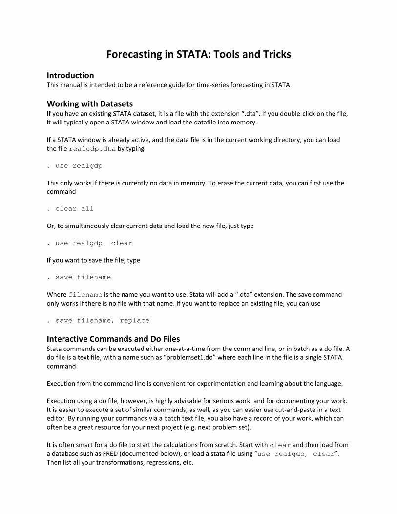
To obtain a specific percentile, e.g. 2.5%, here are two options. One is to use the qreg (quantile regression) command . qreg wage, quantile(.025) This estimates an intercept-only quantile regression. The estimated intercept (in this case 5.5) is the 2.5% percentile of the wage distribution. The second method uses the _pctile command . _pctile wage, p(2.5 97.5) . return list This calculates the 2.5% and 97.% percentiles (which are 5.5 and 48.08 in this example) Histogram, Density, Distribution, and Scatter Plots To plot a histogram of the variable wage . histogram wage

0.0

2.0

4.0

6D

ensi

ty

0 50 100 150 200 250wage

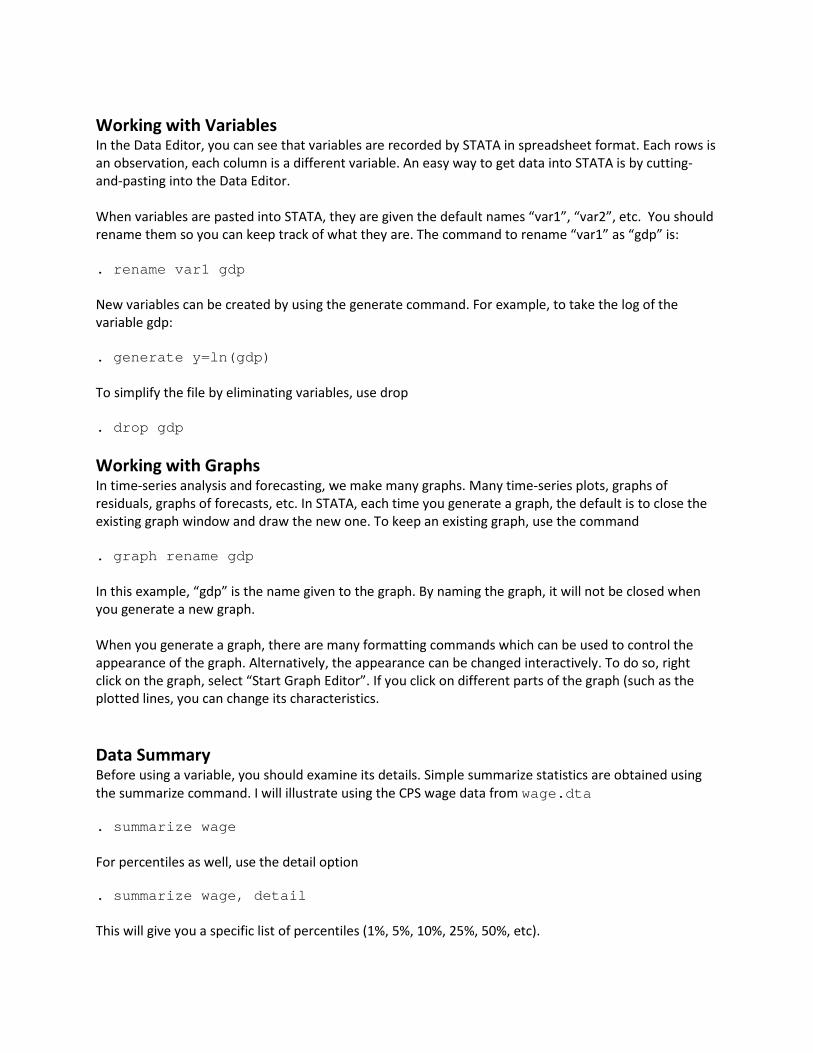
A smoother version is obtained by a kernel density estimator. Informally, you can think of it as a “smoothed histogram”, but it is more accurately an estimate of the density. Statistically-trained people prefer density estimates to histograms, non-trained individuals tend to understand histograms better . kdensity wage

0.0

2.0

4.0

6D

ensi

ty

0 50 100 150 200 250wage

kernel = epanechnikov, bandwidth = 1.1606

Kernel density estimate

The default in STATA is for the density to be plotted over the range from the smallest to largest values of the variable, in this case 0 to 231. Consequently on this graph it is difficult to see the detail. To focus in on part of the range, you need to use a different command. For example, to plot the density on the range [0,60] use

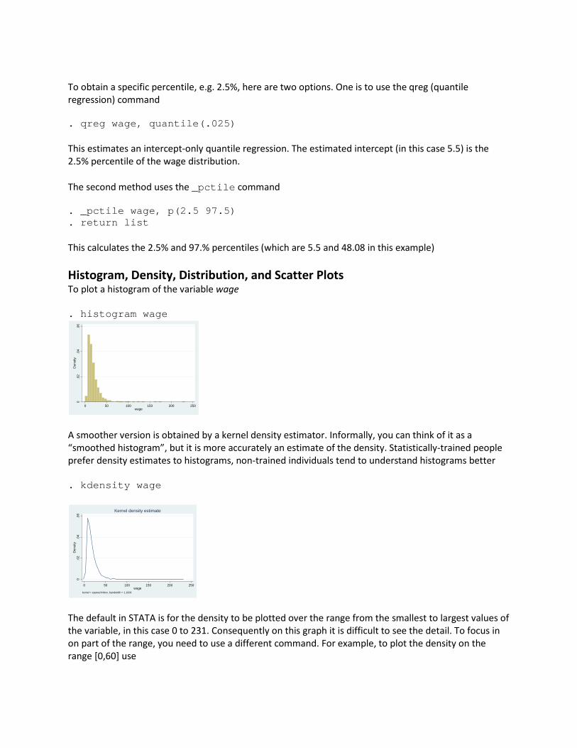
. twoway kdensity wage, range(0,60)

0.0

2.0

4.0

6kd

ensi

ty w

age

0 20 40 60x

For a cumulative distribution function, use cumul function, which creates a new variable, and then you can plot it using the line command . cumul wage, gen(f) . line f wage if wage<=60, sort

0.2

.4.6

.81

f

0 20 40 60wage

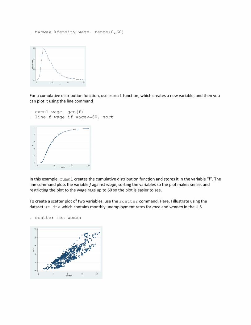
In this example, cumul creates the cumulative distribution function and stores it in the variable “f”. The line command plots the variable f against wage, sorting the variables so the plot makes sense, and restricting the plot to the wage rage up to 60 so the plot is easier to see. To create a scatter plot of two variables, use the scatter command. Here, I illustrate using the dataset ur.dta which contains monthly unemployment rates for men and women in the U.S. . scatter men women

24

68

1012

men

2 4 6 8 10women

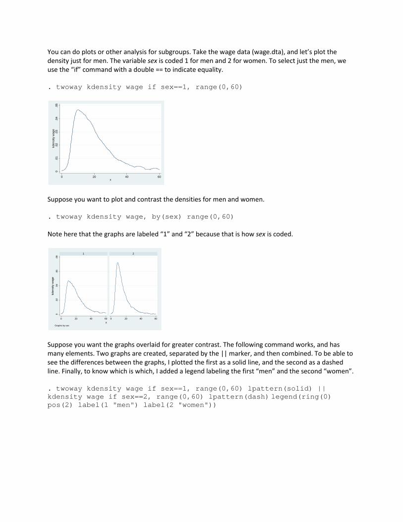
You can do plots or other analysis for subgroups. Take the wage data (wage.dta), and let’s plot the density just for men. The variable sex is coded 1 for men and 2 for women. To select just the men, we use the “if” command with a double == to indicate equality. . twoway kdensity wage if sex==1, range(0,60)

0.0

1.0

2.0

3.0

4.0

5kd

ensi

ty w

age

0 20 40 60x

Suppose you want to plot and contrast the densities for men and women. . twoway kdensity wage, by(sex) range(0,60) Note here that the graphs are labeled “1” and “2” because that is how sex is coded.

0.0

2.0

4.0

6.0

8

0 20 40 60 0 20 40 60

1 2

kden

sity

wag

e

xGraphs by sex

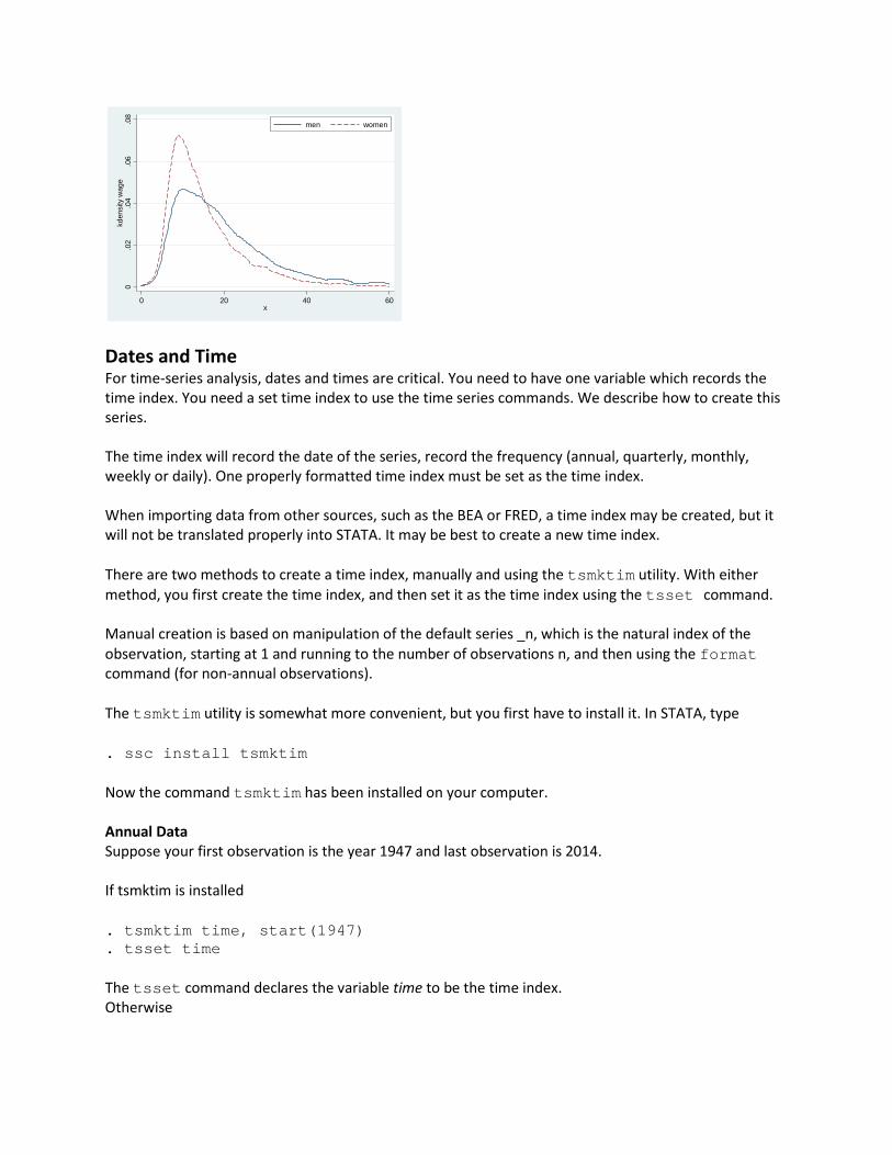
Suppose you want the graphs overlaid for greater contrast. The following command works, and has many elements. Two graphs are created, separated by the || marker, and then combined. To be able to see the differences between the graphs, I plotted the first as a solid line, and the second as a dashed line. Finally, to know which is which, I added a legend labeling the first “men” and the second “women”. . twoway kdensity wage if sex==1, range(0,60) lpattern(solid) || kdensity wage if sex==2, range(0,60) lpattern(dash) legend(ring(0) pos(2) label(1 "men") label(2 "women"))

0.0

2.0

4.0

6.0

8kd

ensi

ty w

age

0 20 40 60x

men women

Dates and Time For time-series analysis, dates and times are critical. You need to have one variable which records the time index. You need a set time index to use the time series commands. We describe how to create this series. The time index will record the date of the series, record the frequency (annual, quarterly, monthly, weekly or daily). One properly formatted time index must be set as the time index. When importing data from other sources, such as the BEA or FRED, a time index may be created, but it will not be translated properly into STATA. It may be best to create a new time index. There are two methods to create a time index, manually and using the tsmktim utility. With either method, you first create the time index, and then set it as the time index using the tsset command. Manual creation is based on manipulation of the default series _n, which is the natural index of the observation, starting at 1 and running to the number of observations n, and then using the format command (for non-annual observations). The tsmktim utility is somewhat more convenient, but you first have to install it. In STATA, type . ssc install tsmktim Now the command tsmktim has been installed on your computer. Annual Data Suppose your first observation is the year 1947 and last observation is 2014. If tsmktim is installed . tsmktim time, start(1947) . tsset time The tsset command declares the variable time to be the time index. Otherwise

. generate time=1947+_n-1

. tsset time This creates a series time whose first value is 1947 and runs to 2014. Quarterly Data STATA stores the time index as an integer series. It uses the convention that the first quarter of 1960 is 0, the second quarter of 1960 is 1, the first quarter of 1961 is 4, etc. Dates before 1960 are negative integers, so that the fourth quarter of 1959 is -1, the third is -2, etc. When formatted as a date, STATA displays quarterly time periods as “1957q2”, meaning the second quarter of 1957. (Even though STATA stores the number “-11”, the eleventh quarter before 1960q1.) STATA uses the formula “tq(1957q2)” to translate the formatted date “1957q2” to the numerical index “-11”. Suppose that your first observation is the third quarter of 1947. You can generate a time index for the data set by the commands . generate time=tq(1947q3)+_n-1 . format time %tq . tsset time This creates a variable time with integer entries, normalized so that 0 occurs in 1960q1. The format command formats the variable time with the time-series quarterly format. The “tq” refers to “time-series quarterly”. The tsset command declares that the variable time is the time index. You could have alternatively typed . tsset time, quarterly to tell STATA that it is a quarterly series, but it is not necessary as time has already been formatted as quarterly. Now, when you look at the variable time you will see it displayed in year-quarter format. Alternatively, . tsmktim time, start(1947q1) . tsset time By specifying that the start date is 1947q1, tsmktim understands that the variable time should be formatted as a quarterly time series Monthly Data Monthly data is similar, but with “m” replacing “q”. STATA stores the time index with the convention that 1960m1 is 0. To generate a monthly index starting in the second month of 1962, use the commands . tsmktim time, start(1962m2) . tsset time Alternatively

. generate time=tm(1962m2)+_n-1 . format time %tm . tsset time Weekly Data Weekly data requires a bit more attention. If the data are formatted as a weekly time series, STATA will handle it by specifying that there are precisely 52 weeks each year, and will denote the observations by weekly numbers, that is, week 1 through week 52. If this is appropriate use the following. The format is similar to quarterly and monthly, but with “w” instead of “q” and “m”, and the base period is 1960w1. For a series starting in the 7th week of 1973, use the commands . tsmktim time, start(1973w7) . tsset time Or alternatively . generate time=tw(1973w7)+_n-1 . format time %tw . tsset time The limitation of the weekly format is that it does not correspond to most series. Leap years have an extra day, throwing off the 52-week format. For series which are tied to specific days, typically Fridays for end-of-week, it is better to format the data as daily, but with only every 7th day recorded. This can be done as follows. For a weekly series starting on January 6, 1950, use . generate time=td(06jan1950)+(_n-1)*7 . format time %td . tsset time, daily delta(7) The first line creates a series starting on Jan 6 with even increments of 7 days. The second line formats it as daily data. The third declares time as time index, and formatted as daily, with the important modification that the increment between observations is 7 days. Daily Data Daily data is stored by dates. For example, “01jan1960” is Jan 1, 1960, which is the base period. To generate a daily time index staring on April 18, 1962, use the commands . tsmktim time, start(18apr1962) . tsset time Alternatively, . generate time=td(18apr1962)+_n-1 . format time %td . tsset time

Loading Data in STATA from FRED One simple way to obtain data is from the Federal Reserve Bank of St Louis Economic Data page, known as FRED, at http://research.stlouisfed.org/ You need to first install the freduse utility. In STATA, type . ssc install freduse If you know the name of the series you want, you can then directly import them into STATA using the freduse command. For example, quarterly real GDP is GDPC1, and quarterly real GDP percent change from previous period is A191RL1Q225SBEA. To import these two into STATA, type . freduse GDPC1 A191RL1Q225SBEA The exact spelling, including capitalization, is required. If the command is successful, the variables are now in the STATA file, with these names. Also two time indices are included, date and daten. The date formats are off, however, so I recommend creating a new date index (as described above) and setting it to be the time index. To learn the desired name of the series you want (you want a precise series, so do not guess!) you need go to the FRED website. From the main site, go to FRED Economic Data/Categories, and then browse. For example, to find the GDP variables you would go to National Accounts/National Income & Product Accounts/GDP and then click on the names of the series you want. The FRED name is in the second line, after the seasonality. Copy and paste this label into the STATA freduse command. After loading the data into STATA, you should verify that the data loaded correctly. Examine the entries using the Data Editor. Make a time series plot (see below). Also, change the variable names into something more convenient for use. Loading Data into STATA by Pasting If the data you want is not in FRED, you will need to load it in yourself. One relatively ease method is to use copy and paste, where you paste the data as a table, or series by series, into the Data Editor. To do this, open the data editor (Data/Data Editor/Edit). Copy the data from your source file (e.g. an Excel file) and paste into the Data Editor window. For pasting to work the best, the data should be organized as a table, with each row a single time-series observation, in sequence from first observation to last, and each column a single variable. For example, the observations are quarterly from 1947q1 to 2014q4, and the variables are GDP growth, CPI inflation rate, and consumption growth rate. If successful, the variables will be given default names of the form var1, var2, etc. You should change the names so that they are interpretable. If you have an existing time-series data set (with a time index) you can paste a new series into the Data Editor, but the observations will need to be a subset of the existing dates. If the new data observations go beyond the existing sample, you will need to extend the sample (using the tsappend command described below).

Pasting works best if the source data is in a spreadsheet such as Excel. Then the observations and variables are very cleanly laid out on a grid. It is therefore often the best strategy to first copy a data source into Excel, manipulate if necessary to make it the proper format, and then copy and paste into STATA. Non-Standard Data Formats Some quarterly and monthly data are available as tables where each row is a year and the columns are different quarters or months. If you paste this table into STATA, it will treat each column (each month) as a separate variable. This is not what you want! You can use STATA to rearrange the data into a single column, but you have to do this for one variable at a time. I will describe this for monthly data, but the steps are the same for quarterly. After you have pasted the data into STATA, suppose that there are 13 columns, where one is the year number (e.g. 1958) and the other 12 are the values for the variable itself. Rename the year number as year, and leave the other 12 variables listed as var2 etc. Then use the reshape command . reshape long var, i(year) j(month) Now, the data editor should show three variables: year, month and var. STATA has resorted the observations into a single column. You can drop the year and month variables, create a monthly time index, and rename var to be more descriptive. In the reshape command listed above, STATA takes the variables which start with var and strips off the trailing numbers and puts them in the new variable month. It uses the existing variable year to group observations. Data Organized in Rows Some data sets are posted in rows. Each row is a different variable, and each column is a different time period. If you cut and paste a row of data into STATA, it will interpret the data as a single observation with many variables. One method to solve this problem is with Excel. Copy the row of data, open a clean Excel Worksheet, and use the Paste Special Command. (Right click, then “Paste Special”.) Check the “Transpose” option, and “OK”. This will paste the data into a column. You can then copy and paste the column of data into the STATA Data Editor. Cleaning Data Pasted into STATA Many data sets posted on the web are not immediately useful for numerical analysis, as they are not in calendar order, or have extra characters, columns, or rows. Before attempting analysis, be sure to visually inspect the data to be sure that you do not have nonsense. Examples

• Data at the end of the sample might be preliminary estimates, and be footnoted or marked to indicate that they are preliminary. You can use these observations, but you need to delete all characters and non-numerical components. Typically, you will need to do this by hand, entry-by-entry.

• Seasonal data may be reported using an extra entry for annual values. So monthly data might be reported as 13 numbers, one for each month plus 1 for the annual. You need to delete the annual variable. To do this, you can typically use the drop command. For example, if these entries are marked “Annual”, and you have pasted this label into var2, then

. drop if var2==”Annual” This deletes all observations for which the variable var2 equals “Annual”. Notices that this command uses a double equality “==”. This is common in programming. The single equality “=” is used for assignment (definition), and the double equality “==” is used for testing. Time-Series Plots The tsline command generates time-series plots. To make plots of the variable gdp, or the variables men and women . tsline gdp

-10

010

20R

eal G

ross

Dom

estic

Pro

duct

1950q1 1960q1 1970q1 1980q1 1990q1 2000q1 2010q1time

. tsline men women Time-series operators For a time-series y L. lag y(t-1) Example: L.y L2. 2-period lag y(t-2) Example: L2.y F. lead y(t+1) Example: F.y F2. 2-period lead y(t+2) Example: F2.y D. difference y(t)-y(t-1) Example: D.y

D2. double difference (y(t)-y(t-1))- (y(t-1)-y(t-2)) Example: D2.y S. seasonal difference y(t)-y(t-s), where s is the seasonal frequency (e.g., s=4 for quarterly) Example: S.y S2. 2-period seasonal difference y(t)-y(t-2s) Example: S2.y Regression Estimation To estimate a linear regression of the variable y on the variables x and z, use the regress command . regress y x z The regress command reports many statistics. In particular,

• The number of observations is at the top of the small table on the right • The sum of squared residuals is in the first column of the table on the left (under SS), in the row

marked “Residual”. • The least-squares estimate of the error variance is in the same table, under “MS” and in the row

“Residual”. The estimate of the error standard deviation is its square root, and is in the right table, reported as “Root MSE”.

• The coefficient estimates are reported in the bottom table, under “Coef”. • Standard errors for the coefficients are to the right of the estimates, under “Std. Err.”

In some time-series cases (most importantly, trend estimation and h-step-ahead forecasts), the least-squares standard errors are inappropriate. To get appropriate standard errors, use the newey command instead of regress. . newey y x z, lag(k) Here, “k” is an integer, meaning number of periods, which you select. It is the number of adjacent periods to smooth over to adjust the standard errors. STATA does not select k automatically, and it is beyond the scope of this course to estimate k from the sample, so you will have to specify its value. I suggest the following. In h-step-ahead forecasting, set k=h. In trend estimation, set k=4 for quarterly and k=12 for monthly data. Intercept-Only Model The simplest regression model is intercept-only, y=b0+e. This can be estimated by the regress or newey command . regress y . newey y, lag(k) The estimated intercept is the sample mean of y. While this could have been calculated using other methods, such as the summarize command, using the regress or newey command is useful as then afterwards you can use postestimation commands, including predict.

Regression Fit and Residuals To calculate predicted values, use the predict command after the regress or newey command . predict p This creates a variable p of the fitted values x’beta. To calculate least-squares residuals, after the regress or newey command . predict e, residuals This creates a variable e of the in-sample residuals y-x’beta. You can then plot the fit versus actual values, and a residual time-series . tsline y p . tsline e The first plot is a graph of the variables y and p, assuming that y is the dependent variable, and p are the fitted values. The second plot is a graph of the residuals against time. Dummy Variables Indicator variables, known as dummy variables, can be created using generate. One purpose is to create sub-periods and regimes. For example, to create a dummy variable equaling “0” for observations before 1984, and equaling “1” for monthly observations starting in 1984 . generate d=(t>=tm(1984m1)) In this example, the time index is t. The command tm(1984m1)converts the date format 1984m1 into an integer value. The new variable is d, and equals “0” for observations up to 1983m12, and equals “1” for observations starting in 1984m1. To create a dummy variable equaling “1” for quarterly observations between 1990q1 and 1998q4, and “0” otherwise, (and the time index is t) use . generate d=(t>=tq(1990q1))*(t<=tq(1998q4)) This command essentially generated two dummy variables and then multiplied them to create the variable d. Changing Intercept Model We can allow the intercept of a model to change at a known time period we simply add a dummy variable to the regression. For example, if t is the time index, the data are monthly and we want a change in mean starting in the 7th month of 1987, . generate d=(t>=tm(1987m7))

. regress y d The generate command created a dummy variable for the second time period. The regress command estimated an intercept-only model allowing a switch in the intercept in July 1987. The estimated “constant” is the intercept before July 1987. The coefficient on d is the change in the intercept. Time Trend Model To estimate a regression on a time trend only, use regress or newey with the time index as a regressor. If the time index is t . regress y t Trends with Changing Slope Here is how to create a trend which changes slope at a specific date (for concreteness 1984m1). Use the generate command to create a dummy for the period starting at 1984m1, and then interact it with a trend normalized to be zero at 1984m1: . generate d=(t>=tm(1984m1)) . generate ts=d*(t-tm(1984m1)) The new variable ts is zero before 1984, and then is a linear trend after that. Then regress the variable of interest on t and ts: . regress t ts The coefficient on t is the trend before 1984. The coefficient on ts is the change in the trend. If you want there to be a jump as well as a change in slope at 1984m1, then include the dummy d . regress t d ts Expanding the Dataset Before Forecasting When you have a set of time-series observations, STATA typically records the dates as running from the first until the last observation. You can check this by looking at the data in the Data Editor. But to forecast a date out-of-sample, these dates need to be in the data set. This requires expanding the dataset to include these dates. This is done by the tsappend command. There are two formats . tsappend, add(12) This command adds 12 dates to the end of the sample. If the current final observation is 2009m12, the command adds 2010m01 through 2010m12. If you look at the data using the Data Editor, you will see that the time index has new entries, through 2010m12, but the other variables are missing. Missing values are indicated by a period “.”. The other format which accomplishes the same task is

. tsappend, last (2010m12) tsfmt(tm) This command adds observations so that the last observation is 2010m12, and that the formatting is monthly. For quarterly data, to add observations up to 2010q4 the command is . tsappend, last (2010q4) tsfmt(tq) Point Forecasting Out-of-Sample The predict command can be used for point forecasting, so long as the regressors are available. The dataset first needs to be expanded as previously described, and the regression coefficients estimated using either the regress or newey commands. The command . predict p This creates a series p of predicted values, both in-sample and out-of-sample. To restrict the predicted values to be in-sample, use . predict p To restrict the predicted values to in-sample observations (for quarterly data with time index t and the last in-sample observation 2009m12) . predict p if t<=tm(2009m12) To restrict the predicted values to out-of-sample (for monthly data with the last in-sample 2009m12) . predict yp if t>tm(2009m12) If the observations, in-sample predictions, and out-of-sample predictions are y, p, and yp, they can be plotted together, but as three distinct elements, as . tsline y p yp . tsline y p yp if t>tm(2000m12) The second command restricts the plot to observations after 2000, which is useful if you wish to focus in on the forecast period (the example is for quarterly data). Standard Deviation of Forecast The “standard deviation of a forecast” is an estimate of the standard deviation of the forecast error. For a regression forecast it can be calculated in STATA using the stdf option to the predict command . regress y x z . predict s, stdf This creates a variable s for the forecast period whose entries are the standard deviation of the forecast.

Normal Forecast Intervals These are based on the normal approximation to the forecast error. You need the point forecasts and the standard errors of the forecast, both computed using the predict command. You first need to estimate the forecast and save the forecast. Suppose you are forecasting the monthly variable y given the regressors x and z, the in-sample ends in 2009m12. We make the following commands . regress y x z . predict p if t<=tm(2009m12) . predict yp if t>tm(2009m12) . predict s if t>tm(2009m12), stdf Now you multiply the standard deviation of the forecast by a standard normal quantile and add to the point forecast . generate yp1=yp-1.645*stdf . generate yp2=yp+1.645*stdf These commands create two series for the forecast period, which equal the endpoints of a forecast interval with 90% coverage. (-1.645 and 1.645 are the 5% and 95% quantiles of the normal distribution). Empirical Forecast Intervals To make an interval forecast, you need to estimate the quantiles of the residuals of the forecast equation. To do so, you first need to estimate the forecast and save the forecast. Suppose you are forecasting the monthly variable y given the regressors x and z, the in-sample ends in 2009m12. We make the following commands . regress y x z . predict p if t<=tm(2009m12) . predict yp if t>tm(2009m12) . predict e, residuals Now we want to calculate the 25% and 75% quantiles of the residuals e. This can be accomplished using what is called quantile regression with just an intercept. The STATA command is qreg. The format is similar to regress, but you have to tell STATA the quantile you want to estimate. . qreg e, quantile(.25) This command computes the 25% quantile regression of e on an intercept (as no regressors are specified). The “Coef.” Reported in the table is the .25 quantile of e. Now you can compute the out-of-sample values, and add them to the point forecast yp to create the lower part of the forecast interval . predict q1 if t>tm(2009m12) . generate yp1=yp+q1 The predict command uses the last estimation command – in this case qreg – to compute the forecast. In this case it is computing the out-of-sample .25 quantile of e. You can repeat this for the upper forecast interval endpoint.

. qreg e, quantile(.75) . predict q2 if t>tm(2009m12) . generate yp2=yp+q2 The variables yp1 and yp2 are the out-of-sample forecast interval endpoints for y. You can plot the data together with the out-of-sample point and interval forecasts, e.g. . tsline y yp yp1 yp2 if t>tm(2000m12) For a fan chart, you repeat this for multiple quantiles. Conditional Forecast Intervals The qreg command makes it easy to compute the forecast interval endpoints conditional on regressors. This is a quite advanced technique, so I do not recommend it without care. But this is how it can be done. As in the previous section, suppose you are forecasting y given x and z, have forecast residuals e, and out-of-sample point forecast yp. Now you want out-of-sample conditional quantiles of e given some regressor x. You can use the commands for the .25 quantile . qreg e x, quantile(.25) . predict q1 if t>tm(2009m12) . generate yp1=yp+q1 and similarly for the .75 quantile. This method models the quantiles of e as functions of x. This can be useful when the spread (variance) of the distribution changes over time. Autocorrelation Plots To create an autocorrelation plot of the variable ur, . ac ur

-0.5

00.

000.

501.

00Au

toco

rrela

tions

of u

r

0 10 20 30 40Lag

Bartlett's formula for MA(q) 95% confidence bands

The shaded area are Bartlett confidence bands for testing that the autocorrelation is zero. Thus if the lines break out of the shaded area, we reject that the series is not autocorrelated. MA estimation

To estimate a MA(q) model for the . arima ur, arima(0,0,q) AR(1) estimation To estimate a AR(1) model for the variable ur, . regress ur L.ur AR(2) estimation To estimate a AR(2) model for the variable ur, . regress ur L.ur L2.ur Or alternatively . regress ur L(1/2).ur

AR(k) estimation To estimate a AR(k) model for the variable ur, say an AR(8) . regress ur L(1/8).ur Simulating an AR process To simulate a variable with 100 observations from the AR(2) model y(t)=1.35y(t-1)-.45y(t-2)+e(t) where e(t) is N(0,1), . set obs 100 . gen t=_n . tsset t . gen e=rnormal() . gen y=e . replace y=1.35*L.y-.45L2.y+e if t>2 Seasonality With seasonal (quarterly or monthly, typically) data, you may want to include dummy variables indicating the quarter or month. If the time index is time and is formatted as a time index, you can determine the period using the commands . generate m=month(dofm(time)) . generate q=quarter(dofq(time)) . generate w=week(dofw(time)) for monthly, quarterly, and weekly data respectively. Then m will equal 1 for January, 2 for February, etc.

To create monthly dummies, supposing m is the month as created above, then to create a dummy variable m1 to indicate that the month is January, you can use . generate m1=(m==1) You can then repeat this for m2 through m12. For a regression of a variable y on 11 seasonal dummies, you can then use . regress y m1 m2 m3 m4 m5 m6 m7 m8 m9 m10 m11 You do not include m12 as it is collinear with the intercept. Alternatively, you could use . regress y b12.m Similar commands are used for quarterly and weekly. Standard Error Calculation For “old-fashioned standard errors . regress y x For standard errors which are robust to conditional heteroskedasticity . regress y x, r For standard errors which are robust to serial correlation, for some positive integer k . newey y x, lag(k)