forecasting inflation james h. stock mark w. watson http ... · forecasting inflation james h....
TRANSCRIPT

NBER WORKING PAPER SERIES
FORECASTING INFLATION
James H. StockMark W. Watson
Working Paper 7023http://www.nber.org/papers/w7023
NATIONAL BUREAU OF ECONOMIC RESEARCH1050 Massachusetts Avenue
Cambridge, MA 02138March 1999
We have benefited from comments by Guido Kuersteiner, Brian O'Reilly, a referee, andparticipants at theStudienzendrum Gerzensee conference on the Return of the Phillips Curve. This researchwas supported byNational Science Foundation grant SBR-973 0489. The views expressed in this paper are those of the authorsand do not reflect those of the National Bureau of Economic Research.
© 1999 by James H. Stock and Mark W. Watson. All rights reserved. Short sections of text, not to exceedtwo paragraphs, may be quoted without explicit permission provided that full credit, including © notice,is given to the source.

Forecasting InflationJames H. Stock and Mark W. WatsonNBER Working Paper No. 7023March 1999JELNo. E31,C32
ABSTRACT
This paper investigates forecasts of U.S. inflation at the 12-month horizon. The starting point
is the conventional unemployment rate Phillips curve, which is examined in a simulated out of
sample forecasting framework. Inflation forecasts produced by the Phillips curve generally have
been more accurate than forecasts based on other macroeconomic variables, including interest rates,
money and commodity prices. These forecasts can however be improved upon using a generalized
Phillips curve based on measures of real aggregate activity other than unemployment, especially a
new index of aggregate activity based on 61 real economic indicators.
James H. Stock Mark W. WatsonKennedy School of Government Woodrow Wilson SchoolHarvard University Princeton UniversityCambridge, MA 02138 Princeton, NJ 08544and NBER and NBER

1. Introduction
The Phillips curve has played a prominent role in empirical macroeconomics in the U.S.
over the past four decades. As a tool for forecasting inflation, it is widely regarded as stable,
reliable, and accurate, at least compared to the alternatives; Alan Blinder, when Vice Chair of
the Board of Governors of the U.S. Federal Reserve System, called it the "clean little secret" of
empirical macroeconomics.
This paper reassesses the use of the Phillips curve for forecasting price inflation. We focus
on three questions. First, has the U.S. Phillips curve been stable? If not, what are the
implications of the instability for forecasting future inflation? Second, the Phillips curve is
conventionally specified in terms of unemployment, but at a conceptual level other measures of
economic activity could be used instead. Do these alternative Phillips curves provide better
forecasts of inflation than the unemployment rate Phillips curve? Third, these variables are, of
course, a small subset of the many macroeconomic variables that are potentially useful for
forecasting inflation. For example, monetary theories of inflation and the theory of the term
structure of interst rates suggest alternative frameworks for forecasting inflation. How do
inflation forecasts from the Phillips curve stack up against time series forecasts made using
interest rates, money, and other series? Put baldly, is it time for inflation forecasters to move
beyond the Phillips curve?
The focus of this paper is on forecasting price inflation using monthly data for the U.S.
from 1959:1 to 1997:9. Attention is restricted to forecasts of inflation over a twelve-month
horizon. All forecasting comparisons are performed using a simulated out-of-sample
methodology, that is, all models are estimated with data that is dated prior to forecast period.
This empirical analysis suggests some answers to these questions.
—1—

First, we find that there is statistical evidence that the parameters of the Phillips curve, as
conventionally specified, have changed over this period. The major source of instability seems
to be changes in the contribution of lags of inflation in the Phillips curve. While this instability
is statistically significant, it appears to be quantitatively small.1
Second, Phillips curves specified with alternative measures of real economic activity can
provide forecasts with smaller mean squared errors than those from unemployment-based
Phillips curves. For example, Phillips curves that use housing starts, capacity utilization or the
rate of growth of manufacturing and trades sales produce forecasts that are generally more
accurate than forecasts constructed from Phillips curves using the unemployment rate.
Third, it is possible to improve upon traditional Phillips curve forecasts by using alternative
economic indicators to forecast inflation. The investigation here casts a wide net: we consider
forecasts of inflation based on 189 additional economic indicators. Several conclusions emerge.
Although there are theoretical reasons to expect interest rates and interest rate spreads to be
useful for predicting inflation, forecasts based on these variables fail to improve on Phillips
curve forecasts, at least at the one year horizon. The evidence on nominal money is less clear
cut: models that add indexes of the money supply to the Phillips curve provide marginal
improvements for some sample periods and some measures of inflation, but they lead to a
serious deterioration in accuracy for forecasts of inflation based on the consumer price index
during the 1970's and early 1980's. Commodity prices do not improve inflation forecasts at the
12-month horizon. The only variables that consistently improve upon Phillips curve forecasts
are measures of aggregate activity, and the best of these is a new index of 61 indicators of
aggregate activity. These alternative forecasts, when combined with Phillips curve forecasts,
produce forecasting gains that are both statistically and economically significant.
These results lead us to conclude that the unemployment rate Phillips curve can play a
useful role in forecasting inflation, but that relying on it to the exclusion of other forecasts is a
-2-

mistake. Forecasting relations based on other measures of aggregate activity can perform as
well or better than those based on unemployment, and combining these forecasts produces still
further improvements.
The remainder of the paper is organized as follows. In section 2, we examine the stability
of standard specifications of the Phillips curve. In section 3, Phillips curves based on
alternative measures of aggregate activity are considered. In section 4, forecasts of inflation
from the Phillips curve are compared with forecasts based on our full set of 189 economic
indicators. Section 5 considers multivariate forecasts of inflation that use all 189 indicators.
The results in sections 2-5 maintain the conventional assumption that inflation is integrated of
order 1 (is 1(1)), and the robustness of our results to this assumption is investigated in section 6.
Section 7 concludes.
2. Stability of the U.S. Phillips Curve, 1959-1997
Conventional specifications of the Phillips curve relate the change of inflation to past values
of the unemployment gap (the difference between the unemployment rate and the NAIRU), past
changes of inflation, and current and/or past values of variables that control for various supply
shocks.2 Because we are interested forecasting, we adopt this framework with two
modifications: the dependent variable is the change in the inflation rate over periods longer than
the sampling frequency, and supply shocks measures are not included in the equation. The first
modification allows us to use the estimated equation directly for multiperiod (12-month-ahead)
forecasting. Supply shock measures are omitted because preliminary results (not reported here)
indicated that the forecasting performance of models that included these variables (the relative
price of food and energy and the Nixon price control variable as in Gordon (1982, 1997)) is
-3-

worse, on a simulated out of sample basis, than the corresponding models in which these
variables are excluded. This is not surprising: although the supply shock variables are
statistically significant in full-sample specifications with unemployment, in a simulated out of
sample setting their coefficients are poorly estimated for much of the sample and this produces
poor out of sample forecasts. This is consistent with these supply shock measures being
identified as useful in unemployment-based Phillips curves based on ex-post analysis.
The Phillips curve specification used in this paper is,
(1) t+ht = + 13(L)ut + + et+h
where =(1200/h)ln(PtIPth) is the h-period inflation in the price level P, reported at an
annual rate; =l2OO*ln(Pt/Pt1) is monthly inflation at an annual rate; u is the
unemployment rate; and j3(L) and 'y(L) are polynomials in the lag operator L.
This specfication imposes two important restrictions. The first is that inflation is integrated
of order one (is 1(1)). The specification (1) is equivalent to a specification with +h as the
left hand variable and replacing y(L)iirt with, say, ,.L(L)lrt, subject to the restriction that L(1) =1.
Thus, for h= 12, this specification can be thought of as predicting inflation over the next twelve
months using a distributed lag of current and past inflation, subject to the restiction that the
distributed lag coefficients sum to one. Modeling U.S. price inflation as 1(1) is standard in this
literature, and as we discuss below, is consistent with recursive unit-root tests of various
inflation series over most of the sample period. The robusmess of the main substantive results
to relaxing the unit root assumption is examined in the penultimate section of this paper.
The second restriction imposed in (1) is that the NAIRU is constant. To see this, note that
the Phillips curve is conventionally written as
-4-

(2) t+ht = 13(L)(ut-iit) + + et+h
where u is the NAIRU. When Ut is time invariant so that then (2) can be written as
(1) with the constant term 4=-/3(1)u. There is a large recent literature on the constancy of the
NAIRU, and the constancy of the Phillips curve more generally (see Gordon (1997a, 1998),
King and Watson (1994), Shimer (1998), Staiger, Stock and Watson (1997a, 1997b), Stock
(1998)). This research documents instability in the coefficients of specifications like (1) using
postwar data for the U.S. Instability in (1) has obviously important implications for
forecasting, and thus we will examine stability of the coefficients in (1) before discussing the
forecasting performance of the Phillips curve.
Our estimates use monthly data for the U.S., 1959:1-1997:9. Figure 1 plots annual inflation
rates, 7rF, for two closely watched U.S. monthly price indexes: the consumer price index
(CPI-U; the mnemonic in the figure is PUNEW3) and the personal consumption expenditure
(PCE) deflator (GMDC in the figure). Although the two measures of inflation are generally
similar, there are marked differences in 1975 and 1980 (when CPI inflation was much higher
than PCE inflation) and in 1983 and 1985 (when CPI inflation was much lower than PCE
inflation). The causes of the differences in the series are well known: the CPI is essentially a
Laspeyres index which uses a fixed basket to weight its constituent prices, while the PCE
deflator uses chain weighting; the CPI data are not historically revised when methods or data
change, while the PCE deflator is subject to revision. Because a major change in the CPI
occurred in 1983, when the owner-occupied housing component was changed, results will also
be presented for CPI inflation with housing services eliminated (PUXHS). Two unemployment
rates are considered: the total civilian unemployment rate (LHUR), and the unemployment rate
for males ages 25-54 (LHMU25). The latter series is included to control for potential
demographic shifts that could affect the stability of the coefficients, in particular the large
increase in female labor force participation rates over this period.
-5-

Several tests for the stability of the parameters in (1) were performed. All are variants of
the Quandt (1960) likelihood ratio (QLR) procedure, which tests for a single breakpoint in the
regression. The tests were implemented as the maximum of HAC-robust Wald statistics for
shifts in the coefficients over all possible break dates in the middle 70% of the sample; p-values
for the statistics are computed using the approximation given in Hansen (1997). Results are
shown in Table 1 for regressions estimated over horizons h= 1 and h= 12. The first statistic
(QLR1) tests for the constancy of all the parameters in (1), The next statistic (QLR 13) tests
for stability of the constant term (and hence the NAIRU) together with the coefficients on the
lags of the unemployment rate (13(L)) assuming that the coefficients in y(L) are constant.
Similarly QLR tests for the stability of the coefficients on lagged changes in inflation (y(L))
assuming and 13(L) are constant. For each combination of price and unemployment rate data,
the number of lags in j3(L) and y(L) were chosen separately by the Bayes information criterion
(BIC) over the full sample, where in both cases the number of lags was permitted to be between
0 and 11.
The QLR statistics in Table 1 indicate statistically significant evidence of instability in
these empirical Phillips curves. This instability appears to be concentrated in the coefficients
on lagged inflation: while the QLRall and QLR7 statistics are statistically significant, the
QLR statistics provide far less evidence of instability in the NAIRU and in the effect of
unemployment on future values of inflation. Importantly, while the instability in y(L) is
statistically significant, it does not seem to be quantitatively large, particularly in its effect on
12-month ahead forecasts. Figure 2 plots estimates of the accumulated values of [1-Ly(L)i
(the impulse responses from et to future values of holding the unemployment rate constant)
estimated over the first and second half of the samples for the CPI and PCE deflator using
LHUR. These impulse responses are broadly similar across the two sample periods, and most of
the differences occur for horizons less than 12 months. This evidence is consistent with results
-6-

presented in King and Watson (1994), who found statistically significant shifts in the
coefficients of a bivariate VAR fit to postwar U.S. inflation and unemployment data, but found
that these shifts had little effect on the forecasts produced by the VAR.
In the forecasting experiments that we carry out in later sections we will ignore this
instability, except to the extent that it is captured in recursive estimates of the regression
coefficients, We do this for two reasons. First, figure 2 shows that the instability is small, so
that gains from incorporating this instability are likely to be modest at best. In fact, when
instability is small, existing statistical forecasting methods that incorporate parameter instability
(rolling regression, TVP models, etc.) perform no better than recursive least squares, and in
many cases perform significantly worse (for some empirical evidence, see Stock and Watson
[1996]). Second, this instability has been identified in a full-sample analysis, and incorporating
it into the models is inconsistent with the simulated real-time methodology of the forecasting
exercise.
3. Inflation Forecasts Based on Measures of Aggregate Real Activity
Although the Phillips curve is typically specified in terms of the deviation of unemployment
from its natural rate, more generally it is a relation between inflation and aggregate real
activity. This section compares the forecasting performance of the conventional unemployment
rate Phillips curve to generalized Phillips curves that use other measures of aggregate activity.
The forecasting models used here are analogous to (1) except that the alternative indicator,
x, replaces unemployment:
(3) +ht = + (L)xt + 7(L)t + et+h.
-7-

In (3), it is assumed that has already been transformed so that it is 1(0). This assumes that
inflation and the alternative demand measure are not cointegrated, an assumption that is
theoretically and empirically plausible for real activity measures (robustness to this assumption is
examined in section 6.) Specification (3) mirrors specification (1). The constant intercept
implies that, under (3), the "natural rate of xi" is constant.
Seven alternative measures of aggregate activity are considered: industrial production (IP),
real personal income (GMPYQ), total real manufacturing and trade sales (MSMTQ), the number
of employees on nonagricultural payrolls (LPNAG), the capacity utilization rate in
manufacturing (IPXMCA), and housing starts (HSBP). We also consider the unemployment rate
for males ages 25 to 54 (LHMU25). The data source and full definitions of each series are
sunmiarized in the appendix.
The last three activity variables (IPXMCA, HSBP, LHMU25) are approximately 1(0)
variables and can be used directly in (3). The first four variables (IP, GMPYQ, MSMTQ,
LPNAG) contain significant trend components so that (3) applies when x is interpreted as
deviations from trend. There is a large literature on methods for detrending these variables so
as to construct estimates of an "output gap." Familiar approaches include methods that use
segmented trends with break points determined by historically dated business cycles, methods
based on estimates of aggregate production functions, time series filtering methods, and
combinations of these methods; see Kuttner (1994) for a brief survey. An important limitation
of many of these methods is that they estimate x using both future and past values of the
series, making them unsuitable for forecasting. We experimented with several methods that are
suitable for forecasting and report results for estimates of x based on a one-sided version of
the Hodrick-Prescott (1981) (HP) filter. This procedure produces plausible trend and gap
estimates for each of the variables analyzed here. The one-sided HP filter is convenient and
-8-
preserves the temporal ordering of the data. Of course, improved forecasting performance
might obtain if alternative, possibly multivariate, one-sided estimates of the trend components
of these series were used.
The one-sided HP trend estimate is constructed as the Kalman filter estimate of Tt in the
model:
(4)
(5) (1-L)2rt=
where yt is the logarithm of the data series, r is the unobserved trend component and {} and
{} are mutually uncorrelated white noise sequences with relative variance q=var(n)Ivar(e).
As discussed in Harvey and Jaeger (1993) and King and Rebelo (1993), the HP-filter is the
optimal (linear minimum mean square error) two-sided trend extraction filter for (4)-(5).
Because our focus is on forecasting, we use the optimal one-sided analogue of this filter, so that
future values of (which would not be available for real time forecasting) are not used in the
detrending operation. We use a value of q for our monthly data (monthly =.75*106) that
approximately matches the spectral gain for the HP-filter typically applied to quarterly data
(which uses quarter1y = .675*10-i). We also report forecasting results using xt = to gauge the
robustness of our results to this choice of detrending.
The empirical analysis examines the forecasting performance of the candidate series x in a
simulated out of sample forecasting exercise. This entails making forecasts using only data
dated before the forecast period. For example, consider the forecast of the (twelve month)
inflation rate from 1980:1 to 1981:1, made in 1980:1. To compute this forecast, all the models
are estimated, information criteria are computed, and lag lengths are selected using data through
-9-
1980:1, at which point the forecast of inflation over 1980:1 to 1981:1 is made. Moving forward
one month, all the models are reestimated (and information criteria computed and models
selected) using data through 1980:2, and the forecast of inflation over 1980:2 - 1981:2 is
computed. For each series x, this produces a single series of forecast errors based on simulated
out of sample (also termed recursive) estimation and model selection. The data set begins in
1959:1, and the first observation used in the regressions is 1960:2 (earlier observations are used
for initial conditions in the regressions). The period over which simulated out of sample
forecasts are computed and compared is 1970:1 through 1996:9.
The dependent variables in this and subsequent sections are based on the CPI and,
alternatively, the PCE deflator. The results using the CPI without housing are similar to those
for the CPI and are not reported.
Several statistics are computed to summarize the performance of the simulated out of sample
forecasts. One is the mean squared error (MSE) of forecasts based on x, relative to the MSE
of forecasts based on the unemployment rate (LHUR). A HAC standard error of this relative
mean squared error is also reported. (See West (1996) for an asymptotic justification of this
procedure using recursively estimated models.)
The remaining statistics assess whether the candidate variable makes a useful forecasting
contribution, relative to unemployment. A forecast combining regression provides a simple
device for comparing the simulated out of sample performance of the two non-nested models
(the model incorporating xt and the model using the unemployment rate). This is done in the
forecast combination regression,
h x 41(6) t +ht — Xft + (l-X)Lt +
where f is the forecast of +ht based on the candidate series x, made at date t, I is
the corresponding forecast based on the unemployment rate, and Et+h is the forecast error
- 10 -

associated with the combined forecast. If X=0, then forecasts based onxt add nothing to
forecasts based on unemployment; if X =1, then forecasts based on the unemployment rate add
nothing to forecasts based on x.
The results are summarized in table 2. Results are shown for two forecast sub-samples:
1970-1983 and 1984-1996. The last row of the table, labeled LHUR RMSE, shows the root
mean square error for the benchmark Phillips curve specification. The other entries in the table
show the relative mean square error of the alternative models and the OLS estimates of X.
Several findings emerge from the table. There are important differences in the
forecastability of inflation across price series and over time. PCE inflation forecasts are more
accurate than CPI forecasts: over the entire sample period the RMSE for the PCE is
approximately 25% smaller than for the CPI. Forecast errors are much smaller in the second
half of the forecast period (1984-96) than in the first half (1970-83): the RMSE drops by over
40% for both inflation measures. There is considerable forecastable variation in inflation
changes: the relative MSEs of the "No Change" forecast (i.e., the model that forecasts no change
in the inflation rate) are much larger than the relative MSEs of any an other forecasting models.
Forecasts using the unemployment rate generally outperform univariate autoregressions (the
relative MSEs for the univariate autoregressions are greater than 1 .0), but the forecasting gain is
quantitatively large only for CPI inflation in the 1970-83 subsample.
Two variables (capacity utilization (IPXMCA) and manufacturing and trade sales (MSMTQ))
outperform the unemployment rate uniformly across series and sample period. Many of the
estimated values of X are significantly greater than 0, suggesting that these alternative activity
measures contain useful information not included in lags of the unemployment rate or past
inflation. Finally, specifications using the first difference of the activity variables produce
more accurate forecasts than specifications using "gaps" for the early sample period, but this
reverses in the later sample period, when gaps perform better than first differences.
-11 -

4. Bivariate Inflation Forecasts Using Other Economic Indicators
We now turn to the broader question of how these activity-based forecasts of inflation
compare with forecasts based on other economic indicators. Some of these series are suggested
by theory. For example, the expectations hypothesis of the term structure of interest rates
suggests that spreads between interest rates of different maturities incorporate the forecasts of
inflation made by market participants. Similarly, the quantity theory of money predicts that, in
the long run, the rate of inflation is determined by the long run growth rate of monetary
aggregates. In addition, we also consider series that are not necessarily identified by a
macroeconomic theory but which represent various aspects of the macroeconomy and/or have
previously been used as leading indicators.
In all, 189 candidate series are used to generate simulated forecasts of inflation that can be
compared with forecasts based on unemployment and on the alternative activity measures. The
series are listed and described in the appendix. The methodology for assessing the performance
of the candidate indicator is identical to that of section 3.
The results are contained in table 3. The first panel of the table gives results for interest
rates (first difference form) and yield curve spreads (all relative to the three month Treasury
bill rate). Bivariate models with these interest rates perform worse than the benchmark Phillips
curve model, and indeed their performance is typically inferior to the univariate autoregression.
With only one exception, the relative mean square errors exceed unity for all of interest rate
variables, for all sample periods and for both price series. (The exception is a value of 0.97 for
the one year yield curve spread for the CPI in the 1984-96 sample period.) Some of the
estimating combining weights are positive and statistically significant, which suggests that
- 12 -

including interest rates may improve the forecasting performance of the benchmark model.
However, it is important to note the estimated combining weights for the univariate model are
also greater than zero in the second subsample (although not statistically significant), suggesting
that the benchmark model relies too heavily on the unemployment rate.
The next panel shows results for measures of the nominal money supply. Included are
results using money growth rates and their first differences. These models do not perform
well. The best performing money supply models are comparable to the univariate
autoregressions, presumably because the estimated coefficients on money are very close to zero
in these specifications.
Results for 152 additional indicators are also included in the table. Models incorporating
exchange rates do not perform as well as the benchmark Phillips curve model or the univariate
autoregression. Models incorporating different price indexes, including commodity prices,
produce forecasts that are very similar to forecasts produced by the univariate models. Lags of
nominal wages do not seem to add information beyond that contained in lags of prices. The
conclusion that emerges from looking across all of the variables in Table 3 is that many of the
models that use real activity variables dominate univariate autoregressions and the benchmark
Phillips curve (for example, see the rows labeled PMI, HSFR, LP, LHELX), but models that use
other variables (asset prices, money, commodity prices, etc.) do not perform this well.
Moreover, many of these indicators appear to have unstable forecasting relations. For example,
the National Association of Purchasing Managers' new orders index (pmno) significantly
outperforms the unemployment rate during the first subsample, but has a relative MSE
exceeding one during the second half for both CPI and PCE inflation; the reverse is true for
the index of consumer expectations (hhsntn).
- 13 -

5. Multivariate Inflation Forecasts Using Leading Indicators
In this section we move beyond the bivariate models of Sections 3 and 4 to compare the
benchmark Phillips curve to forecasts constructed using multiple predictors. Moving from
bivariate to multivariate models raises the important problem of parsimony. On a-priori
grounds, many of the variables listed in Table 3 would be expected to provide useful
information about future inflation. However, including more than just a few of these variables
in unrestricted regressions like (3) would result in over-fitting and poor forecast performance.
One approach is to estimate a large number of relatively simple models (say, all possible models
that use no more than three leading indicators) and then use a model selection criterion to
choose one of these for forecasting. However, the large number of possible models makes this
statistically suspect: serious overfitting would likely spoil the resulting forecasts.
In this section we therefore consider two alternative approaches for constructing multivariate
forecasts. The first approach is to treat as data the bivariate forecasts constructed in the last
section and to combine them using various forecast combination procedures that are designed to
handle large numbers of dependent forecasts. The second approach is to construct a small
number of composite indexes from larger groups of variables, using recent methods in dynamic
factor analysis, and then to use these indexes (estimated factors) to construct small multiviarate
forecasting models.
The forecast combination methods begin with the forecasting models (3), now written as
(7) +ht = + I3(L)xj + y(L)7rt + e+h
where a subscript i= 1,... ,n has been added to denote the model constructed using the leading
indicator Xj. Let denote the time "t" forecast implied by this
- 14 -
model, where (etc.) are coefficients estimated using data through date t. The combined
forecasts are constructed as
(8) =
Three different procedures are used for choosing the weights {wt}. The first sets =1/n, so
that ct is the sample mean of the date t forecasts. The second uses the sample median instead
of the mean. In the third, the weights are determined from the regression
(9) s+hs = Ei=i''itfi,s + s+h' s=1,...,t,
estimated using data through period t. Because n is large, OLS estimation of (9) generally
produces poor results. However, alternative estimators, better suited to the problem at hand,
are available. In particular, if the forecasts have an approximate dynamic factor structure, then
the problem of minimizing out of sample forecast error from the forecast combining regression
(9) has similarities to the problem that leads to James-Stein (1961) estimation and to ridge
regression, modified so that they shrink towards equal weighting (this argument is spelled out in
Chan, Stock and Watson [1998). The third forecast combination procedure therefore is the
ridge regression estimator of t=1t nt)' which can be written as
(10) ,RR. = (cIa + lFSF)(ElFS(7r+h-7rS) + c/n).
where F=(fi ... and c=kxTR(n1 E1F5F). The parameter k governs the amount
of shrinkage. When k=0, t,1R=t,OLS and as k grows large Results were
computed for k= .25, .5, 1 and 10; the forecasts constructed using k= 1 generally were most
- 15 -

accurate, so to save space only results for k= 1 are reported. Loosely speaking, k= 1 corresponds
to shrinking the OLS estimator half way to the equal weighted value of 1/n.
The second approach to multivariate forecasting in this high-dimensional setting utilizes
estimated factors (or indexes) constructed from the set of predictor variables. Let X denote
the set of predictors at date t. Then the factors are constructed as the principal components of
X. A theoretical justification for this estimator, provided in Stock and Watson (1998), is that
it produces consistent estimates of the factors under fairly general conditions in an approximate
factor model when the number of elements in X grows large. This approach is applied here
mainly when the number of predictors is large (all of the variables in Table 3), although in
some cases the number of predictors is moderate to small (e.g. the 9 money supply variables in
Table 3). The rationale in the latter case is simply that the estimator provides a simple
procedure for summarizing the data. Let D, s = 1,... ,t, denote the rn-vector time series of
factors extracted at date t. Then forecasts are constructed from the regression model:
(11) +hs = + 13(L)'D + y(L)zir5 + es+h, s=1,...,t.
The recursive design used in this section parallels the design used in the last two sections.
Specifically, at date t, the coefficients in (7) are estimated for each x by OLS using only data
through date t. The orders of the lag polynomials 3(L) and y(L) are determined separately by
BIC for each date over orders 0-11. The recursive model selection also allows y(L)=0. With
the coefficients of (7) estimated, the forecasts are formed. For the ridge regression
combined forecast, ridge regression estimates of cL are computed using the set of forecasts and
inflation data for dates t and earlier.
Similarly, at date t, factors are constructed as principal components using data on the
various indicators from dates t and earlier. These estimated factors are then used in regression
- 16 -

(11), which is estimated by OLS using data on inflation and the factors dated t and earlier. BIC
model selection is recursively carried out over the number of factors and the orders of the lag
polynomials. Two factor models are estimated. The first model allows several underlying
factors to help forecast inflation, and recursively chooses models with 1-6 factors, each entering
with 0-5 lags. The second model uses a single factor (representing, say "activity" or "money")
and allows from 0-11 lags of the factor to enter (11). Both models allow up to 11 lags in 'y(L).
Results for four categories of variables are summarized in table 4. The top panel of the
table shows results constructed from all of the variables shown in Table 3 together with the
variables in Table 2 and the unemployment rate (LHUR). The row labeled "Mul. Factors"
shows results from the multiple factor model; the next row shows results from the single factor
version of the model. The following three rows show forecasts constructed from the forecast
combining equation (8), the mean forecast, the median, and the ridge regression combination
forecast. The next panel of results, labeled "Real Activity Indicators" include all of the
variables shown in Table 2 (using the first differenced values of the trending variables) and the
variables under the categories labeled Output, Employment (except the unemployment duration
variables), Sales, Consumption, and Inventories and Orders. The results in the panel labeled
"Interest Rates" are constructed using all of the interest variables in Table 3 (including the
interest rate spreads). The results labeled "Money" use the variables in the Nominal Money
section of table 3 transformed as the second difference of logarithms. Results using the first
differences of the money variables are similar to the second difference results and are not
reported.
Three conclusions emerge from Table 4. First, single factor models either using all of the
indicators or using only the real activity indicators produce the best overall forecasts of
inflation. The real activity single factor model performs best in the first sample period; in the
second sample period the all indicators single factor model performs marginally better. These
- 17 -

single factor forecasts are significantly better (economically and statistically) than the
benchmark unemployment rate Phillips curve model. They also dominate forecasts constructed
from any of the bivariate models. For example, only one bivariate model (PMI) has a smaller
mean square error than the all indicator single factor model in the first sample period for both
price indexes, but its MSE is larger than the real activity single factor model, and it performs
significantly worse than both of these factor models in the second sample period. No bivariate
model outperforms these factor models for both price indexes in the second sample period. The
second conclusion is that there is little if any improvement in the interest rate and nominal
money combination forecasts over their bivariate analogues in table 3. The variables continue
to perform relatively poorly. Finally, the ridge regression forecasts outperform unemployment
in both subsamples for both inflation variables (both economically and statistically) using either
the real activity indicators or the full set of indicators. The ridge regression forecasts typically
improve upon the mean and median forecasts. However, none of the combination forecasts
perform as well as the single factor models.
The final issue addressed in this section is whether forecasts based on a Phillips curve,
reinterpreted as a relationship between inflation and the single real actitivity factor, can be
improved upon by including additional variables (money, interest rates, commodity prices, etc.)
To answer this question the analysis of table 4 is repeated, except that the benchmark model
uses the single real activity factor rather than the unemployment rate. We then ask whether
more accurate forecasts can be constructed by combining this new benchmark Phillips curve
forecast with the forecasts constructed from the interest rate, money or all-indicators factor
models. These combined forecasts are computed from (8) using OLS to recursively estimate the
coefficients wj.
The results are sumarized in Table 5. There is no evidence suggesting that any of the other
models dominate the new benchmark model for predicting CPI inflation over this period. As
- 18 -

expected from the results in Table 4, the interest rate and money models are dominated by the
benchmark model. More interesting are the results shown in the bottom of the table, where
these forecasts are combined with the new benchmark Phillips curve forecast: all the resulting
combined forecasts are worse than the new benchmark model. In summary, table 5 indicates
that it is difficult to improve upon forecasts made using the single activity factor.
Figure 3 plots the real activity factor used to construct the benchmark forecast in Table 5
together with the unemployment rate. Both series are expressed in standard deviation units and
the unemployment rate has been multiplied by -l so that peaks in both series corresponds to
expansions in real activity. To facilitate interpretation, the real activity factor has also been
smoothed using the filter (1/3) x(L + 1 +L) to eliminate some of its high frequency variation.
Two features of the figure are particularly noteworthy. First, the estimated activity factor has
more cyclical variability than the unemployment rate. (For example, compare the series during
the 1967 growth recession and the two recessions of the early 1980's). Second, this factor tends
to lead the unemployment rate by several months, as can be seen by comparing the business
cycle peak and trough dates of the two series.
Figure 4 plots realizations of CPI inflation with corresponding forecasts constructed 12
months earlier. (The series are aligned so that the vertical distance between the plot of
inflation and the forecast represents the forecast error.) Forecasts constructed using LHUR and
the single real activity factor are shown. While the two forecasts are usually similar, they differ
in some periods, and the single factor forecast is on average more accurate than the
unemployment rate forecast over the entire sample period.
- 19 -

6. Robustness to the Assumption that Inflation is 1(1)
The results reported thus far rely on a specification that imposes the restriction that
inflation is 1(1). In this section we study the robustness of the forecasting results by
respecifying (3) as
(12) t+h = + + (L)t + et+h.
Equation (12) reduces to (3) after imposing the restriction t(l) 1.
Results are reported in table 6. The benchmark model in table 6 is the 1(0) specification
(12), with x equal to the single real activity factor. The first row of table 6 compares this
benchmark 1(0) model to the benchmark 1(1) model from table 5, in which is the single real
activity factor. The remaining comparisons in table 6 are between selected forecasts, computed
using 1(0) specifications, and the benchmark 1(0) model.
The relative performance of the 1(0) and 1(1) specifications that use the single real activity
index vary across sample periods: imposing the unit root restriction leads to more accurate
predictions in the first sample period but less accurate predictions in the second sample period.
These results are consistent with unit root tests applied to the inflation rate. Recursively
computed unit root tests (DFGLS from Elliott, Rothenberg and Stock (1996)) have p-values
larger 10% for both inflation series through 1982 and p-values less than 10% after 1982 for CPI
and after 1985 for the PCE. Of course, these univariate tests are merely suggestive: a formal
unit root pretest strategy for the models considered in this paper would involve multivariate unit
root and cointegration tests.
The results for the other variables are generally consistent with the results presented earlier,
The 1(0) single real activity index model produces more accurate forecasts than the 1(0) model
- 20 -

that uses the unemployment rate (LHUR) as the activity indicator, particularly in the first half
of the forecast period. This specification allows inflation and the unemployment rate to be
cointegrated as in Ireland (1999). The 1(0) single factor model that includes all of the indicators
performs better than the benchmark in the second half of the sample and worse in the first half
of the sample. Looking at the individual real indicators, there is only one relative mean square
error that is less than unity: capacity utilization provides a more accurate forecast for CPI
inflation in the 1984-96 sample period.
The other entries in the table rely on transformations of the indicators consistent with the
levels specification for inflation. Thus, interest rates are allowed to enter in levels, and the
interest rate factors are constructed using the levels of interest rates. Letting interest rates enter
(12) in levels introduces an important variant: inflation and interest rates could be 1(1) and
cointegrated, where the cointegrating vector is implicitly estimated by recursive nonlinear least
squares. A further variant is to impose that these series are cointegrated and have a
cointegrating vector of (1, -1), consistent with the hypothesis that real interest rates are 1(0).
This is done in the rows labeled fygm3-CI and fygtl-CI. Nominal money enters in growth
rates. Finally, the price indexes, pmcp and psm99q are entered as first difference of
logarithms.
Even though these models introduce richer low frequency dynamics than the 1(1) models of
the earlier sections, they produce poor forecasts. Although M2 improves upon the benchmark
model in the second sample period for the CPI, this improvement is slight. There is also some
evidence that the index of sensitive material prices (psm99q) helped to forecast inflation during
the 1970's. However, no other forecast outperforms the benchmark model for either inflation
series in either sample period. The models that impose 1(0) real rates do particularly poorly,
especially in the 1970-83 sample. Comparison of the corresponding entries in tables 5and 6
indicates that the single activity model does relatively better than the alternative forecasts when
comparisons are made among 1(0) specifications, than among 1(1) specifications.
- 21 -
In summary, these results suggest that the forecasts with 1(1) specifications of inflation are
generally (but not always) preferred to those with 1(0) specifications; that in some cases the 1(0)
forecasts perform extremely poorly; and that the results of the previous section are robust to
specifying inflation as 1(0) rather than 1(1).
7. Discussion and Conicusion
Some caveats are in order. First, the approach in this paper has been to evaluate forecasting
performance using a simulated out of sample methodology. This methodology provides a degree
of protection against overfitting and detects model instability. However, because a large
number of forecasts were used, some overfitting bias nonetheless remains. This suggests that
some of the best-performing forecasts produced using individual economic indicators might
deteriorate as one moves beyond the end of our sample. Because the pool of forecasts is larger
for the individual indicators considered in section 4 than for the composite indexes considered
in section 5, overfitting is arguably more of an issue for the individual indicator forecasts than
the composite forecasts. Second, we have considered only linear models. To the extent that the
relation between inflation and some of the candidate variables is nonlinear, these results
understate the forecasting improvements that might be obtained, relative to the conventional
linear Phillips curve. Finally, our analysis has been limited to a 1 year ahead forecasting
horizon. As documented in Staiger, Stock and Watson (1997), unemployment rate Phillips curve
forecasts fare worse when evaluated using 2 year ahead forecasts.
The major conclusion of this study is that the Phillips curve, interpreted broadly as a
relation between current real economic activity and future inflation, produced the most reliable
and accurate short run forecasts of U.S. price inflation across all of the models that we
- 22 -

considered over the 1970-1996 period. This conclusion will come as no surprise to applied
macroeconomic forecasters in business and government, where the Phillips curve plays a central
role in short run inflation forecasting. The conclusion is also consistent with the recent
academic literature on short run inflation forecasting. For example in a comparison of 71
potential leading indicators of inflation, Staiger, Stock and Watson (1997) report that the
unemployment rate ranks 7th over the 1975-84 forecasting period and 10th over 1985-1993.
The only variable which dominates the unemployment rate over both periods is another
indicator of real activity, the rate of capacity utilization.
The conventionally specified Phillips curve, based on the unemployment rate, was found to
perform reasonably well. Its forecasts are better than univariate forecasting models (both
autoregressions and random walk models), which in many situations have proven to be
surprisingly strong benchmarks . Moreover, with few exceptions, incoporating other variables
does not significantly improve upon its short run forecasts. Specifically, there are no gains
from including money supply measures (consistent with results in Estrella and Mishkin (1997)),
interest rates and spreads (consistent with the "short-end of the term structure" results results
reported in Mishkin (1990)), or commodity prices (in contrast to the "price puzzle" rationale for
including commodity prices in VARs first suggested in Sims (1992)).
The few forecasts that do consistently improve upon unemployment rate Phillips curve
forecasts are in fact from alternative Phillips curves, specified using other measures of aggregate
activity instead of the unemployment rate. These measures include the capacity utilization rate
and real manufacturing and trade sales. Interestingly, combining the forecasts produced by 61
separate generalized Phillips curve specifications, each with a different activity measure, also
improved upon forecasts made solely using the unemployment rate.
Perhaps the most intriguing result is that the best-performing forecast is a Phillips curve
forecast that uses a new composite index of aggregate activity comprised of the 61 individual
- 23 -

activity measures. The forecasting gains from using this index are economically large and
statistically significant over the 1970-1996 sample period, and we were unable to improve upon
this forecast by combining it with other forecasts. This conclusion is consistent with the
findings of the most recent studies of the apparent breakdown of the unemployment rate
Phillips curve during 1997-1998. As is discussed in Gordon (1998) and Stock (1998), this poor
performance seems to be associated with the specific use of unemployment rate as the activity
indicator; they find that Phillips curve forecasts using alternative real activity measures
perform much better than unemployment rate Phillips curves over this sample period.
- 24 -

Footnotes
1. For the past few years, inflation has consistently been below the forecasts made by
conventional Phillips curve specifications. This has raised the possibility of a large decline in
the NAIRU in the mid 1990s or possibly a broader breakdown of the Phillips curve altogether;
see Gordon (1998) for a discussion. Although they are important, these developments are, we
believe, too recent to make a clear assessment about stability given the available data. We
therefore focus on stability in larger subsamples and defer the issue of instability in the mid-
1990s to future work.
2. This framework is due to Gordon (1982) and forms the basis for estimates of the NAIRU
(see for example, Congressional Budget Office [1994], Fuhrer [1995], and Council of Economic
Advisors [1998]).
3. For series taken from the database formerly known as CITIBASE, the CITIBASE mnemonics
are used consistently in the tables and in the appendix.
4. Granger and Newbold (1977) provide a survey of early comparisons of forecastingperformance of univariate and multivariate model, and Zarnowitz and Braun (1993) compare
forecasts from univariate and VAR models with forecasts constructed by professional forecasters
for the U.S. over the 1968-1990 period.
- 25 -

Appendix: Data Description
This appendix lists the time series used to construct the diffusion index forecasts discussed in
section 5. The format is: series number; series nmemonic; data span used; and brief series
description. The series were either taken directly from the DRII-McGraw Hill Basic Economics
database, in which case the original mnemonics are used, or they were produced by authors'
calculations based on data from that database, in which case the authors calculations and
original DRI/McGraw series mnemonics are summarized in the data description field. The
following abbreviations appear in the data definitions: SA = seasonally adjusted; NSA not
seasonally adjusted; SAAR = seasonally adjusted at an annual rate; FRB = Federal Reserve
Board.
Real output and incomeIP INDUSTRIAL PRODUCTION: TOTAL INDEX (1992=100,SA)IPP INDUSTRIAL PRODUCTION: PRODUCTS, TOTAL (1992= 100,SA)IPF INDUSTRIAL PRODUCTION: FINAL PRODUCTS (1992= 100,SA)IPC INDUSTRIAL PRODUCTION: CONSUMER GOODS (1992 = 100,SA)IPCD INDUSTRIAL PRODUCTION: DURABLE CONSUMER GOODS (1992100,SA)IPCN INDUSTRIAL PRODUCTION: NONDURABLE CONDSUMER GOODS (1992= 100,SA)IPE INDUSTRIAL PRODUCTION: BUSINESS EQUIPMENT (1992=100,SA)IPI INDUSTRIAL PRODUCTION: INTERMEDIATE PRODUCTS (1992 = 100,SA)1PM INDUSTRIAL PRODUCTION: MATERIALS (1992100,SA)IPMD INDUSTRIAL PRODUCTION: DURABLE GOODS MATERIALS (1992=100,SA)IPMND INDUSTRIAL PRODUCTION: NONDURABLE GOODS MATERIALS (1992100,SA)IPMFG INDUSTRIAL PRODUCTION: MANUFACTURING (1992=100,SA)IPD INDUSTRIAL PRODUCTION: DURABLE MANUFACTURING (1992100,SA)JPN INDUSTRIAL PRODUCTION: NONDURABLE MANUFACTURING (1992 = 100,SA)IPMIN INDUSTRIAL PRODUCTION: MINING (1992100,SA)IPUT INDUSTRIAL PRODUCTION: UTILITIES (1992-= 100,SA)IPXMCA CAPACITY UTIL RATE: MANUFACTURING,TOTAL(% OF CAPACITY,SA)(FRB)PMI PURCHASING MANAGERS INDEX (SA)PMP NAPM PRODUCTION INDEX (PERCENT)
GMPYQ PERSONAL INCOME (CHAINED) (SERIES #52) (BIL 92$,SAAR)GMYXPQ PERSONAL INCOME LESS TRANSFER PAYMENTS (CHAINED) (#51) (BIL 92$,SAAR)
Employment and hoursLHEL INDEX OF HELP-WANTED ADVERTISING IN NEWSPAPERS (1967= 100;SA)LHELX EMPLOYMENT: RATIO; HELP-WANTED ADS:NO. UNEMPLOYED CLFLHEM CIVILIAN LABOR FORCE: EMPLOYED, TOTAL (THOUS. ,5A)LHNAG CIVILIAN LABOR FORCE: EMPLOYED, NONAGRIC.INDUSTRIES (THOUS. ,SA)LHUR UNEMPLOYMENT RATE: ALL WORKERS, 16 YEARS & OVER (%,SA)LHU68O UNEMPLOY.BY DURATION: AVERAGE(MEAN)DURATION IN WEEKS (SA)LHU5 UNEMPLOY.BY DURATION: PERSONS UNEMPL.LESS THANWKS (THOUS.,SA)LHU14 UNEMPLOY.BY DURATION: PERSONS UNEMPL.5 TO 14 WKS (THOUS. ,SA)
- 26 -

LHU15 UNEMPLOY.BY DURATION: PERSONS UNEMPL.15 WKS + (THOUS.,SA)LHU26 UNEMPLOY.BY DURATION: PERSONS UNEMPL.15 TO 26 WKS (THOUS.,SA)LHU27 UNEMPLOY.BY DURATION: PERSONS UNEMPL.27 WKS + (THOUS,SA)LPNAG EMPLOYEES ON NONAG. PAYROLLS: TOTAL HOUS. ,SA)LP EMPLOYEES ON NONAG PAYROLLS: TOTAL, PRIVATE (IHOUS,SA)LPGD EMPLOYEES ON NONAG. PAYROLLS: GOODS-PRODUCING (THOUS.,SA)LPMI EMPLOYEES ON NONAG. PAYROLLS: MINING HOUS. ,SA)LPCC EMPLOYEES ON NONAG. PAYROLLS: CONTRACT CONSTRUCTION (THOUS. ,SA)LPEM EMPLOYEES ON NONAG. PAYROLLS: MANUFACTURING (THOUS. ,SA)LPED EMPLOYEES ON NONAG. PAYROLLS: DURABLE GOODS (THOUS. ,SA)LPEN EMPLOYEES ON NONAG. PAYROLLS: NONDURABLE GOODS (THOUS. ,SA)LPSP EMPLOYEES ON NONAG. PAYROLLS: SERVICE-PRODUCING (THOUS. ,SA)LPTU EMPLOYEES ON NONAG. PAYROLLS: TRANS. & PUBLIC UTILITIES (TI-IOUS.,SA)LPT EMPLOYEES ON NONAG. PAYROLLS: WHOLESALE & RETAIL TRADE (THOUS. ,SA)LPFR EMPLOYEES ON NONAG. PAYROLLS: FINANCEJNSUR.&REAL ESTATE (THOUS. ,SALPS EMPLOYEES ON NONAG. PAYROLLS: SERVICES (THOUS.,SA)LPGOV EMPLOYEES ON NONAG. PAYROLLS: GOVERNMENT (THOUS. ,SA)LPHRM AVG. WEEKLY HRS. OF PRODUCTION WKRS.: MANUFACTURING (SA)LPMOSA AVG. WEEKLY HRS. OF PROD. WKRS.: MFG. ,OVERTIME HRS. (SA)LUINC AVG WKLY INITIAL CLAIMS,STATE UNEMPLOY.INS. ,EXC P.RICO(THOUS;SA)PMEMP NAPM EMPLOYMENT INDEX (PERCENT)
Real retail, manufacturing and trade sales
MSMTQ MANUFACTURING & TRADE: TOTAL (MIL OF CHAINED 1992 DOLLARS)(SA)
MSMQ MANUFACTURING & TRADE:MANUFACTURING;TOTAL(MIL OF CHAINED 1992 DOLLARS)(SA)
MSDQ MANUFACTURING & TRADE:MFG; DURABLE GOODS (MIL OF CHAINED 1992 DOLLARS)(SA)
MSNQ MANUFACT. & TRADE:MFG;NONDURABLE GOODS (MIL OF CHAINED 1992 DOLLARS)(SA)
WQ MERCHANT WHOLESALERS: TOTAL (MIL OF CHAINED 1992 DOLLARS)(SA)
WDQ MERCHANT WHOLESALERS:DURABLE GOODS TOTAL (MIL OF CHAINED 1992 DOLLARS)(SA)
WTNQ MERCHANT WHOLESALERS:NONDURABLE GOODS (MIL OF CHAINED 1992 DOLLARS)(SA)
RTQ RETAIL TRADE: TOTAL (MIL OF CHAINED 1992 DOLLARS)(SA)
RTNQ RETAIL TRADE:NONDURABLE GOODS (MIL OF 1992 DOLLARS)(SA)
ConsumptionGMCQ PERSONAL CONSUMPTION EXPEND (CHAINED) - TOTAL (BIL 92$,SAAR)GMCDQ PERSONAL CONSUMPTION EXPEND (CHAINED) - TOTAL DURABLES (BIL 92$,SAAR)GMCNQ PERSONAL CONSUMPTION EXPEND (CHAINED) - NONDURABLES (BIL 92$,SAAR)GMCSQ PERSONAL CONSUMPTION EXPEND (CHAINED) - SERVICES (BIL 925,SAAR)GMCANQ PERSONAL CONS EXPEND (CHAINED) - NEW CARS (BIL 92$,SAAR)
Housing starts and salesHSFR HOUSING STARTS :NONFARM(1947-58);TOTAL FARM&NONFARM(1 959-)(THOUS. ,SAHSNE HOUSING STARTS:NORTHEAST (THOUS.U.)S.A.HSMW HOUSING STARTS MID WEST(THOUS.U .)S .A.HSSOU HOUSING STARTS:SOUTH (THOUS.U.)S.A.HSWST HOUSING STARTS:WEST (THOUS.U.)S.A.HSBP BUILDING PERMITS FOR NEW PRIVATE HOUSING UNITS (THOUS.)HSBR HOUSING AUTHORIZED: TOTAL NEW PR]IV HOUSING UNITS (THOUS. ,SAAR)HMOB MOBILE HOMES: MANUFACTURERS SHIPMENTS (THOUS.OF UNITS,SAAR)CONDO9 CONSTRUCT.CONTRACTS: COMM'L & INDUS.BLDGS(MIL.SQ.FT.FLOOR SP.;SA)
Inventories and Orders
IVMTQ MANUFACTURING & TRADE INVENTORIES :TOTAL (MIL OF CHAINED 1992)(SA)
IVMFGQ INVENTORIES, BUSINESS, MFG (MIL OF CHAINED 1992 DOLLARS, SA)IVMFDQ INVENTORIES, BUSINESS DURABLES (MIL OF CHAINED 1992 DOLLARS, SA)
1VMFNQ INVENTORIES, BUSINESS, NONDURABLES (MIL OF CHAINED 1992 DOLLARS, SA)
IVWRQ MANUFACTURING & TRADE INV:MERCHANT WHOLESALERS (MIL OF CHAINED 1992 DOLLARS)
IVRRQ MANUFACTURING & TRADE INV:RETAIL TRADE (MIL OF CHAINED 1992 DOLLARS)(SA)
IVSRQ RATIO FOR MFG & TRADE: INVENTORY/SALES (CHAINED 1992 DOLLARS, SA)
- 27 -

IVSRMQ RATIO FOR MFG & TRADE:MFG:INVENTORY/SALES (87$)(S.A.)
IVSRWQ RATIO FOR MFG & TRADE: WHOLESALER;INVENTORY/SALES(87$)(S.A.)
IVSRRQ RATIO FOR MFG & TRADE:RETAIL TRADE;INVENTORY/SALES(87$)(S.A.)PMNV NAPM INVENTORIES INDEX (PERCENT)PMNO NAPM NEW ORDERS INDEX (PERCENT)
MOCMQ NEW ORDERS (NET) - CONSUMER GOODS & MATERIALS, 1992 DOLLARS (BC!)
MDOQ NEW ORDERS, DURABLE GOODS INDUSTRIES, 1992 DOLLARS (BC!)
MSONDQ NEW ORDERS, NONDEFENSE CAPITAL GOODS, IN 1992 DOLLARS (BC!)
MPCONQ CONTRACTS & ORDERS FOR PLANT & EQUIPMENT IN 1992 DOLLARS (BC!)
Stock pricesFSNCOM NYSE COMMON STOCK PRICE INDEX: COMPOSITE (12/31/65=50)FSPCOM S&P'S COMMON STOCK PRICE INDEX: COMPOSITE (1941-43=10)FSPIN S&P'S COMMON STOCK PRICE INDEX: INDUSTRIALS (1941-43 = 10)FSPCAP S&PS COMMON STOCK PRICE INDEX: CAPITAL GOODS (194143=10)FSPUT S&P'S COMMON STOCK PRICE INDEX: UTILITIES (1941-43 = 10)FSDXP S&P'S COMPOSITE COMMON STOCK: DIVIDEND YIELD (% PER ANNUM)FSPXE S&P'S COMPOSITE COMMON STOCK: PRICE-EARNINGS RATIO (%,NSA)
Exchange ratesEXRUS UNITED STATES;EFFECTIVE EXCHANGE RATE(MERM)(INDEX NO.)EXRGER FOREIGN EXCHANGE RATE: GERMANY (DEUTSCHE MARK PER U.S.$)EXRSW FOREIGN EXCHANGE RATE: SWITZERLAND (SWISS FRANC PER U.S.$)EXRJAN FOREIGN EXCHANGE RATE: JAPAN (YEN PER U.S.$)EXRUK FOREIGN EXCHANGE RATE: UNITED KINGDOM (CENTS PER POUND)EXRCAN FOREIGN EXCHANGE RATE: CANADA (CANADIAN $ PER U.S.$)
Interest ratesFYFF INTEREST RATE: FEDERAL FUNDS (EFFECTIVE) (% PER ANNUM,NSA)FYCP INTEREST RATE: COMMERCIAL PAPER, 6-MONTH (% PER ANNUM,NSA)FYGM3 INTEREST RATE: U.S.TREASURY BILLS,SEC MKT,3-MO.(% PER ANN,NSA)FYGM6 INTEREST RATE: U.S.TREASURY BILLS,SEC MKT,6-MO.(% PER ANN,NSA)FYGT1 INTEREST RATE: U.S.TREASURY CONST MATURITIES,1-YR.(% PER ANN,NSA)FYGTS INTEREST RATE: U.S.TREASURY CONST MATUR.ITIES,5-YR.(% PER ANN,NSA)FYGT1O INTEREST RATE: U.S.TREASURY CONST MATURITIES,10-YR.(% PER ANN,NSA)FYAAAC BOND YIELD: MOODY'S AAA CORPORATE (% PER ANNUM)FYBAAC BOND YIELD: MOODY'S BAA CORPORATE (% PER ANNUM)FYFHA SECONDARY MARKET YIELDS ON FHA MORTGAGES (% PER ANNUM)
SP_FYCP Spread FYCP - FYGM3
SP_FYFF Spread FYFF - FYGM3
SP_FYGM6 Spread FYGM6 - FYGM3
SP_FYGT1 Spread FYGT1 - FYGM3
SP_FYGT5 Spread FYGT5 - FYGM3
SP_FYGT1O Spread FYGT1O - FYGM3
SP_FYAAAC Spread FYAAAC - FYGM3
SP_FYBAAC Spread FYBAAC - FYGM3
SP_FYFHA Spread FYFHA - FYGM3
Money and credit quantity aggregatesFM! MONEY STOCK: M1(CURR,TRAV.CKS,DEM DEP,OTHER CK'ABLE DEP)(BIL$,SA)FM2 MONEY STOCK:M2(M1+O'NITE RPS,EURO$,G/P&B/D MMMFS&SAV&SM TIME DEP(BIL$,FM3 MONEY STOCK: M3(M2+LG TIME DEP,TERM RP'S&INST ONLY MMMFS)(BIL$,SA)FML MONEY STOCK:L(M3 + OTHER LIQUID ASSETS) (BIL$,SA)FMFBA MONETARY BASE, ADJ FOR RESERVE REQUIREMENT CHANGES(MIL$,SA)FMBASE MONETARY BASE, ADJ FOR RESERVE REQ CHGS(FRB OF ST.LOUIS)(BIL$,SA)FMRRA DEPOSITORY INST RESERVES :TOTAL,ADJ FOR RESERVE REQ CHGS(MIL$,SA)FMRNBA DEPOSITORY INST RESERVES:NONBORROWED,ADJ RES REQ CHGS(MIL$,SA)FMRNBC DEPOSITORY INST RESERVES:NONBORROW+EXT CR,ADJ RES REQ CGS(MIL$,SA)FCLBMC WKLY RP LG COM'L BANKS:NET CHANGE COM'L & INDUS LOANS(BIL$,SAAR)
- 28 -

FCLNQ COMMERCIAL & INDUSTRIAL LOANS OUSTANDING IN 1992 DOLLARS (BCI)
FM2DQ MONEY SUPPLY - M2 IN 1992 DOLLARS (BCI)
Price indexes and WagesPMCP NAPM COMMODITY PRICES INDEX (PERCENT)PWFSA PRODUCER PRICE INDEX: FINISHED GOODS (82= 100,SA)PWFCSA PRODUCER PRICE INDEX:FINISHED CONSUMER GOODS (82= 100,SA)PWIMSA PRODUCER PRICE INDEX:INTERMEI) MAT,SUPPLIES & COMPONENTS(82=100,SA)PWCMSA PRODUCER PRICE INDEX:CRUDE MATERIALS (82= 100,SA)PSM99Q INDEX OF SENSITIVE MATERIALS PRICES (1990=100)(BCI-99A)PUNEW CPI-U: ALL ITEMS (82-84= 100,SA)PU83 CPI-U: APPAREL & UPKEEP (82-84= 100,SA)PU84 CPI-U: TRANSPORTATION (82-84=100,SA)PUC CPI-U: COMMODITIES (82-84= 100,SA)PUCD CPI-U: DURABLES (82-84=l00,SA)PUS CPI-U: SERVICES (82-84= 100,SA)PUXF CPI-U: ALL ITEMS LESS FOOD (82-84= 100,SA)PUXHS CPI-U: ALL ITEMS LESS SHELTER (82-84=100,SA)PUXM CPI-U: ALL ITEMS LESS MIDICAL CARE (82-84= 100,SA)GMDC PCE,IMPL PR DEFL:PCE(1987= 100)GMDCD PCE,IMPL PR DEFL:PCE; DURABLES (1987= 100)GMDCN PCE,IMPL PR DEFL:PCE; NONDURABLES (1987=100)GMDCS PCE,JMPL PR DEFL:PCE; SERVICES (1987= 100)LEHCC AVG HR EARNINGS OF CONSTR WKRS: CONSTRUCTION ($,SA)LEHM AVG HR EARNINGS OF PROD WKRS: MANUFACTURING ($,SA)
Miscellaneous (0th)HHSNTN U. OF MICH. INDEX OF CONSUMER EXPECTATIONS(BCD-83)PMDEL NAPM VENDOR DELIVERIES INDEX (PERCENT)
- 29 -

References
Congressional Budget Office (1994), "Reestimating the NAIRU," in The Economic and BudgetOutlook, August.
Council of Economic Advisors (1998), Economic Report of the President (Washington, D.C.:U.S. Government Printing Office).
Elliott, G., T.J. Rothenberg, and J.H. Stock (1996), "Efficient Tests for an Autoregressive UnitRoot," Econometrica, 64, 8 13-836.
Estrella, A. and F.S. Mishkin (1997), "Is There a Role for Monetary Aggregates in the Conductof Monetary Policy?" Journal of Monetary Economics, Vol. 40, No. 2, 279-304.
Fuhrer, Jeffrey C. (1995), "The Phillips Curve is Alive and Well," New England EconomicReview of the Federal Reserve Bank of Boston, March/April, 4 1-56.
Fieller, E.C. (1954), "Some Problems in Interval Estimation," Journal of the Royal StatisticalSociety - B, 16, 175-185.
Gordon, Robert J. (1982), "Price Inertia and Ineffectiveness in the United States," Journal ofPolitical Economy, 90, 1087-1117.
Gordon, Robert J. (1997), 'The Time-Varying NAIRU and its Implications for EconomicPolicy,' Journal of Economic Perspectives, 11, 11-32.
Gordon, Robert J. (1998), "Foundations of the Goldilocks Economy: Supply Shocks and theTime-Varying NAIRU" Brookings Papers on Economic Activity 2, 297-333
Granger, C.W.J. and P. Newbold (1976), Forecasting Economic Time Series, Academic Press:New York.
Hansen, B.E. (1997), "Approximate Asymptotic p-Values for Structural-Change Tests," Journalof Business and Economic Statistics, Vol. 15, No. 1, pp. 60-67.
Harvey, A.C. and A. Jaeger (1993), "Detrending, Stylized Facts and the Business Cycle,"Journal of Applied Econometrics, Vol. 8, N. 3, pp. 23 1-248.
Hodrick, R. and E. Prescott (1981), "Post-war U.S. Business Cycles: An EmpiricalInvestigation," Working Paper, Carnegie-Mellon University; printed in Journal of Money,Credit and Banking, 29 (1997), 1-16.
Ireland, Peter N. (1999), "Does the Time-Consistency Problem Explain the Behavior of Inflationin the United States," Journal of Monetary Economics, this issue.
James, W. and C. Stein (1961). "Estimation with Quadratic Loss," Proceedings of the FourthBerkeley Symposium on Mathematical Statistics and Probability, University of CaliforniaPress, Berkeley, 36 1-379.
King, R.G. and S.T. Rebelo (1993), "Low Frequency Filtering and Real Business Cycles,"Journal of Economic Dynamics and Control 17, 207-231.
- 30 -

King, R.G. and M.W. Watson (1994), "The Post-War U.S. Phillips Curve: A RevisionistEconometric History, Carnegie-Rochester Conference on Public Policy, 41, 157-2 19.
Kuttner, Kenneth N. (1994), "Estimating Potential Output as a Latent Variable," Journal ofBusiness and Economic Statistics, Vol. 12, No. 3, pp. 361-368.
Mislikin, F.S. (1990), "What Does the Term Structure Tell Us About Future Inflation?" Journalof Monetary Economics, Vol. 25, No. 1, 77-96.
Quandt, R.E. (1960), "Tests of the Hypothesis that a Linear Regression System Obeys TwoSeparate Regimes," Journal of the American Statistical Association}, 55: 324-330.
Shimer, Robert (1998), "Why is the U.S. Unemployment Rate so Much Lower?" forthcomingNBER Macroeconomics Annual.
Sims, C.A. (1992), "Interpreting the Macroeconomic Time Series Facts: The Effects of MonetaryPolicy," European Economic Review, 36, 975-1011.
Staiger, D., J.H. Stock, and M.W. Watson (1997a), 'The NAIRU, Unemployment, andMonetary Policy,' Journal of Economic Perspectives 11, 33-51.
Staiger, D., J.H. Stock, and M.W. Watson (1997b), 'How Precise are Estimates of the NaturalRate of Unemployment?' in C. Romer and D. Romer (eds.), Reducing Inflation:Motivation and Strategy (Chicago: University of Chicago Press for the NBER): 195-242.
Stock, J.H. (1998), "Comment on Gordon's 'Foundations of the Goldilocks Economy: SupplyShocks and the Time-Varying NAIRU" Brookings Papers on Economic Activity 2, 334-341.
Stock, J.H. and M.W. Watson (1996), "Evidence on Structural Instability in MacroeconomicTime Series Relations," Journal of Business and Economic Statistics, 14, 11-30.
Stock, J.H. and M.W. Watson (1998), "Diffusion Indexes," NBER Working Paper.
West, K.D. (1996), "Asymptotic Inference about Predictive Ability," Econometrica, 64, 1067-1084.
Zarnowitz, V. and P. Braun (1993), "Twenty-two Years of the NBER-ASA Quarterly EconomicOutlook Surveys: Aspects and Comparisons of Forecasting Performance," in J.H. Stockand M.W. Watson (eds) Business Cycles, Indicators, and Forecasting, NBER Studies inBusiness Cycles, Volume 28, University of Chicago Press: Chicago.
- 31 -

Table 1
Stability Tests for the Phillips Curve Regression Model
t+ht = + (L)u + y(L)Mrt + e+h
A. 1 Month Ahead Regressions (h=l)
P-Values For QLR Test StatisticsPrice Index Unemp. Rate QLRa11 QLR QLR
Punew Lhur 0.00 0.58 0.01Lhmu25 0.00 0.62 0.02
GMDC Lhur 0.13 0.99 0.05Lhmu25 0.12 0.94 0.05
Puxhs Lhur 0.00 0.68 0.00Lhmu2S 0.00 0.85 0.00
B. 1 Year Ahead Regressions (h=l2)
P-Values For QLR Test StatisticsPrice Index Unemp. Rate QLR11 QLRPunew Lhur 0.00 0.00 0.00
Lhmu25 0.00 0.01 0.00
GMDC Lhur 0.01 0.09 0.07Lhmu25 0.03 0.38 0.03
Puxhs Lhur 0.00 0.04 0.00Lhmu2S 0.00 0.19 0.00
Notes: QLRa11 tests all of the regression coefficients over all possible breakpoints in the middle 70% of the sample. The other statistics test subsets ofthe coefficients under the maintained assumption that the other coefficientsare constant. QLR tests and the coefficients of 3(L), and QLR test thecoefficients of t lag polynomial y(L) . The Wald form of the QLR statisticsusing a HAC covariance matrix for the estimated parameters (constructed usinga Bartlett kernel using h lags); p-values are computed using theapproximation given in Hansen (1997) . The sample period is 1960:2-1996:9.
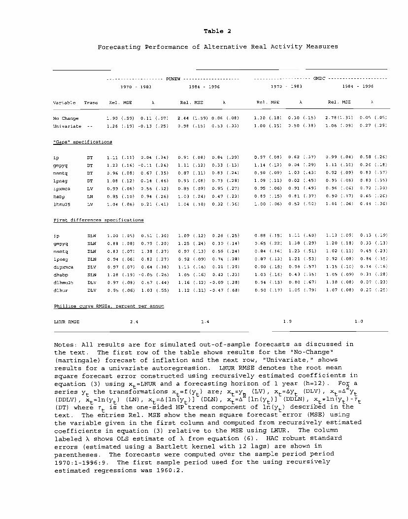
Table 2
Forecasting Performance of Alternative Real Activity Measures
p1970 - 1983
Variable Trans Rel. MOE A
uw1984 - 1996
Rel. MOE A Rel.
1970
MSE
GMDC
- 1983
A
1984
Eel. MOE
- 1996
No Change 1.90 (.59) 0.11 (.07) 2.44 (1.59) 0.06 (.08) 1.30 (.18) 0.30 (.15) 2.78(1.31) -0.05 (.05)
Univariate -- 1.26 (.19) -0.13 (.25) 0.98 (.15) 0.53 (.33) 1.00 (.15) 0.50 (.38) 1.06 (.09) 0.27 (.29)
'Gaps specifications
ip DT 1.11 (.11) 0.04 (.34) 0.91 (.08) 0.84 (.29) 0.97 (.08) 0.62 (.37) 0.99 (.04) 0.58 (.26)
gmpyq DT 1.23 (.16) -0.11 (.26) 1.11 (.12) 0.33 (.13) 1.14 (.12) 0.04 (.29) 1.11 (.10) 0.26 (.18)
msmtq DT 0.96 (.08) 0.67 (.35) 0.87 (.11) 0.83 (.24) 0.90 (.09) 1.03 (.43) 0.92 (.09) 0.83 (.37)
lpnag DT 1.08 (.12) 0.14 (.46) 0.93 (.08) 0.73 (.28) 1.09 (.11) 0.02 (.45) 0.93 (.08) 0.83 (.35)
ipxlsca LV 0.99 (.06) 0.56 (.32) 0.85 (.09) 0.95 (.27) 0.95 (.06) 0.91 (.49) 0.96 (.06) 0.72 (.30)
habp LN 0.85 (.10) 0.94 (.26) 1.03 (.24) 0.47 (.23) 0.89 (.15) 0.81 (.37) 0.90 (.17) 0.65 (.26)
lhmu2S LV 1.04 (.06) 0.21 (.41) 1.04 (.10) 0.32 (.36) 1.00 (.06) 0.52 (.50) 1.01 (.06) 0.44 (.36)
First differences specifications
ip DLN 1.00 (.05) 0.51 (.30) 1.09 (.12) 0.26 (.25) 0.88 (.15) 1.11 (.60) 1.13 (.09) 0.13 (.19)
gmpyq DLN 0.88 (.08) 0.79 (.20) 1.25 (.24) 0.30 (.14) 0.65 (.22) 1.38 (.29) 1.20 (.18) 0.33 (.13)
msmtq DLN 0.83 (.07) 1.38 (.27) 0.97 (.13) 0.55 (.24) 0.84 (.16) 1.23 (.51) 1.02 (.11) 0.45 (.23)
lpnag DLN 0.94 (.06) 0.82 (.27) 0.92 (.09) 0.74 (.28) 0.87 (.13) 1.21 (.53) 0.92 (.08) 0.84 (.35)
dipxmca DLV 0.97 (.07) 0.64 (.36) 1.13 (.16) 0.21 (.29) 0.90 (.15) 0.96 (.57) 1.15 (.10) 0.14 (.16)
dhsbp DLN 1.28 (.19) -0.05 (.26) 1.05 (.16) 0.42 (.23) 1.03 (.16) 0.43 (.35) 1.05 (.09) 0.31 (.28)
dlhmu25 DLV 0.97 (.08) 0.67 (.44) 1.16 (.12) -0.09 (.28) 0.94 (.15) 0.80 (.67) 1.10 (.08) 0.07 (.23)
dihur DLV 0.95 (.06) 1.03 (.55) 1.12 (.11) -0.47 (.68) 0.90 (.17) 1.05 (.79) 1.07 (.08) 0.20 (.25)
Phillips curve Rl'SEs, percent per annum
1.4 1.9 1.0LHUR RMSE 2.4
Notes: All results are for simulated out-of-sample forecasts as discussed inthe text. The first row of the table shows results for the lNochangeTl(martingale) forecast of inflation and the next row, "TJnivariate," showsresults for a univariate autoregression. LHUR RMSE denotes the root meansquare forecast error constructed using recursively estimated coefficients inequation (3) using xt=LHtJR and a forecasting horizon of 1 year (h=12) . Fo a
series y the transformations xt=f(yt) are; x=y (LV), xt=yt (DLV), x=(DDLV), x=ln(y) (LN), x=L[ln(y)] (DLN), x=E [ln(yt)] x=ln(y)-T(DT) where is the one-sided HP trend component of ln(yt) described in thetext. The entries Rel. MSE show the mean square forecast error (MSE) usingthe variable given in the first column and computed from recursively estimatedcoefficients in equation (3) relative to the MSE using LHTJR. The columnlabeled X shows OLS estimate of X from equation (6) . HAC robust standarderrors (estimated using a Bartlett kernel with 12 lags) are shown inparentheses. The forecasts were computed over the sample period period1970:1-1996:9. The first sample period used for the using recursivelyestimated regressions was 1960:2.

Table 3
Forecasting Performance of Various Economic Indicators
puww GMDC
1970 - 1983 1984 - 1996 1970 - 1983 1984 - 1996
Variable Trans Rel. MSE A Rel. MSE A Rel. MSE A Re1. MSE A
Univariate -- 1.26 (.19) -0.13 (.25) 0.98 (.15) 0.53 (.33) 1.00 (.15) 0.50 (.38) 106 (.09) 0.27 (.29)
Interest Rates
fyff DLV 1.34 (.33) 0.05 (.16) 1.02 (.15) 0.44 (.33) 1.07 (.20) 0.37 (.35) 1.06 (.08) 0.25 (.29)
fycp DLV 1.25 (.18) 0.06 (.17) 1.04 (.16) 0.42 (.33) 1.03 (.16) 0.42 (.38) 1.07 (.08) 0.23 (.30)
fygm3 DLV 1.27 (.24) 0.06 (.20) 1.01 (.15) 0.47 (.31) 1.09 (.19) 0.31 (.38) 1.06 (.08) 0.25 (.29)
fygm6 DLV 1.25 (.21) 0.03 (.22) 1.04 (.15) 0.42 (.31) 1.02 (.16) 0.46 (.43) 1.06 (.08) 0.24 (.29)
fygtl DLV 1.21 (.17) 0.08 (.22) 1.03 (.15) 0.42 (.32) 1.02 (.15) 0.45 (.40) 1.06 (.08) 0.25 (.30)
fygt5 DLV 1.24 (.18) -0.03 (.24) 1.13 (.24) 0.37 (.21) 1.01 (.16) 0.48 (.38) 1.06 (.09) 0.27 (.29)
fygtlo DLV 1.23 (.21) 0.19 (.25) 1.11 (.25) 0.41 (.19) 1.02 (.15) 0.45 (.36) 1.06 (.09) 0.26 (.29)
fyaaac DLV 1.26 (.22) 0.26 (.17) 1.26 (.39) 0.34 (.20) 1.14 (.19) 0.32 (.19) 1.07 (.10) 0.25 (.29)
fybaac DLV 1.12 (.18) 0.40 (.14) 1.23 (.38) 0.36 (.18) 1.15 (.18) 0.33 (.17) 1.08 (.12) 0.34 (.20)
fyfha DLV 1.31 (.24) 0.19 (.20) 1.26 (.29) 0.30 (.16) 1.02 (.16) 0.45 (.37) 1.07 (.09) 0.26 (.29)
sp_fyIf LV 1.21 (.18) 0.00 (.29) 1.11 (.18) 0.31 (.27) 1.04 (.19) 0.41 (.46) 1.17 (.11) 0.02 (.21)sp_fycp LV 1.17 (.15) 0.12 (.26) 1.09 (.21) 0.38 (.24) 0.99 (.14) 0.52 (.39) 1.11 (.13) 0.25 (.26)
spfygm6 LV 1.14 (.21) 0.37 (.17) 1.16 (.26) 0.34 (.20) 1.06 (.16) 0.43 (.18) 1.19 (.17) 0.15 (.23)
spfygtl LV 1.40 (.29) -0.13 (.18) 0.97 (.18) 0.55 (.29) 1.06 (.15) 0.38 (.28) 1.07 (.10) 0.28 (.30)
spfygt5 LV 1.08 (.12) 0.42 (.11) 1.62 (.73) 0.18 (.19) 1.25 (.21) 0.25 (.16) 1.44 (.41) 0.12 (.20)
spfygtlo LV 1.10 (.15) 0.39 (.15) 1.68 (.73) 0.14 (.19) 1.23 (.20) 0.24 (.17) 1.51 (.40) 0.05 (.20)
spfyaaac LV 1.10 (.15) 0.37 (.18) 1.54 (.45) 0.10 (.20) 1.21 (.21) 0.24 (.19) 1.39 (.28) 0.05 (.23)
sp_fybaac LV 1.18 (.21) 0.30 (.20) 1.32 (.26) 0.05 (.18) 1.29 (.26) 0.15 (.19) 1.12 (.07) 0.07 (.19)sp_fyfha LV 1.22 (.22) 0.27 (.19) 1.30 (.28) 0.22 (.18) 1.29 (.26) 0.16 (.18) 1.11 (.10) 0.18 (.25)
Nominal Money
fml DLN 1.25 (.19) 0.11 (.20) 1.08 (.26) 0.42 (.23) 1.06 (.17) 0.38 (.32) 1.05 (.10) 0.37 (.24)
fm2 DLN 1.29 (.19) -0.01 (.23) 0.97 (.13) 0.53 (.17) 1.05 (.16) 0.39 (.34) 0.98 (.08) 0.54 (.21)
fm3 DLN 1.27 (.20) -0.07 (.25) 1.00 (.12) 0.50 (.17) 1.03 (.15) 0.43 (.35) 1.01 (.08) 0.49 (.19)
fmJ. DUO 1.28 (.26) 0.05 (.26) 1.12 (.14) 0.35 (.14) 1.06 (.18) 0.38 (.35) 1.06 (.09) 0.37 (.19)
fmfba DUO 1.27 (.21) -0.03 (.26) 1.11 (.27) 0.33 (.35) 1.04 (.18) 0.43 (.35) 1.13 (.16) 0.12 (.36)fmbase DLN 1.36 (.23) -0.18 (.23) 1.05 (.19) 0.42 (.31) 1.11 (.18) 0.29 (.33) 1.08 (.11) 0.23 (.30)
fmrra DLN 1.28 (.18) -0.14 (.26) 0.99 (.17) 0.51 (.27) 1.00 (.16) 0.51 (.39) 1.06 (.10) 0.31 (.27)fmrxiba ]OLN 1.26 (.18) -0.11 (.26) 1.07 (.16) 0.37 (.27) 1.01 (.15) 0.47 (.38) 1.07 (.09) 0.24 (.28)
fmrnbc DLN 1.25 (.18) -0.12 (.25) 1.04 (.16) 0.43 (.29) 1.00 (.15) 0.49 (.39) 1.07 (.09) 0.24 (.28)
fml DDLN 1.26 (.18) -0.12 (.25) 0.98 (.16) 0.53 (.33) 1.00 (.15) 0.50 (.39) 1.06 (.09) 0.28 (.29)
fm2 DDLN 1.26 (.19) -0.15 (.25) 0.99 (.16) 0.53 (.32) 1.00 (.15) 0.50 (.39) 1.07 (.09) 0.26 (.29)
fm3 DDLN 1.26 (.19) -0.14 (.25) 0.98 (.15) 0.53 (.33) 1.00 (.16) 0.49 (.39) 1.06 (.09) 0.27 (.29)
fml DDLN 1.26 (.19) -0.13 (.25) 0.99 (.16) 0.53 (.33) 1.00 (.16) 0.50 (.39) 1.06 (.09) 0.27 (.30)
fmfba DDLN 1.25 (.18) -0.10 (.25) 0.99 (.16) 0.53 (.32) 0.99 (.16) 0.51 (.39) 1.06 (.09) 0.29 (.29)
fmbase DDLN 1.26 (.19) -0.13 (.25) 0.98 (.16) 0.53 (.32) 1.00 (.16) 0.50 (.39) 1.06 (.09) 0.28 (.29)fmrra DDLN 1.26 (.18) -0.12 (.25) 0.98 (.16) 0.54 (.32) 1.00 (.16) 0.51 (.39) 1.06 (.09) 0.30 (.29)
fmrnba DDLN 1.26 (.19) -0.14 (.25) 0.99 (.16) 0.53 (.33) 0.99 (.16) 0.51 (.39) 1.06 (.09) 0.27 (.29)fmrnbc DDLN 1.26 (.19) -0.14 (.25) 0.98 (.16) 0.54 (.33) 0.99 (.16) 0.52 (.39) 1.06 (.09) 0.27 (.30)

Table 3 (Continued)
PUNEW GMDC
1970 - 1983 1984 - 1996 1970 - 1983 1984 - 1996
Variable Trans Rel. MSE X Rel. F4SE X Rel. MSE X Rel. MSE A
Exchange Rates
exrus DLN 1.33 (.36) 0.24 (.13) 1.94 ( 1.18) 0.19 (.1 1.32 (.37) 0.24 (.16) 1.66 (.69) 0.12 (.21)8)
exrger DLN 1.32 (.22) -0.12 (.24) 1.38 (.54) 0.24 (.24) 0.99 (.12) 0.52 (.20) 1.62 (.60) 0.05 (.23)
exrsw DLN 1.32 (.22) -0.07 (.22> 1.31 (.50) 0.26 (.27) 1.62 (.71) -0.12 (.21) 1.39 (.39) 0.03 (.28)
exrjan DLN 1.42 (.33) 0.30 (.08) 1.49 (.50) 0.30 (.15) 1.49 (.34) 0.26 (.09) 1.14 (.16) 0.19 (.26)
exruk DLN 1.27 (.19) -0.15 (.25) 1.01 (.17) 0.47 (.32) 1.04 (.13) 0.39 (.36) 1.08 (.10) 0.22 (.30)
exrcan DLN 1.28 (.18) -0.20 (.25) 0.98 (.16) 0.54 (.33) 1.0]. (.15) 0.48 (.38) 1.06 (.09) 0.31 (.28)
Prices and Wages
pmcp LV 1.25 (.18) -0.16 (.31) 1.08 (.20) 0.39 (.26) 1.06 (.14) 0.33 (.39) 1.09 (.09) 0.20 (.28)
pwfsa DDLN 1.26 (.18) -0.11 (.25) 0.97 (.15) 0.56 (.32) 1.00 (.15) 0.51 (.38) 1.05 (.09) 0.31 (.28)
pwfcsa DDLN 1.25 (.18) -0.11 (.25) 0.98 (.15) 0.55 (.32) 0.99 (.16) 0.53 (.38) 1.05 (.09) 0.32 (.28)
pwimsa DDLN 1.26 (.19> -0.12 (.25) 0.98 (.15> 0.54 (.32) 1.00 (.16) 0.50 (.39) 1.06 (.09) 0.28 (.29)
pwcmsa DDLN 1.26 (.18> -0.12 (.25) 0.98 (.15) 0.54 (.32) 1.04 (.18) 0.41 (.36) 1.06 (.09) 0.29 (.29)
psm99q DDLN 1.37 (.23> -0.24 (.22) 1.27 (.28) 0.24 (.21) 1.02 (.15) 0.46 (.37) 1.06 (.09) 0.28 (.29)
punew DDLN 1.26 (.19) -0.13 (.25) 0.98 (.15) 0.53 (.33) 1.01 (.15) 0.48 (.38) 1.06 (.09) 0.29 (.29)
pu83 DDL.N 1.26 (.19) -0.13 (.25) 0.99 (.16) 0.51 (.32) 1.00 (.16) 0.49 (.38) 1.07 (.09) 0.26 (.29)
pu84 DDLN 1.26 (.19) -0.13 (.25) 0.98 (.15> 0.54 (.32) 1.00 (.15) 0.50 (.39) 1.06 (.09) 0.30 (.27)
puc DDLN 1.26 (.19) -0.13 (.25) 0.98 (.15) 0.54 (.32) 1.00 (.15) 0.49 (.39) 1.05 (.09) 0.31 (.29)
pucd DDLN 1.24 (.18) -0.08 (.26> 0.99 (.16) 0.52 (.32) 1.00 (.15) 0.49 (.38) 1.06 (.09) 0.29 (.29)
pus DDLN 1.26 (.19) -0.13 (.25) 0.99 (.16) 0.53 (.33) 1.00 (.16) 0.51 (.39) 1.06 (.09) 0.27 (.29)
puxf DDLN 1.26 (.18) -0.12 (.25) 0.98 (.15) 0.54 (.32) 1.00 (.15) 0.50 (.39) 1.06 (.09) 0.28 (.29)
puxhs DDLN 1.26 (.19) -0.13 (.25) 0.98 (.15) 0.54 (.33) 1.00 (.15) 0.49 (.38) 1.06 (.09) 0.27 (.29)
puxm DDLN 1.25 (.18> -0.12 (.26) 0.98 (.15> 0.54 (.32) 1.00 (.15) 0.50 (.39) 1.06 (.09) 0.30 (.29)
gmdc DI3LN 1.26 (.19) -0.12 (.24) 0.99 (.15> 0.53 (.33) 1.00 (.15) 0.50 (.38) 1.06 (.09) 0.27 (.29)
gmdcd DDLN 1.26 (.19) -0.12 (.25) 0.99 (.16) 0.53 (.33) 1.00 (.15) 0.49 (.38) 1.06 (.09) 0.28 (.29)
gmdcn DDLN 1.27 (.19) -0.12 (.24) 0.98 (.15) 0.54 (.32) 1.00 (.15) 0.49 (.38> 1.04 (.08) 0.35 (.27)
gnidca DDLN 1.26 (.19) -0.14 (.25> 0.98 (.16) 0.53 (.32) 0.99 (.16> 0.51 (.39) 1.05 (.09) 0.33 (.29)
lehcc DDLN 1.26 (.19) -0.13 (.25) 0.99 (.15) 0.53 (.32) 1.00 (.15) 0.49 (.38) 1.06 (.09) 0.28 (.29)
lehm DDLN 1.26 (.19) -0.13 (.25) 0.98 (.15) 0.53 (.33) 1.00 (.15) 0.50 (.38) 1.06 (.09) 0.27 (.29)
Output
ipp DLN 0.97 (.06) 0.67 (.30) 1.14 (.15) 0.19 (.24) 0.85 (.16) 1.13 (.53) 1.15 (.11) 0.20 (.1'?)
ipf DLN 1.03 (.08) 0.34 (.36> 1.07 (.12) 0.33 (.23) 0.90 (.15) 0.96 (.57) 1.17 (.12) 0.12 (.19)
ipc DLN 1.10 (.12) 0.20 (.28) 1.00 (.10) 0.50 (.19) 0.92 (.16) 0.76 (.49) 1.13 (.09) 0.22 (.17)
ipcd DLN 1.21 (.16) -0.10 (.31) 1.10 (.12) 0.31 (.22) 1.02 (.15) 0.45 (.41) 1.12 (.09) 0.14 (.23)
ipcn DLN 1.16 (.15) 0.06 (.26) 0.97 (.15) 0.53 (.17) 0.99 (.15) 0.52 (.45) 1.09 (.13) 0.37 (.18)
(pc DLN 1.00 (.07) 0,48 (.42) 1.11 (.12) 0.27 (.18) 0.87 (.18) 1.05 (.60) 1.17 (.11) -0.02 .20)
ipi DUO 0.84 (.07) 1.05 (.20) 1.12 (.12) 0.33 (.14) 0.84 (.17) 0.96 (.42) 1.11 (.10) 0.31 (.16)
1pm DUO 1.10 (.10) 0.09 (.39) 1.04 (.12) 0.40 (.26) 0.98 (.14) 0.61 (.62) 1.14 (.09) 0.00 (.20)
ipod DLN 1.12 (.12) 0.07 (.39> 1.03 (.09) 0.42 (.23) 1.00 (.15) 0.48 (.62) 1.13 (.09) 0.10 (.18)
ipand DL.N 1.15 (.09) -0.03 (.27) 1.03 (.12) 0.45 (.17) 1.01 (.15) 0.48 (.52) 1.08 (.07) 0.31 (.17)
ipmfg DLN 0.96 (.05) 0.76 (.36) 1.11 (.13) 0.21 (.25) 0.87 (.15) 1.17 (.61) 1.11 (.08) 0.19 (.18)
ipd DUO 0.99 (.07) 0.56 (.39) 1.14 (.15) 0.18 (.26) 0.91 (.15) 0.97 (.66) 1.18 (.10) 0.05 (.16)
ipn DUO 1.08 (.10) 0.21 (.29) 1.07 (.11) 0.41 (.13) 0.91 (.16> 0.80 (.50) 1.08 (.08) 0.35 (.14)
ipmin DUO 1.25 (.18) -0.08 (.25> 1.00 (.16) 0.51 (.33) 1.01 (.15) 0.48 (.37) 1.06 (.09) 0.28 (.29)
iput DUO 1.28 (.17) -0.23 (.24> 1.00 (.15) 0.50 (.25) 1.03 (.15) 0.41 (.39) 1.05 (.09) 0.33 (.25)
pmi LV 0.74 (.08) 1.73 (.29) 0.96 (.15) 0.56 (.24) 0.73 (.21) 1.51 (.46) 0.99 (.13) 0.53 (.28)
pmp LV 0.89 (.07) 0.89 (.26) 1.01 (.13) 0.49 (.21) 0.80 (.20) 1.18 (.50) 1.15 (.15) 0.29 (.19)
gmyxpq DUO 0.84 (.07> 0.86 (.23) 1.42 (.38) 0.08 (.17) 0.73 (.18) 1.20 (.27) 1.27 (.22) 0.25 .13)
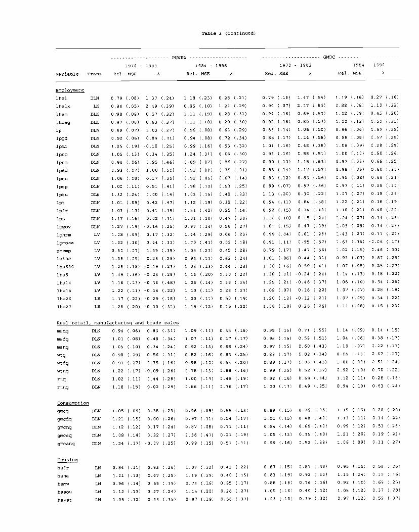
Table 3 (Continued)
PUNEW GMDC
1970 - 1983 1984 - 1996 1970 - 1983 1984 - 1996
Variable Trans Rel. MSE A Rel. MSE A Rel. MSE A Rel. MSE A
Employment
lhel DLN 0.79 (.08) 1.37 (.24) 1.18 (.23) 0.28 (.21) 0.79 (.18) 1.47 (.54) 1.19 (.16) 0.27 (.16)
iheix LN 0.84 (.05) 2.49 (.39) 0.85 (.10) 1.21 (.29) 0.90 (.07) 2.17 (.85) 0.88 (.08) 1.10 (.32)
lhem DLN 0.98 (.08) 0.57 (.32) 1.11 (.19) 0.28 (.31) 0.94 (.16) 0.69 (.53) 1.02 (.09) 0.45 (.20)
lhnag DLN 0.97 (.08) 0.63 (.37) 1.11 (.18) 0.29 (.30) 0.92 (.16) 0.80 (.57) 1.00 (.12) 0.50 (.21)
ip DLN 0.89 (.07) 1.03 (.27) 0.96 (.08) 0.63 (.29) 0.88 (.14) 1.06 (.50) 0.96 (.06) 0.69 (.29)
lpgd DLN 0.92 (.06) 0.89 (.31) 0.94 (.08) 0.72 (.34) 0.85 (.17) 1.14 (.58) 0.98 (.08) 0.57 (.28)
lpmi DLN 1.25 (.19) -0.10 (.25) 0.99 (.16) 0.53 (.32) 1.01 (.16) 0.48 (.38) 1.06 (.09) 0.28 (.29)
lpcc DLN 1.05 (.13) 0.34 (.35) 1.24 (.31) 0.06 (.30) 0.98 (.16) 0.58 (.51) 1.00 (.10) 0.50 (.26)
ipem DLN 0.94 (.06) 0.95 (.46) 0.89 (.07) 0.86 (.27) 0.90 (.13) 1.15 (.63) 0.97 (.05) 0.66 (.25)
iped DLN 0.93 (.07) 1.00 (.50) 0.92 (.08) 0.75 (.31) 0.88 (.14) 1.17 (.57) 0.98 (.06) 0.60 (.30)
lpen DLN 1.06 (.08) 0.17 (.35) 0.92 (.06) 0.67 (.14) 0.93 (.12) 0.83 (.56) 0.95 (.08) 0.64 (.21)
lpsp DLN 1.00 (.11) 0.51 (.41) 0.98 (.13) 0.53 (.25) 0.99 (.07) 0.57 (.36) 0.97 (.11) 0.58 (.30)
iptu DLN 1.32 (.24) 0.00 (.14) 1.03 (.15) 0.42 (.33) 1.13 (.20) 0.30 (.22) 1.07 (.07) 0.19 (.28)
ipt DLN 1.01 (.09) 0.42 (.47) 1.12 (.19) 0.32 (.22) 0.94 (.11) 0.84 (.58) 1.22 (.21) 0.18 (.19)
lpfr DLN 1.03 (.13) 0.41 (.35) 1.51 (.42) 0.25 (.14) 0.92 (.15) 0.74 (.43) 1.10 (.21) 0.40 (.20)
ips DLN 1.17 (.16) 0.02 (.31) 1.01 (.10) 0.47 (.30) 1.10 (.10) 0.15 (.24) 1.04 (.07) 0.34 (.28)
lpgov DLN 1.27 (.19) -0.16 (.25) 0.97 (.14) 0.56 (.27) 1.01 (.15) 0.47 (.39) 1.05 (.08) 0.34 (.23)
lphrm LV 1.08 (.09) 0.17 (.32) 1.44 (.29) 0.06 (.23) 0.99 (.04) 0.61 (.28) 1.43 (.23) -0.11 (.21)
lpmosa LV 1.02 (.10) 0.44 (.33) 1.70 (.41) 0.02 (.18) 0.91 (.11) 0.95 (.57) 1.63 (.36) -0.06 (.17)
pmemp LV 0.80 (.07) 1.39 (.35) 1.04 (.23) 0.45 (.28) 0.79 (.17) 1.47 (.56) 1.02 (.15) 0.46 (.30)
luinc LV 1.08 (.09) 0.26 (.28) 0.94 (.11) 0.62 (.24) 1.01 (.06) 0.44 (.31) 0.93 (.07) 0.87 (.29)
1hu680 LV 1.28 (.18) -0.19 (.23) 1.03 (.13) 0.44 (.28) 1.00 (.16) 0.50 (.41) 1.07 (.08) 0.25 (.27)
lhuS LV 1.49 (.36) -0.23 (.28) 1.14 (.20) 0.30 (.22) 1.38 (.31) -0.24 (.24) 1.14 (.13) 0.18 (.22)
1hu14 LV 1.18 (.13) -0.36 (.48) 1.06 (.14) 0.38 (.26) 1.25 (.21) -0.46 (.37) 1.06 (.10) 0.34 (.26)
lhulS LV 1.22 (.11) -0.34 (.22) 1.10 (.11) 0.28 (.23) 1.08 (.07) 0.16 (.22) 1.07 (.07) 0.28 (.18)
1hu26 LV 1.37 (.22) -0.29 (.18) 1.00 (.11) 0.50 (.19) 1.20 (.13) -0.12 (.21) 1.07 (.09) 0.34 (.22)
].hu27 LV 1.28 (.20) -0.30 (.31) 1.15 (.12) 0.15 (.22) 1.08 (.10) 0.26 (.26) 1.11 (.08) 0.15 (.23)
Real retail, manufacturing and trade sales
1.09 (.11) 0.35 (.16) 0.95 (.15) 0.71 (.55) 1.14 (.09) 0.14 (.15)msmq DLN 0.94 (.06) 0.83 (.31)
msdq DLN 1.01 (.08) 0.48 (.34) 1.07 (.11) 0.37 (.17) 0.98 (.15) 0.58 (.51) 1.04 (.06) 0.38 (.17)
msnq DLN 1.05 (.10) 0.34 (.24) 0.92 (.13) 0.65 (.24) 0.97 (.15) 0.60 (.43) 1.10 (.07) 0.22 (.17)
wtq DIN 0.98 (.09) 0.56 (.31) 0.82 (.16) 0.83 (.25) 0.88 (.17) 0.82 (.34) 0.86 (.13) 0.87 (.27)
wtdg DLN 0.91 (.07) 0.75 (.16) 0.98 (.10) 0.54 (.20) 0.89 (.17) 0.83 (.43) 1.00 (.08) 0.51 (.24)
wtnq DLN 1.22 (.17) -0.09 (.26) 0.78 (.13) 0.88 (.16) 0.99 (.15) 0.52 (.37) 0.92 (.10) 0.70 (.22)
rtq DLN 1.02 (.11) 0.44 (.28) 1.00 (.13) 0.49 (.19) 0.92 (.16) 0.69 (.34) 1.12 (.11) 0.28 (.18)
rtnq DLN 1.18 (.15) 0.02 (.29) 0.86 (.11) 0.76 (.17) 1.00 (.13) 0.49 (.35) 0.94 (.10) 0.63 (.24)
Consumption
gmcq DLN 1.05 (.09) 0.38 (.23) 0.96 (.09) 0.55 (.13) 0.89 (.15) 0.76 (.35) 1.15 (.15) 0.28 (.20)
gmcdq DLN 1.21 (.15) 0.00 (.26) 0.97 (.11) 0.54 (.17) 1.01 (.15) 0.48 (.40) 1.13 (.11) 0.14 (.22)
gmcnq DLN 1.12 (.12) 0.17 (.24) 0.87 (.08) 0.71 (.11) 0.94 (.14) 0.69 (.40) 0.99 (.12) 0.53 (.26)
gmcsq DLN 1.08 (.14) 0.32 (.27) 1.36 (.41) 0.21 (.19) 1.05 (.13) 0.35 (.40) 1.21 (.20) 0.19 (.23)
gmcanq DLN 1.24 (.17) -0.07 (.25) 0.99 (.15) 0.51 (.31) 0.99 (.16) 0.52 (.38) 1.06 (.09) 0.31 (.27)
Housing
hsfr LN 0.84 (.11) 0.93 (.26) 1.07 (.22) 0.43 (.22) 0.87 (.15) 0.87 (.38) 0.95 (.16) 0.58 (.25)
hsne LN 1.01 (.13) 0.47 (.25) 1.19 (.29) 0.40 (.15) 0.83 (.19) 0.92 (.43) 1.15 (.24) 0.39 (.16)
hsmw LN 0.96 (.14) 0.55 (.19) 0.73 (.16) 0.85 (.17) 0.88 (.18) 0.76 (.36) 0.92 (.10) 0.69 (.25)
hssou LN 1.12 (.13) 0.27 (.24) 1.15 (.20) 0.26 (.27) 1.05 (.16) 0.40 (.32) 1.05 (.12) 0.37 (.28)
hswst LN 1.05 (.12) 0.33 (.35) 0.97 (.19) 0.56 (.37) 1.03 (.10) 0.39 (.32) 0.97 (.12) 0.59 (.37)

Notes: See the notes to Table 2.
Table 3 (Continued)
PUNEW GMDC
1970 - 1983 1984 - 1996 1970 - 1983 1984 - 1996
Variable Trans Rel. WSE A Rel. MSE A Rel. MSE A Rel. WSE A
hsbp IN 0.85 (.10) 0.94 (.26) 1.03 (.24) 0.47 (.23) 0.89 (.15) 0.81 (.37> 0.90 (.17) 0.65 (.26)
dhsbp DLN 1.28 (.19) -0.05 (.26) 1.05 (.16) 0.42 (.23) 1.03 (.16) 0.43 (.35) 1.05 (.09) 0.31 (.28)
hsbr IN 0.85 (.10) 0.94 (.26) 1.03 (.24) 0.47 (.23) 0.89 (.15) 0.81 (.37) 0.90 (.17) 0.65 L26,
hmob LN 1.33 (.18) -0.24 (.29) 1.10 (.19) 0.33 (.28) 1.07 (.16) 0.34 (.36) 1.04(06) 0.34 (.25)
condo9 LN 1.23 (.21) 0.03 (.29) 1.25 (.20) 0.16 (.16) 1.05 (.21) 0.40 (.39) 1.02 (.09) 0.42 (.30)
Inventories and Orders
(.16) -0.18 (.26) 1.06 (.12) 0.37 (.22) 0.97 (.13> 0.58 (.43) 1.09 (.07) 0.22 (.21)ivmtq DLN 1.22
ivmfgq DIN 1.27 (.19) -0.17 (.25) 0.99 (.13) 0.51 (.29) 1.06 (.11) 0.31 (.31) 1.02 (.07) 0.42 (.25)
ivmfdq DLN 1.23 (.17) -0.10 (.26) 0.98 (.12) 0.54 (.28) 1.03 (.11) 0.41 (.34) 1.03 (.07) 0.40 (.22)
ivmfnq DLN 1.26 (.20) -0.05 (.24) 1.01 (.17) 0.48 (.32) 1.01 (.15) 0.48 (.35) 1.09 (.11) 0.21 (.28)
ivwrq DIN 1.24 (.18> -0.11 (.24) 0.98 (.15) 0.54 (.30) 1.00 (.15) 0.49 (.39) 1.05 (.08) 0.34 (.27)
ivrrq DLN 1.22 (.17) -0.11 (.28) 1.14 (.17) 0.20 (.28) 0.99 (.16) 0.52 (.42) 1.11 (.09) 0.14 (24)
ivsrq DLV 1.03 (.09) 0.40 (.26) 1.07 (.11) 0.41 (.15) 0.99 (.16) 0.52 (.39) 1.07 (.08) 0.33 (.17)
ivsrmq DLV 1.11 (.14) 0.22 (.30) 1.17 (.16) 0.26 (.18) 0.98 (.16) 0.55 (.39) 1.17 (.12) 0.04 (.23)
ivsrwq DLV 1.10 (.10) 0.29 (.25) 0.91 (.09) 0.65 (.14) 0.98 (.18) 0.55 (.37) 1.02 (.08) 0.46 (.21)
ivsrrq DLV 1.26 (.18) -0.12 (.25) 0.98 (.15) 0.54 (.31) 1.01 (.13) 0.48 (.33) 1.05 (.08) 0.33 (.27)
pmnv LV 1.02 (.10) 0.43 (.36) 0.90 (.11) 0.66 (.19) 0.87 (.17) 1.05 (.57) 0.94 (.09) 0.64 (.21)
pmno LV 0.85 (.06) 1.30 (.32> 1.01 (.14) 0.49 (.19) 0.80 (.19) 1.40 (.57) 1.08 (.16) 0.39 (.21)
mocmq DLN 1.05 (.10) 0.34 (.30> 1.07 (.09) 0.38 (.14) 0.94 (.15> 0.68 (.46) 1.13 (.08) 0.17 (.15)
mdoq DIN 0.91 (.06) 0.92 (.21) 1.15 (.17> 0.27 (.16> 0.95 (.15> 0.72 (.54) 1.08 (.07) 0.30 (.13)
msondq DIN 1.08 (.13) 0.27 (.31) 1.28 (.27) 0.03 (.26> 0.98 (.15) 0.56 (.44) 1.14 (.11) 0.11 (.20)
mpconq DLN 1.08 (.13) 0.26 (.32) 1.32 (.31) 0.02 (.25> 1.00 (.15) 0.51 (.40) 1.13 (.10) 0.04 (.27)
Stock Prices
fsricom DIN 1.24 (.18) -0.03 (.23) 1.14 (.22) 0.31 (.25) 1.02 (.16) 0.45 (.35) 1.07 (.09) 0.27 (.27)
fspcom DLN 1.24 (.18) -0.04 (.24) 1.17 (.23) 0.27 (.24) 1.02 (.16) 0.46 (.36) 1.07 (.09) 0.27 (.26)
fspin DLN 1.24 (.18) -0.03 (.24) 1.14 (.22) 0.31 (.25) 1.02 (.16) 0.45 (.35) 1.07 (.09) 0.27 (.26)
fspcap DIN 1.23 (.17) 0.00 (.23) 1.23 (.25) 0.22 (.22) 1.04 (.16) 0.42 (.35) 1.08 (.09) 0.24 (.25)
fsput DLN 1.26 (.19) -0.12 (.25) 0.99 (.16) 0.52 (.33) 1.02 (.15) 0.46 (.37) 1.06 (.09) 0.27 (.29)
fsdxp LV 1.55 (.68) 0.09 (.25) 1.04 (.19) 0.44 (.26) 1.20 (.41) 0.32 (.31) 1.16 (.13) 0.16 (.23)
fspxe LV 1.33 (.22) -0.08 (.25) 1.18 (.24> 0.33 (.19) 1.03 (.17) 0.42 (.38) 1.28 (.26) 0.12 (.19)
Other Variables
fm2dq DLN 1.22 (.17) 0.13 (.24> 0.91 (.14) 0.58 (.13) 0.99 (.15) 0.52 (.32) 0.89 .11) 068 (.17)
fclnq DLN 1.30 (.20) -0.13 (.22) 0.99 (.14) 0.51 (.33) 1.11 (.11> 0.21 (.26) 1.06 (.07) 0.32 (.20)
fclbrnc LV 1.36 (.25) -0.13 (.26) 2.79 ( 3.96) 0.07 (.1 1.21 (.29) 0.15 (.35) 1.16 (.16) 0.15 (.22)1)hhsntn LV 1.52 (.33) -0.47 (.27) 0.91 (.08) 0.74 (.20> 1.27 (.18) -0.10 (.21) 0.97 (.07) 0.64 (.29)
pmdel LV 1.02 (.09> 0.45 (.25) 0.89 (.11) 0.76 (.27) 0.91 (.14) 0.78 (.41) 0.88 (.10) 0.77 (.23)
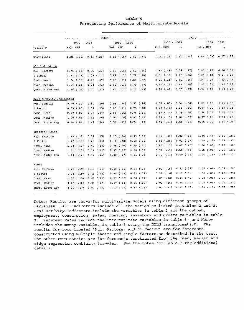
Table 4Forecasting Performance of Multivariate Models
1970 -Variable Rel. MSE
1983
X
PUNEW
1984 -Rel. MSE
1996X Rel.
1970 - 1983
MSE A
GMDC
Rel.
1984 -MSE
1996
A
univariate 1.26 (.19) -0.13 (.25) 0.98 (.15) 0.53 (.33) 1.00 (.15) 0.50 (.38) 1.06 (.09) 0.27 (.29)
All Indicators
Mu).. Factors 0.79 (.11) 0.95 (.21) 0.97 (.16) 0.53 (.16) 0.97 (.09) 0.59 (.27) 0.86 (.17) 0.66 (.17)
1 Factor 0.77 (.09) 1.08 (.17) 0.83 (.13) 0.78 (.20) 0.81 (.16) 1.06 (.36) 0.84 (.12) 0.91 (.26)
Comb. Mean 1.04 (.09) 0.29 (.39) 0.88 (.09) 0.87 (.27) 0.91 (.14) 0.89 (.55) 0.97 (.05) 0.63 (.26)
Comb. Median 1.14 (.13) 0.03 (.31) 0.92 (.11) 0.70 (.29) 0.95 (.15) 0.64 (.46) 1.02 (.07) 0.40 (.28)
Comb. Ridge Reg. 0.86 (.06) 1.20 (.22) 0.87 (.17) 0.73 (.29) 0.90 (.09) 1.15 (.39) 0.94 (.10) 0.63 (.23)
Real Activity Indicators
1.31 (.20) 0.99 (.16) 0.51 (.18) 0.88 (.09) 0.97 (.28) 0.81 (.16) 0.76 (.19)Mul. Factors 0.70 (.10)
1 Factor 0.69 (.09) 1.82 (.25) 0.88 (.11) 0.75 (.18) 0.77 (.19) 1.21 (.46) 0.87 (.12) 0.86 (.25)
Comb. Mean 0.97 (.07) 0.72 (.47) 0.88 (.06) 0.96 (.19) 0.87 (.14) 1.29 (.66) 0.94 (.06) 0.78 (.26)
Comb. Median 1.00 (.08) 0.53 (.46) 0.90 (.06) 0.87 (.19) 0.89 (.15) 1.04 (.65) 0.97 (.05) 0.64 (.25)
Comb. Ridge Reg. 0.84 (.06) 1.47 (.34> 0.90 (.11) 0.74 (.25) 0.84 (.13) 1.55 (.50> 0.95 (.10) 0.61 (.21)
Interest Rates
Mul. Factors 1.37 (.35) 0.21 (.15) 1.25 (.34) 0.33 (.17) 1.39 (.38) 0.02 (.18) 1.39 (.48) -0.00 (.26)
1 Factor 1.27 (.18) 0.23 (.15) 1.40 (.42) 0.18 (.20) 1.41 (.29) -0.01 (.17) 1.19 (.13> 0.01 (.23)
Comb. Mean 1.03 (.11> 0.42 (.28) 0.96 (.15) 0.59 (.31) 0.96 (.13) 0.62 (.40) 1.06 (.08) 0.28 (.30)
Comb. Median 1.11 (.13> 0.21 (.30) 0.95 (.15) 0.60 (.32) 0.97 (.15) 0.58 (.43) 1.05 (.08) 0.29 (.29)
Comb. Ridge Reg. 1.04 (.12) 0.42 (.24) 1.00 (.17) 0.51 (.31) 1.00 (.13) 0.49 (.34) 1.14 (.11) 0.09 (.23)
2flMul. Factors 1.26 (.19) -0.13 (.25) 0.98 (.16) 0.53 (.33) 0.99 (.16> 0.52 (.39) 1.06 (.09) 0.29 (.29)
1 Factor 1.26 (.19) -0.13 (.25) 0.98 (.16) 0.53 (.33) 0.99 (.16) 0.52 (.39) 1.06 (.09) 0.29 (.29)
Comb. Mean 1.25 (.19) -0.05 (.26) 0.97 (.15) 0.56 (.27) 1.03 (.16) 0.44 (.37) 1.03 (.08) 0.39 (.26)
Comb. Median 1.25 (.18) -0.08 (.27> 0.97 (.14) 0.56 (.27) 1.02 (.16) 0.46 (.37) 1.04 (.09) 0.37 (.27)
Comb. Ridge Reg. 1.22 (.17) 0.02 (.26> 1.02 (.16) 0.47 (.25) 1.00 (.17) 0.51 (.36) 1.14 (.12) 0.17 (.22)
Notes: Results are shown for multivariate models using different groups ofvariables. All Indicators include all the variables listed in tables 2 and 3.Real Activity Indicators include the variables in table 2 and the output,employment, consumption, sales, housing, inventory and orders variables in table3. Interest Rates include the interest rate variables in table 3, and Moneyincludes the money variables in table 3 using the DDLN transformation. Theresults for rows labeled "Mul. FactorsT and tl] Factor" are for forecastsconstructed using multiple factor and single factors as described in the text.The other rows entries are for forecasts constructed from the mean, median andridge regression combining formular. See the notes for Table 2 for additionaldetails.

Table 5Forecasting Performance Relative to Real Activity Single Factor Model
Univariate
1 hur
1.83 (.50) -0.22 (.14)
1.46 (.19) -0.82 (.25)
1.12 (.30) 0.37 (.25)
1.14 (.15) 0.25 (.18)
1.29 (.23) 0.20 (.17)
1.29 (.32) -0.21 (.46)
1.23 (.25) 0.09 (.26)
1.16 (.16) 0.14 (.25)
description of the table entriesconstructed from the single
activity factor model. The results shown under descriptor Activity FactorCombined With are for forecasts constructed using a recursive OLS combinationof the single activity forecast with single factor forecasts from the modelslisted in the first column.
PUNEW GMDC
1970 - 1983 1984 - 1996 1970 - 1983 1984 - 1996
Variable Rel. MSE A Rel. MSE A Rel. MSE A Rel. MSE A
All Indicators
Mul. Factors 1.15 (.13) 0.00 (.36) 1.11 (.12) 0.22 (.31) 1.25 (.26) -0.13 (.40) 1.00 (.12) 0.51 (.23)
1 Factor 1.12 (.13) 0.04 (.44) 0.94 (.09) 1.03 (.74) 1.05 (.13) 0.30 (.46) 0.98 (.05) 0.79 (.55)
Comb. Mean 1.52 (.29) -0.29 (.20) 1.01 (.18) 0.48 (.32) 1.18 (.18) 0.21 (.23) 1.13 (.16) 0.09 (.34)
Comb. Median 1.66 (.38) -0.26 (.16) 1.05 (.23) 0.43 (.27) 1.23 (.20) 0.21 (.19) 1.18 (.21) 0.10 (.28)
Comb. Ridge Reg. 1.25 (.13) -0.53 (.30) 1.00 (.16) 0.51 (.50) 1.17 (.20) -0.03 (.47) 1.09 (.08) 0.11 (.31)
Real Activity Indicators
(.08) 0.35 (.51) 1.13 (.12) -0.05 (.42) 1.14 (.20) -0.10 (.61) 0.94 (.10) 0.67 (.28)Mul. Factors 1.02
Comb. Mean 1.41 (.21) -0.40 (.22) 1.00 (.12) 0.50 (.36) 1.12 (.14) 0.22 (.28) 1.09 (.11) 0.02 (.39)
Comb. Median 1.45 (.24) -0.41 (.20) 1.03 (.13) 0.43 (.33) 1.15 (.16) 0.20 (.25) 1.13 (.12) -0.09 (.35)
Comb. Ridge Reg. 1.23 (.11) -0.50 (.23) 1.02 (.07) 0.32 (.54) 1.08 (.12) 0.23 (.36) 1.10 (.06) 0.06 (.28,
Interest Rates
Mul. Factors 1.99 (.84) -0.02 (.13) 1.42 (.49) 0.22 (.19) 1.79 (.79) -0.03 (.14) 1.61 (.71) -0.08 (.23)
1 Factor 1.85 (.51) -0.04 (.16) 1.60 (.59) 0.16 (.17) 1.83 (.59) -0.11 (.16) 1.37 (.28) -0.12 (.23)
Comb. Mean 1.50 (.32) -0.06 (.22) 1.09 (.26) 0.41 (.23) 1.24 (.22) 0.18 (.23) 1.22 (.22) 0.06 (.26)
Comb. Median 1.62 (.37) -0.15 (.20) 1.08 (.27) 0.41 (.24) 1.26 (.22) 0.20 (.20) 1.22 (.24) 0.08 (.27)
Comb. Ridge Reg. 1.51 (.33) -0.01 (.20) 1.14 (.27) 0.36 (.23) 1.30 (.22) 0.15 (.20) 1.32 (.25) -0.04 (.22)
yMul. Factors 1.84 (.50) -0.23 (.15) 1.12 (.30) 0.37 (.25) 1.28 (.22) 0.21 (.16) 1.22 (.24) 0.10 (.26)
1 FactOr 1.84 (.50) -0.23 (.15) 1.12 (.30) 0.37 (.25) 1.28 (.22) 0.21 (.16) 1.22 (.24) 0.10 (.26)Comb. Mean 1.82 (.49) -0.20 (.15) 1.11 (.27) 0.38 (.25) 1.32 (.24) 0.18 (.17) 1.19 (.22) 0.12 (.28)Comb. Median 1.82 (.48) -0.22 (.16) 1.10 (.28) 0.39 (.24) 1.31 (.23) 0.19 (.17) 1.20 (.23) 0.13 (.27)
Comb. Ridge Reg. 1.78 (.45) -0.16 (.15) 1.17 (.30) 0.34 (.23) 1.29 (.18) 0.22 (.14) 1.32 (.27) 0.02 (.22)
Activity Factor Combined With:
-0.63
-0.10(18)
0.21
0.13
(.38)
(.12)
(.10)
0.99
1.01
1.09
1.10
(.01)
(.02)
(.05)
(.06)
1.46
-0.01
-1.35
-1.48
(1.42)
(.98)
(.87)
(.89)
1.08
1.08
1.04
1.11
(.11)
(.11)
(.06)
(.11)
0.05
0.26
0.31
0.28
(.50)
(.28)
(.28)
(.20)
1.07
1.11
1.071.04
(.05)
(.05)
(.05)
(.04)
-0.21
-0.22
-0.28
0.04
(.35)
(.24)
(.45)
(.42)
1.19 (.08)
1.30 (.24)
1.21 (.15)
1.44 (.29)
All Indicators
Interest Rates
Money
mt. Rates, Money
Activity Factor
RMSE (% per annum) 2.0 1.3 1.7
Notes: See the notes to tables 2 and 4 for aThe benchmark forecast used in this table is
1.0

Table 6Forecasting Performance of 1(0) Models of Inflation
Relative to Real Activity Single Factor Model
All Indicators
Mul. Factors
1 Factor
1.06 (.13) 0.35 (.28)1.18 (.17) -0.13 (.47)
1.30 (.31) 0.15 (.30)
0.92 (.10) 1.20 (.78)
1.36 (.39) 0.15 (.23)
1.19 (.20) -0.17 (.49)1.24 (.28) 0.26 (.23)0.94 (.05) 1.48 (.69)
Activity Factor
RNSE (% per annum) 2.1
Notes: See the notes to tables 2 and 4 for a description of the tableentries. The benchmark forecast used in this table is constructed from thesingle activity factor model. All of the specifications except the entrylabeled "Table 5 Benchmark" are based on equation (12)
PUNEW GMDC
1970 - 1983 1984 - 1996 1970 - 1983 1984 - 1996
Variable Rel. MSE A Rel. MSE A Rel. MSE A Rel. MSE A
Table 5 Benchmark 0.89 (.07) 1.72 (.63) 1.08 (.08) -0.54 (.61) 0.97 (.07) 0.66 (.46) 1.04 (.07) 0.22 (.49)
lhur 1.52 (.40) -0.22 (.36) 1.19 (.16) 0.16 (.18) 1.65 (.71) -0.42 (.41) 1.12 (.13) 0.12 (.32)
Univariate 1.63 (.35) -0.19 (.18) 1.15 (.28) 0.35 (.23) 1.41 (.30) -0.05 (.20) 1.17 (.18) 0.12 (.28)
Real Activity Indicators
Mul. Factors 1.01 (.19) 0.49 (.46) 1.16 (.21) 0.06 (.48) 1.22 (.34) 0.06 (.46) 1.02 (.11) 0.45 (.29)
ipxmca 1.33 (.17) -0.35 (.28) 0.95 (.16) 0.61 (.37) 1.29 (.30) -0.24 (.46) 1.07 (.14) 0.25 (.42)
hsbp 1.54 (.39) -0.45 (.38) 1.11 (.15) 0.25 (.24) 1.59 (.65) -0.23 (.34) 1.03 (.14) 0.44 (.32)lhmu25 1.32 (.15) -0.52 (.27) 1.16 (.15) 0.17 (.26) 1.32 (.18) -0.63 (.31) 1.17 (.09) -0.06 .26)
msmtq 1.15 (.12) 0.04 (.31) 1.16 (.31) 0.21 (.47) 1.08 (.12) 0.22 (.36) 1.00 (.15) 0.50 .53)
Interest Rates
Mul. Factors 3.30(3.00) -0.09 (.10) 1.39 (.48) 0.27 (.18) 3.14(3.45) -0.02 (.11) 1.39 (.38) 0.04 (.23)
iFactor 3.10(3.15) -0.18 (.07) 1.14 (.26) 0.36 (.21) 2.64)2.56) 0.01 (.13) 1.18 (.18) 0.13 (.26)
fygm3 2.32(1.28) -0.14 (.12) 1.21 (.27) 0.28 (.22) 2.12(1.15) 0.04 (.14) 1.20 (.18) 0.07 (.25)
ygt1 2.80(2.56) -0.13 (.10) 1.19 (.28) 0.32 (.21) 2.23(1.43) 0.06 (.13) 1.19 (.18) 0.11 (.26)
fygm3-CI 2.11 (.92) -0.07 (.13) 1.30 (.40) 0.15 (.23) 1.88 (.87) 0.06 (.16) 1.26 (.26) -0.11 (.31)
fygtl-CX 2.17(1.09) -0.06 (.13) 1.30 (.38> 0.12 (.22) 2.01 (1.17) 0.10 (.13) 1.27 (.26) -0.14 (.31)
Money
Mul. Factors 1.60 (.35) 0.01 (.15) 1.60 (.58) 0.05 (.23) 1.32 (.24) 0.03 (.24) 1.43 (.30) -0.02 (.20)1 Factor 1.65 (.34) -0.08 (.20) 1.26 (.35) 0.31 (.23) 1.41 (.23) -0.04 (.18) 1.12 (.18) 0.32 (.26)
fm2 1.92 (.47) -0.23 (.16) 0.99 (.22) 0.51 (.26) 1.53 (.33) -0.13 (.19) 1.01 (.14) 0.47 (.32)
fmbase 1.55 (.30> -0.01 (.20) 1.69 (.70) 0.15 (.19> 1.40 (.22) 0.01 (.17) 1.35 (.28) -0.03 (.25)
Prices
pmcp 1.29 (.16) -0.36 (.28) 1.25 (.35) 0.27 (.27) 1.22 (.27) -0.09 (.44) 1.28 (.30) 0.07 (.36)
psrn99q 0.97 (.11) 0.55 (.21) 1.28 (.28) 0.28 (.20) 1.01 (.08) 0.48 (.17) 1.42 (.28) 0.00 (.21)
exrus 1.65 (.38) 0.10 (.10) 2.40(1.86) 0.17 (.13) 1.51 (.40) 0.14 (.12) 1.94 (.98) 0.07 (.16)
1.2 1.8 1.0

C)
U
C)
U—
Figure 1Annual Inflation
(N
a
0Cc
0
LO
0•0
0
(N
0
00 1960 1965 1970 1975 1980 1985 1990 1995 2000
Year

C)U)
C0aU,C)
C)(flO:3-,a°
a00
C)(I)C0a(I)C)
a)U)
:3aE
Figure 2Estimated Impulse Responses for Different Sample Periods
A. PUNEW
'I I
Horizon
B. GMDC
Horizon

FigureReal Activity
3
Inicators
(N-
C
0-
I I
U)
C0
0>
n-d
I'I.
I
Activity Factor
II
/
— — Unemp. Rote (Inverted)
I I I I
1960 1965 1970 1975 1980 1985 1990 1995 2000
Year

Q)
U
U)
0
0
0a
1000i 1965 1970
Figure 4Annual CR1 Inflation and Forecasts Made 12 Months Earher
03
d
b
0Cd
10
R0
I I I
I, I
.1
CPI Inflation— — unemp. Rote Forecast
Activity Factor Forecast
I I I
1975 1980 1985 1990
Year
1995 2000