forecasting models - timothy s. wood

Forecasting Models

Timothy S. Wood, Student Western Kentucky University

February 26, 2014 [email protected]

Module 3 Forecasting Models

Executive Summary Forecasting is an essential part of every business that is being run all over the world today. To remain successful in today’s times it is essential for businesses to look to the future so as that they can have a plan in place to be ready for an ever changing world. A plan needs to be made to show future possible trends in what a business may experience.

In this report it will show several different businesses and how they all can have a forecast to have an estimate on what might happen in the future.

1 | P a g e

Module 3


Contents Executive Summary ........................................................ 1

Contents ......................................................................... 2

Problem 1 ....................................................................... 3

Problem 1 ....................................................................... 4

Problem 1 ....................................................................... 5

Problem 1 ....................................................................... 6

Problem 1 ....................................................................... 7

Problem 2 ....................................................................... 8

Problem 2 ..................................................................... 10

Problem 2 ..................................................................... 11

Problem 3 ..................................................................... 12

Problem 3 ..................................................................... 13

Problem 3 ..................................................................... 14

Problem 3 ..................................................................... 15

Conclusion .................................................................... 16

Appendix ....................................................................... 17

2 | P a g e

Module 3


Problem 1 In this forecast we are looking into National Scan, Inc. and looking into their selling of radio tags. We will walk through the forecasting model and try to show how they can have several different forecasting techniques and then they can decide on which one they should trust more to base their projections on the future on.

Table 1.1 lists the actual number of units that National Scan, Inc. has sold for the past 7 months.

Table 1.1 Number of Actual Number of Units That Were Sold Over the Past 7 Months at National Scan, Inc...

Table 1.2 shows the linear trend forecasting technique be used to project the future for the month of September.

Table 1.2 Linear Trend Forecasting Technique to Forecast the Number of Units to be Sold for the Month of September.

3 | P a g e

Module 3


Problem 1 a) For Table 1.2 it was made with Excel computing the formula for a linear trend

and then plugged into the months and then shows a projection for the month of September based on that formula. In projection it forecast that for the month of September National Scan, Inc. will sell 20,857 units.

Chart 1.1 is the trendline chart that was used to come up with the formula for the linear trend equation that was used to get the figures for Table 1.2

Chart 1.1 is the Chart that was Used to come up with the Formula for the Linear Trend Forecast in Table 1.2

a) In this chart the actual sales numbers were used and Excel computed theformula in Chart 1.1 of y = 500x + 16857 to come up with all the figures in Table1.2.

4 | P a g e

Module 3


Problem 1 Table 1.3 shows the naïve forecasting technique being used to forecast the number of units that will be sold for September.

Table 1.3 Uses the Naïve Forecasting Technique to Forecast the Number of Units to be Sold for September.

a) For Table 1.3 it was based on the naïve forecasting technique and this forecast basically says what was sold last month will be sold the next month. With this in mind it forecasted that 20,000 units would be sold for September as this is what was actually sold for the prior month of August.

Table 1.4 shows 5 month moving average being used to project the number of units that will be sold in September.

Table 1.4 Uses a 5 Month Moving Average to Forecast the Number of Units to be Sold for the Month of September.

5 | P a g e

Module 3


Problem 1 a) The 5 month moving average forecast in Table 1.3 shows that National Scan, Inc.

will sell 19,000 units for the month of September.

Table 1.5 uses and exponential smoothing forecasting technique that uses a smoothing constant of Alpha = .2 to forecast the number of units sales for the month of September.

Table 1.5 Uses the Exponential Smoothing Technique to Forecast the Number of Units to be Sold for the Month of September.

a) The exponential smoothing forecasting technique in Table 1.5 shows that National Scan, Inc. will sell 20,320 units for the month of September. The formula for this is equal to the previous month sales + Alpha (the smoothing constant of .2) times (actual month sales projection – previous month sales).

6 | P a g e

Module 3


Problem 1 Table 1.6 shows weighted average forecasting technique in forecasting the month of September.

Table 1.6 Uses the Weighted Average Forecasting Technique to Forecast the Number of Units to be Sold for September.

a) The weighted average forecasting technique in Table 1.6 shows that NationalScan, Inc. will sell 20,400 units for the month of September. This technique basesa decimal weighted formula and uses that to come up with an estimate.

b) The formula for this technique is equal to (.1 times June actual sales) + (.3 times July actual sales) + (.6 times August actual sales) and uses the result of this as the number of units that will be sold in September.

Recommendation

All 5 forecasting techniques came up with number somewhere around 20,000 units with the exception of the 5 month moving average which came in at 19,000 units. With all the forecasting techniques in mind it seems that somewhere around the 20,000 units’ sales mark should be good bases for the sales forecast for September. With this in mind National Scan, Inc. could use the 20,000 units to be sold number in for the forecast of what they should be able to sell in the month of September.

7 | P a g e

Module 3


Problem 2 In this problem we are looking into a generic electrical contractors weekly records to come with a forecast for a future week to show the number of requests forecast for that week. This could be used by that electrical contractor to base the number of requests for that week and give the contractor some ideal as to how many requests they will have in that week.

Table 2.1 shows the actual number of requests for a 5 week period for the electrical contractor.

Table 2.1 shows the actual number of request that the electrical contractor had during a given 5 week period.

8 | P a g e

Module 3


Chart 2.1 shows the number of requests that the electrical contractor had over a 5 week period.

Chart 2.1 Shows the Number of Requests that the Electrical Contractor had over a 5 Week Period.

a) This chart can be used to help visualize the number of requests that theelectrical contractor is having over a 5 week period. This can be used to come upwith several forecasts to help the contractor plan for the upcoming week’snumber of requests.

9 | P a g e

Module 3


Problem 2 Table 2.2 uses the naïve forecasting technique to come up with a table to show the projected number of requests for that electrical contractors’ sixth week.

Table 2.2 Uses the Naïve Forecasting Technique to come up with a Forecast for Week number six.

a) The naïve forecasting technique is being used to come up the number of requests the electrical contractor will have in the sixth week. The forecast for the sixth week is 22 requests, based on using this technique.

Table 2.3 uses the 4 week moving average to forecast the number of requests for the sixth week.

Table 2.3 Uses a 4 Week moving Average to Come up With the Forecast for the Sixth Weeks’ Number of Requests.

a) In the 4 week moving average forecast the number of requests forecast for thesixth week is 20 requests.

10 | P a g e

Module 3


Problem 2 Table 2.4 uses the exponential smoothing forecasting technique to forecast the number of requests that the electrical contractor will have in the sixth week.

Table 2.4 Uses the Exponential Smoothing Forecasting Technique to Forecast the Number of Requests that the Electrical Contractor will have in the Sixth week.

a) The exponential smoothing forecasting technique is being used to come up witha forecast of 15.4 requests for the sixth week.

b) This technique uses the formula of being equal to the previous weeks requests +the Alpha (.3 smoothing constant) times (actual week requests – previous weekrequests).

Recommendation

In looking at these three forecasts the exponential smoothing forecast comes up with a forecast of 15.4 requests, the naïve comes up with 22 requests, and the 4 week moving average comes up with 20 requests. This leaves electrical contractors with a forecast of going with the somewhere around 20 requests to 15.4 requests for the week as a good range to base how many request that they will have in week sixth.

11 | P a g e

Module 3


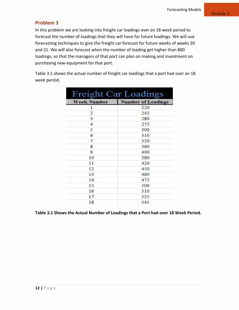
Problem 3 In this problem we are looking into freight car loadings over an 18 week period to forecast the number of loadings that they will have for future loadings. We will use forecasting techniques to give the freight car forecast for future weeks of weeks 20 and 21. We will also forecast when the number of loading get higher than 800 loadings, so that the managers of that port can plan on making and investment on purchasing new equipment for that port.

Table 3.1 shows the actual number of freight car loadings that a port had over an 18 week period.

Table 3.1 Shows the Actual Number of Loadings that a Port had over 18 Week Period.

12 | P a g e

Module 3


Problem 3 Chart 3.1 is being used to come up with a linear trendline and then we will use the equation that is derived from that trendline to make a linear trend forecast.

Chart 3.1 shows the Linear Trendline for the Data that came from the Freight Car loadings Actual Number of Loadings over an 18 Week period.

a) This linear trendline has been used to come up with a formula to be used toproject the future forecast for the number of freight car loadings that this portwill have for future weeks of 20 and 21.

b) The linear trendline came up with an equation of y = 18.996x + 208.48. This iswhere x is the number of the week times the 18.996 figure then 208.48 is addedto it to make the forecast for each week after that.

13 | P a g e

Module 3


Problem 3 Table 3.2 uses the equation from the linear trendline Chart 3.1 to make a forecast for the future weeks of 20 and 21 and also to show when the number of loadings goes over the number of 800.

Table 3.2 Shows the Forecast of a Linear Trend equation to Forecast the Number of Future Loadings for the Given Port.

a) Using the linear trend equation to forecast the future for weeks 20 and 21, aforecast for week 20 is 588 and week 21 is 607 freight car loadings for this port.The forecast for week 20 and 21 was based on the equation of 18.996 times theweek number then adding 208.48 to them.

b) In looking ahead to estimate when this ports’ freight car loadings will exceed 800loadings, it is forecasted that this will happen in week number 32. In weeknumber 32 it is forecasted with the linear trend equation that this port will have816 freight car loadings.

14 | P a g e

Module 3


Problem 3

Recommendation

In looking at the freight car loadings for this port we can see that using the linear trend equation has given a good forecast for the week of 20 having 588 loadings and week of 21 having 607 loadings. This can be used by this port to forecast these numbers for the future freight car loadings that will be experienced. It also gives this port a good future forecast for this port as to when the freight car loading will rise above the 800 mark. The forecast for when the loadings will exceed the 800 mark is forecasted to be on week number 32 and this forecast is that the port will have 816 loadings during this week.

15 | P a g e

Module 3


Conclusion

This report covers three different situations to give forecasts of what the future might bring for each of the different situations. In the forecast it was given using a variety of different forecasting techniques so as to give each situation several different forecasts to be analyzed for basing a sound forecast on.

For Problem number one it was for National Scan, Inc. and this forecast was based on using five different forecasting techniques. This National Scan forecast used the naïve, five month moving average, exponential smoothing, and weighted average forecasting techniques. In looking at all five forecasts, four of the forecasts it was forecasted that 20,000-20,857 units would be sold for the month of September.

For Problem number 2 it was for a generic electrical contractor and this forecast was based on three different forecasting techniques. The electrical contractors forecast involved the naïve, 4 week moving average and the exponential smoothing forecasting techniques. In looking into the electrical contractors forecast for requests for the sixth week two of the forecast came in closer in projecting 20-22 requests for the sixth week. The other forecast came in at 15.4 requests for the sixth week and with all three being used it can be forecasted that the electrical contractor will have a range of 15.4-22 requests for the sixth week.

For problem number 3 it dealt with freight car loadings for a generic port. This forecast was done with using a linear trend equation that was found from making a chart and inserting a trendline into the charts data. This trendline came up with an equation that was used to forecast the future weeks of 20 and 21. This forecast gave the port the forecasted freight car loadings for week 20 to be 588 and week 21 to be 607. It also was forecasted that the port would exceed 800 loadings in the week number 32. In week number 32 it was forecasted that this port will have 816 freight car loadings. This can be used by the managers of this port to invest on new equipment on week number 32.

Finally all of the forecasts can be used to base a sound forecast for them. The forecasts can then be used to make plans on what needs the businesses will need to handle the forecasts for these future timeframes.

16 | P a g e

Module 3


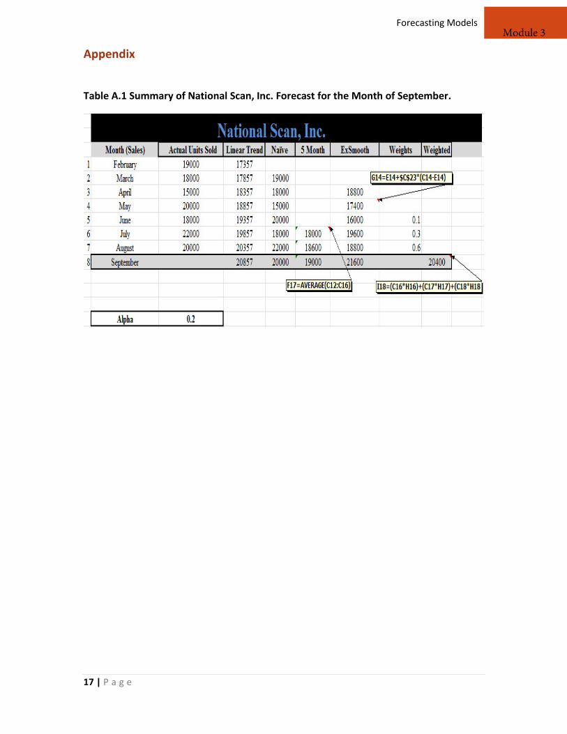
Appendix

Table A.1 Summary of National Scan, Inc. Forecast for the Month of September.

17 | P a g e

Module 3

forecasting models - timothy s. wood

Documents