forecasting nigerian stock market returns using … nigerian stock... · cbn journal of applied...

CBN Journal of Applied Statistics Vol. 5 No.2 (December, 2014) 25

Forecasting Nigerian Stock Market Returns using ARIMA and

Artificial Neural Network Models

1Godknows M. Isenah and Olusanya E. Olubusoye

The study reports empirical evidence that artificial neural network based

models are applicable to forecasting of stock market returns. The Nigerian

stock market logarithmic returns time series was tested for the presence of

memory using the Hurst coefficient before the models were trained. The test

showed that the logarithmic returns process is not a random walk and that the

Nigerian stock market is not efficient. Two artificial neural network based

models were developed in the study. These networks are

and whose out-of-sample forecast performance was

compared with a baseline model. The results obtained in the

study showed that artificial neural network based models are capable of

mimicking closely the log-returns as compared to the based model.

The out-of-sample evaluations of the trained models were based on the

, , and the directional change metric respectively.

Based on these metrics, it was found that the artificial neural network based

models outperformed the based model in forecasting future

developments of the returns process. Another result of the study shows that

instead of using extensive market data, simple technical indicators can be

used as predictors for forecasting future values of the stock market returns

given that the returns has memory of its past.

Keywords: Artificial neural networks, Long memory, Random walk,

Forecasting, Training, Stock Market Returns, Technical analysis indicator,

ARIMA.

JEL Classification: E44, G17

1.0 Introduction

Artificial neural networks are one of the most popular tools for forecasting

financial and economic time series. They are universal and highly flexible

function approximators for pattern recognition and classification, [Beresteanu

(2003); Chan et al. (2009)]. An artificial neural network based model requires

1 Department of Statistics, University of Ibadan, Nigeria E-mail:

[email protected],[email protected]

mailto:[email protected]


26 Forecasting Nigerian Stock Market Returns using ARIMA and Artificial

Neural Network Models Isenah & Olubusoye

no prior assumptions on the behaviour and functional form of the related

variables, but can still capture the underlying dynamics and nonlinear

relationships that exist amongst the variables. This paper proposes artificial

neural network based models for forecasting the Nigerian Stock Exchange All-

Share-Index logarithmic returns, and comparing the out-of-sample forecast

performance of the networks with a baseline model.

In stock market predictions, many methods for technical analysis and

forecasting have been developed and are being used, [see Pring (1985)]. In

technical forecasting, technical indices (in the form of rolling means, rolling

standard deviations/or variances, lagged values etc.) are usually computed

from a time series and are used to forecast future changes in the levels of the

series. Several artificial neural network based models have been developed for

stock market forecasting. Some of these models are applied to forecasting the

future rates of changes of stock prices, [see Kimoto et al (1990)], and some

are applied to recognizing certain patterns in stock prices that are

characteristics of the future price changes, [Kamojo and Tanigawa (1990)].

The performance of artificial neural networks has been extensively compared

to that of various parametric statistical methods within the areas of prediction

and classification [Ripley (1996)]. In particular, some literature on time series

forecasting using artificial neural networks has been generated, though, with

mixed results. Some of the articles reviewed on the performance of artificial

neural networks at the time of this study are Lepedes and Farber (1987), Tang

et al. (1991), Shada(1994) and Stern (1996). These articles show that neural

network models outperform conventional parametric models especially for

time series with little or no stochastic component. An interesting result by

Tang et al. (1991) is that the relative performance of an artificial neural

network model is influenced by the memory of the time series when compared

with the Box-Jenkins ARIMA models.

In Nigeria, Akinwale et al. (2009) used regression neural network with back-

propagation algorithm to analyze and predict translated and un-translated

Nigerian stock market prices (NSMP). Their study compared forecast

performance of the neural networks with translated and un-translated NSMP

as inputs, and this revealed that the network with translated NMSP inputs

outperformed the network with un-translated NSMP inputs. In terms of

prediction accuracy measures, the translated NSMP network predicted


accurately 11.3% of the stock prices as compared to 2.7% prediction accuracy

of the un-translated NSMP network model.

Similarly, from the ARIMA scheme’s perspective of forecasting the Nigerian

stock market returns, Ojo and Olatayo (2009) studied the estimation and

performance of subset autoregressive integrated moving average (ARIMA)

models. They estimated parameters for ARIMA and subset ARIMA processes

using numerical iterative schemes of Newton-Raphson and the Marquardt-

Levenberg algorithms. The performance of the models and their residual

variance were examined using AIC and BIC. The result of their study showed

that the SARIMA model outperformed the ARIMA model with smaller

residual variance. On the other hand, Emenike (2010) studied the NSE market

returns series using monthly data of the All-Share-Index for the period

January 1985 through December 2008. In his study, an ARIMA (1,1,1) model

was selected as a tentative model for predicting index points and growth rates.

The results revealed that the global meltdown destroyed the correlation

structure existing between the NSE All-Share-Index and its past values.

Agwuegbo et al. (2010) also studied the daily returns process of the Nigerian

Stock Market using Discrete Time Markov Chains , and martingales.

Their study provided evidence that the daily stock returns process follows a

random walk, but that the stock market itself is not efficient even in weak

form.

Several other studies that have used ARIMA schemes for analysis and

forecasting of stock market prices/or returns in Africa include Simons and

Laryea (2004), Rahman and Hossain (2006), and Al-Shiab (2006) among

others. These studies did not test whether or not the stock price/or returns

processes are fractal in nature. This we intend to determine for the Nigerian

stock market before we proceed with further analysis.

For our study, we will apply the Feed-forward multilayer perceptron (MLP)

neural network models with a single hidden layer. The architecture of the log-

returns prediction system for the Nigerian stock market consists of a pre-

processing unit, a MLP neural network and a post-processing unit. The pre-

processing unit scales each of the inputs (the predictors) to have zero mean

and standard deviation of 1, before they are passed into the network for

processing. In a similar fashion, the response variable (log-return) is scaled to

fall within the interval of the activation functions of the neural network. The

output/or signal produced by the neural network is then passed to the post-



processing unit which converts the networks output/or signal to the predicted

stock market returns.

The Box and Jenkins (1976) ARIMA method of forecasting is different from

most optimization based methods. This technique does not assume any

particular pattern in the historical data of the time series to be forecasted. It

uses iterative procedures to identify a tentative model from a general class of

models. The chosen model is then checked for adequacy and if found to be

inadequate, the modeling process is repeated all over again until a satisfactory

model is found.

The rest of the study is as follows: Section 2 discusses the Methodology,

Random Walk and Efficient Market Hypothesis, Tools for detection of

memory in time series, Statistical concepts and Training of artificial neural

networks. Section 3 discusses the proposed models and data analysis. Section

4 gives results and discussions, while Section 5 ends with summary and

conclusion.

2.0 Methodology

2.1 The random walk and efficient market hypotheses

A school of thought in the theory of financial econometrics that is widely

accepted by financial economists is the Efficient Market Hypothesis .

They believe generally that financial markets are very efficient in reflecting

information about individual securities traded in the markets and about the

market as a whole. The states, according to Ongorn (2009) that prices of

securities traded, for example: stocks, bonds, or properties reflects all known

information and therefore are unbiased in the sense that they reflect the

collective beliefs of all investors about the future prospects. Under the ,

information is quickly and efficiently incorporated into asset prices at any

point in time, so that the price history cannot be used to predict future price

movements of the assets. In general, under the , an asset price, say stocks,

denoted by already incorporates all relevant information, and the only

reason for the prices to change between time and time will be due to

shocks. The therefore postulates that the assets price process follow a

random walk. The random walk model without drift parameter is expressed

as:


where is a white noise process. When is not a white noise

process, the price series is said to have memory which violates the ,

[Shiriaev, (1999)]. According to Fama (1965; 1995), a stock market where

successive price changes in individual securities are independent, is by

definition a random walk. Stock prices following a random walk imply that

the price changes are independent of one another as the gains and losses

[Kendal, (1953)]. The independence of the random walk or the is valid

as long as the time series of the price changes of the securities does not have

memory. In this study, our objective is to forecast the monthly logarithmic

returns of the using artificial neural network based models with technical

analysis indicators of the returns as inputs. This objective can only be

achieved if the log-returns process has memory. And to test for the presence

of memory in the returns series, we employed the fractional difference

parameter of a fractal time series; the Hurst (1951) coefficient ; and

the sample autocorrelation and partial autocorrelation functions ) and

respectively.

2.2 Tools for detection of memory in stock market returns time series

The Hurst coefficient , is a measure of the bias in fractionally integrated

time series. This coefficient could be used to test financial time series for the

presence of memory. The presence of memory in a time series indicates the

possibility of predicting the future values using its history. The rescaled range,

analysis which was proposed by Hurst (1951), and later refined by

Mandelbrot and Ness (1968) and Mandelbrot (1975; 1982), is able to

distinguish a random series from a fractionally integrated series, irrespective

of the distribution of the underlying process. The statistic is the range of

partial sums of deviations of a time series from its mean, rescaled by its

standard deviation. Specifically, let denote a stationary time series, then the

statistic is defined as:

[

∑

∑

]

where

∑

is the sample mean and *

∑

+

is the

sample standard deviation. When there is absence of long memory in a



stationary time series, the statistic converges to a random variable ,

where denotes the length of the time series. However, when the stationary

time series has long memory, Mandelbrot (1975) showed that the

statistic converges to a random variable at , where is the Hurst

coefficient, [see also Zivot and Wang (2003) for more details].

The Hurst coefficient is computed using the expression:

It describes three distinct categories of time series. These categories are:(i)

describe uncorrelated noise processes, whether they are Gaussian or

not; (ii) describe ergodic processes with frequent reversals and

high volatility, and(iii) describe reinforcing processes that are

characterized by long memory.The Hurst coefficient is related to the

fractional differencing parameter , of a fractionally integrated time series.

The relationship is given by:

According to Hosking (1981; 1996) and Mills (2007), for values of

,

the series is stationary and has long memory. For values of

, the

time series is anti-persistent, while for values of

, the series is

stationary and ergodic. Therefore, the Hurst coefficient and the fractional

difference parameter, can be used interchangeably for testing for the

presence of long memory in a stationary time series.

The monthly NSE All-Share-Index logarithmic returns are defined as:

[

] [ ]

The application of the memory tests just discussed on the log-returns series

give the results reported in Table 1. From these results, we conclude that the

monthly log-returns do not follow a random walk and neither is the Nigerian

Stock market efficient; this confirming one of the results provided by


Agwuegbo et al (2010). Figures 1 through 3 (see Appendix) show the time

plots of the monthly NSE All-Share-Index and the monthly logarithmic

returns; sample and ; the histogram and quantile-quantile plot of

the log-returns. The graphs show that the returns process is stationary, but its

distribution is leptokurtic and skewed to the left with long tails. While the

plots of sample and further confirm the results of the memory test

above by showing small but significant spikes in the correlograms.

Table 1: Sample descriptive statistics of NSE log returns and memory test

results

2.3 Statistical concepts

The MultiLayer Perceptron neural networks describe mapping of input

variables onto the output variable . For the feed-forward

multilayer perceptron neural network with a single hidden layer and one

output variable, , is a function of the vector of input variables

. This relationship can be expressed using an MLP neural network model of

the form:

∑ ( ∑

)

where we define

( ∑

) (

)

is the vector of hidden layer nodes of the network;

is a function of the hidden layer nodes; denotes the number of nodes in the

hidden layer; is an activation function, and denotes the transpose of a

matrix. The parameter vector:

311 0.01738 0.00383 0.0686 2.05104 0.609996 0.109996

Standard

deviation of

log returns

Series

length (N)

Mean of

log returns

Rescaled

range

statistic

Hurst

coefficient

Fractional

difference

parameter

Variance of

log returns



contains all the weights of the neural network.

Artificial neural networks are known to possess the properties of universal

approximators, hence, it is possible to construct nonparametric estimators for

regression functions, [see Hornik et al (1989), Beresteanu (2003) and Franke

et al.(2004) for more details]. Given the regression time series model:

The response function, can be approximated by fitting a neural

network model to the predictor variables: and the response

variable . The parameters of the network can be estimated using the

nonlinear least squares estimator obtained by minimizing:

∑ ( )

∑ ∑ ( )

where denotes the fitted neural network model.

2.4 Estimation/or training of neural networks

The least squares criterion given by Equation is obviously a nonlinear

function of . In this study, the iterative scheme will be

applied for the minimization of . The iterative scheme is a local

gradient-based search, in which the first and second order derivatives of

with respect to the weight vector , and continuous updating of the

initial conditions of , by the derivatives until some stopping criteria are met.

Given the initial weight vector , we obtain a second-order Taylor series

expansion of , given as:

where

is the gradient of evaluated at and

is the

Hessian of evaluated at . The approximating sum of squares function

will have a stationary point when its gradient is zero, that is:


and this stationary point will be a minimum if is positive definite. If is

positive definite, then the Newton-Raphson step is:

The generic approach to the minimization of is theback-propagation.

The back-propagation algorithm is a two-pass filter, [Friedman et al. (2008)].

This can be computed by a forward and backward sweep over the network,

keeping track of only quantities local to each unit of the network. To create

the filter, the partial derivatives of (8) with respect to and are calculated,

which are respectively given by:

[

]

And

∑ [

]

The gradient descent update at the iteration using these derivatives

has the form:

∑

and

∑

where is the learning rate. Rewriting (13) and (14) as:

and



The quantities and are errors from the current model at the output and

hidden layer units respectively. These errors satisfy ∑ ,

which is known as back-propagation, [Friedman et al.(2008)].

3.0 Proposed artificial neural network based models and data analysis

3.1 The proposed models

The proposed artificial neural network based models to be trained in the study

are the multilayer perceptron feed-forward neural networks with one

hidden and oneoutput layers and without skip connections. The neural

network’s architecture is of the form:

And inputs nodes function:

∑

Activation or hidden nodes function:

( )

Output node function:

( ) ∑

Following the approach of Yao and Tan (2000) and Erik (2002), the neural

network’s architecture is denoted as: , where denotes the input

layer size, the hidden layer size and the output layer size respectively.

3.2 Data segmentation, input selection and processing

The log-returns time series is segmented into training and test data sets

respectively. The training data set comprises of data points from January 1985


through December 2009, while the test data set comprises of data points from

January, 2010 through December, 2010.

The inputs selected for the networks are technical indices. These indices

are:(i) Rolling means denoted as: One-month , three-month , six-

month and twelve-month moving averages.(ii) Lagged values

of the log-returns denoted as: one-period lagged values , two-period

lagged values and three-period lagged values .

Since the activation function chosen (i.e. the logistic function) has its output

values in the interval [0, 1], the output variable was first scaled to have values

in this interval using the transformation:

The de-scaled log-returns fitted by the network are then obtained using the

expression:

[ ]

Similarly, the input variables (technical indices) were normalized to have

mean zero and standard deviation of one using:

3.3 Evaluation of neural networks

In- sample-evaluations criteria

The structures of the fitted neural networks at the training stages are compared

using the following order determination criteria to decide the best networks.

Akaike information criterion defined by:

[

∑

]

Hannan-Quinn information criterion defined by:



[

∑

]

[ ]

Bayesian information criterion defined by:

[

∑

]

where is the number of estimated parameters.

Out-sample-evaluations criteria

Comparisons of the predictive powers of the trained models are determined by

the use of the following metrics.

Root mean square error defined by:

*∑

+

Mean absolute error defined by:

∑ | |

Normalized mean square error defined by:

∑

∑

∑

Directional change statistic defined by:

∑

where {

and is the number of

observations in the test data set and { }.

4.0 Results and Discussions

This section presents discussions and the results obtained in the process of

analyzing the data using S-PLUS 6.1 Professional Edition. The following

parameters were held constant at their respective values throughout the


training process. Maximum number of iteration per fitted neural network: 200,

Tours: 300, Range (random range from uniform distribution for weight vector

selection):[-0.7, +0.7], Absolute tolerance: , Relative tolerance: , and

Output type: Linear. The penalty parameters were varied at the values 0.001,

0.01, 0.05 and 0.10 for each trained neural network model.

4.1 Technical Analysis and Forecasting using Rolling Means as Inputs

to the Networks

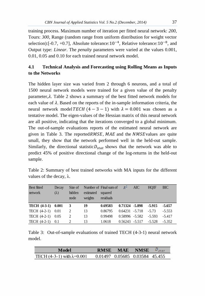
The hidden layer size was varied from 2 through 6 neurons, and a total of

1500 neural network models were trained for a given value of the penalty

parameter, . Table 2 shows a summary of the best fitted network models for

each value of . Based on the reports of the in-sample information criteria, the

neural network model with was chosen as a

tentative model. The eigen-values of the Hessian matrix of this neural network

are all positive, indicating that the iterations converged to a global minimum.

The out-of-sample evaluations reports of the estimated neural network are

given in Table 3. The reported , and the values are quite

small, they show that the network performed well in the held-out sample.

Similarly, the directional statistic shows that the network was able to

predict 45% of positive directional change of the log-returns in the held-out

sample.

Table 2: Summary of best trained networks with MA inputs for the different

values of the decay, λ.

Table 3: Out-of-sample evaluations of trained TECH (4-3-1) neural network

model.

Best fitted

network

Decay

(λ)

Size of

hidden

node

Number of

estimated

weights

Final sum of

squared

residuals

AIC HQIF BIC

TECH (4-3-1) 0.001 3 19 0.69583 0.71324 -5.898 -5.915 -5.657

TECH (4-2-1) 0.01 2 13 0.86795 0.64231 -5.718 -5.73 -5.553

TECH (4-2-1) 0.05 2 13 0.99498 0.58996 -5.582 -5.593 -5.417

TECH (4-2-1) 0.1 2 13 1.0618 0.56243 -5.517 -5.528 -5.352

Model RMSE MAE NMSE

TECH (4-3-1) with λ=0.001 0.01497 0.05685 0.03584 45.455



4.2 Technical analysis and Forecasting using Autoregressive inputs to

the Networks

The order of the autoregressive inputs to the nonlinear

autoregression, neural networks weredetermined using

maximum likelihood estimation with . The best order of the

autoregressive inputs to the network is 3 [see Table 4]. Again, the size of the

hidden layer of the network was varied between 2 and 6 inclusive for the

given values of the decay parameter. The summary of the results obtained in

the training process are presented in Tables 5. From this table, network model

TECH (3-3-1) with λ=0.001, was chosen as a tentative model. The Hessian of

this network is positive definite, hence the search for optimal weight vector

leads to a global minimum. In Table 6, the out-of-sample evaluations reports

are presented. The trained neural network was able to

predict 45% of positive directional change in the log-returns as reported by the

statistic.

Table 4: Determining the order of autoregressive inputs for

neural network.

Table 5: Summary of Best Fitted 3-3-1 Network Models using autoregressive

inputs

Table 6: Out-of-sample evaluation of the TECH(3-3-1) network with

autoregressive inputs

ARMA (4,0) 1914.579 ARMA (3,1) 1911.789 ARMA (2,0) 1934.155

ARMA (3,3) 1914.125 ARMA (3,0) 1922.474 ARMA (1,2) 1934.15

ARMA (3,2) 1911.993 ARMA (2,1) 1928.581 ARMA (1,1) 1932.321

Best fitted

model

Number

of tours

per fit

Decay

parameter

(λ)

Maximum

number of

iterations

Number

of hidden

nodes

Number

of

estimated

weights

AIC HQIF BIC

TECH (3-3-1) 300 0.001 200 3 16 -5.077 -5.091 -4.878

TECH (3-3-1) 300 0.01 200 3 16 -5.011 -5.025 -4.812

TECH (3-2-1) 300 0.05 200 2 11 -4.928 -4.938 -4.792

TECH (3-2-1) 300 0.1 200 2 11 -4.911 -4.921 -4.775


4.3 ARIMA time series modeling of the percentage stock market

returns

The orders and of the model for the log-returns were determined

using the sample and with some experimentation. Figure 2 (see

Appendix) displays the sample ACF and PACF of the log-returns. The AIC

for combinations of the orders and are those shown in Table 4 above.

Based on the AIC values, we chose as a tentative model for

predicting the log-returns. The diagnostics of the residuals show that

autocorrelations and partial autocorrelations of the residuals are within the

95% confidence limits, [Figures not shown]. By reason of this diagnostics, we

conclude that our tentative ARIMA model is adequate. Table 7 presents the

out-of-sample evaluations report. It shows that the model

performs poorly in the held-out sample as compared to the neural network

models.

Table 7: Out-Sample Evaluation of ARIMA Fitted Model

4.4 The fitted forecast models

The forecast models were derived by re-estimating the TECH (4-3-1), TECH

(3-3-1), and ARIMA (3,0,1) models using data points from January 1985

through December 2010. The re-estimated forecast neural

network model is:

Model RMSE MAE NMSE

TECH ( 3-3-1) model with λ=0.001 0.10546 0.09087 1.77797 45.455

Model fitted RMSE MAE NMSE

5.07262 3.68315 0.86545 27.273



and

The time series of the actual log-returns, in-sample forecasts and the residuals

of this neural network are presented in Figure 5 at the Appendix.

The re-estimated forecast neural network model is:

and

The time plots of the actual log-returns, in-sample forecasts as well as the

residuals of this neural network are presented in Figure 5 at the Appendix.

While the re-estimated forecast model for the demeaned log-

returns is given by:

where . The t-values of this model are -4.1257, 4.5826,

6.2159 and 5.4044 respectively, and they are highly significant at

conventional test levels. The diagnostics of this ARIMA model presented in

Figure 6 show that the ACF and PACF of the residuals fall within the 95%

confidence limits. Hence, it can be concluded that the model is adequate. The

time plots of the actual and predicted log-returns series are shown in Figure 7


at the Appendix. Table 8 reports the summary of forecast results of the models

measured in terms of the out-sample performance metrics over a period of 11

months.

Table 8: Summary of out-of- sample forecast evaluations of the fitted models.

6.0 Summary and conclusion

The results from Table 8 show that the neural network models performed

better than the ARIMA model, indicating their suitability for financial time

series forecasting. In terms of the , , , the two neural

networks performed better than the ARIMA model since their out-of-sample

performance metric values are respectively smaller than those of the ARIMA

model. In a similar manner, the directional change statistic, , values of

the neural networks are greater than that of the ARIMA model.

From the results obtained in the research, we found that the NSE is not

efficient; this confirmed one of the results by Agwuegbo et al. (2010). The

monthly NSE log-returns series is fractal with long memory, thus it was

possible for us to forecast the stock market returns using simple technical

analysis indicators rather than using extensive market data. The artificial

neural network models were able to predict approximately 45% of the log-

returns as reported by the directional change metric as compared to the 27%

predicted by the ARIMA model. Though, the hit rates as reported by the

statistic for the neural networks are less than 50%; the reason for this

may be attributed to the small size of the test data set. For the forecast models

developed in the study, particularly, the TECH (4-3-1) proves to be the best in

predicting the log-returns, as it was able to mimic the log-returns process

precisely and accurately with negligible errors.

References

Agwuegbo S. O. N, Adewole A. P. & Maduegbuna A. N. (2010). A random

walk model for stock market prices. Journal of Mathematics and

Statistics6 (3): 342-346.

Model Type RMSE MAE NMSE

TECH (4-3-1) 0.01497 0.05685 0.03584 45.455

TECH (3-3-1) 0.10546 0.09087 1.77797 45.455

ARIMA (3,0,1) 5.07263 3.68315 0.86545 27.273



Akinwale, A. T., Arogundade, O. T. & Adekoya, A. F. (2009). Translated

Nigerian stock market prices using artificial neural network for

effective prediction. Journal of Theoretical and Applied Information

Technology, pp 36-43.

Al-Shiab, M. (2006). The predictability of the Amman stock exchange using

univariate autoregressive integrated moving average (ARIMA) model.

Journal of Economic and Administrative Sciences, 22(2):17-35.

Beresteanu, A. (2003). Nonparametric estimation of regression functions

under restrictions on partial derivatives. Working Paper, Department

of Economics, Duke University. Webpage:

www.econ.duke/~arie/shape.pdf [15/12/2011]

Box, G. E. P. and Jenkins, G. M. (1976). Time series analysis: forecasting and

control, Holden-Day, San Francisco.

Chan, P. C., Lo, C. Y., & Chang, H. T. (2009). An empirical study of the

ANN for currency exchange rates time series prediction. H. Wang et

al. (Eds.): The Sixth ISNN 2009, AISC 56:543-549. Springer-Verlag

Berlin Heidelberg.

Emenike, K. O. (2010). Forecasting Nigerian stock exchange returns:

evidence from autoregressive integrated moving average (ARIMA)

model. Website: http://ssrn.com/abstract=1633006 [08/08/2012].

Erik, S. (2002). Forecasting foreign exchange rates with neural networks:

diploma project report. Computer Science Institute, University of

Neuchâtel. E-mail: [email protected] [08/08/2012].

Fama, E. F. (1965). The behaviour of stock market prices. Journal of

Business38: 34-105. http://www.jstor.org/stable/2350752 [08/08/2012]

Fama, E. F. (1995). Random walks in stock market prices. Finance Analysis

Journal 21:55-59. http://www.jstor.org/stable/4469865 [08/08/2012]

Franke, J., Härdle, W. & Hafner, C. (2004). Statistics of financial markets: an

introduction. Springer-Verlag, Heidelberg – Germany.

http://www.econ.duke/~arie/shape.pdf

http://ssrn.com/abstract=1633006


http://www.jstor.org/stable/2350752

http://www.jstor.org/stable/4469865


Friedman, J., Hastie, T. & Tibshirani, R. (2008). The elements of statistical

learning: data mining, inference and prediction. 2nd

Edition. Springer-

Verlag. Heidelberg-Germany.

Hornik, K., Stinchcombe, M., & White, H. (1989). Multilayer feedforward

networks are universal approximators. Neural Networks 2:359-366.

Hosking, J. R. M. (1981). Fractional differencing. Biometrika 68:165-176.

Hosking, J. R. M. (1996). Asymptotic distributions of the sample mean,

autocovariances, and autocorrelations of long memory time series.

Journal of Econometrics, 73:261- 284.

Hurst, H. (1951). Long term storage capacity of reservoirs. Transactions of

the American Society of Civil Engineers, 116:770-779.

Kamojo, K. and Tanigawa, T. (1990). Stock price pattern recognition – a

recurrent neural network approach. Proceedings of the 1990

International Joint Conference on Neural Networks1:215- 221.

Kendal, M. G. (1953). The analysis of economic time series. Journal of Royal

Statistical Society 96:11-35.

Kimoto, T., Asakawa, K., Yoda, M. & Takeoka, M. (1990). Stock market

prediction system with modular neural networks. Proceedings of the

1990 International Joint Conference on Neural Networks1:1- 6.

Lepedes, A. and Farber, M. (1987). Nonlinear signal processing using neural

neyworks: prediction and system modeling.

http://www.citeseerx.ist.psu.edu/showciting?cid [08/08/2012]

Mandelbrot, B. B. (1975). Limit theorems on self-normalized range for

weakly and strongly dependent processes. Zeitschrift fϋr

Wahrscheinlichkeitstheorie und verwandte Gebiete, 31:271- 285.

Mandelbrot, B. B. (1982). The fractal geometry of nature. W. H. Freeman,

New York.

Mandelbrot, B. B. and Van Ness, J. (1968). Fractional Brownian motions,

fractional noise and applications. SIAM Review, 10:422-437.

http://www.citeseerx.ist.psu.edu/showciting?cid



Mills, T. C. (2007). Time series modeling of two millennia of northern

hemisphere temperatures: Long memory or shifting trend?, Journal of

Royal Statistical Society, 170(a):83- 94.

Ojo, J. F. and Olatayo, T. O. (2009). On the estimation and performance of

subset autoregressive integrated moving average models. European

Journal of Scientific Research, 28(2):287-293.

Ongorn, S. (2009). Stochastic modeling of financial time series with memory

and multifractal scaling. PhD. Thesis. Queensland University of

Technology, Brisbane, Australia.

Pring, M. J. (1985). Technical analysis explained. McGraw-Hill.

Rahman, S. and Hossain, M. F. (2006). Weak form efficiency: testimony of

Dhaka stock exchange. Journal of Finance, 50:1201-1228.

Ripley, B. (1996). Pattern recognition and neural networks. Cambridge, U. K.

Cambridge University Press.

Shada, R. (1994). Neural networks for the MS/OR analyst: an application

bibliography. Interfaces24:116-130.

Shiriaev, A. N. (1999). Essentials of stochastic finance: facts, models, theory.

translated from the Russian by N. Kruzhilin. World Scientific,

London.

Simons, D. and Laryea, S. A. (2004). Testing the efficiency of selected

African stock markets. A Working Paper.

http://paper.ssrn.com/so13/paper.cfm?abstract_id=874808

[08/08/2012].

Stern, H. S. (1996). Neural networks in applied statistics. Technometrics,

38:205-214.

Tang, Z., de Almeida, C. and Fishcwick, P. A. (1991). Time series forecasting

using neural networks vs. Box-Jenkins methodology. Simulation

57(5):303- 310.

http://paper.ssrn.com/so13/paper.cfm?abstract_id=874808


Yao, J. and Tan, C. L. (2000). A case study on using neural networks to

perform technical forecasting of forex. Neurocomputing, 34:79-98.

Zivot, E. and Wang, J. (2003). Modeling financial time series with S-PLUS.

Insightful Corporation.



Appendix

Time Series of NSE All-Share-Index (1985 - 2010)

inde

x

1985 1990 1995 2000 2005 2010

1000

020

000

3000

040

000

5000

060

000

Percentage NSE Logarithmic Returns

Per

cent

age

Log-

Ret

urn

1985 1990 1995 2000 2005 2010

-30

-20

-10

010

2030

Figure 1: Time series plots of the NSE All-Share-Index and the Percentage

logarithmic returns.

Lag

ACF

0 10 20 30 40

0.00.2

0.40.6

0.81.0

Series : logret

Lag

Partia

l ACF

0 10 20 30 40

-0.1

0.00.1

0.2

Series : logret

Figure 2: Sample ACF and PACF of the monthly NSE log-returns

-0.4 -0.2 0.0 0.2

020

4060

80100

120140

logret Quantiles of Standard Normal

logret

-3 -2 -1 0 1 2 3

-0.20.0

0.2

Figure 3: Histogram and the quantile-quantile normal plot of the log-returns.


1986 1988 1990 1992 1994 1996 1998 2000 2002 2004 2006 2008 2010

0.0

0.1

0.2

0.3

0.4

0.5

0.6

0.7

0.8

0.9

Figure 4: Time plots of the fitted (red), actual scaled log-returns (blue) and

the residuals (green) of re-estimated neural network.

1985 1990 1995 2000 2005 2010

-0.2

0.0

0.2

0.4

0.6

0.8

1.0

Figure 5: Time plots of the fitted (red), actual scaled log-returns (blue) and

the residuals (green) of re-estimated neural network.



Plot of Standardized Residuals

0 5 0 1 0 0 1 5 0 2 0 0 2 5 0 3 0 0

-4-2

02

4

ACF Plot of Residuals

AC

F

0 5 1 0 1 5 2 0 2 5

-1.0

0.0

0.5

1.0

PACF Plot of Residuals

PA

CF

5 1 0 1 5 2 0 2 5

-0.1

00

.00

.10

P-values of Ljung-Box Chi-Squared Statistics

L a g

p-v

alu

e

6 8 1 0 1 2 1 4

0.0

0.0

20

.04

ARIMA Model Diagnostics: logret

ARIMA(3,0,1) Model with Mean 0

Figure 6: Diagnostic plots of the re-estimated model.

Actual & ARIMA-Fitted Values of Scaled Stock Returns

Time (month)

Sca

led

Ret

urn

0 50 100 150 200 250 300

-20

-10

010

Figure 7: Time plots of actual (in blue) and predicted (in black) log-returns

from the ARIMA (3,0,1) model.

forecasting nigerian stock market returns using … nigerian stock... · cbn journal of applied...

Documents