FORECASTING NORTH DAKOTA FUEL TAX REVENUE AND LICENSE AND REGISTRATION FEE REVENUE

Mark Berwick Don Malchose

Upper Great Plains Transportation Institute

North Dakota State University Fargo, North Dakota

January 2012

Disclaimer The contents presented in this report are the sole responsibility of the Upper Great Plains Transportation Institute and the authors. North Dakota State University does not discriminate on the basis of age, color, disability, gender identity, marital status, national origin, public assistance status, sex, sexual orientation, status as a U.S. veteran, race or religion. Direct inquiries to the Vice President for Equity, Diversity and Global Outreach, 205 Old Main, (701)231-7708. .

ABSTRACT A literature review was conducted to determine the level and methods of forecasting used by states for fuel tax revenue collections and license and registration fees. The literature revealed that most state DOTs use statistical or econometric models to forecast revenue of fuel tax and license and registration fee revenue. A survey was conducted to ask states about their models. All states responding to the survey use a statistical or econometric model to forecast. It was also found that most states have some problem with forecasting error in times of economic recession or other economic shock. The survey revealed results similar to the literature review and also revealed that states model cash flow in an attempt to estimate cash balances. Models were fit to the North Dakota data to estimate fuel tax and license and registration fees. The models provide reasonable forecasts, however the model for the license and registration fees does not seem to be as good a fit as the fuel model because of variations in the data.

TABLE OF CONTENTS 1. BACKGROUND ................................................................................................................................... 1

2. OBJECTIVE ........................................................................................................................................ 2

3. LITERATURE REVIEW ................................................................................................................... 3

3.1 State Forecasting Models............................................................................................................. 3

3.1.1 California Department of Transportation: Motor Vehicle Stock, Travel and Fuel Forecast .................................................................................................................... 3

3.1.2 Arizona Department of Transportation Revenue Forecasting Process .................................... 3 3.1.3 Wisconsin Department of Transportation ............................................................................... 4 3.1.4 Indiana Department of Transportation: INDOTREV .............................................................. 4 3.1.5 Virginia Cash Forecasting ....................................................................................................... 5 3.1.6 Washington Fuel Consumption Forecast Methods ................................................................. 5 3.1.7 Other Forecasting Models ....................................................................................................... 6 3.1.8 U.S. Department of Energy Short-Term Integrated Forecasting System ................................ 6 3.1.9 Kouris (1982) .......................................................................................................................... 7 3.1.9 Gillen (1999) ........................................................................................................................... 7 3.1.10 Conclusion ................................................................................................................................ 8

4. SURVEY................................................................................................................................................ 9

4.1 Motor Fuel Revenue Forecasting ................................................................................................ 9

4.1.1 Conclusion............................................................................................................................. 12

4.2 Forecast for Motor Vehicle Licenses and Registration Fees ..................................................... 13

4.2.1 Conclusion............................................................................................................................. 16

4.3 Cash Flow .................................................................................................................................. 17

5. MODEL DEVELOPMENT .............................................................................................................. 18

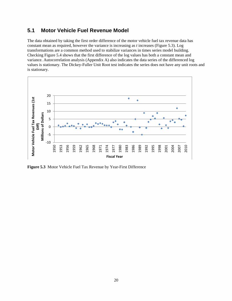
5.1 Motor Vehicle Fuel Revenue Model ......................................................................................... 20

5.2 Motor Vehicle License Fees ...................................................................................................... 23

5.3 Conclusion ................................................................................................................................. 26

6. SUMMARY ......................................................................................................................................... 27

REFERENCES .......................................................................................................................................... 29

APPENDIX A: RESULTS FROM WASHINGTON STATE DOT SURVEY .................................... 30

APPENDIX B. SURVEY FOR STATE DOT FINANCE MANAGERS ............................................. 32

APPENDIX C: THE ARIMA PROCEDURE AND SAS OUTPUT.................................................... 38

LIST OF TABLES Table 4.1 Type of Fuel Tax Revenue is Forecast (1 is yes, 0 is no) ...................................................... 9

Table 4.2 Model Technique Used by States for Forecasting Fuel Tax Revenue ................................. 10

Table 4.3 Fuel Revenue Tax Largest Forecast Error ........................................................................... 10

Table 4.4 Normal Forecasting Errors ................................................................................................... 11

Table 4.5 Variables Used in Motor Fuel Tax Revenue Forecasting Modeling .................................... 11

Table 4.6 Years with Highest Forecast Error for Motor Fuel Tax Revenue ........................................ 12

Table 4.7 Type of Model used to Forecast Motor Vehicle Licenses and Registration Fees ................ 13

Table 4.8 Frequency of Forecasting for Motor Vehicle Licenses and Registration Fees .................... 14

Table 4.9 Largest Forecast Error for Vehicle License and Registration Fees ...................................... 14

Table 4.10 Years with the Largest Forecast Errors for Vehicle Licenses and Registration Revenue .... 15

Table 4.11 Most Common Error Level in Forecasting Vehicle Licenses and Registration ................... 15

Table 4.12 Variables Used in Forecasting for Motor Vehicle License and Registration Fees .............. 16

Table 5.1 Fuel Tax Revenue Forecasting Results ................................................................................ 22

Table 5.2 Actual and Forecast Values with Confidence Interval ......................................................... 23

Table 5.3 Model Estimates for Vehicle Registration and License Fees ............................................... 24

Table 5.4 Actual Value and Forecasts for Vehicle License Revenues ................................................. 25

LIST OF FIGURES Figure 5.1 Motor Vehicle Fuel Tax Revenues by Year ......................................................................... 19

Figure 5.2 Motor Vehicle License Revenues by Year........................................................................... 19

Figure 5.3 Motor Vehicle Fuel Tax Revenue by Year-First Difference................................................ 20

Figure 5.4 Log of Motor Vehicle Fuel Tax Revenues by Year and First Difference ............................ 21

Figure 5.5 Motor Vehicle Fuel Tax Revenues by Year ......................................................................... 22

Figure 5.6 Motor Vehicle License Revenues by Year and Second Difference ..................................... 23

Figure 5.7 Log of Motor Vehicle License Revenues by Year and Second Difference ......................... 24

Figure 5.8 Motor Vehicle License Revenues by Year .......................................................................... 25

1

1. BACKGROUND For more than 30 years research efforts across the country have been searching for a model that would provide a reasonable estimate of fuel demand. Economic shocks of recession or spiking oil/fuel prices may render usually reliable forecast worthless. Finding a method to forecast through all economic conditions is difficult and no model can account for all variables. State departments of transportation (DOT) face the difficult task of predicting revenue and estimating cash flow. Without a reasonably accurate picture of revenue it is difficult to budget. Most states have models in place to estimate revenue based on statistical and/or econometric modeling. Econometric models consisting of historical data can be developed to estimate revenues on an annual or quarterly basis. Fuel tax revenues and vehicle registration fees represent a large portion of the state transportation revenue collected and provide matching funds for federal sources. Because of reliance on federal sources, uncertainty and complexity exist at state departments of transportation (DOTs) in determining and estimating revenue and cash flow. Federal funds require matching funds or “Obligation Authority” and it is imperative that the state maximize the use of federal funds, but this may be difficult in the face of uncertainty of revenue collections. States use different systems to determine revenue, cash flow and/or balances. For sound decision making it is imperative that methods be employed to provide an accurate picture of the current financial situation. Methods used by other state DOTs or other state agencies across the country may provide a clear picture of current and future revenue collections. Methods or models may exist at other state agencies that go beyond current methods being used in North Dakota. These methods may provide a more accurate and transparent measure of what these balances are now and in the future. In addition different methods to determine cash balances and needs may exist at DOTs or other state agencies. A survey of state DOTs to determine forecasting methods may provide information useful in development of a system for forecasting and managing cash flow. In this three section report, the first section is a literature review focusing on state methods of forecasting for revenues from fuel tax receipts and license and registration fees. The second part reports on a survey conducted by researchers to ascertain the different forecasting methods and problems other states face. The third sections reports on the models forecasting motor fuel tax revenue and license and registration fee revenue for North Dakota.

2

2. OBJECTIVE This project has two primary objectives. The first objective is to survey state DOTs to determine methods used by State DOTs in forecasting fuel tax revenues and license and registration fees collect and some information on other states management of cash flows and balances. The second objective is to develop models to forecast revenues from motor fuel taxes and registration fee revenues.

3

3. LITERATURE REVIEW This section looks at highway user revenue forecasting models. Examining the literature may identify some best practices used by state departments of transportation and federal agencies. These models may have been developed by DOTs, consultants and/or academia. States budgets are typically proposed by the governor’s office and then it is up to the legislature to go through the process of establishing the budget which may or may not reflect the wishes of the governor. 3.1 State Forecasting Models This section describes models developed by state DOTs to forecast highway user tax revenues in Virginia, Arizona, California, Indiana, and Wisconsin. Pressures for forecasting accuracy are never greater than during periods of economic recession. Inaccurate forecasts make it nearly impossible to project with any certainty what revenues will be. This results in fiscal shortfalls which may start at the federal level and end up at local levels. 3.1.1 California Department of Transportation: Motor Vehicle Stock, Travel

and Fuel Forecast The California Motor Vehicle Stock, Travel and Fuel Forecast (MVSTAFF) report is published annually by the California Department of Transportation (Caltrans) (California Department of Transportation, California Motor Vehicle Stock, Travel and Fuel Forecast, December 2006). This forecast and report has been published since 1984. The MVSTAFF procedure is repetitive estimating:

• motor vehicle stock • average number of currently registered vehicles by six body types • two fuel types • 25 model years • fuel economy of the total fleet • each model year fleet • vehicle travel (in miles) • fuel consumption for the total fleet

California was developing a new model in 2010 and the outcome is unknown at this time. 3.1.2 Arizona Department of Transportation Revenue Forecasting Process Arizona taxes motor fuels and collects a variety of fees relating to the registration and operation of motor vehicles. These revenues are deposited into the Arizona Highway User Revenue Fund (HURF) and distributed to cities, towns and counties in the State and the State Highway Fund. These funds represent the state’s share of revenue for highway construction, improvements and other related expenses (Arizona Department of Transportation, Update of the Highway User Revenue Fund and Maricopa Regional Area Road Fund Forecasting Models, prepared by HDR|HLB Decision Economics Inc., July 2005).

4

The Arizona Department of Transportation (ADOT) uses a regression model to forecast revenues. ADOT has been using a Risk Analysis Process (RAP) since 1992. The RAP is a probability analysis with independent evaluation of variables using experts. The result is forecasts associated with probabilities. Variables included in the model are fuel efficiency, real capita personal income, population growth, and wage and salary growth. The model does not include the price of fuel (Statewide Fuel Consumption Forecast Models, Arizona State DOT, 2010). 3.1.3 Wisconsin Department of Transportation The Wisconsin Department of Transportation (WisDOT) was one of the first to forecast revenue using an econometric model of gasoline demand. The model is a multiple-time-series resulting in a forecast of state tax revenues (HDR/HLB Decision Economics Inc., 2010). An econometric model using a single equation of quarterly gasoline demand was developed within a multiple-time-series framework. Gasoline demand is a function of real gasoline price, real disposable income, vehicle fleet, and fuel efficiency. Dummy variables account for times of shock in the economy or low supply or high prices. The model uses a seasonal autocorrelation term. The model uses a log-linear function allowing parameters to be interpreted as short-run elasticities. VMT was used to estimate gasoline consumption (HDR/HLB Decision Economics Inc., 2010). 3.1.4 Indiana Department of Transportation: INDOTREV The Indiana Department of Transportation (INDOT) has been using the INDOTREV software to generate long-term highway revenue forecasts since the1990s. The software was designed cooperatively by INDOT, Purdue University and the Federal Highway Administration. A key characteristic of INDOTREV is that it accounts for the vehicle mix. The software can also provide revenue projections under various tax policies (Varma, A., Sinha, K.C., and Spalding, J.L., The Development of A Highway Revenue Forecasting Model for Indiana, Joint Highway Research Project, Purdue University, 1992). Indiana highway revenues are separated into seven major categories: registration, driver license, international registration plan, gasoline tax, special fuel tax, motor carrier surtax, and motor carrier fuel use tax. Registration revenue is divided into seven motor vehicle categories: automobiles, motorcycles, light duty trucks, tractors, buses, trailers, and semitrailers. Light duty trucks, tractors, trailers, and semitrailers are further divided into farm and non-farm categories. Separate regression equations are used for each category of motor vehicle to estimate vehicle registration (number of vehicles registered) and vehicle use (number of vehicle miles traveled). The state socioeconomic environment (population, gross state product, and per capita personal income) with an emphasis on the per capita personal income, are key explanatory variables of personal vehicle travel (HDR/HLB Decision Economics Inc., 2010). The fleet fuel efficiency was determined by estimating the proportion of vehicles by age and the relative miles of travel for the various ages. Fuel consumption (in millions of gallons) is estimated by dividing VMT of each vehicle category by its respective fleet fuel efficiency. All fuel consumption by automobiles and motorcycles was considered to be gasoline, 96 percent of the light-duty truck fuel consumption is considered gasoline. Fuel consumed by tractors, buses and the remaining 4 percent of light-duty trucks is estimated to be special fuel.

5

3.1.5 Virginia Cash Forecasting Until 2002 the Virginia Department of Transportation had a forecasting model but chose not to make operating or financing decisions from the model estimates or use it in the development of its Six Year Program. The model was run only to determine cash flow status. Using this analysis in this way only provided analysis for individual projects. Using the model in this way was problematic. Cash shortages for projects became common, leading to borrowing between funds within the department. The author that critiqued the Virginia model stated that failure to use forecasting as an integral part of planning has contributed to VDOTs cash shortfalls. With the passing of the Virginia Transportation Act, VDOT attempted to use the old forecasting model without success. The model was not designed adequately, and financial planners had to adjust the information manually. The old model was eventually scrapped. VDOT used a consultant to design and implement a new cash forecasting tool. The cash forecasting database updates the project payouts, takes the balance of the contract, and shortens or lengthens the project schedule to match the award amount. In addition, the new database is able to handle the multiple funding sources created by the Virginia Transportation Act. According to the article, not all has been solved and some issues are under review. One of the biggest problems is lack of information-sharing among divisions. 3.1.6 Washington Fuel Consumption Forecast Methods The final statewide econometric gasoline and diesel consumption forecast models were determined after considering various forecast model specifications. Quarterly and annual fuel consumption models will be used in the new forecasting methodology. Both final quarterly and annual gas and diesel consumption models are of log-log functional form. O The gasoline consumption quarterly model includes the log of the following independent variables:

Washington non-agricultural employment Composite variable of Washington gas prices and fuel efficiency Dummy variable for periods of severe oil supply shortages

O Gasoline consumption annual model includes the log of the following independent variables: Washington non-agricultural employment (first difference) Washington population (first difference) Composite variable of Washington gas prices and fuel efficiency

O Diesel consumption quarterly model includes the log of the following independent variables: Washington employment – trade, transportation and utilities sectors Washington real personal income

O Diesel consumption annual model includes the log of the following independent variables: Washington employment – trade, transportation and utilities sectors Washington real personal income

Each independent variable has its own separate and distinct forecast which can be used to project fuel consumption. These regression models were selected because they had the best overall fit, significant t-statistics and other critical statistics. In addition, the economic variables in the models had a close nexus to fuel consumption. These new forecast models will assist us in separating the near-term and long-term impacts on fuel consumption (Statewide Fuel Consumption Forecast Models, Washington State DOT, 2010).

6

3.1.7 Other Forecasting Models This section reports on reviews of other forecasting models. A model developed by the Department of Energy is reviewed. Methods of modeling are also presented. 3.1.8 U.S. Department of Energy Short-Term Integrated Forecasting System This Short-Term Integrated Forecasting System (STIFS) model was originally developed in the early 1970s by the Bureau of Mines. The model has been modified from its original format to include price shocks and other factors that have come about since inception. The model is maintained by the Energy Information Administration (EIA), a unit of the U.S. Department of Energy (DOE). The model generates short-term and monthly forecasts of U.S. supplies, demands, imports, stocks, and prices of different energy products. The forecasts support many publications which include the monthly Short-Term Energy Outlook. The EIA also offers a spreadsheet model intended for sensitivity analysis (U.S. Energy Information Administration, 2010) The PC Short-Term Energy Model (PC-STEO) presents EIA’s latest monthly national energy forecast using an Excel-like presentation. The PC-STEO model provides a simulation engine that updates the forecast to reflect changes made to the data. The STIFS model consists of more than 300 equations where 100 are estimated and divided into seven sub-models: Petroleum Products Supply Model; Petroleum Products Demand Model; Other Petroleum Products Demand Model; Energy Prices Model; Electricity Model; Coal Model; and Natural Gas Model. The equations are estimated with the ordinary least squares method (U.S. Energy Information Administration, 2010). Within the Petroleum Products Demand Model the demand for motor gasoline is estimated by means of two equations: motor gasoline deliveries (barrels) and highway travel activity (miles traveled). The first equation requires projected highway travel data from the second one. The determinants of motor gasoline deliveries are highway travel, inflation-adjusted average retail motor gasoline prices, and several dummy variables to account for seasonality in gasoline deliveries, modifications to the Reid Vapor Pressure1

(RVP) standards previously implemented, and the implementation of reformulated gasoline regulations since 1995. Highway travel is explained by real disposable income, inflation-adjusted cost per mile (i.e., retail gasoline price) with a lag of 12 months and a polynomial degree of two2 ,

and several dummy

variables pertaining to weather-related disruptions in travel and changes in reporting methodology for vehicle miles traveled (U.S. Energy Information Administration, 2010). A criticism of the model is that it does not account for average fuel mileage in the fleet. Its motor gasoline deliveries equation does include real gasoline price through which it indirectly accounts for consumer selection in reacting to fuel pricing.

1 RVP is a method of determining vapor pressure of gasoline and other petroleum products. It is widely used in the petroleum industry as an indicator of the volatility (vaporization characteristics) of gasoline. 2 Polynomial distributed lags (PDL) are used to reduce the effects of collinearity in distributed lag settings by imposing a particular shape on the lag coefficients. The specification of a polynomial distributed lag has three elements: the length of the lag (the number of time periods it covers), the degree of the polynomial (the highest power in the polynomial), and the constraints on the lag coefficients. A near end constraint says that the immediate effect of x on y is zero, whereas a far end constraint says that the effect of x on y dies off at the end. It is also possible to impose both constraints or no constraint at all.

7

3.1.9 Kouris (1982) A study by George Kouris of the Organization for Economic Cooperation and Development (OECD), International Energy Agency (IEA) in 1982 provides an overview of the issues involved in estimating fuel demand for road transport in the United States (Kouris, G., “Fuel Consumption for Road Transport in the U.S.A.,” Energy Economics, Volume 5, Issue 2, April 1983). Kouris reviewed previous approaches which he classifies into reduced form and structural form approaches. The reduced form determines that fuel demand is mostly a function of income and price but is also sensitive to other variables such as temperature, consumer preferences, and social emulation, along with other less important variables. The structural form focuses on the economy of the vehicle fleet and the rate of use. The two approaches are interrelated. Kouris also provided elasticities from previous studies for both the short-and long-run periods. Of particular interest is the analysis of the causal factors of fuel economy trends and the ability to forecast them. Existing regression-based models used to predict fleet fuel economy were described and a comparison of resulting elasticity coefficients was presented. References cited by the author represent a good cross section of research up to the early 1980s. 3.1.9 Gillen (1999) Gillen assessed performance of states forecast revenues from taxes and fees levied on highway users and whether the models they employ in forecasting revenues are adequate. Gillen distinguishes three broad forecasting approaches. A simple approach would be to develop a model that uses previous values of revenues in each category perhaps with a weighting structure on more recent values. This approach simply matches a function to the data and extrapolates the values to create a forecast (Gillen, David, “Estimating Revenues from User Charges, Taxes and Fees: Identifying Information Requirements,” August 1999). A second approach would utilize some econometric time series techniques, such as the Box-Jenkins or ARIMA. Univariate Box-Jenkins models are sophisticated extrapolation methods using past values to generate forecasts. When there is a lack of information or specification errors make econometric models impractical, the Box-Jenkins model is considered a superior form of time-series forecasting. The third approach, causal forecasting, develops an econometric model that explains the underlying causes or sources of variation in the factors that affect revenues from fuel taxes and registration fees. These would utilize relevant demographic and economic variables in a set of behavioral equations to produce the forecast. It is the richest approach because once the model parameters are estimated they can be used to develop forecasts of the dependent variables. The models used by most states to forecast travel and other variables affecting fuel tax revenues are accounting identities or other simple statistical relationships which forecasts components of revenues. They are simplistic and non-behavioral. One common but disturbing feature of such models is their assumption that the demands for travel, vehicles, and fuel are non-responsive to changes in the social, demographic and economic variables. This leads to the implication that there is no response of fuel use to changes in fuel price, either through the number and type of vehicles owned or the amount each one is driven; in economic terms, the demand for fuel is assumed to be perfectly inelastic. Gillen proposed a modeling approach that could serve as the basis for all states to develop forecasts. His approach consists of a system of three equations: two relationships (VMT and fleet fuel efficiency) and one accounting identity (total fuel consumption). This would provide the requisite information to forecast fuel tax and registration fee and other fee revenues. The first two equations are estimated via regression analysis, while the third equation combines the results of the first two.

8

The main determinants of VMT are assumed to be household income, vehicle price, fuel price, average fleet fuel efficiency, and average household size. Fleet fuel efficiency could be explained by personal income, fuel price and some vehicle technological factor to account for the continuing progress in engine design. Fuel consumption would then be obtained by dividing VMT by fleet fuel efficiency. The level of disaggregation of highway user revenues varies from state to state. Most forecasting models rely on a regression analysis of vehicle ownership and vehicle use; The level of modeling sophistication varies from state to state, from the simplistic (e.g., trend model) to the relatively sophisticated (e.g., multiple-time-series framework). 3.1.10 Conclusion The literature reveals that most states are forecasting revenues using either statistical or econometric models. These models provide states with valuable information for budgeting and meeting or setting their obligation authority. States use different approaches. In forecasting for fuel revenue, some states estimate VMT and fuel efficiency of the fleet and the fleet disposition. Other states use historical and other variables such as GSP, income, employment etc. as variables for the forecasting models. Most models have evolved over time and states are focusing on continuous improvement in their forecasting models to provide them with the best results during economic growth or recession. Gillen provided insight in the 1990s with regard to the problems with states’ forecasts of fuel revenue. Some states have employed his approach. One approach is using experts or consensus forecasts to at least set the parameters of the forecast in the face of economic or political or social changes. Others states are using some more complex modeling and are forecasting more frequently in an attempt to increase accuracy. The next section provides responses from states surveyed about their forecasting methodology, results, problems and errors. This survey was sent to all 50 states with 10 states responding.

9

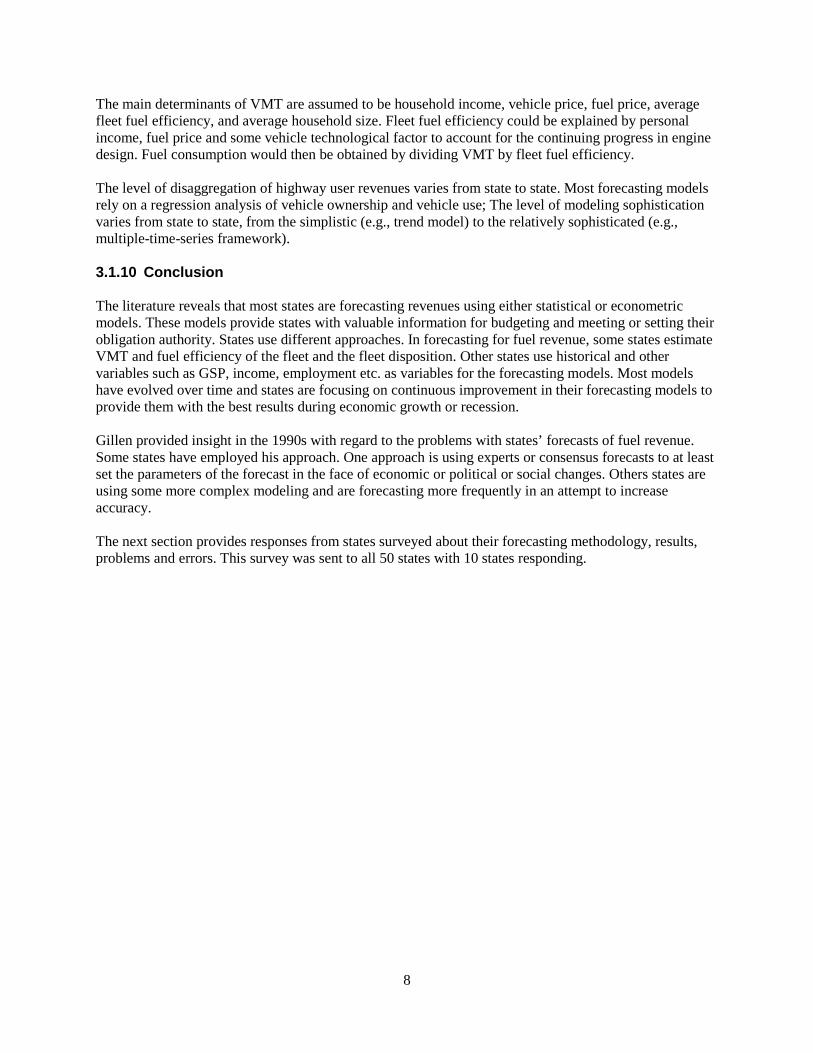
4. SURVEY Forecasting revenue and matching revenue to expenditures is a balancing act. A survey of state DOTs to determine forecasting methods may provide insight into a process that will work in North Dakota. A survey was sent to all 50 state departments of transportations’ finance divisions to gauge their use of forecasting for revenues from fuel tax collections and vehicle registration and licensing fees (Appendix I). Ten states responded to the survey: Nebraska, Missouri, Washington, South Dakota, Arizona, Nevada, South Carolina, Mississippi, Kansas, and North Carolina. Contact information was asked for and received from the 10 respondents. 4.1 Motor Fuel Revenue Forecasting The first question simply asked whether the DOT developed a forecast for motor fuel revenue and all responded that they did. The second question asked if they separated the forecast for different types of fuel. Eight states do separate forecasts for different fuel types and two do not. The third question asked what types of fuel revenues are forecast. Eighty percent reported forecasting for diesel and gasoline while one state forecast for airplane fuel and two for jet fuel. South Dakota and South Carolina left the question blank. Table 4.1 Type of Fuel Tax Revenue is Forecast (1 is yes, 0 is no).

State Diesel Gasoline Nat Gas Electricity Ethanol

Airplane Fuel

Jet Fuel Coal Other

Nebraska 1 1 0 0 0 0 0 0 0 Missouri 1 1 0 0 0 0 1 0 0 Washington 1 1 0 0 0 0 0 0 0 South

Dakota 0 0 0 0 0 0 0 0 0

Arizona 1 1 0 0 0 0 0 0 0 Nevada 1 1 0 0 0 0 0 0 0 South

Carolina 0 0 0 0 0 0 0 0 0

Michigan 1 1 0 0 0 1 1 0 0 Kansas 1 1 0 0 0 0 0 0 0 North

Carolina 1 1 0 0 0 0 0 0 0

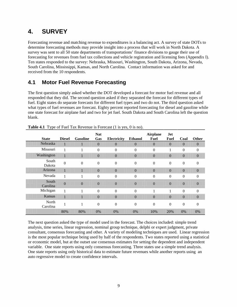
80% 80% 0% 0% 0% 10% 20% 0% 0% The next question asked the type of model used in the forecast. The choices included: simple trend analysis, time series, linear regression, nominal group technique, delphi or expert judgment, private consultant, consensus forecasting and other. A variety of modeling techniques are used. Linear regression is the most popular technique being used by half of the respondents. Two states reported using a statistical or economic model, but at the outset use consensus estimates for setting the dependent and independent variable. One state reports using only consensus forecasting. Three states use a simple trend analysis. One state reports using only historical data to estimate future revenues while another reports using an auto regressive model to create confidence intervals.

10

Table 4.2 Model Technique Used by States for Forecasting Fuel Tax Revenue (1 indicates use, 0 not used)

Simple Trend

Time Series

Linear Regression Simulation

Nominal Group Delphi

Private Consult Consensus Other

Nebraska 1 0 0 0 0 0 0 0 0 Missouri 0 0 1 0 0 0 0 0 0

Washington 0 1 0 0 0 0 0 0 0 South

Dakota 0 0 1 0 0 0 0 0 0

Arizona 0 0 1 0 0 0 0 1 0 Nevada 1 1 1 0 0 0 0 0 0

South Carolina 1 0 0 0 0 0 0 0 0

Michigan 0 0 0 0 0 0 0 0 1 Kansas 0 0 0 0 0 0 0 1 0

North Carolina 0 0 1 0 0 0 0 1 0

30% 20% 50% 0% 0% 0% 0% 30% 10% The next question asked the frequency of their forecast. These responses covered all the options with 4 of the 10 reporting annual, 3 reporting semi-annual, 2 reporting quarterly and 1 reporting forecasting monthly. The next question asked about states’ largest forecast error. The options ranged from less than 1% to greater than 7%. Two states or 20% reported no more than 2% forecast error as the high while Arizona reported an 8.9% error over the forecast for 2009. Two states reported errors of between 3% and 4%. The weighted average of forecast error was 3.5% with a range of greater than 1% to greater than 7%. The state that reported the error greater than 7% commented that the error was 8.9% in 2009. Half of the states reported their largest forecast error was less than 4%. Table 4.3 Fuel Revenue Tax Largest Forecast Error

< 1%

1% < > 2%

2% < > 3%

3% < > 4%

4% < > 5%

5% < > 6%

6% < > 7%

> 7% Other

Nebraska 0 0 1 0 0 0 0 0 0 Missouri 0 1 0 0 0 0 0 0 0

Washington 0 0 0 0 0 0 0 0 0 South

Dakota 0 0 0 1 0 0 0 0 0

Arizona 0 0 0 0 0 0 0 1 0 Nevada 0 0 0 0 0 0 0 0 1

South Carolina 0 0 0 1 0 0 0 0 0

Michigan 0 0 0 0 0 0 0 1 0 Kansas 0 0 0 0 1 0 0 0

North Carolina 0 1 0 0 0 0 0 0 0

0% 20% 10% 20% 0% 10% 0% 20% 10%

11

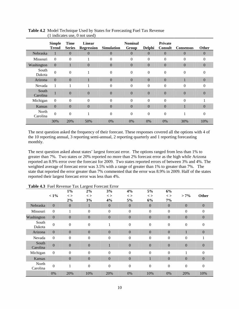
Next respondents were asked about their most frequent forecast error. Half of the respondents reported errors of between 2% and 3% are common. All respondents reported common errors at less than 4%. Table 4.4 Normal Forecasting Errors

State < 1% 1% < > 2%

2% < > 3%

3% < > 4%

4% < > 5%

5% < > 6%

6% < > 7%

>7%

Nebraska 0 0 1 0 0 0 0 0 Missouri 1 1 0 0 0 0 0 0

Washington 0 0 0 0 0 0 0 0 South

Dakota 0 0 1 0 0 0 0 0

Arizona 1 0 0 0 0 0 0 0 Nevada 0 0 0 1 0 0 0 0

South Carolina 0 0 1 0 0 0 0 0

Michigan 0 0 0 0 0 0 0 0 Kansas 0 0 1 0 0 0 0 0

North Carolina 0 1 1 0 0 0 0 0

20% 20% 50% 10% 0% 0% 0% 0% Question 8 asked respondents if they used external variables in their modeling of Motor Fuels Tax Revenue. All respondents answered the question and 60% replied that they used external variable while 40% responded that they do not. The next question asked respondents about those variables and the table below shows that only 40% use fuel price as a predictor of motor fuels tax revenue collections and only one uses gross state product (GSP). Table 4.5 Variables Used in Motor Fuel Tax Revenue Forecasting Modeling

State

Fuel Price GDP GSP

Consumer Confidence Unemployment

Disposable Income Other

Nebraska 1 0 0 0 0 0 1 Missouri 0 0 1 0 0 1 1

Washington 1 0 0 0 1 0 0 South

Dakota 0 0 0 0 0 0 1

Arizona 1 0 0 0 0 0 1 Nevada 0 0 0 0 0 0 1

South Carolina 0 0 0 0 0 0 1

Michigan 0 0 0 0 0 0 1 Kansas 0 0 0 0 0 0 0

North Carolina 1 0 0 0 0 0 0

40% 0% 10% 0% 10% 10% 70%

12

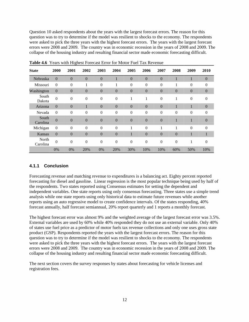
Question 10 asked respondents about the years with the largest forecast errors. The reason for this question was to try to determine if the model was resilient to shocks to the economy. The respondents were asked to pick the three years with the highest forecast errors. The years with the largest forecast errors were 2008 and 2009. The country was in economic recession in the years of 2008 and 2009. The collapse of the housing industry and resulting financial sector made economic forecasting difficult. Table 4.6 Years with Highest Forecast Error for Motor Fuel Tax Revenue

State 2000 2001 2002 2003 2004 2005 2006 2007 2008 2009 2010

Nebraska 0 0 0 0 1 0 0 0 1 1 0 Missouri 0 0 1 0 1 0 0 0 1 0 0

Washington 0 0 0 0 0 0 0 0 0 0 0 South

Dakota 0 0 0 0 0 1 1 0 1 0 0

Arizona 0 0 1 0 0 0 0 0 1 1 0 Nevada 0 0 0 0 0 0 0 0 0 0 0

South Carolina 0 0 0 0 0 0 0 0 1 1 0

Michigan 0 0 0 0 0 1 0 1 1 0 0 Kansas 0 0 0 0 0 1 0 0 0 1 1

North Carolina 0 0 0 0 0 0 0 0 0 1 0

0% 0% 20% 0% 20% 30% 10% 10% 60% 50% 10% 4.1.1 Conclusion Forecasting revenue and matching revenue to expenditures is a balancing act. Eighty percent reported forecasting for diesel and gasoline. Linear regression is the most popular technique being used by half of the respondents. Two states reported using Consensus estimates for setting the dependent and independent variables. One state reports using only consensus forecasting. Three states use a simple trend analysis while one state reports using only historical data to estimate future revenues while another reports using an auto regressive model to create confidence intervals. Of the states responding, 40% forecast annually, half forecast semiannual, 20% report quarterly and 1 reports a monthly forecast. The highest forecast error was almost 9% and the weighted average of the largest forecast error was 3.5%. External variables are used by 60% while 40% responded they do not use an external variable. Only 40% of states use fuel price as a predictor of motor fuels tax revenue collections and only one uses gross state product (GSP). Respondents reported the years with the largest forecast errors. The reason for this question was to try to determine if the model was resilient to shocks to the economy. The respondents were asked to pick the three years with the highest forecast errors. The years with the largest forecast errors were 2008 and 2009. The country was in economic recession in the years of 2008 and 2009. The collapse of the housing industry and resulting financial sector made economic forecasting difficult. The next section covers the survey responses by states about forecasting for vehicle licenses and registration fees.

13

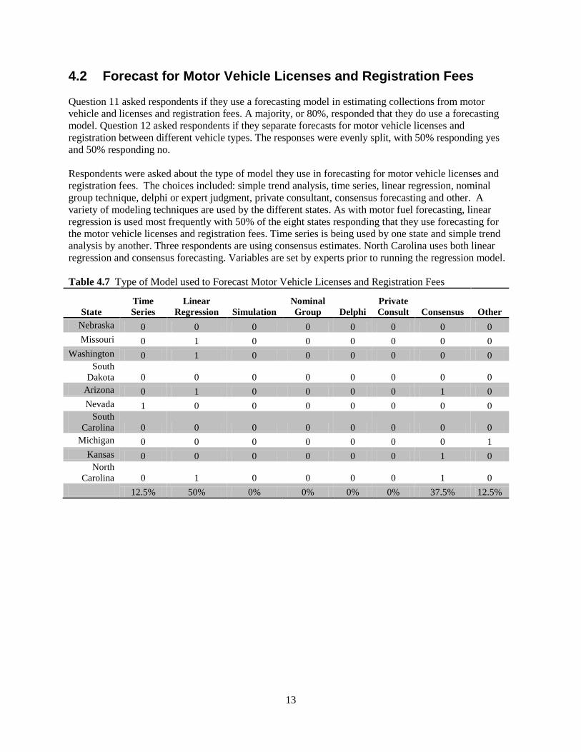
4.2 Forecast for Motor Vehicle Licenses and Registration Fees Question 11 asked respondents if they use a forecasting model in estimating collections from motor vehicle and licenses and registration fees. A majority, or 80%, responded that they do use a forecasting model. Question 12 asked respondents if they separate forecasts for motor vehicle licenses and registration between different vehicle types. The responses were evenly split, with 50% responding yes and 50% responding no. Respondents were asked about the type of model they use in forecasting for motor vehicle licenses and registration fees. The choices included: simple trend analysis, time series, linear regression, nominal group technique, delphi or expert judgment, private consultant, consensus forecasting and other. A variety of modeling techniques are used by the different states. As with motor fuel forecasting, linear regression is used most frequently with 50% of the eight states responding that they use forecasting for the motor vehicle licenses and registration fees. Time series is being used by one state and simple trend analysis by another. Three respondents are using consensus estimates. North Carolina uses both linear regression and consensus forecasting. Variables are set by experts prior to running the regression model. Table 4.7 Type of Model used to Forecast Motor Vehicle Licenses and Registration Fees

State

Time Series

Linear Regression Simulation

Nominal Group Delphi

Private Consult Consensus Other

Nebraska 0 0 0 0 0 0 0 0 Missouri 0 1 0 0 0 0 0 0

Washington 0 1 0 0 0 0 0 0 South

Dakota 0 0 0 0 0 0 0 0 Arizona 0 1 0 0 0 0 1 0 Nevada 1 0 0 0 0 0 0 0

South Carolina 0 0 0 0 0 0 0 0

Michigan 0 0 0 0 0 0 0 1 Kansas 0 0 0 0 0 0 1 0

North Carolina 0 1 0 0 0 0 1 0

12.5% 50% 0% 0% 0% 0% 37.5% 12.5%

14

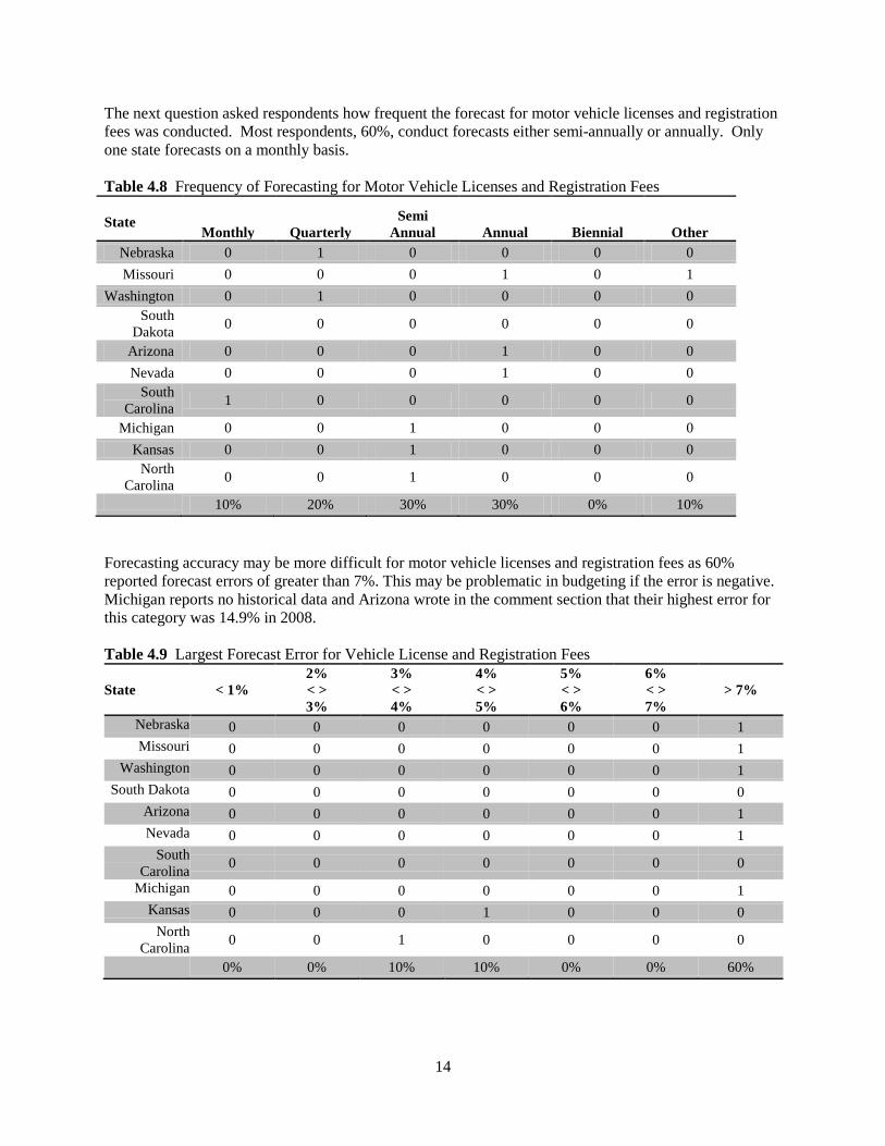
The next question asked respondents how frequent the forecast for motor vehicle licenses and registration fees was conducted. Most respondents, 60%, conduct forecasts either semi-annually or annually. Only one state forecasts on a monthly basis. Table 4.8 Frequency of Forecasting for Motor Vehicle Licenses and Registration Fees

State

Monthly Quarterly Semi

Annual Annual Biennial Other Nebraska 0 1 0 0 0 0 Missouri 0 0 0 1 0 1

Washington 0 1 0 0 0 0 South

Dakota 0 0 0 0 0 0

Arizona 0 0 0 1 0 0 Nevada 0 0 0 1 0 0

South Carolina 1 0 0 0 0 0

Michigan 0 0 1 0 0 0 Kansas 0 0 1 0 0 0

North Carolina 0 0 1 0 0 0

10% 20% 30% 30% 0% 10% Forecasting accuracy may be more difficult for motor vehicle licenses and registration fees as 60% reported forecast errors of greater than 7%. This may be problematic in budgeting if the error is negative. Michigan reports no historical data and Arizona wrote in the comment section that their highest error for this category was 14.9% in 2008. Table 4.9 Largest Forecast Error for Vehicle License and Registration Fees

State < 1%

2% < > 3%

3% < > 4%

4% < > 5%

5% < > 6%

6% < > 7%

> 7%

Nebraska 0 0 0 0 0 0 1 Missouri 0 0 0 0 0 0 1

Washington 0 0 0 0 0 0 1 South Dakota 0 0 0 0 0 0 0

Arizona 0 0 0 0 0 0 1 Nevada 0 0 0 0 0 0 1

South Carolina 0 0 0 0 0 0 0

Michigan 0 0 0 0 0 0 1 Kansas 0 0 0 1 0 0 0

North Carolina 0 0 1 0 0 0 0

0% 0% 10% 10% 0% 0% 60%

15

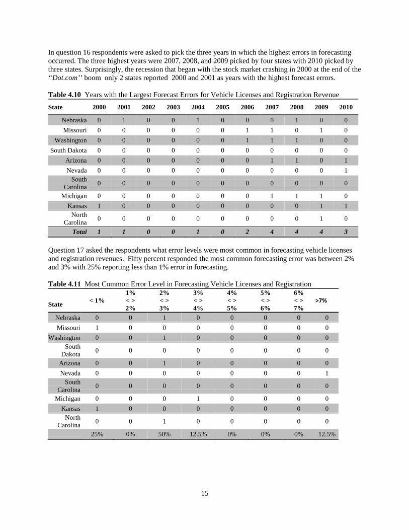
In question 16 respondents were asked to pick the three years in which the highest errors in forecasting occurred. The three highest years were 2007, 2008, and 2009 picked by four states with 2010 picked by three states. Surprisingly, the recession that began with the stock market crashing in 2000 at the end of the “Dot.com’’ boom only 2 states reported 2000 and 2001 as years with the highest forecast errors. Table 4.10 Years with the Largest Forecast Errors for Vehicle Licenses and Registration Revenue

State 2000 2001 2002 2003 2004 2005 2006 2007 2008 2009 2010

Nebraska 0 1 0 0 1 0 0 0 1 0 0 Missouri 0 0 0 0 0 0 1 1 0 1 0

Washington 0 0 0 0 0 0 1 1 1 0 0 South Dakota 0 0 0 0 0 0 0 0 0 0 0

Arizona 0 0 0 0 0 0 0 1 1 0 1 Nevada 0 0 0 0 0 0 0 0 0 0 1

South Carolina 0 0 0 0 0 0 0 0 0 0 0

Michigan 0 0 0 0 0 0 0 1 1 1 0 Kansas 1 0 0 0 0 0 0 0 0 1 1

North Carolina 0 0 0 0 0 0 0 0 0 1 0

Total 1 1 0 0 1 0 2 4 4 4 3 Question 17 asked the respondents what error levels were most common in forecasting vehicle licenses and registration revenues. Fifty percent responded the most common forecasting error was between 2% and 3% with 25% reporting less than 1% error in forecasting. Table 4.11 Most Common Error Level in Forecasting Vehicle Licenses and Registration

State < 1%

1% < > 2%

2% < > 3%

3% < > 4%

4% < > 5%

5% < > 6%

6% < > 7%

>7%

Nebraska 0 0 1 0 0 0 0 0 Missouri 1 0 0 0 0 0 0 0

Washington 0 0 1 0 0 0 0 0 South

Dakota 0 0 0 0 0 0 0 0

Arizona 0 0 1 0 0 0 0 0 Nevada 0 0 0 0 0 0 0 1

South Carolina 0 0 0 0 0 0 0 0

Michigan 0 0 0 1 0 0 0 0 Kansas 1 0 0 0 0 0 0 0

North Carolina 0 0 1 0 0 0 0 0

25% 0% 50% 12.5% 0% 0% 0% 12.5%

16

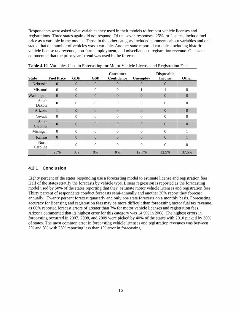
Respondents were asked what variables they used in their models to forecast vehicle licenses and registrations. Three states again did not respond. Of the seven responses, 25%, or 2 states, include fuel price as a variable in the model. Those in the other category included comments about variables and one stated that the number of vehicles was a variable. Another state reported variables including historic vehicle license tax revenue, non-farm employment, and miscellaneous registration revenue. One state commented that the prior years' trend was used in the forecast. Table 4.12 Variables Used in Forecasting for Motor Vehicle License and Registration Fees

State Fuel Price GDP GSP

Consumer Confidence Unemploy

Disposable Income Other

Nebraska 0 0 0 0 0 0 1 Missouri 0 0 0 0 1 1 0

Washington 0 0 0 0 0 0 0 South

Dakota 0 0 0 0 0 0 0

Arizona 1 0 0 0 0 0 0 Nevada 0 0 0 0 0 0 0

South Carolina 0 0 0 0 0 0 0

Michigan 0 0 0 0 0 0 1 Kansas 0 0 0 0 0 0 1

North Carolina 1 0 0 0 0 0 0

25% 0% 0% 0% 12.5% 12.5% 37.5% 4.2.1 Conclusion Eighty percent of the states responding use a forecasting model to estimate license and registration fees. Half of the states stratify the forecasts by vehicle type. Linear regression is reported as the forecasting model used by 50% of the states reporting that they estimate motor vehicle licenses and registration fees. Thirty percent of respondents conduct forecasts semi-annually and another 30% report they forecast annually. Twenty percent forecast quarterly and only one state forecasts on a monthly basis. Forecasting accuracy for licensing and registration fees may be more difficult than forecasting motor fuel tax revenue, as 60% reported forecast errors of greater than 7% for motor vehicle licenses and registration fees. Arizona commented that its highest error for this category was 14.9% in 2008. The highest errors in forecasting occurred in 2007, 2008, and 2009 were picked by 40% of the states with 2010 picked by 30% of states. The most common error in forecasting vehicle licenses and registration revenues was between 2% and 3% with 25% reporting less than 1% error in forecasting.

17

4.3 Cash Flow Question 19 asked respondents about problems in managing cash flow accounts. Forty percent of respondents claimed that they have problems with managing cash flow. Question 20 asked respondents if they use a model to forecast cash flow balances and 50% responded that they use a model while 40% responded that they did not use a model. One abstained from the yes or no answer and provided no explanation. Question 22 asked the respondents to explain the model used in their cash flow analysis. Models reported by respondents include: Time series as reported by one state, while another reported “Historical data combined with detailed statistical models to forecast future revenues. This data is then input into an Excel model to “cash out” all revenue and expenditures to ensure positive cash flow are maintained over a future 5-year period.” Simple trend analysis is used by two states and NCDOT uses an interactive cash model which incorporates data from a variety of revenue and expenditure models to produce a 10 year forecast of the departments’ financial position. While Kansas stated that it is “implementing a new Cash Forecasting Environment which is in process.”

18

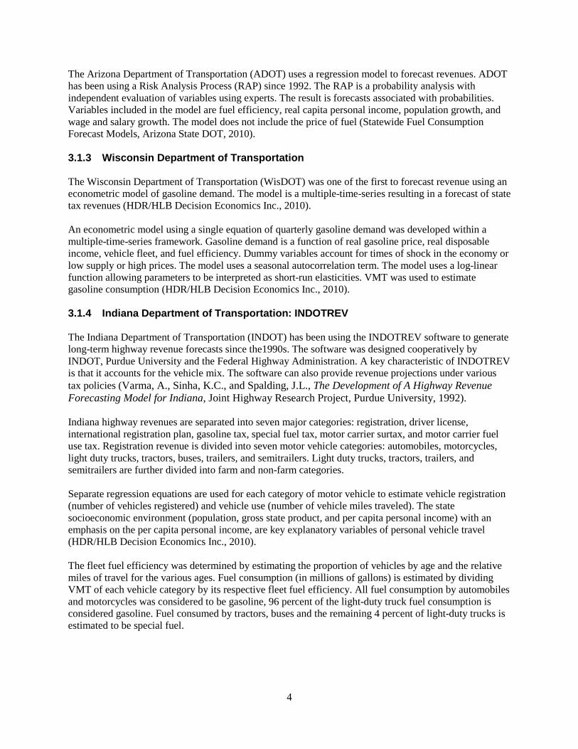
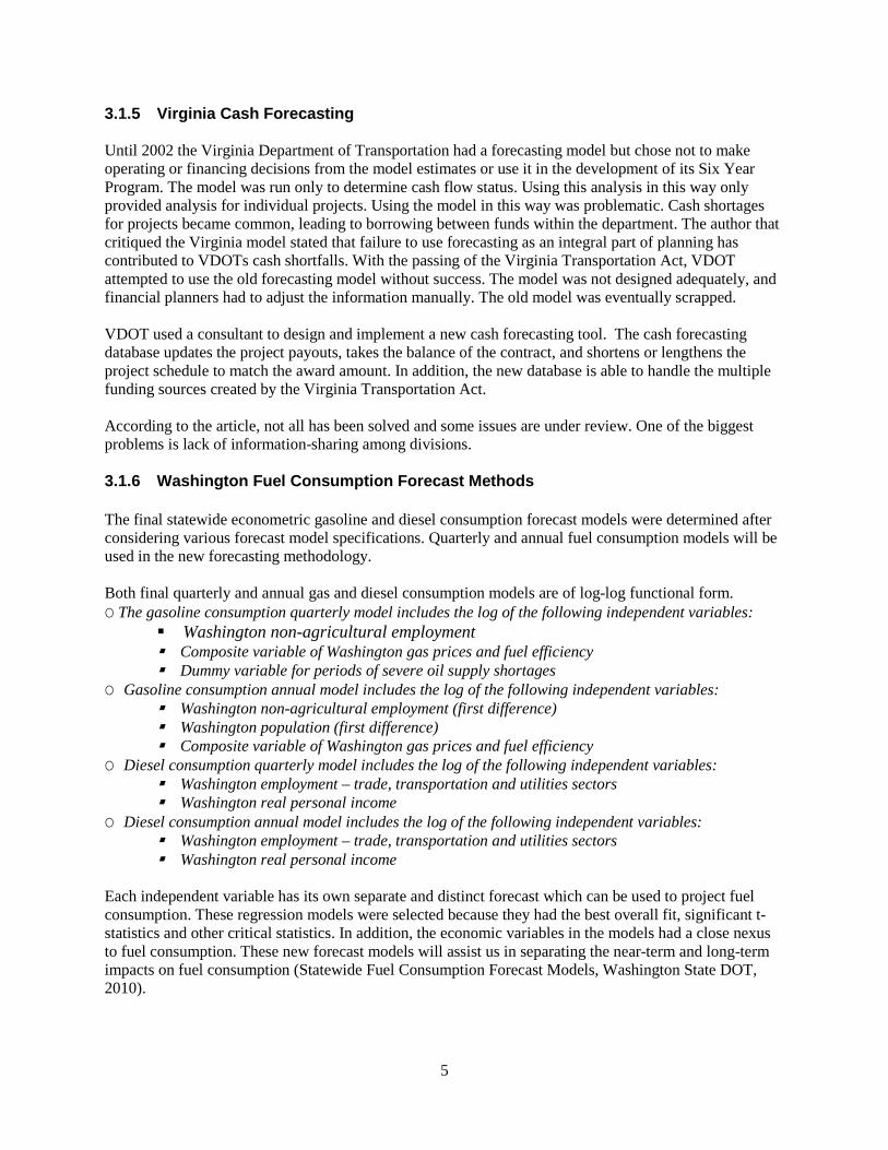
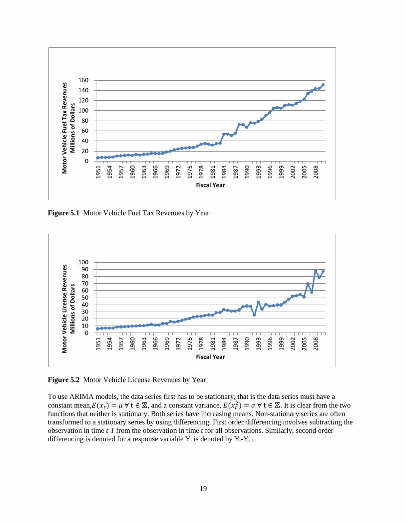
5. MODEL DEVELOPMENT Predicting revenues is important for any company or government agency. The North Dakota Department of Transportation receives a large part of it revenues from motor vehicle fuel taxes and motor vehicle license fees. The motor vehicle fuel revenue comes from taxes placed on each gallon of gasoline and diesel fuel sold in North Dakota. Vehicle license fees are fees associated with the sale and registrations of motor vehicles and off-road vehicles like ATVs, boats, snowmobiles, etc. The ability to accurately forecast the revenue from these sources aids the planning and budgeting process. States produce a variety of economic forecasts which directly and indirectly aid in estimating future revenues. Some states predict gasoline and diesel consumption, while others predict motor vehicle fuel revenue. Some produce motor vehicle license fee estimates which include vehicle licensing fees as well as driver’s license fees. The methods used by each state vary as greatly as the variables they are trying to estimate, ranging from expert opinion to time series models to extremely complex regressions models (HDR|HLB Decision Economics 2007, Shinn 2010, and Washington State DoT 2010). Each method has its strengths and weaknesses. Expert opinion is easiest to apply as it requires little data collection, is less costly, but is also less scientifically sound. Both times series and regression models are widely accepted for temporal forecasting. Time series models offer a more straightforward approach than regression models, but are often viewed as more trend-type models and not cause-and-effect-type models, since they only use combinations of previous results to produce future estimates. Time series models also offer an advantage when future forecasts are required such as in the case of predicting future revenues. The advantage is in the amount of data collection that needs to happen. Time series models can often be built with only the variable of interest. In our case, the variable is motor vehicle fuel taxes and motor vehicle license fees. To predict future values from regression models, the future values of each independent variable must be known or estimated. In a pure time series model, forecasting can be done with only prior knowledge of the stochastic variable. Data for these two revenue sources were obtained from the United State Census Bureau (US Census Bureau 2011). The data is collected as part of the Annual Survey of State Government Tax Collection and provides historical data back to 1951. The data includes categories of taxes and fees collected by state governments. Analysis included only information from the two variables mentioned above. Looking at the plotted values of motor vehicle fuel revenues in Figure 5.1 and vehicle license fees in Figure 5.2, reveals that both variables exhibit an increasing exponential function. Since both functions have very little fluctuations, they can most likely be easily modeled with an auto-regressive integrated moving average (ARIMA) model. This class model represents the most widely used and applicable class of time series modeling. Regression variables can also be added to the ARIMA model parameters and assessed for additional explanatory information.

19

Figure 5.1 Motor Vehicle Fuel Tax Revenues by Year

Figure 5.2 Motor Vehicle License Revenues by Year To use ARIMA models, the data series first has to be stationary, that is the data series must have a constant mean,𝐸(𝑥𝑡 ) = 𝜇 ∀ t ∈ 𝕫, and a constant variance, 𝐸(𝑥𝑡2) = 𝜎 ∀ t ∈ 𝕫. It is clear from the two functions that neither is stationary. Both series have increasing means. Non-stationary series are often transformed to a stationary series by using differencing. First order differencing involves subtracting the observation in time t-1 from the observation in time t for all observations. Similarly, second order differencing is denoted for a response variable Yt is denoted by Yt-Yt-2.

020406080

100120140160

1951

1954

1957

1960

1963

1966

1969

1972

1975

1978

1981

1984

1987

1990

1993

1996

1999

2002

2005

2008M

otor

Veh

icle

Fue

l Tax

Rev

enue

s M

illio

ns o

f Dol

lars

Fiscal Year

0102030405060708090

100

1951

1954

1957

1960

1963

1966

1969

1972

1975

1978

1981

1984

1987

1990

1993

1996

1999

2002

2005

2008

Mot

or V

ehic

le L

icen

se R

even

ues

Mill

ions

of D

olla

rs

Fiscal Year

20

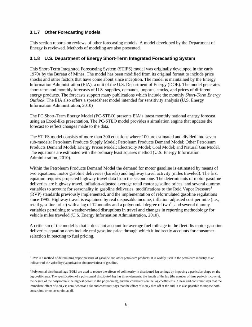
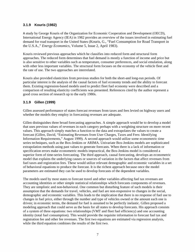
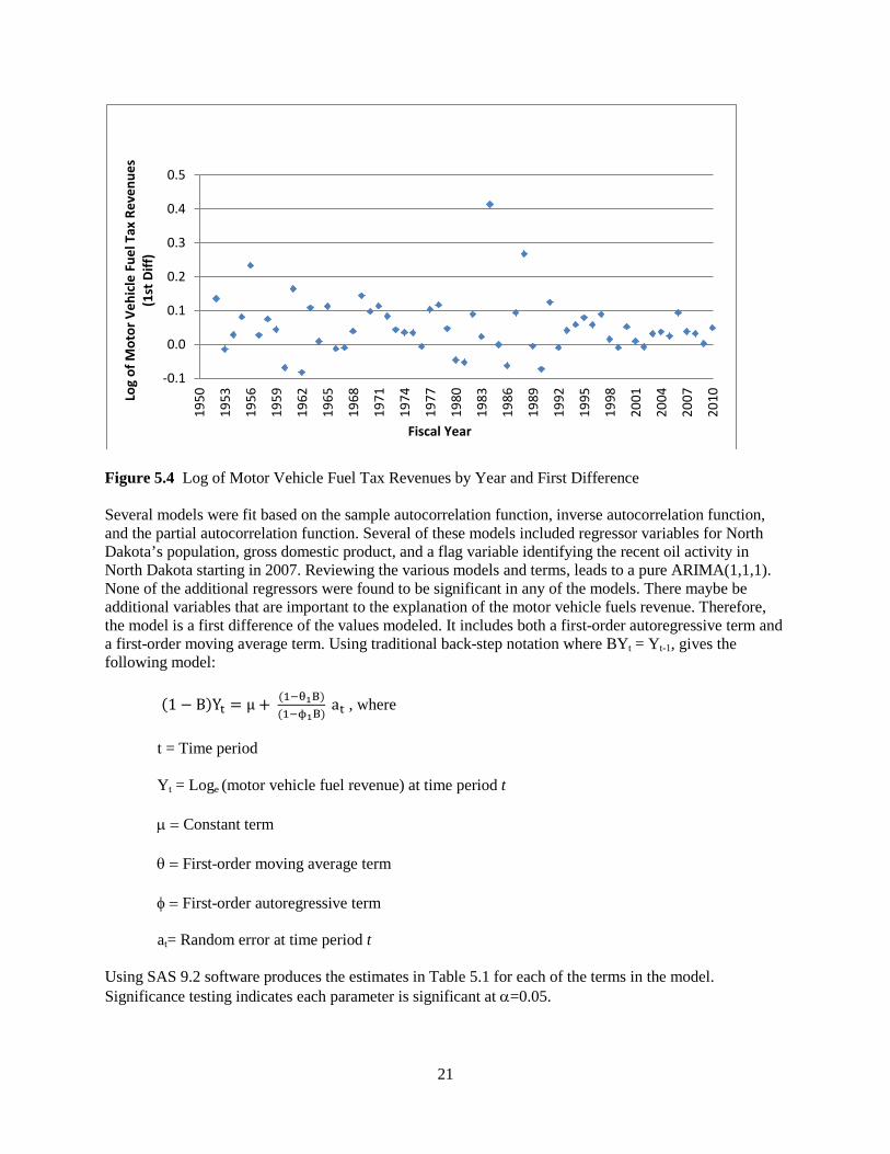
5.1 Motor Vehicle Fuel Revenue Model The data obtained by taking the first order difference of the motor vehicle fuel tax revenue data has constant mean as required, however the variance is increasing as t increases (Figure 5.3). Log transformations are a common method used to stabilize variances in times series model building. Checking Figure 5.4 shows that the first difference of the log values has both a constant mean and variance. Autocorrelation analysis (Appendix A) also indicates the data series of the differenced log values is stationary. The Dickey-Fuller Unit Root test indicates the series does not have any unit roots and is stationary.

Figure 5.3 Motor Vehicle Fuel Tax Revenue by Year-First Difference

-10

-5

0

5

10

15

20

1950

1953

1956

1959

1962

1965

1968

1971

1974

1977

1980

1983

1986

1989

1992

1995

1998

2001

2004

2007

2010

Mot

or V

ehic

le F

uel T

ax R

even

ues (

1st

Diff)

M

illio

ns o

f Dol

lars

Fiscal Year

21

Figure 5.4 Log of Motor Vehicle Fuel Tax Revenues by Year and First Difference Several models were fit based on the sample autocorrelation function, inverse autocorrelation function, and the partial autocorrelation function. Several of these models included regressor variables for North Dakota’s population, gross domestic product, and a flag variable identifying the recent oil activity in North Dakota starting in 2007. Reviewing the various models and terms, leads to a pure ARIMA(1,1,1). None of the additional regressors were found to be significant in any of the models. There maybe be additional variables that are important to the explanation of the motor vehicle fuels revenue. Therefore, the model is a first difference of the values modeled. It includes both a first-order autoregressive term and a first-order moving average term. Using traditional back-step notation where BYt = Yt-1, gives the following model:

(1 − B)Yt = µ + (1−θ1B)(1−ϕ1B)

at , where t = Time period

Yt = Loge (motor vehicle fuel revenue) at time period t

µ = Constant term θ = First-order moving average term φ = First-order autoregressive term at= Random error at time period t

Using SAS 9.2 software produces the estimates in Table 5.1 for each of the terms in the model. Significance testing indicates each parameter is significant at α=0.05.

-0.1

0.0

0.1

0.2

0.3

0.4

0.5

1950

1953

1956

1959

1962

1965

1968

1971

1974

1977

1980

1983

1986

1989

1992

1995

1998

2001

2004

2007

2010Lo

g of

Mot

or V

ehic

le F

uel T

ax R

even

ues

(1st

Diff

)

Fiscal Year

22

Table 5.1 Fuel Tax Revenue Forecasting Results Variable Estimate SE t-value p-value Constant (µ) 0.05371 0.00498 10.78 <0.0001 First-Order Autoregressive Term (φ) 0.81432 0.20187 4.03 0.0002 First-Order Moving Average Term (θ) 0.56566 0.26957 2.10 0.0404

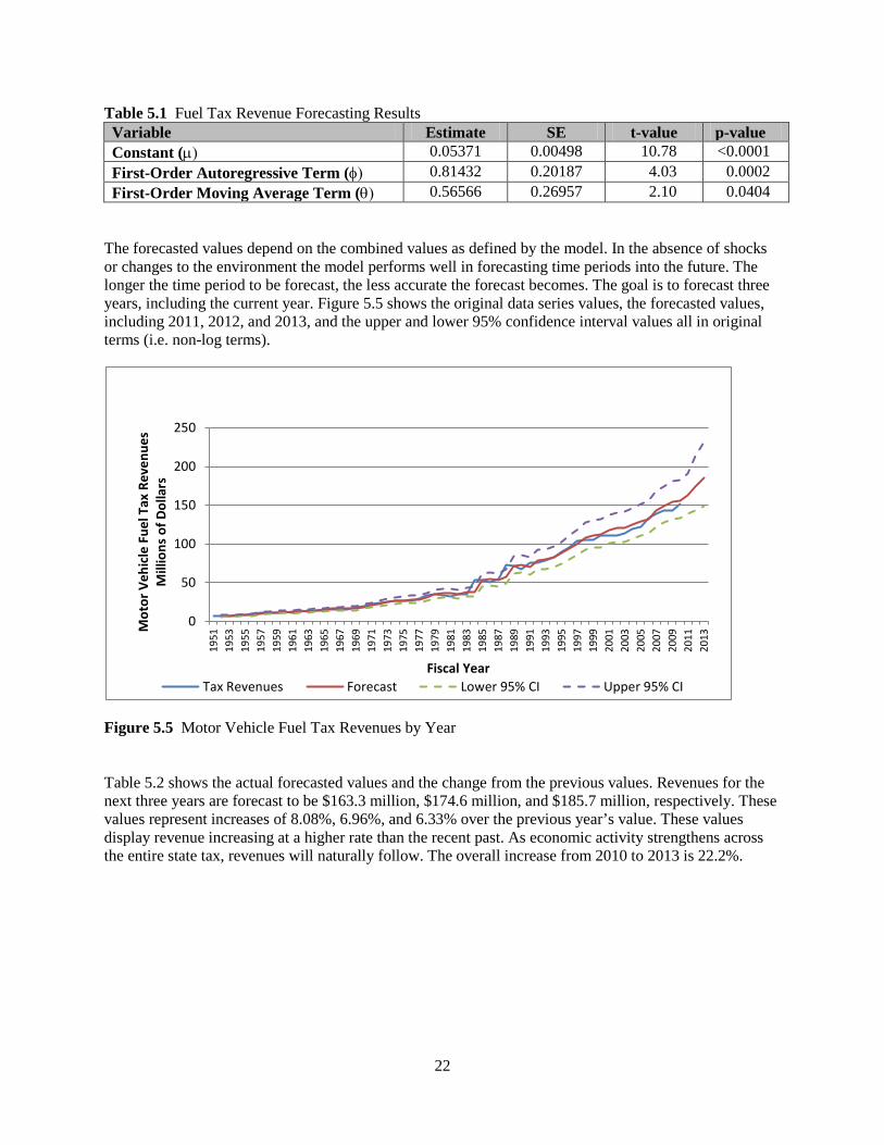
The forecasted values depend on the combined values as defined by the model. In the absence of shocks or changes to the environment the model performs well in forecasting time periods into the future. The longer the time period to be forecast, the less accurate the forecast becomes. The goal is to forecast three years, including the current year. Figure 5.5 shows the original data series values, the forecasted values, including 2011, 2012, and 2013, and the upper and lower 95% confidence interval values all in original terms (i.e. non-log terms).

Figure 5.5 Motor Vehicle Fuel Tax Revenues by Year Table 5.2 shows the actual forecasted values and the change from the previous values. Revenues for the next three years are forecast to be $163.3 million, $174.6 million, and $185.7 million, respectively. These values represent increases of 8.08%, 6.96%, and 6.33% over the previous year’s value. These values display revenue increasing at a higher rate than the recent past. As economic activity strengthens across the entire state tax, revenues will naturally follow. The overall increase from 2010 to 2013 is 22.2%.

0

50

100

150

200

250

1951

1953

1955

1957

1959

1961

1963

1965

1967

1969

1971

1973

1975

1977

1979

1981

1983

1985

1987

1989

1991

1993

1995

1997

1999

2001

2003

2005

2007

2009

2011

2013

Mot

or V

ehic

le F

uel T

ax R

even

ues

Mill

ions

of D

olla

rs

Fiscal Year Tax Revenues Forecast Lower 95% CI Upper 95% CI

23

Table 5.2 Actual and Forecast Values with Confidence Interval Year Actual Value Forecast Lower 95% CI Upper 95% CI % Change 2008 $143,389,000 $148,958,000 $127,117,000 $174,553,000 3.30% 2009 $143,796,000 $154,202,000 $131,592,000 $180,698,000 0.28% 2010 $151,050,000 $156,057,000 $133,175,000 $182,872,000 5.04% 2011 . $163,259,000 $139,320,000 $191,310,000 8.08%* 2012 . $174,623,000 $143,209,000 $212,929,000 6.96%* 2013 . $185,680,000 $148,907,000 $231,534,000 6.33%*

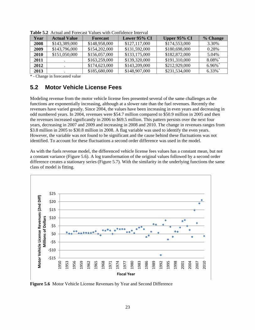
* - Change in forecasted value 5.2 Motor Vehicle License Fees Modeling revenue from the motor vehicle license fees presented several of the same challenges as the functions are exponentially increasing, although at a slower rate than the fuel revenues. Recently the revenues have varied greatly. Since 2004, the values have been increasing in even years and decreasing in odd numbered years. In 2004, revenues were $54.7 million compared to $50.9 million in 2005 and then the revenues increased significantly in 2006 to $69.5 million. This pattern persists over the next four years, decreasing in 2007 and 2009 and increasing in 2008 and 2010. The change in revenues ranges from $3.8 million in 2005 to $30.8 million in 2008. A flag variable was used to identify the even years. However, the variable was not found to be significant and the cause behind these fluctuations was not identified. To account for these fluctuations a second order difference was used in the model. As with the fuels revenue model, the differenced vehicle license fees values has a constant mean, but not a constant variance (Figure 5.6). A log transformation of the original values followed by a second order difference creates a stationary series (Figure 5.7). With the similarity in the underlying functions the same class of model is fitting.

Figure 5.6 Motor Vehicle License Revenues by Year and Second Difference

-$15

-$10

-$5

$0

$5

$10

$15

$20

$25

1950

1953

1956

1959

1962

1965

1968

1971

1974

1977

1980

1983

1986

1989

1992

1995

1998

2001

2004

2007

2010

Mot

or V

ehic

le L

icen

se R

even

ues (

2nd

Diff)

M

illio

ns o

f Dol

lars

Fiscal Year

24

Figure 5.7 Log of Motor Vehicle License Revenues by Year and Second Difference Fitting an ARIMA (1,2,1) model which indicates that there is both a first-order autoregressive term and a first-order moving average term with second order differencing of the logged values. Using the back-step notation yields the following conceptual model:

(1 − B)2Yt = µ + (1−θ1B)(1−ϕ1B)

at , where

t = Time period

Yt = Loge (motor vehicle fuel revenue) at time period t

µ = Constant term θ = First-order moving average term φ = First-order autoregressive term at= Random error at time period t

The estimates for the model are found in Table 5.3. Again the parameters are all highly significant and contribute to the predictive ability of the model. Table 5.3 Model Estimates for Vehicle Registration and License Fees

Variable Estimate SE t-value p-value Constant 0.09187 0.01611 5.70 <0.0001 First-Order Autoregressive Term -0.99755 0.02702 -36.93 <0.0001 First-Order Moving Average Term -0.69369 0.10723 -6.47 <0.0001

-0.1

0.0

0.1

0.2

0.3

0.4

0.5

1950

1953

1956

1959

1962

1965

1968

1971

1974

1977

1980

1983

1986

1989

1992

1995

1998

2001

2004

2007

2010

Log

of M

otor

Veh

icle

Lic

ense

Rev

enue

s (2

nd D

iffer

ence

)

Fiscal Year

25

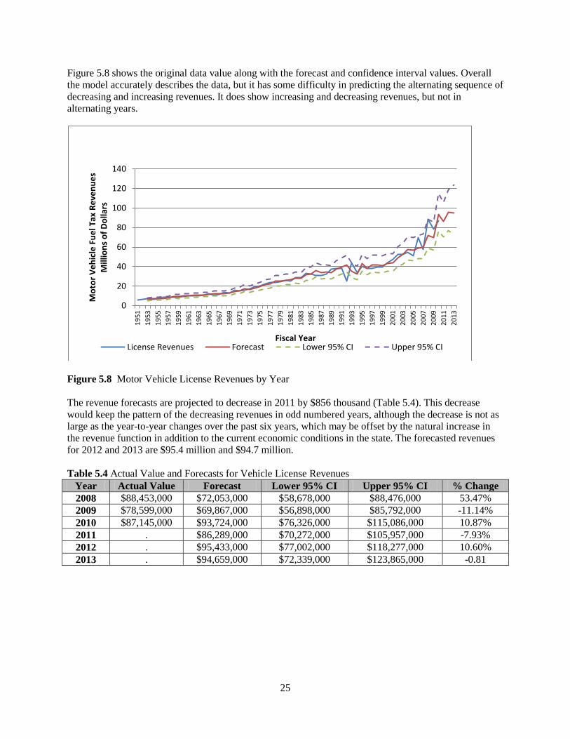
Figure 5.8 shows the original data value along with the forecast and confidence interval values. Overall the model accurately describes the data, but it has some difficulty in predicting the alternating sequence of decreasing and increasing revenues. It does show increasing and decreasing revenues, but not in alternating years.

Figure 5.8 Motor Vehicle License Revenues by Year The revenue forecasts are projected to decrease in 2011 by $856 thousand (Table 5.4). This decrease would keep the pattern of the decreasing revenues in odd numbered years, although the decrease is not as large as the year-to-year changes over the past six years, which may be offset by the natural increase in the revenue function in addition to the current economic conditions in the state. The forecasted revenues for 2012 and 2013 are $95.4 million and $94.7 million. Table 5.4 Actual Value and Forecasts for Vehicle License Revenues

Year Actual Value Forecast Lower 95% CI Upper 95% CI % Change 2008 $88,453,000 $72,053,000 $58,678,000 $88,476,000 53.47% 2009 $78,599,000 $69,867,000 $56,898,000 $85,792,000 -11.14% 2010 $87,145,000 $93,724,000 $76,326,000 $115,086,000 10.87% 2011 . $86,289,000 $70,272,000 $105,957,000 -7.93% 2012 . $95,433,000 $77,002,000 $118,277,000 10.60% 2013 . $94,659,000 $72,339,000 $123,865,000 -0.81

0

20

40

60

80

100

120

140

1951

1953

1955

1957

1959

1961

1963

1965

1967

1969

1971

1973

1975

1977

1979

1981

1983

1985

1987

1989

1991

1993

1995

1997

1999

2001

2003

2005

2007

2009

2011

2013

Mot

or V

ehic

le F

uel T

ax R

even

ues

Mill

ions

of D

olla

rs

Fiscal Year License Revenues Forecast Lower 95% CI Upper 95% CI

26

5.3 Conclusion Both models fit their respective data quite well. The forecasts in both cases seem plausible given the recent history and the current economic activity in North Dakota. For 2011, the motor vehicle fuel revenue is estimated to be $163,259,000 and the motor vehicle license revenue is estimated to be $86,289,000. This gives the state total revenues of just under $250 million, an increase of 4.8% over 2010. Continued oil activity in western North Dakota may push these numbers higher as economic activity continues to increase. Increases in population should result in more vehicles in North Dakota and higher revenue in both motor fuels tax revenue and vehicle license and registration fees. Revenues will likely increase from both the gasoline tax and the diesel tax, which may grow at different rates. This fact may require separate models be built to accurately describe the two revenue streams and forecast future overall revenues. The stated forecasts are short term in nature and need to be continually updated. Even though the regressor variables investigated in this model-building work were not found to be statistically significant, additional work with these and other import economic variables may prove fruitful in light of other states’ findings. It may be that these variables associated with the overall economy in North Dakota are not important for several reasons even though some other states find varying degrees of significance for them. In fact, some states find significance for quarterly estimate models, but not annual models. Many of these states also have more of a manufacturing base where North Dakota, with the exception of the last few years, has been predominately agricultural. The overall economy and the agricultural economy are not always in lock step. At times the overall economy may be slow, but the agricultural economy remains strong or the overall economy is strong but depressed farm prices push the agricultural economy down. This type of “dual” economy scenario often shields North Dakota from deep recessions. Many other factors contribute to changes in the amount of revenues collected from both the motor vehicle fuel tax and the motor vehicle license fees. Fuel tax revenues can be affected by federal government requirements to raise the average fuel economy of each manufacturer’s fleet of vehicles, gas and diesel prices, changes in the farm truck fleet, and development of alternative fuels, (specifically electric or hydrogen fuel cell vehicles). The size of the population, the economy, license fees, etc. may all affect how many vehicles a family, business, or farming operation own and license. Changes in government policy in reaction to any of these changes may lag the actual changes by several years. The current model estimates needs to be evaluated against actual outcomes to assess the models ability to accurately predict the revenue streams. These assessments will indicate whether there is a need to build new models or more complex models due to low reliability of the current models and to account for any changes in the system.

27

6. SUMMARY The literature reveals that most states forecast revenues using either statistical or econometric models. These models provide states with valuable information for budgeting and meeting or setting their obligation authority. States use different approaches. While forecasting for fuel revenue, some states estimate VMT and fuel efficiency of the fleet and the fleet disposition. Other states use historical and other variables such as GSP, income, employment etc. as variables for the forecasting models. Most models have evolved over time and states are focusing on continuous improvement in their forecasting models that can provide them with the best results during economic growth or recession. Gillen provided insight in the 1990s into the problems with states’ forecasts of fuel revenue. Some states have employed his approach. One approach is to use experts or consensus forecasts to at least set the parameters of the forecast in the face of economic or political or social changes. Others states use more complex modeling and are forecasting more frequently in an attempt to increase accuracy. The survey of the 50 states had a 20% response rate. The survey found that 80% reported forecasting for motor fuels tax revenues. Linear regression is the most popular technique being used by half of the respondents. Two states reported using consensus estimates for setting the dependent and independent variables. One state reports using only consensus forecasting. Three states use a simple trend analysis while one state reports using only historical data to estimate future revenues while the other reports using an auto regressive model to create confidence intervals. Forty percent of the states forecast annually, half forecast semiannually, 20% report quarterly and one reports a monthly forecast. The highest forecast error was almost 9% and the weighted average of the largest forecast error was 3.5%. External variables are used by 60% of respondents while 40% responded they do not use an external variable. Only 40% of states use fuel price as a predictor of motor fuels tax revenue collections and only one uses gross state product (GSP). Respondents reported the years with the largest forecast errors. The reason for this question was to try to determine if the model was resilient to shocks to the economy. The respondents were asked to pick the three years with the highest forecast errors. The years with the largest forecast errors were 2008 and 2009 with 60% and 50% respectively. The country was in economic recession in 2008 and 2009. The collapse of the housing industry and resulting distress in the financial sector made economic forecasting difficult. The survey revealed that 80% of the states responding use a forecasting model to estimate license and registration fees. Half of the states stratify the forecasts by vehicle type. Linear regression is reported as the forecasting model used by 50% of the states reporting to estimate motor vehicle licenses and registration fees. Thirty percent of respondents conduct forecasts semi-annually and another 30% report they forecast annually. Twenty percent forecast quarterly and only one state forecasts on a monthly basis. Forecasting accuracy may be more difficult than forecasting motor fuel tax revenue, as 60% reported forecast errors of greater than 7% for motor vehicle licenses and registration fees. Arizona commented that its highest error for this category was 14.9% in 2008. The highest errors in forecasting occurred in 2007, 2008, and 2009 were picked by 40% of the states with 2010 picked by 30% of states. The most common error in forecasting vehicle licenses and registration revenues was between 2% and 3% with 25% reporting less than 1% error in forecasting. Both models fit their respective data quite well. The forecasts in both cases seem plausible given the recent history and the current economic activity in North Dakota. For 2011, motor vehicle fuel revenue is estimated to be $163,259,000 and the motor vehicle license revenue is estimated to be $86,289,000. This

28

gives the state total revenues of just under $250 million, an increase of 4.8% over 2010. Continued oil activity in western North Dakota may push these numbers higher as economic activity continues to increase. Increases in population should result in more vehicles in North Dakota and higher revenue in both motor fuels tax revenue and vehicle license and registration fees. Revenues will likely increase from both the gasoline tax and the diesel tax, which may grow at different rates. This fact may require separate models be built to accurately describe the two revenue streams and forecast future overall revenues. The stated forecasts are short term in nature and need to be continually updated. Even though the regressor variables investigated in this model-building work were not found to be statistically significant, additional work with these and other import economic variables may prove fruitful in light of other states’ findings. It may be that these variables associated with the overall economy in ND are not important for several reasons even though some other states find varying degrees of significance for them. In fact some states find significance for quarterly estimate models, but not annual models. Many of these states also have more of a manufacturing base while North Dakota, with the exception of the last few years, has been predominately agricultural. The overall economy and the agricultural economy are not always in lock step. At times the overall economy may be slow, but the agricultural economy remains strong or the overall economy is strong but depressed farm prices push the agricultural economy down. This type of “dual” economy scenario often shields North Dakota from deep recessions. Many other factors contribute to changes in the amount of revenues collected from both the motor vehicle fuel tax and the motor vehicle license fees. Fuel tax revenues can be affected by federal government requirements to raise the average fuel economy of each manufacturer’s fleet of vehicles, gas and diesel prices, changes in the farm truck fleet, and development of alternative fuels (specifically electric or hydrogen fuel cell vehicles). The size of the population, the economy, license fees, etc. may all affect how many vehicles a family, business, or farming operation own and license. Changes in government policy in reaction to any of these changes may lag the actual changes by several years. The current model estimates needs to be evaluated against actual outcomes to assess the models ability to accurately predict the revenue streams. These assessments will indicate whether there is a need to build new models or more complex models due to low reliability of the current models and to account for any changes in the system.

29

REFERENCES 1. Arizona Department of Transportation. Update of the Highway User Revenue Fund and

Maricopa Regional Area Road Fund Forecasting Models, prepared by HDR|HLB Decision Economics Inc. July 2005.

2. Box, George and Gwilym Jenkins. 1976. Time Series Analysis: Forecasting and Control. Holden-Day Oakland, CA.

3. Bureau of Economic Analysis 2009. Gross Domestic Product by State. Accessed online March 28, 2011 at http://www.bea.gov/regional/gsp/.

4. California Department of Transportation. California Motor Vehicle Stock, Travel and Fuel Forecast. December 2006.

5. Department of Mineral Resources, Oil and Gas Division. 2011. General Statistics. North Dakota Industrial Commission. Accessed online March 28, 2011 at https://www.dmr.nd.gov/oilgas/.

6. HDR/HLB Decision Economics Inc., 2010. Review and Critique MODOT’s State Revenue Forecasting Model. Final Report. Silver Spring, MD.

7. HDR|HLB Decision Economics, Inc. 2007. Review and Critique MODOT’s State Revenue Forecasting Model. Silver Spring, MD.

8. Gillen, David. “Estimating Revenues from User Charges Taxes and Fees: Identifying Information Requirements.” Transportation Research Board Conference Proceedings 21. 2000.

9. Kouris, G. “Fuel Consumption for Road Transport in the U.S.A.” Energy Economics, 5(2), 1983.

10. Shinn, Paul. 2010. State Revenue Forecasting Project 2010 Technical Memorandum. Oklahoma Policy Institute. Tulsa, OK.

11. United States Census Bureau. 2010. Population Estimates, accessed online March 28, 2011 at http://www.census.gov/popest/states/states.html.

12. United States Census Bureau. 2010. Annual Survey of State Government Tax Collections, accessed online March 28, 2011 at http://www.census.gov/govs/statetax/.

13. U.S. Energy Information Administration. 2010

14. Washington State Department of Transportation – Economic Analysis, 2010. Statewide Fuel

Consumption Forecast Models. Washington State Department of Transportation. Olympia, WA.

15. Washington State Department of Transportation. Statewide Fuel Consumption Forecast Models 2010.

16. Varma, A., K.C. Sinha, and J.L. Spalding. The Development of A Highway Revenue Forecasting Model for Indiana. Joint Highway Research Project. Purdue University, 1992.

30

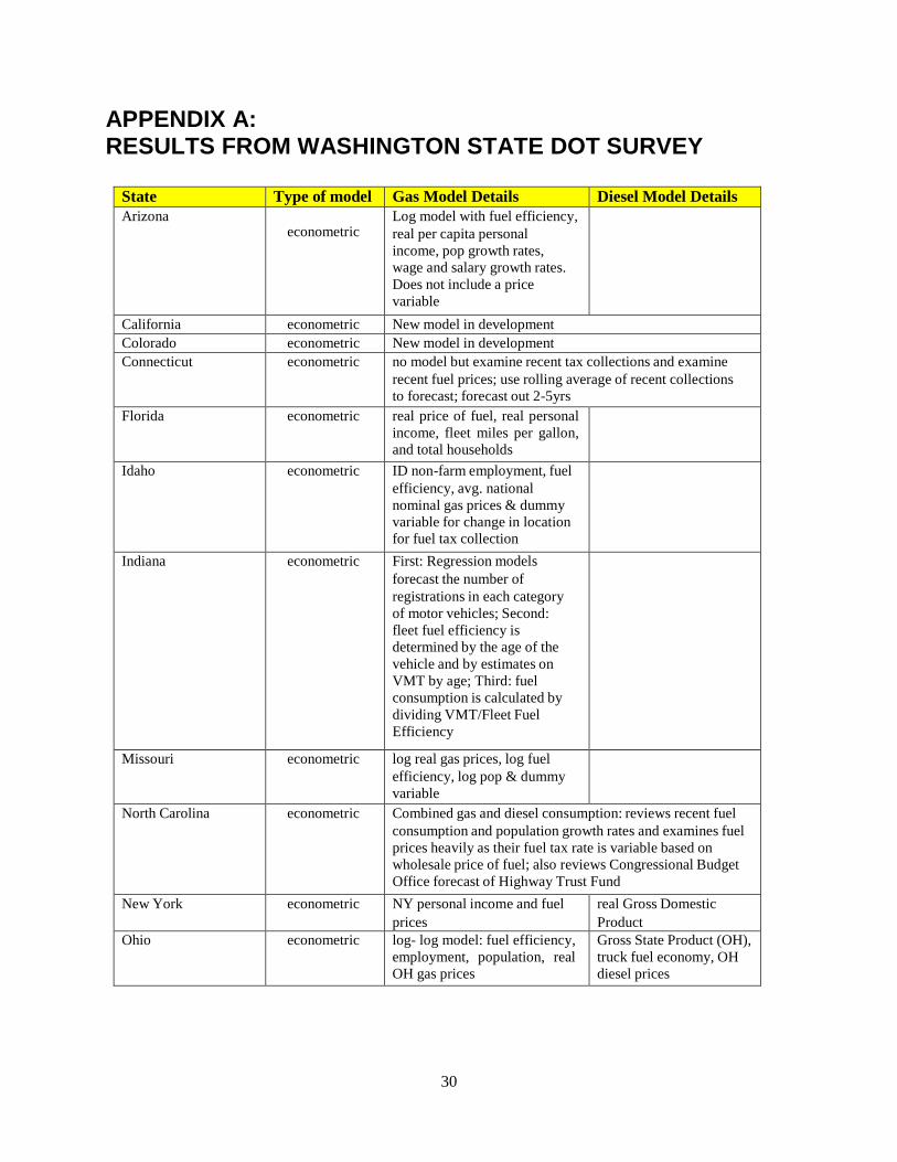
APPENDIX A: RESULTS FROM WASHINGTON STATE DOT SURVEY

State Type of model Gas Model Details Diesel Model Details Arizona

econometric Log model with fuel efficiency, real per capita personal income, pop growth rates, wage and salary growth rates. Does not include a price variable

California econometric New model in development Colorado econometric New model in development Connecticut econometric no model but examine recent tax collections and examine

recent fuel prices; use rolling average of recent collections to forecast; forecast out 2-5yrs

Florida econometric real price of fuel, real personal income, fleet miles per gallon, and total households

Idaho econometric ID non-farm employment, fuel efficiency, avg. national nominal gas prices & dummy variable for change in location for fuel tax collection

Indiana econometric First: Regression models forecast the number of registrations in each category of motor vehicles; Second: fleet fuel efficiency is determined by the age of the vehicle and by estimates on VMT by age; Third: fuel consumption is calculated by dividing VMT/Fleet Fuel Efficiency

Missouri econometric log real gas prices, log fuel efficiency, log pop & dummy variable

North Carolina econometric Combined gas and diesel consumption: reviews recent fuel consumption and population growth rates and examines fuel prices heavily as their fuel tax rate is variable based on wholesale price of fuel; also reviews Congressional Budget Office forecast of Highway Trust Fund

New York econometric NY personal income and fuel prices

real Gross Domestic Product

Ohio econometric log- log model: fuel efficiency, employment, population, real OH gas prices

Gross State Product (OH), truck fuel economy, OH diesel prices

31

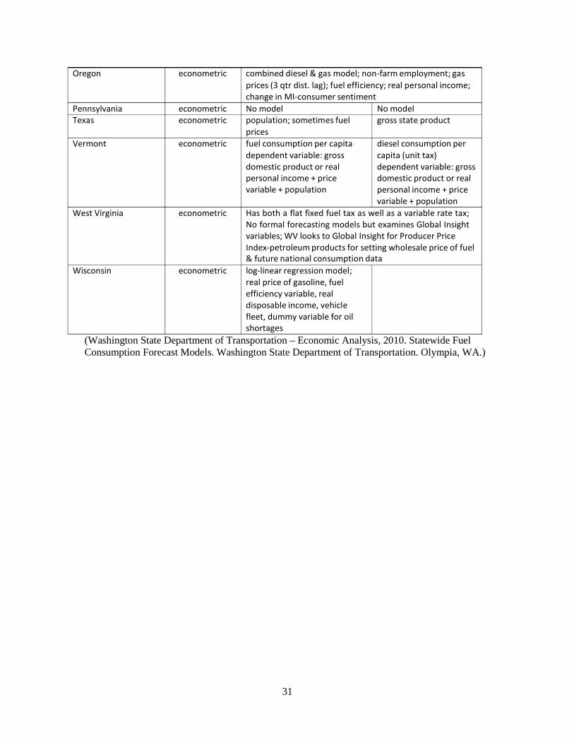
(Washington State Department of Transportation – Economic Analysis, 2010. Statewide Fuel Consumption Forecast Models. Washington State Department of Transportation. Olympia, WA.)

Oregon econometric combined diesel & gas model; non-farm employment; gas prices (3 qtr dist. lag); fuel efficiency; real personal income; change in MI-consumer sentiment

Pennsylvania econometric No model No model Texas econometric population; sometimes fuel

prices gross state product

Vermont econometric fuel consumption per capita dependent variable: gross domestic product or real personal income + price variable + population

diesel consumption per capita (unit tax) dependent variable: gross domestic product or real personal income + price variable + population

West Virginia econometric Has both a flat fixed fuel tax as well as a variable rate tax; No formal forecasting models but examines Global Insight variables; WV looks to Global Insight for Producer Price Index-petroleum products for setting wholesale price of fuel & future national consumption data

Wisconsin econometric log-linear regression model; real price of gasoline, fuel efficiency variable, real disposable income, vehicle fleet, dummy variable for oil shortages

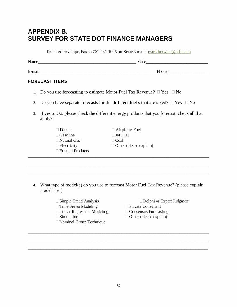
32

APPENDIX B. SURVEY FOR STATE DOT FINANCE MANAGERS

Enclosed envelope, Fax to 701-231-1945, or Scan/E-mail: mark.berwick@ndsu.edu

Name______________________________________________ State_____________________________ E-mail_______________________________________________________Phone: __________________ FORECAST ITEMS

1. Do you use forecasting to estimate Motor Fuel Tax Revenue? � Yes � No

2. Do you have separate forecasts for the different fuel s that are taxed? � Yes � No

3. If yes to Q2, please check the different energy products that you forecast; check all that apply?

� Diesel � Airplane Fuel � Gasoline � Jet Fuel � Natural Gas � Coal � Electricity � Other (please explain) � Ethanol Products

_____________________________________________________________________________________ ____________________________________________________________________________________________________________________ ____________________________________________________________________________________________________________________

4. What type of model(s) do you use to forecast Motor Fuel Tax Revenue? (please explain model i.e. )

� Simple Trend Analysis � Delphi or Expert Judgment � Time Series Modeling � Private Consultant � Linear Regression Modeling � Consensus Forecasting � Simulation � Other (please explain) � Nominal Group Technique

_____________________________________________________________________________________ ____________________________________________________________________________________________________________________ ____________________________________________________________________________________________________________________

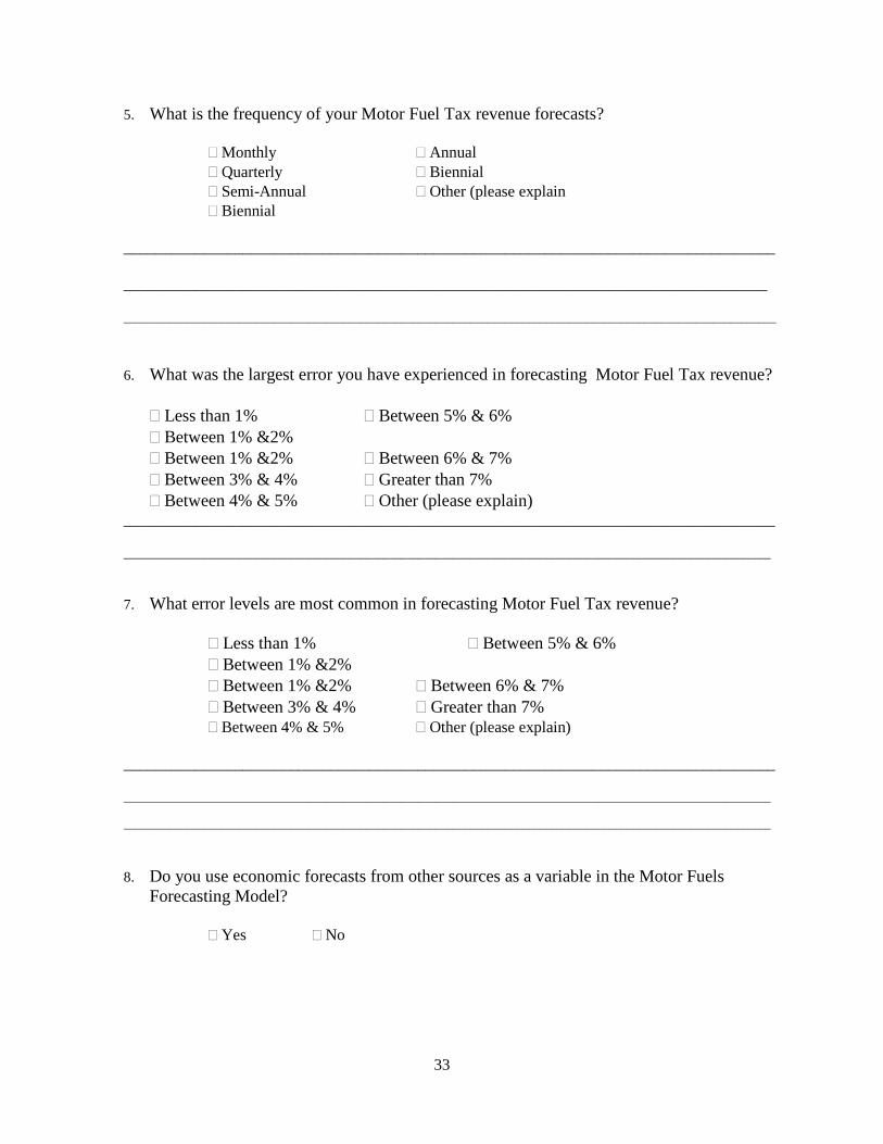
33

5. What is the frequency of your Motor Fuel Tax revenue forecasts?

� Monthly � Annual � Quarterly � Biennial � Semi-Annual � Other (please explain � Biennial

__________________________________________________________________________________ _________________________________________________________________________________ _________________________________________________________________________________________________________________

6. What was the largest error you have experienced in forecasting Motor Fuel Tax revenue? � Less than 1% � Between 5% & 6% � Between 1% &2% � Between 1% &2% � Between 6% & 7% � Between 3% & 4% � Greater than 7% � Between 4% & 5% � Other (please explain)

__________________________________________________________________________________ ________________________________________________________________________________________________________________

7. What error levels are most common in forecasting Motor Fuel Tax revenue?

� Less than 1% � Between 5% & 6% � Between 1% &2% � Between 1% &2% � Between 6% & 7% � Between 3% & 4% � Greater than 7% � Between 4% & 5% � Other (please explain)

__________________________________________________________________________________ ________________________________________________________________________________________________________________ ________________________________________________________________________________________________________________

8. Do you use economic forecasts from other sources as a variable in the Motor Fuels Forecasting Model?

� Yes � No

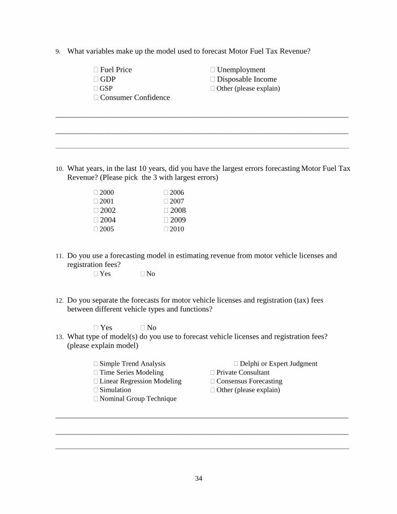
34

9. What variables make up the model used to forecast Motor Fuel Tax Revenue?

� Fuel Price � Unemployment � GDP � Disposable Income � GSP � Other (please explain) � Consumer Confidence

__________________________________________________________________________________ __________________________________________________________________________________ _________________________________________________________________________________________________________________

10. What years, in the last 10 years, did you have the largest errors forecasting Motor Fuel Tax Revenue? (Please pick the 3 with largest errors)

� 2000 � 2006

� 2001 � 2007

� 2002 � 2008 � 2004 � 2009 � 2005 � 2010

11. Do you use a forecasting model in estimating revenue from motor vehicle licenses and registration fees?

� Yes � No

12. Do you separate the forecasts for motor vehicle licenses and registration (tax) fees between different vehicle types and functions?

� Yes � No 13. What type of model(s) do you use to forecast vehicle licenses and registration fees?

(please explain model)

� Simple Trend Analysis � Delphi or Expert Judgment � Time Series Modeling � Private Consultant � Linear Regression Modeling � Consensus Forecasting � Simulation � Other (please explain) � Nominal Group Technique

__________________________________________________________________________________ __________________________________________________________________________________ _________________________________________________________________________________________________________________

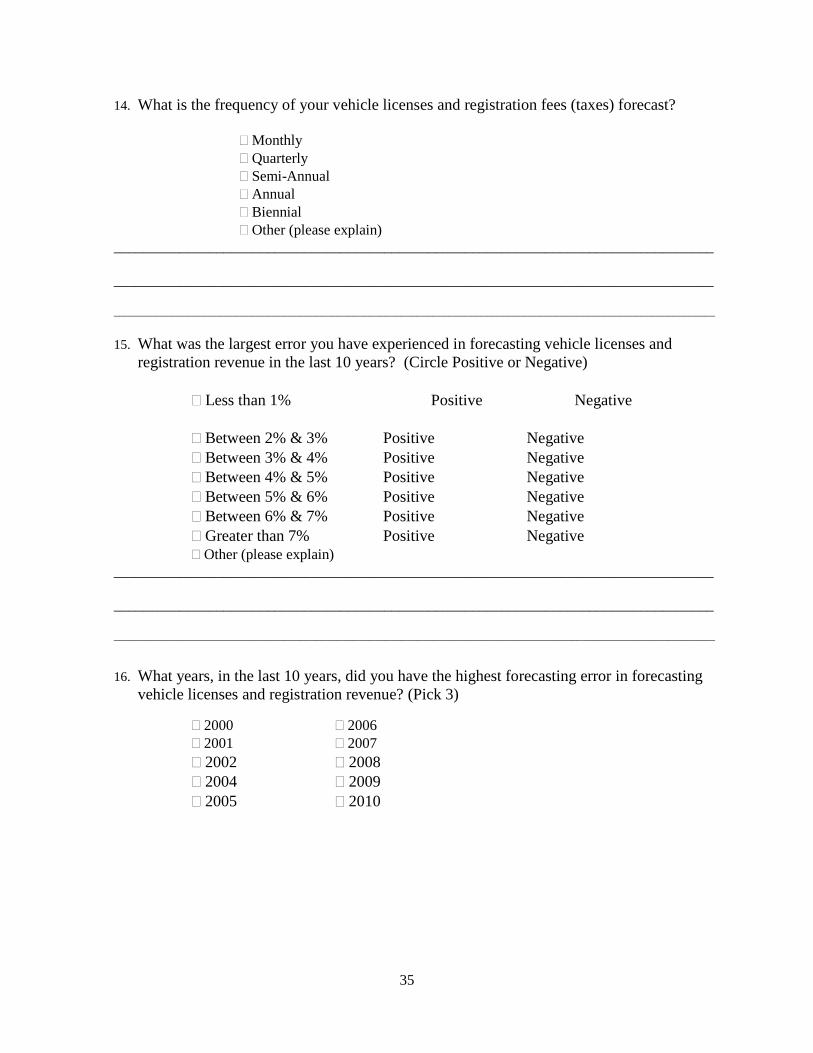
35

14. What is the frequency of your vehicle licenses and registration fees (taxes) forecast?

� Monthly � Quarterly � Semi-Annual � Annual � Biennial � Other (please explain)

__________________________________________________________________________________ __________________________________________________________________________________ _________________________________________________________________________________________________________________

15. What was the largest error you have experienced in forecasting vehicle licenses and

registration revenue in the last 10 years? (Circle Positive or Negative) � Less than 1% Positive Negative � Between 2% & 3% Positive Negative � Between 3% & 4% Positive Negative � Between 4% & 5% Positive Negative � Between 5% & 6% Positive Negative � Between 6% & 7% Positive Negative � Greater than 7% Positive Negative � Other (please explain)

__________________________________________________________________________________ __________________________________________________________________________________ _________________________________________________________________________________________________________________

16. What years, in the last 10 years, did you have the highest forecasting error in forecasting

vehicle licenses and registration revenue? (Pick 3)

� 2000 � 2006

� 2001 � 2007

� 2002 � 2008 � 2004 � 2009 � 2005 � 2010

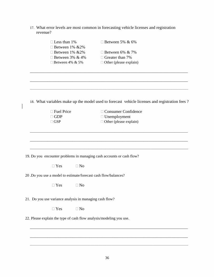
36

17. What error levels are most common in forecasting vehicle licenses and registration revenue?

� Less than 1% � Between 5% & 6% � Between 1% &2% � Between 1% &2% � Between 6% & 7% � Between 3% & 4% � Greater than 7% � Between 4% & 5% � Other (please explain)

__________________________________________________________________________________ __________________________________________________________________________________ _________________________________________________________________________________________________________________

18. What variables make up the model used to forecast vehicle licenses and registration fees ?

� Fuel Price � Consumer Confidence � GDP � Unemployment � GSP � Other (please explain)

__________________________________________________________________________________ __________________________________________________________________________________ _________________________________________________________________________________________________________________

19. Do you encounter problems in managing cash accounts or cash flow?

� Yes � No

20 .Do you use a model to estimate/forecast cash flow/balances?

� Yes � No

21. Do you use variance analysis in managing cash flow?

� Yes � No

22. Please explain the type of cash flow analysis/modeling you use.

__________________________________________________________________________________ __________________________________________________________________________________ _________________________________________________________________________________________________________________

37

23. How many different cash balances are you estimating and what are their purposes? (please explain)

Number_________ Purposes_______________________________________________________________________________________

__________________________________________________________________________________ __________________________________________________________________________________ _________________________________________________________________________________________________________________

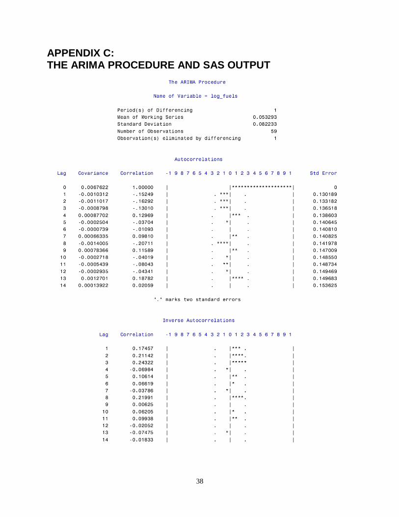
38

APPENDIX C: THE ARIMA PROCEDURE AND SAS OUTPUT

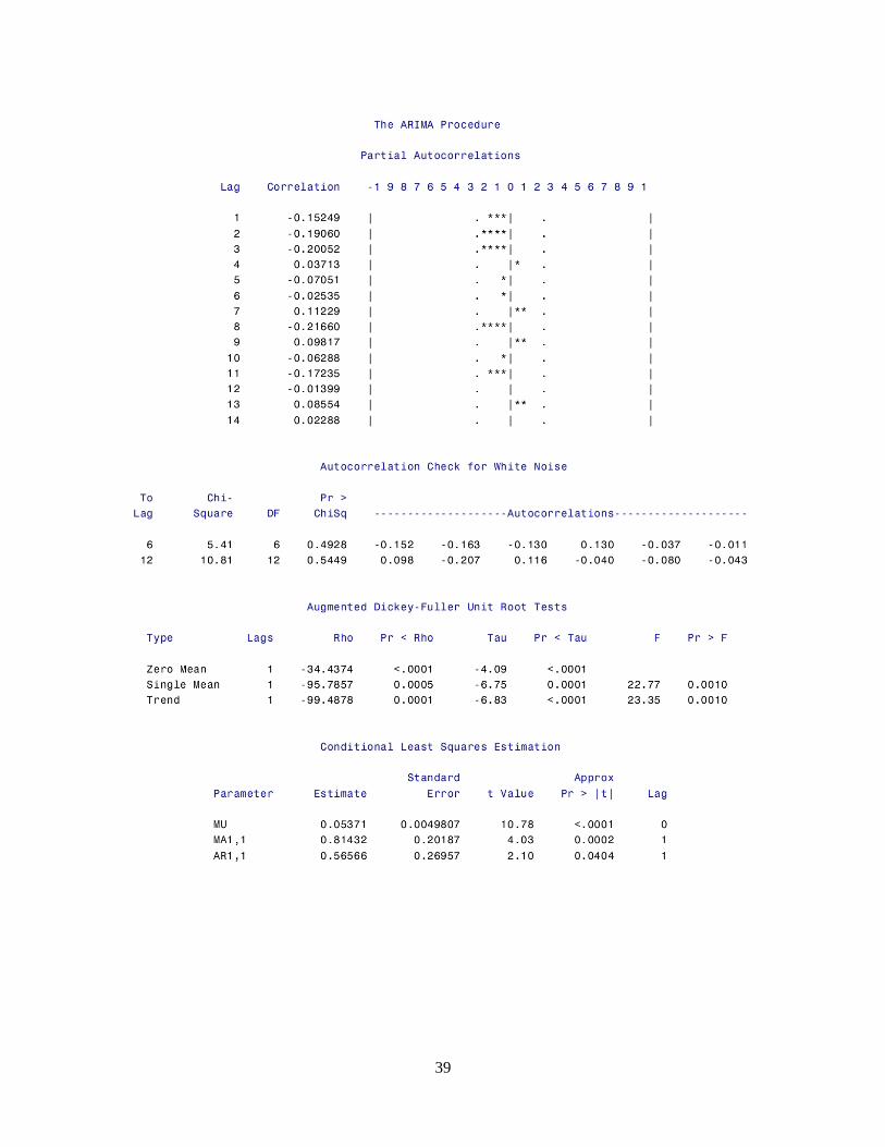
39

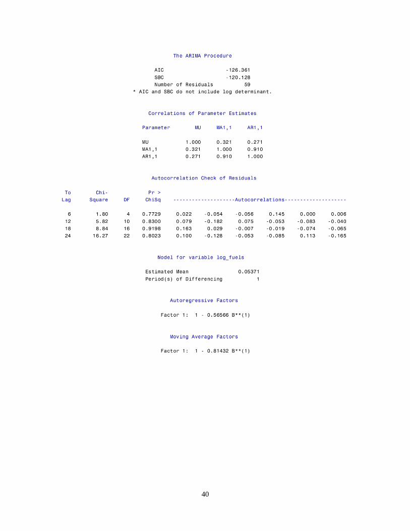
40

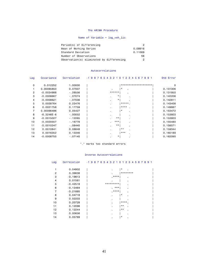
41

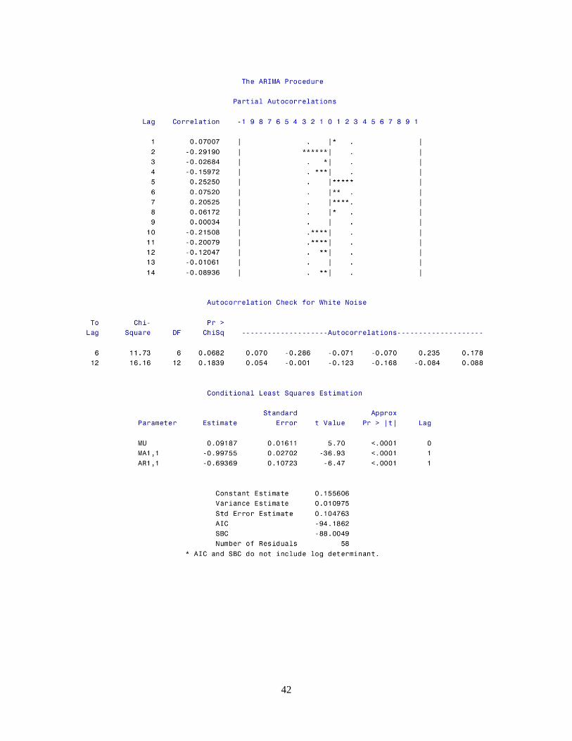
42

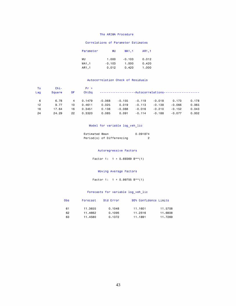
43