forecasting stock price with the residual income … forecasting stock price with the residual...
TRANSCRIPT

1
Forecasting Stock Price with the Residual Income Model
Huong N. Higgins. Worcester Polytechnic Institute Department of Management
100 Institute Road Worcester, MA 01609 Tel: (508) 831-5626 Fax: (508) 831-5720
Email: [email protected]
2
Forecasting Stock Price with the Residual Income Model
Abstract
This paper demonstrates a method to forecast stock price using analyst earnings forecasts as
essential signals of firm valuation. The demonstrated method is based on the Residual Income Model
(RIM), with adjustment for autocorrelation. Over the past decade, the RIM is widely accepted as a
theoretical framework for equity valuation based on fundamental information from financial reports.
This paper shows how to implement the RIM for forecasting, and how to address autocorrelation to
improve forecast accuracy. Overall, this paper provides a method to forecast stock price that blends
fundamental data with mechanical analyses of past time series.
3
Forecasting Stock Price with the Residual Income Model
Introduction
This paper demonstrates a method to forecast stock price using analyst earnings forecasts as
essential signals of firm valuation. The demonstrated method is based on the Residual Income Model
(RIM), a widely used theoretical framework for equity valuation based on accounting data. Despite its
importance and wide acceptance, the RIM yields large errors when applied for forecasting. This paper
discusses a statistical approach to improve stock price forecasts based on the RIM, specifically by
showing that adjusting for serial correlation in the RIM’s model (autocorrelation) yields more
accurate price forecasts. The demonstrated approach complements other valuation techniques, as
employing a basket of valid techniques builds confidence in pricing. Accurate price forecasts help
build a profitable trading strategy, for example by investing in stocks with the largest difference
between current price and forecast future price. In practice, although fundamentalists rely on true
economic strengths of the firm for valuation, there is ample room for mechanical analyses of price
trends. This paper serves investment professionals by providing a pricing method that blends
fundamental information in analyst earnings forecasts with mechanical analyses of time series.
The RIM is a theoretical model which links stock price to book value, earnings in excess of a
normal capital charge (abnormal earnings), and other information ( tv ). Other information tv can be
interpreted as capturing value-relevant information about the firm’s intangibles, which are poorly
measured by financial reported numbers. This interpretation recognizes that a portion of valuation
stems from factors not to be captured in financial statements. Other information tv can also be
interpreted as capturing different sorts of errors and noises, including model mis-specification,
measurement error, serial correlation, and white noise. Given the possible imperfections of any
valuation model, the content of tv is elusive and it is the purpose of this paper to exploit it to the best
using statistical tools to predict stock price. To the extent that tv contains serial correlation, as

4
expected in firm data, modeling its time series properties should improve the forecasting performance
of the RIM.
First, I demonstrate how to implement the RIM using one term of abnormal earnings. I
review the theoretical framework, and model the RIM to parallel forecasters’ task just before time t to
forecast stock price at time t based on expected earnings for the period ending at t. The forecaster’s
information at the time of the task consists of book value at the beginning of the period ( 1−tbv ),
expected earnings of the current period ( tx , for the period staring at t-1 and ending at t), and the
normal capital charge rate for the period ( tr ). Abnormal earning is defined as the difference between
analyst earnings forecast (best knowledge of actual earnings) and the earnings number achieved under
growth of book value at a normal discount rate. Underlying this definition is the idea that analyst
earnings forecasts are essential signals of firm valuation (following Frankel and Lee 1998, Francis et
al. 2000, and Sougiannis and Yaekura 2001).
Next, I demonstrate how to improve the implementation of the RIM. I describe the necessary
procedures starting with a naïve regression. Then, I point out the violations of this naïve regression,
and seek improvement by addressing these violations. Specifically, for RIM regressions to produce
reliable results, tv must have a normal zero-mean distribution and meet the statistical regression
assumptions. However, the regression assumptions are often not met, due to strong serial correlation
in tv . Serial correlation arises when a variable is correlated with its own value from a different time
lag, and is a notorious problem in financial and economic data. This problem can be addressed by
using regressions with time series errors to model the properties of tv . My diagnostics also show
conditional heteroscedasticity in tv , which can be addressed with GARCH modeling. My procedure
to identify the time series properties of tv is as recommended by Tsay (2002) and Shumway and
Stoffer (2005). I show that, by jointly estimating the RIM regression and the time series models of tv ,
forecast errors are substantially reduced.

5
My demonstration is based on SP500 firms, using 22 years of data spanning 1982 – 2003 to
estimate the prediction models, which I then use to predict stock prices in a separate period spanning
2004 - 2005. The mean absolute percentage error obtained can be as low as 18.12% in one-year-ahead
forecasts, and 29.42% in two-year-ahead forecasts. It is important to note that I use out-of-sample
forecasts, whereas many prior studies use in-sample forecasting, in other words, they do not separate
the estimation period from the forecast period. In-sample forecasts have artificially lower forecast
error than out-of-sample because hindsight information is incorporated. However, to be of practical
value, forecasts must be done beyond the estimation baseline.
For a brief review of prior results, prior valuation studies based on the RIM have focused
more on determining value relevance, i.e., the contemporaneous association between stock price and
accounting variables, not to forecast future prices. As will be noted in this paper, the harmful effect of
autocorrelation is not apparent in estimation or tests of association, therefore value-relevance studies
may not have to address this issue. However, when the RIM results are applied for forecasting, it
yields large errors, although the RIM is found to produce more accurate forecasts than alternatives
such as the dividend discount model and the free cash flow model (Penman and Sougiannis 1998,
Francis et al. 2000). Forecast errors are disturbingly large, and valuations tend to understate stock
price (See discussions of large forecast errors in Choi et al. 2006, Sougiannis and Yaekura 2001,
Frankel and Lee 1998, DeChow et al. 1999, Myers 1999). The errors are larger with out-of-sample
forecasts, because the new observations to be forecasted are farther from the center of the estimation
sample. The large errors could be due to many factors, including inappropriate terminal values,
discount rates, and growth rate (Lundholm and O’Keefe 2001, Sougiannis and Yaekura 2001), and
autocorrelation as argued in this paper. This paper discusses how to address the autocorrelation factor
to improve RIM-based stock price forecasts.
The paper proceeds as follows. To demonstrate how to implement the RIM, Section 2
reviews the theoretical RIM, discusses its adaptations for empirical analyses, and describes its
implementation with one term of abnormal earnings. To demonstrate how to improve the

6
implementation of the RIM, Section 3 discusses the empirical data and diagnostics methods of tv to
identify its proper structures. Section 4 describes the results of estimating jointly the RIM regressions
and the time series structures of tv , and discusses the forecast results. Section 5 presents extension
analyses. Section 6 summarizes and concludes the paper.
2. The RIM
2.1. The Theoretical RIM
In economics and finance, the traditional approach to value a single firm is based on the
Dividend Discount Model (DDM), as described by Rubinstein (1976). This model defines the value
of a firm as the present value of its expected future dividends.
[ ]∑∞
=
+−+=
0
)1(k
kt
k
tt drP (1)
where Pt is stock price, tr is the discount rate, and dt is dividend at time t. Equation (1) relates cum-
dividend price at time t to an infinite series of discounted dividends where the series starts at time t.1
The idea of DDM implies that one should forecast dividends in order to estimate stock price.
The DDM has disadvantages because dividends are arbitrarily determined, and many firms do not pay
dividends. Moreover, market participants tend to focus on accounting information, especially
earnings.
Starting from the DDM, Peasnell (1982) links dividends to fundamental accounting
measurements such as book value of equity, and earnings:
1 Many prior RIM papers use ex-dividend price equations, the results of which carry through to relate price at time t to equity book value at time t and discounted abnormal earnings starting at time t+1. This paper’s Equation (1) uses cum-dividend price and carries through to relate price at time t to equity book value at time t-1 and discounted abnormal earnings at time t. This approach helps define abnormal earnings based on expected earnings of the contemporaneous period and therefore can aid the actual price forecast task. In other words, in linking price and contemporaneous abnormal earnings, this model parallels the forecaster’s decision in forecasting stock price at a certain point in period t (starting at t-1 and ending at t), when her information consists of book value at the beginning
of the year ( 1−tbv ), and earnings forecasts of the current year ( tx ).

7
tttt dxbvbv −+= −1 (2)
where tbv is book value at time t. Ohlson (1995) refers to Equation (2) as the Clean Surplus Relation.
From Equation (2), dividends can be formulated in terms of book values and earnings:
)( 1−−−= tttt bvbvxd (3)
Define a
tx = 1−− ttt bvrx , termed “abnormal earnings’, to denote earnings minus a charge
for the use of capital. (4) From (3) and (4):
1*)1( −++−= ttt
a
tt bvrbvxd (5)
Rewriting Equation (1):
......][)1(
1][
)1(
1][
1
1][ 33221 +
++
++
++= +++ t
t
t
t
t
t
tt dr
dr
dr
dP
Using (5) to replace 21
,,++ ttt ddd … , in Equation (1) yields:
∑∞
=
+−
− ++=0
1 ][)1(k
a
kt
k
ttt xrbvP (6),
provided that 0)1(→
+
+
n
t
nt
r
bν. As in Ohlson (1995), this provision is assumed satisfied.
I refer to Equation 6 as the theoretical RIM, which equates firm value to the previous book
value and the present value of firm current and future abnormal earnings.2
2.2. Adapting the Theoretical RIM for Empirical Analyses – RIM Regression
In practice, it is impossible to work with an infinite stream of residual incomes as in Equation
(6), and approximations over finite ad-hoc horizons are necessary. Consider an adaptation that
purports to capture value over a finite horizon:
t
n
k
a
kt
k
ttt xrbvP ν+++= ∑=
+−
−
0
1 ][)1( (7)
2 This development of the theoretical RIM follows the steps described by Ohlson (1995), except that Ohlson (1995) uses ex-dividend price.
8
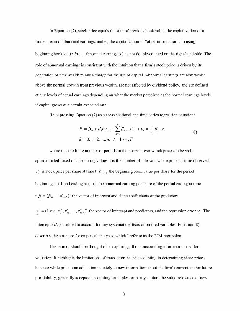
In Equation (7), stock price equals the sum of previous book value, the capitalization of a
finite stream of abnormal earnings, and tv , the capitalization of “other information”. In using
beginning book value 1−tbv , abnormal earnings a
tx is not double-counted on the right-hand-side. The
role of abnormal earnings is consistent with the intuition that a firm’s stock price is driven by its
generation of new wealth minus a charge for the use of capital. Abnormal earnings are new wealth
above the normal growth from previous wealth, are not affected by dividend policy, and are defined
at any levels of actual earnings depending on what the market perceives as the normal earnings levels
if capital grows at a certain expected rate.
Re-expressing Equation (7) as a cross-sectional and time-series regression equation:
. , ,1 ;...,21,0
~
'
~0
2110
Ttn, , k
vxvxbvP tt
t
n
k
a
ktktt
L==
+=+++= ∑=
++− ββββ (8)
where n is the finite number of periods in the horizon over which price can be well
approximated based on accounting values, t is the number of intervals where price data are observed,
tP is stock price per share at time t, 1−tbv the beginning book value per share for the period
beginning at t-1 and ending at t, a
tx the abnormal earning per share of the period ending at time
t, )',( 20~
+= nβββ L the vector of intercept and slope coefficients of the predictors,
)',...,,,,1( 1
'
~
a
nt
a
t
a
ttt
xxxbvx ++= the vector of intercept and predictors, and the regression error tv . The
intercept )( 0β is added to account for any systematic effects of omitted variables. Equation (8)
describes the structure for empirical analyses, which I refer to as the RIM regression.
The term tv should be thought of as capturing all non-accounting information used for
valuation. It highlights the limitations of transaction-based accounting in determining share prices,
because while prices can adjust immediately to new information about the firm’s current and/or future
profitability, generally accepted accounting principles primarily capture the value-relevance of new

9
information through transactions. The term tv can also be thought of as capturing different sorts of
noises and errors, including pure white noise, and possibly model mis-specification, omitted
variables, truncation error, serial dependence, ARCH disturbance, etc…
The manner in which tv is addressed may well determine the empirical success of the RIM.
In an early study, Penman and Sougiannis (1998, Equation 3) treats tv as pure white noise. A number
of empirical studies motivated by Ohlson (1995) set tv to zero. Because tv is unspecified, setting it
to zero is of pragmatic interest, however, this would mean that only financial accounting data matter
in equity valuation, a patently simplistic view. More recent research has sought to address tv , for
example by assuming time series (Dechow et al. 1999, Callen and Morel 2001), and by assuming
relations between tv and other conditioning observables (Myers 1999). Alternatively, many studies
assume a terminal value to succinctly capture the tail of the infinite series after the finite horizon
(Courteau et al. 2001, Frankel and Lee 1998).
This paper uses two criteria to assess tv . One is whether tv contributes to an adequate
structure to capture valuation. Specifically, to ascertain that value can be well approximated by
accounting variables in Equation (8), tv must be near-zero and normally distributed
( ( )2,0~ σNvt ).Two is whether tv the statistical assumptions for regression analysis. Specifically,
for Equation (8) to be used in regression analysis, tv or its models must have the statistical properties
that conform to regression assumptions of independent and identical distribution.
2.3. Implementing the RIM Regression with One Term of Abnormal Earnings
To simplify, I demonstrate implementation with one term of abnormal earnings, and
accordingly n in Equation (8) is set to 0. I use 22 years from 1982 through 2003 (the estimating
sample) to estimate model parameters, which I subsequently apply to forecast stock prices in 2004
and 2005 (the forecast sample). When more terms are used (n>0), the implementation is similar, and

10
more fundamental information can be captured via future analyst earnings forecasts, which should
lead to more accurate price forecasts. On the other hand, forecasts of the far future periods tend to be
inaccurate and unavailable, which should lead to less accurate price forecasts. Regardless, there is
typically room to improve forecast accuracy by adjusting for autocorrelation due to the serial nature
of financial data.
For each included firm, the basic structure of my RIM regression is expressed as:
.22 , ,1
~
'
~2110
L=
+=+++= −
t
vxvxbvP tt
t
a
ttt ββββ (9)
1−−= ttt
a
t bvrxx
The predictors in Equation (9) parallel the forecaster’s information in forecasting stock price
at a certain point in year t (starting at t-1 and ending at t). Forecaster’s information consists of book
value at the beginning of the year ( 1−tbv ), earnings forecasts of the current year ( tx ), and the normal
capital charge rate ( tr ).My implementation of the RIM is based on Equation (9). In the most basic
implementation (naïve model), tv is assumed to be white noise, and stock price at t+1 is:
.23,22
ˆˆˆˆˆ~
'
1~12101
=
=++=+
++
t
xxbvPt
a
ttt ββββ (10)
The estimation of ,)ˆ,ˆ,ˆ(ˆ, '
210 βββββ = and the forecast of Pt+1 )ˆ( 1+tP can be done with basic
regression techniques, for example using SAS Proc Autoreg.
3. Data, Diagnostics and Identification of Autocorrelation Structures
3.1. Data
A-priori, it is not known whether Equation (9) makes an adequate structure to capture
valuation, and whether its application meets the statistical assumptions for regression analyses.

11
Diagnostics based on actual data are necessary to assess the above.3 I demonstrate my approach using
a sample of firms from the SP500 index as of May 2005. The focus on large firms reduces variances
in the data that lead to various econometric issues, particularly scale effects, known to be pervasive
problems in accounting studies (Lo and Lys 2000, Barth and Kallapur 1996)4. The large-firm focus
helps mitigate econometric issues to better isolate the serial correlation issue and show the treatment
effectively. Although the results pertain to large firms, they are meaningful because these firms nearly
capture the total capitalization of the U.S. market. The selection criteria aim to retrieve data for
implementing Equation (9):
a) Price and book value data must be available in the period 1982-2005 (Source: Datastream and
Worldscope)
b) Earnings forecasts for the current year (I/B/E/S FY1) must be available (Source: I/B/E/S,
mean consensus forecasts).
c) Book values must be greater than zero (only a couple of observations are lost due to this
criterion).
d) Only industrial firms are included.
Three firms are deleted because they do not have data for most years. The resulting sample
consists of 5,531 firm-years for estimation, and 656 firm-years for forecasting. Book value is
3 Many studies often add the following information dynamics to the RIM regression:
a
tx 1+ = ωa
tx + tv + 1,1 +tε
ttt vv ,21 ερ += −
where ω is the coefficient representing the persistence of abnormal earnings. This information dynamics links other information in the current period to future excess earnings, not to current stock price. It focuses on abnormal earnings and the issue of earnings persistence, which is favorable for the task of forecasting earnings, and is a fruitful way to study the properties of future earnings. Statistically, this closed form serves to correct autocorrelation. But this focus creates an intermediate step for the task of forecasting stock price, because RIM regressions must estimate future abnormal earnings first before estimating stock price. 4 Scale differences arise when large (small) firms have large (small) values of many variables. If the magnitudes of the differences are unrelated to the research question, they result in biased regression coefficients. Lo and Lys (2000) show that scale differences are severe enough to lead to opposite coefficient signs in RIM models. Barth and Kallapur (1996) argue that scale differences are problematic regardless of whether the variables are deflated or expressed in per-share form.

12
computed as (total assets - total liabilities - preferred stock)/number of common shares. The number
of common shares is adjusted for stock splits and dividends. Following this adjustment, for a firm that
has stock split in any given year, its number of shares is reported assuming the split happens in all
years it its history. Book value, price, and share data are retrieved from Worldscope. Earnings per
share forecasts are FYR1 forecasts from I/B/E/S. For this demonstration, I define the normal capital
charge rate as the Treasury bill rates, which are market yields on U.S. Treasury securities at 1-year
constant maturity, quoted on investment basis, as released by the Federal Reserve. The
implementations are similar when other capital charge rates are used.
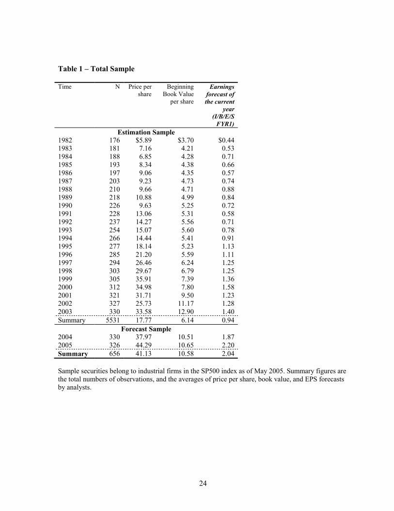
Table 1 shows the summary data in each included year. Year 1982 through Year 2003
constitute the estimation sample, which is the basis for identifying models and for forming estimation
parameters. Years 2004 and 2005 constitute the forecast sample. The estimation and forecast samples
are distinct from each other, and there is an increasing trend over time in all tabulated values.
<Table 1 about here>
Table 2 shows summary descriptive statistics for the estimation sample in Panel A, and the
forecast sample in Panel B. From Panel A for the estimation sample, the median values for price per
share and book per share are $15.06 and $4.08, respectively. The median FY1 forecast is $0.74, and
the median Treasury bill rate is 5.63%. From Panel B for the forecast sample, the median values for
price per share and book per share are $36.26 and $8.56, respectively. The median FY1 forecast is
$1.69, and the median quarterly Treasury bill rate is 1.89%. Values in the forecast sample are
generally larger than those in the estimation sample.
<Table 2 about here>
3.2. Diagnostics and Identification of Autocorrelation Models
To use Equation (9) in a regression analysis, the error term tv must meet the regression
assumptions. The first assumption is normality, which may matter severely if other assumptions are
not met. Further, the normal condition is important to infer that the structural form of the RIM

13
regression, which arises from ad-hoc truncation, is appropriate. I examine the statistical properties of
tv and report the results in Table 3. Figures 1 and 2 in Table 3 summarizes the distribution of tv ,
which shows near normality and a zero mean. Besides normality, I also examine stationarity because
lack of stationarity is a violation of constant variance, and stationarity is important for autocorrelation
modeling. Figure 3 is a time plot of tv , showing relative stationarity, albeit with some
heteroscedasticity (which will be addressed in Figure 6). Overall, tv seems satisfactory in terms of
normality and stationarity, suggesting that Equation (9) has an adequate structural form.
<Table 4 about here>
Another important assumption is that tv be independent and identically distributed random
variables (white noise), however this assumption is naïve. Because the estimation period includes
multiple years, I naturally expect strong serial correlation in all variables of Equation (9). Since the
seminal paper by Cochrane and Orcutt (1949), it is accepted econometric doctrine that serial
correlation in the regression error, or autocorrelation, leads to inefficient use of data, but much of this
inefficiency can be regained by transforming the error term to random. Many texts (for example
Greene 1990, Neter et al. 1990) describe the consequences of autocorrelation on estimation, namely
autocorrelation inflates the explanatory power of the estimation model, underestimates the estimated
parameters’ variances, and invalidates the models’ t and F tests. When the error term is not
independent, they contain information that can be used to improve the prediction of future values.
Theoretical guides to address autocorrelation are provided by Tsay (2002) and Shumway and Stoffer
(2006), and practical tutorials are provided in SAS Forecasting (1996).
Following Tsay (2002) and Shumway and Stoffer (2006), I use the autocorelation factors
(ACF) and the partial autocorrelation factors (PACF) to assess the time series properties of tv . These
factors can be produced by SAS Proc Arima. The ACF in Figure 4, which is cut off at lag 12 for
simpler exhibition, displays a nice exponential decay, consistent with an autoregressive positive
correlation. The PACF in Figure 5, which is also cut off at lag 12, shows a great spike after lag 1,

14
strongly indicating an AR(1) structure. The true underlying form is no doubt more complex, as the
PACF also shows smaller spikes at later lags, suggesting a higher order AR structure. Indeed, a
backstep procedure identifies autocorrelation through lag 5. Because there is a trade-off between
complexity and efficiency in modeling time series (Tsay 2002), I select the AR(1) and AR(2)
structures. Both encompass autocorrelation at lag 1, which accounts for most autocorrelation in the
data, while the AR(2) structure helps assess the merit of higher order AR structures.5
I also test for autocorrelation using generalized Durbin-Watson and Godfrey’s general
Lagrange Multiplier tests (Godfrey 1978a, 1978b). These tests can be produced with SAS Proc
Autoreg. From Figure 6, Durbin-Waston D is small, indicating strong positive correlation in the tv
series. Portmanteau Q is very large, indicating that tv is not white noise. Lagrange-Multiplier LM is
very large, indicating non-white noise and ARCH-type volatility. These statistics are consistent with
the findings in Figures 4-5, and further suggests volatility in the tv series. Volatility over time, also
termed conditional heteroscedasticity, is a special feature that Tsay (2002) addresses with GARCH
modeling. Following Tsay (2002, page 93), I select the basic GARCH model to assess volatility in
conjunction with the above-identified AR(2) structure. Table 4 describes all the regression models
identified from my data diagnostics.
<Table 4 about here>
It should be noted that, in Equation (9), the variables on the right-hand side correlate with
each other strongly. For example, in my estimation sample, book value per share and abnormal
earnings are significantly correlated with each other at p-value < 0.0001. This is not surprising, given
that book values and earnings are related accounting variables. Correlation among the right-hand-side
5 I eventually find that both work equally well, consistent with the wisdom that sophisticated time series models are not superior to the simple AR(1) model. In fact, the received empirical literature is overwhelmingly dominated by AR(1), as it is optimistic to expect to know precisely the correct form of autocorrelation in any situation (Greene 2000).
15
variables is often termed multi-collinearity, a situation which does not invalidate the models’ t and F
tests, and tends not to affect predictions of new observations (Neter et al. 1990).
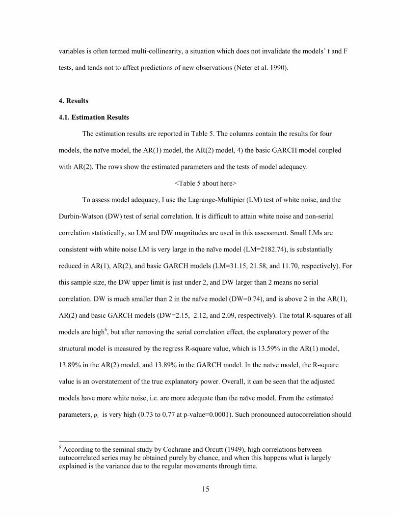
4. Results
4.1. Estimation Results
The estimation results are reported in Table 5. The columns contain the results for four
models, the naïve model, the AR(1) model, the AR(2) model, 4) the basic GARCH model coupled
with AR(2). The rows show the estimated parameters and the tests of model adequacy.
<Table 5 about here>
To assess model adequacy, I use the Lagrange-Multipier (LM) test of white noise, and the
Durbin-Watson (DW) test of serial correlation. It is difficult to attain white noise and non-serial
correlation statistically, so LM and DW magnitudes are used in this assessment. Small LMs are
consistent with white noise LM is very large in the naïve model (LM=2182.74), is substantially
reduced in AR(1), AR(2), and basic GARCH models (LM=31.15, 21.58, and 11.70, respectively). For
this sample size, the DW upper limit is just under 2, and DW larger than 2 means no serial
correlation. DW is much smaller than 2 in the naïve model (DW=0.74), and is above 2 in the AR(1),
AR(2) and basic GARCH models (DW=2.15, 2.12, and 2.09, respectively). The total R-squares of all
models are high6, but after removing the serial correlation effect, the explanatory power of the
structural model is measured by the regress R-square value, which is 13.59% in the AR(1) model,
13.89% in the AR(2) model, and 13.89% in the GARCH model. In the naïve model, the R-square
value is an overstatement of the true explanatory power. Overall, it can be seen that the adjusted
models have more white noise, i.e. are more adequate than the naïve model. From the estimated
parameters, ρ1 is very high (0.73 to 0.77 at p-value=0.0001). Such pronounced autocorrelation should
6 According to the seminal study by Cochrane and Orcutt (1949), high correlations between autocorrelated series may be obtained purely by chance, and when this happens what is largely explained is the variance due to the regular movements through time.
16
affect forecasts if not addressed. Book value per share and abnormal earnings are significantly
positive in all models, consistent with the theoretical RIM.
4.2. Forecast results
The forecasts are the corresponding regressions’ predicted outputs for one-year-ahead and
two-years-ahead beyond the estimation baseline. They are computed based on estimation results from
the estimation sample, which are applied to knowledge of beginning book values and FYR1 earnings
forecasts for the forecast years, and incorporated with the equivalent AR and GARCH parameters of
tv . Forecast can be produced by SAS Proc Autoreg, and are measured as follows.
Model 1 - Naïve:
.23,22
ˆˆˆˆˆ~
'
1~12101
=
=++=+
++
t
xxbvPt
a
ttt ββββ
Model 2 - AR(1):
.23,22
ˆ
ˆˆˆˆˆˆˆ~
'
1~12101
=
−=
+=+++=+
++
t
PP
xxbvP
ttt
tt
t
a
ttt
ν
νρβνρβββ
Model 3 - AR(2):
.23,22
ˆ
ˆ
ˆˆˆˆˆˆˆˆˆ
111
121~
'
1~12112101
=
−=
−=
++=++++=
−−−
−+
−++
t
PP
PP
xxbvP
ttt
ttt
ttt
tt
a
ttt
ν
ν
νρνρβνρνρβββ
Model 4 - AR(2) Basic GARCH:

17
.23,22
1;0,0,0);1,0(~
ˆ
ˆ
ˆˆˆˆˆˆˆˆˆˆˆ
111101
2
1
2
10
2
1
111
111
1121~
'
1~112112101
=
<+≥≥>
++=
=
−=
−=
+++=+++++=
+
+
+++
−−−
+−+
+−++
t
Ne
hh
eh
PP
PP
xxbvP
t
ttt
ttt
ttt
ttt
tttt
ttt
a
ttt
γαγαα
γεαα
ε
ν
ν
ενρνρβενρνρβββ
Empirically, it remains to be seen if the adjusted models are indeed better at predicting future
stock prices. In the following, the forecast performance of each model is assessed based on three
measurements, mean error (ME), mean absolute percentage error (MAPE), and mean squared
percentage error (MSPE). ME, the difference between forecast and actual prices scaled by actual
price, is a measure of forecast bias as it indicates whether forecast values are systematically lower or
higher than actual values. MAPE, the absolute difference between forecast and actual prices scaled by
actual price, is a measure of forecast accuracy. MSPE, the square of ME, is a measure of forecast
accuracy that can accentuate large errors. Steps-ahead forecasts are predictions from the respective
regressions for new observations.
Panel A of Table 6 shows the forecast results for 2004 (one-year-ahead). As presented, all
models have average negative MEs, indicating that model forecasts are smaller than actual price.
Understandably, the naïve model performs the worst, having the most negative ME (mean = -8.91%,
median = -16.60%. The AR(1) model has a mean ME of -6.62%, slightly better than the GARCH
model (with mean ME = -6.70%) and the AR(2) model (with mean ME = -6.88%).
<Table 6 about here>
As to the results of MAPE, the naïve model stands out as the worst, having the largest MAPE
(mean = 29.33%, median = 24.59%). The GARCH model has the smallest MAPE (mean = 18.12%
and median = 14.93%). The AR(1) and AR(2) models have slightly larger MAPE (with mean =
19.47% and 19.41%, respectively). Similarly, from the results of MSPE, the naïve model performs
18
the worst, having the largest MSPE (mean = 15.05%, median = 6.05%), whereas MSPE is 7.12%,
7.00%, and 5.27% in the AR(1), AR(2), and GARCH models, respectively.
Panel B of Table 6 presents the forecast results for 2005 (two-years-ahead). The naïve model
yields the worst errors, with MAPE, MSPE and ME equal to 49.24%, 883.78%, and -24.78%. The
GARCH model produces the best accuracy, producing the smallest MAPE (mean= 29.42%) and
MSPE (mean=28.57%), and the smallest magnitude of ME (mean=-0.06%). The AR(1) model is the
next best, with mean MAPE, MSPE and ME equal to 32.77%, 74.25%, and -11.58%, respectively.
The AR(2) model is very comparable to the AR(1) model, with MAPE, MSPE and ME equal to
32.95%, 83.42%, and -12.02%, respectively.
It is appropriate to conclude from the results that, because all models in Tables 7 and 8 are
implemented using the same data and estimation procedures except for the adjustment of
autocorrelation, this adjustment reduces forecast errors.
To assess the ability of time series models of tv , one can compare the AR(1) and AR(2)
models. Theoretically the AR(2) model should be better because it accounts for autocorrelation more
completely than the AR(1) model. However, the empirical results do not show marked advantage of
one over the other. This underlines the trade-off between completeness and efficiency: while AR(2) is
a more complete model, it requires more data and is more complex to apply than AR(1). On the other
hand, the GARCH model, which addresses both auto correlation and volatility, performs better than
the others. Overall, Section 4 shows that adjusting for autocorrelation leads to more adequate
estimation models and more accurate prediction models. Better estimation models help better explain
contemporaneous stock prices, while better prediction models improve forecasts of future stock
prices.
5. Extension Analyses to Address Scale Effects
A concern is that scale differences may affect regression results. Scale differences arise
because large (small) firms have large (small) values of many variables. Cross-sectionally, scale

19
differences exist when large and small firms are sampled together (Barth and Kallapur 1996).
Serially, scale differences arise when firms have inconsistent scale over time, for example due to
stock splits and stock dividends (Brown et al. 1999). Barth and Kallapur (1996) discuss that scale
differences result in heteroscedastic regression error variances, which lead to coefficient bias if the
magnitude differences are unrelated to the research question. According to Brown et al. (1999), a
scale-affected regression will have higher R-square than that from the same regression without scale
effects. Many studies discuss the scale problem and seek to address it (for example, Lo and Lys 2000,
Barth and Kallapur 1996, Kothari and Zimmerman 1995, and Sougiannis 1994). Some common
accounting scale proxies are total assets, sales, book value of equity, net income, number of shares,
and share price, and many authors deflate by a scale proxy to address scale differences (Barth and
Kallapur 1996). For example, Kothari and Zimmerman (1995) scale by number of shares, and
Sougiannis (1994) by total assets.
My reported results should not be affected severely by scale differences because I use large
SP500 firms only, I deflate by number of shares, which is one common method to address cross-
sectional scale differences, and I adjust shares for splits, stock dividends and other capital
adjustments. However, because scale concern is pervasive, I replicate the analyses using two
additional scaling schemes, namely scaling by beginning total assets, and using no scale. I adjust the
three differently-scaled models for autocorrelation and produce price forecasts. In each of the three
models, I aim to show that forecasts after adjusting for autocorrelation are more accurate than those
formed naively (i.e., before adjusting for autocorrelation).
Panel A of Table 7 presents the diagnostics of the naïve model from Table 4, which is scaled
by number of shares. Panels B and C present the diagnostics of the same model, but no deflation is
used in Panel B, and all RIM variables are deflated by beginning total assets instead of number of
shares in Panel C. To ensure a good comparison, all three models are based on precisely the same
sample and procedures except for the deflation factor. From the data already collected, 5,353
observations that have beginning total assets are used in the scale analyses reported in Tables 8 and 9.

20
<Table 7 about here>
Table 7 shows the diagnostics of tv in three differently-scaled models. The share-deflated
distribution is the closest to normality compared to the other distributions which are highly skewed
and highly peaked. All three models suffer from heteroscedasticity and autocorrelation. All three
could benefit from techniques to address heteroscedasticity, however, the share-deflated model has
the least amount of error variability. All three models have significant autocorrelation, however the
asset-deflated model has the least autocorrelation relative to the others. In sum, all models have
different types of violations to different extents.
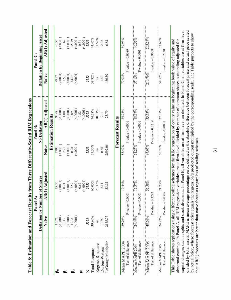
Table 8 shows the estimation and forecast results from the three models. The naïve and
AR(1) adjusted results are reported for each of the models. Because of different scales, R-square
values cannot be used for comparison. All three adjusted models are deemed adequate judging from
their levels of white noise (low LaGrange Multiplier and Durbin-Watson above 2). However, from
the forecast results, the share-deflated model yields the lowest forecast errors, and the asset-deflated
model yields the worst forecasts. Tables 8 and 9 yield insight consistent with Rawlings et al. (2001):
for forecasting purpose, non-normality may affect forecasts severely, although its effect on estimation
is not apparent.
<Table 8 about here>
The forecast results of Table 8 show lower adjusted MAPEs than naïve MAPEs for each of
the three differently-scaled models. For example, in the un-deflated model, the median naïve MAPE
is 51.27%, contrasted to the adjusted median of 18.67%, for a difference significant at p-value
<.0001. In fact, for all three models, the difference between naïve and adjusted MAPEs is statistically
different in both mean and median tests for 2004 forecasts. For 2005 forecasts, all tests of difference
are significant except the mean test from the share-deflated model and the tests from the asset-
deflated model. Overall, adjusted MAPEs are statistically lower than naïve MAPEs in all scaling
schemes, supporting the conclusion that adjusting for autocorrelation improves price forecasts.

21
6. Summary and Conclusion
For the purpose of equity valuation, it is important to assess the true fundamental economic
strengths of a firm. Over the past decade, the Residual Income Model (RIM) has become widely
accepted as a theoretical framework for equity valuation based on fundamental information from
accounting data. Successful applications of the RIM are desirable to contribute a fundamental
perspective to pricing decisions.
Measuring abnormal earnings as the difference between analyst forecast and the cost of
capital charge, this paper demonstrates a method to forecast stock price by applying the RIM, with
adjustment for autocorrelation. A regression to adapt the theoretical RIM for cross-sectional empirical
analyses models stock price as a function of book value at the beginning of the year, abnormal
earnings of the current year defined as earnings forecasts of the current year minus a normal capital
charge, and an unknown term tv . After introducing the RIM, this paper shows how to implement the
basic RIM with one term of abnormal earnings, and how to address autocorrelation in the RIM
regression to improve forecast accuracy. The method to address autocorrelation is by diagnosing tv to
identify its proper structures, and then model the RIM regression jointly with the identified structures
of tv . Based on a concrete example of SP500 firms, the approach demonstrated in this paper results
in a mean absolute percentage error as low as 18.12% in one-year-ahead forecasts and 29.42% in two-
year-ahead forecasts.
Overall, this paper complements other valuation methods by blending fundamental
accounting data and mechanical analyses of trends. It is noted that due to other econometric problems
than autocorrelation in large and heterogeneous samples, the usefulness of adjusting for
autocorrelation is best demonstrated with large firms.

22
References:
BARTH, M., AND KALLAPUR, S. “The Effects of Cross-Sectional Scale Differences on Regression Results in Empirical Accounting Research.” Contemporary Accounting Research 13 (Fall 1996): 527-567.
BROWN, S.; K. LO; AND T. LYS. “Use of R-square in Accounting Research: Measuring Changes in Value Relevance over the Last Four Decades” Journal of Accounting Research (December 1999): 83-115.
CALLEN, J. L., AND M. MOREL. “Linear Accounting Valuation When Abnormal Earnings are AR
(2)” Review of Quantitative Finance & Accounting (May 2001): 191-203. CHOI, Y.; J. E. O’HANLON; AND P. POPE. “Comparative Accounting and Linear Information
Valuation Models” Contemporary Accounting Research 23 (Spring 2006): 73-101. COCHRANE, D., AND G.H. ORCUTT. “Application of Least Squares Regression to Relationships
Containing Auto-Correlated Error Terms” Journal of the American Statistical Association 44
(March 1949): 32-61.
COURTEAU, L.; J. KAO; AND G.D. RICHARDSON. “Equity Valuation Employing the Ideal versus Ad Hoc Terminal Value Expressions” Contemporary Accounting Research 18 (Winter 2001): 625-661.
DECHOW, P. M., AND A. P. HUTTON. “An Empirical Assessment of the Residual Income Valuation Model” Journal of Accounting & Economics (January 1999): 1-34.
FRANCIS, J.; P. OLSSON; AND R. DENNIS. “Comparing the Accuracy and Explainability of
dividend, Free Cash Flow, and Abnormal Earnings Equity Value Estimates” Journal of
Accounting Research (Spring 2000): 45-70. FRANKEL, R., AND C. M. C. LEE. “Accounting Valuation, Market Expectation, and Cross-
sectional Stock Returns” Journal of Accounting and Economics (June 1998): 283-319. GREENE, W. H. Econometric Analysis. Fourth Edition. Prentice Hall. 2000. GODFREY, L. “Testing against General Autoregressive and Moving Average Error Models When
the Regressors Include Lagged Dependent Variables” Econometrica 46 (1978a): 1293-1301. GODFREY, L. “Testing against General Autoregressive and Moving Average Error Models When
the Regressors Include Lagged Dependent Variables” Econometrica 46 (November 1978a): 1293-1301.
GODFREY, L. “Testing for Higher Order Serial Correlation in Regression Equations When the
Regressors Include Lagged Dependent Variables” Econometrica 46 (November 1978b): 1303-1310.
HAND, J. “Discussion of Earnings, Book Values, and Dividends in Equity Valuation: An Empirical
Perspective” Contemporary Accounting Research (Spring 2001): 212-130.

23
KOTHARI, S. P., AND ZIMMERMAN, J. L. Journal of Accounting & Economics, (September 1995): 155-192.
LO, K., AND T. LYS. “The Ohlson Model: Contribution to Valuation Theory, Limitations, and
Empirical Applications”, Journal of Accounting, Auditing, and Finance 15 (Summer 2000): 337-367.
LUNDHOLM, R. J., AND T. B. O’KEEFE. “On Comparing Cash Flow and Accrual Accounting
Models for the Use in Equity Valuation: A Response to Penman” Contemporary Accounting
Research (Winter 2001): 681-696. MYERS, J. N. “Implementing Residual Income Valuation with Linear Information Dynamics”
Accounting Review (January 1999): 1-28. NETER, J.; W. WASSERMAN; AND M. KUTNER. Applied Linear Statistical Models – Regression,
Analysis of Variance, and Experimental Designs. Irwin (1990).
OHLSON, J. A. “Earnings, Book Values, and Dividends in Equity Valuation” Contemporary
Accounting Research (Spring 1995): 661-687. PEASNELL, K. V. “Some Formal Connections Between Economic Values and Yields and
Accounting Numbers”, Journal of Business Finance & Accounting (Autumn 1982): 361-381. PENMAN, S. H., AND T. SOUGIANNIS. “A Comparison of Dividend, Cash Flow, and Earnings
Approaches to Equity Valuation”, Contemporary Accounting Research (Autumn 1998): 45-70.
RAWLINGS, J.O. Applied Regression Analysis: A Research Tool. Springer. 2001. RUBINSTEIN, M. “The Valuation of Uncertain Income Streams and the Pricing of Options” Bell
Journal of Economics (Autumn 1976): 407-408. SAS PUBLISHING. “Forecasting Examples For Business and Economics Using SAS”. 1996. SAS
Institute Inc., Cary NC, USA. SHUMWAY, R. H., AND D. STOFFER. Time Series Analysis and Its Applications. Springer. May
2006. SOUGIANNIS, T. ‘The Accuracy and Bias of Equity Values Inferred from Analysts’ Earnings
Forecasts” Journal of Accounting, Auditing, and Finance (January 1994): 331-362. SOUGIANNIS, T., AND T. YAEKURA. “The Accuracy and Bias of Equity Values Inferred from Analysts’ Earnings Forecasts” Journal of Accounting, Auditing, and Finance (Fall 2001): 331-362 TSAY, R. S. Analysis of Financial Time Series. John Wiley & Sons. 2002.
24
Table 1 – Total Sample
Time N Price per
share Beginning Book Value per share
Earnings
forecast of
the current
year
(I/B/E/S
FYR1)
Estimation Sample
1982 176 $5.89 $3.70 $0.44 1983 181 7.16 4.21 0.53 1984 188 6.85 4.28 0.71 1985 193 8.34 4.38 0.66 1986 197 9.06 4.35 0.57 1987 203 9.23 4.73 0.74 1988 210 9.66 4.71 0.88 1989 218 10.88 4.99 0.84 1990 226 9.63 5.25 0.72 1991 228 13.06 5.31 0.58 1992 237 14.27 5.56 0.71 1993 254 15.07 5.60 0.78 1994 266 14.44 5.41 0.91 1995 277 18.14 5.23 1.13 1996 285 21.20 5.59 1.11 1997 294 26.46 6.24 1.25 1998 303 29.67 6.79 1.25 1999 305 35.91 7.39 1.36 2000 312 34.98 7.80 1.58 2001 321 31.71 9.50 1.23 2002 327 25.73 11.17 1.28 2003 330 33.58 12.90 1.40
Summary 5531 17.77 6.14 0.94
Forecast Sample
2004 330 37.97 10.51 1.87 2005 326 44.29 10.65 2.20
Summary 656 41.13 10.58 2.04
Sample securities belong to industrial firms in the SP500 index as of May 2005. Summary figures are the total numbers of observations, and the averages of price per share, book value, and EPS forecasts by analysts.

25
Table 2: Descriptive Statistics
Panel A: Estimation Sample (5531 firm-years in 1982 – 2003)
Min 5% 25% Median 75% 95% Max Mean
Price per share (N=5531) 0.07 1.77 6.90 15.06 28.24 52.14 126.98 19.68 Beginning Book Value per Share (N=5531) 0.00 0.31 1.68 4.08 8.23 19.14 703.34 6.53
EPS forecast of the current year (N=5531) -5.83 0.02 0.31 0.74 1.44 2.93 8.51 1.00
Annual treasury bill rate (N=22) 1.24 1.24 3.89 5.63 7.65 10.91 12.27 5.79
Panel B: Forecast Sample (656 firm-years in 2004 – 2005)
Min 5% 25% Median 75% 95% Max Mean
Price per share 0.29 10.18 24.46 36.26 51.26 74.40 107.96 38.69 Beginning Book Value per Share (N=656) 0.00 2.00 5.27 8.56 13.33 23.16 345.89 10.58
EPS forecast of the current year (N=656) -4.11 0.14 1.02 1.69 2.69 5.12 10.81 2.04
Annual treasury bill rate (N=2) 1.89 1.89 1.89 1.89 3.62 3.62 3.62 2.75
All values are reported in US dollars, except Treasury bill rate which is in %. All firm data are adjusted for capital changes, including stock splits and stock dividends. Book value is computed as total assets minus total liabilities minus preferred stocks, divided by common shares outstanding. EPS forecasts of the current year is I/B/E/S FYR1 forecasts. Annual treasury bill rate is market yield on U.S. Treasury securities at 1-year constant maturity, quoted on investment basis, as released by the Federal Reserve.

Table
3: D
iagnost
ics of
tv
N= 5531
Mean = 0
Median = -3.61
Range = 688.53
Interquartile range = 12.52
Standard Deviation = 12.85
Skewness = 1.53
Kurtosis = 7.84
Figure 1
Distribution
hhiggins 26FEB07
-124
-108
-92
-76
-60
-44
-28
-12
420
36
52
68
84
100
05
10
15
20
25
30
35
40
P e r c e n t
r
Figure 2
Histogram
hhiggins 26FEB07
r
-200
-1000
100
Time
010
20
30
Figure 3
Time Plot
Lag -1 9 8 7 6 5 4 3 2 1 0 1 2 3 4 5 6 7 8 9 1
1 | |********************|
2 | .|************ |
3 | .|******** |
4 | .|***** |
5 | .|*** |
6 | .|** |
7 | .|* |
8 | .| |
9 | *| |
10 | *| |
11 | .*|. |
12 | .*|. |
Figure 4
Autocorrelations (ACF)
Lag -1 9 8 7 6 5 4 3 2 1 0 1 2 3 4 5 6 7 8 9 1
1 | .|************ |
2 | |. |
3 | |. |
4 | |. |
5 | *| |
6 | |. |
7 | *|. |
8 | .|. |
9 | *|. |
10 | .|. |
11 | *|. |
12 | .|. |
Figure 5
Partial Autocorrelations (PACF)
Durbin-Watson D = 0.7353
Pr> D: <0.0001
Portmanteau Q= 3269.17
Pr>Q: < 0.0001
Lagrange Multiplier = 1875.35
Pr>LM: <0.0001 Figure 6
Autocorrelation and ARCH disturbances
The diagnostics of
tvare to assess the appropriateness of the naive RIM regression
,where
tv is the error term,
tP is stock price per share at time,
1−t
bv
is book value per share at the beginning of the current annual period which
starts at t-1 and ending at t,
a tx is abnormal earnings over the current period, defined as
1−
−=
tt
t
a tbv
rx
x,
txis EPS forecast over the current
period (I/B/E/S FYR1 earnings forecast), and
tr is the current Treasury bill rate. The distribution in Figure 1 and histogram in Figure 2 show near
normality. The time plot in Figure 3 shows stationarity and some heteroscedasticity. Autocorrelation factors in Figures 4 and 5 show
autoregressive pattern. Generalized Durbin-Watson tests and Godfrey’s general Lagrange Multiplier test in Figure 6 show dependence, non-white
noise, and ARCH disturbances.
t
a tt
tv
xbv
P+
++
=−
21
10
ββ
β

27
Table
4: R
IM R
egres
sions
Model
Equation
1
Naïve
2
AR(1)
3
AR(2)
4
AR(2)
Basic GARCH
Table 4 shows the models identified from the diagnostics in Table 3.
tP is stock price per share at time t,
1−t
bv
is book value per share at the
beginning of the current annual period which starts at t-1 and ending at t,
a tx is abnormal earnings over the current period which I define as
1−
−=
tt
t
a tbv
rx
x,
txis EPS forecast over the current period (I/B/E/S FYR1 earnings forecast),
tr is the current Treasury bill rate,
tv is the error
term,
tεis the disturbance term,
20−
β are RIM regression parameters,
21−ρ
are autocorrelation parameters, and
10−
α and 1γ are GARCH
parameters. The naïve model does not address autocorrelation. The AR(1) and AR(2) models assume
tv follows an AR(1) and an AR(2) structure,
respectively. The AR(2) - GARCH model combines AR(2) assumption and GARCH modeling of
tv.
),0(
~,
,2
21
10
σε
εβ
ββ
Nv
vx
bv
Pii
d
tt
tt
a tt
t=
++
+=
−
),0(
~,
,2
12
11
0σ
εε
ρβ
ββ
Nv
vv
xbv
Pii
d
tt
tt
t
a tt
t+
=+
++
=−
−
),0(
~,
,2
22
11
21
10
σε
ερ
ρβ
ββ
Nv
vv
vx
bv
Piid
tt
tt
tt
a tt
t+
+=
++
+=
−−
−
1;0
,0
,0
);1,0(
~,
,,
,
11
11
0
2
11
2
11
0
2
22
11
21
10
<+
≥≥
>+
+=
=+
+=
++
+=
−−
−−
−
γα
γα
αγ
εα
α
εε
ρρ
ββ
β
Ne
hh
eh
vv
vv
xbv
P
tt
tt
tt
tt
tt
tt
a tt
t

Table 5: Estimation Results of RIM Regressions
Estimated Coefficients
(p-value) and
Model Statistics
Naïve AR(1) AR(2) AR(2)
GARCH
ββββ0 0 0 0 Intercept 10.51 (<.0001)
14.96 (<.0001)
14.92 (<.0001)
28.81 (<.0001)
ββββ1111 Book Value 0.34 (<.0001)
0.17 (<.0001)
0.17 (<.0001)
0.05 (<.0001)
ββββ2 2 2 2 Abnormal Earnings
10.38 (<.0001)
5.54 (<.0001)
5.60 (<.0001)
3.20 (<.0001)
ρρρρ1 1 1 1 AR Parameter
0.75 (<.0001)
0.73 (<.0001)
0.77 (<.0001)
ρρρρ2 2 2 2 AR parameter
-0.02 (=.1771)
0.17 (<.0001)
αααα0000 GARCH parameter
0.28 (<.0001)
αααα1 1 1 1 GARCH parameter
0.01 (<.0001)
γγγγ1 1 1 1 GARCH parameter
0.01 (<.0001)
N 5531 5531 5531 5531
Total R-square 40.45% 70.69% 70.67% 75.55%
Regress R-square n/a 13.59% 13.89% 13.89%
Durbin-Watson 0.74 2.15 2.12 2.09
LaGrange Multiplier 2182.74 31.15 21.58 11.70
The regression models have the same structural form but different treatments for autocorrelation. The structural form is
where tP is stock price per share at time, 1−tbv is book value per share at the beginning of the
current annual period which starts at t-1 and ending at t, a
tx is abnormal earnings over the current
period which I define as 1−−= ttt
a
t bvrxx , tx is EPS forecast over the current period (I/B/E/S
FYR1 earnings forecast), tr is the current Treasury bill rate, and tv is the error term. 20−β are
RIM regression parameters, 21−ρ are autocorrelation parameters, and 10−α and 1γ are GARCH
parameters. The naïve model does not address autocorrelation. The AR(1) and AR(2) models
assume tv follows an AR(1) and an AR(2) structure, respectively. The AR(2) - GARCH model
combines AR(2) assumption and GARCH modeling of tv . Each model is assessed for
explanatory power using regress R-square, autocorrelation using Durbin-Watson generalized test, and white noise using LaGrange Multiplier test.
t
a
ttt vxbvP +++= − 2110 βββ

29
Table 6: Forecast Results
Panel A: 2004 (N=330) – One-Year-Ahead
Mean
[Median]
Naïve AR(1) AR(2) AR(2)
GARCH
ME
-8.91% [-16.60%]
-6.62% [-10.77%]
-6.88% [-10.72%]
-6.70% [-10.73%]
MAPE
29.33% [24.59%]
19.47% [16.46%]
19.41% [15.58%]
18.12% [14.93%]
MSPE
15.05% [6.05%]
7.12% [2.39%]
7.00% [2.43%]
5.27% [2.23%]
Panel B: 2005 (N=326) – Two-Years-Ahead
Mean
[Median]
Naïve AR(1) AR(2) AR(2)
GARCH
ME
-24.78% [-16.53%]
-11.58% [-14.94%]
-12.02% [-14.51%]
-0.06% [-10.92%]
MAPE
49.24% [25.07%]
32.77% [21.42%]
32.95% [21.49%]
29.42% [20.19%]
MSPE
883.78% [6.29%]
74.25% [4.59%]
83.42% [4.62%]
28.57% [4.08%]
Stock price forecasts are predicted values from RIM regressions sharing the same structural form but differing in the treatments for autocorrelation. The structural form is
: where tP is stock price per share at time, 1−tbv is book value per share at the beginning of the
current annual period which starts at t-1 and ending at t, a
tx is abnormal earnings over the current
period defined as 1−−= ttt
a
t bvrxx , tx is EPS forecast over the current period (I/B/E/S FYR1
earnings forecast), tr is the current Treasury bill rate, and tv is the error term.
The naïve model does not address auto correlation. The AR(1) and AR(2) models assume
tv follows an AR(1) and an AR(2) structure, respectively. The AR(2) - GARCH model combines
AR(2) and GARCH modeling of tv .
The forecasts are the corresponding regressions’ predicted outputs for one-year-ahead and two-years-ahead beyond the estimation baseline. They are computed based on estimation results from the estimation sample, which are applied to knowledge of beginning book values and FYR1 earnings forecasts for the forecast years, and incorporated with the equivalent AR and GARCH
parameters of tv .
The forecast results are assessed based on three forecast error measures. MAPE is mean average percentage error, defined as the absolute difference between forecast price and actual price scaled by actual price. ME is the mean error, defined as the signed difference between forecast price and actual price scaled by actual price. MSE is the mean squared error, defined as the squared difference between forecast price and actual price scaled by the squared actual price.
t
a
ttt vxbvP +++= − 2110 βββ

Table
7: D
iagnost
ics of th
e Err
or
Ter
m fro
m T
hre
e D
iffe
rently-S
cale
d R
IM R
egres
sions
Panel
A: D
efla
tion b
y N
um
ber
of Share
s Panel
B: N
o D
efla
tion
Panel
C: D
efla
tion b
y B
egin
nin
g A
sset
hhiggins 09MAR07
-120
-104
-88
-72
-56
-40
-24
-8
824
40
56
72
88
0
10
20
30
40
50
P e r c e n t
r
hhiggins 09MAR07
-400000
-280000
-160000
-40000
80000
200000
320000
440000
560000
05
10
15
20
25
30
35
40
45
50
55
60
65
70
75
80
85
90
95
100
P e r c e n t
Rr
hhiggins 09MAR07
-24
-8
824
40
56
72
88
104
120
136
152
168
184
200
0
20
40
60
80
100
P e r c e n t
Sr
N= 5353
Mean = 0
Median = -3.57
Range = 216.05
Interquartile range = 12.80
Standard Deviation = 12.94
Prob > White's Chi-square < 0.0001
Variability = -3.62
Skewness = 1.53
Kurtosis = 7.51
Durbin-Watson D = 0.75
(Pr < D: <0.0001 Positive correlation)
N= 5353
Mean = 0
Median = -3,535.12
Range = 954,383
Interquartile range = 3,687
Standard Deviation = 24,862
Prob > White's Chi-square < 0.0001
Variability = -7.03
Skewness = 6.36
Kurtosis = 120.16
Durbin-Watson D = 0.66
(Pr<D: <0.0001 Positive correlation)
N= 5353
Mean = 0
Median = -0.37
Range = 223.16
Interquartile range = 1.50
Standard Deviation = 5.44
Prob > White's Chi-square = 0.0087
Variability = -14.70
Skewness = 21.68
Kurtosis = 662.12
Durbin-Watson D = 1.40
(Pr<D: <0.0001 Positive correlation)
This Table shows replications using different scaling schemes for the RIM regression of equity value on beginning book value of equity and
abnormal earnings. In Panel A, all regression variables are at firm-level divided by number of common shares outstanding adjusted for capital
adjustments including stock splits and dividends. In Panel B, all variables are at firm level un-deflated. In Panel C, all variables are at firm-level
divided by total assets. The diagnostics assess the distribution and autocorrelation properties of the error terms.
31
Table
8: E
stim
ation a
nd F
ore
cast
Res
ults fr
om
Thre
e D
iffe
rently-S
cale
d R
IM R
egre
ssio
ns
Panel
A:
Def
lation b
y N
um
ber
of Share
s
Panel
B:
No D
efla
tion
Panel
C:
Def
lation b
y B
egin
nin
g A
sset
Naïv
e A
R(1
) A
dju
sted
N
aïv
e A
R(1
) A
dju
sted
N
aiv
e A
R(1
) A
dju
sted
E
stim
ation R
esults
β βββ0 000
10.76
(<.0001)
13.50
(<.0001)
3703
(<.0001)
9198
(<.0001)
-0.57
(<.0001)
-0.57
(<.0001)
β βββ1 111
0.33
(<.0001)
0.21
(<.0001)
2.91
(<.0001)
1.00
(<.0001)
1.50
(<.0001)
1.46
(<.0001)
β βββ2 222
10.36
(<.0001)
7.59
(<.0001)
0.28
(<.0001)
0.09
(<.0001)
34.96
(<.0001)
35.19
(<.0001)
ρ ρρρ1 111
0.67
(<.0001)
0.82
(<.0001)
0.31
(<.0001)
N
5353
5353
5353
5353
5353
5353
Total R-square
39.96%
65.03%
37.30%
74.38%
38.92%
44.47%
Regress R-square
na
23.37%
na
10.03%
na
31.57%
Durbin-Watson
0.75
2.11
0.66
2.11
1.40
2.02
LaGrange Multiplier
2135.77
33.92
2592.06
25.79
486.50
6.82
Forec
ast
Res
ults
Mean MAPE 2004
29.76%
19.44%
83.47%
24.73%
77.93%
59.93%
Test of difference
P-value <0.0001
P-value <0.0001
P-value = 0.0089
Median MAPE 2004
24.49%
15.37%
51.27%
18.67%
57.15%
40.55%
Test of difference
P-value <0.0001
P-value <0.0001
P-value <0.0001
Mean MAPE 2005
48.76%
32.58%
97.07%
53.73%
210.76%
203.24%
Test of difference
P-value = 0.3293
P-value = 0.0219
P-value = 0.9608
Median MAPE 2005
24.72%
21.23%
50.77%
27.07%
58.52%
52.67%
Test of difference
P-value = 0.0307
P-value <0.0001
P-value = 0.2730
This Table shows replications using different scaling schemes for the RIM regression of equity value on beginning book value of equity and
abnormal earnings. In Panel A, all RIM regression variables are at firm-level divided by number of common shares outstanding adjusted for
capital changes such as splits and stock dividends. In Panel B, all variables are at firm level un-deflated. In Panel C, all variables are at firm-level
divided by total assets. MAPE is mean average percentage error, defined as the absolute difference between forecast price and actual price scaled
by actual price, where forecast price equals the regression’s predicted output multiplied by the corresponding scale. The Table purports to show
that AR(1) forecasts are better than naïve forecasts regardless of scaling schemes.
